Training Invertible Linear Layers through Rank-One Perturbations

Abstract

Many types of neural network layers rely on matrix properties such as invertibility or orthogonality. Retaining such properties during optimization with gradient-based stochastic optimizers is a challenging task, which is usually addressed by either reparameterization of the affected parameters or by directly optimizing on the manifold. This work presents a novel approach for training invertible linear layers. In lieu of directly optimizing the network parameters, we train rank-one perturbations and add them to the actual weight matrices infrequently. This P⁴Inv update allows keeping track of inverses and determinants without ever explicitly computing them. We show how such invertible blocks improve the mixing and thus the mode separation of the resulting normalizing flows. Furthermore, we outline how the P⁴ concept can be utilized to retain properties other than invertibility.

1 Introduction

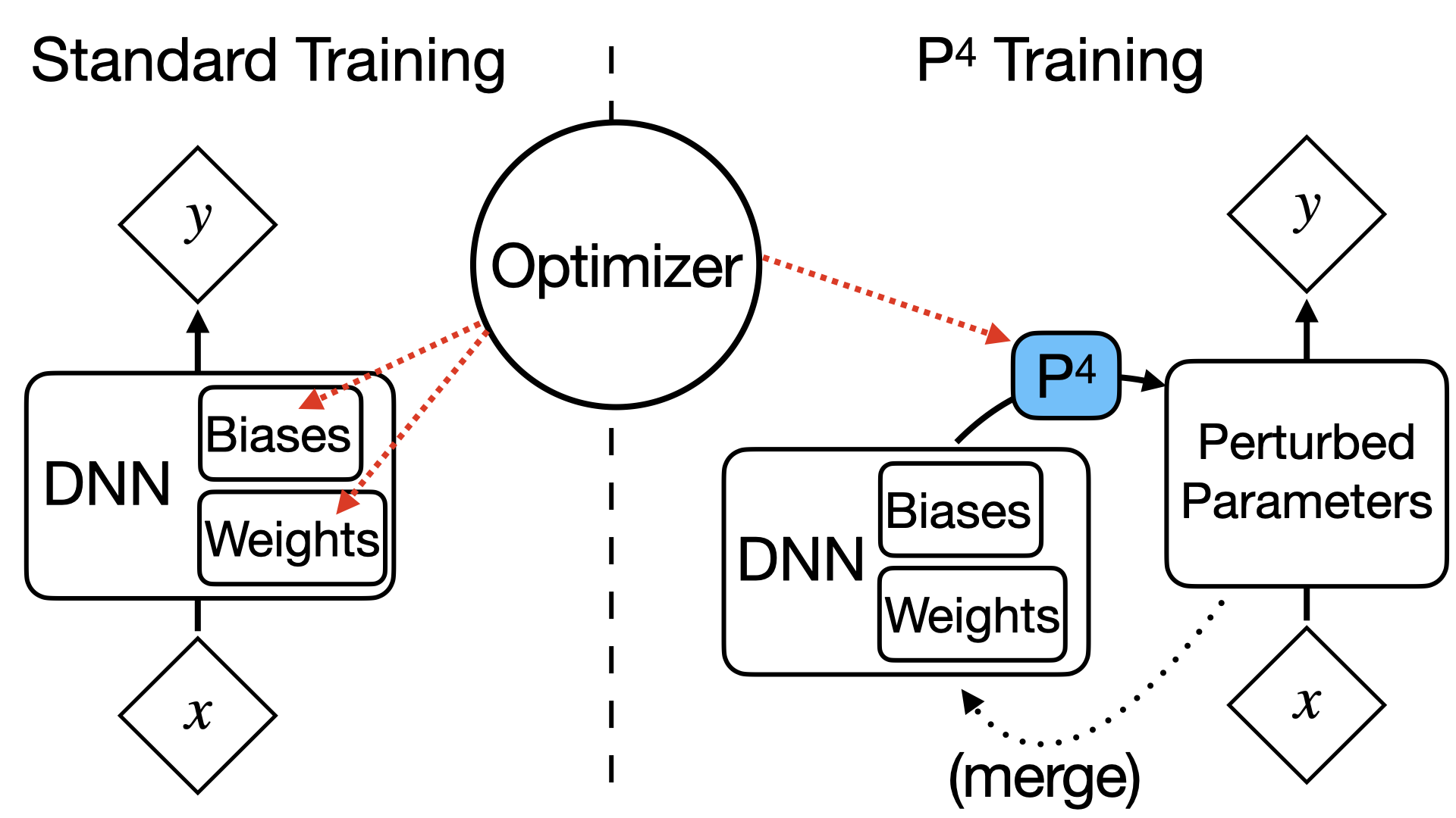
Figure 1: Training of deep neural networks (DNN). Standard DNN transform inputs $x$ into outputs $y$ through activation functions and linear layers, which are tuned by an optimizer. In contrast, P⁴ training operates on perturbations to the parameters. Those are defined to retain certain network properties (here: invertibility as well as tractable inversion and determinant computation). The perturbed parameters are merged in regular intervals.

Many deep learning applications depend critically on the neural network parameters having a certain mathematical structure. As an important example, reversible generative models rely on invertibility and, in the case of normalizing flows, efficient inversion and computation of the Jacobian determinant (Papamakarios et al., 2019).

Preserving parameter properties during training can be challenging and many approaches are currently in use. The most basic way of incorporating constraints is by network design. Many examples could be listed, like defining convolutional layers to obtain equivariances, constraining network outputs to certain intervals through bounded activation functions, Householder flows (Tomczak & Welling, 2016) to enforce layer-wise orthogonality, or coupling layers (Dinh et al., 2014; 2016) that enforce tractable inversion through their two-channel structure. A second approach concerns the optimizers used for training. Optimization routines have been tailored for example to maintain Lipschitz bounds (Yoshida & Miyato, 2017) or efficiently optimize orthogonal linear layers (Choromanski et al., 2020).

The present work introduces a novel algorithmic concept for training invertible linear layers and facilitate tractable inversion and determinant computation, see Figure 1. In lieu of directly changing the network parameters, the optimizer operates on perturbations to these parameters. The actual network parameters are frozen, while a parameterized perturbation (a rank-one update to the frozen parameters) serves as a proxy for optimization. Inputs are passed through the perturbed network during training. In regular intervals, the perturbed parameters are merged into the actual network and the perturbation is reset to the identity. This stepwise optimization approach will be referred to as property-preserving parameter perturbation, or P⁴ update. A similar concept was introduced recently by Lezcano-Casado (2019), who used dynamic trivializations for optimization on manifolds.

In this work, we use P⁴ training to optimize invertible linear layers while keeping track of their inverses and determinants using rank-one updates. Previous work (see Section 2) has mostly focused on optimizing orthogonal matrices, which can be trivially inverted and have unity determinant. Only most recently, Gresele et al. (2020) presented a first method to optimize general invertible matrices implicitly using relative gradients, thereby providing greater flexibility and expressivity. While their scheme implicitly tracks the weight matrices’ determinants, it does not facilitate cheap inversion. In contrast, the present P⁴Inv layers are inverted at the cost of roughly three matrix-vector multiplications.

P⁴Inv layers can approximate arbitrary invertible matrices ${\bm{A}}\in\mathrm{GL}(n)$. Interestingly, our stepwise perturbation even allows sign changes in the determinants and recovers the correct inverse after emerging from the ill-conditioned regime. Furthermore, it avoids any explicit computations of inverses or determinants. All operations occurring in optimization steps have complexity of at most $\mathcal{O}(n^{2}).$ To our knowledge, the present method is the first to feature these desirable properties.

We show how P⁴Inv blocks can be utilized in normalizing flows by combining them with nonlinear, bijective activation functions and with coupling layers. The resulting neural networks are validated for density estimation and as deep generative models. Finally, we outline potential applications of P⁴ training to network properties other than invertibility.

2 Background and Related Work

2.1 Rank-one Perturbation

The P⁴Inv layers are based on rank-one updates, which are defined as transformations ${\bm{A}}\mapsto{\bm{A}}+{\bm{u}}{\bm{v}}^{T}$ with ${\bm{u}},{\bm{v}}\in\mathbb{R}^{n}$. If ${\bm{A}}\in\mathrm{GL}(n)$ and $1+{\bm{v}}^{T}{\bm{A}}^{-1}{\bm{u}}\neq 0$, the updated matrix is also invertible and its inverse can be computed by the Sherman-Morrison formula

$$({\bm{A}}+{\bm{u}}{\bm{v}}^{T})^{-1}={\bm{A}}^{-1}-\frac{1}{1+{\bm{v}}^{T}{\bm{A}}^{-1}{\bm{u}}}{\bm{A}}^{-1}{\bm{u}}{\bm{v}}^{T}{\bm{A}}^{-1}.$$ (1)

Furthermore, the determinant is given by the matrix determinant lemma

$$\det({\bm{A}}+{\bm{u}}{\bm{v}}^{T})=(1+{\bm{v}}^{T}{\bm{A}}^{-1}{\bm{u}})\det({\bm{A}}).$$ (2)

Both these equations are widely used in numerical mathematics, since they sidestep the $\mathcal{O}(n^{3})$ cost and poor parallelization of both matrix inversion and determinant computation. The present work leverages these perturbation formulas to keep track of the inverses and determinants of weight matrices during training of invertible neural networks.

2.2 Existing Approaches for Training Invertible Linear Layers

Maintaining invertibility of linear layers has been studied in the context of convolution operators (Kingma & Dhariwal, 2018; Karami et al., 2019; Hoogeboom et al., 2019; 2020) and using Sylvester’s theorem (Van Den Berg et al., 2018). Those approaches often involve decompositions that include triangular matrices (Papamakarios et al. (2019)). While inverting triangular matrices has quadratic computational complexity, it is inherently sequential and thus fairly inefficient on parallel computers (see Section 4.1). More closely related to our work, Gresele et al. (2020) introduced a relative gradient optimization scheme for invertible matrices. In contrast to this related work, our method facilitates a cheap inverse pass and allows sign changes in the determinant. On the contrary, their method operates in a higher-dimensional search space, which might speed up the optimization in tasks that do not involve inversion during training.

2.3 Normalizing Flows

Cheap inversion and determinant computation are specifically important in the context of normalizing flows, see Appendix C. They were introduced in Tabak et al. (2010); Tabak & Turner (2013) and are commonly used, either in variational inference (Rezende & Mohamed, 2015; Tomczak & Welling, 2016; Louizos & Welling, 2017; Van Den Berg et al., 2018) or for approximate sampling from distributions given by an energy function (van den Oord et al., 2018; Müller et al., 2019; Noé et al., 2019; Köhler et al., 2020). The most important normalizing flow architectures are coupling layers (Dinh et al., 2014; 2016; Kingma & Dhariwal, 2018; Müller et al., 2019), which are a subclass of autoregressive flows (Germain et al., 2015; Papamakarios et al., 2017; Huang et al., 2018; De Cao et al., 2019), and (2) residual flows (Chen et al., 2018; Zhang et al., 2018; Grathwohl et al., 2018; Behrmann et al., 2019; Chen et al., 2019). A comprehensive survey can be found in Papamakarios et al. (2019).

2.4 Optimization under Constraints and Dynamic Trivializations

Constrained matrices can be optimized using Riemannian gradient descent on the manifold (Absil et al. (2009)). A reparameterization trick for general Lie groups has been introduced in Falorsi et al. (2019). For the unitary / orthogonal group there are multiple more specialized approaches, including using the Cayley transform (Helfrich et al., 2018), Householder Reflections (Mhammedi et al., 2017; Meng et al., 2020; Tomczak & Welling, 2016), Givens rotations (Shalit & Chechik, 2014; Pevny et al., 2020) or the exponential map (Lezcano-Casado & Martínez-Rubio, 2019; Golinski et al., 2019).

Lezcano-Casado (2019) introduced the concept of dynamic trivializations. This method performs training on manifolds by combining ideas from Riemannian gradient descent and trivializations (parameterizations of the manifold via an unconstrained space). Dynamic trivializations were derived in the general settings of Riemannian exponential maps and Lie groups. Convergence results were recently proven in follow-up work (Lezcano-Casado (2020)). P⁴ training resembles dynamic trivializations in that both perform a number of iteration steps in a fixed basis and infrequently lift the optimization problem to a new basis. In contrast, the rank-one updates do not strictly parameterize $\mathrm{GL}(n)$ but instead can access all of $\mathbb{R}^{n\times n}.$ This introduces the need for numerical stabilization, but enables efficient computation of the inverse and determinant through equation 1 and equation 2, which is the method’s unique and most important aspect.

3 P⁴ Updates: Preserving Properties through Perturbations

3.1 General Concept

A deep neural network is a parameterized function $M_{\bm{\mathsfit{A}}}:\mathbb{R}^{n}\rightarrow\mathbb{R}^{m}$ with a high-dimensional parameter tensor ${\bm{\mathsfit{A}}}.$ Now, let $\mathbb{S}$ define the subset of feasible parameter tensors so that the network satisfies a certain desirable property. In many situations, generating elements of $\mathbb{S}$ from scratch is much harder than transforming any ${\bm{\mathsfit{A}}}\in\mathbb{S}$ into other elements ${\bm{\mathsfit{A}}}^{\prime}\in\mathbb{S}$, i.e. to move within $\mathbb{S}$.

The efficiency of perturbative updates can be leveraged as an incremental approach to retain certain desirable properties of the network parameters during training. Rather than optimizing the parameter tensors directly, we instead use a transformation $R_{\bm{\mathsfit{B}}}:\mathbb{S}\rightarrow\mathbb{S},$ which we call a property-preserving parameter perturbation (P⁴). A P⁴ transforms a given parameter tensor ${\bm{\mathsfit{A}}}\in\mathbb{S}$ into another tensor with the desired property ${\bm{\mathsfit{A}}}^{\prime}\in\mathbb{S}.$ The P⁴ itself is also parameterized, by a tensor ${\bm{\mathsfit{B}}}.$ We demand that the identity $id_{\mathbb{S}}:{\bm{\mathsfit{A}}}\mapsto{\bm{\mathsfit{A}}}$ be included in the set of these transformations, i.e. there exists a ${\bm{\mathsfit{B}}}_{0}$ such that $R_{{\bm{\mathsfit{B}}}_{0}}=id_{\mathbb{S}}$.

During training, the network is evaluated using the perturbed parameters $\tilde{{\bm{\mathsfit{A}}}}=R_{{\bm{\mathsfit{B}}}}({\bm{\mathsfit{A}}}).$ The parameter tensor of the perturbation, ${\bm{\mathsfit{B}}},$ is trainable via gradient-based stochastic optimizers, while the actual parameters ${\bm{\mathsfit{A}}}$ are frozen. In regular intervals, every $N$ iterations of the optimizer, the optimized parameters of the P⁴, ${\bm{\mathsfit{B}}}$, are merged into ${\bm{\mathsfit{A}}}$ as follows:

$${\bm{\mathsfit{A}}}_{\mathrm{new}} \leftarrow R_{\bm{\mathsfit{B}}}({\bm{\mathsfit{A}}}),$$ (3)

$${\bm{\mathsfit{B}}}_{\mathrm{new}} \leftarrow{\bm{\mathsfit{B}}}_{0}.$$ (4)

This update does not modify the effective (perturbed) parameters of the network $\tilde{{\bm{\mathsfit{A}}}}$, since

$$\tilde{{\bm{\mathsfit{A}}}}_{\mathrm{new}}=R_{{\bm{\mathsfit{B}}}_{\mathrm{new}}}({\bm{\mathsfit{A}}}_{\mathrm{new}})=R_{{\bm{\mathsfit{B}}}_{0}}(R_{{\bm{\mathsfit{B}}}}({\bm{\mathsfit{A}}}))=R_{{\bm{\mathsfit{B}}}}({\bm{\mathsfit{A}}})=\tilde{{\bm{\mathsfit{A}}}}.$$

Hence, this procedure enables a steady, iterative transformation of the effective network parameters and stochastic gradient descent methods can be used for training without major modifications. Furthermore, given a reasonable P⁴, the iterative update of ${\bm{\mathsfit{A}}}$ can produce increasingly non-trivial transformations, thereby enabling high expressivity of the resulting neural networks. This concept is summarized in Algorithm 1. Further extensions to stabilize the merging step will be exemplified in Section 3.3.

Input : Model $M$, training data, loss function $J$, number of optimization steps $N_{\mathrm{steps}}$, merge interval $N$, perturbation $R$, optimizer OPT

initialize ${\bm{\mathsfit{A}}}\in\mathbb{S}$;

initialize ${\bm{\mathsfit{B}}}$ := ${\bm{\mathsfit{B}}}_{0}$;

for $i:=1\dots N_{\mathrm{steps}}$ do

       ${\bm{X}},{\bm{Y}}_{0}$ := $i$-th batch from training data;

       $\tilde{{\bm{\mathsfit{A}}}}$ := $R_{{\bm{\mathsfit{B}}}}({\bm{\mathsfit{A}}})$ ;

        // perturb parameters

       ${\bm{Y}}$ := $M_{\tilde{{\bm{\mathsfit{A}}}}}({\bm{X}})$ ;

        // evaluate perturbed model

       j := $J({\bm{Y}},{\bm{Y}}_{0})$ ;

        // evaluate loss function

       gradient := $\partial j/\partial{\bm{\mathsfit{B}}}$ ;

        // backpropagation

       ${\bm{\mathsfit{B}}}$ := OPT$({\bm{\mathsfit{B}}},\mathrm{gradient})$ ;

        // optimization step

       if $i\mod N=0$ then

             ${\bm{\mathsfit{A}}}$ := $R_{\bm{\mathsfit{B}}}({\bm{\mathsfit{A}}})$ ;

              // merging step: update frozen parameters

             ${\bm{\mathsfit{B}}}$ := ${\bm{\mathsfit{B}}}_{0}$ ;

              // merging step: reset perturbation

            

       end if

      

end for

Algorithm 1 P⁴ Training

3.2 P⁴Inv: Invertible Layers via Rank-One Updates

Input : Matrix ${\bm{A}}$, Inverse ${\bm{A}}_{\mathrm{inv}}$, Determinant $d$

det_factor := $(1+{\bm{v}}^{T}{\bm{A}}_{\mathrm{inv}}{\bm{u}})$

new_det := det_factor $\cdot$ $d$;

if $\ln|\mathrm{det}\_\mathrm{factor}|$ and $\ln|\mathrm{new}\_\mathrm{det}|$ are sane then

       /* update frozen parameters (equation 3) */

       $d$ := new_det;

       ${\bm{A}}$ := $R_{{\bm{u}},{\bm{v}}}({\bm{A}})$;

       ${\bm{A}}_{\mathrm{inv}}$ := ${\bm{A}}_{\mathrm{inv}}-\frac{1}{1+{\bm{v}}^{T}{\bm{A}}_{\mathrm{inv}}{\bm{u}}}{\bm{A}}_{\mathrm{inv}}{\bm{u}}{\bm{v}}^{T}{\bm{A}}_{\mathrm{inv}}$;

       /* reset perturbation (equation 4) */

       ${\bm{u}}$ := $0$;

       ${\bm{v}}$ := $\mathcal{N}(0,{\bm{I}}_{n})$ ;

        // random reinitialization

      

end if

Algorithm 2 P⁴Inv Merging Step

The P⁴ algorithm can in principle be applied to properties concerning either individual blocks or the whole network. Here we train individual invertible linear layers via rank-one perturbations. Each of these P⁴Inv layers is an affine transformation ${\bm{A}}{\bm{x}}+{\bm{b}}.$ In this context, the weight matrix ${\bm{A}}$ is handled by the P⁴ update and the bias ${\bm{b}}$ is optimized without perturbation. Without loss of generality, we present the method for layers ${\bm{A}}{\bm{x}}.$

We define $\mathbb{S}$ as the set of invertible matrices, for which we know the inverse and determinant. Then the rank-one update

$$R_{{\bm{u}},{\bm{v}}}({\bm{A}})={\bm{A}}+{\bm{u}}{\bm{v}}^{T}$$ (5)

with ${\bm{\mathsfit{B}}}=({\bm{u}},{\bm{v}})\in\mathbb{R}^{2n}$ is a P⁴ on $\mathbb{S}$ due to equations 1 and 2, which also define the inverse pass and determinant computation of the perturbed layer, see Appendix B for details. The perturbation can be reset by setting ${\bm{u}}$, ${\bm{v}}$, or both to zero. In subsequent parameter studies, a favorable training efficiency was obtained by setting ${\bm{u}}$ to zero and reinitializing ${\bm{v}}$ from Gaussian noise. (Using a unity standard deviation for the reinitialization ensures that gradient-based updates to $u$ are on the same order of magnitude as updates to a standard linear layer so that learning rates are transferable.) The inverse matrix ${\bm{A}}_{\mathrm{inv}}$ and determinant $d$ are stored in the P⁴ layer alongside ${\bm{A}}$ and updated according to the merging step in Algorithm 2. Merges are skipped whenever the determinant update signals ill conditioning of the inversion. This is further explained in the following subsection.

3.3 Numerical Stabilization

The update to the inverse and determinant can become ill-conditioned if the denominator in equation 1 is close to zero. Thankfully, the determinant lemma from equation 2 provides an indicator for ill-conditioned updates (if absolute determinants become very small or very large). This indicator in combination with the stepwise merging approach can be used to tame potential numerical issues. Concretely, the following additional strategies are applied to ensure stable optimizations.

• Skip Merges: Merges are skipped whenever the determinant update falls out of predefined bounds, see Appendix A for details. This allows the optimization to continue without propagating numerical errors into the actual weight matrix ${\bm{A}}$. Note that numerical errors in the perturbed parameters $\tilde{{\bm{A}}}$ are instantaneous and vanish when the optimization leaves the ill-conditioned regime. As shown in our experiments in Section 4.2, merging steps that occur relatively infrequently without drastically hurting the efficiency of the optimization.

• Penalization: The objective function can be augmented by a penalty function $g({\bm{u}},{\bm{v}})$ in order to prevent entering the ill-conditioned regime $\left\{({\bm{u}},{\bm{v}}):\det\left(R_{{\bm{u}},{\bm{v}}}({\bm{A}})\right)=0\right\},$ see Appendix A.

• Iterative Inversion: In order to maintain a small error of the inverse throughout training, the inverse is corrected after every $N_{\mathrm{correct}}$-th merging step by one iteration of an iterative matrix inversion (Soleymani, 2014). This operation is $O(n^{3})$ yet is highly parallel.

3.4 Use in Invertible Networks

Our invertible linear layers can be employed in normalizing flows (Appendix C) thanks to having access to the determinant at each update step. We tested them in two different application scenarios:

P⁴Inv Swaps

In a first attempt, we integrate P⁴Inv layers with RealNVP coupling layers by substituting the simple coordinate swaps with general linear layers (see Figure 9 in Appendix H). Fixed coordinate swaps span a tiny subset of $\mathrm{O}(n)$. In contrast, P⁴Inv can express all of $\mathrm{GL}(n)$. We thus expect more expressivity with the help of better mixing. The parameter matrix ${\bm{A}}$ is initialized with a permutation matrix. Note that the P⁴ training is applied exclusively to the P⁴Inv layers rather than all parameters.

Nonlinear invertible layer

In a second attempt, we follow the approach of Gresele et al. (2020) and stack P⁴Inv layers with intermediate bijective nonlinear activation functions. Here we use the elementwise Bent identity

$$B(x)=\frac{\sqrt{x^{2}+1}-1}{2}+x.$$

In contrast to more standard activation functions like sigmoids or ReLU variants, the Bent identity is an $\mathbb{R}$-diffeomorphism. It thereby provides smooth gradients and is invertible over all of $\mathbb{R}.$

4 Experiments

P⁴Inv updates are demonstrated in three steps. After a runtime comparison, single P⁴Inv layers are first fit to linear problems to explore their general capabilities and limitations. Second, to show their performance in deep architectures, P⁴Inv blocks are used in combination with the Bent identity to perform density estimation of common two-dimensional distributions. Third, to study the generative performance of normalizing flows that use P⁴Inv blocks, we train a RealNVP normalizing flow with P⁴ swaps as a Boltzmann generator (Noé et al., 2019). One important feature of this test problem is the availability of a ground truth energy function that is highly sensitive to any numerical problems in the network inversion.

4.1 Computational Cost

Figure 2: Wall-clock times of forward and backward pass of linear normalizing flows including determinant computation. Three methods are compared: (a) standard linear layers (“standard”), where the inverses and determinants are computed through PyTorch’s inverse and det functions; (b) LU decompositions (“LU”), where the determinants are products over the diagonal entries and the matrices are inverted through triangular_solve; (c) P⁴Inv updates that keep track of inverses and determinants through rank-one updates. Timings are compared for square matrices of dimension 64, 512, and 4096.

P⁴Inv training facilitates cheap inversion and determinant computation. To demonstrate those benefits, the computational cost of computing the forward and inverse KL divergence in a normalizing flow framework was compared with standard linear layers and an LU decomposition. Importantly, the KL divergence includes a network pass and the Jacobian determinant.

Figure 2 shows the wall-clock times per evaluation on an NVIDIA GeForce GTX 1080 card with a batch size of 32. As the matrix dimension grows, standard linear layers become increasingly infeasible due to the $O(n^{3})$ cost of both determinant computation and inversion. The LU decomposition is fast for forward evaluation since the determinant is just the product of diagonal entries. However, the inversion does not parallelize well so that inverse pass of a 4096-dimensional matrix was almost as slow as a naive inversion. Note that this poor performance transfers to other decompositions involving triangular matrices, such as the Cholesky decomposition. In contrast, the P⁴Inv layers performed well for both the forward and inverse evaluation. Due to their $O(n^{2})$ scaling, they outperformed the two other methods by two orders of magnitude on the 4096-dimensional problem.

This comparison shows that P⁴Inv layers are especially useful in the context of normalizing flows whose forward and inverse have to be computed during training. This situation occurs when flows are trained through a combination of density estimation and sampling.

4.2 Linear Problems

Fitting linear layers to linear training data is trivial in principle using basic linear algebra methods. However, the optimization with stochastic gradient descent at a small learning rate will help illuminate some important capabilities and limitations of P⁴Inv layers. It will also help answer the open question if gradient-based optimization of an invertible matrix ${\bm{A}}$ allows crossing the ill-conditioned regime $\{{\bm{A}}\in\mathbb{R}^{n\times n}:\det{\bm{A}}=0\}.$ Furthermore, the training efficiency of perturbation updates can be directly compared to arbitrary linear layers that are optimized without perturbations.

Specifically, each target problem is defined by a square matrix ${\bm{T}}.$ The training data is generated by sampling random vectors ${\bm{x}}$ and computing targets ${\bm{y}}={\bm{T}}{\bm{x}}.$ Linear layers are then initialized as the identity matrix ${\bm{A}}:={\bm{I}}$ and the loss function $J({\bm{A}})=\|{\bm{A}}{\bm{x}}-{\bm{y}}\|^{2}$ is minimized in three ways:

1. by directly updating the matrix elements (standard training of linear layers),

2. through P⁴Inv updates, and

3. through the inverses of P⁴Inv updates, i.e., by training ${\bm{A}}$ through the updates in equation 1.

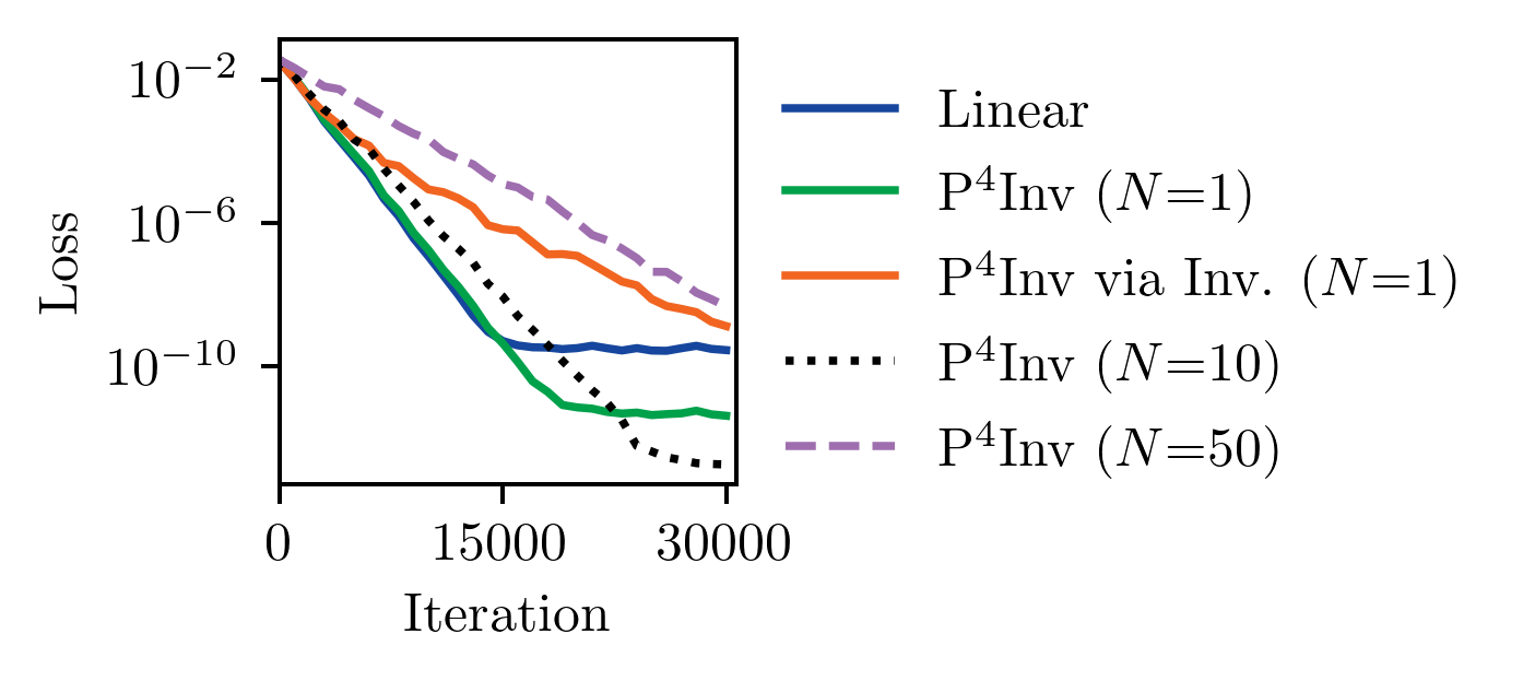
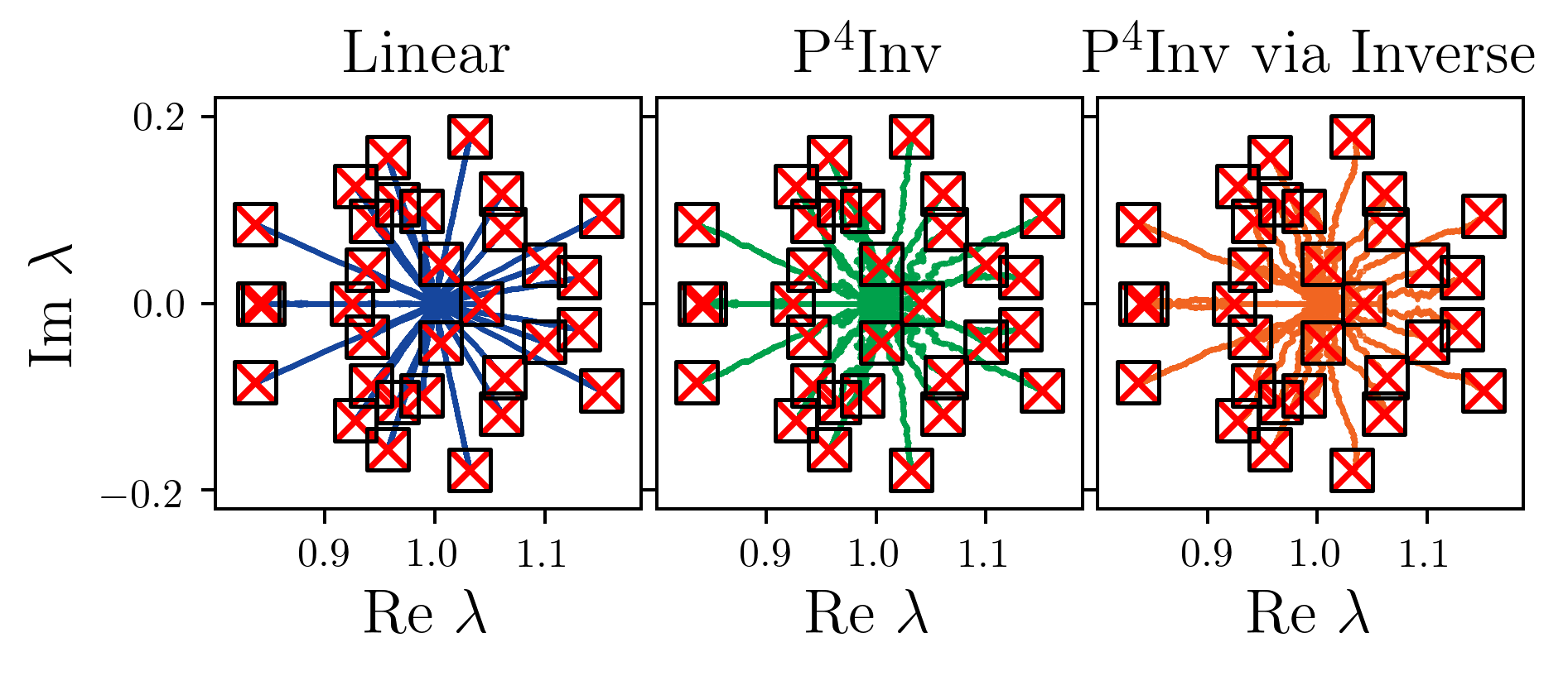
Figure 3: Training towards a 32-dimensional positive definite target matrix ${\bm{T}}$. Left: Losses during training. Right: Eigenvalues during training. Final eigenvalues are shown as red crosses. Eigenvalues of the target matrix are shown as black squares.

The first linear problem is a 32-dimensional positive definite matrix with eigenvalues close to 1. Figure 3 shows the evolution of eigenvalues and losses during training. All three methods of optimization successfully recovered the target matrix. While training P⁴Inv via the inverse led to slower convergence, the forward training of P⁴Inv converged in the same number of iterations as an unconstrained linear layer for a merge interval $N=1$. Increasing the merge interval to $N=10$ only affected the convergence minimally. Even for $N=50,$ the optimizer took only twice as many iterations as for an unconstrained linear layer.

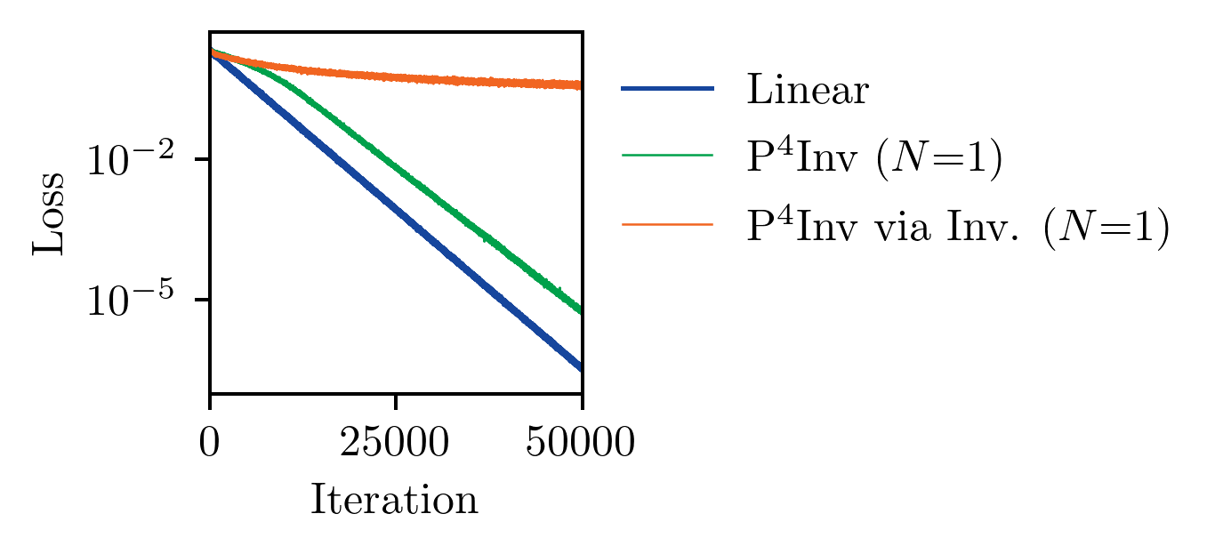
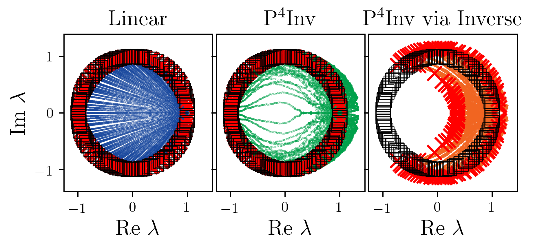
Figure 4: Training towards an orthogonal target matrix ${\bm{T}}\in\mathrm{SO}(128)$. Left: Losses during training. Right: Eigenvalues during training. Final eigenvalues are shown as red crosses. Eigenvalues of the target matrix are shown as black squares.

The second target matrix was a 128-dimensional special orthogonal matrix. As shown in Figure 4, the direct optimization converged to the target matrix in a linear fashion. In contrast, the matrices generated by the P⁴Inv update avoided the region around the origin. This detour led to a slower convergence in the initial phase of the optimization. Notably, the inverse stayed accurate up to 5 decimals throughout training. Training an inverse P⁴Inv was not successful for this example. This shows that the inverse P⁴Inv update can easily get stuck in local minima. This is not surprising as the elements of the inverse (equation 1) are parameterized by $\mathbb{R}^{2n}$-dimensional rational quadratic functions. When training against linear training data with a unique global optimum, the multimodality can prevent convergence. When training against more complex target data, the premature convergence was mitigated, see Appendix G. However, this result suggests that the efficiency of the optimization may be perturbed by very complex nonlinear parameterizations.

The final target matrix was ${\bm{T}}=-{\bm{I}}_{101},$ a matrix with determinant -1. In order to iteratively converge to the target matrix, the set of singular matrices has to be crossed. As expected, using a nonzero penalty parameter prevented the P⁴Inv update from converging to the target. However, when no penalty was applied, the matrix converged almost as fast as the usual linear training, see Figure 5. When the determinant approached zero, inversion became ill-conditioned and residues increased. However, after reaching the other side, the inverse was quickly recovered up to 5 decimal digits. Notably, the determinant also converged to the correct value despite never being explicitly corrected.

The favorable training efficiency encountered in those linear problems is surprising given the considerably reduced search space dimension. In fact, a subsequent rank-one parameterization of an MNIST classification task suggests that applications in nonlinear settings also converge as fast as standard MLPs in the initial phase, but slow down when approaching the optimum, see Appendix I.

4.3 2D Distributions

The next step was to assess the effectiveness of P⁴Inv layers in deep networks. This was particularly important to rule out a potentially harmful accumulation of rounding errors. Density estimation of common 2D toy distributions was performed by stacking P⁴Inv layers with Bent identities and their inverses. For comparison, an RNVP flow was constructed with the same number of tunable parameters as the P⁴Inv flow, see Appendix G for details.

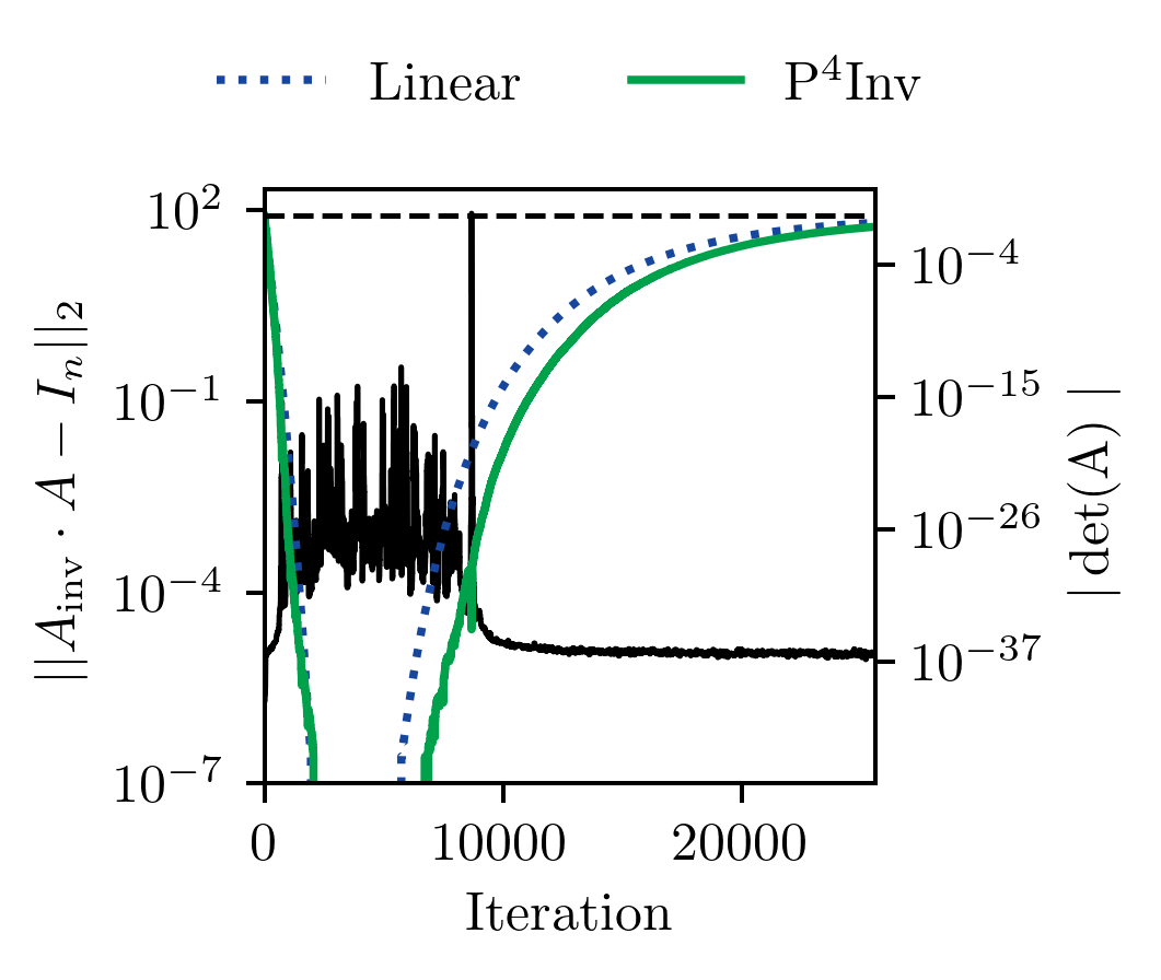
Figure 5: Training towards the matrix ${\bm{T}}=-{\bm{I}}_{101}$ using no penalty. Residue of inversion (black line) and absolute determinants of the standard linear and P⁴Inv layer. Both converge to the target in a similar number iterations (dashed line).

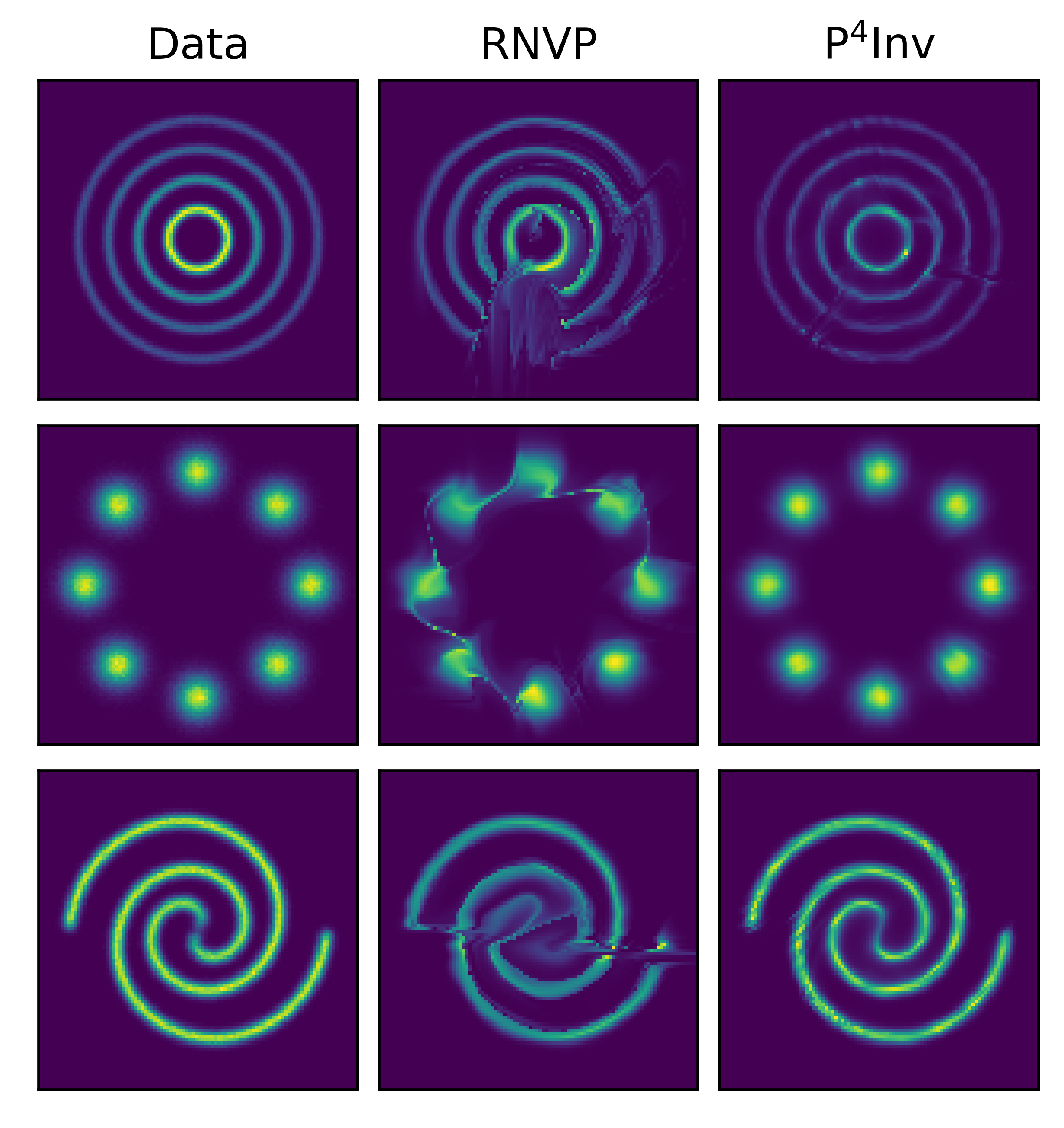
Figure 6: Density estimation for two-dimensional distributions from RealNVP (RNVP) and P⁴Inv networks with similar numbers of tunable parameters.

Figure 6 compares the generated distributions from the two models. The samples from the P⁴Inv model aligned favorably with the ground truth. In particular, they reproduced the multimodality of the data. In contrast to RNVP, P⁴Inv cleanly separated the modes, which underlines the favorable mixing achieved by general linear layers with elementwise nonlinear activations.

4.4 Boltzmann Generators of Alanine Dipeptide

Boltzmann generators (Noé et al., 2019) combine normalizing flows with statistical mechanics in order to draw direct samples from a given target density, e.g. given by a many-body physics system. This setup is ideally suited to assess the inversion of normalizing flows since the given physical potential energy defines the target density and thereby provides a quantitative measure for the sample quality. In molecular examples, specifically, the target densities are multimodal, contain singularities, and are highly sensitive to small perturbations in the atomic positions. Therefore, the generation of the 66-dimensional alanine dipeptide conformations is a highly nontrivial test for generative models.

The training efficiency and expressiveness of Boltzmann Generators (see Appendix E for details) were compared between pure RNVP baseline models as used in Noé et al. and models augmented by P⁴Inv swaps (see Section 3.4). The deep neural network architecture and training strategy are described in Appendix H. Both flows had 25 blocks as from Figure 9 in the appendix, resulting in 735,050 RNVP parameters. In contrast, the P⁴Inv blocks had only 9,000 tunable parameters. Due to this discrepancy and the depth of the network, we cannot expect dramatic improvements from adding P⁴Inv swaps. However, significant numerical errors in the inversion would definitely show in such a setup due to the highly sensitive potential energy.

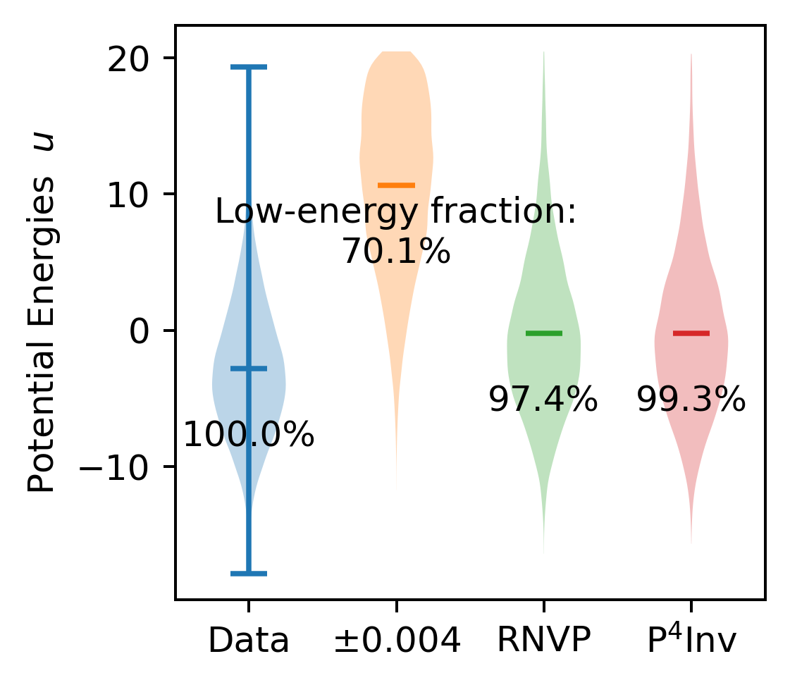
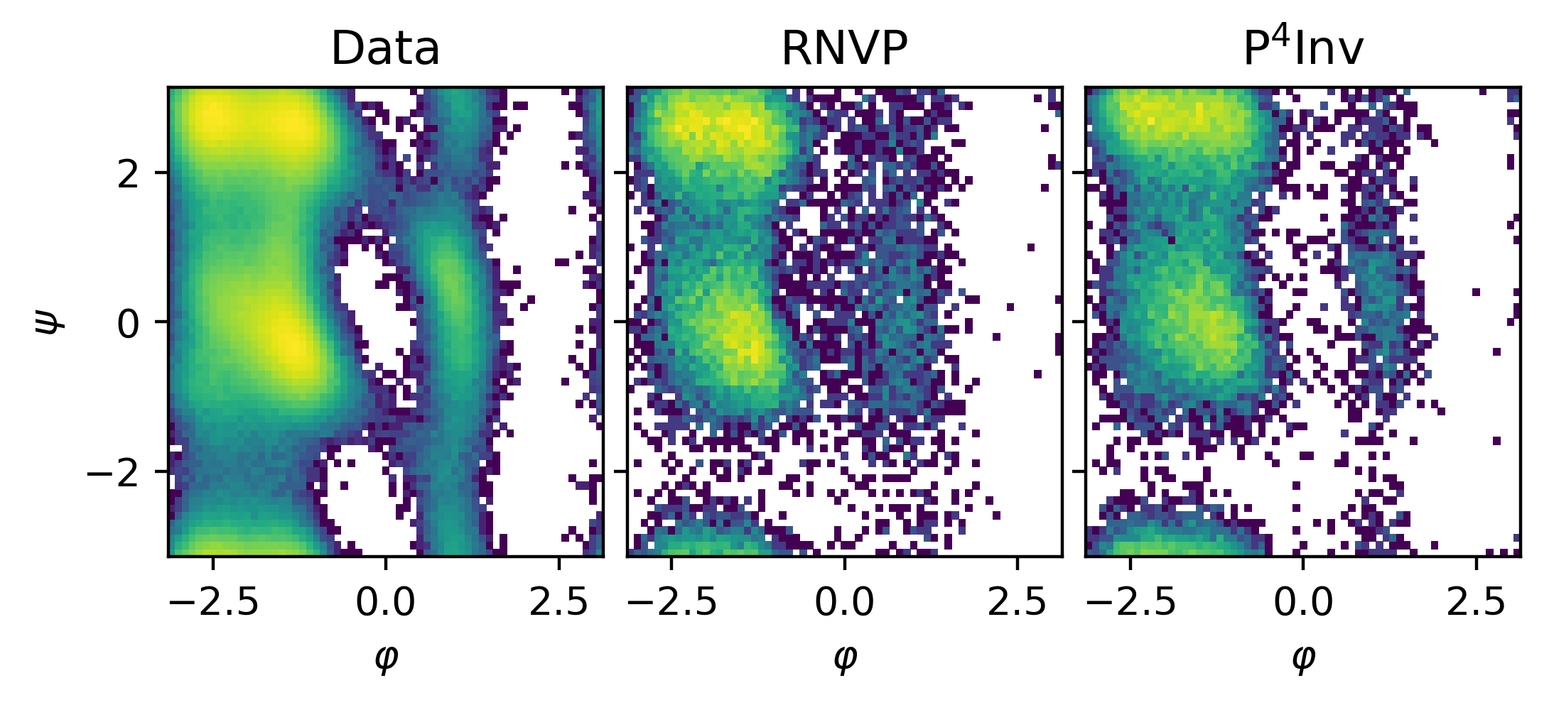
Figure 7: Left: Energy distributions of generated samples in dimensionless units of $k_{B}T$; the second (orange) violin plot shows energies when the training data was perturbed by normal distributed random noise with 0.004 nm standard deviation. The low-energy fraction for each column denotes the fraction of samples that had potential energy $u$ lower than the maximum energy from the training set ($\approx$ 20 $k_{B}T$). Right: Joint marginal distribution of the backbone torsions $\varphi$ and $\psi$: training data compared to samples from RealNVP Boltzmann generators with and without P⁴Inv swaps (denoted P⁴Inv and RNVP, respectively).

Figure 7 (left) shows the energy statistics of generated samples. To demonstrate the sensitivity of the potential energy, the training data was first perturbed by 0.004 nm (less than 1% of the total length of the molecule) and energies were evaluated for the perturbed data set. As a consequence, the mean of the potential energy distribution increased by 13 $k_{B}T$.

In comparison, the Boltzmann generators produced much more accurate samples. The energy distributions from RNVP and P⁴Inv blocks were only shifted upward by $\approx$ 2.6 $k_{B}T$ and rarely generated samples with infeasibly large energies. The performance of both models was comparable with slight advantages for models with P⁴Inv swaps. This shows that the P⁴Inv inverses remained intact during training. Finally, Figure 7 (right) shows the joint distribution of the two backbone torsions. Both Boltzmann generators reproduced the most important local minima of the potential energy. As in the 2D toy problems, the P⁴Inv layers provided a cleaner separation of modes.

5 Other Potential Applications of P⁴ Updates

Perturbation theorems are ubiquitous in mathematics and physics so that P⁴ updates will likely prove useful for retaining other properties of individual layers or neural networks as a whole. To this end, the P⁴ scheme in Section 3.1 is formulated in general terms. Orthogonal matrices may be parameterized in a similar manner to P⁴Inv through Givens rotations or double-Householder updates. Optimizers that constrain a joint property of multiple layers have previously been used to enforce Lipschitz bounds (Gouk et al. (2018), Yoshida & Miyato (2017)) and could also benefit from the present work. Applications in physics often rely on networks that obey the relevant physical invariances and equivariances (e.g. Köhler et al. (2020); Boyda et al. (2020); Kanwar et al. (2020); Hermann et al. (2020); Pfau et al. (2020); Rezende et al. (2019)). These properties might also be amenable to P⁴ training if suitable property-preserving perturbations can be defined.

6 Conclusions

We have introduced P⁴Inv updates, a novel algorithmic concept to preserve tractable inversion and determinant computation of linear layers using parameterized perturbations. Applications to normalizing flows proved the efficiency and accuracy of the inverses and determinants during training. A crucial aspect of the $P^{4}$ method is its decoupled merging step, which allows stable and efficient updates. As a consequence, the invertible linear P⁴Inv layers can approximate any well-conditioned regular matrix. This feature might open up new avenues to parameterize useful subsets of $\mathrm{GL}(n)$ through penalty functions. Since perturbation theorems like the rank-one update exist for many classes of linear and nonlinear functions, we believe that the P⁴ concept presents an efficient and widely applicable way of preserving desirable network properties during training.

Appendix A Sanity check for the Rank-One Update

Based on the matrix determinant lemma (equation 2) rank-one updates are ill-conditioned if the term $G:=1+{\bm{v}}^{T}{\bm{A}}_{\mathrm{inv}}{\bm{u}}$ vanishes. If such a perturbation is ever merged into the network parameters, the stored matrix determinant and inverse degrade and cannot be recovered. Therefore, merges are only accepted if the following conditions hold:

$$C_{\min}^{(0)}\leq\ln|G|\leq C_{\max}^{(0)}\qquad\mathrm{and}\qquad C_{\min}^{(1)}\leq\ln|G\det{\bm{A}}|\leq C_{\max}^{(1)}.$$

The constants $C_{\min}$ and $C_{\max}$ regularize the matrix ${\bm{A}}$ and its inverse ${\bm{A}}_{\mathrm{inv}},$ respectively, since $\ln|\det{\bm{A}}|=-\ln|\det{\bm{A}}_{\mathrm{inv}}|.$

The penalty function is also based on these constraints:

$$\begin{split}g({\bm{u}},{\bm{v}})=C_{p}\cdot\Big{(}&\mathrm{ReLU}^{2}\left(\ln|G|-C_{\max}\right)+\mathrm{ReLU}^{2}\left(C_{\min}-\ln|G|\right)\\ +&\mathrm{ReLU}^{2}\left(\ln|G\det{\bm{A}}|-C_{\max}\right)+\mathrm{ReLU}^{2}\left(C_{\min}-\ln|G\det{\bm{A}}|\right)\Big{)}\end{split}$$

with a penalty parameter $C_{p}.$ For the experiments in this work, we used $C_{\min}=-2$, $C_{\max}=15$, $C_{\min}^{(0)}=-6$, $C_{\max}^{(0)}=\inf$, $C_{\min}^{(1)}=-2.5$, and $C_{\max}^{(1)}=15.5$.

Appendix B Implementation of P⁴Inv Layers

In practice, the P⁴Inv layer stores the current inverse ${\bm{A}}_{\mathrm{inv}}\approx{\bm{A}}^{-1}$ and determinant alongside ${\bm{A}}.$ The forward pass of an input vector ${\bm{x}}$ can be computed efficiently by first computing ${\bm{u}}^{T}{\bm{x}}$ and then adding ${\bm{v}}{\bm{u}}^{T}{\bm{x}}$ to ${\bm{A}}{\bm{x}}$. The inverse pass can be similarly structured to avoid any matrix multiplies.

Note that P⁴ training can straightforwardly be applied to only a part of the network parameters. In this case, all other parameters are directly optimized without the perturbation proxy and the gradient of the loss function $J$ is composed of elements from $\partial J/\partial{\bm{\mathsfit{B}}}$ and $\partial J/\partial{\bm{\mathsfit{A}}}.$ Furthermore, the perturbation of parameters and evaluation of the perturbed model can sometimes be done more efficiently in one step. Also, the merging step from equation 3 and equation 4 can additionally be augmented to rectify numerical errors made during optimization.

In order to allow crossings of otherwise inaccessible regions of the parameter space the merging step was accepted every $N_{\mathrm{force}}$ merges, even if the determinant was poorly conditioned. If ${\bm{u}}$ or ${\bm{v}}$ ever contain non-numeric values, merging steps were rejected and the perturbation is reset without performing a merge.

Appendix C Normalizing Flows

A Normalizing flow is a learnable bijection $f\colon\mathbb{R}^{n}\rightarrow\mathbb{R}^{n}$ which transforms a simple base distribution $p(z)$, by first sampling $z\sim p(z)$, and then transforming into $x=f(z)$. According to the change of variables, the transformed sample $x$ has the density:

$$q(x)=p\left(f^{-1}(x)\right)\left|\det\mathbf{J}_{f^{-1}}(x)\right|.$$

Given a target distribution $\rho(x)$, this tractable density allows minimizing the reverse Kullback-Leibler (KL) divergence $\mathcal{D}_{\text{KL}}\left[q(x)\|\rho(x)\right],$ e.g., if $\rho(x)$ is known up to a normalizing constant, or the forward KL divergence $\mathcal{D}_{\text{KL}}\left[\rho(x)\|q(x)\right],$ if having access to samples from $\rho(x)$.

Appendix D Coupling Layers

Maintaining invertibility and computing the inverse and its Jacobian is a challenge, if $f$ could be an arbitrary function. Thus, it is common to decompose $f$ in a sequence of coupling layers

$$f=g^{(1)}\circ\mathcal{S}^{(1)}\circ\ldots g^{(K)}\circ\mathcal{S}^{(K)}.$$

Each $g^{(k)}$ is constrained to the form $g^{(k)}(x)=T^{(k)}(x_{1},x_{2})\oplus x_{2}$, where $x=x_{1}\oplus x_{2},~{}x_{1}\in\mathbb{R}^{m}$ and $x_{2}\in\mathbb{R}^{n-m}$. Here $T^{(k)}\colon\mathbb{R}^{m}\times\mathbb{R}^{n-m}\rightarrow\mathbb{R}^{m}$ is a point-wise transformation, which is invertible in its first component given a fixed $x_{2}$. Possible implementations include simple affine transformations (Dinh et al., 2014; 2016) as well as complex transformations based on splines (Müller et al., 2019; Durkan et al., 2019). Each $g^{(k)}$ thus has a block-triangular Jacobian matrix

$$\mathbf{J}_{g^{(k)}}=\left[\begin{array}[]{cc}\mathbf{J}_{T^{(k)}}&\mathbf{M}^{(k)}\\ \mathbf{0}&\mathbf{I}_{m\times m}\end{array}\right],$$

where $\mathbf{J}_{T^{(k)}}$ is a $(n-m)\times(n-m)$ diagonal matrix. The layers $\mathcal{S}^{(k)}$ take care of achieving a mixing between coordinates and are usually represented as simple swaps

$$\mathcal{S}^{(k)}=\left[\begin{array}[]{cc}\mathbf{0}&\mathbf{I}_{n-m\times n-m}\\ \mathbf{I}_{m\times m}&\mathbf{0}\end{array}\right].$$

The total log Jacobian of $f_{\theta}$ is then given by

$$\log\det\mathbf{J}_{f_{\theta}}=\sum_{k=1}^{K}\text{tr}\left[\log\left(\mathbf{J}_{T^{(k)}}\right)\right]+\log\det\mathcal{S}^{(k)},$$

where $\log\det\mathcal{S}^{(k)}=0$ when $\mathcal{S}^{(k)}$ is given by the simple swaps above.

Appendix E Boltzmann Generators

Boltzmann Generators (Noé et al., 2019) are generative neural networks that sample with respect to a known target energy, as for example given by molecular force fields. The potential energy $u:\mathbb{R}^{3n}\rightarrow{\mathbb{R}}$ of such systems is a function of the atom positions ${\mathbf{x}}.$ The corresponding probability of each configuration ${\mathbf{x}}$ is given by the Boltzmann distribution $p_{x}({\mathbf{x}})=\exp(-\beta u({\mathbf{x}}))/Z,$ where $\beta=1/(k_{B}T)$ is inverse temperature with the Boltzmann constant $k_{B}.$ The normalization constant $Z$ is generally not known.

The generation uses a normalizing flow and training is performed via a combination of density estimation and energy-based training. Concretely, the following loss function is minimized

$$J({\bm{A}})=w_{l}J_{l}({\bm{A}})+w_{e}J_{e}({\bm{A}}),$$ (6)

where $w_{l}+w_{e}=1$ denote weighting factors between density estimation and energy-based training. The maximum likelihood and KL divergence in equation 6 are defined respectively as

$$J_{l} =\mathbb{E}_{{\mathbf{x}}\sim p_{x}}\left[\frac{1}{2}\|F_{xz}({\mathbf{x}};{\bm{A}})\|^{2}-\ln R_{xz}({\mathbf{x}};{\bm{A}})\right]\quad\mathrm{and}$$

$$J_{e} =\mathbb{E}_{{\mathbf{z}}\sim p_{z}}\left[u(F_{zx}({\mathbf{z}};{\bm{A}}))-\ln R_{zx}({\mathbf{z}};{\bm{A}})\right].$$

As an example, we train a model for alanine dipeptide, a molecule with 22 atoms, in water. Water is represented by an implicit solvent model. This system was previously used in Wu et al. (2020). Training data was generated using MD simulations at 600K to sample all metastable regions.

Appendix F Training of Linear Toy Problems

The P⁴Inv layers were trained using a stochastic gradient descent optimizer with a learning rate of $10^{-2}$ and the hyperparameters from Table 1. The matrices were initialized with the identity.

Table 1: Hyperparameters for linear toy problems

Problem (Dimension)	$N$	$N_{\mathrm{force}}$	$N_{\mathrm{correct}}$	Penalty $C_{0}$
Positive Definite (32)	1, 10, 50	10	50	0.1
Orthogonal (128)	1	10	50	0.1
$-{\bm{I}}$ (101)	1	10	50	0.0

Appendix G Training of 2D Distributions

The P⁴Inv layers used for 2D distributions were composed of blocks containing

1. a P⁴Inv layer with bias (2D),

2. an elementwise Bent identity,

3. another P⁴Inv layer with bias (2D), and

4. an inverse elementwise Bent identity.

100 of these blocks were stacked resulting in 1200 tunable parameters (counting elements of ${\bm{u}}$ and ${\bm{v}}$). P⁴Inv training was performed with $N=10,$ $N_{\mathrm{force}}=10$ and $N_{\mathrm{correct}}=50$. No penalty was used. Matrices were initialized with the identity ${\bm{I}}_{2}.$

The RealNVP network used for comparison was composed of five RealNVP layers. The additive and multiplicative conditioner networks used dense nets with two 6-dimensional hidden layers each and $\tanh$ activation functions, respectively. This resulted in a total of 1230 parameters.

The examples are taken from Grathwohl et al. (2018). Priors were two-dimensional standard normal distributions. Adam optimization was performed for 8 epochs of 20000 steps and with a batch size of 200. The initial learning rate was $5\cdot 10^{-3}$ and decreased by a factor of $0.5$ in each epoch. After each merging step, the metaparameters of the Adam optimizer were reset to their initial state.

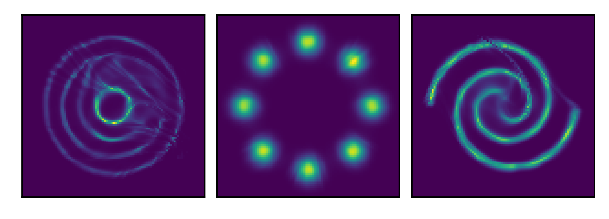
Figure 8: Samples from P⁴Inv training via the inverse.

Figure 8 complements Figure 6 by showing samples from a network with only inverse P⁴Inv blocks. While the samples are worse than with forward blocks, the distributions are still well represented. This result indicates that the premature convergence encountered for linear test problems is a lesser problem in nonlinear problems and deep architectures.

Appendix H Training of Boltzmann Generators

Figure 9: Neural network blocks used in the Boltzmann generator application. The baseline architecture is a normalizing flow composed of Real NVP (RNVP) coupling blocks. RNVP uses input from two channels $x_{1}$ and $x_{2}.$ The input from the first channel is left untouched, $y_{1}=x_{1},$ while the output $y_{2}$ from the second channel is conditioned on the first channel through two neural networks $t$ and $s$. Each block of the baseline model contains two RNVP blocks and two swapping steps that are bracketed by splitting and concatenation (cat) of the data. Instead of the swapping steps, the P⁴Inv model uses invertible linear layers that are trained through P⁴ updates.

The normalizing flows in Boltzmann generators were composed of the blocks shown in Figure 9 and a mixed coordinate transform as defined in Noé et al. (2019). The test problem was taken from Dibak et al. (2020). RNVP layers contained two 60-dimensional hidden layers each and ReLU and $\tanh$ activation functions for both $t$ and $s$, respectively. The baseline model consisted of blocks of alternated RNVP blocks and swaps. The P⁴Inv model used invertible linear layers instead of the swapping of input channels in the baseline model. The computational overhead due to this change was negligible. RNVP parameters were optimized directly as usual and only the P⁴Inv layers are affected by the P⁴ updates. Merging was performed every $N=100$ steps with $N_{\mathrm{force}}=10$ and $N_{\mathrm{correct}}=50$. No penalty was used, i.e. $C_{0}=0.0$. The P⁴Inv matrices were initialized with the reverse permutation, i.e. ${A}_{ij}=\delta_{i(n-j)}.$

Density estimation with Adam was performed for 40,000 optimization steps with a batch size of 256 and a learning rate of $10^{-3}.$ A short energy-based training epoch was appended for 2000 steps with a learning rate of $10^{-5}$ and $w_{e}/w_{l}=0.05.$ After each merging step, the metaparameters of the Adam optimizer were reset to their initial state for all P⁴Inv parameters.

Appendix I MNIST Classification via Rank-one Updates

Compared to fully-connected multi-layer perceptrons (MLP), rank-one updates reduce the number of independent trainable parameters per layer from $m\cdot n$ to $m+n-1,$ where $m$ and $n$ are the input and output dimension, respectively. It is therefore useful to study how the reduced search space dimension affects the training efficiency in a nonlinear setup. To this end, non-invertible classifier MLPs were trained on MNIST with an unrestricted search space as well as through rank-one updates. The original network was composed of two convolutional layers, two dropout layers, and two linear layers. In P⁴ training, the two linear layers (dimensions 9216$\times$128 and 128$\times$10) were trained through rank-one updates which were merged in every iteration ($N=1$). Naturally, this training did not involve any inverse or determinant updates. A vanilla SGD optimizer was used with various learning rates.

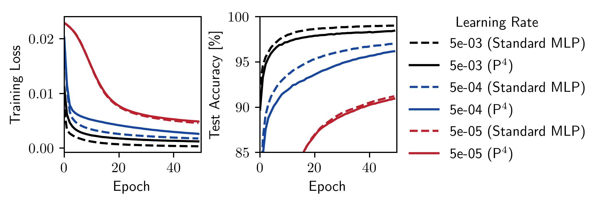
Figure 10: Training loss and test accuracy during MNIST training with a vanilla SGD optimizer averaged over ten replicas. Standard multilayer perceptrons (MLP) are compared with rank-one updates.

Figure 10 shows the training loss and test accuracy during training. As for the linear problems from the previous subsection, the training efficiency was virtually unaffected during the first phase of the optimization, i.e. when the descent direction did not change significantly between subsequent iterations. However, as the descent direction became more noisy in the vicinity of the optimum, the training with rank-one updates became less efficient.

References

- Absil et al. (2009) P. A. Absil, R. Mahony, and R. Sepulchre. Optimization algorithms on matrix manifolds. Princeton University Press, 2009. ISBN 9780691132983. doi: 10.1515/9781400830244.
- Behrmann et al. (2019) Jens Behrmann, Will Grathwohl, Ricky T. Q. Chen, David Duvenaud, and Joern-Henrik Jacobsen. Invertible residual networks. In Proceedings of the 36th International Conference on Machine Learning, volume 97 of Proceedings of Machine Learning Research, pp. 573–582, Long Beach, California, USA, 2019. PMLR. URL http://proceedings.mlr.press/v97/behrmann19a.html.
- Boyda et al. (2020) Denis Boyda, Gurtej Kanwar, Sébastien Racanière, Danilo Jimenez Rezende, Michael S Albergo, Kyle Cranmer, Daniel C Hackett, and Phiala E Shanahan. Sampling using gauge equivariant flows. arXiv preprint arXiv:2008.05456, 2020.
- Chen et al. (2018) Tian Qi Chen, Yulia Rubanova, Jesse Bettencourt, and David K Duvenaud. Neural ordinary differential equations. In Advances in neural information processing systems, pp. 6571–6583, 2018.
- Chen et al. (2019) Tian Qi Chen, Jens Behrmann, David K Duvenaud, and Jörn-Henrik Jacobsen. Residual flows for invertible generative modeling. In Advances in Neural Information Processing Systems, pp. 9913–9923, 2019.
- Choromanski et al. (2020) Krzysztof Choromanski, David Cheikhi, Jared Davis, Valerii Likhosherstov, Achille Nazaret, Achraf Bahamou, Xingyou Song, Mrugank Akarte, Jack Parker-Holder, Jacob Bergquist, Yuan Gao, Aldo Pacchiano, Tamas Sarlos, Adrian Weller, and Vikas Sindhwani. Stochastic flows and geometric optimization on the orthogonal group. In 37th International Conference on Machine Learning (ICML 2020), 2020. URL https://arxiv.org/abs/2003.13563.
- De Cao et al. (2019) Nicola De Cao, Ivan Titov, and Wilker Aziz. Block neural autoregressive flow. In Conference on Uncertainty in Artificial Intelligence (UAI), 2019. URL https://arxiv.org/abs/1904.04676.
- Dibak et al. (2020) Manuel Dibak, Leon Klein, and Frank Noé. Temperature-steerable flows. Machine Learning and the Physical Sciences, Workshop at the 34th Conference on Neural Information Processing Systems (NeurIPS), 2020.
- Dinh et al. (2014) Laurent Dinh, David Krueger, and Yoshua Bengio. Nice: Non-linear independent components estimation. arXiv preprint arXiv:1410.8516, 2014.
- Dinh et al. (2016) Laurent Dinh, Jascha Sohl-Dickstein, and Samy Bengio. Density estimation using real nvp. arXiv preprint arXiv:1605.08803, 2016.
- Durkan et al. (2019) Conor Durkan, Artur Bekasov, Iain Murray, and George Papamakarios. Neural spline flows. In Advances in Neural Information Processing Systems, pp. 7509–7520, 2019.
- Falorsi et al. (2019) Luca Falorsi, Pim de Haan, Tim R. Davidson, and Patrick Forré. Reparameterizing distributions on lie groups. In Proceedings of the 22nd International Conference on Artificial Intelligence and Statistics (AISTATS) 2019, volume 89 of Proceedings of Machine Learning Research, pp. 3244–3253. PMLR, 2019. URL http://proceedings.mlr.press/v89/falorsi19a.html.
- Germain et al. (2015) Mathieu Germain, Karol Gregor, Iain Murray, and Hugo Larochelle. Made: Masked autoencoder for distribution estimation. In International Conference on Machine Learning, pp. 881–889, 2015.
- Golinski et al. (2019) Adam Golinski, Mario Lezcano-Casado, and Tom Rainforth. Improving normalizing flows via better orthogonal parameterizations. In ICML Workshop on Invertible Neural Networks and Normalizing Flows, 2019.
- Gouk et al. (2018) Henry Gouk, Eibe Frank, Bernhard Pfahringer, and Michael Cree. Regularisation of Neural Networks by Enforcing Lipschitz Continuity. arXiv preprint arXiv:1804.04368, 2018. URL http://arxiv.org/abs/1804.04368.
- Grathwohl et al. (2018) Will Grathwohl, Ricky TQ Chen, Jesse Bettencourt, Ilya Sutskever, and David Duvenaud. Ffjord: Free-form continuous dynamics for scalable reversible generative models. In 7th International Conference on Learning Representations (ICLR), 2018. URL https://arxiv.org/abs/1810.01367.
- Gresele et al. (2020) Luigi Gresele, Giancarlo Fissore, Adrián Javaloy, Bernhard Schölkopf, and Aapo Hyvärinen. Relative gradient optimization of the jacobian term in unsupervised deep learning. In 34th Conference on Neural Information Processing Systems (NeurIPS 2020), 2020. URL https://arxiv.org/abs/2006.15090.
- Helfrich et al. (2018) Kyle Helfrich, Devin Willmott, and Qiang Ye. Orthogonal recurrent neural networks with scaled cayley transform. In International Conference on Machine Learning, pp. 1969–1978. PMLR, 2018.
- Hermann et al. (2020) Jan Hermann, Zeno Schätzle, and Frank Noé. Deep-neural-network solution of the electronic Schrödinger equation. Nat. Chem., 12(10):891–897, 2020. ISSN 17554349. doi: 10.1038/s41557-020-0544-y.
- Hoogeboom et al. (2019) Emiel Hoogeboom, Rianne van den Berg, and Max Welling. Emerging convolutions for generative normalizing flows. In International conference on machine learning, 2019. URL https://arxiv.org/abs/1901.11137.
- Hoogeboom et al. (2020) Emiel Hoogeboom, Victor Garcia Satorras, Jakub M Tomczak, and Max Welling. The convolution exponential and generalized sylvester flows. In 34th Conference on Neural Information Processing Systems (NeurIPS 2020), 2020. URL https://papers.nips.cc/paper/2020/file/d3f06eef2ffac7faadbe3055a70682ac-Paper.pdf.
- Huang et al. (2018) Chin-Wei Huang, David Krueger, Alexandre Lacoste, and Aaron Courville. Neural autoregressive flows. arXiv preprint arXiv:1804.00779, 2018.
- Kanwar et al. (2020) Gurtej Kanwar, Michael S. Albergo, Denis Boyda, Kyle Cranmer, Daniel C. Hackett, Sébastien Racanière, Danilo Jimenez Rezende, and Phiala E. Shanahan. Equivariant flow-based sampling for lattice gauge theory. Phys. Rev. Lett., 125:121601, 2020. doi: 10.1103/PhysRevLett.125.121601. URL https://link.aps.org/doi/10.1103/PhysRevLett.125.121601.
- Karami et al. (2019) Mahdi Karami, Dale Schuurmans, Jascha Sohl-Dickstein, Laurent Dinh, and Daniel Duckworth. Invertible convolutional flow. In Advances in Neural Information Processing Systems, pp. 5635–5645, 2019.
- Kingma & Dhariwal (2018) Durk P Kingma and Prafulla Dhariwal. Glow: Generative flow with invertible 1x1 convolutions. In Advances in neural information processing systems, pp. 10215–10224, 2018.
- Köhler et al. (2020) Jonas Köhler, Leon Klein, and Frank Noé. Equivariant flows: exact likelihood generative learning for symmetric densities. arXiv preprint arXiv:2006.02425, 2020.
- Lezcano-Casado (2019) Mario Lezcano-Casado. Trivializations for gradient-based optimization on manifolds. In 33rd Conference on Neural Information Processing Systems (NeurIPS 2019), volume 32, pp. 9157–9168, 2019. URL https://proceedings.neurips.cc/paper/2019/file/1b33d16fc562464579b7199ca3114982-Paper.pdf.
- Lezcano-Casado (2020) Mario Lezcano-Casado. Curvature-dependant global convergence rates for optimization on manifolds of bounded geometry. arXiv preprint arXiv:2008.02517, 2020.
- Lezcano-Casado & Martínez-Rubio (2019) Mario Lezcano-Casado and David Martínez-Rubio. Cheap orthogonal constraints in neural networks: A simple parametrization of the orthogonal and unitary group. In Proceedings of the 36th International Conference on Machine Learning, volume 97, pp. 3794–3803. PMLR, 2019. URL http://proceedings.mlr.press/v97/lezcano-casado19a.html.
- Louizos & Welling (2017) Christos Louizos and Max Welling. Multiplicative normalizing flows for variational bayesian neural networks. In Proceedings of the 34th International Conference on Machine Learning-Volume 70, pp. 2218–2227, 2017.
- Meng et al. (2020) Chenlin Meng, Yang Song, Jiaming Song, and Stefano Ermon. Gaussianization flows. arXiv preprint arXiv:2003.01941, 2020.
- Mhammedi et al. (2017) Zakaria Mhammedi, Andrew Hellicar, Ashfaqur Rahman, and James Bailey. Efficient orthogonal parametrisation of recurrent neural networks using householder reflections. In International Conference on Machine Learning, pp. 2401–2409. PMLR, 2017.
- Müller et al. (2019) Thomas Müller, Brian McWilliams, Fabrice Rousselle, Markus Gross, and Jan Novák. Neural importance sampling. ACM Trans. Graph., 38(5), 2019. ISSN 0730-0301. URL https://doi.org/10.1145/3341156.
- Noé et al. (2019) Frank Noé, Simon Olsson, Jonas Köhler, and Hao Wu. Boltzmann generators: Sampling equilibrium states of many-body systems with deep learning. Science, 365(6457):eaaw1147, 2019.
- Papamakarios et al. (2017) George Papamakarios, Theo Pavlakou, and Iain Murray. Masked autoregressive flow for density estimation. In Advances in Neural Information Processing Systems, pp. 2338–2347, 2017.
- Papamakarios et al. (2019) George Papamakarios, Eric Nalisnick, Danilo Jimenez Rezende, Shakir Mohamed, and Balaji Lakshminarayanan. Normalizing flows for probabilistic modeling and inference. arXiv preprint arXiv:1912.02762, 2019.
- Pevny et al. (2020) Tomas Pevny, Vasek Smidl, Martin Trapp, Ondrej Polacek, and Tomas Oberhuber. Sum-product-transform networks: Exploiting symmetries using invertible transformations. arXiv preprint arXiv:2005.01297, 2020.
- Pfau et al. (2020) David Pfau, James S. Spencer, Alexander G. D. G. Matthews, and W. M. C. Foulkes. Ab initio solution of the many-electron schrödinger equation with deep neural networks. Phys. Rev. Research, 2:033429, 2020. doi: 10.1103/PhysRevResearch.2.033429. URL https://link.aps.org/doi/10.1103/PhysRevResearch.2.033429.
- Rezende & Mohamed (2015) Danilo Rezende and Shakir Mohamed. Variational inference with normalizing flows. In Proceedings of the 32nd International Conference on Machine Learning, volume 37, pp. 1530–1538, 2015. URL http://proceedings.mlr.press/v37/rezende15.html.
- Rezende et al. (2019) Danilo Jimenez Rezende, Sébastien Racanière, Irina Higgins, and Peter Toth. Equivariant hamiltonian flows. arXiv preprint arXiv:1909.13739, 2019.
- Shalit & Chechik (2014) Uri Shalit and Gal Chechik. Coordinate-descent for learning orthogonal matrices through Givens rotations. In 31st International Conference on Machine Learning (ICML 2014), volume 1, pp. 833–845, 2014. ISBN 9781634393973. URL http://arxiv.org/abs/1312.0624.
- Soleymani (2014) Fazlollah Soleymani. A fast convergent iterative solver for approximate inverse of matrices. Numerical Linear Algebra with Applications, 21(3):439–452, 2014.
- Tabak & Turner (2013) Esteban G Tabak and Cristina V Turner. A family of nonparametric density estimation algorithms. Communications on Pure and Applied Mathematics, 66(2):145–164, 2013.
- Tabak et al. (2010) Esteban G Tabak, Eric Vanden-Eijnden, et al. Density estimation by dual ascent of the log-likelihood. Communications in Mathematical Sciences, 8(1):217–233, 2010.
- Tomczak & Welling (2016) Jakub M Tomczak and Max Welling. Improving variational auto-encoders using householder flow. arXiv preprint arXiv:1611.09630, 2016.
- Van Den Berg et al. (2018) Rianne Van Den Berg, Leonard Hasenclever, Jakub M. Tomczak, and Max Welling. Sylvester normalizing flows for variational inference. In 34th Conference on Uncertainty in Artificial Intelligence 2018, UAI 2018, 34th Conference on Uncertainty in Artificial Intelligence 2018, UAI 2018, pp. 393–402, 2018. 34th Conference on Uncertainty in Artificial Intelligence 2018, UAI 2018 ; Conference date: 06-08-2018 Through 10-08-2018.
- van den Oord et al. (2018) Aaron van den Oord, Yazhe Li, Igor Babuschkin, Karen Simonyan, Oriol Vinyals, Koray Kavukcuoglu, George van den Driessche, Edward Lockhart, Luis Cobo, Florian Stimberg, Norman Casagrande, Dominik Grewe, Seb Noury, Sander Dieleman, Erich Elsen, Nal Kalchbrenner, Heiga Zen, Alex Graves, Helen King, Tom Walters, Dan Belov, and Demis Hassabis. Parallel WaveNet: Fast high-fidelity speech synthesis. In Proceedings of the 35th International Conference on Machine Learning, volume 80 of Proceedings of Machine Learning Research, pp. 3918–3926, 2018. URL http://proceedings.mlr.press/v80/oord18a.html.
- Wu et al. (2020) Hao Wu, Jonas Köhler, and Frank Noé. Stochastic normalizing flows. arXiv preprint arXiv:2002.06707, 2020.
- Yoshida & Miyato (2017) Yuichi Yoshida and Takeru Miyato. Spectral norm regularization for improving the generalizability of deep learning, 2017.
- Zhang et al. (2018) Linfeng Zhang, Lei Wang, et al. Monge-ampere flow for generative modeling. arXiv preprint arXiv:1809.10188, 2018.