Chance-constrained Stochastic MPC of Astlingen Urban Drainage Benchmark Network

Abstract

In urban drainage systems (UDS), a proven method for reducing the combined sewer overflow (CSO) pollution is real-time control (RTC) based on model predictive control (MPC). MPC methodologies for RTC of UDSs in the literature rely on the computation of the optimal control strategies based on deterministic rain forecast. However, in reality, uncertainties exist in rainfall forecasts which affect severely accuracy of computing the optimal control strategies. Under this context, this work aims to focus on the uncertainty associated with the rainfall forecasting and its effects. One option is to use stochastic information about the rain events in the controller; in the case of using MPC methods, the class called stochastic MPC is available, including several approaches such as the chance-constrained MPC method. In this study, we apply stochastic MPC to the UDS using the chance-constrained method. Moreover, we also compare the operational behavior of both the classical MPC with perfect forecast and the chance-constrained MPC based on different stochastic scenarios of the rain forecast. The application and comparison have been based on simulations using a SWMM model of the Astlingen urban drainage benchmark network.

1 Introduction

Regarding the state-of-the-art during the last couple of decades, Model Predictive Control (MPC) [1] has been proved beneficial for the optimal operation of urban drainage systems (UDS)[2]-[10]. Those studies use different types of modeling and optimization techniques to compute the best control actions, based on models and forecasts, which are subject to uncertainty. However, up to now, most of the MPC applications of UDS are based on deterministic rain forecasts without considering uncertainties, which may risk in introducing sub-optimal or undesired behaviors to the MPC solutions [2]-[16]. For a more realistic scenario, uncertainty has to be considered as a part of the UDS. The way how the uncertainty is treated by the control, becomes an important design decision: using a stochastic approach, or robustly operating on worst-case assumptions.

While the basic formulation of MPC is deterministic, how to handle uncertainty in MPC has been researched for many years [17]-[27]. This has resulted in several different methods for handling uncertainty divided into two categories; the group of the methods known collectively as robust MPC[24]-[27], and the group of methods known as stochastic MPC[17]-[24]. The first group essentially considers the worst-case scenario and operates conservatively so that the solution is optimal for all possible realizations of the uncertainty. The second group addresses the uncertainty by using knowledge about the uncertainty, such as its distribution to only take the statistical likely scenarios into account for the control.

In this work, we will focus on a method from the group of stochastic methods known as chance-constrained MPC (CC-MPC)[17]-[20] to operate the UDS in order to reduce pollution to the receiving waters through minimization of the combined sewer overflows (CSO). Given that the CSOs are purely dependent on the volumes and flows of the system; the overflow constraints are intrinsically feasible and probabilistic insenstive, when CC-MPC is applied directly. We will therefore use the revised CC-MPC formulation[17] in this work.

In our previous work[4], an MPC methodology was implemented and tested on a SWMM model of the Astlingen urban drainage benchmark network [28], where the goal was to minimize the CSOs volume of the system, while maximizing the amount of treated wastewater by the wastewater treatment plant (WWTP). We obtained good results from this, in comparison with other real-time control strategies. In this paper, we return to the Astlingen urban drainage system for applying stochastic MPC using chance-constrained method regarding the uncertainty of rainfall forecast, and comparing the performance of CC-MPC with uncertain forecasts against the performance of the deterministic MPC with a perfect forecast. The key performance indexes considered are the CSO volume, and the volume received by the WWTP.

In this paper, the following mathematical notations are used. $\overline{f}$ indicates the maximum of a given function $f(x)$, $\beta$ represents the volume-flow coefficient[29], and bold font is used to indicate vectors. The formulation $\|\textbf{x}\|_{A}^{2}=\textbf{x}^{T}A\textbf{x}$ is the weighted quadratic norm of x. The superscript u indicates control variables, superscript w indicates CSO elements, and the superscripts in and out indicate inflow and outflow related flow, respectively. The letters V and q indicate variables of volume and flow respectively, while the variables written with w are inflows from catchments. The notation $\Delta T$ and the subscript k represent the sampling time of the system and the sample number respectively.

2 Internal model of the Astlingen Benchmark Network

The Astlingen urban drainage network consists of six tanks and a single outflow towards a WWTP (see Figure 1). In between and upstream of the tanks there are pipes of varying lengths, causing flow delays in the system. The system also consists of four pipes with CSO capabilities. The control variables of the system are the outflow of tanks 2, 3, 4, and 6. The desired operation of the system is to have the least amount of CSO as possible, and secondly having the largest amount of wastewater being sent to the WWTP. For designing an MPC controller for the system, an internal model describing the dynamics and constraints of this system is required, typically a simplified model of the system capturing the main dynamic behaviours is used.

From Figure 1, it is clear that the system can be deduced to be uncontrollable (passive) in the sections upstream the tanks; therefore, the internal model will be limited to only covering the tanks of the system. The internal model is constructed with the same modular approach as used in previous works[4]. In the internal model, the CSO are treated as optimization variables through a penalty approach[2]. The elements of the internal model consist of the following parts: linear reservoir tanks and pipes with delays that are described below.

In CC-MPC, the internal model of the deterministic MPC mentioned above is extended with a process equation of the variance of the dynamics, while the dynamics are replaced with the expectation of the dynamics. The constraints are reformulated either as the expectation of the constraint or as a probabilistic version of the constraints. The prior is in general used for equality constraints, while the latter is used for inequality constraints.

In this work, the run-off flows ($w$, covering runoff and passive flows) generated by forecasted rainfalls are the disturbance, involving uncertainty. We will assume this uncertainty to follow a normal distribution, which is commonly used to interpret fluctuations in measured or forcasted variables[30, 31]. Then, for uncertainties following a normal distribution, the probabilistic constraints can be written deterministically as shown in (1), using the expectation $E\{x\}$ and standard deviation $\sigma\{x\}$ of the stochastic variable X, as well as the quantile function $\Phi^{-1}(x)$ of the standard normal distribution on the desired probability confidence level $\gamma$

$$Pr(X\leq x)\geq\gamma\Leftrightarrow x\geq E\{X\}+\sigma\{X\}\Phi^{-1}(\gamma)$$ (1)

Furthermore, the only sources of uncertainty considered in the formulation of the internal model for the CC-MPC are the initial states of the system and the inflow from the run-off sources such as catchments. It is further assumed that the different sources of uncertainties are independently distributed, in both spatial and temporal sense.

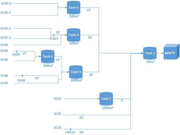
Figure 1: A scheme of the Astlingen Benchmark Network[28] showing the interconnections between tanks, pipes and the WWTP, with CSOs coming from the six tanks and the four pipes noted CSO7 to CSO10. The delay between tanks and/or pipes are noted by x’ in minutes.

2.1 Linear Reservoir Tank - passive outflow

The linear reservoir model has either a passive outflow or a controlled outflow and is based on mass-balance to describe the dynamics of tank volume. The volume of the tank $V_{k}$ is driven by the inflow $q_{k}^{in}$ and the weir overflow $q_{k}^{w}$. In the case of passive outflows, the outflow is controlled by gravity, and is assumed linear with a volume-flow coefficient[29] defined as $\beta=\overline{q}^{out}/\overline{V}$.

For the passive outflow case, the volume update and the outflow are defined by:

$$V_{k+1}=(1-\Delta T\beta)V_{k}+\Delta T(q_{k}^{in}-q_{k}^{w})$$ (2)

$$q_{k}^{out}=\beta V_{k}$$ (3)

The constraints of the reservoir are based on the physical constraints with the tank limits given by

$$0\leq(1-\Delta T\beta)V_{k}+\Delta T(q_{k}^{in}-q_{k}^{w})\leq\overline{V}$$ (4)

$$0\leq q_{k}^{w}$$ (5)

2.1.1 CC-MPC formulation

Utilizing the revised CC-MPC formulation[17] mentioned earlier, the passive reservoir model can be reformulated, such that the volume update and the outflow are defined by their expectation and variance given by

$$E\{V_{k+1}\} =(1-\Delta T\beta)E\{V_{k}\}+\Delta T(E\{q_{k}^{in}\}-q_{k}^{w})$$ (6)

$$E\{q_{k}^{out}\} =\beta E\{V_{k}\}$$ (7)

$$\sigma^{2}\{V_{k+1}\} =(1-\Delta T\beta)^{2}\sigma^{2}\{V_{k}\}+\Delta T^{2}\sigma^{2}\{q_{k}^{in}\}$$ (8)

$$\sigma^{2}\{q_{k}^{out}\} =\beta^{2}\sigma^{2}\{V_{k}\}$$ (9)

The stochastic interpretation of the physical constraints is given by (10)-(14), utilizing slack variables for guaranteeing feasibility[17].

The stochastic constraint for the lower limit of the tank is given by (10), while the upper limit is given by (11) and (12). The first one is a stochastic constraint for avoiding weir overflow $q_{k}^{w}$, while the latter is an expectation constraint defining the expected overflow

$$\begin{split}\sigma\{(1-\Delta T\beta)V_{k}+\Delta Tq_{k}^{in}\}\Phi^{-1}&(\gamma)-s_{k}\leq\\ (1-\Delta T\beta)E\{V_{k}\}+\Delta T(E\{q_{k}^{in}\}&-q_{k}^{w})\end{split}$$ (10)

$$\begin{split}(1-\Delta T\beta)E\{V_{k}\}+\Delta TE\{q_{k}^{in}\}\leq&\\ \overline{V}-\sigma\{(1-\Delta T\beta)V_{k}+\Delta Tq_{k}^{in}\}&\Phi^{-1}(\gamma)+c_{k}\end{split}$$ (11)

$$(1-\Delta T\beta)E\{V_{k}\}+\Delta T(E\{q_{k}^{in}\} -q_{k}^{w})\leq\overline{V}$$ (12)

$$s_{k}\leq\sigma\{(1-\Delta T\beta)V_{k}+\Delta Tq_{k}^{in} \}\Phi^{-1}(\gamma)$$ (13)

$$0\leq q_{k}^{w},s_{k},c_{k}$$ (14)

The limits on the slack variables $s_{k}$, $c_{k}$ are given by (13) and (14). For the control of the Astlingen model, Tank 1 and Tank 5 are considered tanks with passive outflow.

2.2 Linear Reservoir Tank - Controlled outflow

For a linear reservoir tank with controlled outflow, the volume is driven by the inflow $q_{k}^{in}$, the control flow $q_{k}^{u}$ and the weir overflow $q_{k}^{w}$. The volume update and outflow are defined by

$$V_{k+1}=V_{k}+\Delta T(q_{k}^{in}-q_{k}^{u}-q_{k}^{w})$$ (15)

$$q_{k}^{out}=q_{k}^{u}$$ (16)

and the physical limits on the tanks and control are given by

$$0\leq V_{k}+\Delta T(q_{k}^{in}-q_{k}^{u}-q_{k}^{w})\leq\overline{V}$$ (17)

The limits of the control including two upper limits of the control flow are defined as

$$0\leq q_{k}^{u}\leq\overline{q}^{u}$$ (18)

$$q_{k}^{u}\leq\beta V_{k}$$ (19)

$$0\leq q_{k}^{w}$$ (20)

where the first one establishes the physical limit of the outflow pipe, and the other one a linear Bernoulli expression given by the volume-flow coefficient $\beta$.

2.2.1 CC-MPC formulation

The controlled reservoir model can be formulated for CC-MPC as below, considering that the volume update and outflow are defined by the expectation and variance

$$E\{V_{k+1}\} =E\{V_{k}\}+\Delta T(E\{q_{k}^{in}\}-q_{k}^{u}-q_{k}^{w})$$ (21)

$$E\{q_{k}^{out}\} =q_{k}^{u}$$ (22)

$$\sigma^{2}\{V_{k+1}\} =\sigma^{2}\{V_{k}\}+\Delta T^{2}\sigma^{2}\{q_{k}^{in}\}$$ (23)

$$\sigma^{2}\{q_{k}^{out}\} =0$$ (24)

Note that the outflow variance is zero, due to the control.

According to the reformulation[17], the stochastic version of the physical constraints is given by

$$0\leq E\{V_{k}\}+\Delta T(E\{q_{k}^{in}\} -q_{k}^{u}-q_{k}^{w})$$ (25)

$$\begin{split}E\{V_{k}\}+\Delta T(E\{q_{k}^{in}\}-q_{k}^{u})\leq&\\ \overline{V}-\sigma\{V_{k}+\Delta Tq_{k}^{in}\}&\Phi^{-1)}(\gamma)+c_{k}\end{split}$$ (26)

$$E\{V_{k}\}+\Delta T(E\{q_{k}^{in}\}-q_{k}^{u} -q_{k}^{w})\leq\overline{V}$$ (27)

$$0\leq q_{k}^{u}\leq q^{u}$$ (28)

$$q_{k}^{u}\leq\beta E\{V_{k}\}-\beta\sigma\{V_{k}\} \Phi^{-1}(\gamma)+s_{k}$$ (29)

$$s_{k}\leq\beta\sigma\{V_{k}\} \Phi^{-1}(\gamma)$$ (30)

$$0\leq q_{k}^{w},c_{k},s_{k}$$ (31)

where the slack variables are limited by (30) and (31). The constraints (25)-(27) define the upper and lower limits of the tank, in a similar way as (10)-(12). The control limits are defined by (28) and (29).

2.2.2 Decoupling of slack variables

In (25), the lower limit of the tank is given as expectation constraint, while in (10) it was expressed in a probabilistic manner. The change is due to the interconnections of the slack variables of the upper and lower constraints as follows

$$s_{k}\leq c_{k}+\overline{V}-\Delta Tq_{k}^{w}$$ (32)

where the upper slack is forced to be active if the lower slack is too large.

This can lead to an undesired trade-off during optimization when the uncertainty term is too large. This can be solved by a rescaling of the optimization weights or by reformulating the probability constraint. The latter was used here. The probability of the tank volume being above zero (33) can be rewritten

$$\begin{split}Pr(0\leq V_{k}+\Delta T(q_{k}^{in}-q_{k}^{u}-q_{k}^{w}))\\ =Pr(\Delta Tq_{k}^{u}\leq V_{k}+\Delta T(q_{k}^{in}-q_{k}^{w}))\geq\gamma\end{split}$$ (33)

by considering that the tank volume $V_{k}$ are always below the upper tank limit, given that any volume above it would have turned into an overflow. This leads to the volume only decreases, when the control flow is used, i.e.

$$V_{k}\leq V_{k}+\Delta T(q_{k}^{in}-q_{k}^{w})$$ (34)

From here, we can replace (33) with a stricter and simpler probability as follows

$$\begin{split}Pr(0\leq V_{k}+\Delta T(q_{k}^{in}-q_{k}^{u}-q_{k}^{w}))\\ \geq Pr(\Delta Tq_{k}^{u}\leq V_{k})\geq\gamma\end{split}$$ (35)

By multiplying with the volume-flow coefficient $\beta$ and assuming that $\beta\Delta T\leq 1$, the probability constraint can be rewritten even stricter. The assumption is fair, given that if the opposite is true, then the volume can become negative. The resulting probability constraint

$$Pr(\beta\Delta Tq_{k}^{u}\leq\beta V_{k})\geq Pr(q_{k}^{u}\leq\beta V_{k})\geq\gamma$$ (36)

can be recognized as (29), the stochastic version of one of the upper control limits. This indicates that if (29) holds so does (36), and therefore (33) would be a duplicate. For this reason, (33) can be replaced with the expectation constraint given in (25), for the inclusion of the lower limit of the tank.

2.3 Pipe with delays

In the Astlingen network [28], the tanks and upstream catchments are connected through pipes. The presence of these pipes introduces delays in the flows to the tanks from the upstream parts of the system.The importance of these delays depend on the chosen sampling time. Delays $\eta$ of exactly one sampling can be described by

$$\eta_{k+1,i}=q_{k,i}^{in}$$ (37)

$$q_{k,i}^{out}=\eta_{k,i}$$ (38)

where delays of multiple sampling times, can be constructed as a cascade of single delays

2.3.1 CC-MPC formulation

For the CC-MPC, the delay equations are replaced by their expectations

$$E\{\eta_{k+1,i}\}=E\{q_{k,i}^{in}\}$$ (39)

$$E\{q_{k,i}^{out}\}=E\{\eta_{k,i}\}$$ (40)

In addition, the variance of the delay equations are given by

$$\sigma^{2}\{\eta_{k+1,i}\}=\sigma^{2}\{q_{k,i}^{in}\}$$ (41)

$$\sigma^{2}\{q_{k,i}^{out}\}=\sigma^{2}\{\eta_{k,i}\}$$ (42)

2.4 Constructing the model

The MPC model of Astlingen network can now be constructed considering the interconnection of the tanks and delays presented in Figure 1 and using the models discussed above. The inflow of each considered subpart of the network are summarized in Table 1. The $i$-th tank and the delay flow to it are noted by $T_{i}$ and $\eta_{i:j}$ respectively, with $j$ being the remaining delay in minutes to the tank. The outflow of subpart $z$ is written as $q_{k,z}^{out}$, and the $i$-th run-off inflow to the system is given by $w_{k,i}$.

Subpart	Inflow	Subpart	Inflow
$T_{1}$	$q^{out}_{k,\eta_{1:5}}$	$\eta_{1:5}$	$q^{out}_{k,T_{2}}+q^{out}_{k,\eta_{1:10}}$
$T_{2}$	$w_{k,2}$	$\eta_{1:10}$	$w_{k,1}+q^{out}_{k,T_{2}}+q^{out}_{k,T_{4}}+q^{out}_{k,\eta_{1:15}}$
$T_{3}$	$w_{k,3}+q^{out}_{k,\eta_{3:5}}$	$\eta_{1:15}$	$q^{out}_{k,T_{5}}$
$T_{4}$	$w_{k,4}$	$\eta_{3:5}$	$q^{out}_{k,\eta_{3:10}}$
$T_{5}$	$w_{k,5}$	$\eta_{3:10}$	$q^{out}_{k,\eta_{3:15}}$
$T_{6}$	$w_{k,6}$	$\eta_{3:15}$	$q^{out}_{k,T_{6}}$

Table 1: Inflows to the different elements of the systems

3 MPC design

The design of controllers used in this work for both MPC and CC-MPC are based on the models discussed above and the minimization of a cost that considers the following operational objectives for the network:

• Maximizing flow to the WWTP

• Minimizing flow to the river/creek

• Minimizing roughness of control

The first objective can be achieved by a linear negative cost on the outflow of tank 1, while the second objective can be formulated as a linear positive cost on the total overflow of the system; these objectives are collectively written as $\textbf{z}_{k}$, with the weight Q. The third objective can be written as a quadratic cost on the change in control flow $\Delta q^{u}_{k}$, with the diagonal weight $R$. Due to the overflow being modeled by a penalty approach, a fourth objective of minimizing the accumulated overflow volume $\textbf{V}_{k}^{w}$ is introduced, with the weight W.

$$J=\min\limits_{\textbf{q}^{u},\textbf{q}^{w}}\Sigma_{k=0}^{N} \|\Delta\textbf{q}_{k}^{u}\|_{R}^{2}+\textbf{Q}^{T}\textbf{z}_{k}+\textbf{W}^{T}\textbf{V}_{k}^{w}$$ (43)

subject to

$$\textbf{z}= \Phi_{Con}\textbf{q}^{u}+\Psi\textbf{V}_{0}+\Theta\textbf{w}+\Gamma\textbf{q}^{w}$$ (44)

$$\textbf{V}_{k}^{w}= \Sigma_{i=0}^{k}\Delta T\textbf{q}_{i}^{w}$$ (45)

By using the MPC model over the prediction horizon $N$, the cost function of the MPC can be written as in (43), while the predicted objectives z and accumulated overflow volumes, given by (44) and (45), are derived by substitution of the predicted volumes and delays. The constraints of the MPC model can similarly be collected into a single matrix inequality given by

$$\Omega_{Con}\textbf{q}^{u}+\Omega_{vol}\textbf{V}_{0}+\Omega_{rain}\textbf{w}+\Omega_{weir}\textbf{q}^{w}\leq\boldsymbol{\Omega}$$ (46)

where the subscripts of the $\Omega$ matrix terms relates to the corresponding terms: Con for the control term, vol for the initial volume term, rain for the external inflows term, and weir for the term describing the CSOs of the system.

The design of the CC-MPC can similarly be derived using the corresponding model presented above. The cost of the resulting optimization program, appear as the expectation of (43) with the added linear cost term of the minimization of the slack variables c and s with weights $\textbf{W}_{c}$ and $\textbf{W}_{s}$

$$\begin{split}J=\min\limits_{\textbf{q}^{u},\textbf{q}^{w},\textbf{c},\textbf{s}}E\{\Sigma_{k=0}^{N}\|\Delta\textbf{q}_{k}^{u}\|_{R}^{2}+\textbf{Q}^{T}\textbf{z}_{k}\\ +\textbf{W}^{T}\textbf{V}_{k}^{w}\}+\textbf{W}_{c}^{T}\textbf{c}+\textbf{W}_{s}^{T}\textbf{s}\end{split}$$ (47)

The expected objectives are given by

$$E\{\textbf{z}\}=\Phi_{Con}\textbf{q}^{u}+\Psi E\{\textbf{V}_{0}\}+\Theta E\{\textbf{w}\}+\Gamma\textbf{q}^{w}$$ (48)

while the accumulated overflow volume is unchanged from (45).

The matrix inequality of the collected probabilistic constraints are given by

$$\begin{split}\Omega_{Con}\textbf{q}^{u}+\Omega_{vol}E\{\textbf{V}_{0}\}+\Omega_{rain}E\{\textbf{w}\}+\Omega_{weir}\textbf{q}^{w}\leq\\ \boldsymbol{\Omega}-\sigma\{\Omega_{vol}\textbf{V}_{0}+\Omega_{rain}\textbf{w}\}\Phi^{-1}(\gamma)+\Omega_{s}\textbf{s}+\Omega_{c}\textbf{c}\end{split}$$ (49)

and the variance term

$$\sigma^{2}\{\Omega_{vol}\textbf{V}_{0}+\Omega_{rain}\textbf{w}\}=\Xi_{vol}\sigma^{2}\{\textbf{V}_{0}\}+\Xi_{rain}\sigma^{2}\{\textbf{w}\}$$ (50)

The weighting of the different objectives in the cost functions is done in accordance with the penalty approach[2, 3]. The priority of the different objectives is given in the following order from highest to lowest priority:

1. Minimization of accumulated overflow volume $\textbf{V}_{k}^{w}$

2. Minimization of flow to the river/creek

3. Maximizing flow to the WWTP

4. Minimizing roughness of control

The weightings used in this work are for the accumulated overflow volume given in Table 2 for each tank weir. The weights of the remaining objectives are 2 for the flow to the river/creek, -1 for the flow to the WWTP, 0.01 for the roughness of the control, and in the CC-MPC case 10 for the usage of the slack variables. The weights indicate that the avoidance of the flow to the river is prioritized twice as high as increasing flow to the WWTP. The weight on the roughness indicates the desire for the control to be smooth, but not a general priority. As seen from the table, the priority of the accumulated overflow is significantly higher than the other objectives.

T1	T2	T3	T4	T5	T6
1000	5000	5000	5000	5000	10000

Table 2: Cost function weighting of accumulated overflow volume W, showing a higher cost for upstream elements.

4 Results

The CC-MPC discussed above has been applied to the SWMM model of the Astlingen benchmark network. In order to test the strength of the CC-MPC, different types of uncertainty have been applied. Four different scenarios have been tested with the first being variations in the probability confidence level $\gamma$, changing from 60% to 100%. The remaining three scenarios are related with the uncertainty itself and how the MPC relies on its forecast information, where one scenario varies the size of the bound of the uncertainty and the last two varies the expected values of the inflow prediction’s deviation from the actual inflow, through scaled and offset biases. During each test, only one parameter has been changed. In the baseline test case, the CC-MPC has been designed using a 90% probability confidence level, a 50% uncertainty bound, 0% scaled bias and zero offset bias. In all the simulations, the uncertainty has been assumed that it follows a truncated normal distribution, where the lower bound is zero and the upper bound is three standard deviations above the expected disturbance.

4.1 CC-MPC with Various Probability Confidence Levels $\gamma$

The results in terms of CSO volume from varying the probability confidence level can be observed in Table 3, and in Table 4 for the volume of treated water in WWTP. From these tables, we can see the distribution of CSO through the system. Both the CSO and WWTP volume of the CC-MPCs are comparatively close to the results of the deterministic MPC, regardless of the chosen probability guaranty. Similar conclusions can be obtained from Figure 2, which presents volume dynamics for the tanks with controllable orifices (Tank 2, Tank 3, Tank 4, Tank 6) under CC-MPCs with probability confidence levels in the range from 60% to 100%. In Figure 2, there are small deviations for the tank volumes resulting from CC-MPCs with different probability confidence levels. However, a slightly trend can be observed such that the smaller the probability confidence levels, the larger volumes at the peak points, which may reach the maximal storage more easily and generate more CSOs for the corresponding tanks. This figure only presents simulation results for day 10 and day 11 in order to provide a clearer view.

Tank &	MPC	CC-MPC	CC-MPC	CC-MPC	CC-MPC	CC-MPC
Pipes		100%	90%	80%	70%	60%
T1	93251	93713	92927	93015	93114	93229
T2	15484	15683	15544	15543	15543	15543
T3	34017	34174	34313	34214	34427	34248
T4	4814	4823	4814	4814	4814	4815
T5	15147	15147	15147	15147	15147	15147
T6	37950	37723	37946	37939	37980	37870
P7	4016	4016	4015	4016	4016	4016
P8	16207	16207	16191	16203	16203	16199
P9	4030	4030	4029	4029	4029	4029
P10	4838	4838	4842	4839	4839	4840
River	183754	184585	183778	183774	184086	184020
Creek	45996	45769	45990	45984	46025	45915
Total	229750	230353	229768	229758	230111	229935
R. %		-0.4522%	-0.0131%	-0.0109%	-0.1807%	-0.1448%
C. %		0.4935%	0.0130%	0.0261%	-0.0630%	0.1761%
Tot. %		-0.2625%	-0.0078%	-0.0035%	-0.1571%	-0.0805%

Table 3: Overflow results of the SWMM simulations with different controllers: MPC, and CC-MPC with the probability guarantees of 100-60%

	MPC	CC-MPC	CC-MPC	CC-MPC	CC-MPC	CC-MPC
		100%	90%	80%	70%	60%
WWTP Vol.	3772057	3771560	3772159	3772088	3771889	3771795
Imp. %		-0.0132%	0.0027%	0.0008%	-0.0045%	-0.0069%

Table 4: Treated Wastewater results of the SWMM simulations with different controllers: MPC, and CC-MPC with the probability guarantees of 100-60%

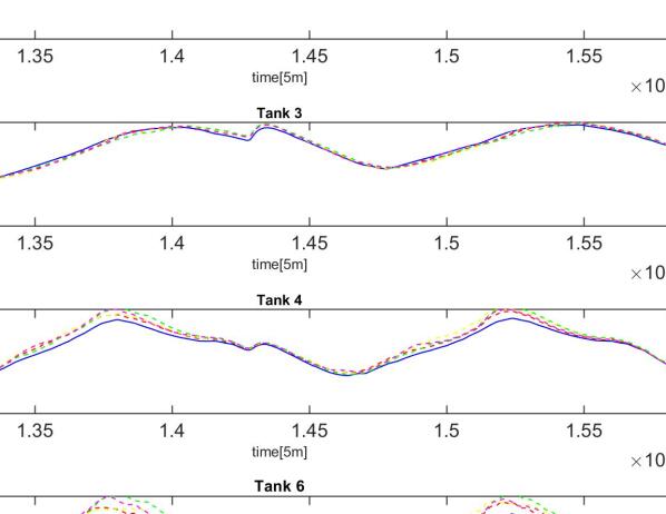
Figure 2: The volumes for the tanks with controllable orifices (Tank 2, Tank 3, Tank 4, Tank 6) for the CC-MPCs with probability confidence levels $\gamma$ of 100-60%.

4.2 CC-MPC with Various Uncertainty Bounds

The uncertainty bound describes the interval the uncertainty can take. For these simulations, a constant lower bound of zero is used; while the upper bound is defined as a percentage $p$ of the actual inflow above the expected rain inflow, see (51). The standard deviation of the uncertainty is assumed a third of the actual rain inflow times the percentage $p$, while the expectation is assumed equal to the actual rain. For normal distributions, this leads to the bound to be defined as

$$bound=[0,E\{q\}+p\mu]$$ (51)

corresponding to the 99.7% confidence interval of a corresponding unbounded distribution, if expectation matches the actual inflow. The CC-MPC is tested with percentage $p$ bounds of 25%, 50% and 75%. From Tables 5 and 6, we can observe the resulting CSO volume and WWTP volume, respectively. It can be observed that the deviations from the results of the deterministic MPC are negligible of up to a few hundred cubic meters. Figure 3 provides detailed dynamic evolution for the tank volumes of CC-MPC with uncertainty bounds of 25%, 50% and 75%, confirming conclusions obtained from Table 5 showing that the deviations brought by CC-MPCs are negligible. On another hand, it can be observed from Figure 3 that, the larger the uncertainty bound is, the smaller the tank volume is, which may cause less CSOs to the corresponding tank. This is because the larger uncertainty bounds make the CC-MPC generate more conservative orifice operations with the function of preventing CSOs. This conclusion is also in agreement with the basic deviations trends for the tanks CSO comparisons in Table 5.

Tank &	MPC	CC-MPC	CC-MPC	CC-MPC
Pipes		25%	50%	75%
T1	93251	93067	92927	92795
T2	15484	15543	15544	15544
T3	34017	34267	34313	34067
T4	4814	4814	4814	4814
T5	15147	15147	15147	15147
T6	37950	37939	37946	37673
P7	4016	4016	4015	4016
P8	16207	16203	16191	16207
P9	4030	4029	4029	4030
P10	4838	4839	4842	4838
River	183754	183879	183778	183412
Creek	45996	45984	45990	45718
Total	229750	229864	229768	229130
R. %		-0.0680%	-0.0131%	0.1861%
C. %		0.0261%	0.0130%	0.6044%
Tot. %		-0.0496%	-0.0078%	0.2699%

Table 5: Overflow results of the SWMM simulations with different controllers: MPC and CC-MPC with the uncertainty bound of 25-75%.

	MPC	CC-MPC	CC-MPC	CC-MPC
		25%	50%	75%
WWTP Vol.	3772057	3772086	3772159	3772676
Imp. %		0.0008%	0.0027%	0.0164%

Table 6: Treated Wastewater results of the SWMM simulations with different controllers: MPC, and CC-MPC with the uncertainty bound of 25-75%.

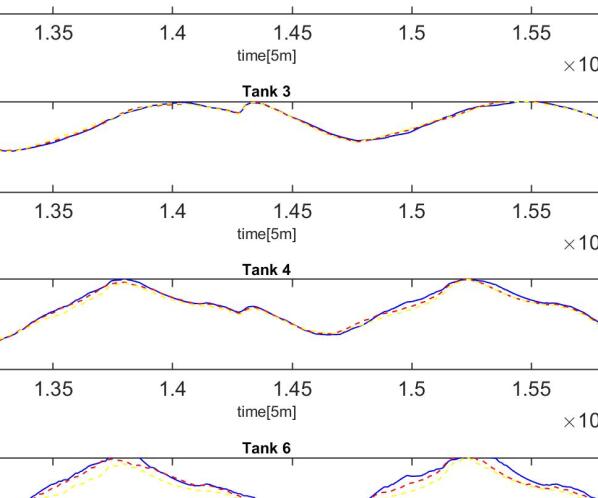
Figure 3: The volumes for the tanks with controllable orifices (Tank 2, Tank 3, Tank 4, Tank 6) for the CC-MPC with the uncertainty bound of 25-75%

4.3 CC-MPC with Various Scaled Biases

In this section, the percentage bound on the uncertainty are kept constant, 50%, instead the expected inflow is introduced as a scaled version of the actual rain inflow, given by

$$E\{q\}=aq^{actual}$$ (52)

Both the CC-MPC and the MPC are tested with 20% and 10% underestimated inflow, perfect forecast, and 10% and 20% overestimated inflow. The results can be seen in Table 7 and 8, for the CSO volume and the WWTP volume, respectively. We can observe that if the expected inflow is overestimated then both types of MPC perform relatively worse as the overestimation increases with respect to CSO volume, and slight improvement of WWTP volume. When the inflow is underestimated, then the MPC performs significantly worse than the MPC with perfect forecast, when regarding CSO but only slightly better for the WWTP volume. For the CC-MPC, both the total CSO and WWTP results are relatively close to the MPC with perfect forecast, but with the drawback of the distribution of the CSOs being significantly worse for the creek. Figure 4 gives detail volume comparisons for the controllable tanks under CC-MPC with different scaled bias through a two-day simulation (day 10 and day 11). The dynamics of Figure 4 confirm that CC-MPC with an underestimated inflow performs significantly worse than that the CC-MPC with overestimated inflows. The explanation for this conclusion is also due to less conservative generated by the underestimated inflows. Moreover, the larger scales tend to have more differences in terms of tank volumes.

Tank &	MPC	CC-MPC	MPC	CC-MPC	MPC	CC-MPC	MPC	CC-MPC	MPC	CC-MPC
Pipes	-20%	-20%	-10%	-10%	0%	0%	10%	10%	20%	20%
T1	96776	90004	95187	91355	93251	92927	94419	94728	96383	96615
T2	16727	16801	15957	16023	15484	15544	15384	15383	15317	15316
T3	33182	33298	33842	33857	34017	34313	34239	34065	33928	34304
T4	5938	5960	5191	5206	4814	4814	4730	4729	4714	4713
T5	15147	15147	15147	15147	15147	15147	15147	15147	15147	15147
T6	39252	39082	38341	38296	37950	37946	37790	37770	37908	37836
P7	4015	4015	4016	4015	4016	4015	4015	4016	4015	4015
P8	16195	16190	16208	16195	16207	16191	16188	16203	16188	16191
P9	4029	4029	4030	4029	4030	4029	4028	4029	4028	4029
P10	4841	4843	4837	4841	4838	4842	4843	4839	4843	4842
River	188805	182242	186369	182623	183754	183778	184949	185094	186519	187129
Creek	47297	47126	46387	46341	45996	45990	45834	45815	45952	45880
Total	236102	229368	232756	228964	229750	229768	230782	230909	232470	233008
R. %	-2.7488	0.8228	-1.4231	0.6155		-0.0131	-0.6503	-0.7292	-1.5047	-1.8367
C. %	-2.8285	-2.4567	-0.8501	-0.7501		0.0130	0.3522	0.3935	0.0957	0.2522
Tot. %	-2.7647	0.1663	-1.3084	0.3421		-0.0078	-0.4492	-0.5045	-1.1839	-1.4181

Table 7: Overflow results of the SWMM simulations with different controllers: MPC and CC-MPC under different scaled bias.

	MPC	CC-MPC	MPC	CC-MPC	MPC	CC-MPC	MPC	CC-MPC	MPC	CC-MPC
	-20%	-20%	-10%	-10%	0%	0%	10%	10%	20%	20%
WWTP Vol.	3765554	3772166	3769365	3772992	3772057	3772159	3771015	3770672	3769214	3768942
Imp. %	-0.1724	0.0029	-0.0714	0.0248		0.0027	-0.0276	-0.0367	-0.0754	-0.0826

Table 8: Treated Wastewater results of the SWMM simulations with different controllers: MPC, and CC-MPC under different scaled bias.

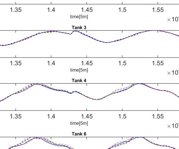
Figure 4: The volumes for the controllable tanks under CC-MPC with different scaled bias.

4.4 CC-MPC with Various with Offset Biases

In this section, the bias is changed from a scaling to an offset, see (53). Both the CC-MPC and the MPC are tested with zero offset and three positive offsets. The sizes of the offsets are the annual mean inflow (0.02) times the factors of 1 and 0.25, and 10 times the dry-weather inflow (0.1)

$$E\{q\}=q^{actual}+b$$ (53)

The results of both MPC types can be seen in Table 9 and 10 for the CSO and WWTP volume, respectively. We can observe that for both non-zero offsets, the CSO is significantly worse, with the offset of 0.1 being even worse. The results of the WWTP volume are also worse than the MPC with perfect forecast. Figure 5 gives more information about the performance of CC-MPC under different offsets. The differences in tank volume among CC-MPC using different offsets are compared. As always, the more volume in the tank indicates an increased chance of having more CSOs. From Figure 5, we can conclude that CC-MPC with 0.1 offset have more tank volume than that the offsets, which means, CC-MPC with 0.1 offset behaves worse than that of MPC. However, the CC-MPC with 0.005 and 0.02 did not show a clear trend.

Tank &	MPC	CC-MPC	MPC	CC-MPC	MPC	CC-MPC	MPC	CC-MPC
Pipes		0	0.005	0.005	0.02	0.02	0.1	0.1
T1	93251	92927	93655	93856	96472	96590	131407	130211
T2	15484	15544	15387	15450	15453	15452	15847	15511
T3	34017	34313	33975	34322	34086	34485	36811	36548
T4	4814	4814	4728	4728	4639	4644	4465	4465
T5	15147	15147	15147	15147	15147	15147	15147	15147
T6	37950	37946	37916	37961	37877	37780	37907	37763
P7	4016	4015	4015	4015	4015	4016	4016	4016
P8	16207	16191	16188	16193	16188	16203	16203	16203
P9	4030	4029	4028	4029	4028	4029	4029	4029
P10	4838	4842	4843	4842	4843	4839	4839	4839
River	183754	183778	183922	184536	186828	187360	224718	222925
Creek	45996	45990	45959	46005	45920	45825	45952	45808
Total	229750	229768	229881	230541	232748	233185	270670	268733
R. %		-0.0131	-0.0914	-0.4256	-1.6729	-1.9624	-22.2928	-21.3171
C. %		0.0130	0.0804	-0.0196	0.1652	0.3718	0.0957	0.4087
Tot. %		-0.0078	-0.0570	-0.3443	-1.3049	-1.4951	-17.8107	-16.9676

Table 9: Overflow results of the SWMM simulations with different controllers: MPC and CC-MPC under different off-set biases.

	MPC	CC-MPC	MPC	CC-MPC	MPC	CC-MPC	MPC	CC-MPC
		0	0.005	0.005	0.02	0.02	0.1	0.1
WWTP Vol.	3772057	3772159	3771978	3771575	3768823	3768643	3731689	3733651
Imp. %		0.0027	-0.0021	0.0001	-0.0857	-0.0905	-1.0702	-1.0182

Table 10: Treated Wastewater results of the SWMM simulations with different controllers: MPC, and CC-MPC under different off-set biases.

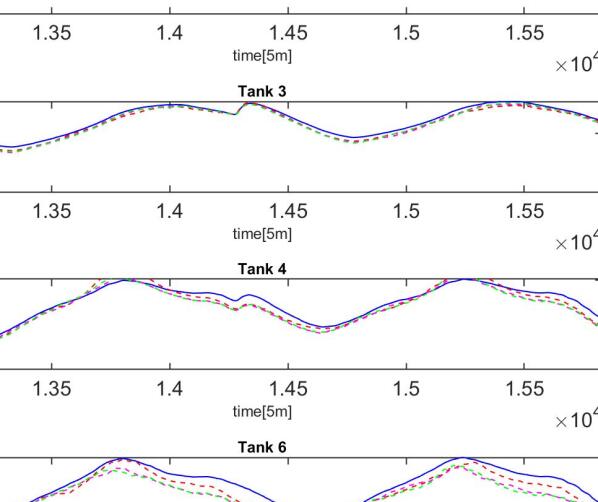
Figure 5: The volumes for the controllable tanks under CC-MPC using different offsets.

From the above results, we can infer that the CC-MPC is capable of handling different type of uncertainties, and for those type of uncertainties, it performs similarly to the deterministic MPC. We can further see that the CC-MPC, while not performing that well with constant offset biases, these biases were also outside the uncertainty bound, practically making the CC-MPC as blind as the deterministic MPC. In real-world scenarios, the uncertainty of the inflow is not exactly as the one used here. Instead the uncertainty bound would vary across the prediction horizon, as would do the biases of the expected inflow.

5 Conclusion

A stochastic MPC has been applied to a hydrodynamic SWMM model of the Astlingen urban drainage benchmark network, using a chance-constraint formulation of MPC. A comparison study of the application of both CC-MPC and MPC has been done for several scenarios and types of uncertainties in forecasts, involving both biases in the forecast to different sizes of the uncertainty. Based on the simulations, we can conclude that only the uncertainty regarding biases has an effect on the performance of CC-MPC. Furthermore, it could be observed that the performance of both type of MPC considered deteriorate similarly with respect to CSO volume, when the forecast overestimates the rain inflow. However, when the forecast underestimates the rain inflow, then the CC-MPC performs similarly to the ideal case, while the performances of deterministic MPC deteriorates.

References

- [1] J. M. Maciejowski, Predictive Control: with constraints, Pearson, 2002.
- [2] R. Halvgaard, A. K. V. Falk, Water system overflow modeling for model predictive control, in: Proceedings of the 12th IWA Specialised Conference on Instrumentation, Control and Automation, Proceedings of the 12th IWA Specialised Conference on Instrumentation, Control and Automation, 2017.
- [3] J. L. Svensen, H. H. Niemann, N. K. Poulsen, Model predictive control of overflow in sewer networks: A comparison of two methods, in: Proc. of the 4th Int. Conf. on Control and Fault-Toleran Systems, Proc. of the 4th Int. Conf. on Control and Fault-Toleran Systems, 2019, pp. 412–417.
- [4] C. Sun, J. L. Svensen, M. Borup, V. Puig, G. Cembrano, L. Vezzaro, An mpc enabled swmm implementation of the astlingen rtc benchmaking network, Water 12 (1034) (2020).
- [5] M. S. Gelormino, N. L. Ricker, Model predictive control of a combined sewer system, INT. J. CONTROL 59 (3) (1994) 793–816.
- [6] C. Sun, B. Joseph, T. Maruejouls, G. Cembrano, E. Muñoz, J. Meseguer, A. Montserrat, S. Sampe, V. Puig, X. Litrico, Efficient integrated model predictive control of urban drainage systems using simplified conceptual quality models, 14th IWA/IAHR International Conference on Urban Drainage, Prague, 2017, pp. 1848–1855.
- [7] C. Sun, B. Joseph, G. Cembrano, V. Puig, J. Meseguer, Advanced integrated real-time control of combined urban drainage systems using mpc: Badalona case study, 13th International Conference on Hydroinformatic, Palermo, 2018, pp. 2033–2041.
- [8] C. Ocampo-Martinez, Model Predictive Control of Wastewater Systems, Advances in Industrial Control, Springer, 2010.
- [9] M. Marinaki, M. Papageorgiou, Optimal Real-time Control of Sewer Networks, Advances in Industrial Control, Springer, 2005.
- [10] L. Cen, Y. Xi, Aggregation-based model predictive control of urban combined sewer networks, in: Proc. of the 7th Asian Control Conference, Proc. of the 7th Asian Control Conference, 2009.
- [11] C. Sun, G. Cembrano, V. Puig, J. Meseguer, Cyber-physical systems for real-time management in the urban water cycle, in: Proceedings of the 4th International Workshop on Cyber-Physical Systems for Smart Water Networks, 2018, pp. 3–5.
- [12] C. Sun, B. Joseph-Duran, T. Maruejouls, G. Cembrano, J. Meseguer, V. Puig, X. Litrico, Real-time control-oriented quality modelling in combined urban drainage networks, in: Proceedings of the IFAC 2017 World Congress, 2017, pp. 4002–4007.
- [13] C. Sun, V. Puig, G. Cembrano, Real-time control of urban water cycle under cyber-physical systems framework, Water 12 (406) (2020).
- [14] B. Joseph-Duran, J. Meseguer, G. Cembrano, T. Maruejouls, Closed-loop simulation of real-time controllers for urban drainage systems using high resolution hydraulic simulators, in: Proceedings of the 14th IWA/IAHR International Conference on Urban Drainage, 2017.
- [15] G. Cembrano, J. Quevedo, M. Salamero, V. Puig, J. Figueras, J. Marti, Optimal control of urban drainage systems. acase study, Control Engineering Practice 12 (2004) 1–9.
- [16] P. Overloop, Model Predictive Control on Open Water Systems, Delft University Press: Delft, 2006.
- [17] J. L. Svensen, H. H. Niemann, A. K. V. Falk, N. K. Poulsen, Chance-constrained model predictive control - a reformulated approach suitable for sewer networks, Advanced Control of Applications, Submitted.
- [18] J. M. Grosso, C. Ocampo-Martinez, V. Puig, B. Joseph-Duran, Chance-constrained model predictive control for drinking waternetworks, Journal of Process Control 24 (2014) 504–516.
- [19] H. Arellano-Garcia, G. Wozny, Chance constrained water quality management model for reservoir systems: I. strict monotonicity, Comput. Chem. Eng. 33 (10) (2009) 1568–1583.
- [20] A. Dhar, B. Datta, Chance constrained water quality management model for reservoir systems, ISH J. Hydraul. Eng. 12 (3) (2006) 39–48.
- [21] M. Evans, M. Cannon, B. Kouvaritakis, Linear stochastic mpc under finitely supported multiplicative uncertainty, Proc. of the 2012 American Control Conference, 2012.
- [22] S. Garatti, M. C. Campi, S. Garatti, M. Prandini, The scenario approach for systems and control design, Annual Reviews in Control 33 (2009) 149–157.
- [23] A. Mesbah, Stochastic model predictive control: An overview and perspectives for future research, IEEE Control Systems Magazine (2016) 30–44doi:10.1109/MCS.2016.2602087.
- [24] B. Kouvaritakis, M. Cannon, Model Predictive Control - Classical, Robust and Stochastic, Advances Textbooks in Control and Signal Processing, Springer, 2016. doi:10.1007/978-3-319-24853-0.
- [25] Z. Wan, M. V. Kothare, Robust output feedback model predictive control using off-line linear matrix inequalities, Journal of Process Control 12 (7) (2002) 763–774.
- [26] L. Magni, G. D. Nicolao, R. Scattolini, F. Allgöwer, Robust model predictive control for nonlinear discrete-time systems, International Journal of Robust and Nonlinear Control 13 (3-4) (2003) 229–246.
- [27] Z. Q. Sun, L. Dai, K. Liu, Y. Q. Xia, K. H. Johansson, Robust mpc for tracking constrained unicycle robots with additive disturbances, Automatica 90 (2018) 172–184.
- [28] M. Schütze, M. Lange, M. Pabst, U. Haas, Astlingen - a benchmark for real time control (rtc), Water Sci & Technol 2017 (2) (2018) 552–560.
- [29] V. P. Singh, Hydrologic Systems. Volume 1: Rainfall-runoff modelling, Prentice Hall, 1988.
- [30] P. Karantonis, C. Weber, Use of iso measurement uncertainty guidelines to determine uncertainties in noise & vibration predictions and design risks, in: Proceedings of ACOUSTICS, Proceedings of ACOUSTICS, Brisbane, Australia, 2016, pp. 1–9.
-
[31]
P. Scott, UNCERTAINTY
IN MEASUREMENT: NOISE AND HOW TO DEAL WITH IT, 2003.
URL http://physics.ucsc.edu/{$∼$}drip/133/ch2.pdf