Crack Localization and the Interplay between Stress Enhancement and Thermal Noise

Abstract

We study the competition between thermal fluctuations and stress enhancement in the failure process of a disordered system by using a local load sharing fiber bundle model. The thermal noise is introduced by defining a failure probability that constitutes the temperature and elastic energy of the fibers. We observe that at a finite temperature and low disorder strength, the failure process, which nucleate in the absence of any thermal fluctuation, becomes spatially uncorrelated when the applied stress is sufficiently low. The dynamics of the model in this limit lies closely to the universality class of ordinary percolation. When applied stress is increased beyond a threshold value, localized fractures appear in the system that grow with time. We identify the boundary between the localized and random failure process in the space of temperature and applied stress, and find that the threshold of stress corresponding to the onset of localized crack growth increases with the increase of temperature.

1 Introduction

Growth of fractures under external stress in heterogeneous materials, such as concrete or fiber-reinforced composites, depends on the interplay between material disorder and local stress concentration throughout the failure process. The heterogenities compete with the local stress enhancement preventing the growth of a single unstable crack until the stress exceeds a critical value, beyond which it undergoes a catastrophic failure [1]. In addition to material heterogeneities, there is also the disorder induced by thermal fluctuations. These combined with an applied stress or strain can cause failure with time even if the applied stress is below the critical value [2]. This phenomenon is known as creep failure. The study of creep failure is an essential but notoriously difficult subject that has important engineering applications. Of special importance is the statistics connected to the time elapsed until creep failure occurs, the creep lifetime [3, 4].

The underlying physical mechanisms behind creep are the accumulation of plastic strain and damage in the system. In order to model the creep failure in disordered systems, mechanisms for such aging processes are needed to be taken into account in addition to the structural heterogeneities. However, the fracture of heterogeneous solids is yet hard to handle with the elasticity theory and therefore there have been some alternative approaches. The Voight model [5] for precursory strain has been explored by Main [6] in order to understand the sub-critical crack growth dynamics. The model can reproduce the time-dependent strain rate observed in experiments [7]. On the other hand, time-dependent failure has been investigated widely [8, 9, 10, 11, 12, 13, 14, 15, 16, 17, 18] using a simple and intuitive model for disordered solids, known as the fiber bundle model [19, 20, 21, 22, 23, 24, 25]. Here, the thermal fluctuations are incorporated in terms of noise or probabilistic time evolution in order to include the effect of temperature during failure. These studies in fiber bundle model appear to be successful in explaining the time-dependent strain rate as well as the temperature and the stress (or strain) dependencies in the creep lifetime [8, 9, 10, 11]. Hidalgo et al., however, obtained somewhat different results [14, 15] for the temperature and stress dependence of creep lifetime from those in the above-mentioned stochastic models [8, 9, 10, 11] by introducing a time evolution equation for the strain of each constituent (i.e., fiber) based on the Kelvin-Voigt rheology. Danku and Kun consider a damage accumulation process in each fiber by introducing a damage variable and the time evolution equation [17]. Interestingly, fiber bundle model at its simplest form can exhibit creep-like behaviors even in the absence of any thermal fluctuations, damage variables, or rheological constitutive laws [26, 27]. In particular, Roy and Hatano assumed the time evolution in a simple fiber bundle model and derived the time-dependent strain rate [27].

Here we study the role of thermal fluctuations in the failure process of a disordered system by using a local-load sharing (LLS) fiber bundle model where the material disorder and local stress enhancements compete. We introduce thermal noise in the model by a probabilistic algorithm that is based on the elastic energy and the breaking energy of a fiber. This creates time-dependent fluctuations in the model in addition to the quenched system disorder. The interplay between these two types of disorders and the local stress enhancements creates non-trivial dynamics in the failure process. More specifically, we show that the introduction of thermal noise makes the failure process non-localized even at low system disorder under low stress, which otherwise would be localized in the absence of thermal fluctuations. We characterize the non-localized growth regime by measuring the geometrical properties of the cracks and we show that they belong to the percolation universality class. We also identify the boundary between the localized and non-localized regimes in the temperature-applied stress plane. We present the model in Section 2 and the numerical results in Section 3 where we also discuss the results. We conclude in Section 4.

2 Model description

The fiber bundle model consists of $N$ Hookean springs or fibers placed between two clamps under an external force $F$ carried by the fibers. The extension $x_{i}$ of a fiber $i$ under a force $f_{i}$ follows the relation $f_{i}=\kappa x_{i}$. All the fibers have the same elastic constant $\kappa$. Each fiber is assigned a maximum extension $\epsilon_{i}$. If this value is exceeded, that particular fiber fails. The distribution of the thresholds $\epsilon_{i}$ among the fibers models the heterogeneity of the material. When a fiber fails, the load it was carrying is distributed among the surviving fibers according to a load-sharing scheme that models the way the forces are distributed among the surviving fibers. If the load carried by the failed fibers is distributed uniformly over all the surviving fibers, we have the Equal Load Sharing (ELS) scheme. With this scheme, there is no local stress enhancement in the model. On the other hand, if the load carried by the failing fiber is distributed evenly among the fibers bordering the cluster of broken fibers to which the failed fiber belong, we are dealing with the Local Load Sharing (LLS) scheme. Here local stress enhancement competes with the local heterogeneity. The ELS fiber bundle model was initially introduced by Peirce [19] to model the strength of yarn and since Daniels’ paper [20], the model caught on in the mechanics community. Sornette introduced the ELS fiber bundle model to the statistical physics community in 1992 [28] which lead the community to explore the rich avalanche statistics [29, 30, 31, 32] and analytical tractability of the ELS model. The local load-sharing (LLS) fiber bundle model was introduced by Harlow and Phoenix [33, 34] as a one-dimensional array of fibers. There are also intermediate models between ELS and LLS models, e.g. the model by Hidalgo et al. [12], where the load of the failing fiber is distributed according to a power law in the distance from the failed fiber. Another is the soft clamp model [35, 36, 37, 38], where the infinitely stiff clamps are replaced by clamps with finite elastic constant causing the load of the failing fiber for be distributed among the surviving in accordance with the elastic response of the soft clamps.

Here we consider an LLS fiber bundle model that is based on a history independent redistribution scheme [39] so that the complete stress field at any instance can be calculated from the present arrangement of intact and broken fibers without knowing any information about order in which the fibers failed. For this, we define a crack, which is a cluster of $s$ failed fibers defined as in percolation theory [40, 41]. The perimeter of the crack is the set of $h$ intact fibers that are nearest neighbors to the failed fibers in that crack. These nearest neighbors define the hull of the cluster [42]. The force on an intact fiber $i$ at any instance is then calculated by

$$f_{i}=f\left(1+\sum_{J(i)}\frac{s_{J(i)}}{h_{J(i)}}\right)\;,$$ (1)

where $f=F/N$, the force per fiber. The summation runs over all cracks $J(i)$ that are neighbors to fiber $i$.

Here we study the fiber bundle at a temperature $T$ subjected to a constant external stress $F$ that is less than the critical breaking stress for the bundle. In order to do this, we introduce changes to the LLS model. Due to thermal noise, a fiber $i$ may fail even if the force on it fulfills $f_{i}<\kappa\epsilon_{i}$. The elastic energy of a fiber at extension $x_{i}$ is $\kappa x_{i}^{2}/2$ and the elastic energy at failure is $\kappa\epsilon_{i}^{2}/2$. This energy is dissipated, i.e., lost as elastic energy at failure. We introduce a discrete time variable $t$ to be defined below. We define a failure probability

$$P_{i}(t,T)=\exp\left[{-\frac{\kappa(\epsilon_{i}^{2}-f_{i}^{2})}{2k_{B}T}}\right]\;,$$ (2)

where $k_{B}$ is the Boltzmann constant. In the following we set $\kappa/k_{B}=1$ for simplicity. The simulation starts at $t=0$ with all fibers intact and each carrying a finite load $f_{i}=f$. The failure probability $P_{i}$ is then calculated for each fiber $i$. We then generate a random number $r_{i}$ uniformly distributed between $0$ and $1$ for each fiber $i$, which we compare to $P_{i}$. All the fibers for which $r_{i}<P_{i}$ fails. The forces are then redistributed according to Eq. 1 and time $t$ is increased by 1. This procedure is repeated until all fibers have failed. Note that the failure probability $P_{i}$ is an increasing function of the temperature $T$ as well as of the local stress $f_{i}$ which also increases with time due to the failures. When $f_{i}>\epsilon_{i}$, $P_{i}$ is always greater than one for any temperature $T$ and the fiber always breaks. Furthermore, as the temperature is changed towards zero ($T\to 0$), the failure probability $P_{i}$ is approached towards a step function from $0$ to $1$ at $f_{i}=\epsilon_{i}$. This means, at $T=0$, there is no contribution from the thermal noise to the breaking probability and a fiber only breaks due to the local stress. This leads the model to approach the conventional LLS model at $T=0$ [43]. With increasing temperature, values of $P_{i}$ increases throughout the range of $f_{i}$ and becomes less dependent on how $f_{i}$ is close to the threshold $\epsilon_{i}$. Recently, a similar probabilistic failure process was adopted to explore the creep failure in ELS fiber bundle model [44].

For the disorder in the failure thresholds $\epsilon_{i}$, we consider a distribution that has only one control parameter. The thresholds in this distribution are generated by calling a random number ($r_{i}$) over the unit interval and raising it to a power $D$, therefore $\epsilon_{i}=r_{i}^{D}$. This corresponds to the cumulative distribution [45, 46],

$$P(\epsilon)=\begin{cases}\epsilon^{1/|D|}\;,\epsilon\in[0,1]&\text{when}\;D>0\;,\\ 1-\epsilon^{-1/|D|}\;,\epsilon\in[1,\infty)&\text{when}\;D<0\;.\end{cases}$$ (3)

The strength of disorder in this distribution is controlled by the value of $|D|$. Moreover, $D>0$ and $D<0$ respectively correspond to the distributions with power law tails towards weaker and stronger fibers. The interplay between such disorder and local stress enhancement in LLS fiber bundle model in the absence of any thermal noise was explored recently [43]. There, phase transitions from a localized fracture regime to random fractures were observed while increasing the disorder. Interestingly, the transition for $D<0$ was of first order and for $D>0$ was of second order. In the present work, we investigate the effect of thermal noise on the failure dynamics and study its effect on crack localization, and we limit our simulations in the low disorder limit at $D=0.02$, where the failure was localized in the absence of temperature. However, as we will see in the next section that the presence of temperature makes the fracture growth of this regime non-localized when the stress is low. We present our numerical results in the following.

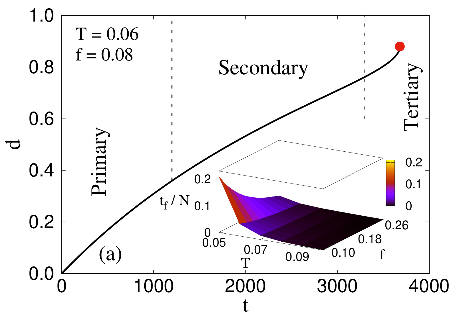
Figure 1: The variation of damage $d$ with time $t$ for $T=0.06$ and $f=0.08$ showing three regimes of creep like failure, a primary regime a secondary regime and a tertiary regime. The red dot shows the final failure point. The $x$-coordinate of the point corresponds to the failure time $t_{\rm f}$. The inset of the figure shows how $t_{\rm f}$ decreases with the increase of temperature and applied stress.

3 Results

We consider a bundle of $N=256\times 256$ fibers in two dimensions (2D) with periodic boundary conditions. The results are averaged over $1000$ realizations of samples. Simulations are performed for different values of temperature ($T$) and external stress ($f=F/N$) which are kept constant throughout a simulation. The thermal noise initiates a creep failure process to break the system over time even if the applied stress is less than the critical value. Depending on the thermal noise and local stress enhancements, many or few fibers may fail simultaneously. The growth of damage in this process is illustrated in Fig. 1 where we plot the damage $d$ — defined as the number of failed fibers divided by $N$ — as a function of $t$ for a stress $f=0.08$, which is lower than the critical stress. The plot shows three regimes of failure process, a primary regime where the rate of damage decreases with time, a secondary regime where the damage rate is almost constant, and a tertiary regime where the damage increases rapidly until the whole bundle fails. This is a qualitative characteristics that is generally observed during a creep failure [24]. The red dot at the end of the curve indicates the failure time $t_{\rm f}$ which depends on the temperature as well as on the applied stress. This is shown in the inset, where $t_{\rm f}$ decreases with increase of both $T$ and $f$, as a higher stress or temperature generates higher probability of failure at each time step, making the model go faster towards the global failure.

3.1 Localized vs non-localized fracture growth

The growth of cracks with time in the presence of temperature at two different external stress $f=0.1$ and $f=0.4$ are shown in Fig. 2. The intact clusters are colored by black and the individual clusters of failed fibers are marked with different colors. The pictures show two distinct regimes of crack growth. At low applied stress the subsequent failure events appear randomly in space, similar to the growth of percolation clusters. The clusters merge with time and a spanning cluster appears in the system similar to a percolating cluster that contains clusters of intact fibers of different sizes inside it. On the other hand, at high stress, localized clusters of failed fibers appear and that eventually merge. The localized clusters in this case are compact.

 

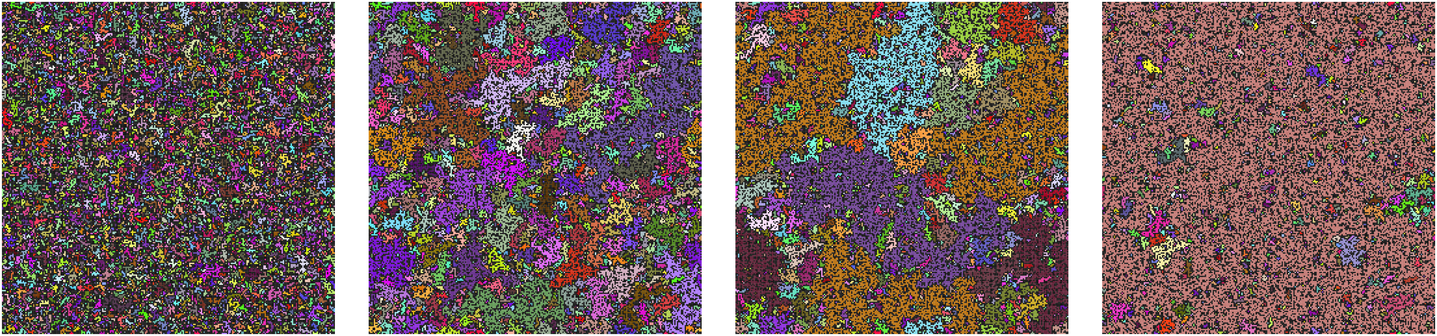
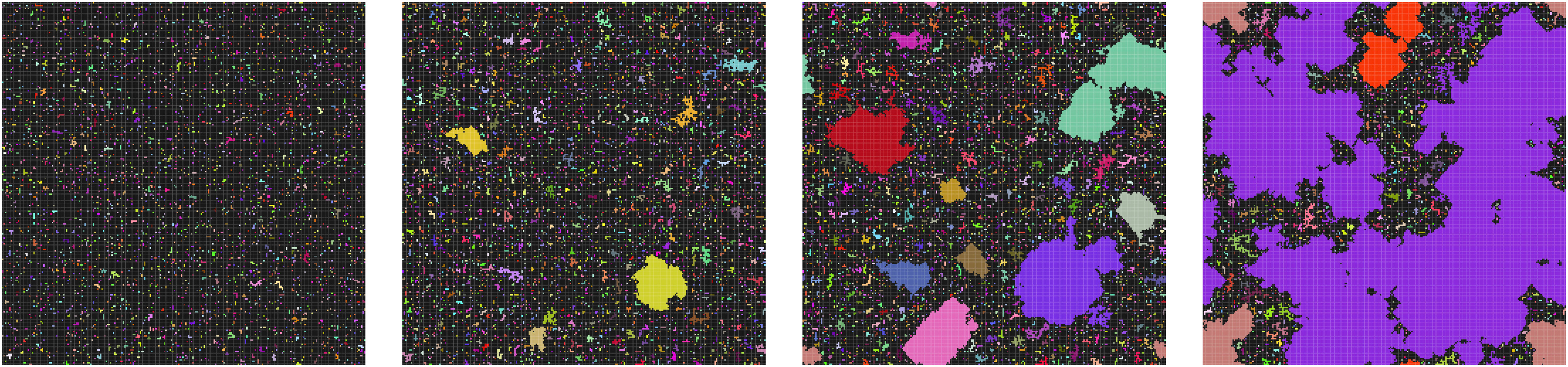
(a) (b)

Figure 2: Growth of cracks for two different applied stresses (a) $f=0.1$ and (b) $f=0.4$ in a bundle of $256\times 256$ fibers at temperature $T=0.06$. The thresholds are generated according to Eq. 3 at low disorder $D=0.02$. The snapshots correspond to $t=0.40t_{\rm f}$, $0.60t_{\rm{}_{f}}$, $0.64t_{\rm f}$ and $0.68t_{\rm f}$ for $f=0.1$, and $t=0.48t_{\rm f}$, $0.70t_{\rm{}_{f}}$, $0.79t_{\rm f}$ and $0.87t_{\rm f}$ for $f=0.4$. The intact fibers are colored by black and the other colors represent different clusters of broken fibers. At low applied stress, cracks appear randomly in the system whereas at high applied stress localized cracks are observed to grow within the system.

To study how the applied stress and temperature alter the failure dynamics from random fractures to localized crack growth, we measure three different geometrical quantities, the number density of clusters, the largest cluster size and the largest perimeter size as a function of damage $d$ for different values of $T$ and $f$. They are plotted in Fig. 3 (a), (b) and (c) respectively. In 3 (a), we plot the cluster number density $\rho$ as a function of $d$ for different applied stress ($f$) at temperature $T=0.06$. Here $\rho$ is defined as the number of clusters of failed fibers divided by the total number of fibers $N$, which shows a non-monotonic behavior with $d$. We observe $\rho=0$ at $d=0$ and $\rho=1$ as $d\to 1$, because all the fibers are then broken creating a single crack. In between, $\rho$ reaches a maximum value where the system contains maximum number of clusters. This maximum decreases with increasing $f$, and interestingly, the dependence of $\rho$ on $d$ shows a characteristic difference beyond an applied stress $f>f_{c}$ indicating a difference in the failure dynamics. These two different characteristics are highlighted in the inset for $f=0.20$ and $0.32$.

Next we measure the largest cluster size ($s_{\rm max}$) and the largest perimeter size ($h_{\rm max}$) as a function of $d$. In Fig. 3 (b) and (c), we plot $s_{\rm max}$ and $h_{\rm max}$ respectively, scaled by the number of fibers $N$. As we vary the applied stress $f$, both the quantities show a characteristic difference in the behavior below and above $f_{c}$. In the beginning of the process, small fractures appear in the system leading to small values of $s_{\rm max}$, which will eventually grow and merge with each other. For $f>f_{c}$, the increase in $s_{\rm max}$ starts at a much earlier point than that of $f<f_{c}$. This reflects the appearance of compact localized cracks early in the system for $f>f_{c}$, which grow more uniformly with time. Whereas for $f<f_{c}$, spatially uncorrelated failures occur at random in space preventing the appearance of a large cluster for a longer duration. At some point of time, these small clusters start to coalesce causing a sharp increase in $s_{\rm max}$ as seen in the figure. When the coalescence is over after creating a large crack in the system, $s_{\rm max}$ grows in a linear manner. Behavior of $s_{\rm max}$ shows similarity with that of percolation model for $f<f_{c}$ whereas above $f_{c}$ it deviates from such characteristic shape indicating the initiation of localization. These two behaviors for $f<f_{c}$ and $f>f_{c}$ are highlighted in the inset. The behavior of $h_{\rm max}$ shows a more interesting picture. It shows two different behavior for $f<f_{c}$ and $f>f_{c}$, however, the values of $h_{\rm max}$ are much smaller for $f>f_{c}$, that is in the localized regime. This indicates fractal type perimeter structure for $f<f_{c}$ compared to the perimeters of the localized cracks for $f>f_{c}$. Later in section 3.3, we will use $h_{\rm max}$ to calculate the values of $f_{c}$ and will show how the boundary between the non-localized and localized fracture regimes vary with the temperature $T$. For $f<f_{c}$, both $s_{\rm max}$ and $h_{\rm max}$ indicate percolation type dynamics during the failure process which we will explore in detail in the following.

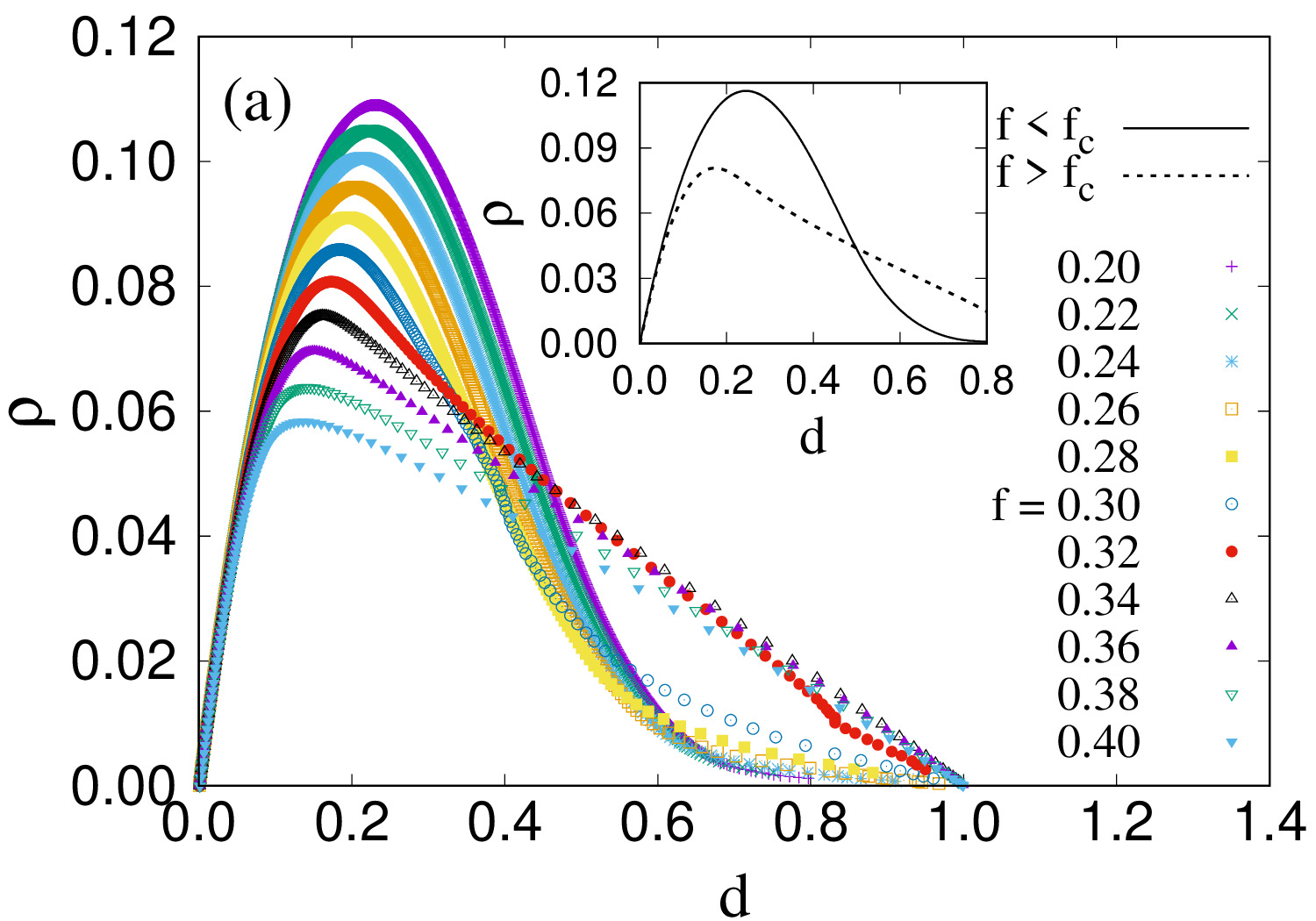
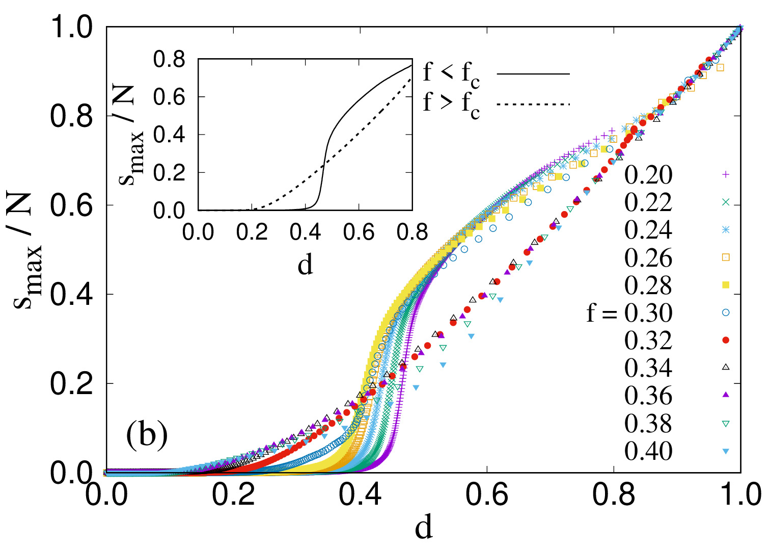
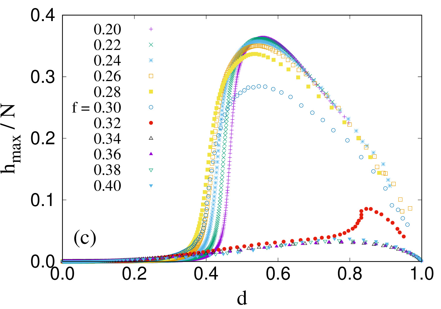
Figure 3: (a) Variation of cluster density $\rho$ with damage $d$ for $T=0.06$ while varying the applied stress $f$. Two distinct behaviors are observed for the non-localized and localized regimes corresponding to $f<f_{c}$ and $f>f_{c}$ respectively where $f_{c}=0.30$. These two behaviors are highlighted in the inset for $f=0.20$ and $0.32$. (b) Variation of the maximum crack size $s_{\rm max}$ normalized by the system size $N$, with damage $d$. The inset highlights the two different behaviors below and above $f_{c}$. (c) Variation of the normalized maximum hull size $h_{\rm max}/N$ with damage $d$. Notice that, the maxima of $h_{\rm max}$ for non-localized regime have much higher values compared to the localized regime indicating fractal structure of the clusters at $f<f_{c}$.

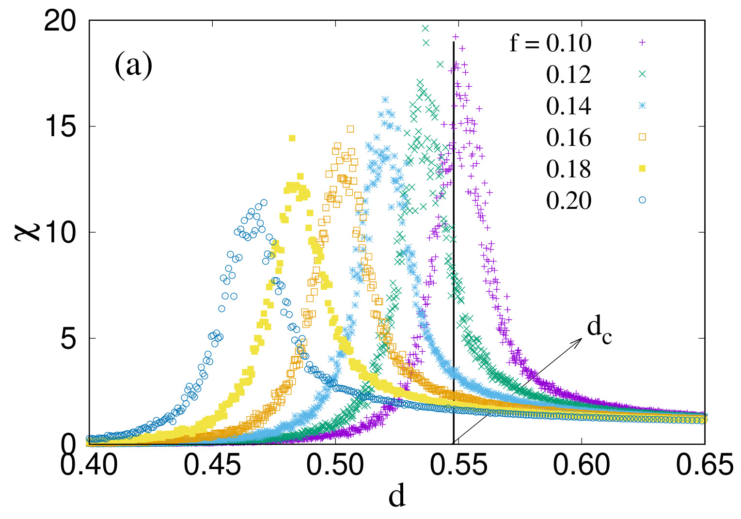
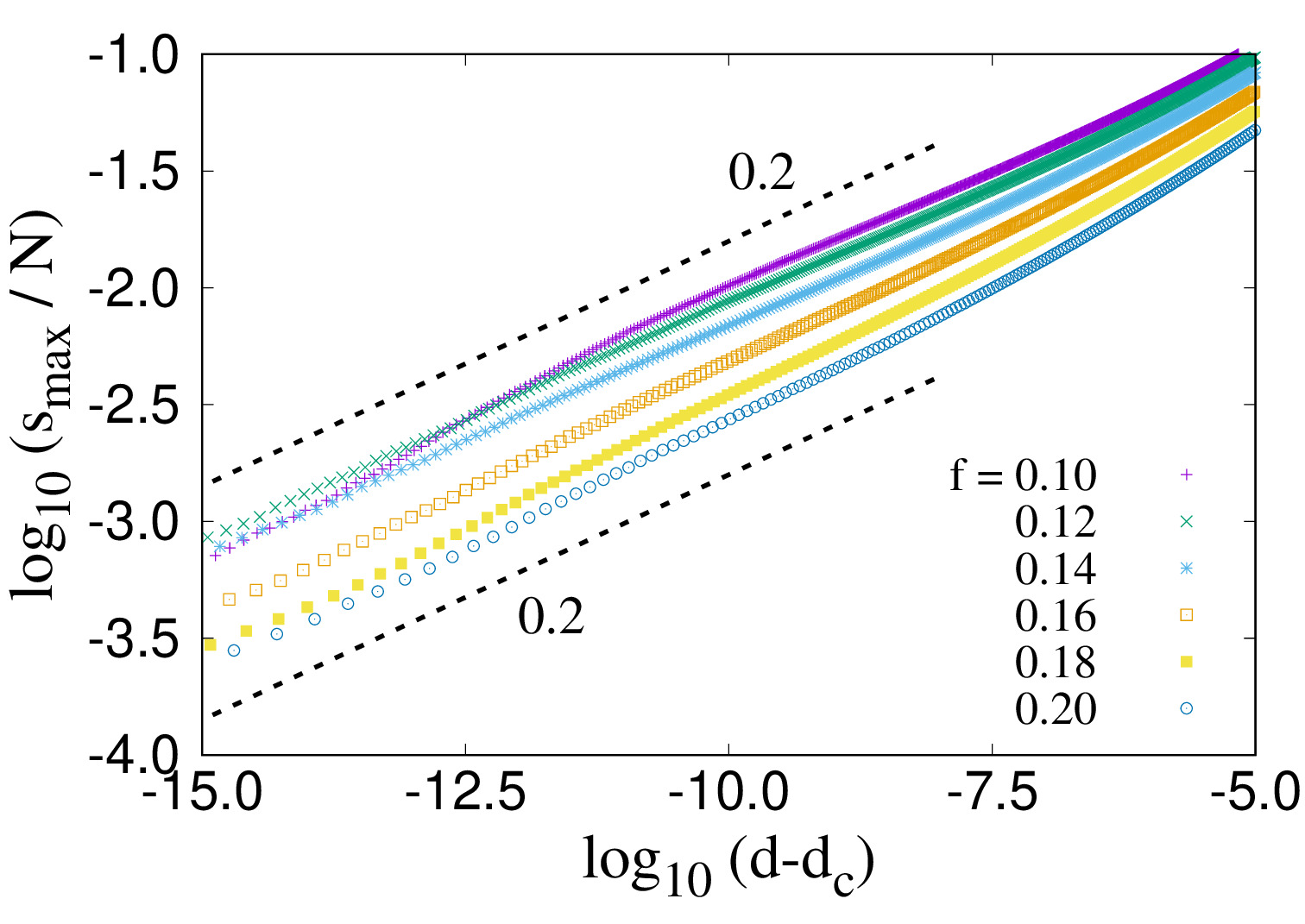
Figure 4: (a) The response function $\chi$, i.e., the rate of change of largest cluster size $s_{\rm max}$ as a function of the damage $d$. This is obtained by taking the derivative of $s_{\max}$ with respect of $d$ using the central difference technique. From the peaks, we find the values of critical damage $d_{c}$. In (b), we plot $s_{\rm max}/N$ with $(d-d_{c})$ where the slopes correspond to the exponent $\beta$ defined in Eq. 4. We observe $\beta$ around $0.2$, which however fluctuates with the applied stress. The full list of the values of $\beta$ for different applied stress will be given in Tab. 1.

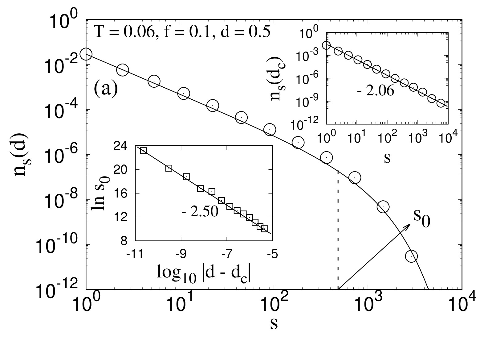
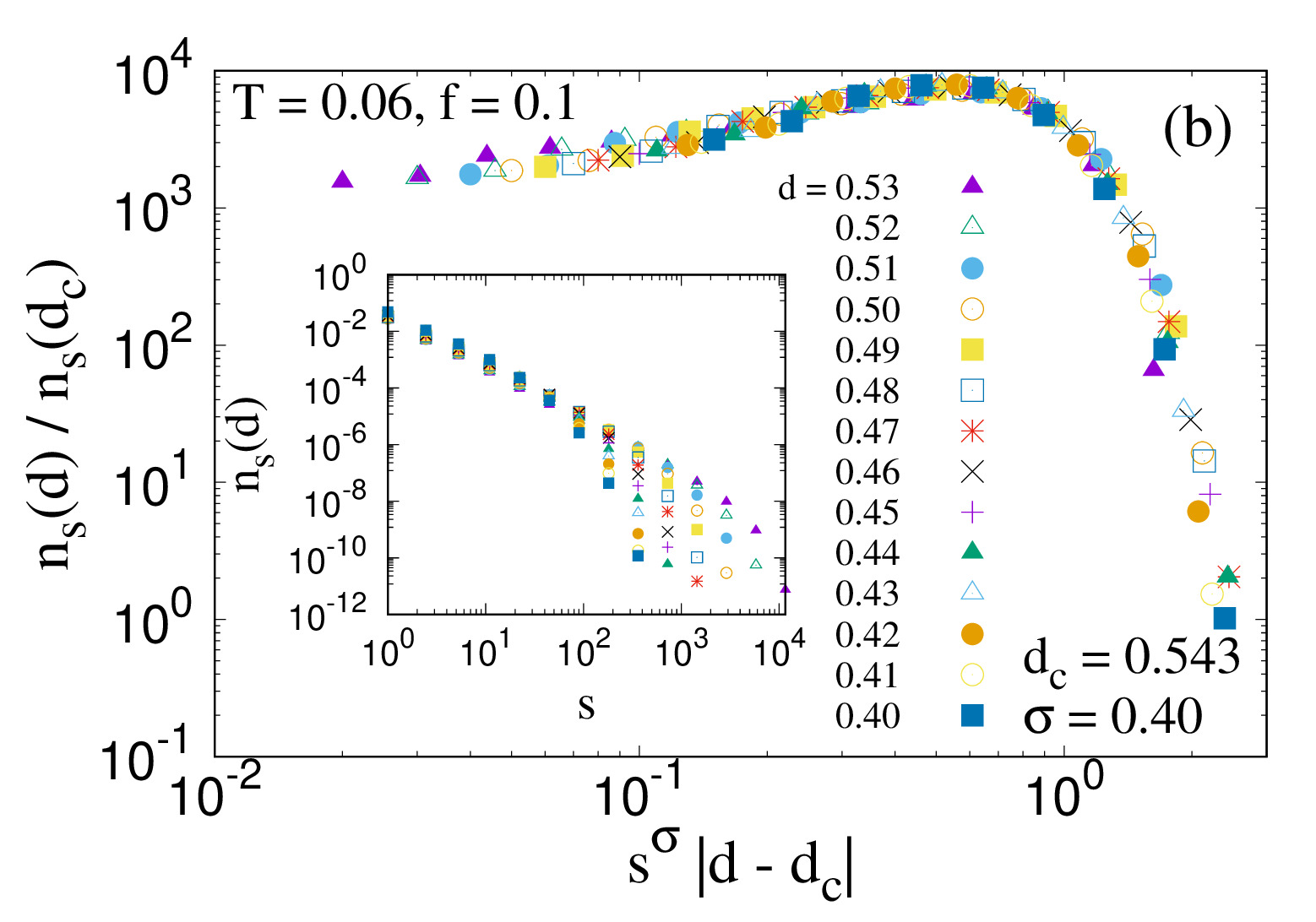
Figure 5: (a) Plot of cluster size distribution $n_{s}(d)$ at $d=0.5$ for $T=0.06$ and $f=0.10$. The circles represent simulation data and the solid line represents least square fitting of data with Eq. 8, where $\tau$ is $2.06$. The value of $\tau$ is obtained from the distribution $n_{s}(d_{c})$ using Eq. 6 as shown in the upper inset of (a). We obtain the values of $s_{0}$ from the least-square fitting for different values of $d$. The variation of $s_{0}$ with $|d-d_{c}|$ is shown the inset, the slope of which corresponds to $1/\sigma$ (Eq. 9). In (b), we plot the scaled cluster size distribution $n_{s}(d)/n_{s}(d_{c})$ as a function of the scaled variable $s^{\sigma}|d-d_{c}|$ for $T=0.06$ and $f=0.10$ where we have used $\sigma=1/2.50=0.40$ obtained from the previous plot. Here $d_{c}$ is $0.543$. In the inset, we show the unscaled behavior of $n_{s}(d)$ vs $s$ for different values of $d$.

3.2 Characterization of non-localized cluster growth for $f<f_{c}$

To characterize the growth of fractures in the non-localized regime we will now study the clusters geometries by using the percolation framework [40, 41]. We performed simulations at $T=0.06$ at different values of $f<f_{c}$. We found $f_{c}\approx 0.3$ for $T=0.06$ and therefore considered $f=0.10$, $0.12$, $0.14$, $0.16$ and $0.18$ for these simulations. To find a percolation threshold or a critical damage $d_{c}$, one can calculate the order parameter $P_{\infty}$ defined as the probability that a site belongs to an infinite cluster. $P_{\infty}$ can be measured from the number of sites ($s_{\rm max}$) that belong to the largest cluster and then by estimating $P_{\infty}=\lim_{N\to\infty}P_{N}$ where $P_{N}=s_{\rm max}/N$ averaged over all configurations. Ideally, $P_{\infty}$ approaches to $0$ from $1$ continuously as $d\to d_{c}$ from above. In our case, we have a finite system of $256^{2}$ fibers and therefore $P_{N}=s_{\max}/N$ does not meet to $0$ sharply at a particular value of $d$ (Fig. 3 (b)). We therefore measure the percolation threshold $d_{c}$ from the maximum of the response function $\chi$ of $P_{N}$, that is when the rate of change of $s_{\rm max}$ with $d$ is maximum. This is plotted in Fig. 4 (a) where the peaks of the plots determine the values of $d_{c}$ for different $f$. As $d\to d_{c}$ from above, $P_{\infty}$ approaches to zero with a critical exponent $\beta$ defined as,

$$P_{\infty}\sim(d-d_{c})^{\beta}\;.$$ (4)

In Fig. 4, we plot $s_{\rm max}/N$ as a function of $(d-d_{c})$ for different values of $f$ and from the slopes we find $\beta$ in the range of $0.18$ to $0.23$ with error bars ranging between $0.04$ to $0.07$ (see Tab. 1). For site percolation, $\beta=5/36$.

Next, we study the distribution of clusters of failed fibers near the critical damage $d_{c}$ and investigate the scaling behavior of its moments. The cluster size distribution function $n_{s}(d)$ is defined as the number of $s$-sized finite clusters per lattice site at a damage $d\leq d_{c}$. According to scaling hypothesis [40, 41], the functional form of the distribution can be assumed as,

$$\displaystyle\frac{n_{s}(d)}{n_{s}(d_{c})}\sim\Phi\left[s^{\sigma}|d-d_{c}|\right]\;,$$ (5)

where $n_{s}(d_{c})$ is the cluster size distribution at the critical damage $d_{c}$ and $\sigma$ is a critical exponent. This $n_{s}(d_{c})$ at the critical damage shows a power-law decay,

$$n_{s}(d_{c})\sim s^{-\tau}\;,$$ (6)

where $\tau$ is the cluster size distribution exponent. Using this in Eq. 5, we have the functional form for $n_{s}(d_{c})$,

$$n_{s}(d)\sim s^{-\tau}\Phi\left[s^{\sigma}|d-d_{c}|\right]$$ (7)

as $d\to d_{c}$. Away from the critical damage, $n_{s}(d_{c})$ falls with an exponential cut off with the following form,

$$n_{s}(d)\sim s^{-\tau}\exp\left(-\displaystyle\frac{s}{s_{0}}\right)\;,$$ (8)

where $s_{0}$ is the exponential cut off. As $d\to d_{c}$, $s_{0}$ generally shows the power law dependency,

$$s_{0}\sim|d-d_{c}|^{-1/\sigma}\;.$$ (9)

To verify the scaling functional form for the cluster size distribution, we first measure the distribution of clusters at the critical point $d_{c}$. We then estimate the exponent $\tau$ by using Eq. 6 as shown in the upper inset of Fig. 5 (a). Using the value of $\tau$, we plot in Fig. 5 (a) $n_{s}(d)$ as a function of $s$ for $d=0.5$. There we used least square fitting of the data points with the functional form given in Eq. 8 and estimated $s_{0}$ for different values of $d$. We then plot $s_{0}$ as a function of $|d-d_{c}|$ as shown in the lower inset of Fig. 5 (a) and determine the exponent $\sigma=0.40$ from the slope (Eq. 9). With this value of $\sigma$, we verify the scaling function form given in Eqs. 5. In Fig. 5 (b), we plot the scaled cluster size distribution $n_{s}(d)/n_{s}(d_{c})$ as a function of the scaled variable $s^{\sigma}|d-d_{c}|$ for $T=0.06$ and $f=0.10$ where $\sigma$ is taken as $0.40$. We observe a data collapse for different values of $|d-d_{c}|$ and $s$ showing the validity of Eq. 5. In the inset, we plot the unscaled values of $n_{s}(d)$ which show the approach of the power law behavior given in Eq. 7 as $d\to d_{c}$.

The $k$th moment of the cluster-size distribution, $M_{k}=\sum_{s}^{\prime}s^{k}n_{s}(d)$ shows the singularity,

$$M_{k}\sim|d-d_{c}|^{(\tau-1-k)/\sigma}$$ (10)

as $d\to d_{c}$. The primed summation for $M_{k}$ indicates the summation over finite clusters. The first moment, $k=1$ represents the percolation probability $P_{\infty}$. We measure the next three moments for $k=2$, $3$ and $4$, where $k=2$ corresponds to the average cluster size. As $d\rightarrow d_{c}$, the moments $M_{2}$, $M_{3}$ and $M_{4}$ diverge with their respective critical exponents $\gamma$, $\delta$ and $\eta$ defined as,

$$M_{2}\sim|d-d_{c}|^{-\gamma}\quad,\qquad M_{3}\sim|d-d_{c}|^{-\delta}\qquad{\rm and}\qquad M_{4}\sim|d-d_{c}|^{-\eta}\;.$$ (11)

Using Eq. 10, we have the scaling relations connecting the moment exponents with $\tau$ and $\sigma$,

$$\beta=(\tau-2)/\sigma\quad,\qquad\gamma=(3-\tau)/\sigma\quad,\qquad\delta=(4-\tau)/\sigma\qquad{\rm and}\qquad\eta=(5-\tau)/\sigma\;.$$ (12)

Furthermore, we can eliminate $\tau$ and $\sigma$ to find the scaling relations between the moment exponents,

$$\delta=\beta+2\gamma\qquad{\rm and}\qquad\eta=2\delta-\gamma\;.$$ (13)

In Fig. 6, we plot the moments for $T=0.06$ and $f=0.10$. From the slopes, we find the values of the exponents, $\gamma=2.43\pm 0.03$, $\delta=4.87\pm 0.05$ and $\eta=7.20\pm 0.07$. The values are close to those of site percolation model in 2D. The exponents satisfy the relationship given in Eqs. 12 and 13 within error bar. The full list of exponents for different values of the applied stress $f$ is listed in Table 1 where the verification of the scaling relations in Eqs. 12 and 13 are also indicated.

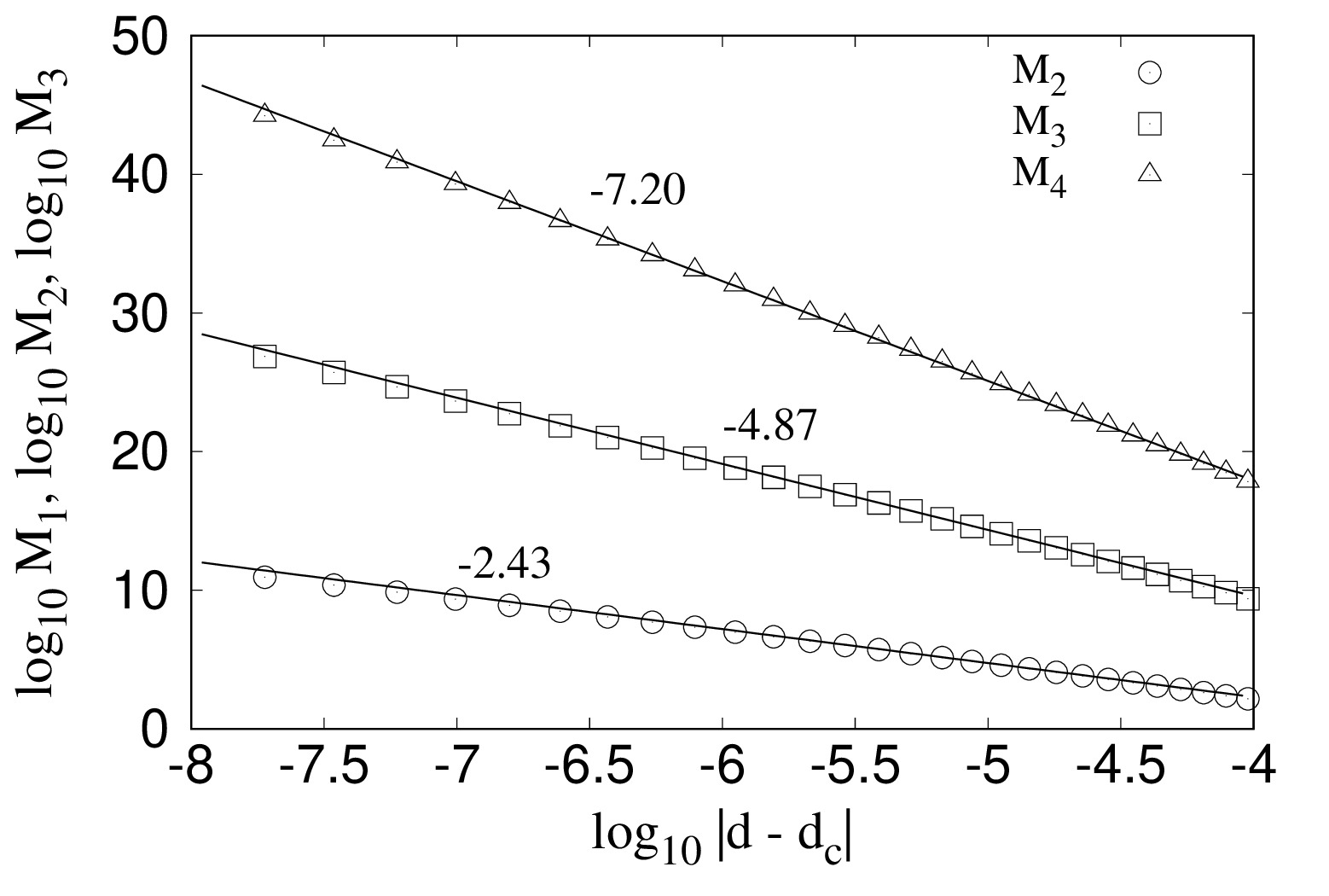
Figure 6: Plot of the second, third and fourth moments $M_{2}$, $M_{3}$ and $M_{4}$ of cluster size distribution function as a function of $|d-d_{c}|$ for $T=0.06$ and $f=0.10$. From the slopes, we obtain the exponents, $\gamma=2.43\pm 0.03$, $\delta=4.87\pm 0.05$ and $\eta=7.20\pm 0.07$.

Applied stress ($f$)	$0.10$	$0.12$	$0.14$	$0.16$	$0.18$
$d_{c}$	$0.543\pm 0.001$	$0.537\pm 0.001$	$0.522\pm 0.001$	$0.503\pm 0.001$	$0.485\pm 0.001$
$\beta$	$0.20\pm 0.05$	$0.19\pm 0.06$	$0.21\pm 0.04$	$0.23\pm 0.07$	$0.18\pm 0.05$
$\gamma$	$2.43\pm 0.03$	$2.40\pm 0.04$	$2.39\pm 0.03$	$2.45\pm 0.02$	$2.44\pm 0.02$
$\delta$	$4.87\pm 0.05$	$4.83\pm 0.04$	$4.89\pm 0.03$	$4.88\pm 0.02$	$4.92\pm 0.02$
$\eta$	$7.20\pm 0.07$	$7.23\pm 0.09$	$7.15\pm 0.08$	$7.20\pm 0.09$	$7.19\pm 0.07$
$\tau$	$2.06\pm 0.05$	$2.03\pm 0.04$	$2.07\pm 0.04$	$2.06\pm 0.02$	$2.10\pm 0.03$
$\sigma$	$0.40\pm 0.02$	$0.39\pm 0.04$	$0.43\pm 0.03$	$0.41\pm 0.02$	$0.38\pm 0.03$
$\delta$ (Eq. 13)	$5.06\pm 0.11$	$4.99\pm 0.14$	$4.99\pm 0.10$	$5.13\pm 0.11$	$5.06\pm 0.09$
$\eta$ (Eq. 13)	$7.31\pm 0.13$	$7.26\pm 0.12$	$7.39\pm 0.09$	$7.31\pm 0.06$	$7.40\pm 0.06$
$\sigma$ (Eq. 12)	$0.37\pm 0.12$	$0.34\pm 0.16$	$0.38\pm 0.12$	$0.36\pm 0.14$	$0.43\pm 0.15$

Table 1: List of the threshold damage and critical exponents obtained for different applied stress in the non-localized regime. Exponents are close to those observed in 2D percolation model where $\beta=5/36$, $\gamma=43/18$, $\tau=187/91$ and $\sigma=36/91$. We also show in the bottom three rows the calculation of $\eta$, $\delta$ and $\sigma$ by using the scaling relations in Eqs. 12 and 13 which can be compared with the measured values of the exponents.

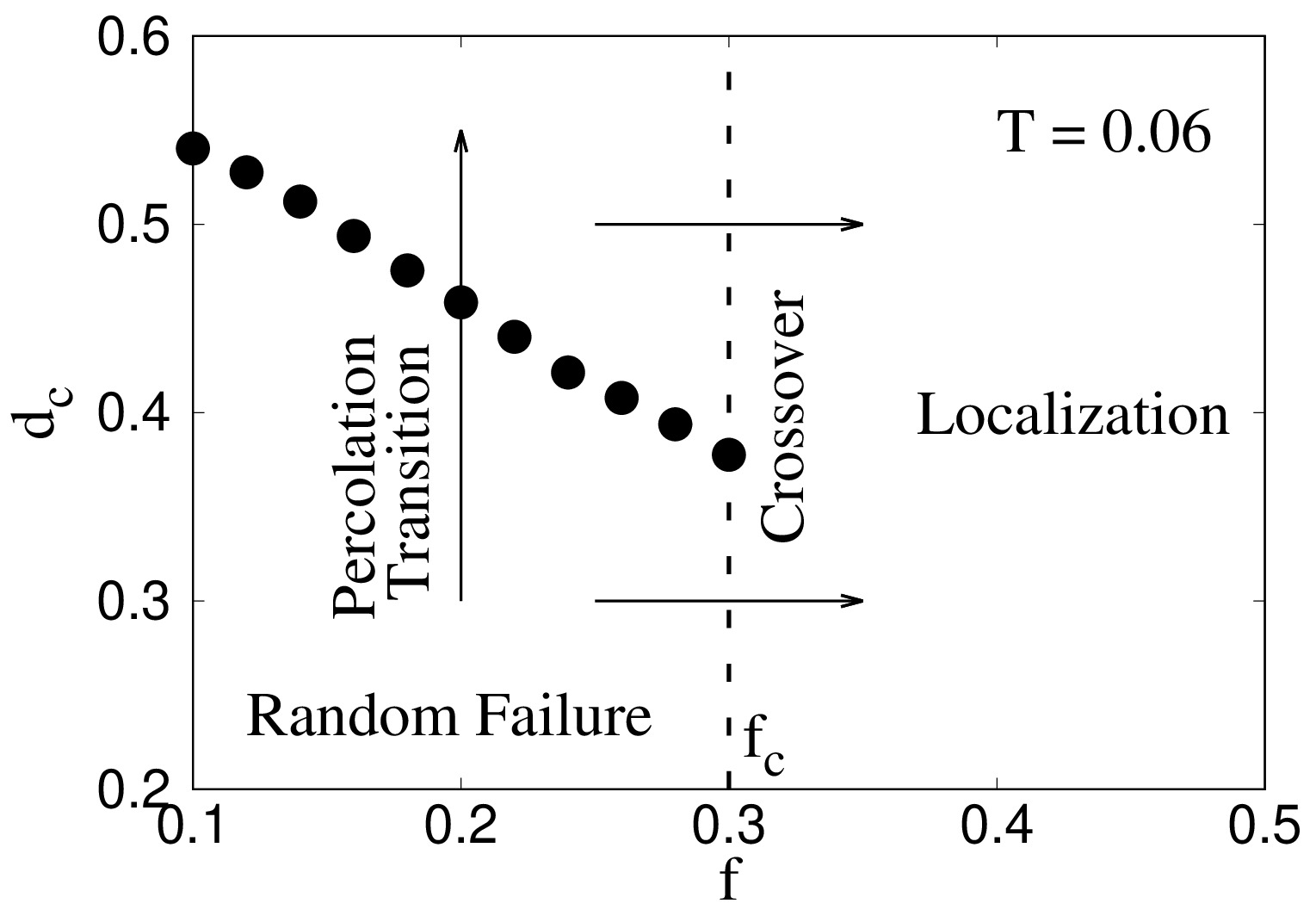
Figure 7: The figure shows two different regions: (I) random failure and (II) localization, depending on whether the stress applied on the model is below or above $f_{t}$ (the crossover point). For $f>f_{c}$, individual patches grows within the bundle. For $f<f_{c}$, the failure process is random and the model undergoes a percolation transition around damage $d_{c}$. We keep $T=0.06$ and $D=0.02$.

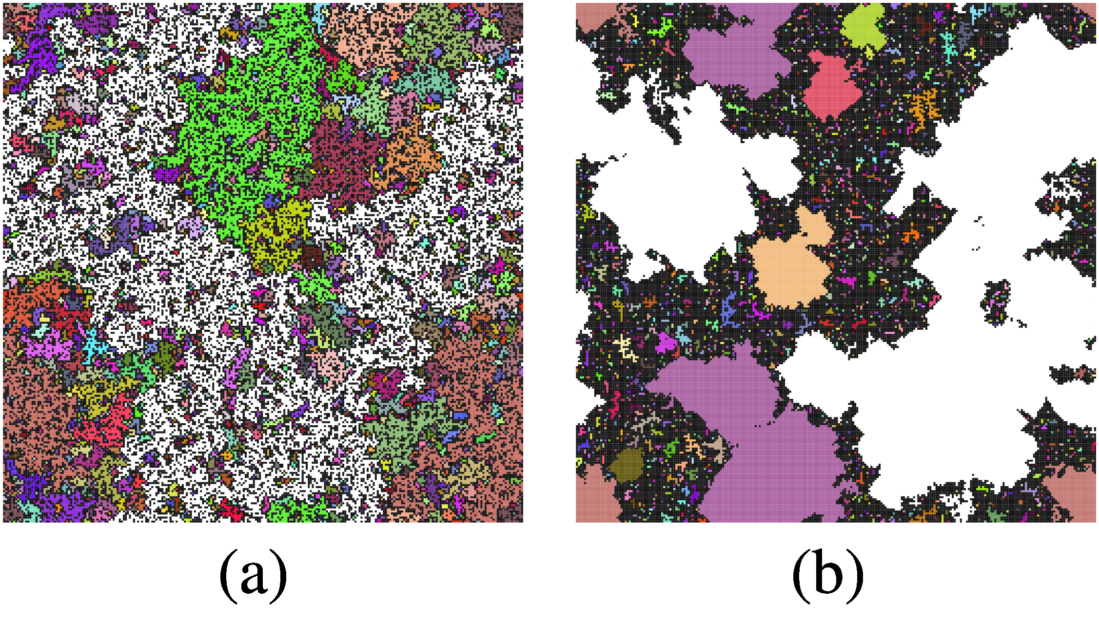
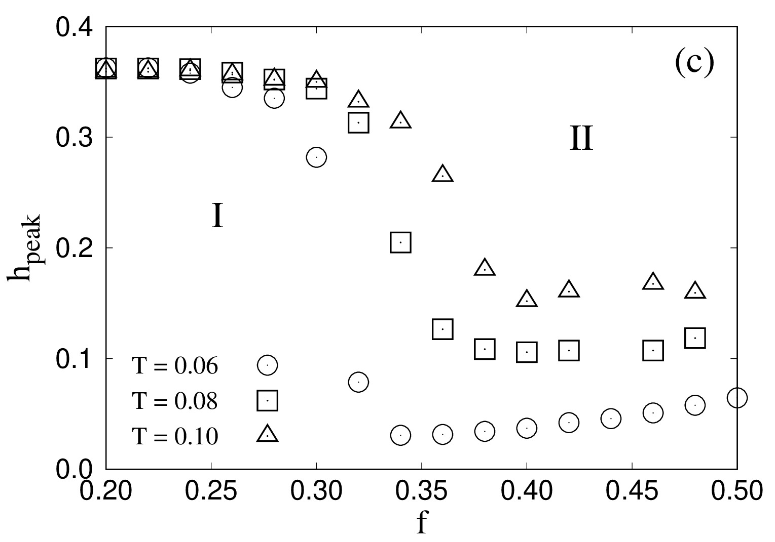
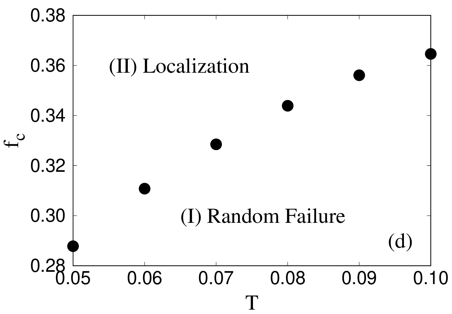
Figure 8: Snapshots of the system for (a) non-localized ($f=0.1$) and (b) localized ($f=0.4$) growths when a spanning cluster appears in the system. The largest cluster is marked by white. In (c), we show the variation of $h_{\rm peak}$ with applied stress $f$ where $h_{\rm peak}$ has a high value at low applied stress. As $f$ is increased beyond a threshold value $f_{c}$, $h_{\rm peak}$ decreases rapidly and saturates at sufficiently low value. In (d) we show the boundary separating two different regimes, (I) the percolation type random failure and (II) the localized crack growth. As temperature increases, the localization takes place at a relatively higher applied stress as the stress concentration has to overcome a larger thermal randomness.

3.3 Boundary between the random and localized failure

We show in Fig. 7, the variation of the critical damage $d_{c}$ with the applied stress $f$ for $T=0.06$. The system undergoes a percolation transition at $d_{c}$. The value of $d_{c}$ decreases with the increase in $f$ for $f<f_{c}$. Above $f_{c}$, there is a crossover in the failure process from a percolation type growth to a compact localized growth where the geometrical quantities show different behavior as observed in Fig. 3. To find the boundary that separates the random failure from the localized fracture growth as a function of temperature, we focus on the largest perimeter size $h_{\rm max}$ which shows abrupt decrease in the peak value when the applied stress crosses $f_{c}$. As mentioned before, this is due to the fractal structure of the percolation clusters at $d_{c}$ which makes the hull highly rarefied and long compared to the perimeters of the compact clusters in the localized growth. Two such clusters are shown in Fig. 8 (a) and (b) for the percolation type growth and the localized growth respectively where the largest clusters are colored by white. In Fig. 8 (c), we plot $h_{\rm peak}$, the maximum value of the largest perimeter size $h_{\rm max}$ during a failure process, as a function of the applied stress $f$ for three different temperatures $T=0.06$, $0.08$ and $0.10$. The plots show two distinct regimes, a regime (I) with fairly constant higher values, then another regime (II) where $h_{\rm peak}$ falls rapidly to a relatively lower value as $f$ crosses $f_{c}$. By measuring the values of $f_{c}$ for different temperatures, we find the boundary on the $f_{c}$ vs $T$ plane that separates the random failure (I) from the localized failure process (II). As temperature is increased, a higher applied stress is required to establish localization in the model. This is because the increase in temperature increases thermal fluctuations that lead to higher spatial randomness in the failure events. In this case, a large amount of stress localization is required to counteract the thermal fluctuation.

4 Conclusions

We have included thermal noise in an LLS fiber bundle model to study creep and subsequent failure through the interplay between thermal fluctuations and stress concentration due to externally applied stress. We observed that the presence of thermal fluctuations makes the failure events spatially uncorrelated and non-localized even if the strength of system disorder is low. This non-localized fracture growth shows a percolation transition governed by critical exponents and scaling relations. In the absence of temperature, the same amount of system disorder shows a highly correlated failure process in LLS fiber bundle model [43]. Such spatial correlation can be obtained in presence of temperature as well when the applied stress is sufficiently high so that the effect of stress localization can outrun the effect of thermal fluctuations. This is a new mechanism for establishing localization. Stormo et. al [36] observed localized failure in a soft clamp model [35] as the elasticity of the clamps are decreased. In fiber bundle model the disorder strength and the stress release range plays a crucial role in determining the correlations in space. It was recently shown [43] that as the strength of disorder is tuned, a percolation transition is observed from a localized phase to a non-localized phase. One can also approach a random failure process if the stress release range is increased [47, 48] instead of the disorder strength. In the present study, we show that as the temperature is increased, a larger stress has to be applied to overcome the thermal fluctuations and to initiate the localization. In this work, however, we have not addressed the combined effect of varying both the thermal noise and system disorder during the failure process, which will be interesting to study in the future.

References

- [1] H. J. Herrmann and S. Roux Eds., Statistical models for the fracture of disordered media (Elsevier, Amsterdam, 2014).
- [2] B. R. Lawn, Fracture of Brittle Solids (Cambridge University Press, Cambridge, 1993).
- [3] T. Wong and P. Baud, The brittle-ductile transition in porous rock: A review, J. Struct. Geol. 44, 25 (2012).
- [4] H. Charan, A. Hansen, H. G. E. Hentschel and I. Procaccia, Fatigue and failure of a polymer chain under tension, arXiv:2008.00970 (2020).
- [5] B. Voight, A relation to describe rate-dependent material failure, Science 243, 200 (1989).
- [6] I. G. Main, A damage mechanics model for power-law creep and earthquake aftershock and foreshock sequences, Geophys. J. Int. 142, 151 (2000).
- [7] H. Nechad, A. Helmstetter, R. El. Guerjouma and D. Sornette, Andrade and critical time-to-failure laws in fiber-matrix composites: Experiments and model, J. Mech. Phys. Solids 53, 1099 (2005).
- [8] S. Ciliberto, A. Guarino and R. Scorretti, The effect of disorder on the fracture nucleation process, Physica D 158, 83 (2001).
- [9] R. Scorretti, S. Ciliberto and A. Guarino, Disorder enhances the effects of thermal noise in the fiber bundle model, Eurphys. Lett. 55, 626 (2001).
- [10] A. Politi, S. Ciliberto and R. Scorretti, Failure time in the fiber-bundle model with thermal noise and disorder, Phys. Rev. E 66, 026107 (2002).
- [11] A. Saichev and D. Sornette, Andrade, Omori, and time-to-failure laws from thermal noise in material rupture, Phys. Rev. E 71, 016608 (2005).
- [12] R. C. Hidalgo, Y. Moreno, F. Kun and H. J. Herrmann, Fracture model with variable range of interaction, Phys. Rev. E 65, 046148 (2002).
- [13] R. C. Hidalgo, F. Kun and H. J. Herrmann, Bursts in a fiber bundle model with continuous damage, Phys. Rev. E 64, 066122 (2001).
- [14] R. C. Hidalgo, F. Kun and H. J. Herrmann, Creep rupture of viscoelastic fiber bundles, Phys. Rev. E 65, 032502 (2002).
- [15] F. Kun, Y. Moreno, R. C. Hidalgo and H. J. Herrmann, Creep rupture has two universality classes, Europhys. Lett. 63, 347 (2003).
- [16] S. Pradhan and B. K. Chakrabarti, Failure due to fatigue in fiber bundles and solids, Phys. Rev. E 67, 046124 (2003).
- [17] Z. Danku and F. Kun, Creep rupture as a non-homogeneous Poissonian process, Sci. Rep. 3, 2688 (2013).
- [18] S. Pradhan, A. K. Chandra and B. K. Chakrabarti, Noise-induced rupture process: Phase boundary and scaling of waiting time distribution, Phys. Rev. E 88, 012123 (2013).
- [19] F. T. Peirce, Tensile Tests for Cotton Yarns: Theorems on the Strength of Long and of Composite Specimens, J. Text. Ind. 17, 355 (1926).
- [20] H. E. Daniels, The statistical theory of the strength of bundles of threads. I, Proc. R. Soc. London Ser. A 183, 405 (1945).
- [21] H. J. Herrmann and S. Roux, Statistical Models for the Fracture of Disordered Media (North Holland, Amsterdam, 1990).
- [22] B. K. Chakrabarti and L. G. Benguigui, Statistical Physics of Fracture and Breakdown in Disordered Systems (Oxford University Press, Oxford, 1997).
- [23] S. Pradhan, A. Hansen and B. K. Chakrabarti, Failure processes in elastic fiber bundles, Rev. Mod. Phys. 82, 499 (2010).
- [24] A. Hansen, P. C. Hemmer and S. Pradhan, The Fiber Bundle Model: Modeling Failure in Materials, WILEY-VCH (2015).
- [25] S. Biswas, P. Ray and B. K. Chakrabarti, Statistical Physics of Fracture, Beakdown, and Earthquake: Effects of Disorder and Heterogeneity, WILEY-VCH (2015).
- [26] S. Roy, S. Biswas and P. Ray, Failure time in heterogeneous systems, Phys. Rev. Res. 1, 033047 (2019).
- [27] S. Roy and T. Hatano, Creeplike behavior in athermal threshold dynamics: Effects of disorder and stress, Phys. Rev. E 97, 062149 (2018).
- [28] D. Sornette, Mean-field solution of a block-spring model of earthquakes, J. Phys. I France 2, 2089 (1992).
- [29] P. C. Hemmer and A. Hansen, The distribution of simultaneous fiber failures in fiber bundles, J. Appl. Mech. 59, 909 (1992).
- [30] A. Hansen and P. C. Hemmer, Burst avalanches in bundles of fibers: Local versus global load-sharing, Phys. Lett. A 184, 394 (1994).
- [31] S. D. Zhang and E. J. Ding, Burst-size distribution in fiber-bundles with local load-sharing, Phys. Lett. A 193, 425 (1994).
- [32] M. Kloster, A. Hansen and P. C. Hemmer, Burst avalanches in solvable models of fibrous materials, Phys. Rev. E 56, 2615 (1997).
- [33] D. G. Harlow and S. L. Phoenix, The Chain-of-Bundles Probability Model for the Strength of Fibrous Materials II: A Numerical Study of Convergence, J. Compos. Mater. 12, 314 (1978).
- [34] D. G. Harlow and S. L. Phoenix, Approximations for the strength distribution and size effect in an idealized lattice model of material breakdown, J. Mech. Phys. Solids 39, 173 (1991).
- [35] G. G. Batrouni, A. Hansen and J. Schmittbuhl, Heterogeneous interfacial failure between two elastic blocks, Phys. Rev. E 65, 036126 (2002).
- [36] A. Stormo, K. S. Gjerden and A. Hansen, Onset of localization in heterogeneous interfacial failure, Phys. Rev. E 86, 025101(R) (2012).
- [37] K. S. Gjerden, A. Stormo and A. Hansen, Universality Classes in Constrained Crack Growth, Phys. Rev. Lett. 111, 135502 (2013).
- [38] K. S. Gjerden, A. Stormo and A. Hansen, Local dynamics of a randomly pinned crack front: a numerical study, Front. Phys. 2, 66 (2014).
- [39] S. Sinha, J. T. Kjellstadli and A. Hansen, Local load-sharing fiber bundle model in higher dimensions, Phys. Rev. E 92, 020401 (2015).
- [40] D. Stauffer, Scaling theory of percolation clusters, Phys. Rep. 54, 1 (1979).
- [41] D. Stauffer and A. Aharony, Introduction to Percolation Theory, 2nd ed. (Taylor and Francis, London, 1995).
- [42] T. Grossman and A. Aharony, Accessible external perimeters of percolation clusters, J. Phys. A: Math. Gen. 20, L1193 (1987).
- [43] S. Sinha, S. Roy and A. Hansen, Phase transitions and correlations in fracture processes where disorder and stress compete, arXiv:2005.11620 (2020).
- [44] S. Roy and T. Hatano, Creep failure in a threshold-activated dynamics: Role of temperature during a subcritical loading, Phys. Rev. Res. 2, 023104 (2020).
- [45] A. Hansen, E. L. Hinrichsen and S. Roux, Scale-invariant disorder in fracture and related breakdown phenomena, Phys. Rev. B 43, 665 (1991).
- [46] B. Skjetne and A. Hansen, Implications of Realistic Fracture Criteria on Crack Morphology, Front. Phys. 7, 50 (2019).
- [47] S. Biswas, S. Roy and P. Ray, Nucleation versus percolation: Scaling criterion for failure in disordered solids, Phys. Rev. E 91, 050105(R) (2015).
- [48] S. Roy, S. Biswas and P. Ray, Modes of failure in disordered solids, Phys. Rev. E 96, 063003 (2017).