Stable and self-consistent compact star models in teleparallel gravity

Abstract

In the framework of Teleparallel Gravity, we derive a charged non-vacuum solution for a physically symmetric tetrad field with two unknown functions of radial coordinate. The field equations result in a closed-form adopting particular metric potentials and a suitable anisotropy function combined with the charge. Under these circumstances, it is possible to obtain a set of configurations compatible with observed pulsars. Specifically, boundary conditions for the interior spacetime are applied to the exterior Reissner-Nordström metric to constrain the radial pressure that has to vanish through the boundary. Starting from these considerations, we are able to fix the model parameters. The pulsar PSR J 1614–2230, with estimated mass $M=1.97\pm 0.04\,M_{\circledcirc},$ and radius $R=9.69\pm 0.2$ km is used to test numerically the model. The stability is studied, through the causality conditions and adiabatic index, adopting the Tolman-Oppenheimer-Volkov equation. The mass-radius $(M,R)$ relation is derived. Furthermore, the compatibility of the model with other observed pulsars is also studied. We reasonably conclude that the model can represent realistic compact objects.

I Introduction

Soon after the formulation of General Relativity (GR), several theories were constructed in view of fixing as many issues as possible related to the gravitational field. Among these theories, there is the one formulated by H. Weyl which tried to unify gravitation and electromagnetism in 1918 Weyl (1918). Einstein himself, in 1928 Einstein (2006), adopted the same philosophy by Weyl adopting the Weitzenböck geometry. In this formulation, one has to introduce tetrad fields to describe dynamics, unlike GR whose dynamical variable is the metric. The tetrad field has 16 components which made Einstein think that the extra 6 components, with respect to the metric, could describe the components of the electromagnetic field. Nevertheless, it was shown that these extra 6 components are linked to the local Lorentz invariance of the theory Mueller-Hoissen and Nitsch (1983); Capozziello et al. (2014).

Despite the failure of the Weyl and Einstein attempts, the new approaches supplied the notion of gauge theory and thus the search for a gauge gravity started O’Raifeartaigh (1997); Blagojević and Hehl (2013). In 1979, K. Hayashi and T. Shirafuji Hayashi and Shirafuji (1979) proposed a gravitational theory, called “New General Relativity” that is a gauge theory for the translation group. This theory involves three free parameters to be determined by the experiment.

Another theory that is built up through the Weitzenböck geometry is the Teleparallel Equivalent of General Relativity (TEGR). TEGR and GR are equivalent at the level of field equations however, at the level of actions, they are different for a total divergence term Maluf (2013); Wu and Geng (2012); Capozziello et al. (2020); Awad et al. (2018a, 2017); El Hanafy and Nashed (2016a). In TEGR, gravity is encoded in the torsion field, with vanishing curvature, unlike GR where gravity is encoded in metric and curvature fields with vanishing torsion Li et al. (2011); Shirafuji and Nashed (1997); El Hanafy and Nashed (2016b); Nashed (2011); Krššák (2017); Nashed (2003); Awad et al. (2018b); Bahamonde et al. (2015); Cai et al. (2016).

In this situation, a good approach could be testing different formulations of gravitational interaction by searching for signatures discriminating among concurrent theories. Systems, in strong field regime, are natural candidates to this aim. Signatures can come from compact objects like neutron stars or black holes, or from polarizations of gravitational waves Bogdanos et al. (2010); Abedi and Capozziello (2018); Capozziello et al. (2020, 2019).

From a physical point of view, compact objects are, in general, stars exhausting their nuclear fuel. They can give rise to stable compact objects or to black holes. For example, neutron stars are compact objects which are boosted by their neutron degeneracy pressure against the attraction of gravity. Another type of compact stars are the white dwarfs, boosted by the electron degeneracy pressure against the gravity.

From a theoretical viewpoint, it is well know that the first exact vacuum solution of GR was the Schwarzschild one Schwarzschild (1916). Thereafter many solutions investigating compact stars have been proposed. In particular, searching for interior solutions, describing realistic compact objects, became a fertile domain to probe GR and other theories. Using the equation of state (EoS), one can study the stability structure of compact stellar objects and then guess on their internal composition. Specifically, the EoS is useful to investigate the physical behavior of the stellar structure through the Tolman-Oppenheimer-Volkov (TOV) equation which is the general relativistic equation of the stellar interior coming from the internal Schwarzschild solution.

In order to study stellar configurations, one can assumes, at the beginning, that the distribution of matter is isotropic which means that the radial and tangential pressures are equal. However, in realistic cases, such assumption does not hold and one finds that the two components of radial and tangential pressures are not equal: the differences between them create the anisotropy. Such stellar configurations have unequal radial and tangential pressures. Lemaître, in 1933, was the first which proposed anisotropic models Lemaitre (1997). Moreover, it possible to show that, in order to reach stable configurations, at the maximal star surface, the radial pressure has to decrease and, at the center, it has to vanish Mak and Harko (2004a, b).

There are several factors to be taken into account to study anisotropic stars; among these, the high density regime where the nuclear interactions have to be relativistically treated Ruderman (1972); Canuto (1975). Moreover the existence of a solid core or a 3A type superfluid may cause the star to be anisotropic Kippenhahn et al. (2013). There is another source that makes the star anisotropic: it is a strong magnetic field Tamta and Fuloria (2017); Astashenok et al. (2015a). The slow rotation can be considered another source of anisotropy Herrera and Santos (1994). Letelier showed that combinations between perfect and null fluids can give rise to anisotropic fluids Letelier (1980). Other reasons can be taken into account to generate anisotropies like pion condensation Sawyer (1972), strong electromagnetic field Usov (2004) and phase transition Sokolov (1980).

Dev and Gleiser Dev and Gleiser (2003, 2002) and Gleiser and Dev Gleiser and Dev (2004) investigated the operators that induce the pressure to be anisotropic. It was shown that the effect of shear, electromagnetic field, etc. on self-bound systems can be neglected, if the system is anisotropic Ivanov (2010). Systems that consist of scalar fields like boson stars possess anisotropy Schunck and Mielke (2003). Gravastars and wormholes can be considered as anisotropic models Morris and Thorne (1988); Cattoen et al. (2005); DeBenedictis et al. (2006); De Falco et al. (2020). An application of anisotropic model to stable configurations of neutron stars has been discussed in Bowers and Liang (1974). They showed that anisotropy might have non-negligible effects on the equilibrium mass and on the surface red-shift.

A nice study describing the origin and the effects of anisotropy can be found in Chan et al. (2003); Herrera and Santos (1997). Super dense and anisotropic neutron stars have been considered and a conclusion is that there is no limiting mass of such stars Heintzmann and Hillebrandt (1975).

Supermassive neutron stars in alternative gravity are considered, for example, in Astashenok et al. (2015b, 2014, 2013); Capozziello et al. (2016). The presence of torsion field in neutron star models is studied in Feola et al. (2020). The issue of stability of anisotropic stars has been analyzed in etd and a conclusion is that the stability of such systems is similar to that of isotropic stars.

There are many anisotropic models that deal with the anisotropic pressure in the energy-momentum tensor. Several exact spherically symmetric solutions of interior stellar have been developed Bayin (1982); Krori et al. (1984); Bondi (1993, 1999); Barreto (1993); Barreto et al. (2007); Coley and Tupper (1994); Martinez et al. (1994); Singh et al. (1995); Hernández et al. (1999); Harko and Mak (2000); Patel and Mehta (1995); Lake (2004); Böhmer and Harko (2006); Boehmer and Harko (2007); Esculpi et al. (2007); Khadekar and Tade (2007); Karmakar et al. (2007); Abreu et al. (2007); IVANOV (2010); Herrera et al. (2009); Mak and Harko (2003); Sharma and Mukherjee (2002); Maharaj and Maartens (1989); Chaisi and Maharaj (2006); Herrera et al. (2008); Chaisi and Maharaj (2005); Gokhroo and Mehra (1994); Lake (2009); V O et al. (2012); Thomas and Ratanpal (2007); Tikekar and Thomas (2005); Thirukkanesh and Maharaj (2008a, b); Sharma and Ratanpal (2013); Pandya et al. (2015); Bhar et al. (2015).

Beside this, adding charge effects in compact objects is an issue widely considered in literature, especially for neutron and quark stars Bekenstein (1971); Dionysiou (1985); Ray et al. (2003); Ghezzi (2005); Lasky and Lun (2007); Negreiros et al. (2009). An important result is the fact that the distribution of net charge can improve the maximum mass of compact stars. For example for white dwarfs, there are several results related to the charge effects affecting the structure (see, e.g. Olson and Bailyn (1976)). For this reason, we consider here charged compact star models showing that the net charge effects can increase the maximum mass.

The aim of the present paper is to derive a novel charged anisotropic solution in the framework of TEGR and compare it with realistic stellar configurations using physical assumptions on the form of metric potential and the combination of charge and anisotropy. In particular, we consider the pulsar PSR J 1614 - 2230 which estimated mass $M=1.97\pm 0.04M_{\circledcirc}$ and radius is $R=9.69\pm 0.2$ km Demorest et al. (2010). This peculiar system escapes the standard GR explanation of neutron stars because it is too massive to be stable unless one assumes exotic EoS or alternative gravities. We discuss the physical parameters of such a pulsar considering our solution derived in the framework of TEGR. From our point of view, this can constitute a possible test for the theory.

The set up of the paper is the following. In Sec. II, we sketch the TEGR theory in presence of the electromagnetic field. Sec. III is devoted to the discussion of charged compact stars in TEGR. The requirements for a physically consistent stellar model in TEGR are discussed in Sec. IV. The physical properties of the model are considered in Sec.V. The model is matched with realistic compact stars, in particular with PSR J 1614–2230, in Sec. VI. In Sec.VII, the stability of the model is taken into account with respect to the TOV equation and the adiabatic index. In particular, we report the $(M,R)$ relation and how it is affected by the electromagnetic field. Discussion and conclusions are reported in Sec. VIII.

II Teleparallel equivalent of general relativity and the electromagnetic field

In TEGR theory, at each point of the spacetime manifold, $M$, can be defined a tangent Minkowski spacetime $\eta_{ij}=(+1,-1,-1,-1)$. As is well-known that the dynamical fields of TEGR are the four linearly independent vierbeins (tetrads) from where we can define the metric and its inverse as

$$g_{\mu\nu}=\eta_{ab}l^{a}{}_{\mu}l^{b}{}_{\nu}\,,\qquad\qquad g^{\mu\nu}=\eta^{ab}L_{a}{}^{\mu}L_{b}{}^{\nu}\,,$$ (1)

with $\eta_{ab}$ being the flat Minkowski metric of the tangent space and $l^{b}{}_{\nu}$, $L_{b}{}^{\nu}$ are the covariant and contra-variant tetrad fields. Using Eq. (1) we can define the following orthogonal conditions

$$L_{i}{}^{\mu}l^{i}{}_{\nu} =\delta^{\nu}_{\mu}, l^{i}{}_{\mu}L_{j}{}^{\mu} =\delta^{i}_{j}\,.$$ (2)

From the above definitions, we can define the torsion tensor as

$$T^{a}{}_{\mu\nu}=2\left(\partial_{[\mu}l^{a}{}_{\nu]}+\omega^{a}{}_{b[\mu}l^{b}{}_{\nu]}\right)\,.$$ (3)

where $\omega^{a}{}_{b\mu}$ is the spin connection which we can set equal zero due to TEGR. Therefore the torsion tensor (3) reduces to

$$T^{a}{}_{\mu\nu}=\partial_{[\mu}l^{a}{}_{\nu]}.$$ (4)

TEGR with electromagnetic field is recovered from the action

$$S_{\rm TEGR}=\int\mathrm{d}^{4}x\ |l|\left(\frac{1}{2\kappa^{2}}T+\mathcal{{\cal F}}\right)\,,$$ (5)

where $\kappa^{2}=8\pi$, $|l|=\det(l^{a}{}_{\mu})=\sqrt{-g}$ is the determinant of the tetrad field, ${\cal{\cal F}}$ is a gauge-invariant scalar defined as ${\cal F}=\frac{1}{4}{\cal F}_{\alpha\beta}{\cal F}^{\alpha\beta}$ Plebański (1970); Nashed (2006a). The torsion scalar $T$ is defined as

$$T=T^{a}{}_{\mu\nu}S_{a}{}^{\mu\nu}=\frac{1}{2}\left(L_{a}{}^{\sigma}g^{\rho\mu}L_{b}{}^{\nu}+2L_{b}{}^{\rho}g^{\sigma\mu}L_{a}{}^{\nu}+\frac{1}{2}\eta_{ab}g^{\mu\rho}g^{\nu\sigma}\right)T^{a}{}_{\mu\nu}T^{b}{}_{\rho\sigma}\,,$$ (6)

where $S_{a}{}^{\mu\nu}$ is the superpotential defined as

$$S_{a}{}^{\mu\nu}=\frac{1}{2}(K^{\mu\nu}{}_{a}-L_{a}{}^{\mu}T_{\lambda}{}^{\lambda\nu}+L_{a}{}^{\nu}T_{\lambda}{}^{\lambda\mu})$$ (7)

in terms of the contortion tensor

$$K^{\mu\nu}{}_{a}=\frac{1}{2}(T^{\nu\mu}{}_{a}+T_{a}{}^{\mu\nu}-T^{\mu\nu}{}_{a})\,.$$ (8)

The metric components are functions of the tetrads. The variation with respect to the tetrad $l^{a}{}_{\mu}$ yields the field equations (see Krššák and Saridakis (2016) for details)

$$\frac{1}{4}TL_{a}{}^{\mu}+T^{b}{}_{\nu a}S_{b}{}^{\mu\nu}+\frac{1}{h}\partial_{\nu}(lS_{a}{}^{\mu\nu}) =\frac{1}{2}\kappa^{2}{\cal T}_{a}{}^{\mu}\,.$$ (9)

The stress-energy tensor ${\cal T}_{a}{}^{\mu}$ consists of two terms

$${\cal T}_{a}{}^{\mu}\>={\cal T}_{a}{}^{\mu}{}_{AF}+{\cal T}_{a}{}^{\mu}_{EM},$$ (10)

where

$${\cal T}_{a}{}^{\mu}{}_{AF}=(p_{t}+\rho)u^{\mu}u_{a}+p_{t}\delta_{a}{}^{\mu}+(p_{r}-p_{t})\xi_{a}\xi^{\mu}\,,$$ (11)

is the energy-momentum tensor of an anisotropic fluid, and

$${\cal T}_{a}{}^{\mu}{}_{EM}=\frac{1}{4}\left({\cal F}_{a\alpha}{\cal F}^{\mu\alpha}-\frac{1}{4}\delta_{a}{}^{\mu}{\cal F}_{\alpha\beta}{\cal F}^{\alpha\beta}\right)\,,$$ (12)

is the energy-momentum tensor of the electromagnetic field. Here $u_{\mu}$ is the time-like vector defined as $u^{\mu}=[1,0,0,0]$ and $\xi_{\mu}$ is the unit space-like vector in the radial direction defined as $\xi^{\mu}=[0,1,0,0]$ such that $u^{\mu}u_{\mu}=-1$ and $\xi^{\mu}\xi_{\mu}=1$. In this paper, $\rho$ is the energy-density, $p_{r}$ and $p_{t}$ are the radial and the tangential pressures respectively. Furthermore, the electromagnetic tensor $F_{\mu\nu}$ satisfies the Maxwell equations

$$F_{\mu\nu,\gamma}+F_{\nu\gamma,\mu}+F_{\gamma\mu,\nu}=0,$$

$$\left(\sqrt{-g}F^{\mu\nu}\right)_{\,,\nu}=4\pi J^{\mu}\sqrt{-g},$$ (13)

where $J^{\mu}=\sigma u^{\mu}$ is the current density and $\sigma$ is the charge density. In the next section, we are going to apply the field equations (9) and (II) to a spherically symmetric tetrad space and try to solve the resulting system of differential equations.

III Charged compact stars

Let us begin with the following spherically symmetric metric using the spherical coordinates $(t,r,\theta,\phi)$

$$ds^{2}=-G(r)\,dt^{2}+H(r)dr^{2}+r^{2}(d\theta^{2}+\sin^{2}\theta d\phi^{2})\,,$$ (14)

where $G(r)$ and $H(r)$ are two unknown functions depending on the radial coordinate $r$. The above metric (14) can be reproduced from the following covariant tetrad field  Bahamonde et al. (2019)

$$l^{a}{}_{\mu}=\left(\begin{array}[]{cccc}\sqrt{G(r)}&0&0&0\\ 0&\sqrt{H(r)}\cos(\phi)\sin(\theta)&r\cos(\phi)\cos(\theta)&-r\sin(\phi)\sin(\theta)\\ 0&\sqrt{H(r)}\sin(\phi)\sin(\theta)&r\sin(\phi)\cos(\theta)&r\cos(\phi)\sin(\theta)\\ 0&\sqrt{H(r)}\cos(\theta)&-r\sin(\theta)&0\\ \end{array}\right)\,.$$ (15)

The tetrad (15) is the output of the product of a diagonal tetrad and a local Lorentz transformation which can be written as

$$l^{a}{}_{\mu}=\Lambda^{a}{}_{b}l^{b}{}_{\mu_{diag}}$$

$$\Rightarrow\left(\begin{array}[]{cccc}\sqrt{G(r)}&0&0&0\\ 0&\sqrt{H(r)}\cos(\phi)\sin(\theta)&r\cos(\phi)\cos(\theta)&-r\sin(\phi)\sin(\theta)\\ 0&\sqrt{H(r)}\sin(\phi)\sin(\theta)&r\sin(\phi)\cos(\theta)&r\cos(\phi)\sin(\theta)\\ 0&\sqrt{H(r)}\cos(\theta)&-r\sin(\theta)&0\\ \end{array}\right)$$ (20)

$$\equiv\underbrace{\left(\begin{array}[]{cccc}1&0&0&0\\ 0&\cos(\phi)\sin(\theta)&\cos(\phi)\cos(\theta)&-\sin(\phi)\\ 0&\sin(\phi)\sin(\theta)&\sin(\phi)\cos(\theta)&\cos(\phi)\\ 0&\cos(\theta)&-\sin(\theta)&0\\ \end{array}\right)}_{Local\,\,Lorentz\,\,transformation}\times\underbrace{\left(\begin{array}[]{cccc}\sqrt{G(r)}&0&0&0\\ 0&\sqrt{H(r)}&0&0\\ 0&0&r&0\\ 0&0&0&r\sin(\theta)\\ \end{array}\right)}_{Diagonal\,\,tetrad}\,.$$ (29)

It is worth noticing that the diagonal tetrad can be applied to the field equations of $f(T)$ TEGR models Bahamonde et al. (2019). Here we shall take into account the effect of local Lorentz transformation given by Eq. (29) and see if the results are different from those presented in Newton Singh et al. (2019).

Using Eq. (15) into Eq. (6), the torsion scalar takes the form

$$T=\frac{2\left(2G\sqrt{H}-GH+r\sqrt{H}G^{\prime}-G-rG^{\prime}\right)}{GHr^{2}}\,.$$ (30)

Despite the fact that the diagonal tetrad in Eq. (III) and tetrad (15) reproduce the same metric, their torsion scalars are different. The reason for this difference is the Local Lorentz transformation (LLT) in (III). The torsion scalar of Eq. (30) goes to zero when both the unknown functions $G(r)$ and $H(r)$ tend to one, which is the necessary condition to achieve the asymptotic flatness. Nevertheless, the torsion scalar presented in Newton Singh et al. (2019) does not vanish as it should when we apply the same condition. So the existence of LLT makes our torsion scalar more physically motivated.

Using Eq. (30) into field Eqs. (9) and (II), we get

$$-8\pi\rho+E^{2}(r) = \frac{H[1-H]-rH^{\prime}}{r^{2}H^{2}}\,,$$

$$8\pi p_{r}+E^{2}(r) = \frac{rG^{\prime}-G(H-1)}{2r^{2}GH}\,,$$

$$8\pi p_{t}-E^{2}(r) = \frac{2GH[G^{\prime}+rG^{\prime\prime}]-rHG^{\prime 2}-2G^{2}H^{\prime}-rGG^{\prime}H^{\prime}}{8rG^{2}H^{2}}\,,$$ (31)

$$\Delta(r) = \frac{r^{2}H[2GG^{\prime\prime}-G^{\prime 2}]-rGG^{\prime}[2H+rH^{\prime}]-2G^{2}[2H(1-H)+rH^{\prime}]}{8r^{2}G^{2}H^{2}}+2E^{2}(r)\,,$$

$$\sigma(r) = \frac{\sqrt{H(r)}(r^{2}E)^{\prime}}{4\pi r^{2}},$$

where the prime indicates derivatives w.r.t the radial coordinate $r$ and $\Delta=8\pi(p_{t}-p_{r})$ is the pressure difference. We used the energy-momentum tensor ${\cal T}^{\mu}_{\nu}$ to get the form

$$\mbox{diag}\,{\cal T}^{\mu}_{\nu}=\left(-\rho+E^{2}(r)\,,p_{r}+E^{2}(r)\,,p_{t}-E^{2}(r)\,,p_{t}-E^{2}(r)\right)\,,$$ (32)

where $E^{2}(r)$ is the electric field defined as

$$E(r)=\frac{q(r)}{r^{2}}\,,\qquad\textrm{and\, q(r)\, is \, defined \, as}\qquad\qquad q(r)=4\pi\int_{0}^{r}\sigma(\xi)\xi^{2}d\xi\,,$$ (33)

with $q(r)$ being the electric charge inside a sphere of radius $r$ and $\sigma$ is the charge density (for details see, e.g.,Cooperstock and de la Cruz (1978); Herrera and Ponce de Leon (1985)). Here $\Delta(r)$ is the anisotropic parameter of the stellar system. Field Eqs. (III) coincide with those given in Newton Singh et al. (2019), and can be recast also in the field equations presented in Florides and Synge (1974) and in Das et al. (2003).

The above differential system are five independent equations in seven unknown functions, $G$, $H$, $\rho$, $p_{r}$, $p_{t}$, $E(r)$ and $\Delta(r)$. Therefore, we need two extra conditions to solve the above system. One of these extra conditions is assuming the metric potential $g_{rr}$ having the form

$$H(r)=\frac{1}{(1-\frac{r^{2}}{k^{2}})^{4}}\,,$$ (34)

where $k$ is a constant having the dimension of the length. It will be determined from the matching conditions. Eq. (34) shows that, for $r=0$ and $H(r)=1$, $H(r)$ is finite at the center. Also the derivative of $H$ is finite at the origin. The second condition comes from the use of Eq. (34) in $\Delta(r)$ which takes the form

$$\Delta(r)=\frac{24r^{3}k^{4}-32r^{5}k^{2}+12r^{7}+16k^{8}k_{1}{}^{2}r^{3}}{8rk^{8}}$$

$$+\frac{1}{8rk^{8}}\left[r\left(2k^{8}+12r^{4}k^{4}-8r^{6}k^{2}+2r^{8}-8r^{2}k^{6}\right)\frac{G^{\prime\prime}}{G}-\left(2k^{8}-12r^{4}k^{4}+16r^{6}k^{2}-6r^{8}\right)\frac{G^{\prime}}{G}\right]$$

$$+\left(\frac{4r^{7}k^{2}-rk^{8}+4r^{3}k^{6}-6r^{5}k^{4}-r^{9}}{8rk^{8}}\right)\frac{G^{\prime 2}}{G^{2}},$$ (35)

where we have put $E^{2}(r)=k_{1}^{2}r^{2}$. Eq. (III) is a second order differential equation in the unknown $G$ function. In order to solve Eq. (III), we assume the anisotropic $\Delta$ to have the form

$$\Delta(r)=\frac{24r^{2}k^{4}-32r^{4}k^{2}+12r^{6}+16k^{8}k_{1}{}^{2}r^{2}}{8k^{8}}.$$ (36)

Eq. (36) has not been used before for charged stars in GR and TEGR. The present aim is to study the effect of anisotropy, given in (36), in presence of electric charge, on the neutron star structure. Inserting Eq. (36) into Eq. (III), we get

$$\frac{1}{8rk^{8}}\left[r\left(2k^{8}+12r^{4}k^{4}-8r^{6}k^{2}+2r^{8}-8r^{2}k^{6}\right)\frac{G^{\prime\prime}}{G}-\left(2k^{8}-12r^{4}k^{4}+16r^{6}k^{2}-6r^{8}\right)\frac{G^{\prime}}{G}\right]$$

$$+\left(\frac{4r^{7}k^{2}-rk^{8}+4r^{3}k^{6}-6r^{5}k^{4}-r^{9}}{8rk^{8}}\right)\frac{G^{\prime 2}}{G^{2}}=0\,,$$ (37)

The solution of differential equation (III) is

$$G=\frac{c_{1}(1+c_{2}r^{2})^{2}}{(r^{2}-k^{2})^{2}}\,.$$ (38)

Clearly, $G$ goes to a constant value for $r\rightarrow 0$ and $r\rightarrow\infty$.

From Eqs. (34) and (38) of the system of differential Eqs. (III), we get the remaining unknown functions

$$\rho=\frac{12k^{6}-30k^{4}r^{2}+28k^{2}r^{4}-9r^{6}+2k^{8}k_{1}{}^{2}r^{2}}{8\pi k^{8}}\,,$$

$$p_{r}=\frac{c_{2}r^{8}-r^{6}(3+8k^{2}c_{2})+2r^{4}(9k^{4}c_{2}-k^{8}c_{2}k_{1}{}^{2}+4k^{2})-2r^{2}(3k^{4}+k^{8}k_{1}{}^{2}+8k^{6}c_{2})+4k^{8}c_{2}}{8\pi k^{8}(1+c_{2}r^{2})^{2}}\,,$$ (39)

$$p_{t}=\frac{c_{2}[k^{8}(2+r^{4}k_{1}{}^{2})-8r^{2}k^{6}+12r^{4}k^{4}-8k^{2}r^{6}+2r^{8}]+k^{8}r^{2}k_{1}{}^{2}}{4\pi k^{8}(1+c_{2}r^{2})^{2}}\,,\qquad\sigma(r)=\frac{3k_{1}(k^{2}-r^{2})^{2}}{4\pi k^{4}}\,.$$

If the constant $k_{1}=0$, our star is neutral. In this case, Eqs. (III) will be identical with those presented in Newton Singh et al. (2019). Eqs (III), at the boundary of the star, take the form

$$\rho=\frac{12k^{6}-30k^{4}R^{2}+28k^{2}R^{4}-9R^{6}+2k^{8}k_{1}{}^{2}R^{2}}{8\pi k^{8}}\,,$$

$$p_{r}=\frac{c_{2}R^{8}-R^{6}(3+8k^{2}c_{2})+2R^{4}(9k^{4}c_{2}-k^{8}c_{2}k_{1}{}^{2}+4k^{2})-2R^{2}(3k^{4}+k^{8}k_{1}{}^{2}+8k^{6}c_{2})+4k^{8}c_{2}}{8\pi k^{8}(1+c_{2}R^{2})^{2}}\,,$$ (40)

$$p_{t}=\frac{c_{2}[k^{8}(2+r^{4}k_{1}{}^{2})-8R^{2}k^{6}+12R^{4}k^{4}-8k^{2}R^{6}+2r^{8}]+k^{8}r^{2}k_{1}{}^{2}}{4\pi k^{8}(1+c_{2}R^{2})^{2}}\,,$$

where $R$ is the radius at the boundary of the star. From the second equation of (III), we get the condition for the vanishing of radial pressure, that is

$$c_{2}=\frac{R^{2}(3R^{4}-8R^{2}k^{2}+6k^{4}+2k^{8}k_{1}{}^{2})}{R^{8}-8R^{6}k^{2}-18R^{4}k_{1}{}^{2}+2R^{4}k^{8}k_{1}{}^{2}+16R^{2}k^{6}-4k^{8}}\,.$$ (42)

For $R=8.51M_{\odot}$, which is the boundary radius of the star $\it{HerX-1}$, $c_{2}$ takes the form

$$c_{2}=\frac{3-8r^{2}k^{2}+6k^{4}+2k^{8}k_{1}{}^{2}}{1-8k^{2}-18k_{1}{}^{2}+2k^{8}k_{1}{}^{2}+16k^{6}-4k^{8}}\,.$$ (43)

If we substitute $k=33.43508140$, $k1=0.008680552960$ in Eq. (43), we get $c_{2}=0.005$. In other words, if we substitute $R=8.51M_{\odot}$, $k=33.43508140$ and $k1=0.008680552960$ in the second equation of (III), we get a vanishing radial pressure for the pulsar Her X-1. It is important to mention that the anisotropic force is defined as $\frac{2\Delta}{r}$ and it is attractive for $p_{r}-p_{t}>0$ and repulsive for $p_{r}-p_{t}<0$. The mass contained within a radius $r$ of the sphere is defined as

$$M(r)={\int_{0}}^{r}[4\pi\rho(\xi)+E(\xi)]\xi^{2}d\xi\,.$$ (44)

Using Eq. (III) in Eq. (44), we get

$$M(r)=\frac{r^{3}(20k^{6}+20k^{2}r^{4}-5r^{6}-30k^{4}r^{2}+2k^{8}k_{1}{}^{2}r^{2})}{10k^{8}}\,.$$ (45)

The compactness parameter of a spherically symmetric source with radius $r$ takes the form Newton Singh et al. (2019)

$$u(r)=\frac{2M(r)}{r}=\frac{r^{2}(20k^{6}+20k^{2}r^{4}-5r^{6}-30k^{4}r^{2}+2k^{8}k_{1}{}^{2}r^{2})}{5k^{8}}.$$ (46)

In the next section, we are going to discuss the physical requirements to derive viable stellar structures and to see if model (III) satisfy them or not.

IV Requirements for a physically consistent stellar model

A physically viable stellar model has to satisfy the following conditions throughout the stellar configurations:
$\bullet$ The gravitational potentials $G(r)$ and $H(r)$, and the matter quantities $\rho$, $p_{r}$ , $p_{t}$ have to be well defined at the center and regular as well as singularity free throughout the interior of the star.
$\bullet$ The energy density $\rho$ has to be positive throughout the stellar interior i.e., $\rho\geq 0$. Its value at the center of the star should be positive, finite and monotonically decreasing towards the boundary inside the stellar interior, that is $\frac{d\rho}{dr}\leq 0$.
$\bullet$ The radial pressure $p_{r}$ and the tangential pressure $p_{t}$ must be positive inside the fluid configuration i.e., $p_{r}\geq 0$, $p_{t}\geq 0$. The gradient of the pressure must be negative inside the stellar body, i.e., $\frac{dp_{r}}{dr}<0$, $\frac{dp_{t}}{dr}<0$. At the stellar boundary $r=R$, the radial pressure $p_{r}$ has to vanish but the tangential pressure $p_{t}$ may not be zero at the boundary. At the center both pressures are equal. This means the anisotropy has to vanish at the center, that is $\Delta(r=0)=0$.
$\bullet$ For an anisotropic fluid sphere, the fulfillment of the energy conditions refers to the following inequalities in every point inside the fluid sphere:
(i) Weak energy condition (WEC): $p_{r}+\rho>0$, $\rho>0$.
(ii) Null energy condition (NEC): $p_{t}+\rho>0$, $\rho>0$.
(iii) Strong energy condition (SEC): $p_{r}+\rho>0$, $p_{t}+\rho>0$, $\rho-p_{r}-2p_{t}>0$.
(iv) Dominant energy conditions (DEC): $\rho\geq\lvert p_{r}\lvert$ and $\rho\geq\lvert p_{t}\lvert$ .
$\bullet$ Causality condition has to be satisfied to get a realistic model i.e. the speed of sound must be smaller than 1 (assuming the speed of light $c=1$) in the interior of the star, i.e. $1\geq\frac{dp_{r}}{dr}\geq 0$, $1\geq\frac{dp_{t}}{dr}\geq 0$.
$\bullet$ The interior metric functions have to match smoothly the exterior Schwarzschild metric at the boundary.
$\bullet$ For a stable model, the adiabatic index should be greater than $\frac{4}{3}$.
$\bullet$ Herrera method Herrera (1992) to study the stability of anisotropic stars suggests that a viable model should also satisfy $0>v_{r}{}^{2}-v_{t}{}^{2}>-1$ where $v_{r}$ and $v_{t}$ are the radial and transverse speed respectively.

Now we are going to analyze the above physical requirements in details to see if our model satisfy them.

V Physical properties of the model

Let us test the model (III) and see if it is consistent with realistic stellar structures. To this aim, we discuss the following issues:

V.1 Non-singular model

i- The metric functions of this model satisfy,

$$G(0)=\frac{c_{1}}{k^{4}}\,\qquad\textrm{and}\qquad H(0)=1,$$ (47)

which means that the gravitational potentials are finite at the center of the stellar configuration. Moreover, the derivatives of these potentials are finite at the center, i.e., $G^{\prime}_{r=0}=H^{\prime}_{r=0}=0$. The above conditions means that the metric is regular at the center and has a well behavior throughout the interior of the stellar.

ii- Density, radial and tangential pressures of (III), at the center, have the form

$$\rho(0)=\frac{3}{4\pi k^{2}}\,\qquad p_{r}(0)=p_{t}(0)=\frac{c_{2}}{4\pi}.$$ (48)

Eqs. (48) show that the density is always positive and the anisotropy is vanishing at the center. The radial and tangential pressures have a positive value as soon as $c_{2}>0$ otherwise they become negative. Moreover, the Zeldovich condition Zeldovich and Novikov (1971) states that the radial pressure must be less than or equal to the density at the center i.e., $\frac{p_{r}(0)}{\rho(0)}\leq 1$. Using the Zeldovich condition in Eq. (48), we get

$$c_{2}k^{2}\leq 3.$$ (49)

iii- The derivative of energy density, radial and tangential pressures of the model are respectively:

$$\rho^{\prime}=-\frac{r(30k^{4}+27r^{4}-2k^{8}k_{1}{}^{2}-56k^{2}r^{2})}{8\pi k^{8}},\qquad\qquad p^{\prime}_{r}=-\frac{1}{8\pi k^{8}(1+c_{2}r^{2})^{2}}\Big{[}r\Big{(}2k^{2}\{k^{2}(k^{4}k_{1}{}^{2}(c_{2}r^{2}+1)^{2}$$

$$+[8k^{2}c_{2}+3])+8r^{2}[c_{2}r^{2}(c_{2}r^{2}+1)-1]-9k^{2}c_{2}r^{2}[c_{2}r^{2}+2]\}-c_{2}{}^{2}[3r^{9}-4k^{8}]+r^{4}[9-2c_{2}r^{2}]\Big{)}\Big{]},$$

$$p^{\prime}_{t}=-\frac{r(2c_{2}k^{6}[4+k^{2}c_{2}]-k^{8}k_{1}{}^{2}(c_{2}r^{2}+1)^{2}-12k^{4}c_{2}r^{2}(c_{2}r^{2}+2)+8k^{2}c_{2}r^{4}[2c_{2}r^{2}+3]-2c_{2}r^{6}[4+3c_{2}r^{2}])}{4\pi k^{8}(1+c_{2}r^{2})^{2}}\,,$$ (50)

where $\rho^{\prime}=\frac{d\rho}{dr}$, $p^{\prime}_{r}=\frac{dp_{r}}{dr}$ and $p^{\prime}_{t}=\frac{dp_{t}}{dr}$. Eqs. (V.1) show that the gradients of density, radial and tangential pressures are negative as we will show when we plot them.
iv-The radial and transverse velocity of sound (c = 1) are obtained as

$$v_{r}{}^{2}=\frac{dp_{r}}{d\rho}=\frac{1}{(c_{2}r^{2}+1)^{2}(30k^{4}+27r^{4}-2k^{8}k_{1}{}^{2}-56k^{2}r^{2})}\Big{(}2k^{2}\{k^{2}(k^{4}k_{1}{}^{2}(c_{2}r^{2}+1)^{2}$$

$$+[8k^{2}c_{2}+3])+8r^{2}[c_{2}r^{2}(c_{2}r^{2}+1)-1]-9k^{2}c_{2}r^{2}[c_{2}r^{2}+2]\}-c_{2}{}^{2}[3r^{9}-4k^{8}]+r^{4}[9-2c_{2}r^{2}]\Big{)},$$

$$v_{r}{}^{2}=\frac{dp_{t}}{d\rho}=\frac{2(2c_{2}k^{6}[4+k^{2}c_{2}]-k^{8}k_{1}{}^{2}(c_{2}r^{2}+1)^{2}-12k^{4}c_{2}r^{2}(c_{2}r^{2}+2)+8k^{2}c_{2}r^{4}[2c_{2}r^{2}+3]-2c_{2}r^{6}[4+3c_{2}r^{2}])}{(1+c_{2}r^{2})^{2}(30k^{4}+27r^{4}-2k^{8}k_{1}{}^{2}-56k^{2}r^{2})}\,.$$

V.2 Matching conditions

We assume that the exterior spacetime for a not-rotating star is empty and described by the exterior Reissner-Nordström solution that is a solution of vacuum teleparallel gravity as shown in Nashed and Shirafuji (2007); Nashed (2013, 2006b). It has the form

$$ds^{2}=-\Big{(}1-\frac{2M}{r}+\frac{Q^{2}}{r^{2}}\Big{)}dt^{2}+\Big{(}1-\frac{2M}{r}+\frac{Q^{2}}{r^{2}}\Big{)}^{-1}dr^{2}+r^{2}d\Omega^{2},$$ (52)

where $M$ is the total mass, $Q$ is the charge and $\frac{Q^{2}}{(r-2M)}<1$. We have to match the interior spacetime metric (14) with the exterior Reissner-Nordström spacetime metric (52) at the boundary of the star $r=R$. The continuity of the metric functions across the boundary $r=R$ gives the conditions

$$G(r=R)=(1-\frac{2M}{R}+\frac{Q^{2}}{R^{2}}),\qquad\qquad H(r=R)=(1-\frac{2M}{R}+\frac{Q^{2}}{R^{2}})^{-1},$$ (53)

in addition to the fact that radial pressure approaches to zero at a finite value of the radial parameter $r$ which coincides with the radius of the star $R$. Therefore, the radius of the star can be obtained by using the physical condition $p_{r}(r=R)=0$. From the above conditions, we get the constraints on the constants $c_{1}$, $c_{2}$ and $k$. The constant $k$, from these conditions, is

$$k=\pm\frac{R\sqrt{R(R\pm\sqrt{A(R)})\pm(A(R)+R)\sqrt{RA(R)^{1/2}}}}{\sqrt{B(R)}},$$ (54)

where $A(R)=R^{2}-2MR-Q^{2}$ and $B(R)=2MR-Q^{2}$. The constants $c_{1}$ and $c_{2}$ are lengthy and useless to be reported here. We shall write their numerical values when confronting with observational data.

VI Matching the model with realistic compact stars

Let us consider now the previous physical conditions of the model derived to test it by using masses and radii of observed pulsars. In order to support our model, we will study the pulsar PSR J 1614 - 2230 whose estimated mass and radius are $M=1.97\pm 0.04M_{\circledcirc}$ and $R=9.69\pm 0.2$ km, respectively Gangopadhyay et al. (2013). We can use the maximal values $M=2.01M_{\circledcirc}$ and $R=9.89$km as input parameters. The boundary conditions are adopted to determine the constants $k=28$, $c_{1}=174908.5108$ and $c_{2}=0.0003$. Adopting these constants, we can plot the physical quantities. The regular behavior of these one can be assumed as a first requirement to fit a realistic star model.

Figs. 1 0(a) and 1 0(b) represent the behavior of metric potentials for PSR J 1614–2230. As Fig. 1 shows, the metric potentials assume the values $H(0)=1$ and $G(0)=0.2733207699$ for $r=0$. This means that both of them are finite and positive at the center.

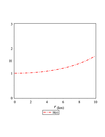
(a)  Metric potential H(r)

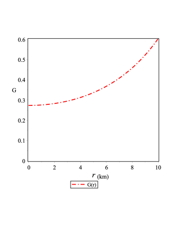
(b)  Metric potential G(r)

Figure 1: Schematic plots of the metric potentials (34) and (38) vs the radial coordinate $r$ in Km using the constants constrained by PSR J 1614–2230 data.

Density, radial and tangential pressures, given in Eq. (III), are plotted in Fig. 2.

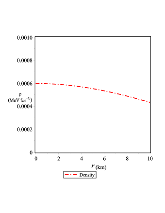
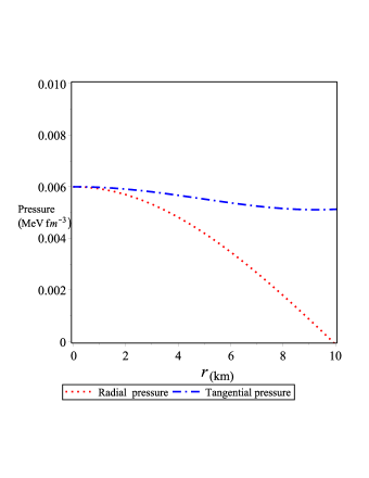
Figure 2: Plots of the density, radial and tangential pressures of (III) vs the radial coordinate $r$ in Km adopting PSR J 1614–2230 constraints. According to this, we assume the values of constants as $k\sim 28.248$, $c_{2}\sim 0.003$, $k_{1}\sim 0.492$.

Fig. 2 shows that density, radial and tangential pressures are positive as required for realistic stellar configuration. Moreover, as Fig. 2 2 shows, the density is high at the center and decreases far from it. Fig. 2 2 shows that the radial pressure goes to the zero at the boundary while the tangential pressure remains non-zero at the boundary. Also this feature is relevant for a realistic model.

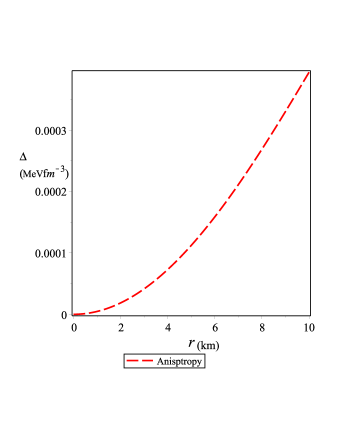
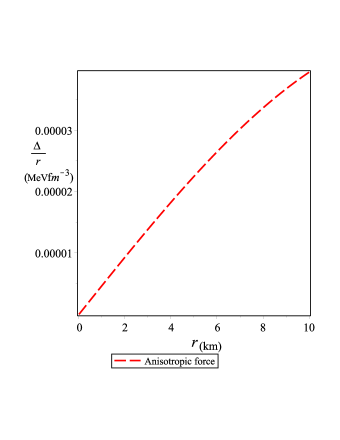
Figure 3: Plots of the anisotropy and anisotropic forces for solution (III) vs the radial coordinate $r$ in Km using PSR J 1614–2230 constraints.

Fig. 3 3 shows that the anisotropy is vanishing at the center and increases at the surface of the star. Specifically, Fig. 3 3 shows that the anisotropic force $\frac{\Delta}{r}$ is positive. This means that it is repulsive due to the fact that $p_{t}-p_{r}>0$.

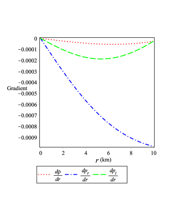
Figure 4: Plots of the density gradient, radial and tangential pressures of solution (III) versus the radial coordinate $r$ in Km using the PSR J 1614–2230 constraints.

Fig. 4 shows that the gradients of density, radial and tangential pressures are negative which confirms the decreasing of density, radial and transverse pressures through the stellar configuration.

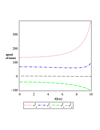
Figure 5: Plots of the radial and tangential sound speeds vs the radial coordinate $r$ in Km using the PSR J 1614–2230 constraints.

In Fig. 5, the radial and tangential speeds of sound are reported. They are positive and both of them are less than one. This result confirms the non-violations of causality condition in the interior of the star.

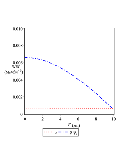
(a)  Weak energy conditions

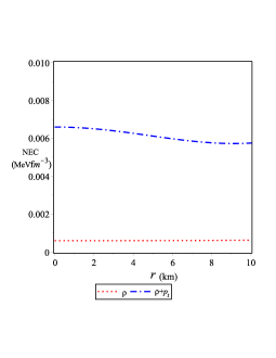
(b)  Null energy conditions

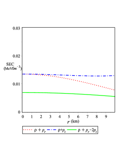
(c)  Strong energy condition

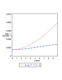
(d)  Dominant energy condition

Figure 6: Plots of the weak, null, strong and dominant energy conditions coming from (III) vs the radial coordinate $r$ in Km using the PSR J 1614–2230 constraints.

Fig. 6 represent the behavior of the energy conditions. In particular, Figs. 6 5(a), 5(b), 5(c) and 5(d) show the positive values of the WEC, NEC, SEC and DEC energy conditions. Therefore, all the energy conditions are satisfied throughout the stellar configuration as required for a physically meaningful stellar model.

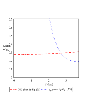
(a)  Matching condition of the potential G(R)

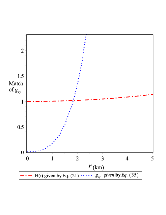
(b)  Matching condition of the potential H(R)

Figure 7: Plot of the radial coordinate $r$ in Km versus the weak, null, strong and dominant energy conditions from (III) using the constants constrained by PSR J 1614–2230 data.

The matching of the interior and exterior metrics at the boundary are shown in Fig. 7. Fig. 7 6(a) represents the smooth matching between $G(R)$ and $1-\frac{2M}{R}+\frac{Q^{2}}{R^{2}}$. Fig. 7 6(b) shows the smooth matching between $H(R)$ and $(1-\frac{2M}{R}+\frac{Q^{2}}{R^{2}})^{-1}$.

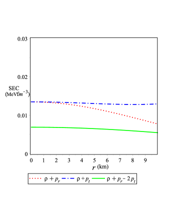
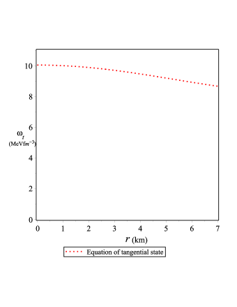
Figure 8: Plot of the density $\rho$ in $MeVfm^{3}$ versus the radial pressure $p_{r}$ and tangential pressure $p_{t}$ $MeVfm^{3}$, using the constants constrained by PSR J 1614–2230.

In Fig. 8, we have plotted radial and tangential EoS. As Fig 8 8, and 8 show, the EoS is not linear. In Ref. Das et al. (2019), authors derive the EoS for neutral compact stars and show that it is almost a linear one. Here, both the radial and tangential EoS show non-linear form which is due to the contribution of the electric field.

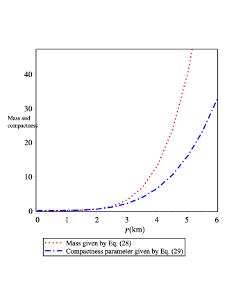
Figure 9: Plot of the Mass function vs the radius $r$ using the constants constrained by PSR J 1614–2230.

The mass function given by Eq. (44) is plotted in Fig. 9 which shows that it is a monotonically increasing function of the radial coordinate and $M(r=0)=0$. Moreover, Fig. 9 shows the behavior of the compactness parameter of star which is increasing.

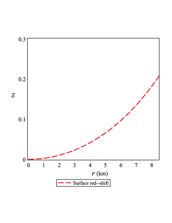
Figure 10: Plot of the surface red–shift versus the radius $r$ using the constants constrained by PSR J 1614–2230.

The radial variation of the surface red-shift is plotted in Fig. 10. Böhmer and Harko Böhmer and Harko (2006) constrained the surface red-shift to be $Z\leq 5$. The surface redshift of this model is calculated according to $PSRJ1614-2230$ and found to be $0.186927610$.

Using Eqs. (III) and (45), it is possible to derive the Mass-Radius $(M,R)$ relation of the model for a given value of the surface density $(\rho(r=R)=1.5\approx 10^{15}\frac{g}{cm^{3}})$. In Fig. 11, it is reported considering also the compactness–radius relation. As Fig. 11 10(c) shows, our model has a maximum mass 3$M_{\circledcirc}$ which is well beyond the recently reported values of 2.50-2.67$M_{\circledcirc}$ recently reported by the LIGO collaboration Abbott et al. (2020). This means that anomalous compact objects can be addressed in the framework of TEGR.

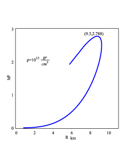
(a)  Mass–Radius with vanishing electromagnetic

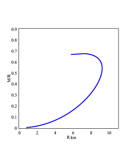
(b)  Compactness–Radius with vanishing electromagnetic

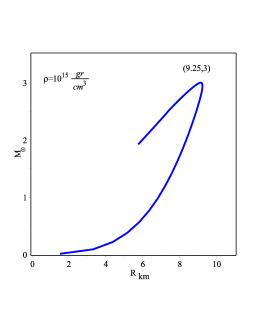
(c)  Mass–Radius with electromagnetic

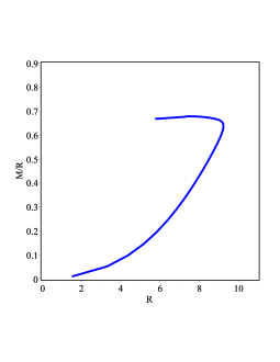
(d)  Compactness–Radius with electromagnetic

Figure 11: Plot of the Mass–Radius and compact–radius with/without electromagnetic field

VII Stability of the model

In this section we are going to discuss the stability issue using two different techniques; the Tolman-Oppenheimer-Volkoff equations and the adiabatic index.

VII.1 Equilibrium analysis through Tolman-Oppenheimer-Volkoff equation

In this subsection we are going to discuss the stability of the model. To this goal, we assume hydrostatic equilibrium through the Tolman-Oppenheimer-Volkoff (TOV) equation. Using the TOV equation Tolman (1939); Oppenheimer and Volkoff (1939) as that presented in Ponce de Leon (1993), we get the following form

$$\frac{2[p_{t}-p_{r}]}{r}-\frac{M_{g}(r)[\rho(r)+p_{r}]\sqrt{G}}{r\sqrt{H}}-\frac{dp_{r}}{r}+\sigma E\sqrt{H}=0,$$ (55)

with $M_{g}(r)$ being the gravitational mass at radius $r$, as defined by the Tolman-Whittaker mass formula which gives

$$M_{g}(r)=4\pi{\int_{0}}^{r}\Big{(}{T_{t}}^{t}-{T_{r}}^{r}-{T_{\theta}}^{\theta}-{T_{\phi}}^{\phi}\Big{)}r^{2}\sqrt{GH}dr=\frac{rG^{\prime}\sqrt{H}}{2G}\,,$$ (56)

Inserting Eq. (56) into (55), we get

$$\frac{2(p_{t}-p_{r})}{r}-\frac{dp_{r}}{dr}-\frac{G^{\prime}[\rho(r)+p_{r}]}{2\sqrt{G}}+\sigma E\sqrt{H}=F_{g}+F_{a}+F_{h}+F_{e}=0\,,$$ (57)

where $F_{g}=-\frac{G^{\prime}[\rho(r)+p_{r}]}{2{G}}$, $F_{a}=\frac{2(p_{t}-p_{r})}{r}$, $F_{h}=-\frac{dp_{r}}{dr}$ and $F_{e}=\sigma E\sqrt{H}$ are the gravitational, the anisotropic, the hydrostatic and the electromagnetic forces respectively. The behavior of the TOV equation for the model (III) is shown in Fig. 12.

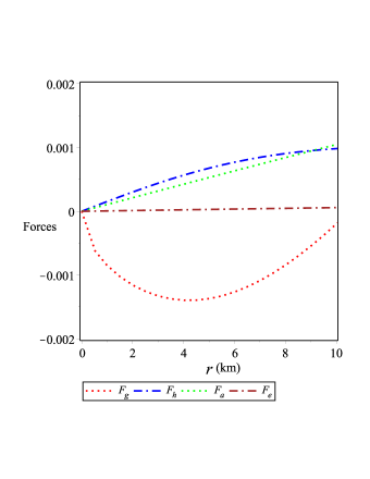
Figure 12: Plot of the gravitational, the anisotropic, the hydrostatic and the electromagnetic forces versus the radius $r$ using the constants constrained from PSR J 1614–2230.

The four different forces are plotted in Fig. 12. It shows that hydrostatics, anisotropic and electromagnetic forces are positive and dominated by the gravitational force which is negative to keep the system in static equilibrium.

VII.2 Stability in the static state

It was shown by Harrison, Zeldovich and Novikov Zeldovich and Novikov (1971, 1983) that, for stable compact stars, the gradient of central density, with regard to the mass increasing, must be positive, i.e., $\frac{\partial M}{\partial\rho_{{}_{r_{0}}}}>0$. If this condition is verified, we have stable configurations. Specifically, stable or unstable regions are separated when we have a constant mass i.e. $\frac{\partial M}{\partial\rho_{r_{0}}}=0$. Now we are going to apply this condition to our solution (III). For this purpose, we calculate the central density for solution (III) and get

$$\rho_{{}_{r_{0}}}=\frac{3}{2\pi k^{2}}\Rightarrow k=\pm\frac{\sqrt{3}}{\pi\sqrt{2\rho_{{}_{r_{0}}}}}\,.$$ (58)

Using Eq. (58) in Eq. (45), we get

$$M(\rho_{{}_{r_{0}}})=\frac{R^{3}(81R^{2}k_{1}{}^{2}+\pi[324k_{1}R^{2}+540\rho_{{}_{r_{0}}}-540\pi R^{2}\rho_{{}_{r_{0}}}{}^{2}+240\pi^{2}R^{4}\rho_{{}_{r_{0}}}{}^{3}-40\pi^{3}R^{4}\rho_{{}_{r_{0}}}{}^{4}])}{405}\,.$$ (59)

With the help of Eq. (59), we have

$$\frac{\partial M}{\partial\rho_{{}_{r_{0}}}}=\frac{\pi R^{3}(540-1080\pi R^{2}\rho_{{}_{r_{0}}}+720\pi^{2}R^{4}\rho_{{}_{r_{0}}}{}^{2}-160\pi^{3}R^{6}\rho_{{}_{r_{0}}}{}^{3})}{405}\,.$$ (60)

From Eq. (60), it is crear that solution (III) has a stable configuration since $\frac{\partial M}{\partial\rho_{r_{0}}}>0$. The behavior of (59) and (60) are show in Fig. 13. Fig. 13 shows that mass increases as the energy density increases and the mass gradient decreases as energy density increases.

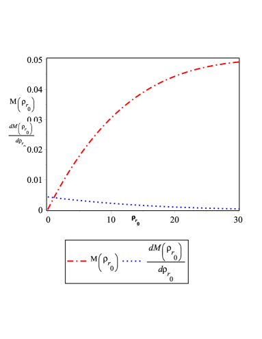
Figure 13: Static stability of (III) against $\rho_{r_{0}}$ in $\mathrm{km}^{-3}$ when $b_{0}=b_{2}=0.0001,R=0.1$.

VII.3 Adiabatic index

The stable equilibrium configuration of a spherically symmetric system can be studied using the adiabatic index which is a basic ingredient of the stability criterion. Let us consider an adiabatic perturbation, the adiabatic index $\Gamma$, is defined as Chandrasekhar (1964); Merafina and Ruffini (1989); Chan et al. (1993)

$$\Gamma=\left(\frac{\rho+p}{p}\right)\left(\frac{dp}{d\rho}\right)\,.$$ (61)

A Newtonian isotropic sphere is in stable equilibrium if the adiabatic index $\Gamma>\frac{4}{3}$ as reported in Heintzmann and Hillebrandth Heintzmann and Hillebrandt (1975). For $\Gamma=\frac{4}{3}$, the isotropic sphere is in neutral equilibrium. Based on some works by Chan et al. Chan et al. (1993), one can require the following condition for the stability of a relativistic anisotropic sphere $\Gamma>\gamma$ where

$$\gamma=\frac{4}{3}-\left\{\frac{4(p_{r}-p_{t})}{3\lvert p^{\prime}_{r}\lvert}\right\}_{max}\,.$$ (62)

Using Eq. (62), we get

$$\Gamma=\frac{4}{3}-\frac{2}{3}\Big{[}(c_{2}r^{2}+1)^{2}(4k_{1}{}^{2}k^{8}+6k^{4}-8r^{2}k^{2}+3r^{4})\Big{]}\times\Big{[}2(c_{2}r^{2}+1)^{2}k^{8}k_{1}{}^{2}+16k^{6}c_{2}-18c_{2}{}^{2}r^{4}k^{4}-36k^{4}c_{2}r^{2}+6k^{4}$$

$$+16c_{2}r^{4}k^{2}-16k^{2}r^{2}+16c_{2}{}^{2}r^{6}k^{2}+2c_{2}r^{6}+9r^{4}-3c_{2}{}^{2}r^{8}+4c_{2}{}^{2}k^{8}\Big{]}^{-1}.$$ (63)

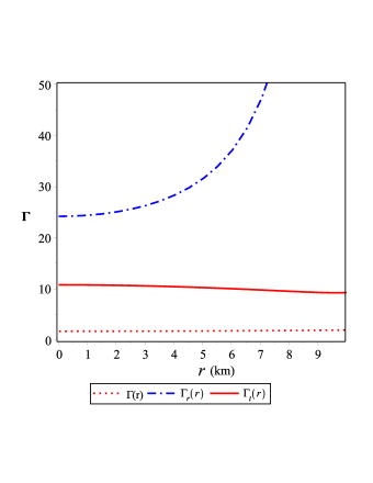
Figure 14: Plot of the adiabatic index versus the radius $r$ using the constants constrained from PSR J 1614–2230.

From Eq. (61), we obtain the adiabatic index of solution (III) in the form

$$\Gamma_{r}=\Big{\{}4(k^{2}-r^{2})^{3}(3+c_{2}[2r^{2}+k^{2}])\Big{[}2k^{8}(k_{1}{}^{2}\{1+c_{2}{}r^{2}\}^{2}+2c_{2}{}^{2})+16c_{2}k^{6}+6k^{4}(1-3c_{2}r^{2}[2+c_{2}r^{2}])$$

$$+16k^{2}r^{2}(c_{2}r^{2}-1+c_{2}{}^{2}r^{4})-3c_{2}{}^{2}r^{8}+2c_{2}r^{6}+9r^{4}\Big{]}\Big{\}}\Big{\{}[1+c_{2}r^{2}]^{2}\Big{[}2k^{8}(k_{1}{}^{2}r^{2}\{1+c_{2}r^{2}\}-2c_{2}{}^{2})+16c_{2}k^{6}r^{2}$$

$$+6k^{4}r^{2}[1-3c_{2}r^{2}]+8k^{2}r^{2}(c_{2}r^{2}-1)+3r^{6}-c_{2}r^{8}\Big{]}[2k^{8}k_{1}{}^{2}-30k^{4}+56k^{2}r^{2}-27r^{4}]\Big{\}}\,,$$

$$\Gamma_{t}=\Big{[}4k^{8}(k_{1}{}^{2}r^{2}\{1+c_{2}{}r^{2}\}+c_{2})+4k^{6}(3-c_{2}r^{2})-6k^{4}r^{2}(5+c_{2}r^{2})+4k^{2}r^{2}(3c_{2}r^{4}+7)-9r^{6}-5c_{2}r^{8}\Big{]}$$

$$\Big{[}k^{8}(k_{1}{}^{2}\{1+c_{2}r^{2}\}^{2}-2c_{2}{}^{2})-8c_{2}k^{6}+12c_{2}r^{2}k^{4}[c_{2}r^{2}+2]-8k^{2}r^{4}c_{2}[2c_{2}r^{2}+3]+2c_{2}r^{6}(4+3r^{2}c_{2})\Big{]}$$

$$\Big{\{}[1+c_{2}r^{2}]^{2}\Big{[}k^{8}(k_{1}{}^{2}r^{2}\{1+c_{2}r^{2}\}+2c_{2}{})-8c_{2}k^{6}r^{2}+12k^{4}r^{4}c_{2}-8k^{2}r^{6}c_{2}+2c_{2}r^{8}\Big{]}[2k^{8}k_{1}{}^{2}-30k^{4}+56k^{2}r^{2}-27r^{4}]\Big{\}}\,.$$

In Fig. 14 we have reported $\Gamma$, $\Gamma_{r}$ and $\Gamma_{t}$ respectively. As it is clear from these plots, it can be seen that the values of $\Gamma_{r}$ and $\Gamma_{t}$ are greater than $\Gamma$ throughout the stellar interior and hence the stability condition is fulfilled.

Table 1: Values of model parameters

Pulsar	Mass ($M_{\odot}$)	Radius (km)	k	$k_{1}$	$c_{1}$	$c_{2}$
Her X-1	$0.85\pm 0.15$	$8.1\pm 0.41$	33.43508140	0.8680552960$\times 10^{-2}$	450680.0914	0.5000000015$\times 10^{-2}$
Cen X-3	$1.49\pm 0.08$	$9.178\pm 0.13$	29.76976530	0.7072954467$\times 10^{-2}$	206264.0176	0.5000000001$\times 10^{-2}$
RX J 1856 -37	$0.9\pm 0.2$	$\simeq 6$	18.26492898	.1121853911$\times 10^{-1}$	40286.21339	0.5000000003$\times 10^{-2}$
4U1608 - 52	$1.74\pm 0.14$	$9.52\pm 0.15$	28.41404292	0.6372911235$\times 10^{-2}$	144607.5846	0.4999999996$\times 10^{-2}$
EXO 1785 - 248	$1.3\pm 0.2$	$8.849\pm 0.4$	28.50683773	0.6625295030$\times 10^{-2}$	269103.9598	0.3000000010$\times 10^{-2}$
4U1820 - 30	$1.58$	$9.1$	28.61239325	0.2556454675$\times 10^{-2}$	315783.9636	0.7000000014$\times 10^{-3}$

Table 2: Values of physical quantities

Pulsar	$\rho\lvert_{{}_{{}_{0}}}$	$\rho\lvert_{{}_{{}_{R}}}$	$\frac{dp_{r}}{d\rho}\lvert_{{}_{{}_{0}}}$	$\frac{dp_{r}}{d\rho}\lvert_{{}_{{}_{R}}}$	$\frac{dp_{t}}{d\rho}\lvert_{{}_{{}_{0}}}$	$\frac{dp_{t}}{d\rho}\lvert_{{}_{{}_{R}}}$	$(\rho-p_{r}-2p_{t})\lvert_{{}_{{}_{0}}}$	$(\rho-p_{r}-2p_{t})\lvert_{{}_{{}_{R}}}$	$z\lvert_{{}_{{}_{R}}}$
Her X-1	0.54$\times 10^{-2}$	.46$\times 10^{-2}$	.64	.60	.30	.25	.24$\times 10^{-2}$	.25$\times 10^{-2}$	.31
Cen X-3	0.68$\times 10^{-2}$	.53$\times 10^{-2}$	.50	.45	.24	.2	.38$\times 10^{-2}$	.37$\times 10^{-2}$	.51
RX J 1856 -37	.18$\times 10^{-1}$	.14$\times 10^{-1}$	.31	.28	.84$\times 10^{-1}$	.69$\times 10^{-1}$	.15$\times 10^{-1}$	.13$\times 10^{-1}$	.58
4U1608 - 52	.74$\times 10^{-2}$	.55$\times 10^{-2}$	.44	.37	.24	.2	.44$\times 10^{-2}$	.41$\times 10^{-2}$	.64
EXO 1785 - 248	.74$\times 10^{-2}$	.6$\times 10^{-2}$	.36	.34	.12	.10	.56$\times 10^{-2}$	.5$\times 10^{-2}$	.44
4U1820 - 30	.73$\times 10^{-2}$	.57$\times 10^{-2}$	.24	.21	.28$\times 10^{-1}$	.24$\times 10^{-1}$	.7$\times 10^{-2}$	.7$\times 10^{-2}$	.5

Besides PSR J 1614-2230, a similar analysis can be developed for other pulsars. In Table I and II, we report the results for other observed systems.

VIII Discussion and conclusions

An important remark is in order at this point. It is well known that TEGR theory is equivalent to GR up to a total derivative term Golovnev et al. (2017); Krššák et al. (2019); Bejarano et al. (2019). In this paper, we considered a combination of anisotropy and charge in TEGR equations. This situation gives rise to the effects of enhancing mass and modifying the $(M,R)$ relation of GR.

For a class of metric potentials and anisotropy functions, we derived an exact solution capable of figuring out realistic compact star configurations. The regularity conditions of the solution at the origin as well as at the surface of the star show a well behavior throughout the stellar structure. This is different from the results reported in Newton Singh et al. (2019) for GR. In that study, the authors show that pressure increases outward which is a non-physical situation. The difference between our results and those reported in Newton Singh et al. (2019) is due to the anisotropy given in Eq. (36), the presence of charge, and the non-vanishing of the radial pressure. In Newton Singh et al. (2019), they assumed a vanishing radial pressure. In our case, we showed that density, radial and tangential pressures behave regularly according to the observational data of the pulsar PSR J 1614–2230, the first reported very massive neutron star, whose existence ruled out many EoS Demorest et al. (2010). In order to explain such a system, exotic matter such as hyperons and kaon condensates, alternative theories of gravity and other hypotheses have been invoked (see e.g.Astashenok et al. (2015b, 2014, 2013)). The approach seems to work for other systems, as reported in Tables I and II.

Furthermore, we show that the anisotropy has a positive value which can be interpreted as a repulsive force. This fact is because the tangential pressure is greater than the radial pressure, i.e., $p_{t}>p_{r}$ Sunzu et al. (2019). The issue of stability is studied and we showed that the derived model is stable against the different forces (gravitational, hydrostatic, anisotropic and electromagnetic) acting on it. We also calculated the sound of speed and showed that it is consistent with realistic compact stars in contrast to the analogue charged models formulated in GR, where an imaginary sound speed is derived Newton Singh et al. (2019). Finally we calculated the adiabatic index of our model and showed that also it represents a realistic physical star. It is worth noticing that the adiabatic index presented in Newton Singh et al. (2019) has a negative value which is not consistent with realistic stellar models. This indicates, in a clear way, that our assumption of the metric potential (34) and the anisotropy form (36) are physical assumptions that makes the resulting stellar model consistent with real stellar objects.

We tested the model over a wide range of reported observed values of masses and radii of pulsars (Tables I and II). The conclusion is that the fit is good also in these cases. Finally, we drew the mass–radius relation and showed the effect of electric field on it.

It is shown that the electric charge plays a central role in improving the results compared with the neutral case. Among these improvements, we have:
i- In the neutral case, one gets a maximum mass as $2.788M_{\odot}$ while, in the charged case, the maximum mass becomes $3M_{\odot}$.
ii- In the neutral case, one get an increasing radial pressure as reported in Newton Singh et al. (2019) while in the charged case, one gets a decreasing one which describes a consistent compact star.
iii- In the neutral star, one gets an imaginary sound speed Newton Singh et al. (2019) while, in the charged case, we get a real physical sound speed as shown in Fig. 5.

The approach can be summarized as follows: we used a non-diagonal form of the tetrad field that gives a null value of the torsion as soon as the metric potentials approach to $1$. This is a necessary condition for any physical tetrad field as reported in various studies Ilijić and Sossich (2018); Abbas et al. (2015); Momeni et al. (2018); Abbas et al. (2015); Chanda et al. (2019); Debnath (2019); Ilijic and Sossich (2018).

We can conclude that the comparison of our exact solution with the physical parameters of pulsars gives indications that the model can realistically represent observed systems. Furthermore, the approach can be extended to a large class of metrics and anisotropies, if the above physical requirements are satisfied. However, a detailed confrontation with observational data is needed. This will be the argument of a forthcoming paper.

References

- Weyl (1918) H. Weyl, Sitzungsberichte der Königlich Preußischen Akademie der Wissenschaften (Berlin , 465 (1918).
- Einstein (2006) A. Einstein, “Neue möglichkeit für eine einheitliche feldtheorie von gravitation und elektrizität,” (John Wiley and Sons, Ltd, 2006) pp. 322–326, https://onlinelibrary.wiley.com/doi/pdf/10.1002/3527608958.ch37 .
- Mueller-Hoissen and Nitsch (1983) F. Mueller-Hoissen and J. Nitsch, Phys. Rev. D28, 718 (1983).
- Capozziello et al. (2014) S. Capozziello, D. J. Cirilo-Lombardo, and M. De Laurentis, Int. J. Geom. Meth. Mod. Phys. 11, 1450081 (2014), arXiv:1401.6555 [gr-qc] .
- O’Raifeartaigh (1997) L. O’Raifeartaigh, The dawning of gauge theory (Princeton Univ. Press, Princeton, NJ, USA, 1997).
- Blagojević and Hehl (2013) M. Blagojević and F. W. Hehl, eds., Gauge Theories of Gravitation (World Scientific, Singapore, 2013).
- Hayashi and Shirafuji (1979) K. Hayashi and T. Shirafuji, Phys. Rev. D 19, 3524 (1979).
- Maluf (2013) J. W. Maluf, Annalen der Physik 525, 339–357 (2013).
- Wu and Geng (2012) Y.-P. Wu and C.-Q. Geng, Physical Review D 86 (2012), 10.1103/physrevd.86.104058.
- Capozziello et al. (2020) S. Capozziello, M. Capriolo, and L. Caso, Eur. Phys. J. C80, 156 (2020), arXiv:1912.12469 [gr-qc] .
- Awad et al. (2018a) A. Awad, W. El Hanafy, G. G. L. Nashed, S. D. Odintsov, and V. K. Oikonomou, JCAP 1807, 026 (2018a), arXiv:1710.00682 [gr-qc] .
- Awad et al. (2017) A. M. Awad, S. Capozziello, and G. G. L. Nashed, JHEP 07, 136 (2017), arXiv:1706.01773 [gr-qc] .
- El Hanafy and Nashed (2016a) W. El Hanafy and G. G. L. Nashed, Astrophys. Space Sci. 361, 68 (2016a), arXiv:1507.07377 [gr-qc] .
- Li et al. (2011) B. Li, T. P. Sotiriou, and J. D. Barrow, Phys. Rev. D83, 064035 (2011), arXiv:1010.1041 [gr-qc] .
- Shirafuji and Nashed (1997) T. Shirafuji and G. G. L. Nashed, Prog. Theor. Phys. 98, 1355 (1997), arXiv:gr-qc/9711010 [gr-qc] .
- El Hanafy and Nashed (2016b) W. El Hanafy and G. G. L. Nashed, Astrophysics and Space Science 361 (2016b), 10.1007/s10509-016-2662-y.
- Nashed (2011) G. Nashed, Annalen der Physik 523, 450–458 (2011).
- Krššák (2017) M. Krššák, Eur. Phys. J. C77, 44 (2017), arXiv:1510.06676 [gr-qc] .
- Nashed (2003) G. G. L. Nashed, Chaos Solitons Fractals 15, 841 (2003), arXiv:gr-qc/0301008 [gr-qc] .
- Awad et al. (2018b) A. Awad, W. E. Hanafy, G. Nashed, S. Odintsov, and V. Oikonomou, Journal of Cosmology and Astroparticle Physics 2018, 026–026 (2018b).
- Bahamonde et al. (2015) S. Bahamonde, C. G. Böhmer, and M. Wright, Phys. Rev. D92, 104042 (2015), arXiv:1508.05120 [gr-qc] .
- Cai et al. (2016) Y.-F. Cai, S. Capozziello, M. De Laurentis, and E. N. Saridakis, Rept. Prog. Phys. 79, 106901 (2016), arXiv:1511.07586 [gr-qc] .
- Bogdanos et al. (2010) C. Bogdanos, S. Capozziello, M. De Laurentis, and S. Nesseris, Astropart. Phys. 34, 236 (2010), arXiv:0911.3094 [gr-qc] .
- Abedi and Capozziello (2018) H. Abedi and S. Capozziello, Eur. Phys. J. C78, 474 (2018), arXiv:1712.05933 [gr-qc] .
- Capozziello et al. (2019) S. Capozziello, M. Capriolo, and L. Caso, Int. J. Geom. Meth. Mod. Phys. 16, 1950047 (2019), arXiv:1812.11557 [gr-qc] .
- Schwarzschild (1916) K. Schwarzschild, Sitzungsber. Preuss. Akad. Wiss. Berlin (Math. Phys.) 1916, 189 (1916), arXiv:physics/9905030 [physics] .
- Lemaitre (1997) G. Lemaitre, Gen.Rel.Grav. 29, 641 (1997).
- Mak and Harko (2004a) M. K. Mak and T. Harko, Phys. Rev. D 70, 024010 (2004a).
- Mak and Harko (2004b) M. K. Mak and T. Harko, Int. J. Mod. Phys. D13, 149 (2004b), arXiv:gr-qc/0309069 [gr-qc] .
- Ruderman (1972) M. Ruderman, Ann. Rev. Astron. Astrophys. 10, 427 (1972).
- Canuto (1975) V. Canuto, araa 13, 335 (1975).
- Kippenhahn et al. (2013) R. Kippenhahn, A. Weigert, and A. Weiss, Stellar Structure and Evolution; 2nd ed., Astronomy and Astrophysics Library (Springer, Berlin, 2013).
- Tamta and Fuloria (2017) R. Tamta and P. Fuloria, Journal of Modern Physics 08, 1762 (2017).
- Astashenok et al. (2015a) A. V. Astashenok, S. Capozziello, and S. D. Odintsov, Astrophys. Space Sci. 355, 333 (2015a), arXiv:1405.6663 [gr-qc] .
- Herrera and Santos (1994) L. Herrera and N. O. Santos, Astrophys. J. 438, 308 (1994).
- Letelier (1980) P. S. Letelier, Phys. Rev. D 22, 807 (1980).
- Sawyer (1972) R. F. Sawyer, Phys. Rev. Lett. 29, 382 (1972).
- Usov (2004) V. V. Usov, Phys. Rev. D 70, 067301 (2004).
- Sokolov (1980) A. I. Sokolov, Soviet Journal of Experimental and Theoretical Physics 52, 575 (1980).
- Dev and Gleiser (2003) K. Dev and M. Gleiser, General Relativity and Gravitation 35, 1435 (2003).
- Dev and Gleiser (2002) K. Dev and M. Gleiser, General Relativity and Gravitation 34, 1793 (2002).
- Gleiser and Dev (2004) M. Gleiser and K. Dev, International Journal of Modern Physics D 13, 1389–1397 (2004).
- Ivanov (2010) B. V. Ivanov, International Journal of Theoretical Physics 49, 1236–1243 (2010).
- Schunck and Mielke (2003) F. E. Schunck and E. W. Mielke, Class. Quant. Grav. 20, R301 (2003), arXiv:0801.0307 [astro-ph] .
- Morris and Thorne (1988) M. S. Morris and K. S. Thorne, Am. J. Phys. 56, 395 (1988).
- Cattoen et al. (2005) C. Cattoen, T. Faber, and M. Visser, Class. Quant. Grav. 22, 4189 (2005), arXiv:gr-qc/0505137 [gr-qc] .
- DeBenedictis et al. (2006) A. DeBenedictis, D. Horvat, S. Ilijić, S. Kloster, and K. S. Viswanathan, Classical and Quantum Gravity 23, 2303–2316 (2006).
- De Falco et al. (2020) V. De Falco, E. Battista, S. Capozziello, and M. De Laurentis, (2020), arXiv:2004.14849 [gr-qc] .
- Bowers and Liang (1974) R. L. Bowers and E. P. T. Liang, Astrophys. J. 188, 657 (1974).
- Chan et al. (2003) R. Chan, M. F. A. da Silva, and J. F. Villas da Rocha, Int. J. Mod. Phys. D12, 347 (2003), arXiv:gr-qc/0209067 [gr-qc] .
- Herrera and Santos (1997) L. Herrera and N. O. Santos, Monthly Notices of the Royal Astronomical Society 287, 161 (1997), http://oup.prod.sis.lan/mnras/article-pdf/287/1/161/3165978/287-1-161.pdf .
- Heintzmann and Hillebrandt (1975) H. Heintzmann and W. Hillebrandt, aap 38, 51 (1975).
- Astashenok et al. (2015b) A. V. Astashenok, S. Capozziello, and S. D. Odintsov, JCAP 1501, 001 (2015b), arXiv:1408.3856 [gr-qc] .
- Astashenok et al. (2014) A. V. Astashenok, S. Capozziello, and S. D. Odintsov, Phys. Rev. D89, 103509 (2014), arXiv:1401.4546 [gr-qc] .
- Astashenok et al. (2013) A. V. Astashenok, S. Capozziello, and S. D. Odintsov, JCAP 1312, 040 (2013), arXiv:1309.1978 [gr-qc] .
- Capozziello et al. (2016) S. Capozziello, M. De Laurentis, R. Farinelli, and S. D. Odintsov, Phys. Rev. D93, 023501 (2016), arXiv:1509.04163 [gr-qc] .
- Feola et al. (2020) P. Feola, X. J. Forteza, S. Capozziello, R. Cianci, and S. Vignolo, Phys. Rev. D101, 044037 (2020), arXiv:1909.08847 [astro-ph.HE] .
- (58) “Anisotropic neutron star models: stability against radial and nonradial pulsations. [general relativity theory, newtonian approximation],” .
- Bayin (1982) S. m. c. i. m. c. Bayin, Phys. Rev. D 26, 1262 (1982).
- Krori et al. (1984) K. D. Krori, P. Borgohain, and R. Devi, Canadian Journal of Physics 62, 239 (1984).
- Bondi (1993) H. Bondi, mnras 262, 1088 (1993).
- Bondi (1999) H. Bondi, mnras 302, 337 (1999).
- Barreto (1993) W. Barreto, apss 201, 191 (1993).
- Barreto et al. (2007) W. Barreto, B. Rodríguez, L. Rosales, and O. Serrano, General Relativity and Gravitation 39, 23 (2007).
- Coley and Tupper (1994) A. A. Coley and B. O. J. Tupper, Classical and Quantum Gravity 11, 2553 (1994).
- Martinez et al. (1994) J. Martinez, D. Pavon, and L. A. Nunez, mnras 271, 463 (1994).
- Singh et al. (1995) T. Singh, G. P. Singh, and A. M. Helmi, Il Nuovo Cimento B (1971-1996) 110, 387 (1995).
- Hernández et al. (1999) H. Hernández, L. A. Núñez, and U. Percoco, Classical and Quantum Gravity 16, 871–896 (1999).
- Harko and Mak (2000) T. Harko and M. Mak, Journal of Mathematical Physics 41, 4752 (2000).
- Patel and Mehta (1995) L. K. Patel and N. P. Mehta, Australian Journal of Physics 48, 635 (1995).
- Lake (2004) K. Lake, Phys. Rev. Lett. 92, 051101 (2004).
- Böhmer and Harko (2006) C. G. Böhmer and T. Harko, Classical and Quantum Gravity 23, 6479 (2006).
- Boehmer and Harko (2007) C. G. Boehmer and T. Harko, Mon. Not. Roy. Astron. Soc. 379, 393 (2007), arXiv:0705.1756 [gr-qc] .
- Esculpi et al. (2007) M. Esculpi, M. Malaver, and E. Aloma, General Relativity and Gravitation 39, 633 (2007).
- Khadekar and Tade (2007) G. Khadekar and S. Tade, Astrophysics and Space Science 310, 41 (2007).
- Karmakar et al. (2007) S. Karmakar, S. Mukherjee, R. Sharma, and S. D. Maharaj, Pramana 68, 881 (2007).
- Abreu et al. (2007) H. Abreu, H. Hernández, and L. A. Núñez, Classical and Quantum Gravity 24, 4631 (2007).
- IVANOV (2010) B. V. IVANOV, International Journal of Modern Physics A 25, 3975–3991 (2010).
- Herrera et al. (2009) L. Herrera, G. Le Denmat, and N. O. Santos, Phys. Rev. D 79, 087505 (2009).
- Mak and Harko (2003) M. Mak and T. Harko, Proceedings of the Royal Society of London. Series A: Mathematical, Physical and Engineering Sciences 459, 393–408 (2003).
- Sharma and Mukherjee (2002) R. Sharma and S. Mukherjee, Modern Physics Letters A 17, 2535 (2002).
- Maharaj and Maartens (1989) S. D. Maharaj and R. Maartens, General Relativity and Gravitation 21, 899 (1989).
- Chaisi and Maharaj (2006) M. Chaisi and S. D. Maharaj, Pramana 66, 609 (2006).
- Herrera et al. (2008) L. Herrera, J. Ospino, and A. Di Prisco, Phys. Rev. D 77, 027502 (2008).
- Chaisi and Maharaj (2005) M. Chaisi and S. D. Maharaj, General Relativity and Gravitation 37, 1177 (2005).
- Gokhroo and Mehra (1994) M. K. Gokhroo and A. L. Mehra, General Relativity and Gravitation 26, 75 (1994).
- Lake (2009) K. Lake, Phys. Rev. D 80, 064039 (2009).
- V O et al. (2012) T. V O, B. S. Ratanpal, and V. Chackara, International Journal of Modern Physics D 14 (2012).
- Thomas and Ratanpal (2007) V. O. Thomas and B. S. Ratanpal, International Journal of Modern Physics D 16, 1479 (2007).
- Tikekar and Thomas (2005) R. Tikekar and V. O. Thomas, Pramana 64, 5 (2005).
- Thirukkanesh and Maharaj (2008a) S. Thirukkanesh and S. D. Maharaj, Classical and Quantum Gravity 25, 235001 (2008a).
- Thirukkanesh and Maharaj (2008b) S. Thirukkanesh and S. D. Maharaj, Classical and Quantum Gravity 25, 235001 (2008b).
- Sharma and Ratanpal (2013) R. Sharma and B. S. Ratanpal, Int. J. Mod. Phys. D22, 1350074 (2013), arXiv:1307.1439 [gr-qc] .
- Pandya et al. (2015) D. M. Pandya, V. O. Thomas, and R. Sharma, apss 356, 285 (2015), arXiv:1411.5674 [physics.gen-ph] .
- Bhar et al. (2015) P. Bhar, M. H. Murad, and N. Pant, Astrophysics and Space Science 359, 13 (2015).
- Bekenstein (1971) J. D. Bekenstein, Phys. Rev. D 4, 2185 (1971).
- Dionysiou (1985) D. D. Dionysiou, apss 111, 207 (1985).
- Ray et al. (2003) S. Ray, A. L. Espíndola, M. Malheiro, J. P. S. Lemos, and V. T. Zanchin, Phys. Rev. D 68, 084004 (2003).
- Ghezzi (2005) C. R. Ghezzi, Phys. Rev. D 72, 104017 (2005).
- Lasky and Lun (2007) P. D. Lasky and A. W. C. Lun, Phys. Rev. D 75, 104010 (2007).
- Negreiros et al. (2009) R. P. m. c. Negreiros, F. Weber, M. Malheiro, and V. Usov, Phys. Rev. D 80, 083006 (2009).
- Olson and Bailyn (1976) E. Olson and M. Bailyn, Phys. Rev. D 13, 2204 (1976).
- Demorest et al. (2010) P. Demorest, T. Pennucci, S. Ransom, M. Roberts, and J. Hessels, Nature 467, 1081 (2010), arXiv:1010.5788 [astro-ph.HE] .
- Plebański (1970) J. Plebański, Lectures on non-linear electrodynamics: an extended version of lectures given at the Niels Bohr Institute and NORDITA, Copenhagen, in October 1968 (NORDITA, 1970).
- Nashed (2006a) G. G. L. Nashed, Mod. Phys. Lett. A21, 2241 (2006a), arXiv:gr-qc/0401041 [gr-qc] .
- Krššák and Saridakis (2016) M. Krššák and E. N. Saridakis, Class. Quant. Grav. 33, 115009 (2016), arXiv:1510.08432 [gr-qc] .
- Bahamonde et al. (2019) S. Bahamonde, K. Flathmann, and C. Pfeifer, (2019), arXiv:1907.10858 [gr-qc] .
- Newton Singh et al. (2019) K. Newton Singh, F. Rahaman, and A. Banerjee, Phys. Rev. D 100, 084023 (2019), arXiv:1909.10882 [gr-qc] .
- Cooperstock and de la Cruz (1978) F. I. Cooperstock and V. de la Cruz, General Relativity and Gravitation 9, 835 (1978).
- Herrera and Ponce de Leon (1985) L. Herrera and J. Ponce de Leon, Journal of Mathematical Physics 26, 2302 (1985).
- Florides and Synge (1974) P. S. Florides and J. L. Synge, Proceedings of the Royal Society of London. A. Mathematical and Physical Sciences 337, 529 (1974), https://royalsocietypublishing.org/doi/pdf/10.1098/rspa.1974.0065 .
- Das et al. (2003) A. Das, A. DeBenedictis, and N. Tariq, Journal of Mathematical Physics 44, 5637 (2003).
- Herrera (1992) L. Herrera, Physics Letters A 165, 206 (1992).
- Zeldovich and Novikov (1971) Y. B. Zeldovich and I. D. Novikov, Relativistic astrophysics. Vol.1: Stars and relativity (1971).
- Nashed and Shirafuji (2007) G. G. Nashed and T. Shirafuji, Int. J. Mod. Phys. D 16, 65 (2007), arXiv:0704.3898 [gr-qc] .
- Nashed (2013) G. G. L. Nashed, Phys. Rev. D88, 104034 (2013), arXiv:1311.3131 [gr-qc] .
- Nashed (2006b) G. G. Nashed, Eur. Phys. J. C 48, 303 (2006b), arXiv:gr-qc/0607114 .
- Gangopadhyay et al. (2013) T. Gangopadhyay, S. Ray, X.-D. Li, J. Dey, and M. Dey, Mon. Not. Roy. Astron. Soc. 431, 3216 (2013), arXiv:1303.1956 [astro-ph.HE] .
- Das et al. (2019) S. Das, F. Rahaman, and L. Baskey, Eur. Phys. J. C79, 853 (2019).
- Abbott et al. (2020) R. Abbott et al. (LIGO Scientific, Virgo), Astrophys. J. Lett. 896, L44 (2020), arXiv:2006.12611 [astro-ph.HE] .
- Tolman (1939) R. C. Tolman, Phys. Rev. 55, 364 (1939).
- Oppenheimer and Volkoff (1939) J. R. Oppenheimer and G. M. Volkoff, Phys. Rev. 55, 374 (1939).
- Ponce de Leon (1993) J. Ponce de Leon, General Relativity and Gravitation 25, 1123 (1993).
- Zeldovich and Novikov (1983) Y. Zeldovich and I. Novikov, RELATIVISTIC ASTROPHYSICS. VOL. 2. THE STRUCTURE AND EVOLUTION OF THE UNIVERSE (1983).
- Chandrasekhar (1964) S. Chandrasekhar, Astrophys. J. 140, 417 (1964).
- Merafina and Ruffini (1989) M. Merafina and R. Ruffini, aap 221, 4 (1989).
- Chan et al. (1993) R. Chan, L. Herrera, and N. O. Santos, Monthly Notices of the Royal Astronomical Society 265, 533 (1993), http://oup.prod.sis.lan/mnras/article-pdf/265/3/533/3807712/mnras265-0533.pdf .
- Golovnev et al. (2017) A. Golovnev, T. Koivisto, and M. Sandstad, Classical and Quantum Gravity 34, 145013 (2017).
- Krššák et al. (2019) M. Krššák, R. J. van den Hoogen, J. G. Pereira, C. G. Böhmer, and A. A. Coley, Classical and Quantum Gravity 36, 183001 (2019).
- Bejarano et al. (2019) C. Bejarano, R. Ferraro, F. Fiorini, and M. J. Guzmán, Universe 5, 158 (2019).
- Sunzu et al. (2019) J. M. Sunzu, A. K. Mathias, and S. D. Maharaj, Journal of Astrophysics and Astronomy 40, 8 (2019).
- Ilijić and Sossich (2018) S. c. v. Ilijić and M. Sossich, Phys. Rev. D 98, 064047 (2018).
- Abbas et al. (2015) G. Abbas, A. Kanwal, and M. Zubair, Astrophys. Space Sci. 357, 109 (2015), arXiv:1501.05829 [physics.gen-ph] .
- Momeni et al. (2018) D. Momeni, G. Abbas, S. Qaisar, Z. Zaz, and R. Myrzakulov, Can. J. Phys. 96, 1295 (2018), arXiv:1611.03727 [gr-qc] .
- Abbas et al. (2015) G. Abbas, S. Qaisar, and A. Jawad, apss 359, 17 (2015), arXiv:1509.06711 [physics.gen-ph] .
- Chanda et al. (2019) A. Chanda, S. Dey, and B. C. Paul, Eur. Phys. J. C79, 502 (2019).
- Debnath (2019) U. Debnath, Eur. Phys. J. C79, 499 (2019), arXiv:1901.04303 [gr-qc] .
- Ilijic and Sossich (2018) S. Ilijic and M. Sossich, Phys. Rev. D98, 064047 (2018), arXiv:1807.03068 [gr-qc] .