Classification of simply-transitive
Levi non-degenerate hypersurfaces in ${\mathbb{C}}^{3}$

Abstract.

Holomorphically homogeneous CR real hypersurfaces $M^{3}\subset\mathbb{C}^{2}$ were classified by Élie Cartan in 1932. In the next dimension, we complete the classification of simply-transitive Levi non-degenerate hypersurfaces $M^{5}\subset\mathbb{C}^{3}$ using a novel Lie algebraic approach independent of any earlier classifications of abstract Lie algebras. Central to our approach is a new coordinate-free formula for the fundamental (complexified) quartic tensor. Our final result has a unique (Levi-indefinite) non-tubular model, for which we demonstrate geometric relations to planar equi-affine geometry.

1. Introduction

In general CR dimension $n\geqslant 1$, the classification of locally homogeneous real hypersurfaces $M^{2n+1}\subset\mathbb{C}^{n+1}$ (up to local biholomorphisms) is a vast, infinite problem. In 1932, Élie Cartan [4, 5] settled the $n=1$ case, and substantial efforts have been made over the last 20 years to complete the $n=2$ case, cf. [16, 17, 18, 11, 8]. Most recently, the remaining “simply-transitive Levi-nondegenerate” part of the classification was addressed in [14, 1, 2, 19] using normal form methods. The main goal of this article is to unify and complete this final study through a novel approach. Our Theorem 1.1 presents the final classification, which thereby concludes the $n=2$ case.

Local Lie groups are analytic, so homogeneous $M^{2n+1}\subset\mathbb{C}^{n+1}$ may be assumed from the outset to be real analytic ($\mathcal{C}^{\omega}$). By Lie’s infinitesimalization principle [15], the group $\operatorname{Hol}(M)$ of local biholomorphic transformations of $\mathbb{C}^{n+1}$ stabilizing $M$ is better viewed as the real Lie algebra:

$$\mathfrak{hol}(M)\,:=\,\Big{\{}X={\textstyle{\sum_{k=1}^{n+1}}}\,a_{k}(z)\,\tfrac{\partial}{\partial z_{k}}\colon\,\,\big{(}X+\overline{X}\big{)}\big{|}_{M}\,\,\text{is tangent to}\,\,M\Big{\}},$$ (1.1)

where $z=(z_{1},\dots,z_{n+1})$ are coordinates on $\mathbb{C}^{n+1}$, with the $a_{k}(z)$ being holomorphic. As Lie did [15], we will consider local Lie transformation (pseudo-)groups, and mainly deal with their Lie algebras of vector fields. Clearly, $M$ is (locally) homogeneous if and only if $\forall p\in M$, the evaluation map $\mathfrak{hol}(M)\to T_{p}M$ sending $X\mapsto(X+\overline{X})|_{p}$ is surjective. One calls a homogeneous $M$ simply-transitive if ${\rm dim}\,M={\rm dim}_{\mathbb{R}}\mathfrak{hol}(M)$, and multiply-transitive if ${\rm dim}\,M<{\rm dim}_{\mathbb{R}}\mathfrak{hol}(M)$.

Recall that $M^{2n+1}\subset\mathbb{C}^{n+1}$ is tubular (or is a ‘tube’) if there is a biholomorphism $M\cong{\mathcal{S}}^{n}\times i\,\mathbb{R}^{n+1}$, where ${\mathcal{S}}\subset\mathbb{R}^{n+1}$ is a real hypersurface (its ‘base’). If ${\mathcal{S}}=\{{\mathcal{F}}(x_{1},\ldots,x_{n+1})=0\}\subset\mathbb{R}^{n+1}$ is a real hypersurface with $d{\mathcal{F}}\neq 0$ on ${\mathcal{S}}$, its associated tube is $M_{\mathcal{S}}=\{{\mathcal{F}}\big{(}\operatorname{Re}z_{1},\dots,\operatorname{Re}z_{n+1}\big{)}=0\}\subset{\mathbb{C}}^{n+1}$. A tube $M_{\mathcal{S}}$ is Levi non-degenerate if and only if its base ${\mathcal{S}}$ has non-degenerate Hessian, and the signatures of the Levi form and Hessian agree. Clearly $i\,\partial_{z_{1}},\dots,i\,\partial_{z_{n+1}}\in\mathfrak{hol}(M_{\mathcal{S}})$. Furthermore, any real affine symmetry ${\mathbf{S}}=\big{(}A_{k\ell}\,x_{\ell}+b_{k}\big{)}\,\partial_{x_{k}}$ (summation assumed on $1\leq k,\ell\leq n+1$) of ${\mathcal{S}}$ has ‘complexification’ $X={\mathbf{S}}^{\operatorname{cr}}=\big{(}A_{k\ell}\,z_{\ell}+b_{k}\big{)}\,\partial_{z_{k}}$ in $\mathfrak{hol}(M_{\mathcal{S}})$. Thus, an affinely homogeneous base yields a holomorphically homogeneous tube.

1.1. Main result

Restrict now considerations to Levi non-degenerate hypersurfaces $M^{5}\subset\mathbb{C}^{3}$, i.e. $n=2$. The multiply-transitive case was tackled in [17, 18], which completed the majority of the classification, except the Levi-indefinite branch with ${\rm dim}\,\mathfrak{hol}(M)=6$. Recently, the entire multiply-transitive classification was settled in [8]. The simply-transitive case was addressed in [14, 1, 2, 19], where they employed normal form methods and Mubarakzyanov’s classification of 5-dimensional Lie algebras. In this article, we independently settle the entire simply-transitive classification using a novel Lie algebraic approach that does not depend on earlier classifications of abstract Lie algebras. Our main classification result is:

Theorem 1.1.

Any simply-transitive Levi non-degenerate hypersurface $M^{5}\subset\mathbb{C}^{3}$ is locally biholomorphic to precisely one of the following.

(1)  Either one hypersurface among the $6$ families of tubular hypersurfaces listed in Table 1 below, with corresponding $5$ generators of $\mathfrak{hol}(M)$.

(2)  Or the single nontubular exceptional model:

$$\operatorname{Im}(w)\,=\,\big{|}\operatorname{Im}(z_{2})-w\,\operatorname{Im}(z_{1})\big{|}^{2},$$ (1.2)

having indefinite Levi signature and the infinitesimal symmetries:

$$z_{1}\,\partial_{z_{1}}-z_{2}\,\partial_{z_{2}}-2w\,\partial_{w},\ \ \ \ \ z_{1}\,\partial_{z_{2}}+\partial_{w},\ \ \ \ \ z_{2}\,\partial_{z_{1}}-w^{2}\,\partial_{w},\ \ \ \ \ \partial_{z_{1}},\ \ \ \ \ \partial_{z_{2}},$$ (1.3)

with Lie algebra structure $\mathfrak{saff}(2,\mathbb{R}):=\mathfrak{sl}(2,\mathbb{R})\ltimes\mathbb{R}^{2}$, i.e. the planar equi-affine Lie algebra.

ℱ(Re(z1),Re(z2),Re(w))=0beyond i∂z1,i∂z2,i∂w Levi-definitecondition𝖳​1​u=x1α​x2βNon-degeneracy: ​α​β​(1−α−β)≠0Restriction: ​(α,β)≠(1,1),(−1,1),(1,−1)Redundancy: ​(α,β)∼(β,α)∼(1α,−βα)​z1​∂z1+α​w​∂w,z2​∂z2+β​w​∂wα​β​(1−α−β)>0𝖳​2​u=(x12+x22)α​exp⁡(β​arctan⁡(x2x1))Non-degeneracy: ​α≠12&(α,β)≠(0,0)Restriction: ​(α,β)≠(1,0)Redundancy: ​(α,β)∼(α,−β)​z1​∂z1+z2​∂z2+2​α​w​∂w,z2​∂z1−z1​∂z2−β​w​∂wα>12𝖳​3​u=x1​(α​ln⁡(x1)+ln⁡(x2))Non-degeneracy: ​α≠−1​z1​∂z1−α​z2​∂z2+w​∂w,z2​∂z2+z1​∂wα<−1𝖳​4​(u−x1​x2+x133)2=α​(x2−x122)3Non-degeneracy: ​α≠−89Restriction: ​α≠0​z1​∂z1+2​z2​∂z2+3​w​∂w,∂z1+z1​∂z2+z2​∂wα<−89𝖳​5​x1​u=x22+ϵ​x1αNon-degeneracy: ​α≠1,2Restriction: ​α≠0​z1​∂z1+α2​z2​∂z2+(α−1)​w​∂w,z1​∂z2+2​z2​∂wϵ​(α−1)​(α−2)>0𝖳​6x1​u=x22+ϵ​x12​ln⁡(x1)​z1​∂z1+z2​∂z2+(ϵ​z1+w)​∂w,z1​∂z2+2​z2​∂wϵ=+1missing-subexpressionmissing-subexpressionmissing-subexpressionmissing-subexpressionLabelAffinely simply-transitivefragmentsnon-degenerate real surface F(x1,x2,u)0 fragmentsF(Re(z1),Re(z2),Re(w))0fragmentsbeyond isubscript𝑧1,isubscript𝑧2,i𝑤 Levi-definiteconditionmissing-subexpressionmissing-subexpressionmissing-subexpressionmissing-subexpressionmissing-subexpressionmissing-subexpressionmissing-subexpressionmissing-subexpression𝖳1𝑢superscriptsubscript𝑥1𝛼superscriptsubscript𝑥2𝛽missing-subexpressionNon-degeneracy: 𝛼𝛽1𝛼𝛽0Restriction: 𝛼𝛽111111similar-toRedundancy: 𝛼𝛽𝛽𝛼similar-to1𝛼𝛽𝛼subscript𝑧1subscriptsubscript𝑧1𝛼𝑤subscript𝑤subscript𝑧2subscriptsubscript𝑧2𝛽𝑤subscript𝑤𝛼𝛽1𝛼𝛽0missing-subexpressionmissing-subexpressionmissing-subexpressionmissing-subexpression𝖳2𝑢superscriptsuperscriptsubscript𝑥12superscriptsubscript𝑥22𝛼𝛽subscript𝑥2subscript𝑥1missing-subexpressionNon-degeneracy: 𝛼12𝛼𝛽00Restriction: 𝛼𝛽10similar-toRedundancy: 𝛼𝛽𝛼𝛽subscript𝑧1subscriptsubscript𝑧1subscript𝑧2subscriptsubscript𝑧22𝛼𝑤subscript𝑤subscript𝑧2subscriptsubscript𝑧1subscript𝑧1subscriptsubscript𝑧2𝛽𝑤subscript𝑤𝛼12missing-subexpressionmissing-subexpressionmissing-subexpressionmissing-subexpression𝖳3𝑢subscript𝑥1𝛼subscript𝑥1subscript𝑥2missing-subexpressionNon-degeneracy: 𝛼1subscript𝑧1subscriptsubscript𝑧1𝛼subscript𝑧2subscriptsubscript𝑧2𝑤subscript𝑤subscript𝑧2subscriptsubscript𝑧2subscript𝑧1subscript𝑤𝛼1missing-subexpressionmissing-subexpressionmissing-subexpressionmissing-subexpression𝖳4superscript𝑢subscript𝑥1subscript𝑥2superscriptsubscript𝑥1332𝛼superscriptsubscript𝑥2superscriptsubscript𝑥1223missing-subexpressionNon-degeneracy: 𝛼89Restriction: 𝛼0subscript𝑧1subscriptsubscript𝑧12subscript𝑧2subscriptsubscript𝑧23𝑤subscript𝑤subscriptsubscript𝑧1subscript𝑧1subscriptsubscript𝑧2subscript𝑧2subscript𝑤𝛼89missing-subexpressionmissing-subexpressionmissing-subexpressionmissing-subexpression𝖳5subscript𝑥1𝑢superscriptsubscript𝑥22italic-ϵsuperscriptsubscript𝑥1𝛼missing-subexpressionNon-degeneracy: 𝛼12Restriction: 𝛼0subscript𝑧1subscriptsubscript𝑧1𝛼2subscript𝑧2subscriptsubscript𝑧2𝛼1𝑤subscript𝑤subscript𝑧1subscriptsubscript𝑧22subscript𝑧2subscript𝑤italic-ϵ𝛼1𝛼20missing-subexpressionmissing-subexpressionmissing-subexpressionmissing-subexpression𝖳6subscript𝑥1𝑢superscriptsubscript𝑥22italic-ϵsuperscriptsubscript𝑥12subscript𝑥1subscript𝑧1subscriptsubscript𝑧1subscript𝑧2subscriptsubscript𝑧2italic-ϵsubscript𝑧1𝑤subscript𝑤subscript𝑧1subscriptsubscript𝑧22subscript𝑧2subscript𝑤italic-ϵ1\begin{array}[]{|c|@{\,}c@{\,}|@{\,}l@{\,}|c|}\hline\cr\mbox{Label}&\begin{tabular}[]{c}Affinely simply-transitive\\ non-degenerate real surface ${\mathcal{F}}(x_{1},x_{2},u)=0$\end{tabular}&\begin{tabular}[]{c}\rule[0.0pt]{0.0pt}{11.0pt} Holomorphic symmetries of\\ ${\mathcal{F}}(\operatorname{Re}(z_{1}),\operatorname{Re}(z_{2}),\operatorname{Re}(w))=0$\\ beyond $i\partial_{z_{1}},i\partial_{z_{2}},i\partial_{w}$ \rule[-5.0pt]{0.0pt}{11.0pt}\end{tabular}&\begin{tabular}[]{c}Levi-definite\\ condition\\ \end{tabular}\\ \hline\cr\hline\cr\mathsf{T}1&\begin{array}[]{c}\rule[0.0pt]{0.0pt}{10.0pt}u=x_{1}^{\alpha}x_{2}^{\beta}\\ \\ \mbox{\scriptsize Non-degeneracy: }\alpha\beta(1-\alpha-\beta)\neq 0\\ \mbox{\scriptsize Restriction: }(\alpha,\beta)\neq(1,1),(-1,1),(1,-1)\\ \mbox{\scriptsize Redundancy: }(\alpha,\beta)\sim(\beta,\alpha)\sim\left(\frac{1}{\alpha},-\frac{\beta}{\alpha}\right)\rule[-6.0pt]{0.0pt}{11.0pt}\end{array}&\begin{array}[]{l}z_{1}\partial_{z_{1}}+\alpha w\partial_{w},\\ z_{2}\partial_{z_{2}}+\beta w\partial_{w}\end{array}&\alpha\beta(1-\alpha-\beta)>0\\ \hline\cr\mathsf{T}2&\begin{array}[]{c}\rule[0.0pt]{0.0pt}{11.0pt}u=\left(x_{1}^{2}+x_{2}^{2}\right)^{\alpha}\exp\big{(}\beta\arctan(\frac{x_{2}}{x_{1}})\big{)}\\ \\ \mbox{\scriptsize Non-degeneracy: }\alpha\neq\frac{1}{2}\,\,\&\,\,(\alpha,\beta)\neq(0,0)\\ \mbox{\scriptsize Restriction: }(\alpha,\beta)\neq(1,0)\\ \mbox{\scriptsize Redundancy: }(\alpha,\beta)\sim(\alpha,-\beta)\rule[-5.0pt]{0.0pt}{11.0pt}\end{array}&\begin{array}[]{l}z_{1}\partial_{z_{1}}+z_{2}\partial_{z_{2}}+2\alpha w\partial_{w},\\ z_{2}\partial_{z_{1}}-z_{1}\partial_{z_{2}}-\beta w\partial_{w}\end{array}&\alpha>\frac{1}{2}\\ \hline\cr\mathsf{T}3&\begin{array}[]{c}\rule[0.0pt]{0.0pt}{11.0pt}u=x_{1}\left(\alpha\ln(x_{1})+\ln(x_{2})\right)\\ \\ \mbox{\scriptsize Non-degeneracy: }\alpha\neq-1\rule[-4.0pt]{0.0pt}{11.0pt}\end{array}&\begin{array}[]{l}z_{1}\partial_{z_{1}}-\alpha z_{2}\partial_{z_{2}}+w\partial_{w},\\ z_{2}\partial_{z_{2}}+z_{1}\partial_{w}\end{array}&\alpha<-1\\ \hline\cr\mathsf{T}4&\begin{array}[]{c}\rule[0.0pt]{0.0pt}{12.0pt}\big{(}u-x_{1}x_{2}+\frac{x_{1}^{3}}{3}\big{)}^{2}=\alpha\big{(}x_{2}-\frac{x_{1}^{2}}{2}\big{)}^{3}\\ \\ \mbox{\scriptsize Non-degeneracy: }\alpha\neq-\frac{8}{9}\\ \mbox{\scriptsize Restriction: }\alpha\neq 0\rule[-4.0pt]{0.0pt}{11.0pt}\end{array}&\begin{array}[]{l}z_{1}\partial_{z_{1}}+2z_{2}\partial_{z_{2}}+3w\partial_{w},\\ \partial_{z_{1}}+z_{1}\partial_{z_{2}}+z_{2}\partial_{w}\end{array}&\alpha<-\frac{8}{9}\\ \hline\cr\mathsf{T}5&\begin{array}[]{c}\rule[0.0pt]{0.0pt}{11.0pt}x_{1}u=x_{2}^{2}+\epsilon x_{1}^{\alpha}\\ \\ \mbox{\scriptsize Non-degeneracy: }\alpha\neq 1,2\\ \mbox{\scriptsize Restriction: }\alpha\neq 0\rule[-4.0pt]{0.0pt}{11.0pt}\end{array}&\begin{array}[]{l}z_{1}\partial_{z_{1}}+\frac{\alpha}{2}z_{2}\partial_{z_{2}}+(\alpha-1)w\partial_{w},\\ z_{1}\partial_{z_{2}}+2z_{2}\partial_{w}\end{array}&\epsilon(\alpha-1)(\alpha-2)>0\\ \hline\cr\mathsf{T}6&\begin{array}[]{c}x_{1}u=x_{2}^{2}+\epsilon x_{1}^{2}\ln(x_{1})\\ \end{array}&\begin{array}[]{l}\rule[0.0pt]{0.0pt}{10.0pt}z_{1}\partial_{z_{1}}+z_{2}\partial_{z_{2}}+(\epsilon z_{1}+w)\partial_{w},\\ z_{1}\partial_{z_{2}}+2z_{2}\partial_{w}\rule[-5.0pt]{0.0pt}{11.0pt}\end{array}&\epsilon=+1\\ \hline\cr\end{array}

Holomorphic symmetries of Holomorphic symmetries of

Table 1. All simply-transitive tubes $M^{5}\subset\mathbb{C}^{3}$. Parameters $\alpha,\beta\in\mathbb{R}$ and $\epsilon=\pm 1$.

We immediately recover that all simply-transitive Levi-definite $M^{5}\subset\mathbb{C}^{3}$ are tubular [14].

The classification of affinely homogeneous surfaces ${\mathcal{S}}\subset\mathbb{R}^{3}$ appears in [6, 9]. A tube $M_{\mathcal{S}}$ on an affinely multiply-transitive base ${\mathcal{S}}$ is holomorphically multiply-transitive, so for the Levi non-degenerate simply-transitive tube classification, we can start from the DKR list [6] and perform the following:

1. Remove those surfaces yielding tubes already appearing in the multiply-transitive classification [8]. (See our Table 2 and Remark 6.6 in §6.2.)

2. Restrict to affinely simply-transitive surfaces that have non-degenerate Hessians. (This excludes all quadrics, cylinders, and the Cayley surface $u=x_{1}x_{2}-\frac{x_{1}^{3}}{3}$, cf. [6, Prop. in §3].)

The desired classification is a subset of the resulting candidate list, which comprises the surfaces in the 2nd column of Table 1. The symmetries in the 3rd column confirm that these all have ${\rm dim}\,\mathfrak{hol}(M)\geq 5$, but it is important to carefully identify all exceptions for which this dimension jumps up. Theorem 1.1 asserts that no such exceptions occur among the candidate list.

A comparison with the simply-transitive list in [19, Table 7, p. 50] is in order. The tubular classification there mostly matches ours, but differs in the $\mathsf{T}3$ and $\mathsf{T}4$ cases in our Table 1. For the former, $\alpha=0$ is incorrectly omitted; for the latter, the restriction should be corrected to $\alpha\neq 0,-\frac{8}{9}$. Moreover, two nontubular models are listed:

1. $(v-x_{2}y_{1})^{2}+y_{1}^{2}y_{2}^{2}=y_{1}$, which is equivalent to (1.2) – see §5.3. We moreover derive (1.2) in an elementary manner and elucidate some related planar equi-affine geometry.

2. $v(1+\epsilon x_{2}y_{2})=y_{1}y_{2}$ with $\epsilon=\pm 1$, which is Levi-degenerate at the origin and Levi-indefinite. We confirm that ${\rm dim}\,\mathfrak{hol}(M)=5$, with generators

   $$\big{(}2\,i+\epsilon\,z_{2}^{2}\big{)}\,\partial_{z_{1}}+2\,z_{2}\,\partial_{w},\ \ \ \ \ \epsilon\,w\,\partial_{z_{1}}+\partial_{z_{2}},\ \ \ \ \ z_{1}\,\partial_{z_{1}}+w\,\partial_{w},\ \ \ \ \ \partial_{z_{1}},\ \ \ \ \ \partial_{w}.$$ (1.4)

   From the hypersurface equation, $y_{2}=\operatorname{Im}(z_{2})$ is locally unrestricted, but its level sets are clearly preserved by all symmetries (1.4), so this model is not homogeneous.

More broadly, Theorem 1.1 also terminates the problem of classifying all holomorphically homogeneous CR real hypersurfaces $M^{5}\subset{\mathbb{C}}^{3}$, as follows:

1. holomorphically degenerate: either the Levi-flat hyperplane $\mathbb{R}\times\mathbb{C}\times\mathbb{C}$, or ${\mathcal{M}}^{3}\times\mathbb{C}$ for some homogeneous Levi non-degenerate hypersurface ${\mathcal{M}}^{3}\subset\mathbb{C}^{2}$, classified by Cartan  [4, 5]. These all have ${\rm dim}\,\mathfrak{hol}(M)=\infty$.

2. holomorphically non-degenerate: From [21], there are two possibilities:

   1. constant Levi rank 1 and 2-nondegenerate: The classification was completed by Fels–Kaup in [11]. All such models are tubular, with ${\rm dim}\,\mathfrak{hol}(M)\leq 10$, which is sharp on the tube with base the future light cone ${\mathcal{S}}=\{x\in\mathbb{R}^{3}:x_{1}^{2}+x_{2}^{2}=x_{3}^{2},\,x_{3}>0\}$.

   2. Levi non-degenerate: ${\rm dim}\,\mathfrak{hol}(M)\leq 15$, which is sharp on the flat model $\operatorname{Im}\,w=|z_{1}|^{2}+\epsilon|z_{2}|^{2}$, where $\epsilon=\pm 1$. The biholomorphism $(z_{1},z_{2},w)\mapsto(z_{1},z_{2},i(2w-z_{1}^{2}-\epsilon z_{2}^{2}))$ maps this to the tube over $u=x_{1}^{2}+\epsilon x_{2}^{2}$.

1.2. Classification approach and further results

Some recent classification approaches focus on effective use of normal forms. For instance, in the simply-transitive, Levi-definite case [14], the authors realize 5-dimensional real Lie algebras acting transitively on real hypersurfaces by holomorphic vector fields and then find appropriate normal forms for such realizations. Their starting point is the classification of abstract 5-dimensional real Lie algebras (Mubarakzyanov [23]), but they also use an important discarding sieve: If $\mathfrak{hol}(M)$ is 5-dimensional and contains a 3-dimensional abelian ideal, then $M$ is tubular over an affinely homogeneous base [14, Prop.3.1]. In the end, no nontubular models survive and they invoke the DKR classification [6] for tubular cases.

Remark 1.2.

By our Theorem 1.1, we can a posteriori assert that [14, Prop.3.1], valid for a Lie algebra ${\mathfrak{g}}$ of holomorphic vector fields acting locally simply transitively on Levi-definite $M^{5}\subset{\mathbb{C}}^{3}$, also holds in the Levi-indefinite case. However, their proof does not carry over: it relies on [14, Prop.2.3], which states that if $X,Y,Z\in{\mathfrak{g}}$ commute and are linearly independent over ${\mathbb{R}}$ at $q\in M$, then $X,Y,Z$ are linearly independent over ${\mathbb{C}}$ at $q$. This may fail in the indefinite setting, as the following counterexample shows. Consider a hypersurface of Winkelmann type [8] given by $\operatorname{Im}(w+\overline{z}_{1}z_{2})=(z_{1})^{\alpha}(\overline{z}_{1})^{\overline{\alpha}}$ for $\alpha\in\mathbb{C}\backslash\{-1,0,1,2\}$, which is tubular if and only if $\frac{(2\alpha-1)^{2}}{(\alpha+1)(\alpha-2)}\in\mathbb{R}$. Then $\mathfrak{hol}(M)$ contains the abelian subalgebra

$$X_{1}=z_{1}\partial_{z_{2}},\quad X_{2}=\partial_{z_{2}}+z_{1}\partial_{w},\quad X_{3}=i\partial_{z_{2}}-iz_{1}\partial_{w},\quad X_{4}=\partial_{w}.$$ (1.5)

Evaluating at a point where $z_{1}\neq 0$, we see that $\{X_{1},X_{2},X_{3}\}$ are linearly independent over $\mathbb{R}$, but they are linearly dependent over $\mathbb{C}$.

Our approach to the non-tubular, simply-transitive classification is substantially different. Our approach circumvents the use of normal forms, is independent of the Mubarakzyanov classification, and draws upon the known close geometric relationship with so-called Legendrian contact structures that was similarly effectively used in [7, 8]. (The Cartan-geometric approach [7] in the simply-transitive setting would result in heavy case-branching, so this will not be used.) To describe our strategy, we need to recall some notions.

Any Levi non-degenerate hypersurface $M^{2n+1}\subset\mathbb{C}^{n}$ naturally inherits a CR structure of codimension 1, i.e. a contact distribution $C=TM\cap J(TM)\subset TM$ with a complex structure $J:C\to C$ compatible with the natural (conformal) symplectic form on $C$. The induced $J$ on the complexification $C^{\mathbb{C}}$ has $\pm i$ eigenspaces yielding isotropic, integrable subdistributions. Abstract CR structures $(M;C,J)$ (for which integrability is not required) have corresponding complexified analogues called Legendrian contact (LC) structures $(N;E,F)$. This consists of a complex contact manifold $(N^{2n+1},C)$ with the contact distribution $C$ split (instead of $C^{\mathbb{C}}$) into a pair of isotropic subdistributions $E$ and $F$ of equal dimension. It is an integrable (ILC) structure if both $E$ and $F$ are integrable.

Concretely, if $M^{2n+1}\subset\mathbb{C}^{n+1}$ has defining equation $\Phi(z,\overline{z})=0$, where $\Phi$ is real analytic, then we define its complexification $M^{c}\subset\mathbb{C}^{n+1}\times\mathbb{C}^{n+1}$ by $\Phi(z,a)=0$. (We can recover $M$ as the fixed-point set of the anti-involution $(z,a)\mapsto(\overline{a},\overline{z})$ restricted to $M^{c}$.) The associated double fibration

(1.10)

defined by $\pi_{1}(z,a)=z$ and $\pi_{2}(z,a)=a$ for $(z,a)\in M^{c}$, induces vertical (hence integrable) subdistributions $F=\ker(d\pi_{1})$ and $E=\ker(d\pi_{2})$ on $M^{c}$. Levi non-degeneracy of $M$ implies that $C=E\oplus F$ is a contact distribution on $M^{c}$, and indeed $(M^{c};E,F)$ is an ILC structure. Regarding $a\in\mathbb{C}^{n+1}$ as parameters, we view $M^{c}=\{\Phi(z,a)=0\}$ as describing a parametrized family of hypersurfaces in $\mathbb{C}^{n+1}$. These Segre varieties were introduced by Segre [26, 27], further explored by Cartan [4] in the $\mathbb{C}^{2}$ case, and extended more generally – see for example [28, 29, 20, 21, 8].

Locally solving $\Phi(z,a)=0$ for one variable among $z=(z_{1},\ldots,z_{n+1})$, say $w:=z_{n+1}$, then differentiating once, we can locally resolve all parameters $a$ in terms of the 1-jet $(z_{k},w,w_{\ell}:=\frac{\partial w}{\partial z_{\ell}})$ for $1\leq k,\ell\leq n$. Hence, we can differentiate one more time, eliminate parameters $a$, and write second partials as a complete 2nd order PDE system (considered up to local point transformations):

$$\frac{\partial^{2}w}{\partial z_{i}\partial z_{j}}=f_{ij}(z_{k},w,w_{\ell}).$$ (1.11)

The Segre varieties are now interpreted as the space of solutions of (1.11). (See (2.1) for $E$ and $F$.)

The symmetry algebra of an LC structure consists of all vector fields respectively preserving $E$ and $F$ under the Lie derivative. In terms of $M^{c}=\{\Phi(z,a)=0\}$, any symmetry is of the form $X=\xi^{k}(z)\partial_{z_{k}}+\sigma^{k}(a)\partial_{a_{k}}$. For example, given a tube $M_{\mathcal{S}}=\{{\mathcal{F}}(\operatorname{Re}z)=0\}$, its complexification $M_{\mathcal{S}}^{c}=\{{\mathcal{F}}(\frac{z+a}{2})=0\}$ admits the $(n+1)$-dimensional abelian subalgebra ${\mathfrak{a}}=\langle\partial_{z_{1}}-\partial_{a_{1}},\ldots,\partial_{z_{n+1}}-\partial_{a_{n+1}}\rangle$ that is clearly transverse to $E$ and $F$. In the PDE picture, any symmetry of (1.11) is projectable over the $(z_{k},w)$-space, and these are called point symmetries. For Levi non-degenerate $M\subset\mathbb{C}^{n+1}$, the symmetry algebra $\operatorname{sym}(M^{c})$ of the associated ILC structure $(M^{c};E,F)$ is simply $\mathfrak{hol}(M)\otimes_{\mathbb{R}}\mathbb{C}$, see [20, Cor. 6.36]. In particular,

$${\rm dim}_{\mathbb{C}}\operatorname{sym}(M^{c})={\rm dim}_{\mathbb{R}}\mathfrak{hol}(M).$$ (1.12)

For our simply-transitive study, $M$ or $M^{c}$ will be (locally) real or complex Lie groups respectively, and we encode data on their Lie algebras. Our focus will be on ASD-ILC triples:

Definition 1.3.

Let ${\mathfrak{g}}$ be a 5-dimensional complex Lie algebra. An ILC triple $({\mathfrak{g}};{\mathfrak{e}},{\mathfrak{f}})$ consists of a pair of 2-dimensional subalgebras ${\mathfrak{e}},{\mathfrak{f}}$ of ${\mathfrak{g}}$ with ${\mathfrak{e}}\cap{\mathfrak{f}}=0$ such that for $C:={\mathfrak{e}}\oplus{\mathfrak{f}}$, the map $\eta:\bigwedge^{2}C\to{\mathfrak{g}}/C$ given by $(x,y)\mapsto[x,y]\,{\rm mod}\ C$ is non-degenerate. An ILC triple is:

1. tubular if there exists a 3-dimensional subalgebra ${\mathfrak{a}}\subset{\mathfrak{g}}$ with ${\mathfrak{e}}\cap{\mathfrak{a}}={\mathfrak{f}}\cap{\mathfrak{a}}=0$;

2. anti-self-dual (ASD) if there exists an anti-involution $\tau$ of ${\mathfrak{g}}$ that swaps ${\mathfrak{e}}$ and ${\mathfrak{f}}$. In this case, call $\tau$ admissible. In the tubular case, $\tau$ is also required to stabilize ${\mathfrak{a}}$ above.

Given an ASD-ILC triple $({\mathfrak{g}};{\mathfrak{e}},{\mathfrak{f}})$, the fixed-point set of an admissible anti-involution $\tau$ determines the corresponding Lie algebraic CR data (and conversely). Letting $G$ be a (complex) Lie group with Lie algebra ${\mathfrak{g}}$, and $E,F$ determined from ${\mathfrak{e}},{\mathfrak{f}}$ by left translations in $G$, the ILC structure $(G;E,F)$ certainly has ILC symmetry dimension, denoted ${\rm dim}\operatorname{sym}_{\mathsf{ILC}}({\mathfrak{g}};{\mathfrak{e}},{\mathfrak{f}})$, at least ${\rm dim}\,G=5$. It is important to recognize and discard cases where it exceeds this. This occurs when there is an embedding (Definition 2.11) into an ILC quadruple $(\tilde{\mathfrak{g}},\tilde{\mathfrak{k}};\tilde{\mathfrak{e}},\tilde{\mathfrak{f}})$ with ${\rm dim}(\tilde{\mathfrak{k}})>0$. An important tool in this study is the fundamental quartic tensor ${\mathcal{Q}}_{4}$, which we now present.

For any (integrable) CR or ILC structure, it is well-known that there is a fundamental tensor that obstructs local equivalence to the flat model, which uniquely realizes the maximal symmetry dimension. When $n=2$, this tensor takes the form of a binary quartic ${\mathcal{Q}}_{4}$, and symmetry upper bounds based on its root type are known – see (2.20). In the CR setting, ${\mathcal{Q}}_{4}$ is typically computed from the fourth degree part of the Chern–Moser normal form [10], while in the SILC setting [7] it was computed in terms of a PDE realization (1.11). However, neither of these methods are amenable to a Lie algebraic approach. In §2, we give a coordinate-free formula for ${\mathcal{Q}}_{4}$ for general LC structures, which can be directly used on Lie algebraic data – in particular on an ASD-ILC triple $({\mathfrak{g}};{\mathfrak{e}},{\mathfrak{f}})$.

Our Lie algebraic study is organized in terms of 3-dimensional abelian ideals. In §3, we efficiently classify all 5-dimensional complex Lie algebras without a 3-dimensional abelian ideal (Proposition 3.2). The search for ASD-ILC triples supported on this small list of Lie algebras produces a unique model on ${\mathfrak{g}}=\mathfrak{saff}(2,\mathbb{C}):=\mathfrak{sl}(2,\mathbb{C})\ltimes\mathbb{C}^{2}$, see Theorem 3.1.

In §4, we study ASD-ILC triples $({\mathfrak{g}};{\mathfrak{e}},{\mathfrak{f}})$ with ${\mathfrak{g}}$ containing a 3-dimensional abelian ideal ${\mathfrak{a}}$. Theorem 4.1 shows that if ${\rm dim}\,\operatorname{sym}_{\mathsf{ILC}}({\mathfrak{g}};{\mathfrak{e}},{\mathfrak{f}})=5$, then ${\mathfrak{e}}\cap{\mathfrak{a}}={\mathfrak{f}}\cap{\mathfrak{a}}=0$ and ${\mathfrak{a}}=\tau({\mathfrak{a}})$ under any admissible anti-involution $\tau$. These data allow us to a priori conclude (Corollary 6.4) that all models in this branch are tubes on an affinely simply-transitive base.

We then return to CR geometry. In §5, we construct the exceptional model (1.2), highlight related planar equi-affine geometry, and find corresponding PDE realizations. Finally in §6, we treat the tubes for any candidate base arising from the DKR classification. Table 3 summarizes the root types for these tubes, which are deduced from the quartics ${\mathcal{Q}}_{4}$ given in Table 3. From (2.20), when the root type is $\mathsf{I}$ or $\mathsf{II}$, the symmetry dimension upper bound is 5, and such models are automatically simply-transitive. The root type $\mathsf{D}$ and $\mathsf{N}$ cases are more subtle, and simple-transitivity in these remaining cases are confirmed using two methods: PDE point symmetries (§6.3) and power series (§6.4).

Beyond our main result, let us emphasize two important results obtained in this article:

• We give a simple geometric interpretation and coordinate-free formula for the fundamental quartic tensor ${\mathcal{Q}}_{4}$ for general 5-dimensional LC structures.

• We conceptualize and give an effective method for computing symmetries of rigid CR structures, which potentially can be generalized to a much larger class of geometric structures.

2. Fundamental tensor of 5-dimensional Legendrian contact structures

Motivated by the complexification $M^{c}\subset\mathbb{C}^{n+1}\times\mathbb{C}^{n+1}$ of a Levi non-degenerate hypersurface $M\subset\mathbb{C}^{n+1}$, we will exclusively study complex LC structures in this article (but one can carry out analogous constructions for real LC structures). Recall that a (complex) contact manifold $(N^{2n+1},C)$ consists of a corank one distribution $C$ with non-degenerate skew-bilinear map $\eta:\Gamma(\bigwedge^{2}C)\to\Gamma(TN/C)$ given by $X\wedge Y\mapsto[X,Y]\,\,\,{\rm mod}\ C$.

Definition 2.1.

A Legendrian contact (LC) structure $(N;E,F)$ is a (complex) contact manifold $(N,C)$ equipped with a splitting $C=E\oplus F$ into maximally $\eta$-isotropic (Legendrian) subdistributions $E$ and $F$.

For an LC structure, $[\Gamma(E),\Gamma(E)]\subset\Gamma(C)$ and $[\Gamma(F),\Gamma(F)]\subset\Gamma(C)$, so composition with the respective projections provided by the splitting gives two basic structure tensors $\tau_{E}:\Gamma(\bigwedge^{2}E)\to\Gamma(F)$ and $\tau_{F}:\Gamma(\bigwedge^{2}F)\to\Gamma(E)$. These obstruct the Frobenius-integrability of $E$ and $F$ respectively. If one of these vanishes, then it is semi-integrable (SILC), while if both do, then it is integrable (ILC). In the SILC case [7] with $\tau_{F}\equiv 0$, there exist local coordinates $(z^{k},w,w_{k})$ on $N$ such that

$$E=\langle\partial_{z^{i}}+w_{i}\partial_{w}+f_{ij}\partial_{w_{j}}\rangle,\quad F=\langle\partial_{w_{i}}\rangle,$$ (2.1)

where $f_{ij}=f_{ji}$ are functions of $(z^{k},w,w_{k})$ and $1\leq i,j,k\leq n$. The SILC structure is equivalently encoded by the complete 2nd order PDE system (1.11) considered up to local point transformations, i.e. prolongations of transformations of $(z_{k},w)$-space. Compatibility of (1.11) is equivalent to $\tau_{E}\equiv 0$.

Beyond $\tau_{E}$ and $\tau_{F}$, there is one additional fundamental tensor ${\mathcal{W}}$ that obstructs local equivalence to the flat model $w_{ij}=0$. This curvature was computed for arbitrary $n\geq 2$ in the SILC case [7, Thm.2.9]: with respect to an adapting framing, ${\mathcal{W}}$ has components ${\mathcal{W}}^{k\ell}_{ij}=\operatorname{trfr}\left(\frac{\partial^{2}f_{ij}}{\partial w_{k}\partial w_{\ell}}\right)$, symmetric in the upper and lower indices respectively, and where $\operatorname{trfr}$ indicates the completely trace-free part. When $n=2$, this specializes to a binary quartic tensor field. We now revisit the $n=2$ case and derive a coordinate-free formula for ${\mathcal{W}}$ for general LC structures.

2.1. Canonical lifting of a 5-dimensional LC structure

Over $(N^{5},C)$, define the ${\mathbb{P}}^{1}$-bundle $\widetilde{N}\stackrel{{\scriptstyle\pi}}{{\to}}N$ with fibre over $x\in N$ defined as

$$\widetilde{N}_{x}:=\{(\ell_{E},\ell_{F})\in{\mathbb{P}}(E_{x})\times{\mathbb{P}}(F_{x}):\eta(\ell_{E},\ell_{F})=0\}$$ (2.2)

Since $\mathrm{rank}(E)=\mathrm{rank}(F)=2$ and $\eta$ restricts to a perfect pairing $E\otimes F\to TN/C$, then $\ell_{E}$ uniquely determines $\ell_{F}$, i.e. $\ell_{F}=F\cap(\ell_{E})^{\perp_{\eta}}$, and vice-versa. Hence, $\widetilde{N}\to N$ is indeed a ${\mathbb{P}}^{1}$-bundle. The 6-manifold $\widetilde{N}$ is canonically equipped with three distributions $V\subset D\subset\widetilde{C}$:

1. rank 1: $V=\ker(\pi_{*})$, i.e. the vertical distribution for $\pi$;

2. rank 3: $D|_{\widetilde{x}}:=(\pi_{*})^{-1}(\ell_{E}\oplus\ell_{F})$ for $\widetilde{x}=(\ell_{E},\ell_{F})$;

3. rank 5: $\widetilde{C}:=(\pi_{*})^{-1}C$.

Let us describe these in terms of adapted framings. Given any $p\in N$, there is always some neighbourhood $U\subset N$ on which we can find a local framing $\{{\mathbf{e}}_{1},{\mathbf{e}}_{2},{\mathbb{f}}_{1},{\mathbb{f}}_{2}\}$ for $C=E\oplus F$ with $E=\langle{\mathbf{e}}_{1},{\mathbf{e}}_{2}\rangle$, $F=\langle{\mathbb{f}}_{1},{\mathbb{f}}_{2}\rangle$, and structure relations

$$[{\mathbf{e}}_{1},{\mathbf{e}}_{2}]\equiv[{\mathbf{e}}_{1},{\mathbb{f}}_{2}]\equiv[{\mathbf{e}}_{2},{\mathbb{f}}_{1}]\equiv[{\mathbb{f}}_{1},{\mathbb{f}}_{2}]\equiv 0,\quad[{\mathbf{e}}_{1},{\mathbb{f}}_{1}]\equiv[{\mathbf{e}}_{2},{\mathbb{f}}_{2}]\not\equiv 0\quad\,{\rm mod}\ C.$$ (2.3)

We refer to this as an LC-adapted framing. Any such framing induces a local trivialization $\phi\colon\pi^{-1}(U)\to U\times{\mathbb{P}}^{1}$ of $\widetilde{N}\to N$ via

$$\widetilde{x}=(\ell_{E}|_{x},\ell_{F}|_{x})\quad\mapsto\quad(x,[s:t]),$$ (2.4)

where $[s:t]$ are homogeneous coordinates on ${\mathbb{P}}^{1}$, and

$$\ell_{E}=\langle s{\mathbf{e}}_{1}+t{\mathbf{e}}_{2}\rangle,\quad\ell_{F}=\langle t{\mathbb{f}}_{1}-s{\mathbb{f}}_{2}\rangle.$$ (2.5)

The vector fields ${\mathbf{e}}_{1},{\mathbf{e}}_{2},{\mathbb{f}}_{1},{\mathbb{f}}_{2}\in{\mathfrak{X}}(U)$ naturally induce vector fields on $U\times{\mathbb{P}}^{1}$ (having trivial component on the ${\mathbb{P}}^{1}$-factor) and on $\pi^{-1}(U)$ via the trivialization, and we abuse notation to denote these vector fields on $U\times{\mathbb{P}}^{1}$ or $\pi^{-1}(U)$ also by ${\mathbf{e}}_{1},{\mathbf{e}}_{2},{\mathbb{f}}_{1},{\mathbb{f}}_{2}$. To be explicit, we will work in the local coordinate chart on ${\mathbb{P}}^{1}$ on which $s\neq 0$, so we may as well assume $s=1$. Locally we have:

$$V=\langle\partial_{t}\rangle,\quad D=\langle{\mathbf{e}}_{1}+t{\mathbf{e}}_{2},t{\mathbb{f}}_{1}-{\mathbb{f}}_{2},\partial_{t}\rangle,\quad\widetilde{C}=\langle{\mathbf{e}}_{1},{\mathbf{e}}_{2},{\mathbb{f}}_{1},{\mathbb{f}}_{2},\partial_{t}\rangle.$$ (2.6)

Using (2.3), we confirm that $D$ has weak derived flag $D^{-1}\subset D^{-2}=\widetilde{C}\subset D^{-3}=T\widetilde{N}$ with growth $(\mathrm{rank}(D^{-1}),\mathrm{rank}(D^{-2}),\mathrm{rank}(D^{-3}))=(3,5,6)$. Moreover, it is straightforward to verify that $(\widetilde{N},D)$ gives an instance of:

Definition 2.2.

A Borel geometry $(R^{6},D)$ consists of a 6-manifold $R$ equipped with a rank 3 distribution $D\subset TR$ with growth $(3,5,6)$ weak derived flag $D^{-1}:=D\subset D^{-2}\subset D^{-3}=TR$ and whose symbol algebra ${\mathfrak{m}}(x):=D(x)\oplus(D^{-2}(x)/D(x))\oplus(TN/D^{-2}(x))$ at every $x\in R$ is isomorphic (as graded Lie algebras) to ${\mathfrak{m}}={\mathfrak{g}}_{-1}\oplus{\mathfrak{g}}_{-2}\oplus{\mathfrak{g}}_{-3}=\{e_{1},e_{2},e_{3}\}\oplus\{e_{4},e_{5}\}\oplus\{e_{6}\}$ satisfying the commutator relations

$$[e_{1},e_{2}]=e_{4},\quad[e_{2},e_{3}]=e_{5},\quad[e_{1},e_{5}]=-e_{6},\quad[e_{3},e_{4}]=e_{6}.$$ (2.7)

Remark 2.3.

Consider the Borel subalgebra in $\mathfrak{sl}(4)$ consisting of upper triangular trace-free matrices. There is an induced stratification on the complementary subalgebra of strictly lower triangular matrices and the bracket relations match those for ${\mathfrak{m}}$ above. Lifting the LC structure and reinterpreting it as a Borel geometry is an instance of a general construction for parabolic geometries referred to as lifting to a “correspondence space” [3]. However, we will not need to use any of the broad theory developed there.

For any Borel geometry, let us observe that $D$ inherits distinguished subdistributions:

Proposition 2.4.

Given any Borel geometry $(R^{6},D)$, we canonically have:

1. a rank 2 subdistribution $\sqrt{D}\subset D$ satisfying $[\sqrt{D},\sqrt{D}]\equiv 0\,\,\,\,{\rm mod}\ D$;

2. a line field $V=\{X\in\Gamma(D):[X,\Gamma(D^{-2})]\subset\Gamma(D^{-2})\}$. This satisfies $D=V\oplus\sqrt{D}$.

3. a decomposition $\sqrt{D}=L_{1}\oplus L_{2}$ (unique up to ordering) into null lines for a canonical (non-degenerate) conformal symmetric bilinear form on $\sqrt{D}$.

Proof.

1. The bracket $\bigwedge^{2}{\mathfrak{g}}_{-1}\to{\mathfrak{g}}_{-2}$ coming from $\bigwedge^{2}D\to D^{-2}/D$ has 1-dimensional kernel $\langle e_{1}\wedge e_{3}\rangle$. This corresponds to a (rank 2) $\sqrt{D}\subset D$ satisfying $[\sqrt{D},\sqrt{D}]\equiv 0\,\,\,{\rm mod}\ D$.

2. The bracket gives a surjective map ${\mathfrak{g}}_{-1}\times{\mathfrak{g}}_{-2}\to{\mathfrak{g}}_{-3}$, so the induced map ${\mathfrak{g}}_{-1}\to{\mathfrak{g}}_{-2}^{*}\otimes{\mathfrak{g}}_{-3}$ has 1-dimensional kernel $\langle e_{2}\rangle$. Thus, there exists a distinguished line field $V\subset D$ satisfying $[X,\Gamma(D^{-2})]\subset\Gamma(D^{-2})$ for any $X\in\Gamma(V)$. From (2.7), it is clear that $V\not\subset\sqrt{D}$.

3. The Lie bracket induces the isomorphism $V\otimes\sqrt{D}\cong D^{-2}/D$ and a map $\sqrt{D}\otimes(D^{-2}/D)\to TR/D^{-2}$. Via the former, the latter induces a conformal symmetric bilinear form on $\sqrt{D}$. In a framing corresponding to the basis $\{e_{1},e_{3}\}$, it is a multiple of $\left(\begin{smallmatrix}0&1\\ 1&0\end{smallmatrix}\right)\,{\rm mod}\ D^{-2}$. Letting $L_{1},L_{2}\subset\sqrt{D}$ be complementary null line fields then establishes the claim. ∎

The decomposition $D=V\oplus\sqrt{D}$ provides projections onto each factor. Consequently, the following result is immediate:

Corollary 2.5.

The map $\Gamma(L_{1})\times\Gamma(L_{2})\to\Gamma(V)$ given by

$$(X,Y)\mapsto\operatorname{proj}_{V}([X,Y])$$ (2.8)

is tensorial, so determines a vector bundle map $\Phi:L_{1}\otimes L_{2}\to V$. Geometrically, it is the obstruction to Frobenius-integrability of $\sqrt{D}$.

For an LC structure $(N^{5};E,F)$, we refer to $\Phi$ as its fundamental tensor. We now show that $\Phi$ specializes to the known quartic expression in the SILC case.

2.2. The fundamental quartic tensor

We now evaluate $\Phi$ in an LC-adapted framing.

Lemma 2.6.

Let $(N^{5};E,F)$ be an LC structure, $\{{\mathbf{e}}_{1},{\mathbf{e}}_{2},{\mathbb{f}}_{1},{\mathbb{f}}_{2}\}$ an LC-adapted framing of $C=E\oplus F$ on $N$ (i.e. satisfying (2.3)) and let $\{{\mathbf{e}}^{1},{\mathbf{e}}^{2},{\mathbb{f}}^{1},{\mathbb{f}}^{2}\}$ be its dual coframing. Following §2.1, we induce vector fields on $\widetilde{N}$ satisfying (2.6).

1. The line fields $V,L_{1},L_{2}$ from Proposition 2.4 are respectively spanned by

   $$\partial_{t},\quad\ell_{1}={\mathbf{e}}_{1}+t{\mathbf{e}}_{2}+A_{1}\partial_{t},\quad\ell_{2}=t{\mathbb{f}}_{1}-{\mathbb{f}}_{2}+A_{2}\partial_{t},$$ (2.9)

   where, defining ${\mathbf{S}}:=[{\mathbf{e}}_{1}+t{\mathbf{e}}_{2},t{\mathbb{f}}_{1}-{\mathbb{f}}_{2}]$, we have

   $$A_{1}=-({\mathbb{f}}^{1}+t{\mathbb{f}}^{2})({\mathbf{S}}),\quad A_{2}=({\mathbf{e}}^{2}-t{\mathbf{e}}^{1})({\mathbf{S}}).$$ (2.10)

2. Defining ${\mathcal{Q}}_{4}:=-dt(\Phi(\ell_{1},\ell_{2}))$ in terms of the fundamental tensor $\Phi$, we have

   $${\mathcal{Q}}_{4}=-\ell_{1}(A_{2})+\ell_{2}(A_{1})-{\mathbf{e}}^{1}({\mathbf{S}}){\mathbb{f}}^{1}({\mathbf{S}})-{\mathbf{e}}^{2}({\mathbf{S}}){\mathbb{f}}^{2}({\mathbf{S}}),$$ (2.11)

   which is a polynomial in $t$ of degree at most 4.

Proof.

We already know $V=\langle\partial_{t}\rangle$, so write $\sqrt{D}=\langle\ell_{1},\ell_{2}\rangle$ with $\ell_{1},\ell_{2}$ as in (2.9). Write

$$[\ell_{1},\ell_{2}] ={\mathbf{S}}+A_{1}{\mathbb{f}}_{1}-A_{2}{\mathbf{e}}_{2}+(\ell_{1}(A_{2})-\ell_{2}(A_{1}))\partial_{t},$$ (2.12)

where ${\mathbf{S}}\in\Gamma(\widetilde{C})$ by (2.3). Writing ${\mathbf{S}}=s_{1}{\mathbf{e}}_{1}+s_{2}{\mathbf{e}}_{2}+s_{3}{\mathbb{f}}_{1}+s_{4}{\mathbb{f}}_{2}$, we have

$$\begin{split}[\ell_{1},\ell_{2}]&\equiv(s_{2}-s_{1}t-A_{2}){\mathbf{e}}_{2}+(s_{3}+s_{4}t+A_{1}){\mathbb{f}}_{1}\\ &\qquad+\left(\ell_{1}(A_{2})-\ell_{2}(A_{1})-s_{1}A_{1}+s_{4}A_{2}\right)\partial_{t}\quad\,{\rm mod}\ \sqrt{D}.\end{split}$$ (2.13)

Using part (a) of Proposition 2.4, we force $[\ell_{1},\ell_{2}]\equiv 0\,{\rm mod}\ D$ and obtain the relations (2.10). This proves the first claim. To confirm part (c) of Proposition 2.4, we now compute:

• $V\otimes\sqrt{D}\cong D^{-2}/D$: Observe $[\partial_{t},\ell_{1}]\equiv{\mathbf{e}}_{2},\,[\partial_{t},\ell_{2}]\equiv{\mathbb{f}}_{1}\,{\rm mod}\ D$.

• $\sqrt{D}\otimes D^{-2}/D\cong T\widetilde{N}/D^{-2}$: $\begin{pmatrix}[\ell_{1},{\mathbf{e}}_{2}]&[\ell_{1},{\mathbb{f}}_{1}]\\ [\ell_{2},{\mathbf{e}}_{2}]&[\ell_{2},{\mathbb{f}}_{1}]\end{pmatrix}\equiv\begin{pmatrix}0&[{\mathbf{e}}_{1},{\mathbb{f}}_{1}]\\ [{\mathbf{e}}_{2},{\mathbb{f}}_{2}]&0\end{pmatrix}\,{\rm mod}\ \widetilde{C}$.

Composition yields a symmetric bilinear map $\sqrt{D}\otimes\sqrt{D}\to V^{*}\otimes T\widetilde{N}/D^{-2}$ for which $L_{i}:=\langle\ell_{i}\rangle$ are null.

For the second claim use (2.13). Note that $-s_{1}A_{1}+s_{4}A_{2}={\mathbf{e}}^{1}({\mathbf{S}}){\mathbb{f}}^{1}({\mathbf{S}})+{\mathbf{e}}^{2}({\mathbf{S}}){\mathbb{f}}^{2}({\mathbf{S}})$, so we get (2.10). Since ${\mathbf{S}}$ is quadratic in $t$, then $A_{i}$ are cubic in $t$ and so a priori ${\mathcal{Q}}_{4}$ is quintic in $t$. However, the order 5 term of ${\mathcal{Q}}_{4}$ agrees with that of $-A_{1}\partial_{t}A_{2}+A_{2}\partial_{t}A_{1}$, which is $t^{3}{\mathbb{f}}^{2}([{\mathbf{e}}_{2},{\mathbb{f}}_{1}])(-3t^{2}{\mathbf{e}}^{1}([{\mathbf{e}}_{2},{\mathbb{f}}_{1}]))-t^{3}{\mathbf{e}}^{1}([{\mathbf{e}}_{2},{\mathbb{f}}_{1}])(-3t^{2}{\mathbb{f}}^{2}([{\mathbf{e}}_{2},{\mathbb{f}}_{1}]))=0$, so $\deg({\mathcal{Q}}_{4})\leq 4$. ∎

Remark 2.7.

A local change of LC-adapted framing from $({\mathbf{e}}_{1},{\mathbf{e}}_{2},{\mathbb{f}}_{1},{\mathbb{f}}_{2})$ to $(\widehat{\mathbf{e}}_{1},\widehat{\mathbf{e}}_{2},\widehat{\mathbb{f}}_{1},\widehat{\mathbb{f}}_{2})$ is determined by how $(\widehat{\mathbf{e}}_{1},\widehat{\mathbf{e}}_{2})$ differs from $({\mathbf{e}}_{1},{\mathbf{e}}_{2})$, i.e. pointwise, by a $\mathsf{GL}(2)$ transformation. This induces a fractional linear transformation $\hat{t}=\frac{at+b}{ct+d}$, from which we can verify that $\widehat{\mathcal{Q}}_{4}(\,\hat{t}\,)=\frac{1}{(ct+d)^{4}}{\mathcal{Q}}_{4}(t)$.

Let us now specialize to an SILC structure. Locally, this is given by the 2nd order PDE system

$$w_{11}=\mathsf{F},\quad w_{12}=\mathsf{G},\quad w_{22}=\mathsf{H},$$ (2.14)

where $\mathsf{F},\mathsf{G},\mathsf{H}$ are functions of $(z^{1},z^{2},w,w_{1},w_{2})$. More precisely, we have a contact 5-manifold $(N,C)$ with $C=E\oplus F=\langle{\mathbf{e}}_{1},{\mathbf{e}}_{2}\rangle\oplus\langle{\mathbb{f}}_{1},{\mathbb{f}}_{2}\rangle$ given by the LC-adapted framing $\{{\mathbf{e}}_{1},{\mathbf{e}}_{2},{\mathbb{f}}_{1},{\mathbb{f}}_{2}\}$:

$$\begin{split}&{\mathbf{e}}_{1}=\partial_{z^{1}}+w_{1}\partial_{w}+\mathsf{F}\partial_{w_{1}}+\mathsf{G}\partial_{w_{2}},\quad{\mathbb{f}}_{1}=\partial_{w_{1}},\\ &{\mathbf{e}}_{2}=\partial_{z^{2}}+w_{2}\partial_{w}+\mathsf{G}\partial_{w_{1}}+\mathsf{H}\partial_{w_{2}},\quad{\mathbb{f}}_{2}=\partial_{w_{2}}.\end{split}$$ (2.15)

Corollary 2.8.

For the SILC $(N^{5};E,F)$ given by (2.15), we have

$${\mathcal{Q}}_{4}=\mathsf{F}_{qq}+2t(\mathsf{G}_{qq}-\mathsf{F}_{pq})+t^{2}(\mathsf{F}_{pp}-4\mathsf{G}_{pq}+\mathsf{H}_{qq})+2t^{3}(\mathsf{G}_{pp}-\mathsf{H}_{pq})+t^{4}\mathsf{H}_{pp},$$ (2.16)

where $(p,q):=(w_{1},w_{2})$. In the ILC case, ${\mathcal{Q}}_{4}$ is the complete obstruction to local equivalence with the flat model $w_{ij}=0$.

Proof.

Using (2.15), we calculate ${\mathbf{S}}=[{\mathbf{e}}_{1}+t{\mathbf{e}}_{2},t{\mathbb{f}}_{1}-{\mathbb{f}}_{2}]=:s_{3}{\mathbb{f}}_{1}+s_{4}{\mathbb{f}}_{2}$, where

$$s_{3}=\mathsf{F}_{q}+t(\mathsf{G}_{q}-\mathsf{F}_{p})-t^{2}\mathsf{G}_{p},\quad s_{4}=\mathsf{G}_{q}+t(\mathsf{H}_{q}-\mathsf{G}_{p})-t^{2}\mathsf{H}_{p}.$$ (2.17)

Hence, $A_{1}=-s_{3}-s_{4}t$ and $A_{2}=0$ by (2.10), and also ${\mathbf{e}}^{1}({\mathbf{S}})={\mathbf{e}}^{2}({\mathbf{S}})=0$. Then (2.11) yields ${\mathcal{Q}}_{4}=\ell_{2}(A_{1})=({\mathbb{f}}_{2}-t{\mathbb{f}}_{1})(s_{3}+s_{4}t)$, which simplifies to (2.16) above.

Homogenizing ${\mathcal{Q}}_{4}$ and replacing $t\mapsto-t$, we recover the harmonic curvature expression ${\mathcal{W}}$ derived in [7, (3.3)], which is the complete local obstruction to flatness for 5-dimensional ILC structures. ∎

A key advantage of (2.11) (see next section) is that it can be easily evaluated on homogeneous structures in terms of Lie algebra data. A PDE realization as in Corollary 2.8 is not needed.

By Remark 2.7, the root type of ${\mathcal{Q}}_{4}$ is a discrete invariant of an LC structure. We denote this by $\mathsf{N}$ (quadruple root), $\mathsf{D}$ (two double roots), $\mathsf{III}$ (triple root), $\mathsf{II}$ (one double root & two simple roots), $\mathsf{I}$ (four distinct roots), or $\mathsf{O}$ (identically zero). Locally, only $w_{ij}=0$ has constant type $\mathsf{O}$ everywhere.

2.3. Symmetries and homogeneous examples

For an LC structure $(N;E,F)$, an automorphism [(infinitesimal) symmetry] is a diffeomorphism [vector field] of $N$ preserving both $E$ and $F$ under pushforward [Lie derivative]. The symmetry dimension for LC structures $(N^{2n+1};E,F)$ is at most $(n+2)^{2}-1$ and this upper bound is (locally uniquely) realized by $\mathfrak{sl}(n+2)$ on the flat model $w_{ij}=0$. Focusing now on the 5-dimensional ILC case, $15$ is the maximal symmetry dimension, and there is a well-known symmetry gap to the next realizable symmetry dimension, which is 8. Finer (sharp) upper bounds for structures with constant root type for ${\mathcal{Q}}_{4}$ are also known (see [7, Thm.3.1]):

$$\begin{array}[]{cccccccc}\mbox{Root type}&\mathsf{O}&\mathsf{N}&\mathsf{D}&\mathsf{III}&\mathsf{II}&\mathsf{I}\\ \hline\cr\mbox{Max. sym. dim.}&15&8&7&6&5&5\end{array}$$ (2.20)

Let $G$ be a Lie group and $K$ a closed subgroup. Any $G$-invariant ILC structure on $N=G/K$ is completely encoded by the following algebraic data generalizing Definition 1.3.

Definition 2.9.

An ILC quadruple $({\mathfrak{g}},{\mathfrak{k}};{\mathfrak{e}},{\mathfrak{f}})$ consists of:

1. ${\mathfrak{g}}$ is a Lie algebra and ${\mathfrak{k}}$ is a Lie subalgebra;

2. ${\mathfrak{e}}$ and ${\mathfrak{f}}$ are Lie subalgebras of ${\mathfrak{g}}$ with ${\mathfrak{e}}\cap{\mathfrak{f}}={\mathfrak{k}}$ (in particular, $[{\mathfrak{k}},{\mathfrak{e}}]\subset{\mathfrak{e}}$ and $[{\mathfrak{k}},{\mathfrak{f}}]\subset{\mathfrak{f}}$);

3. ${\rm dim}({\mathfrak{e}}/{\mathfrak{k}})={\rm dim}({\mathfrak{f}}/{\mathfrak{k}})=\frac{1}{2}({\rm dim}({\mathfrak{g}}/{\mathfrak{k}})-1)$;

4. $C:={\mathfrak{e}}/{\mathfrak{k}}\oplus{\mathfrak{f}}/{\mathfrak{k}}$ is a non-degenerate subspace of ${\mathfrak{g}}/{\mathfrak{k}}$, i.e. the map $\eta:\bigwedge^{2}C\to{\mathfrak{g}}/C$ given by $x\wedge y\mapsto[x,y]\,{\rm mod}\ C$ is non-degenerate.

5. (Effectivity) The induced action of ${\mathfrak{k}}$ on $C$ is non-trivial.

When ${\mathfrak{k}}=0$, we simply refer to $({\mathfrak{g}},0;{\mathfrak{e}};{\mathfrak{f}})$ as an ILC triple $({\mathfrak{g}};{\mathfrak{e}},{\mathfrak{f}})$. We will use the notation ${\rm dim}(\operatorname{sym}_{\mathsf{ILC}}({\mathfrak{g}};{\mathfrak{e}},{\mathfrak{f}}))$ to denote the ILC symmetry dimension of the unique left-invariant ILC structure on any Lie group $G$ with Lie algebra ${\mathfrak{g}}$ determined by the data $({\mathfrak{g}};{\mathfrak{e}},{\mathfrak{f}})$.

Given an ILC triple $({\mathfrak{g}};{\mathfrak{e}},{\mathfrak{f}})$ with ${\rm dim}({\mathfrak{g}})=5$, let $G$ be any Lie group with Lie algebra ${\mathfrak{g}}$. Using an LC-adapted framing $\{{\mathbf{e}}_{1},{\mathbf{e}}_{2},{\mathbb{f}}_{1},{\mathbb{f}}_{2}\}$ consisting of left-invariant vector fields on $G$, we see that $A_{1}$ and $A_{2}$ are polynomials in $t$ with constant coefficients, and (2.11) becomes:

$${\mathcal{Q}}_{4}=-A_{1}\partial_{t}A_{2}+A_{2}\partial_{t}A_{1}-{\mathbf{e}}^{1}({\mathbf{S}}){\mathbb{f}}^{1}({\mathbf{S}})-{\mathbf{e}}^{2}({\mathbf{S}}){\mathbb{f}}^{2}({\mathbf{S}}),$$ (2.21)

where

$${\mathbf{S}}=[{\mathbf{e}}_{1}+t{\mathbf{e}}_{2},t{\mathbb{f}}_{1}-{\mathbb{f}}_{2}],\quad A_{1}=-({\mathbb{f}}^{1}+t{\mathbb{f}}^{2})({\mathbf{S}}),\quad A_{2}=({\mathbf{e}}^{2}-t{\mathbf{e}}^{1})({\mathbf{S}}).$$ (2.22)

We now consider some examples. Henceforth, $\{H,X,Y\}$ will denote a standard $\mathfrak{sl}(2)$-triple satisfying the commutator relations

$$[H,X]=2X,\quad[H,Y]=-2Y,\quad[X,Y]=H.$$ (2.23)

(When appropriate, we regard these as $2\times 2$ matrices: $H=\left(\begin{smallmatrix}1&0\\ 0&-1\end{smallmatrix}\right),X=\left(\begin{smallmatrix}0&1\\ 0&0\end{smallmatrix}\right),Y=\left(\begin{smallmatrix}0&0\\ 1&0\end{smallmatrix}\right)$.)

Example 2.10.

Consider ${\mathfrak{g}}=\mathfrak{saff}(2,{\mathbb{C}}):=\mathfrak{sl}(2,{\mathbb{C}})\ltimes{\mathbb{C}}^{2}$ and basis $\{H,X,Y,v_{1},v_{2}\}$. Aside from the $\mathfrak{sl}(2)$-triple, the only other non-trivial brackets are:

$$[H,v_{1}]=v_{1},\quad[H,v_{2}]=-v_{2},\quad[X,v_{2}]=v_{1},\quad[Y,v_{1}]=v_{2}.$$ (2.24)

Define an ILC triple $({\mathfrak{g}};{\mathfrak{e}},{\mathfrak{f}})$ via

$${\mathfrak{e}}=\langle H+v_{1},X\rangle,\quad{\mathfrak{f}}=\langle H-v_{2},Y\rangle,$$ (2.25)

and an LC-adapted framing:

$${\mathbf{e}}_{1}=X,\quad{\mathbf{e}}_{2}=H+v_{1}+X,\quad{\mathbb{f}}_{1}=3Y,\quad{\mathbb{f}}_{2}=H-v_{2}-Y.$$ (2.26)

We compute ${\mathbf{S}}={\mathbf{e}}_{1}+(2t+1){\mathbf{e}}_{2}-t^{2}{\mathbb{f}}_{1}+t(3t+2){\mathbb{f}}_{2}$, hence $A_{1}=-t^{2}-3t^{3}$ and $A_{2}=1+t$, while ${\mathcal{Q}}_{4}=-4t(t+1)(3t+1)$, which has distinct roots $\{-1,-\frac{1}{3},0,\infty\}$, so is of root type $\mathsf{I}$. From (2.20), we conclude that ${\rm dim}(\operatorname{sym}_{\mathsf{ILC}}({\mathfrak{g}};{\mathfrak{e}},{\mathfrak{f}}))=5$.

If the homogeneous structure is not type $\mathsf{II}$ or $\mathsf{I}$, then the symmetry dimension may be higher than expected. Algebraically, this amounts to exhibiting:

Definition 2.11.

An embedding of an ILC triple $({\mathfrak{g}};{\mathfrak{e}},{\mathfrak{f}})$ into an ILC quadruple $(\bar{\mathfrak{g}},\bar{\mathfrak{k}};\bar{\mathfrak{e}},\bar{\mathfrak{f}})$ is a Lie algebra monomorphism $\iota\colon{\mathfrak{g}}\to\bar{\mathfrak{g}}$, such that

$$\iota({\mathfrak{g}})\cap\bar{\mathfrak{k}}=0,\quad\iota({\mathfrak{e}})\subset\bar{\mathfrak{e}},\quad\iota({\mathfrak{f}})\subset\bar{\mathfrak{f}}.$$ (2.27)

If ${\mathfrak{g}}\subset\bar{\mathfrak{g}}$ is a subalgebra and $\iota$ is the natural inclusion, we say that $(\bar{\mathfrak{g}},\bar{\mathfrak{k}};\bar{\mathfrak{e}},\bar{\mathfrak{f}})$ is an augmentation of $({\mathfrak{g}};{\mathfrak{e}},{\mathfrak{f}})$ by $\bar{\mathfrak{k}}$. In particular, $\bar{\mathfrak{g}}={\mathfrak{g}}+\bar{\mathfrak{k}}$, $\bar{\mathfrak{e}}={\mathfrak{e}}+\bar{\mathfrak{k}}$, and $\bar{\mathfrak{f}}={\mathfrak{f}}+\bar{\mathfrak{k}}$.

Note that for an augmentation, only the additional brackets involving $\bar{\mathfrak{k}}$ need to be specified (and Jacobi identity for $\bar{\mathfrak{g}}$ should be verified).

Example 2.12.

Consider ${\mathfrak{g}}=\mathfrak{sl}(2,{\mathbb{C}})\times{\mathfrak{r}}_{2}$, where ${\mathfrak{r}}_{2}$ is the unique 2-dimensional non-abelian Lie algebra, and basis $\{H,X,Y,S,T\}$. Aside from the $\mathfrak{sl}(2)$-triple, the only other non-trivial bracket is $[S,T]=T$. Let $\alpha\neq 0$, $\beta\neq 0$, $\alpha\neq\beta$, and define an ILC triple $({\mathfrak{g}};{\mathfrak{e}},{\mathfrak{f}})$ via:

$${\mathfrak{e}}=\langle H+\alpha S+T,X\rangle,\quad{\mathfrak{f}}=\langle H+\beta S+T,Y\rangle.$$ (2.28)

Here is an LC-adapted framing:

$${\mathbf{e}}_{1}=\frac{1}{\beta-\alpha}(H+\alpha S+T),\quad{\mathbf{e}}_{2}=X,\quad{\mathbb{f}}_{1}=H+\beta S+T,\quad{\mathbb{f}}_{2}=Y.$$ (2.29)

We compute ${\mathbf{S}}=-t\beta{\mathbf{e}}_{1}-2t^{2}{\mathbf{e}}_{2}+\frac{t\alpha}{\beta-\alpha}{\mathbb{f}}_{1}+\frac{2}{\beta-\alpha}{\mathbb{f}}_{2}$, hence $A_{1}=\frac{t(\alpha+2)}{\alpha-\beta}$, $A_{2}=t^{2}(\beta-2)$, and

$${\mathcal{Q}}_{4}=\frac{2(\alpha\beta+\beta-\alpha)}{\beta-\alpha}t^{2}.$$ (2.30)

Thus, the ILC structure is type $\mathsf{O}$ (hence, 15-dimensional symmetry) when $\alpha\beta=\alpha-\beta$, and type $\mathsf{D}$ otherwise (hence, at most 7-dimensional symmetry by (2.20)). In the latter case, we now show that it is indeed 7-dimensional and is a realization of model D.7 from [7].

Let $\bar{\mathfrak{g}}=\mathfrak{sl}(2,{\mathbb{C}})\times\mathfrak{sl}(2,{\mathbb{C}})\times{\mathbb{C}}$ with basis $\{H_{1},X_{1},Y_{1},H_{2},X_{2},Y_{2},Z\}$ consisting of $\mathfrak{sl}(2)$-triples $\{H_{i},X_{i},Y_{i}\}$ and central element $Z$. Given $\lambda\in{\mathbb{C}}^{\times}$, define an ILC quadruple $(\bar{\mathfrak{g}},\bar{\mathfrak{e}};\bar{\mathfrak{f}},\bar{\mathfrak{k}})$:

$$\bar{\mathfrak{k}}=\langle H_{1}-Z,\lambda H_{2}-Z\rangle,\quad\bar{\mathfrak{e}}=\langle X_{1},X_{2}\rangle+\bar{\mathfrak{k}},\quad\bar{\mathfrak{f}}=\langle Y_{1},Y_{2}\rangle+\bar{\mathfrak{k}}.$$ (2.31)

For any $t\in{\mathbb{C}}$, define a monomorphism $\iota\colon{\mathfrak{g}}\to\bar{\mathfrak{g}}$ sending $H\mapsto H_{1}$, $X\mapsto X_{1}$, $Y\mapsto Y_{1}$, and

$$\begin{cases}S\mapsto-\tfrac{\alpha+\beta}{2(\alpha-\beta)}H_{2}+\tfrac{\beta}{\alpha-\beta}X_{2}-\tfrac{\alpha}{\alpha-\beta}Y_{2}+tZ,\\ T\mapsto+\tfrac{\alpha\beta}{\alpha-\beta}H_{2}-\tfrac{\beta^{2}}{\alpha-\beta}X_{2}+\tfrac{\alpha^{2}}{\alpha-\beta}Y_{2}.\end{cases}$$ (2.32)

which implies

$$\iota(H+\alpha S+T) =H_{1}-\tfrac{\alpha}{2}H_{2}+\beta X_{2}+\alpha tZ,$$ (2.33)

$$\iota(H+\beta S+T) =H_{1}+\tfrac{\beta}{2}H_{2}+\alpha Y_{2}+\beta tZ.$$ (2.34)

Thus, $\iota({\mathfrak{e}})\subset\bar{\mathfrak{e}}$ and $\iota({\mathfrak{f}})\subset\bar{\mathfrak{f}}$ if and only if $\lambda(\alpha t+1)=\tfrac{\alpha}{2}$ and $\lambda(\beta t+1)=-\tfrac{\beta}{2}$. Solving yields $t=-\frac{\alpha+\beta}{2\alpha\beta}$ and $\lambda=\frac{\alpha\beta}{\beta-\alpha}\in{\mathbb{C}}\backslash\{0,-1\}$. (Recall $\alpha\beta\neq\alpha-\beta$ for non-flatness.) These parameters uniquely define $\iota$ and provide an embedding from $({\mathfrak{g}};{\mathfrak{e}},{\mathfrak{f}})$ into $(\bar{\mathfrak{g}},\bar{\mathfrak{k}};\bar{\mathfrak{e}},\bar{\mathfrak{f}})$ for $\lambda=\frac{\alpha\beta}{\beta-\alpha}$. Thus, ${\rm dim}(\operatorname{sym}_{\mathsf{ILC}}({\mathfrak{g}};{\mathfrak{e}},{\mathfrak{f}}))$ is 15 when $\alpha\beta=\alpha-\beta$ and 7 otherwise.

3. Cases without 3-dimensional abelian ideals

Given an ILC triple $({\mathfrak{g}};{\mathfrak{e}},{\mathfrak{f}})$ an admissible anti-involution is an anti-automorphism $\tau:{\mathfrak{g}}\to{\mathfrak{g}}$ with $\tau^{2}=\mathrm{id}$ that swaps ${\mathfrak{e}}$ and ${\mathfrak{f}}$. In this section, we will prove the following result:

Theorem 3.1.

Let ${\mathfrak{g}}$ be a 5-dimensional complex Lie algebra without 3-dimensional abelian ideals. There is a unique (up to isomorphism) ASD-ILC triple $({\mathfrak{g}};{\mathfrak{e}},{\mathfrak{f}})$ with ${\rm dim}(\operatorname{sym}_{\mathsf{ILC}}({\mathfrak{g}};{\mathfrak{e}},{\mathfrak{f}}))=5$. Namely, ${\mathfrak{g}}\cong\mathfrak{saff}(2,{\mathbb{C}})$ together with ${\mathfrak{e}}$ and ${\mathfrak{f}}$ given by (3.3), and such $({\mathfrak{g}};{\mathfrak{e}},{\mathfrak{f}})$ has a unique admissible anti-involution.

The proof begins by establishing (in Proposition 3.2) the classification of all 5-dimensional complex ${\mathfrak{g}}$ without 3-dimensional abelian ideals. For each ${\mathfrak{g}}$ in this list, we investigate the ASD-ILC triples $({\mathfrak{g}};{\mathfrak{e}},{\mathfrak{f}})$ that it can support, but discard those with ${\rm dim}(\operatorname{sym}_{\mathsf{ILC}}({\mathfrak{g}};{\mathfrak{e}},{\mathfrak{f}}))\geq 6$.

3.1. A key classification result

A feature of the proof of the following result is its independence of the known Mubarakzyanov classification of 5-dimensional real Lie algebras [22].

Proposition 3.2.

Any 5-dimensional complex Lie algebra ${\mathfrak{g}}$ without 3-dimensional abelian ideals is isomorphic to one of the following:

1. $\mathfrak{sl}(2,{\mathbb{C}})\times{\mathbb{C}}^{2}$;

2. $\mathfrak{sl}(2,{\mathbb{C}})\ltimes{\mathbb{C}}^{2}$;

3. $\mathfrak{sl}(2,{\mathbb{C}})\times{\mathfrak{r}}_{2}$, where ${\mathfrak{r}}_{2}$ is a 2-dimensional non-abelian Lie algebra;

4. the Lie algebra of upper-triangular matrices in $\mathfrak{sl}(3,{\mathbb{C}})$.

Proof.

Consider the following cases.

1. ${\mathfrak{g}}$ is non-solvable. By the Levi decomposition, ${\mathfrak{g}}\cong\mathfrak{sl}(2,{\mathbb{C}})\ltimes\operatorname{rad}({\mathfrak{g}})$, where ${\rm dim}(\operatorname{rad}({\mathfrak{g}}))=2$. If $\operatorname{rad}({\mathfrak{g}})$ is abelian, then we get either (NS1) or (NS2). Otherwise, $\operatorname{rad}({\mathfrak{g}})\cong{\mathfrak{r}}_{2}$ and $\mathfrak{sl}(2,{\mathbb{C}})$ acts trivially on it (since $\operatorname{Der}({\mathfrak{r}}_{2})$ is solvable) and we get (NS3).

2. ${\mathfrak{g}}$ is solvable, but not nilpotent. Let ${\mathfrak{n}}$ be the nilradical (i.e. maximal nilpotent ideal) of ${\mathfrak{g}}$, which coincides with the set of all nilpotent elements in ${\mathfrak{g}}$. If ${\mathfrak{g}}$ has center ${\mathcal{Z}}({\mathfrak{g}})$, then

   $$4\geq{\rm dim}\,{\mathfrak{n}}\geq\frac{1}{2}({\rm dim}\,{\mathfrak{g}}+{\rm dim}\,{\mathcal{Z}}({\mathfrak{g}})),$$ (3.1)

   so ${\rm dim}\,{\mathfrak{n}}=3$ or $4$. (See [23], [25, Thm.5.2] for the second inequality.) Consider $\rho\colon{\mathfrak{g}}\mapsto\operatorname{Der}({\mathfrak{n}}),\quad u\mapsto{\rm ad}\,u|_{{\mathfrak{n}}}.$

   1. ${\rm dim}({\mathfrak{n}})=3$: by assumption, ${\mathfrak{n}}$ is non-abelian, so ${\mathfrak{n}}\cong{\mathfrak{n}}_{3}$, the 3-dimensional Heisenberg Lie algebra. In a basis $\{P,Q,R\}$ of ${\mathfrak{n}}$ with only non-trivial bracket $[P,Q]=R$, we have:

      $$\operatorname{Der}({\mathfrak{n}}_{3})=\begin{pmatrix}a_{11}&a_{12}&0\\ a_{21}&a_{22}&0\\ b_{1}&b_{2}&a_{11}+a_{22}\end{pmatrix},\quad\rho({\mathfrak{n}}_{3})=\begin{pmatrix}0&0&0\\ 0&0&0\\ b_{1}&b_{2}&0\end{pmatrix}.$$

      In particular, $\operatorname{Der}({\mathfrak{n}}_{3})/\rho({\mathfrak{n}}_{3})\cong\mathfrak{gl}(2,{\mathbb{C}})$. By maximality of ${\mathfrak{n}}$, $\rho(T)$ is not nilpotent for any $T\not\in{\mathfrak{n}}$. Let $\{S_{1},S_{2}\}$ be a basis of a complementary subspace to ${\mathfrak{n}}$. Then $[S_{1},S_{2}]\subset[{\mathfrak{g}},{\mathfrak{g}}]\subset{\mathfrak{n}}$, and hence $\{\rho(S_{1}),\rho(S_{2})\}\,{\rm mod}\ \rho({\mathfrak{n}}_{3})$ would form a basis of a commutative subalgebra in $\operatorname{Der}({\mathfrak{n}}_{3})/\rho({\mathfrak{n}}_{3})\cong\mathfrak{gl}(2,{\mathbb{C}})$ consisting of non-nilpotent elements (except for zero). But the only such subalgebra is conjugate to the subalgebra of diagonal matrices in $\mathfrak{gl}(2,{\mathbb{C}})$. So, adjusting elements $S_{1}$ and $S_{2}$ by ${\mathfrak{n}}_{3}$ if needed, we can assume that $\rho(S_{1})=\operatorname{diag}(1,0,1)$ and $\rho(S_{2})=\operatorname{diag}(0,1,1)$.

      Let $[S_{1},S_{2}]=u\in{\mathfrak{n}}_{3}$. Since $\rho(u)=\rho([S_{1},S_{2}])=0$, we get that $u\in{\mathcal{Z}}({\mathfrak{n}}_{3})$ and, thus, $u=\alpha R$ for some $\alpha\in{\mathbb{C}}$. Replacing $S_{1}$ by $S_{1}+\alpha R$ we can normalize $\alpha$ to $0$.

      Thus, ${\mathfrak{g}}$ is isomorphic to (SOL) via the map:

      $$\begin{gathered}P\mapsto\left(\begin{smallmatrix}0&1&0\\ 0&0&0\\ 0&0&0\end{smallmatrix}\right),\ Q\mapsto\left(\begin{smallmatrix}0&0&0\\ 0&0&1\\ 0&0&0\end{smallmatrix}\right),\ R\mapsto\left(\begin{smallmatrix}0&0&1\\ 0&0&0\\ 0&0&0\end{smallmatrix}\right),\\ S_{1}\mapsto\left(\begin{smallmatrix}\frac{2}{3}&0&0\\ 0&-\frac{1}{3}&0\\ 0&0&-\frac{1}{3}\end{smallmatrix}\right),\ S_{2}\mapsto\left(\begin{smallmatrix}\frac{1}{3}&0&0\\ 0&\frac{1}{3}&0\\ 0&0&-\frac{2}{3}\end{smallmatrix}\right).\end{gathered}$$ (3.2)

   2. ${\rm dim}({\mathfrak{n}})=4$: Let $S\in{\mathfrak{g}}$ be any non-zero element not contained in ${\mathfrak{n}}$. The Lie algebra ${\mathfrak{n}}$ is isomorphic to one of the three possible nilpotent algebras in dimension $4$:

      1. ${\mathfrak{n}}={\mathbb{C}}^{4}$. Then $\rho(S)$ necessarily preserves a 3-dimensional subspace in ${\mathfrak{n}}$, which will be an abelian ideal in ${\mathfrak{g}}$.

      2. ${\mathfrak{n}}={\mathfrak{n}}_{3}\times{\mathbb{C}}$. It has a 2-dimensional center ${\mathcal{Z}}({\mathfrak{n}})$. The action of $\rho(S)$ on ${\mathfrak{n}}/{\mathcal{Z}}({\mathfrak{n}})$ preserves a one-dimensional subspace, whose pre-image in ${\mathfrak{n}}$ is an abelian ideal.

      3. ${\mathfrak{n}}={\mathfrak{n}}_{4}$ with a basis $\{P,Q_{1},Q_{2},Q_{3}\}$ and non-zero brackets $[P,Q_{1}]=Q_{2}$, $[P,Q_{2}]=Q_{3}$. Then the second element ${\mathcal{Z}}_{2}({\mathfrak{n}})$ in the upper central series of ${\mathfrak{n}}$ is equal to $\langle Q_{2},Q_{3}\rangle$. Its centralizer is equal to $\langle Q_{1},Q_{2},Q_{3}\rangle$ and is an abelian ideal in ${\mathfrak{g}}$.

3. ${\mathfrak{g}}$ is nilpotent. Let ${\mathfrak{a}}$ be a maximal abelian ideal of ${\mathfrak{g}}$. As in the previous case, consider the representation:

   $$\rho\colon{\mathfrak{g}}\to\mathfrak{gl}({\mathfrak{a}}),\quad u\mapsto{\rm ad}\,u|_{{\mathfrak{a}}}.$$

   Let us show that $\ker\rho={\mathfrak{a}}$. Indeed, otherwise the centralizer ${\mathcal{Z}}_{{\mathfrak{g}}}({\mathfrak{a}})$ of ${\mathfrak{a}}$ in ${\mathfrak{g}}$ is strictly greater than ${\mathfrak{a}}$. Since ${\mathfrak{g}}$ is nilpotent, by Engel’s theorem we can construct a sequence of ideals of ${\mathfrak{g}}$:

   $${\mathfrak{a}}\subset{\mathfrak{a}}_{1}\subset\dots\subset{\mathfrak{a}}_{r}={\mathcal{Z}}_{{\mathfrak{g}}}({\mathfrak{a}})$$

   such that ${\rm dim}\,{\mathfrak{a}}_{i}={\rm dim}\,{\mathfrak{a}}+i$ for $i=1,\dots,r$. But then ${\mathfrak{a}}_{1}$ is also abelian, which contradicts the maximality of ${\mathfrak{a}}$.

   So, if ${\rm dim}\,{\mathfrak{a}}=n$, then $\rho({\mathfrak{g}})$ is a subalgebra in $\mathfrak{gl}({\mathfrak{a}})$ consisting of nilpotent elements. Then by Engel’s theorem we get ${\rm dim}\,{\mathfrak{g}}/{\mathfrak{a}}\leq n(n-1)/2$ and ${\rm dim}\,{\mathfrak{g}}\leq n(n+1)/2$. Thus, we see that $n\geq 3$.

   The cases $n=3$ and $n=5$ are ruled out by hypothesis. Finally, if $n=4$, then, as in the solvable case with ${\mathfrak{n}}={\mathbb{C}}^{4}$, we can find a 3-dimensional ideal in ${\mathfrak{a}}$.

∎

3.2. NS1

For ${\mathfrak{g}}=\mathfrak{sl}(2,{\mathbb{C}})\times{\mathbb{C}}^{2}$, if $({\mathfrak{g}};{\mathfrak{e}},{\mathfrak{f}})$ is an ILC triple, then the 2-dimensional center ${\mathcal{Z}}({\mathfrak{g}})={\mathbb{C}}^{2}$ must have non-trivial intersection with $C={\mathfrak{e}}\oplus{\mathfrak{f}}$. But this contradicts the non-degeneracy of $C$, so no such ILC triples exist.

3.3. NS2

For ${\mathfrak{g}}=\mathfrak{saff}(2,{\mathbb{C}})=\mathfrak{sl}(2,{\mathbb{C}})\ltimes{\mathbb{C}}^{2}$, we use notation introduced in Example 2.10.

Proposition 3.3.

For ${\mathfrak{g}}=\mathfrak{saff}(2,{\mathbb{C}})$, any ASD-ILC triple $({\mathfrak{g}};{\mathfrak{e}},{\mathfrak{f}})$ is $\text{Aut}({\mathfrak{g}})$-equivalent to:

$${\mathfrak{e}}=\left\langle H+v_{1},X\right\rangle,\quad{\mathfrak{f}}=\left\langle H-v_{2},Y\right\rangle.$$ (3.3)

Proof.

Observe that ${\mathbb{C}}^{2}=\operatorname{rad}({\mathfrak{g}})$, so it is preserved by any anti-involution. Assuming ${\mathfrak{e}}\cap{\mathbb{C}}^{2}\neq 0$, then ${\mathfrak{f}}\cap{\mathbb{C}}^{2}\neq 0$ has the same dimension by the ASD property. In this case, ${\mathfrak{e}}\cap{\mathfrak{f}}=0$ implies ${\mathbb{C}}^{2}\subset C={\mathfrak{e}}\oplus{\mathfrak{f}}$. But ${\mathbb{C}}^{2}\subset{\mathfrak{g}}$ is an ideal, so this contradicts non-degeneracy of $C$. Thus, we can assume that ${\mathfrak{e}}\cap{\mathbb{C}}^{2}={\mathfrak{f}}\cap{\mathbb{C}}^{2}=0$.

Consider the quotient homomorphism $\pi\colon{\mathfrak{g}}\to{\mathfrak{g}}/{\mathbb{C}}^{2}=\mathfrak{sl}(2,{\mathbb{C}})$. Since ${\mathfrak{e}}$ and ${\mathfrak{f}}$ are both transverse to ${\mathbb{C}}^{2}$, then $\pi({\mathfrak{e}})$ and $\pi({\mathfrak{f}})$ are both 2-dimensional subalgebras of $\mathfrak{sl}(2,{\mathbb{C}})$ that are distinct. (If $\pi({\mathfrak{e}})=\pi({\mathfrak{f}})$, then $C={\mathfrak{e}}\oplus{\mathfrak{f}}\subset{\mathfrak{f}}\ltimes{\mathbb{C}}^{2}$, hence $C={\mathfrak{f}}\ltimes{\mathbb{C}}^{2}$ since both have dimension 4. But ${\mathfrak{f}}\oplus{\mathbb{C}}^{2}$ is a subalgebra, which contradicts non-degeneracy of $C$.)

Any 2-dimensional subalgebra of $\mathfrak{sl}(2,{\mathbb{C}})$ coincides with the isotropy of some line in ${\mathbb{C}}^{2}$. Since $\mathsf{SL}(2,{\mathbb{C}})$ acts transitively on pairs of distinct lines in ${\mathbb{C}}^{2}$, then we can assume up to $\text{Aut}({\mathfrak{g}})$ that $\pi({\mathfrak{e}})\equiv\langle H,X\rangle$ and $\pi({\mathfrak{f}})\equiv\langle H,Y\rangle$. Closure under the Lie bracket implies:

$${\mathfrak{e}}=\left\langle H+\left(\begin{smallmatrix}a_{1}\\ b_{1}\end{smallmatrix}\right),X-\left(\begin{smallmatrix}b_{1}\\ 0\end{smallmatrix}\right)\right\rangle,\quad{\mathfrak{f}}=\left\langle H+\left(\begin{smallmatrix}a_{2}\\ b_{2}\end{smallmatrix}\right),Y+\left(\begin{smallmatrix}0\\ a_{2}\end{smallmatrix}\right)\right\rangle,$$ (3.4)

where we identify $v_{1}=\left(\begin{smallmatrix}1\\ 0\end{smallmatrix}\right)$ and $v_{2}=\left(\begin{smallmatrix}0\\ 1\end{smallmatrix}\right)$. Note that $\text{Aut}({\mathfrak{g}})$ contains the following:

1. translations of ${\mathbb{C}}^{2}$ induce $(a_{1},b_{1},a_{2},b_{2})\mapsto(a_{1}+r,b_{1}+s,a_{2}+r,b_{2}+s)$ for any $r,s\in{\mathbb{C}}$. We use this to normalize $a_{2}=b_{1}=0$.

2. the scaling $(v_{1},v_{2},H,X,Y)\mapsto(\lambda v_{1},\mu v_{2},H,\frac{\lambda}{\mu}X,\frac{\mu}{\lambda}Y)$ for any $\lambda,\mu\in{\mathbb{C}}^{\times}$. This induces the scaling $(a_{1},b_{2})\mapsto(\lambda a_{1},\mu b_{2})$.

3. the swap $(v_{1},v_{2},H,X,Y)\mapsto(v_{2},v_{1},-H,Y,X)$ induces $(a_{1},b_{2})\mapsto(-b_{2},-a_{1})$.

Since ${\mathfrak{e}}\cap{\mathfrak{f}}=0$, then $(a_{1},b_{2})\neq(0,0)$. Using (iii), we may assume that $a_{1}\neq 0$, and then normalize $a_{1}=1$ using (ii).

• $b_{2}\neq 0$: Using (ii), normalize to $b_{2}=-1$. Then (iii) determines both a residual involution as well as an anti-involution.

• $b_{2}=0$: ${\mathfrak{e}}=\left\langle H+v_{1},X\right\rangle$ and ${\mathfrak{f}}=\left\langle H,Y\right\rangle$. But clearly $[X,\,\cdot\,]\equiv 0\,{\rm mod}\ C$, which contradicts non-degeneracy of $C$.

∎

From Example 2.10, we saw that (3.3) has root type $\mathsf{I}$ and ${\rm dim}(\operatorname{sym}_{\mathsf{ILC}}({\mathfrak{g}};{\mathfrak{e}},{\mathfrak{f}}))=5$.

Proposition 3.4.

For $({\mathfrak{g}};{\mathfrak{e}},{\mathfrak{f}})$ as in Proposition 3.3, the unique admissible anti-involution $\tau$ is:

$$(H,X,Y,v_{1},v_{2})\mapsto(-H,Y,X,v_{2},v_{1}).$$ (3.5)

Proof.

Since ${\mathfrak{e}}$ and ${\mathfrak{f}}$ are non-abelian, then $\tau$ must swap the lines $[{\mathfrak{e}},{\mathfrak{e}}]=\langle X\rangle$ and $[{\mathfrak{f}},{\mathfrak{f}}]=\langle Y\rangle$. These act on the radical $\operatorname{rad}({\mathfrak{g}})={\mathbb{C}}^{2}=\langle v_{1},v_{2}\rangle$ with images $\langle v_{1}\rangle$ and $\langle v_{2}\rangle$ respectively. Since $0\neq\tau(v_{1})=\tau([X,v_{2}])=[\tau(X),\tau(v_{2})]$ and $\tau(X)\in\langle Y\rangle$, we deduce that $\tau$ must swap $\langle v_{1}\rangle$ and $\langle v_{2}\rangle$. Finally, $\tau$ must preserve $\langle H\rangle$, which is the intersection of the normalizers of the above four lines $\langle X\rangle$, $\langle Y\rangle$, $\langle v_{1}\rangle$, $\langle v_{2}\rangle$. Since $\tau$ is admissible, it preserves ${\mathfrak{e}}$ and ${\mathfrak{f}}$, so $(H,X,Y,v_{1},v_{2})\stackrel{{\scriptstyle\tau}}{{\mapsto}}(aH,bY,cX,-av_{2},-av_{1})$. Using (2.23) and (2.24), the anti-involution property forces $(a,b,c)=(-1,1,1)$. ∎

3.4. NS3

Let ${\mathfrak{g}}=\mathfrak{sl}(2,{\mathbb{C}})\times{\mathfrak{r}}_{2}$. The $\mathfrak{sl}(2,{\mathbb{C}})$ factor is the second derived algebra of ${\mathfrak{g}}$, while ${\mathfrak{r}}_{2}=\operatorname{rad}({\mathfrak{g}})$, so both are preserved under any anti-involution. Fix a basis $\{H,X,Y,S,T\}$ as in Example 2.12. Observe that $\text{Aut}({\mathfrak{r}}_{2})$ consists of the transformations

$$(S,T)\mapsto(S+rT,\lambda T),\quad r\in{\mathbb{C}},\quad\lambda\in{\mathbb{C}}^{\times}.$$ (3.6)

Proposition 3.5.

Let ${\mathfrak{g}}=\mathfrak{sl}(2,{\mathbb{C}})\times{\mathfrak{r}}_{2}$. Any ASD-ILC triple $({\mathfrak{g}};{\mathfrak{e}},{\mathfrak{f}})$ has ${\rm dim}(\operatorname{sym}_{\mathsf{ILC}}({\mathfrak{g}};{\mathfrak{e}},{\mathfrak{f}}))\geq 6$.

Proof.

Let $\pi_{1}\colon{\mathfrak{g}}\to\mathfrak{sl}(2,{\mathbb{C}})$ and $\pi_{2}\colon{\mathfrak{g}}\to{\mathfrak{r}}_{2}$ be the natural projections. As in the previous case, we may assume that $\pi_{1}({\mathfrak{e}})=\langle H,X\rangle$ and $\pi_{1}({\mathfrak{f}})=\langle H,Y\rangle$. Thus,

$${\mathfrak{e}}=\left\langle H+a_{1}S+b_{1}T,X+c_{1}S+d_{1}T\right\rangle,$$ (3.7)

which is a subalgebra if and only if $c_{1}=0$ and $(a_{1}-2)d_{1}=0$.

1. $d_{1}=0$: We have $[{\mathfrak{e}},{\mathfrak{e}}]\subset\mathfrak{sl}(2,{\mathbb{C}})$. By the ASD property, ${\mathfrak{f}}$ satisfies $[{\mathfrak{f}},{\mathfrak{f}}]\subset\mathfrak{sl}(2,{\mathbb{C}})$. Then

   $${\mathfrak{e}}=\left\langle H+a_{1}S+b_{1}T,X\right\rangle,\quad{\mathfrak{f}}=\left\langle H+a_{2}S+b_{2}T,Y\right\rangle.$$ (3.8)

   Assume that $a_{1}=0$. Then $\pi_{2}({\mathfrak{e}})\subset[{\mathfrak{r}}_{2},{\mathfrak{r}}_{2}]=\langle T\rangle$. Stability under any anti-involution implies that $a_{2}=0$. But then $C={\mathfrak{e}}\oplus{\mathfrak{f}}$ contains $[{\mathfrak{r}}_{2},{\mathfrak{r}}_{2}]=\langle T\rangle$, which is an ideal in ${\mathfrak{g}}$. This contradicts non-degeneracy of $C$. Thus, $a_{1}\neq 0$ and similarly $a_{2}\neq 0$. Note that $a_{1}\neq a_{2}$ as otherwise we again would have $\langle T\rangle\subset C$.

   The transformations (3.6) induce $(a_{1},b_{1},a_{2},b_{2})\mapsto(a_{1},b_{1}\lambda+a_{1}r,a_{2},b_{2}\lambda+a_{2}r)$, which we use to normalize $b_{1}=b_{2}$. If $b_{1}=b_{2}=0$, then $C={\mathfrak{e}}\oplus{\mathfrak{f}}=\mathfrak{sl}(2,{\mathbb{C}})+\langle S\rangle$, which is degenerate (moreover, a subalgebra in ${\mathfrak{g}}$). So, we can assume that $b_{1}=b_{2}\neq 0$ and rescale them to $1$. This gives us (2.28) with $\alpha\beta\neq 0,\alpha\neq\beta$. In Example 2.12, we saw these are either type $\mathsf{D}$ or $\mathsf{O}$, with 7 or 15 symmetries respectively.
   

2. $d_{1}\neq 0$: Then $a_{1}=2$ and arguing similarly we obtain

   $${\mathfrak{e}}=\left\langle H+2S+b_{1}T,X+d_{1}T\right\rangle,\quad{\mathfrak{f}}=\left\langle H-2S+b_{2}T,Y+d_{2}T\right\rangle,$$ (3.9)

   where $d_{2}\neq 0$. Now conjugation by $\operatorname{diag}(\mu,\frac{1}{\mu})\in\mathsf{SL}(2,{\mathbb{C}})$ induces $(d_{1},d_{2})\mapsto(\frac{d_{1}}{\mu^{2}},d_{2}\mu^{2})$, which, together with $\text{Aut}({\mathfrak{r}}_{2})$, allows us to normalize $d_{1}=d_{2}=1$. Using the remaining transformations $S\mapsto S+rT$ in $\text{Aut}({\mathfrak{r}}_{2})$, we normalize $b_{1}=b_{2}$ and obtain:

   $${\mathfrak{e}}=\left\langle H+2S+\alpha T,X+T\right\rangle,\quad{\mathfrak{f}}=\left\langle H-2S+\alpha T,Y+T\right\rangle\quad(\alpha^{2}+4\neq 0).$$ (3.10)

   The condition $\alpha^{2}+4\neq 0$ is equivalent to $C={\mathfrak{e}}\oplus{\mathfrak{f}}$ being non-degenerate.

   We now exhibit an embedding of $({\mathfrak{g}};{\mathfrak{e}},{\mathfrak{f}})$ into some $(\bar{\mathfrak{g}},\bar{\mathfrak{k}};\bar{\mathfrak{e}},\bar{\mathfrak{f}})$. Consider $\bar{\mathfrak{g}}=\mathfrak{sl}(2,{\mathbb{C}})\times\mathfrak{sl}(2,{\mathbb{C}})$ with basis $\{H_{1},X_{1},Y_{1},H_{2},X_{2},Y_{2}\}$ consisting of two $\mathfrak{sl}(2)$-triples. Given $\alpha\neq 0$, define $\lambda=-\tfrac{\alpha}{2\sqrt{\alpha^{2}+4}}\in{\mathbb{C}}\backslash\{0,\pm\frac{1}{2}\}$ and an ILC quadruple $(\bar{\mathfrak{g}},\bar{\mathfrak{k}};\bar{\mathfrak{e}},\bar{\mathfrak{f}})$ [7, Model $\mathsf{D}$.6-3] by:

   $$\begin{split}\bar{\mathfrak{k}}&=\langle H_{1}-H_{2}\rangle,\\ \bar{\mathfrak{e}}&=\langle X_{1}+\tfrac{2\lambda-1}{2\lambda+1}Y_{2},X_{2}+\tfrac{2\lambda-1}{2\lambda+1}Y_{1}\rangle+\bar{\mathfrak{k}},\\ \bar{\mathfrak{f}}&=\langle X_{1}+Y_{2},X_{2}+Y_{1}\rangle+\bar{\mathfrak{k}}.\end{split}$$ (3.11)

   We confirm that the following is a monomorphism $\iota\colon{\mathfrak{g}}\to\bar{\mathfrak{g}}$ with $\iota({\mathfrak{e}})\subset\bar{\mathfrak{e}}$ and $\iota({\mathfrak{f}})\subset\bar{\mathfrak{f}}$:

   $$\begin{split}H&\mapsto\tfrac{\alpha}{\sqrt{\alpha^{2}+4}}(-\tfrac{2\lambda+1}{2\lambda}X_{1}-H_{1}+\tfrac{2\lambda-1}{2\lambda}Y_{1}),\\ X&\mapsto\tfrac{1}{\sqrt{\alpha^{2}+4}}(-\tfrac{2\lambda+1}{2\lambda-1}X_{1}-H_{1}+\tfrac{2\lambda-1}{2\lambda+1}Y_{1}),\\ Y&\mapsto\tfrac{1}{\sqrt{\alpha^{2}+4}}(-X_{1}-H_{1}+Y_{1}),\\ S&\mapsto-\tfrac{1}{2}(X_{2}+Y_{2}),\\ T&\mapsto\tfrac{1}{\sqrt{\alpha^{2}+4}}(X_{2}+H_{2}-Y_{2}).\end{split}$$ (3.12)

   Finally, when $\alpha=0$, we use the LC-adapted framing

   $${\mathbf{e}}_{1}=X+T,\quad{\mathbf{e}}_{2}=H+2S,\quad{\mathbb{f}}_{1}=H-2S,\quad{\mathbb{f}}_{2}=Y+T$$ (3.13)

   to compute ${\mathbf{S}}=[{\mathbf{e}}_{1}+t{\mathbf{e}}_{2},t{\mathbb{f}}_{1}-{\mathbb{f}}_{2}]=-2t{\mathbf{e}}_{1}-\frac{1}{2}{\mathbf{e}}_{2}-\frac{1}{2}{\mathbb{f}}_{1}+2t{\mathbb{f}}_{2}$ and confirm that ${\mathcal{Q}}_{4}=0$.

∎

3.5. SOL

Let ${\mathfrak{g}}={\mathfrak{b}}$ be the Lie algebra of upper-triangular matrices in $\mathfrak{sl}(3,{\mathbb{C}})$. Consider the basis $\{S_{1},S_{2},P,Q,R\}$ from (3.2), which has non-trivial brackets

$$[S_{1},P]=P,\quad[S_{1},R]=R,\quad[S_{2},Q]=Q,\quad[S_{2},R]=R,\quad[P,Q]=R.$$ (3.14)

This has nilradical ${\mathfrak{n}}_{3}=\langle P,Q,R\rangle$, which agrees with the first derived algebra of ${\mathfrak{g}}$, so is preserved under any anti-involution.

Proposition 3.6.

Let ${\mathfrak{g}}={\mathfrak{b}}\subset\mathfrak{sl}(3,{\mathbb{C}})$. Any ASD-ILC triple $({\mathfrak{g}};{\mathfrak{e}},{\mathfrak{f}})$ has ${\rm dim}(\operatorname{sym}_{\mathsf{ILC}}({\mathfrak{g}};{\mathfrak{e}},{\mathfrak{f}}))=15$.

Proof.

Consider two cases:

1. ${\mathfrak{e}}\cap{\mathfrak{n}}_{3}=0$: Let us normalize ${\mathfrak{e}}=\langle S_{1}+\alpha_{1}P+\beta_{1}Q+\gamma_{1}R,S_{2}+\alpha_{2}P+\beta_{2}Q+\gamma_{2}R\rangle$ using $\exp({\rm ad}\,{\mathfrak{n}}_{3})$. Using $\exp({\rm ad}_{t_{1}P+t_{3}R})$ and then $\exp(t_{2}\,{\rm ad}_{Q})$, we normalize $\alpha_{1}=\gamma_{1}=\beta_{2}=0$. Since ${\mathfrak{e}}$ is a subalgebra, then $\alpha_{2}=\beta_{1}=\gamma_{2}=0$, so ${\mathfrak{e}}=\langle S_{1},S_{2}\rangle$. Since ${\mathfrak{e}}$ is abelian and ${\mathfrak{e}}\cap{\mathfrak{n}}_{3}=0$, then (by ASD) ${\mathfrak{f}}$ is abelian and ${\mathfrak{f}}\cap{\mathfrak{n}}_{3}=0$, which yield

   $${\mathfrak{e}}=\langle S_{1},S_{2}\rangle,\quad{\mathfrak{f}}=\langle S_{1}+a_{1}P+c_{1}R,S_{2}+b_{2}Q+c_{2}R\rangle,$$ (S.1)

   where $c_{2}:=c_{1}-a_{1}b_{2}$. Non-degeneracy of $C={\mathfrak{e}}\oplus{\mathfrak{f}}$ is equivalent to $c_{1}c_{2}\neq 0$.
   

2. ${\mathfrak{e}}\cap{\mathfrak{n}}_{3}\neq 0$: Assuming ${\mathfrak{e}}\subset{\mathfrak{n}}_{3}$, then ${\mathfrak{f}}\subset{\mathfrak{n}}_{3}$ (by ASD), hence $C={\mathfrak{e}}\oplus{\mathfrak{f}}\subset{\mathfrak{n}}_{3}$, which is a contradiction, so ${\rm dim}({\mathfrak{e}}\cap{\mathfrak{n}}_{3})={\rm dim}({\mathfrak{f}}\cap{\mathfrak{n}}_{3})=1$. Also, ${\mathfrak{e}}\cap{\mathfrak{n}}_{3}\neq\langle R\rangle$ and ${\mathfrak{f}}\cap{\mathfrak{n}}_{3}\neq\langle R\rangle$, otherwise ${\mathfrak{e}}$ or ${\mathfrak{f}}$ would contain an ideal of ${\mathfrak{g}}$, contradicting non-degeneracy of $C$. Note $(S_{1},S_{2},P,Q,R)\mapsto(S_{2},S_{1},Q,P,-R)$ is an automorphism, so swapping $P,Q$ if necessary, we may assume that ${\mathfrak{e}}\cap{\mathfrak{n}}_{3}=\langle P+a_{0}Q+a_{1}R\rangle$. For the normalizer ${\mathcal{N}}({\mathfrak{e}}\cap{\mathfrak{n}}_{3})$:

   $${\mathfrak{e}}\subset{\mathcal{N}}({\mathfrak{e}}\cap{\mathfrak{n}}_{3})=\begin{cases}\langle S_{1}+S_{2},P+a_{0}Q,R\rangle,&a_{0}\neq 0;\\ \langle S_{1},S_{2},P,R\rangle,&a_{0}=0.\end{cases}$$ (3.15)

   Assume $a_{0}\neq 0$. Then ${\rm dim}({\mathcal{N}}({\mathfrak{e}}\cap{\mathfrak{n}}_{3}))=3={\rm dim}({\mathcal{N}}({\mathfrak{f}}\cap{\mathfrak{n}}_{3}))$ by ASD, and $C\subset\langle S_{1}+S_{2}\rangle\ltimes{\mathfrak{n}}_{3}$, so $C$ would be degenerate. Thus, $a_{0}=0$.

   Note that if ${\mathfrak{f}}\cap{\mathfrak{n}}_{3}=\langle P+b_{0}Q+b_{1}R\rangle$, then $b_{0}=0$ as above, while (3.15) implies that $C\subset\langle S_{1},S_{2},P,R\rangle$, so $C$ would be degenerate. Thus, ${\mathfrak{e}}\cap{\mathfrak{n}}_{3}=\langle P+\alpha R\rangle$ and ${\mathfrak{f}}\cap{\mathfrak{n}}_{3}=\langle Q+\beta R\rangle$. Using $\exp({\rm ad}\,{\mathfrak{n}}_{3})$, we normalize $\alpha=\beta=0$. Then:

   $${\mathfrak{e}}=\langle\alpha_{11}S_{1}+\alpha_{12}S_{2}+\gamma_{1}R,P\rangle,\quad{\mathfrak{f}}=\langle\alpha_{21}S_{1}+\alpha_{22}S_{2}+\gamma_{2}R,Q\rangle$$ (3.16)

   1. ${\mathfrak{e}}$ & ${\mathfrak{f}}$ non-abelian: We may assume $\alpha_{11}=\alpha_{22}=1$. Use $\exp(t\,{\rm ad}_{R})$ to normalize $\gamma_{1}=0$. Since $\gamma_{2}\neq 0$ by non-degeneracy, we may normalize $\gamma_{2}=1$. Then:

      $${\mathfrak{e}}=\langle S_{1}+\alpha S_{2},P\rangle,\quad{\mathfrak{f}}=\langle\beta S_{1}+S_{2}+R,Q\rangle.$$ (S.2)

   2. ${\mathfrak{e}}$ & ${\mathfrak{f}}$ abelian: $\alpha_{11}=\alpha_{22}=0$. Note $\alpha_{12}\alpha_{21}\neq 0$, otherwise ${\mathfrak{n}}_{3}\subset C$, and so $C$ would be degenerate. Using $\exp(t\,{\rm ad}_{R})$, we normalize $\gamma_{2}=0$, so we may assume:

      $${\mathfrak{e}}=\langle S_{2}+\gamma R,P\rangle,\quad{\mathfrak{f}}=\langle S_{1},Q\rangle.$$ (S.3)

We confirm ${\mathcal{Q}}_{4}=0$ in all three cases using LC-adapted framings and (2.21):

$$\begin{array}[]{cccccc}&{\mathbf{e}}_{1}&{\mathbf{e}}_{2}&{\mathbb{f}}_{1}&{\mathbb{f}}_{2}&{\mathbf{S}}\\ \hline\cr\eqref{E:S.1}&S_{2}&S_{1}&\frac{1}{c_{1}}(S_{1}+a_{1}P)+R&\frac{1}{c_{2}}(S_{2}+b_{2}Q)+R&\frac{1}{c_{2}}{\mathbf{e}}_{1}-\frac{t^{2}}{c_{1}}{\mathbf{e}}_{2}+t^{2}{\mathbb{f}}_{1}-{\mathbb{f}}_{2}\\ \eqref{E:S.2}&S_{1}+\alpha S_{2}&(1+\alpha)P&\beta S_{1}+S_{2}+R&Q&-t^{2}\beta{\mathbf{e}}_{2}-\alpha{\mathbb{f}}_{2}\\ \eqref{E:S.3}&S_{2}+\gamma R&P&-\frac{1}{\gamma}S_{1}&Q&\frac{t^{2}}{\gamma}{\mathbf{e}}_{2}-{\mathbb{f}}_{2}\end{array}$$

∎

These ILC structures are all flat. The proof of Theorem 3.1 is now complete.

4. Cases with a 3-dimensional abelian ideal

In this section, we prove the following, which will reduce (see §6) the remainder of our study to tubes on an affinely homogeneous base (Corollary 6.4).

Theorem 4.1.

Let ${\mathfrak{g}}$ be a 5-dimensional complex Lie algebra with a 3-dimensional abelian ideal ${\mathfrak{a}}$, and $({\mathfrak{g}};{\mathfrak{e}},{\mathfrak{f}})$ an ASD-ILC triple with an admissible anti-involution $\tau$. Suppose that we have ${\rm dim}(\operatorname{sym}_{\mathsf{ILC}}({\mathfrak{g}};{\mathfrak{e}},{\mathfrak{f}}))=5$. Then ${\mathfrak{a}}=\tau({\mathfrak{a}})$ with ${\mathfrak{e}}\cap{\mathfrak{a}}={\mathfrak{f}}\cap{\mathfrak{a}}=0$.

We split the proof according to ${\mathfrak{a}}\neq\tau({\mathfrak{a}})$ or ${\mathfrak{a}}=\tau({\mathfrak{a}})$. Finally, we show that ${\mathfrak{a}}$ is self-centralizing.

4.1. The ${\mathfrak{a}}\neq\tau({\mathfrak{a}})$ case

Proposition 4.2.

Let ${\mathfrak{g}}$ be a 5-dimensional complex Lie algebra with a 3-dimensional abelian ideal ${\mathfrak{a}}$, and $({\mathfrak{g}};{\mathfrak{e}},{\mathfrak{f}})$ an ASD-ILC triple with an admissible anti-involution $\tau$. Suppose that ${\mathfrak{a}}\neq\tau({\mathfrak{a}})$. Then:

1. ${\rm dim}({\mathfrak{a}}\cap\tau({\mathfrak{a}}))=1:$ we have ${\rm dim}(\operatorname{sym}_{\mathsf{ILC}}({\mathfrak{g}};{\mathfrak{e}},{\mathfrak{f}}))=15$;

2. ${\rm dim}({\mathfrak{a}}\cap\tau({\mathfrak{a}}))=2:$ we have ${\rm dim}(\operatorname{sym}_{\mathsf{ILC}}({\mathfrak{g}};{\mathfrak{e}},{\mathfrak{f}}))\geq 6$.

Proof.

Since ${\mathfrak{a}}$ and $\tau({\mathfrak{a}})$ are ideals in ${\mathfrak{g}}$, then so are ${\mathfrak{n}}:={\mathfrak{a}}+\tau({\mathfrak{a}})$ and ${\mathfrak{a}}\cap\tau({\mathfrak{a}})$. Note that

$$[{\mathfrak{n}},{\mathfrak{n}}]=[{\mathfrak{a}},\tau({\mathfrak{a}})]\subset{\mathfrak{a}}\cap\tau({\mathfrak{a}})\subset{\mathcal{Z}}({\mathfrak{n}}).$$ (4.1)

1. We have ${\rm dim}({\mathfrak{n}})=5$, so ${\mathfrak{n}}={\mathfrak{g}}$. Since ${\rm dim}({\mathfrak{a}}\cap\tau({\mathfrak{a}}))=1$ and $C={\mathfrak{e}}\oplus{\mathfrak{f}}$ is non-degenerate, then (4.1) implies $0\neq[{\mathfrak{g}},{\mathfrak{g}}]={\mathfrak{a}}\cap\tau({\mathfrak{a}})=\langle T\rangle$ is transverse to $C$. Since ${\mathfrak{e}}$ is a subalgebra, then $[{\mathfrak{e}},{\mathfrak{e}}]\subset{\mathfrak{e}}\cap[{\mathfrak{g}},{\mathfrak{g}}]={\mathfrak{e}}\cap\langle T\rangle=0$, so ${\mathfrak{e}}$ is abelian and similarly for ${\mathfrak{f}}$. Letting $\{{\mathbf{e}}_{1},{\mathbf{e}}_{2},{\mathbb{f}}_{1},{\mathbb{f}}_{2}\}$ be an LC-adapted framing, the only non-trivial brackets (after rescaling $T$ if necessary) are

   $$[{\mathbf{e}}_{1},{\mathbb{f}}_{1}]=T,\quad[{\mathbf{e}}_{2},{\mathbb{f}}_{2}]=T.$$ (4.2)

   Thus, ${\mathfrak{g}}$ is isomorphic to the 5-dimensional Heisenberg Lie algebra. By (2.21), we find that ${\mathcal{Q}}_{4}=0$, so we have the flat ILC structure with 15-dimensional symmetry.

2. Given $N_{1}\in{\mathfrak{a}}$ with $N_{1}\not\in\tau({\mathfrak{a}})$, define $N_{2}:=\tau(N_{1})\in\tau({\mathfrak{a}})$, so $N_{2}\not\in{\mathfrak{a}}$. Since ${\rm dim}(C)={\rm dim}({\mathfrak{n}})=4$, then ${\rm dim}(C\cap{\mathfrak{n}})\geq 3$, so ${\mathfrak{n}}$ must be non-abelian (by non-degeneracy of $C$) with $0\neq N_{3}:=[N_{1},N_{2}]$. By (4.1), $N_{3}\in{\mathfrak{a}}\cap\tau({\mathfrak{a}})$, so extend it to get ${\mathfrak{a}}\cap\tau({\mathfrak{a}})=\langle N_{3},N_{4}\rangle$. Note that ${\mathfrak{n}}\cong{\mathfrak{n}}_{3}\times{\mathbb{C}}$ and ${\mathcal{Z}}({\mathfrak{n}})={\mathfrak{a}}\cap\tau({\mathfrak{a}})$. Since ${\mathfrak{n}}$ and ${\mathcal{Z}}({\mathfrak{n}})$ are $\tau$-stable:

   • ${\rm dim}({\mathfrak{e}}\cap{\mathfrak{n}})=1$: Since ${\rm dim}({\mathfrak{e}})=2$ and ${\rm dim}({\mathfrak{n}})=4$, then ${\rm dim}({\mathfrak{e}}\cap{\mathfrak{n}})\geq 1$. If ${\mathfrak{e}}\subset{\mathfrak{n}}$, then ${\mathfrak{f}}\subset{\mathfrak{n}}$, so $C\subset{\mathfrak{n}}$, which is impossible by non-degeneracy of $C$.

   • ${\mathfrak{e}}\cap{\mathcal{Z}}({\mathfrak{n}})=0$: if $0\neq{\mathfrak{e}}\cap{\mathcal{Z}}({\mathfrak{n}})$, then $0\neq{\mathfrak{f}}\cap{\mathcal{Z}}({\mathfrak{n}})$, so ${\rm dim}(C\cap{\mathcal{Z}}({\mathfrak{n}}))\geq 2$ since ${\mathfrak{e}}\cap{\mathfrak{f}}=0$. Since ${\rm dim}({\mathcal{Z}}({\mathfrak{n}}))=2$, then ${\mathcal{Z}}({\mathfrak{n}})\subset C$. Since ${\mathcal{Z}}({\mathfrak{n}})$ is an ideal in ${\mathfrak{g}}$, then $C$ cannot be non-degenerate.

   Similarly, ${\rm dim}({\mathfrak{f}}\cap{\mathfrak{n}})=1$ and ${\mathfrak{f}}\cap{\mathcal{Z}}({\mathfrak{n}})=0$.

   Summarizing, we have the following with $N_{2}=\tau(N_{1})$ and $N_{3}=[N_{1},N_{2}]$:

   $${\mathfrak{a}}=\langle N_{1},N_{3},N_{4}\rangle,\quad\tau({\mathfrak{a}})=\langle N_{2},N_{3},N_{4}\rangle,\quad{\mathcal{Z}}({\mathfrak{n}})={\mathfrak{a}}\cap\tau({\mathfrak{a}})=\langle N_{3},N_{4}\rangle.$$ (4.3)

   Moreover, ${\rm dim}({\mathfrak{e}}\cap{\mathfrak{n}})={\rm dim}({\mathfrak{f}}\cap{\mathfrak{n}})=1$, with ${\mathfrak{e}}\cap{\mathcal{Z}}({\mathfrak{n}})={\mathfrak{f}}\cap{\mathcal{Z}}({\mathfrak{n}})=0$.

   Let us show that we can assume ${\mathfrak{e}}\cap{\mathfrak{a}}\neq 0$, possibly choosing a different 3-dimensional ideal ${\mathfrak{a}}$ satisfying the above properties.

   Since ${\rm dim}({\mathfrak{e}}\cap{\mathfrak{n}})=1$, write ${\mathfrak{e}}\cap{\mathfrak{n}}=\langle\widetilde{N_{1}}\rangle$ and define $\tilde{\mathfrak{a}}=\langle\widetilde{N_{1}},N_{3},N_{4}\rangle$. Since ${\mathfrak{e}}\cap{\mathcal{Z}}({\mathfrak{n}})=0$, we have $\widetilde{N_{1}}\not\in{\mathcal{Z}}({\mathfrak{n}})$, so $\tilde{\mathfrak{a}}$ is a 3-dimensional abelian subalgebra, which is clearly an ideal in ${\mathfrak{n}}$. Also, $\tau(\tilde{\mathfrak{a}})\neq\tilde{\mathfrak{a}}$ since ${\mathfrak{e}}\cap{\mathfrak{f}}=0$. Let $S\in{\mathfrak{e}}$ with $S\not\in{\mathfrak{n}}$, hence $\tau(S)\not\in{\mathfrak{n}}$ since ${\mathfrak{n}}$ is $\tau$-stable, and ${\mathfrak{g}}=\langle S\rangle\oplus{\mathfrak{n}}$. Thus, ${\mathfrak{e}}=\langle S,\widetilde{N_{1}}\rangle$ and ${\mathfrak{f}}=\langle S+v,\widetilde{N_{2}}\rangle$ for some $v\in{\mathfrak{n}}$ and $\widetilde{N_{2}}:=\tau(\widetilde{N_{1}})\in{\mathfrak{f}}\cap{\mathfrak{n}}$. (We may assume $v$ has no $\widetilde{N_{2}}$ component, and redefining $S\mapsto S+c\widetilde{N_{1}}$, we may in addition assume that $v$ has no $\widetilde{N_{1}}$-component, i.e. $v\in{\mathcal{Z}}({\mathfrak{n}})$.) Since ${\mathfrak{e}}$ is a subalgebra and ${\mathfrak{n}}$ is an ideal in ${\mathfrak{g}}$, then $[S,\widetilde{N_{1}}]\in{\mathfrak{e}}\cap{\mathfrak{n}}=\langle\widetilde{N_{1}}\rangle$, so $\tilde{\mathfrak{a}}$ is an ideal in ${\mathfrak{g}}$ with ${\mathfrak{e}}\cap\tilde{\mathfrak{a}}\neq 0$. Now replacing ${\mathfrak{a}}$ with $\tilde{\mathfrak{a}}$, without loss of generality we can assume that ${\mathfrak{e}}\cap{\mathfrak{a}}\neq 0$, and

   $${\mathfrak{e}}=\langle S,N_{1}\rangle,\quad{\mathfrak{f}}=\langle S+v,N_{2}\rangle,$$ (4.4)

   where $\{N_{1},N_{2},N_{3},N_{4}\}$ is a basis of ${\mathfrak{n}}$ satisfying (4.3) and $v\in{\mathcal{Z}}({\mathfrak{n}})$.

   Since ${\mathfrak{e}}$ and ${\mathfrak{f}}$ are subalgebras, and ${\mathfrak{n}}$ is an ideal, then $a_{1}N_{1}=[S,N_{1}]$ and $a_{2}N_{2}=[S+v,N_{2}]=[S,N_{2}]$. Thus,

   $$\begin{split}&[N_{1},N_{2}]=N_{3},\\ &[S,N_{1}]=a_{1}N_{1},\quad[S,N_{2}]=a_{2}N_{2},\\ &[S,N_{3}]=(a_{1}+a_{2})N_{3},\quad[S,N_{4}]=a_{3}N_{3}+a_{4}N_{4}\in{\mathcal{Z}}({\mathfrak{n}}).\\ \end{split}$$ (4.5)

   But now an augmentation of $({\mathfrak{g}};{\mathfrak{e}},{\mathfrak{f}})$ by $\bar{\mathfrak{k}}=\langle T\rangle$ is given by

   $$[T,N_{1}]=N_{1},\quad[T,N_{2}]=-N_{2},\quad[T,S]=[T,N_{3}]=[T,N_{4}]=0.$$ (4.6)

   Thus, ${\rm dim}(\operatorname{sym}_{\mathsf{ILC}}({\mathfrak{g}};{\mathfrak{e}},{\mathfrak{f}}))\geq 6$. ∎

4.2. The ${\mathfrak{a}}=\tau({\mathfrak{a}})$ case

Throughout this subsection, we suppose that ${\mathfrak{e}}\cap{\mathfrak{a}}\neq 0$ and show that this leads to ${\rm dim}(\operatorname{sym}_{\mathsf{ILC}}({\mathfrak{g}};{\mathfrak{e}},{\mathfrak{f}}))\geq 6$. If ${\mathfrak{e}}\subset{\mathfrak{a}}$, then since ${\mathfrak{a}}$ is $\tau$-stable, we also have ${\mathfrak{f}}\subset{\mathfrak{a}}$, hence $C={\mathfrak{e}}\oplus{\mathfrak{f}}\subset{\mathfrak{a}}$, which is a contradiction. Thus, we may assume ${\rm dim}({\mathfrak{e}}\cap{\mathfrak{a}})=1$, and this implies ${\rm dim}({\mathfrak{f}}\cap{\mathfrak{a}})=1$. Let $\{X,Y,e_{1},e_{2},e_{3}\}$ be a basis of ${\mathfrak{g}}$ such that:

1. ${\mathfrak{a}}\cong{\mathbb{C}}^{3}$ has basis $\{e_{1},e_{2},e_{3}\}$;

2. ${\mathfrak{e}}\cap{\mathfrak{a}}=\langle e_{1}\rangle$ and ${\mathfrak{f}}\cap{\mathfrak{a}}=\langle e_{3}\rangle$;

3. ${\mathfrak{e}}\cap{\mathfrak{a}}+[{\mathfrak{f}},{\mathfrak{e}}\cap{\mathfrak{a}}]=\langle e_{1},e_{2}\rangle$ and ${\mathfrak{e}}\cap{\mathfrak{a}}+[{\mathfrak{f}},{\mathfrak{e}}\cap{\mathfrak{a}}]=\langle e_{2},e_{3}\rangle$;

4. ${\mathfrak{e}}=\langle X,e_{1}\rangle$ and ${\mathfrak{f}}=\langle Y,e_{3}\rangle$.

Let us clarify (iii). Since $C$ is non-degenerate and ${\mathfrak{a}}$ is abelian, then $0\neq[Y,e_{1}]\,{\rm mod}\ C$ and so ${\rm dim}({\mathfrak{e}}\cap{\mathfrak{a}}+[{\mathfrak{f}},{\mathfrak{e}}\cap{\mathfrak{a}}])=2$. Applying $\tau$ gives ${\rm dim}({\mathfrak{f}}\cap{\mathfrak{a}}+[{\mathfrak{e}},{\mathfrak{f}}\cap{\mathfrak{a}}])=2$. These 2-dimensional subspaces of ${\mathfrak{a}}$ must have 1-dimensional intersection, which we take to be $\langle e_{2}\rangle\not\subset C$.

Let $A={\rm ad}_{X}|_{\mathfrak{a}}$ and $B={\rm ad}_{Y}|_{\mathfrak{a}}$ be represented in the basis $\{e_{1},e_{2},e_{3}\}$, so:

$$[X,e_{i}]=A_{ji}e_{j},\quad[Y,e_{i}]=B_{ji}e_{j}.$$ (4.7)

Note that $[X,e_{1}]\in{\mathfrak{e}}\cap{\mathfrak{a}}$ and $[Y,e_{3}]\in{\mathfrak{f}}\cap{\mathfrak{a}}$, while $[X,e_{3}]\in\langle e_{2},e_{3}\rangle$ and $[Y,e_{1}]\in\langle e_{1},e_{3}\rangle$ are non-trivial modulo $C$. Rescaling $X$ and $Y$, we may assume:

$$A=\begin{pmatrix}a_{11}&a_{12}&0\\ 0&a_{22}&1\\ 0&a_{32}&a_{33}\end{pmatrix},\quad B=\begin{pmatrix}b_{11}&b_{12}&0\\ 1&b_{22}&0\\ 0&b_{32}&b_{33}\end{pmatrix}.$$ (4.8)

We will exhibit augmentations of $({\mathfrak{g}};{\mathfrak{e}},{\mathfrak{f}})$ by $\bar{\mathfrak{k}}=\langle T\rangle$, thereby showing ${\rm dim}(\operatorname{sym}_{\mathsf{ILC}}({\mathfrak{g}};{\mathfrak{e}},{\mathfrak{f}}))\geq 6$.

4.2.1. ${\mathfrak{g}}/{\mathfrak{a}}$ is abelian

In this case $[A,B]=0$ and this forces

$$A=\begin{pmatrix}a_{11}&0&0\\ 0&a_{11}&1\\ 0&0&a_{33}\end{pmatrix},\quad B=\begin{pmatrix}b_{11}&0&0\\ 1&b_{33}&0\\ 0&0&b_{33}\end{pmatrix}.$$ (4.9)

Aside from (4.7), there is only the bracket $[X,Y]=c_{i}e_{i}$. Define an augmentation of $({\mathfrak{g}};{\mathfrak{e}},{\mathfrak{f}})$ by $\bar{\mathfrak{k}}=\langle T\rangle$ (see Definition 2.11) with new (non-trivial) brackets

$$[T,X]=e_{1}-a_{33}T,\quad[T,Y]=e_{3}-b_{11}T.$$ (4.10)

4.2.2. ${\mathfrak{g}}/{\mathfrak{a}}$ is not abelian

We have $0\not\equiv[X,Y]\equiv\alpha X+\beta Y\,{\rm mod}\ {\mathfrak{a}}$. Requiring $Y\equiv\tau(X)\,{\rm mod}\ {\mathfrak{a}}$ forces $\beta=-\overline{\alpha}$, so necessarily $\alpha\neq 0$. Rescaling $X$, we normalize $\alpha=1$, so $[X,Y]\equiv X-Y\,{\rm mod}\ {\mathfrak{a}}$. Thus, $[A,B]=A-B$, and we get the following four cases:

$$\begin{array}[]{ccccc}&A&B\\ \hline\cr\mbox{(i)}&\begin{pmatrix}a&0&0\\ 0&a-1&1\\ 0&0&a\end{pmatrix}&\begin{pmatrix}a&0&0\\ 1&a-1&0\\ 0&0&a\end{pmatrix}\\ \mbox{(ii)}&\begin{pmatrix}a+2&2&0\\ 0&a+1&1\\ 0&0&a\end{pmatrix}&\begin{pmatrix}a&0&0\\ 1&a+1&0\\ 0&2&a+2\end{pmatrix}\\ \mbox{(iii)}&\begin{pmatrix}a+2&0&0\\ 0&a+1&1\\ 0&0&a\end{pmatrix}&\begin{pmatrix}a+2&0&0\\ 1&a&0\\ 0&1&a+1\end{pmatrix}\\ \mbox{(iv)}&\begin{pmatrix}a+1&1&0\\ 0&a&1\\ 0&0&a+2\end{pmatrix}&\begin{pmatrix}a&0&0\\ 1&a+1&0\\ 0&0&a+2\end{pmatrix}\end{array}$$ (4.16)

Case (iii) (and similarly, (iv)) does not yield an ASD-ILC triple: the $\tau$-invariant subspace $\langle e_{2}\rangle$ is ${\rm ad}({\mathfrak{e}})$-invariant, but not ${\rm ad}({\mathfrak{f}})$-invariant. Thus, (iii) and (iv) may be discarded. For both (i) and (ii), an augmentation of $({\mathfrak{g}};{\mathfrak{e}},{\mathfrak{f}})$ by $\bar{\mathfrak{k}}=\langle T\rangle$ is given by

$$[T,X]=e_{1}-(a+1)T,\quad[T,Y]=e_{3}-(a+1)T.$$ (4.17)

5. The non-tubular CR hypersurface with $\mathfrak{saff}(2,\mathbb{R})$-symmetry

5.1. Non-tubular and Levi-indefinite

By Theorem 3.1, there is a unique ASD-ILC triple $({\mathfrak{g}};{\mathfrak{e}},{\mathfrak{f}})$ on ${\mathfrak{g}}=\mathfrak{saff}(2,{\mathbb{C}})=\langle H,X,Y,v_{1},v_{2}\rangle$, see (3.3). The fixed-point set of the unique admissible anti-involution $\tau$ from (3.5) has $\mathbb{R}$-basis

$$iH,\quad X+Y,\quad i(X-Y),\quad v_{1}+v_{2},\quad i(v_{1}-v_{2}),$$ (5.1)

and spans ${\mathfrak{g}}_{\mathbb{R}}:=\mathfrak{saff}(2,\mathbb{R}):=\mathfrak{sl}(2,{\mathbb{R}})\ltimes{\mathbb{R}}^{2}$. It has 2-dimensional radical, so does not contain a 3-dimensional abelian subalgebra. The associated CR structure is non-tubular. (See Definition 6.2.)

Recall that given a CR structure $(M,C,J)$, the complexification $C^{\mathbb{C}}$ splits into complementary $\pm i$-eigenspaces $C^{1,0}$ and $C^{0,1}$. Its Levi form ${\mathcal{L}}$ is the hermitian form given by

$${\mathcal{L}}:(\xi,\eta)\mapsto[\xi,\overline{\eta}]\,\,\,{\rm mod}\ C^{\mathbb{C}},\quad\forall\xi,\eta\in\Gamma(C^{0,1}).$$

For the CR structure arising from an ASD-ILC triple $({\mathfrak{g}};{\mathfrak{e}},{\mathfrak{f}})$ and its fixed-point set under an admissible anti-involution, we identify ${\mathfrak{e}}$ and ${\mathfrak{f}}$ with $C^{1,0}$ and $C^{0,1}$ respectively, so ${\mathcal{L}}$ becomes:

$${\mathcal{L}}:(\xi,\eta)\mapsto[\xi,\tau(\eta)]\,\,\,{\rm mod}\ {\mathfrak{e}}\oplus{\mathfrak{f}},\quad\forall\xi,\eta\in{\mathfrak{f}}.$$

For ${\mathfrak{g}}=\mathfrak{saff}(2,\mathbb{C})$ with (3.3) and (3.5), take the basis $({\mathbb{f}}_{1},{\mathbb{f}}_{2})=(H-v_{2},Y)$, so ${\mathcal{L}}$ has components

$$\left(\begin{smallmatrix}{\mathcal{L}}({\mathbb{f}}_{1},{\mathbb{f}}_{1})&{\mathcal{L}}({\mathbb{f}}_{1},{\mathbb{f}}_{2})\\ {\mathcal{L}}({\mathbb{f}}_{2},{\mathbb{f}}_{1})&{\mathcal{L}}({\mathbb{f}}_{2},{\mathbb{f}}_{2})\end{smallmatrix}\right)=\left(\begin{smallmatrix}[H-v_{2},-H-v_{1}]&[H-v_{2},X]\\ [Y,-H-v_{1}]&[Y,X]\end{smallmatrix}\right)=\left(\begin{smallmatrix}v_{2}-v_{1}&2X+v_{1}\\ -2Y-v_{2}&-H\end{smallmatrix}\right)\equiv\left(\begin{smallmatrix}2H&-H\\ -H&-H\end{smallmatrix}\right)\,{\rm mod}\ {\mathfrak{e}}\oplus{\mathfrak{f}}.$$

The coefficient matrix has negative determinant, so ${\mathcal{L}}$ has indefinite signature.

5.2. A simple derivation of the model

Take the standard action of ${\mathfrak{g}}=\mathfrak{saff}(2,{\mathbb{C}})$ on ${\mathbb{C}}^{2}$:

$$H=z_{1}\partial_{z_{1}}-z_{2}\partial_{z_{2}},\quad X=z_{1}\partial_{z_{2}},\quad Y=z_{2}\partial_{z_{1}},\quad v_{1}=\partial_{z_{1}},\quad v_{2}=\partial_{z_{2}}.$$ (5.2)

Regarding $(z_{1},z_{2})$-space ${\mathbb{C}}^{2}$ as the zeroth jet space $J^{0}({\mathbb{C}},{\mathbb{C}})$ and using the standard notion of prolongation from jet calculus [24, Thm.4.16], we prolong (5.2) to the first jet space $J^{1}({\mathbb{C}},{\mathbb{C}})$, i.e. $(z_{1},z_{2},w:=z_{2}^{\prime})$-space. Furthermore, induce the joint action on two copies of $J^{1}({\mathbb{C}},{\mathbb{C}})$, i.e. $(z_{1},z_{2},w,a_{1},a_{2},c)$-space. Using the same vector field labels for their corresponding lifts, we obtain:

$$\begin{split}H&=z_{1}\partial_{z_{1}}-z_{2}\partial_{z_{2}}-2w\partial_{w}+a_{1}\partial_{a_{1}}-a_{2}\partial_{a_{2}}-2c\partial_{c},\\ X&=z_{1}\partial_{z_{2}}+\partial_{w}+a_{1}\partial_{a_{2}}+\partial_{c},\\ Y&=z_{2}\partial_{z_{1}}-w^{2}\partial_{w}+a_{2}\partial_{a_{1}}-c^{2}\partial_{c},\\ v_{1}&=\partial_{z_{1}}+\partial_{a_{1}},\\ v_{2}&=\partial_{z_{2}}+\partial_{a_{2}}.\end{split}$$ (5.3)

This prolonged ${\mathfrak{g}}$-action admits the joint differential invariant (on $w\neq c$):

$${\mathcal{A}}:=\frac{(z_{2}-a_{2}-w(z_{1}-a_{1}))(z_{2}-a_{2}-c(z_{1}-a_{1}))}{2(w-c)}.$$ (5.4)

Consider the complex hypersurfaces ${\mathcal{A}}=\lambda$, where $\lambda\in{\mathbb{C}}^{\times}$. Rescalings $(z_{1},z_{2},w,a_{1},a_{2},c)\mapsto(\mu z_{1},\mu z_{2},w,\mu a_{1},\mu a_{2},c)$ for $\mu\in\mathbb{C}^{\times}$ allow us to normalize $\lambda$ to $i$ (or any nonzero constant). Now intersect this hypersurface with the fixed-point set of the anti-involution $(z_{1},z_{2},w,a_{1},a_{2},c)\stackrel{{\scriptstyle\tau}}{{\mapsto}}(\overline{a}_{1},\overline{a}_{2},\overline{c},\overline{z}_{1},\overline{z}_{2},\overline{w})$. This yields an $\mathfrak{saff}(2,{\mathbb{R}})$-invariant CR hypersurface $M^{5}\subset\mathbb{C}^{3}$:

$$w-\overline{w}=-\tfrac{i}{2}(z_{2}-\overline{z}_{2}-w(z_{1}-\overline{z}_{1}))(z_{2}-\overline{z}_{2}-\overline{w}(z_{1}-\overline{z}_{1})),$$ (5.5)

which is the same as (1.2). Explicitly, $\mathfrak{hol}(M)\cong\mathfrak{saff}(2,{\mathbb{R}})$ is spanned (as a real Lie algebra) by:

$$z_{1}\partial_{z_{1}}-z_{2}\partial_{z_{2}}-2w\partial_{w},\quad z_{1}\partial_{z_{2}}+\partial_{w},\quad z_{2}\partial_{z_{1}}-w^{2}\partial_{w},\quad\partial_{z_{1}},\quad\partial_{z_{2}}.$$ (5.6)

(Namely, restrict (5.3) to the fixed-point set of $\tau$ and project to their holomorphic parts.)

5.3. An equivalence of models

On ${\mathbb{C}}^{3}$, take coordinates $(z_{1},z_{2},w)=(x_{1}+iy_{1},x_{2}+iy_{2},u+iv)$. In this notation, our model (5.5) becomes:

$$M_{\mathfrak{saff}}:\qquad 0=-v+v^{2}y_{1}^{2}+(y_{2}-y_{1}u)^{2}.$$ (5.7)

Under the global biholomorphism of ${\mathbb{C}}^{3}$ given by

$$(\widetilde{z_{1}},\widetilde{z_{2}},\widetilde{w})=(w,z_{1},-z_{2}+z_{1}w),$$ (5.8)

our model in (5.7) becomes (after dropping tildes):

$$M_{\mathsf{Lob}}:\qquad 0=-y_{1}+y_{1}^{2}y_{2}^{2}+\left(v-x_{2}y_{1}\right)^{2},$$ (5.9)

which was given in [19, pg.50]. The symmetry algebra of $M_{\mathsf{Lob}}$ was asserted to be 5-dimensional, but the symmetry vector fields for $M_{\mathsf{Lob}}$ were not stated in that work. Pushing forward our symmetries from (5.6) using (5.8), we arrive at the symmetries of $M_{\mathsf{Lob}}$:

$$\partial_{z_{1}},\quad\partial_{w},\quad\partial_{z_{2}}+z_{1}\partial_{w},\quad 2z_{1}\partial_{z_{1}}-z_{2}\partial_{z_{2}}+w\partial_{w},\quad z_{1}^{2}\partial_{z_{1}}+(w-z_{1}z_{2})\partial_{z_{2}}+wz_{1}\partial_{w}.$$ (5.10)

Remark 5.1.

Using the Levi determinant, we find that our model $M_{\mathfrak{saff}}$ has 4-dimensional Levi degeneracy locus $\{y_{2}-uy_{1}=0,\,v=0\}$, while that for $M_{\mathsf{Lob}}$ is $\{y_{1}=0,\,v=0\}$. These loci are mapped to each other under (5.8).

5.4. Related equi-affine geometry

Restricting to the real setting, we can uncover the geometric meaning of the invariant (5.4). For $(x,y,u,a,b,c)\in{\mathbb{R}}^{6}\simeq_{\rm loc}J^{1}(\mathbb{R},\mathbb{R})\times J^{1}(\mathbb{R},\mathbb{R})$, define

$${\mathcal{A}}=\frac{(y-b-u(x-a))(y-b-c(x-a))}{2(u-c)}.$$ (5.11)

We now give two lovely interpretations for ${\mathcal{A}}$. These are phrased in terms of classical geometric constructions for which invariance under the planar equi-affine group $\operatorname{SAff}(2,\mathbb{R}):=\mathsf{SL}(2,\mathbb{R})\ltimes\mathbb{R}^{2}$ is manifest, since this group preserves areas and maps lines to lines.

First, fixing $(x,y,u,a,b,c)\in{\mathbb{R}}^{6}$, consider in ${\mathbb{R}}^{2}$ the line $L_{1}$ through the point $(x,y)$ with slope $u$, and the line $L_{2}$ through $(a,b)$ with slope $c$. If $u\neq c$, these lines intersect at a unique point $(s,t)$. Adjoining a third line $L_{3}$ passing through (distinct) points $(x,y)$ and $(a,b)$ then determines a triangle, and it is a simple exercise to verify that $|{\mathcal{A}}|$ is its area.

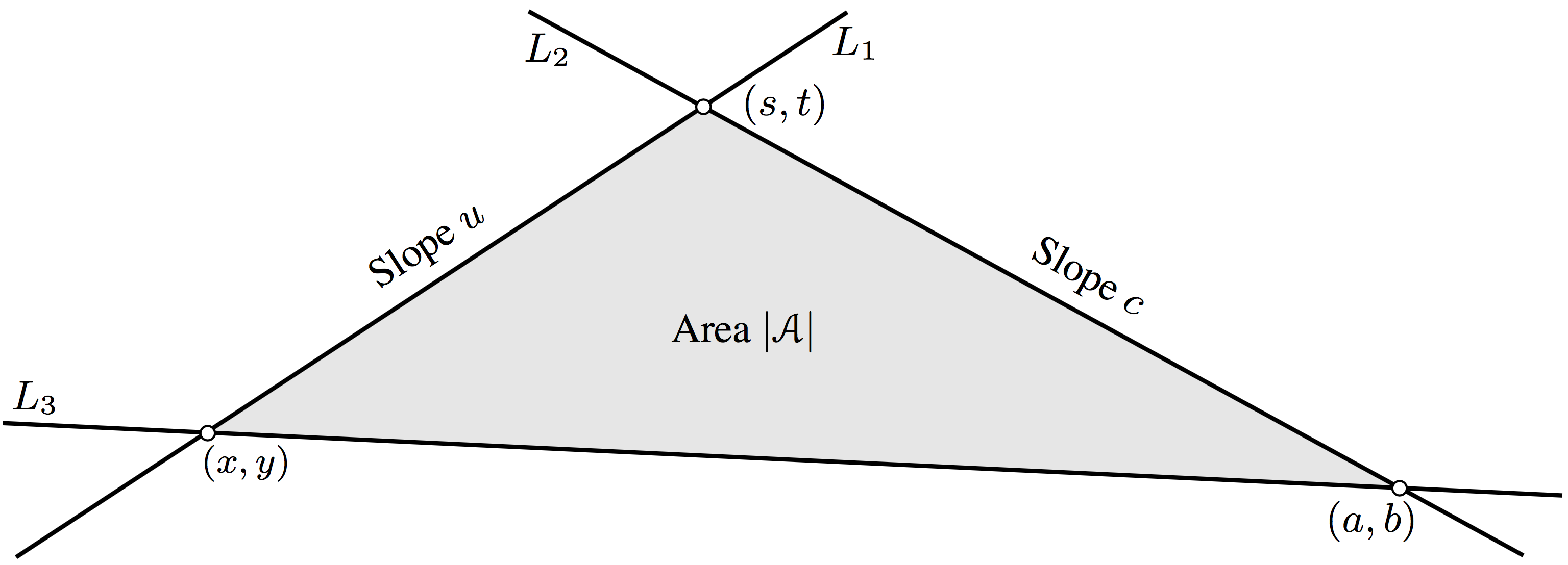
Figure 1. Geometric construction of the joint invariant $\mathcal{A}$.

For the second interpretation, let us first recall a classical construction. Fix $p_{0}\in\mathbb{R}^{2}$ and a line $L_{0}$ through $p_{0}$. Given any line $L$ through $p_{0}$ that is transverse to $L_{0}$, consider a hyperbola ${\mathcal{H}}$ having asymptotes $L_{0}$ and $L$. For any point $p\in{\mathcal{H}}$, we can form the:

• asymptotes-parallelogram with vertices $p$ and $p_{0}$ and sides parallel to $L$ and $L_{0}$.

• tangent-asymptotes-triangle whose vertices are $p_{0}$ and the intersection points of tangent line to ${\mathcal{H}}$ at $p$ with the asymptotes $L$ and $L_{0}$.

Two well-known facts from classical geometry about this construction are:

• One of the diagonals of the asymptotes parallelogram (the one not passing through $p$ and $p_{0}$) is itself parallel to the tangent line to ${\mathcal{H}}$ at $p$.

• The area of the asymptotes-parallelogram, which we denote by $\operatorname{Area}({\mathcal{H}})$, is half that of the tangent-asymptotes-triangle. Moreover, these areas are constant for any choice of $p\in{\mathcal{H}}$.

This gives a natural equi-affinely invariant construction: Fix ${\mathcal{A}}$ and fix $(a,b,c)\in J^{1}(\mathbb{R},\mathbb{R})$. The latter determines a point $p_{0}:=(a,b)\in\mathbb{R}^{2}$ and line $L_{0}$ with slope $c$, and we consider the family of all hyperbolas ${\mathcal{H}}$ having $L_{0}$ as one asymptote and having $\operatorname{Area}({\mathcal{H}})=|{\mathcal{A}}|$. This gives a local foliation of (an open subset of) the plane, as the example below illustrates. The collection of all such foliations is $\operatorname{SAff}(2,\mathbb{R})$-invariant.

Example 5.2.

Fix ${\mathcal{A}}$. When $(a,b,c)=(0,0,0)$, solving (5.4) for $u=y^{\prime}$ gives the ODE $y^{\prime}=\frac{y^{2}}{xy+2{\mathcal{A}}}$. Rewrite this as $0=\frac{dx}{y}-\frac{xy+2{\mathcal{A}}}{y^{3}}dy=\frac{dx}{y}-\frac{x}{y^{2}}dy+\frac{2{\mathcal{A}}}{y^{3}}$, with general solution $\frac{x}{y}+\frac{{\mathcal{A}}}{y^{2}}=\mu\in\mathbb{R}$. Rearranging gives $y(\mu y-x)={\mathcal{A}}$, which are hyperbolas ${\mathcal{H}}_{\mu}$ with asymptotes $y=0$ and $y=\frac{x}{\mu}$. A simple exercise shows that $\operatorname{Area}({\mathcal{H}}_{\mu})=|{\mathcal{A}}|$, independent of $\mu$.

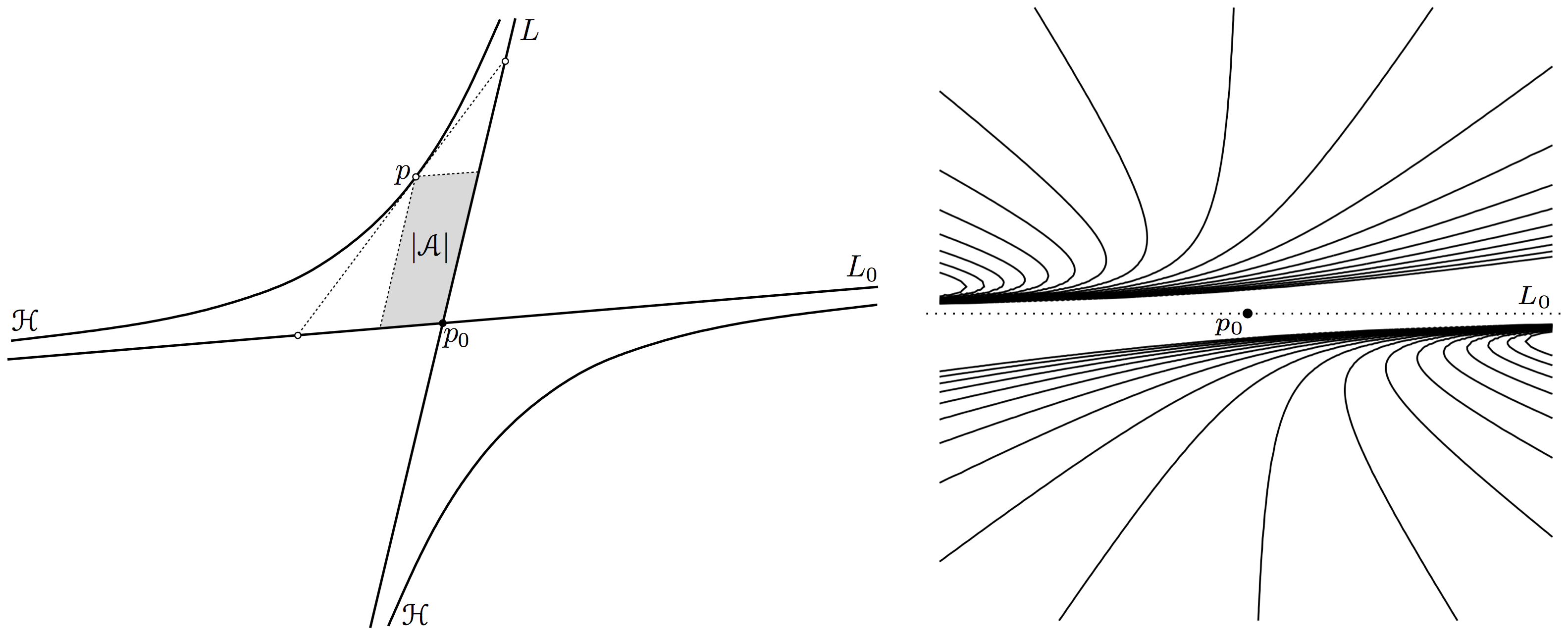
Figure 2. Asymptotes-parallelogram and a foliation by hyperbolas with constant area

5.5. Related PDE realization

Let us now describe the compatible, complete system of 2nd order PDEs (§1.2) that corresponds to the ASD-ILC structure (3.3) with symmetry ${\mathfrak{g}}=\mathfrak{saff}(2,{\mathbb{C}})$. In other words, we are looking for the equations whose complete solution $w(z_{1},z_{2})$ is defined by (5.5). By definition, this system of PDEs admits the 5-dimensional Lie algebra of point symmetries (5.6), which coincides with the lift of ${\mathfrak{g}}$ to $J^{1}({\mathbb{C}},{\mathbb{C}})$ as defined in §5.2. We identify here $J^{1}({\mathbb{C}},{\mathbb{C}})$ with ${\mathbb{C}}^{3}=J^{0}({\mathbb{C}}^{2},{\mathbb{C}})$ equipped with coordinates $(z_{1},z_{2},w)$ and then further prolong ${\mathfrak{g}}$ to $J^{2}({\mathbb{C}}^{2},{\mathbb{C}})$ to determine all ${\mathfrak{g}}$-invariant complete systems of 2nd order on $w(z_{1},z_{2})$.

All such systems were computed in the PhD thesis of Hillgarter [12]. The ${\mathfrak{g}}$-action lifted to $J^{2}({\mathbb{C}}^{2},{\mathbb{C}})$ admits the following three absolute invariants (see p.83 (${\textbf{ip}_{13}}$) and §4.2.1 of [12]):

$$I_{1} =\frac{w_{1}^{2}w_{22}+w_{2}^{2}w_{11}-2w_{1}w_{2}w_{12}}{(w_{1}+ww_{2})^{2}},$$

$$I_{2} =\frac{w_{1}w_{12}-w_{2}w_{11}+w(w_{1}w_{22}-w_{2}w_{12})}{(w_{1}+ww_{2})^{5/3}},$$

$$I_{3} =\frac{w_{11}+w^{2}w_{22}-2w_{1}w_{2}+2w(w_{12}-w_{2}^{2})}{(w_{1}+ww_{2})^{4/3}}.$$

So, any system of 2nd order PDEs admitting point symmetry ${\mathfrak{g}}$ is (implicitly) given by:

$$\{I_{1}=\alpha_{1},\quad I_{2}=\alpha_{2},\quad I_{3}=\alpha_{3}\},$$ (5.12)

where $\alpha_{i}\in\mathbb{C}$. We now classify those that are compatible, i.e. $E$ from (2.1) is Frobenius-integrable.

Proposition 5.3.

All compatible, complete 2nd order PDE systems $w_{ij}=f_{ij}(z_{k},w,w_{\ell})$, $1\leq i,j,k,\ell\leq 2$ that are invariant under (5.6) are equivalent to one of:

$$\begin{array}[]{|c|c|c|}\hline\cr\begin{cases}I_{1}=i,\\ I_{2}=3(4^{-1/3})e^{-i\pi/3},\\ I_{3}=-3(4^{1/3})e^{-i\pi/6}\end{cases}&\begin{cases}w_{11}=\frac{w_{1}^{2}}{(w_{2}w+w_{1})^{2/3}}+\frac{2w_{1}^{2}w_{2}}{w_{2}w+w_{1}},\\ w_{12}=\frac{w_{1}w_{2}}{(w_{2}w+w_{1})^{2/3}}+\frac{2w_{1}w_{2}^{2}}{w_{2}w+w_{1}},\\ w_{22}=\frac{w_{2}^{2}}{(w_{2}w+w_{1})^{2/3}}+\frac{2w_{2}^{3}}{w_{2}w+w_{1}}\end{cases}&\begin{cases}w_{11}=\frac{2w_{1}^{2}w_{2}}{w_{2}w+w_{1}},\\ w_{12}=\frac{2w_{1}w_{2}^{2}}{w_{2}w+w_{1}},\\ w_{22}=\frac{2w_{2}^{3}}{w_{2}w+w_{1}}\end{cases}\\ \hline\cr\mbox{Type }\mbox{$\mathsf{I}$}&\mbox{Type }\mbox{$\mathsf{II}$}&\mbox{Type }\mbox{$\mathsf{III}$}\\ \hline\cr\mbox{ASD}&\mbox{not ASD}&\mbox{not ASD}\\ \hline\cr\end{array}$$ (5.16)

For the type $\mathsf{I}$ and $\mathsf{II}$ systems above, (5.6) is the full point symmetry algebra, while the type $\mathsf{III}$ system admits the additional point symmetry $z_{1}\partial_{z_{1}}+z_{2}\partial_{z_{2}}$ and full point symmetry algebra $\mathfrak{aff}(2,\mathbb{C})$.

Proof.

Solving (5.12) for $w_{ij}$, we find that (5.12) is compatible if and only if $3\alpha_{1}\alpha_{3}=4\alpha_{2}^{2}$ and $9\alpha_{1}=\alpha_{2}\alpha_{3}$. This admits the following solutions:

1. $(\alpha_{1},\alpha_{2},\alpha_{3})=(0,0,\alpha)$: If $\alpha=0$, we get the third system. If $\alpha\neq 0$, we normalize it to $\alpha=1$ using the rescaling $(z_{1},z_{2},w)\mapsto(\lambda z_{1},\lambda z_{2},w)$, which induces $(I_{1},I_{2},I_{3})\mapsto(\lambda^{-2}I_{1},\lambda^{-4/3}I_{2},\lambda^{-2/3}I_{3})$. This gives the second system.

2. $(\alpha_{1},\alpha_{2},\alpha_{3})=(\frac{\alpha^{3}}{108},\frac{\alpha^{2}}{12},\alpha)$: Evaluating $I_{1},I_{2},I_{3}$ on the functions $w(z_{1},z_{2})$ defined by (5.4), we find that $\alpha=-3(\frac{4}{{\mathcal{A}}})^{1/3}$. (As expected, this does not depend on the parameters $(a_{1},a_{2},c)$, but only on ${\mathcal{A}}$.) Rescaling as above, we normalize ${\mathcal{A}}=i$, which gives the first system.

Applying (2.16), we identify the root types of ${\mathcal{Q}}_{4}$ as indicated. For the type $\mathsf{I}$ and $\mathsf{II}$ cases, (2.20) confirms 5-dimensional symmetry, while there is the additional indicated symmetry for type $\mathsf{III}$ case. (From [7, Table 2], this is a realization of model $\mathsf{III}$.6-2.) From Proposition 3.3 and Example 2.10, an $\mathfrak{saff}(2,\mathbb{C})$-invariant ASD-ILC structure must be of type $\mathsf{I}$. ∎

The type $\mathsf{I}$ realization above is the desired PDE system with associated CR hypersurface (5.5).

6. Simply-transitive tubular hypersurfaces

6.1. From homogeneous tubes to algebraic data

Given a real affine hypersurface ${\mathcal{S}}\subset\mathbb{R}^{n+1}$, we discussed in §1 its associated tubular CR hypersurface $M_{\mathcal{S}}\subset\mathbb{C}^{n+1}$, and its complexification $M^{c}_{\mathcal{S}}\subset\mathbb{C}^{n+1}\times\mathbb{C}^{n+1}$ is the associated tubular ILC hypersurface. (We recover $M_{\mathcal{S}}$ as the fixed-point set of the anti-involution $\tau(z,a)=(\overline{a},\overline{z})$ restricted to $M^{c}_{\mathcal{S}}$.) The symmetry algebra $\operatorname{sym}(M^{c}_{\mathcal{S}})$ is the complex Lie algebra consists of all holomorphic vector fields $X=\xi^{k}(z)\partial_{z_{k}}+\sigma^{k}(a)\partial_{a_{k}}\in{\mathfrak{X}}(\mathbb{C}^{n+1})\times{\mathfrak{X}}(\mathbb{C}^{n+1})$ that are everywhere tangent to $M^{c}_{\mathcal{S}}$. The affine symmetry algebra $\mathfrak{aff}({\mathcal{S}})$ consists of those affine vector fields ${\mathbf{S}}=(A_{k\ell}x_{\ell}+b_{k})\partial_{x_{k}}$, for $A_{k\ell},b_{k}\in\mathbb{R}$, that are everywhere tangent to ${\mathcal{S}}$. Any ${\mathbf{S}}\in\mathfrak{aff}({\mathcal{S}})$ induces symmetries of ${\mathbf{S}}^{\operatorname{cr}}$ of $M_{\mathcal{S}}$ and ${\mathbf{S}}^{\operatorname{lc}}$ of $M^{c}_{\mathcal{S}}$ as indicated below. We respectively denote the induced real and complex Lie algebras by $\mathfrak{aff}({\mathcal{S}})^{\operatorname{cr}}\subset\mathfrak{hol}(M_{\mathcal{S}})$ and $\mathfrak{aff}({\mathcal{S}})^{\operatorname{lc}}\subset\operatorname{sym}(M^{c}_{\mathcal{S}})$, and it is clear that $\mathfrak{aff}({\mathcal{S}})^{\operatorname{lc}}\cong\mathfrak{aff}({\mathcal{S}})^{\operatorname{cr}}\otimes_{\mathbb{R}}\mathbb{C}\cong\mathfrak{aff}({\mathcal{S}})\otimes_{\mathbb{R}}\mathbb{C}$.

Real affine hypersurface ${\mathcal{S}}=\{x:{\mathcal{F}}(x)=0\}\subset\mathbb{R}^{n+1}$,  $d{\mathcal{F}}\neq 0$ on ${\mathcal{S}}$; Real affine symmetry ${\mathbf{S}}=(A_{k\ell}x_{\ell}+b_{k})\partial_{x_{k}}\in\mathfrak{aff}({\mathcal{S}})$

Tubular CR hypersurface $M_{\mathcal{S}}=\{z:{\mathcal{F}}(\operatorname{Re}z)=0\}\subset\mathbb{C}^{n+1}$; $i\partial_{z_{1}},...,i\partial_{z_{n+1}}\in\mathfrak{hol}(M_{\mathcal{S}})$, ${\mathbf{S}}^{\operatorname{cr}}:=(A_{k\ell}z_{\ell}+b_{k})\partial_{z_{k}}\in\mathfrak{aff}({\mathcal{S}})^{\operatorname{cr}}$ Tubular ILC hypersurface $M^{c}_{\mathcal{S}}=\{(z,a):{\mathcal{F}}(\frac{z+a}{2})=0\}\subset\mathbb{C}^{n+1}\times\mathbb{C}^{n+1}$; $\partial_{z_{1}}-\partial_{a_{1}},...,\partial_{z_{n+1}}-\partial_{a_{n+1}}\in\operatorname{sym}(M^{c}_{\mathcal{S}})$, ${\mathbf{S}}^{\operatorname{lc}}:=(A_{k\ell}z_{\ell}+b_{k})\partial_{z_{k}}+(A_{k\ell}a_{\ell}+b_{k})\partial_{a_{k}}\in\mathfrak{aff}({\mathcal{S}})^{\operatorname{lc}}$

Remark 6.1.

Any complex affine hypersurface ${\mathcal{S}}\subset\mathbb{C}^{n+1}$ also induces a tubular ILC hypersurface $M^{c}_{\mathcal{S}}\subset\mathbb{C}^{n+1}\times\mathbb{C}^{n+1}$ via the same prescription above.

For $M^{c}_{\mathcal{S}}$, note that ${\mathfrak{a}}=\langle\partial_{z_{1}}-\partial_{a_{1}},\ldots,\partial_{z_{n+1}}-\partial_{a_{n+1}}\rangle$ is an $(n+1)$-dimensional abelian Lie algebra ${\mathfrak{a}}\subset{\mathfrak{g}}:=\operatorname{sym}(M^{c}_{\mathcal{S}})$ that is transverse to $E$ and $F$ (as defined in §1.2), so we are naturally led to the following algebraic data for any holomorphically homogeneous tube:

Definition 6.2.

A tubular CR realization for an ILC quadruple $({\mathfrak{g}},{\mathfrak{k}};{\mathfrak{e}},{\mathfrak{f}})$ in dimension ${\rm dim}({\mathfrak{g}}/{\mathfrak{k}})=2n+1$ is a pair $({\mathfrak{a}},\tau)$, where

1. ${\mathfrak{a}}\subset{\mathfrak{g}}$ is an $(n+1)$-dimensional abelian subalgebra;

2. ${\mathfrak{e}}\cap{\mathfrak{a}}={\mathfrak{f}}\cap{\mathfrak{a}}=0$.

3. $\tau$ is an admissible anti-involution of $({\mathfrak{g}},{\mathfrak{k}};{\mathfrak{e}},{\mathfrak{f}})$ that preserves ${\mathfrak{a}}$.

Conversely, given such data as above, we integrate $({\mathfrak{g}},{\mathfrak{k}})$ to a (local) homogeneous space $N=G/K$ with $G$-invariant distributions $E,F$. Since $C=E\oplus F$ is non-degenerate, then all symmetries of the ILC structure $(N;E,F)$ are in 1-1 correspondence with their projection by $d\pi_{1}$ or $d\pi_{2}$. (We refer to the double fibration (1.10).) This implies that the direct product of $\pi_{1}$ and $\pi_{2}$ gives a local embedding $N\to N/E\times N/F$ (with codomain being locally $\mathbb{C}^{n+1}\times\mathbb{C}^{n+1}$). As ${\mathfrak{a}}$ is abelian, we can identify it with $\mathbb{C}^{n+1}$, with the anti-involution $\tau$ acting on it as $w\mapsto-\bar{w}$ (in the standard basis ${\mathbf{b}}$ on $\mathbb{C}^{n+1}$). Let $A\subset G$ be the corresponding subgroup, which can also be locally identified with ${\mathbb{C}}^{n+1}$ equipped with the same anti-involution. Due to (T.1) and (T.2) the action of $A$ on both $N/E$ and $N/F$ is (locally) simply transitive. So, we can identify both $N/E$ and $N/F$ with some open subsets of $\mathbb{C}^{n+1}$, on which we introduce local coordinates $z$ and $a$ relative to ${\mathbf{b}}$ and $-{\mathbf{b}}$ respectively. Hence, ${\mathfrak{a}}=\langle\partial_{z_{k}}-\partial_{a_{k}}\rangle$.

Since $\tau$ swaps ${\mathfrak{f}}$ and ${\mathfrak{e}}$, it extends to the direct product $N/E\times N/F$ as $\widetilde{\tau}(z,a)=(\bar{a},\bar{z})$. The embedding $N\hookrightarrow N/E\times N/F\cong_{{\rm loc}}\mathbb{C}^{n+1}\times\mathbb{C}^{n+1}$ is given by a single complex analytic equation $\Phi(z,a)=0$. Invariance of $N$ under ${\mathfrak{a}}$ forces $N=\{(z,a):{\mathcal{F}}((z+a)/2)=0\}$. Finally, taking the slice of ${\mathbb{C}}^{n+1}\times{\mathbb{C}}^{n+1}$ defined as a fixed-point set of $\widetilde{\tau}$, we arrive at the tubular hypersurface $M_{{\mathcal{S}}}=\{z\colon{\mathcal{F}}(\operatorname{Re}z)=0\}\subset{\mathbb{C}}^{n+1}$, where ${\mathcal{F}}$ is now real-valued. It is a tube over the base ${\mathcal{S}}=\{x:{\mathcal{F}}(x)=0\}\subset\mathbb{R}^{n+1}$.

Lemma 6.3.

${\mathfrak{n}}({\mathfrak{a}})/{\mathfrak{a}}\cong\mathfrak{aff}({\mathcal{S}})\otimes_{\mathbb{R}}\mathbb{C}$.

Proof.

Clearly, $\mathrm{span}_{\mathbb{C}}\{{\mathbf{S}}^{\operatorname{lc}}:{\mathbf{S}}\in\mathfrak{aff}({\mathcal{S}})\}\oplus{\mathfrak{a}}\subset{\mathfrak{n}}({\mathfrak{a}})$. Conversely, if $X=\xi^{k}(z)\partial_{z_{k}}+\sigma^{k}(a)\partial_{a_{k}}$ normalizes ${\mathfrak{a}}=\langle\partial_{z_{1}}-\partial_{a_{1}},\ldots,\partial_{z_{n+1}}-\partial_{a_{n+1}}\rangle$, then $X=(A_{k\ell}z_{\ell}+b_{k})\partial_{z_{k}}+(A_{k\ell}a_{\ell}+c_{k})\partial_{a_{k}}$ for some $A_{k\ell},b_{k},c_{k}\in{\mathbb{C}}$. Adding $(\frac{c_{k}-b_{k}}{2})(\partial_{z_{k}}-\partial_{a_{k}})\in{\mathfrak{a}}$, we may assume that $b_{k}=c_{k}$. Since ${\mathfrak{a}}$ is stable under $d\tau$ (where $\tau(z,a)=(\bar{a},\bar{z})$), then so is ${\mathfrak{n}}({\mathfrak{a}})$. Since $\tau^{2}=\mathrm{id}$, we can decompose ${\mathfrak{n}}({\mathfrak{a}})$ into $\pm 1$ eigenspaces for $d\tau$. Modulo ${\mathfrak{a}}$, the $+1$ eigenspace consists of $X=(A_{k\ell}z_{\ell}+b_{k})\partial_{z_{k}}+(A_{k\ell}a_{\ell}+b_{k})\partial_{a_{k}}\in{\mathfrak{n}}({\mathfrak{a}})$ with $A_{k\ell},b_{k}\in\mathbb{R}$, hence $X={\mathbf{S}}^{\operatorname{lc}}$, where ${\mathbf{S}}=(A_{k\ell}x_{\ell}+b_{k})\partial_{x_{k}}\in\mathfrak{aff}({\mathcal{S}})$. The $-1$ eigenspace consists of similar vector fields, but with $A_{k\ell},b_{k}\in i\mathbb{R}$. Thus, ${\mathfrak{n}}({\mathfrak{a}})\equiv\mathrm{span}_{\mathbb{C}}\{{\mathbf{S}}^{\operatorname{lc}}:{\mathbf{S}}\in\mathfrak{aff}({\mathcal{S}})\}\,{\rm mod}\ {\mathfrak{a}}$, which implies the claim. ∎

Corollary 6.4.

Let $M^{5}\subset\mathbb{C}^{3}$ be a holomorphically simply-transitive, Levi non-degenerate hypersurface with $\mathfrak{hol}(M)$ containing a 3-dimensional abelian ideal. Then $M$ is a tube on an affinely simply-transitive base.

Proof.

By (1.12), the induced ILC structure on $M^{c}$ is simply-transitive, so can be encoded by an ASD-ILC triple $({\mathfrak{g}};{\mathfrak{e}},{\mathfrak{f}})$, where ${\mathfrak{g}}=\operatorname{sym}(M^{c})=\mathfrak{hol}(M)\otimes_{\mathbb{R}}\mathbb{C}$ is 5-dimensional and admits some admissible anti-involution $\tau$. By hypothesis, $\mathfrak{hol}(M)$ contains a 3-dimensional abelian ideal, so there exists a 3-dimensional abelian ideal ${\mathfrak{a}}\subset{\mathfrak{g}}$.

Applying Theorem 4.1, we get ${\mathfrak{a}}=\tau({\mathfrak{a}})$ and ${\mathfrak{e}}\cap{\mathfrak{a}}={\mathfrak{f}}\cap{\mathfrak{a}}=0$. Thus, $({\mathfrak{a}},\tau)$ is a tubular CR realization for the ILC triple $({\mathfrak{g}};{\mathfrak{e}},{\mathfrak{f}})$. Since ${\mathfrak{a}}$ is an ideal in ${\mathfrak{g}}$, then ${\mathfrak{g}}/{\mathfrak{a}}={\mathfrak{n}}({\mathfrak{a}})/{\mathfrak{a}}\cong\mathfrak{aff}({\mathcal{S}})\otimes_{\mathbb{R}}\mathbb{C}$ for some base ${\mathcal{S}}$ as constructed above. As $\mathfrak{hol}(M)$ is transitive on $M$, we see that the projection $\mathfrak{hol}(M)$ onto ${\mathcal{S}}$ is also transitive. Thus, ${\mathcal{S}}$ is affinely simply-transitive. ∎

Given $p\in\mathbb{C}^{n+1}$, there is a natural isomorphism of the Lie algebra of all (real or complex) affine vector fields with $\mathfrak{aff}(n+1,\mathbb{C}):=\mathfrak{gl}(n+1,\mathbb{C})\ltimes\mathbb{C}^{n+1}$, via

$$(A_{k\ell}(z_{\ell}-p_{\ell})+b_{k})\partial_{z_{k}}\quad\mapsto\quad(A,b),$$ (6.1)

for which $A$ is the linear part at $p$, and $b$ is the translational part. Recall that conjugation by $P\in\mathsf{GL}(n+1,\mathbb{C})\subset\operatorname{Aff}(n+1,\mathbb{C})$ induces the action $(A,b)\mapsto(PAP^{-1},Pb)$. Finally, $\mathfrak{aff}(n+1,\mathbb{C})$ has a unique abelian ideal consisting of translations $\langle\partial_{x_{k}}\rangle\cong\mathbb{C}^{n+1}$.

Proposition 6.5.

Let ${\mathcal{S}}\subset\mathbb{R}^{n+1}$ be an affinely homogeneous hypersurface with non-degenerate 2nd fundamental form. Then the tubular ILC hypersurface $M_{\mathcal{S}}^{c}\subset\mathbb{C}^{n+1}\times\mathbb{C}^{n+1}$ is homogeneous and encoded by an ILC quadruple $({\mathfrak{g}},{\mathfrak{k}};{\mathfrak{e}},{\mathfrak{f}})$, given for any $p\in{\mathcal{S}}$ by

$${\mathfrak{e}}:=\mathfrak{aff}({\mathcal{S}})\otimes_{\mathbb{R}}\mathbb{C},\quad{\mathfrak{g}}:={\mathfrak{e}}\ltimes\mathbb{C}^{n+1},\quad{\mathfrak{f}}:=\{Y\in{\mathfrak{g}}:Y|_{p}=0\},\quad{\mathfrak{k}}:={\mathfrak{e}}\cap{\mathfrak{f}}.$$ (6.2)

Proof.

Since ${\mathcal{S}}$ is affinely homogeneous, then $M^{c}_{\mathcal{S}}$ is homogeneous, with $\operatorname{sym}(M^{c}_{\mathcal{S}})$ containing

$${\mathfrak{g}}=\mathfrak{aff}({\mathcal{S}})^{\operatorname{lc}}\oplus\mathrm{span}_{\mathbb{C}}\{\partial_{z_{1}}-\partial_{a_{1}},\ldots,\partial_{z_{n+1}}-\partial_{a_{n+1}}\},$$ (6.3)

which is transitive on $M^{c}_{\mathcal{S}}$. Given $p\in{\mathcal{S}}$, we have $(p,p)\in M^{c}_{\mathcal{S}}$ and

$${\mathfrak{e}}=\{Y\in{\mathfrak{g}}:d\pi_{2}|_{(p,p)}(Y)=0\},\quad{\mathfrak{f}}=\{Y\in{\mathfrak{g}}:d\pi_{1}|_{(p,p)}(Y)=0\},\quad{\mathfrak{k}}={\mathfrak{e}}\cap{\mathfrak{f}},$$ (6.4)

in terms of the double fibration (1.10). Explicitly, let $X:=(A_{k\ell}x_{\ell}+b_{k})\partial_{x_{k}}\in\mathfrak{aff}({\mathcal{S}})$ and $T_{X,p}:=(A_{k\ell}p_{\ell}+b_{k})(\partial_{z_{k}}-\partial_{a_{k}})\in\operatorname{sym}(M_{\mathcal{S}}^{c})$, where $p=(p_{1},\ldots,p_{n+1})\in{\mathcal{S}}$. Consider

$$X^{\operatorname{lc}}+T_{X,p} =(A_{k\ell}(z_{\ell}+p_{\ell})+2b_{k})\partial_{z_{k}}+A_{k\ell}(a_{\ell}-p_{\ell})\partial_{a_{k}},$$ (6.5)

$$X^{\operatorname{lc}}-T_{X,p} =A_{k\ell}(z_{\ell}-p_{\ell})\partial_{z_{k}}+(A_{k\ell}(a_{\ell}+p_{\ell})+2b_{k})\partial_{a_{k}}.$$ (6.6)

Clearly, ${\mathfrak{e}}=\mathrm{span}_{\mathbb{C}}\{X^{\operatorname{lc}}+T_{X,p}:X\in\mathfrak{aff}({\mathcal{S}})\}$, while ${\mathfrak{f}}=\mathrm{span}_{\mathbb{C}}\{X^{\operatorname{lc}}-T_{X,p}:X\in\mathfrak{aff}({\mathcal{S}})\}$.

Since $C=E\oplus F$ is non-degenerate, then all elements of $\operatorname{sym}(M^{c})$ are in 1-1 correspondence with their projection by either $d\pi_{1}$ or $d\pi_{2}$. Focusing on their $d\pi_{1}$ projections, it is clear that $(d\pi_{1}({\mathfrak{g}}),d\pi_{1}({\mathfrak{f}}))$ agree with $({\mathfrak{g}},{\mathfrak{f}})$ in (6.2). Letting $\mathcal{D}\in\operatorname{Aff}(n+1,\mathbb{C})$ be the dilation centered at $p$ by a factor $\frac{1}{2}$, define $(\bar{\mathfrak{g}},\bar{\mathfrak{k}};\bar{\mathfrak{e}},\bar{\mathfrak{f}})$ be the (isomorphic) projection of $({\mathfrak{g}},{\mathfrak{k}};{\mathfrak{e}},{\mathfrak{f}})$ by $d{\mathcal{D}}\circ d\pi_{1}$. Let us view this in terms of (6.1). Letting $v=Ap+b$ and $D=\frac{1}{2}\,\mathrm{id}$, (6.5) and (6.6) become:

$$(A,2v)\mapsto(DAD^{-1},2Dv)=(A,v),\qquad(A,0)\mapsto(DAD^{-1},0)=(A,0).$$ (6.7)

Via (6.1), the former is $(A_{k\ell}z_{\ell}+b_{k})\partial_{z_{k}}$. Thus, after dropping bars, $(\bar{\mathfrak{g}},\bar{\mathfrak{k}};\bar{\mathfrak{e}},\bar{\mathfrak{f}})$ agrees with (6.2). ∎

Note that ${\mathfrak{f}}\subset{\mathfrak{g}}$ is the isotropy subalgebra at $p$. Using (2.21) and Proposition 6.5, the quartic ${\mathcal{Q}}_{4}$ can be efficiently computed for tubes $M^{c}_{\mathcal{S}}$ over affinely simply-transitive ${\mathcal{S}}$ (see Table 3).

6.2. Tubes on affinely simply-transitive surfaces

We finally address the tubular simply-transitive Levi non-degenerate classification. From our work above, these can all be described as tubes on an affinely simply-transitive base. For the latter, we will use the DKR classification [6] of surfaces in real affine 3-space and proceed with the initial steps described in §1.1.

From the DKR list, we begin by excluding those surfaces whose associated tube already explicitly appears in the multiply-transitive classification [8]. In Table 2, these known tubes are indicated with their ILC quartic types and symmetry dimensions, keeping in mind (1.12). (The additional hyphenated suffix, e.g. $\mathsf{D}$.6-1 and $\mathsf{D}$.6-2, indicates labelling of different families derived from [7].) Finally, we restrict to affinely simply-transitive surfaces with non-degenerate Hessians. This excludes quadrics, cylinders, and the Cayley surface $u=x_{1}x_{2}-\frac{x_{1}^{3}}{3}$. (The last of these admits the affine symmetries $x_{1}\partial_{x_{1}}+2x_{2}\partial_{x_{2}}+3u\partial_{u}$, $\partial_{x_{1}}+x_{1}\partial_{x_{2}}+x_{2}\partial_{u}$, and $\partial_{x_{2}}+x_{1}\partial_{u}$.)

$$\begin{array}[]{|c|c|l|l|cccc}\hline\cr\mbox{DKR label}&\mbox{Non-degenerate real affine surface}&\mbox{ILC Classification \cite[cite]{[\@@bibref{}{ILC}{}{}]}}\\ \hline\cr\hline\cr(3)&\begin{array}[]{c}u=\ln(x_{1})+\alpha\ln(x_{2})\\ {\scriptstyle(\alpha\neq 0)}\end{array}&\begin{tabular}[]{@{}l@{}}\mbox{$\mathsf{D}$.7}: $\alpha\neq 0,-1$;\\ \mbox{$\mathsf{O}$.15}: $\alpha=-1$\end{tabular}\\ \hline\cr(4)&u=\alpha\arg(ix_{1}+x_{2})+\ln(x_{1}^{2}+x_{2}^{2})&\mbox{$\mathsf{D}$.7}\\ &u=\arg(ix_{1}+x_{2})&\mbox{$\mathsf{O}$.15}\\ \hline\cr(7)&u=x_{2}^{2}+\epsilon e^{x_{1}}&\mbox{$\mathsf{O}$.15}\\ \hline\cr(8)&\begin{array}[]{c}u=x_{2}^{2}+\epsilon x_{1}^{\alpha}\\ {\scriptstyle(\alpha\neq 0,1)}\end{array}&\begin{tabular}[]{@{}l@{}}\mbox{$\mathsf{D}$.6-2}: $\alpha\neq 0,1,2$;\\ \mbox{$\mathsf{O}$.15}: $\alpha=2$\\ \end{tabular}\\ \hline\cr(9)&u=x_{2}^{2}+\epsilon\ln(x_{1})&\mbox{$\mathsf{D}$.7}\\ \hline\cr(10)&u=x_{2}^{2}+\epsilon x_{1}\ln(x_{1})&\mbox{$\mathsf{D}$.6-2}\\ \hline\cr(11)&u=x_{1}x_{2}+e^{x_{1}}&\mbox{$\mathsf{N}$.6-2}\\ \hline\cr(12)&u=x_{1}x_{2}+x_{1}^{\alpha}&\begin{tabular}[]{@{}l@{}}\mbox{$\mathsf{N}$.6-1}: $\alpha\neq 0,1,2,3,4$;\\ \mbox{$\mathsf{N}$.8}: $\alpha=4$;\\ \mbox{$\mathsf{O}$.15}: $\alpha=0,1,2,3$\end{tabular}\\ \hline\cr(13)&u=x_{1}x_{2}+\ln(x_{1})&\mbox{$\mathsf{N}$.6-1}\\ \hline\cr(14)&u=x_{1}x_{2}+x_{1}\ln(x_{1})&\mbox{$\mathsf{N}$.7-2}\\ \hline\cr(15)&u=x_{1}x_{2}+x_{1}^{2}\ln(x_{1})&\mbox{$\mathsf{N}$.6-1}\\ \hline\cr(17)&x_{1}u=x_{2}^{2}+\epsilon x_{1}\ln(x_{1})&\mbox{$\mathsf{D}$.6-1}\\ \hline\cr\end{array}$$

Table 2. Affinely simply-transitive surfaces with holomorphically multiply-transitive associated tubes. Parameters $\alpha\in\mathbb{R}$ and $\epsilon=\pm 1$.

Remark 6.6.

Family (4) was originally stated in [6] as $u=\alpha\arg(ix_{1}+x_{2})+\beta\ln(x_{1}^{2}+x_{2}^{2})$. Scaling $u$ yields the two cases in Table 2, the first of which explicitly appears in [8]. The tube $M$ over $u=\arg(ix_{1}+x_{2})$ is mapped to the hyperquadric $\operatorname{Im}\widetilde{w}=|\widetilde{z}_{1}|^{2}-|\widetilde{z}_{2}|^{2}$ by

$$(\widetilde{z}_{1},\widetilde{z}_{2},\widetilde{w})=\left(\frac{1}{\sqrt{2}}\Big{(}e^{iw}-\frac{z_{1}-iz_{2}}{4}\Big{)},\frac{1}{\sqrt{2}}\Big{(}e^{iw}+\frac{z_{1}-iz_{2}}{4}\Big{)},e^{iw}\Big{(}\frac{iz_{1}-z_{2}}{2}\Big{)}\right).$$ (6.8)

Thus, ${\rm dim}\,\mathfrak{hol}(M)=15$ and $M$ is flat. The above was derived from [13, Thm.6.1(6) & (6.69)].

Model (16) when $\alpha=0$ gives the quadric $x_{1}u=x_{2}^{2}+\epsilon$, with affine symmetries: $x_{1}\partial_{x_{1}}-u\partial_{u}$, $2x_{2}\partial_{x_{1}}+u\partial_{x_{2}}$, and $x_{1}\partial_{x_{2}}+2x_{2}\partial_{u}$. Its associated tube admits $\mathfrak{so}(1,2)\ltimes{\mathbb{R}}^{3}$ symmetry.

All remaining surfaces are given in Table 1, and their affine symmetries ${\mathbf{S}},{\mathbf{T}}$ are given in Table 3. The associated tubes $M$ admit symmetries ${\mathbf{S}}^{\operatorname{cr}},{\mathbf{T}}^{\operatorname{cr}},i\partial_{z_{1}},i\partial_{z_{2}},i\partial_{w}\in\mathfrak{hol}(M)$, so ${\rm dim}\,\mathfrak{hol}(M)\geq 5$. In Table 3, we compute ${\mathcal{Q}}_{4}$ using (2.21) and Proposition 6.5, and classify its root type. (For details, we refer to a Maple file in our arXiv submission.) By (2.20), those of type $\mathsf{I}$ and $\mathsf{II}$ are confirmed to have ${\rm dim}\,\mathfrak{hol}(M)=5$, so only the type $\mathsf{D}$ and $\mathsf{N}$ cases remain. We used two methods to computationally confirm that ${\rm dim}\,\mathfrak{hol}(M)=5$ for these remaining cases: (i) PDE point symmetries (§6.3), and (ii) power series (§6.4).

$$\begin{array}[]{|c|@{}c@{}|@{}l@{}|@{}c@{}|l|c|}\hline\cr&\begin{tabular}[]{c}Generic point\\ $(x_{1},x_{2},u)$\\ on surface\end{tabular}&\begin{tabular}[]{l}Affine symmetries ${\mathbf{S}},{\mathbf{T}}$, isotropy fields $\widetilde{\mathbf{S}},\widetilde{\mathbf{T}}$,\\ and LC-adapted framing $\{{\mathbf{e}}_{1},{\mathbf{e}}_{2},{\mathbb{f}}_{1},{\mathbb{f}}_{2}\}$\end{tabular}&\mbox{ILC Quartic }{\mathcal{Q}}_{4}&\mbox{Root type of ${\mathcal{Q}}_{4}$}\\ \hline\cr\hline\cr\mathsf{T}1&(1,1,1)&\begin{array}[]{l}\begin{array}[]{@{}l@{}}{\mathbf{S}}=x_{1}\partial_{x_{1}}+\alpha u\partial_{u},\\ {\mathbf{T}}=x_{2}\partial_{x_{2}}+\beta u\partial_{u}\end{array}\quad\begin{array}[]{@{}l@{}}\widetilde{\mathbf{S}}={\mathbf{S}}-\partial_{x_{1}}-\alpha\partial_{u},\\ \widetilde{\mathbf{T}}={\mathbf{T}}-\partial_{x_{2}}-\beta\partial_{u}\end{array}\\ \hline\cr\begin{array}[]{@{}l}{\mathbf{e}}_{1}=\alpha{\mathbf{T}},\quad{\mathbf{e}}_{2}=\alpha\beta{\mathbf{S}}-\alpha(\alpha-1){\mathbf{T}},\\ {\mathbb{f}}_{1}=\frac{\alpha+\beta-1}{\alpha}\widetilde{\mathbf{S}},\quad{\mathbb{f}}_{2}=\widetilde{\mathbf{T}}-\frac{\beta-1}{\alpha}\widetilde{\mathbf{S}}\end{array}\end{array}&\begin{array}[]{l}(\alpha-1)(\alpha+2\beta-1)(\alpha+\beta-1)t^{4}\\ \quad+4(\alpha-1)(\beta-1)(\alpha+\beta-1)t^{3}\\ \quad+2(\alpha-1)(\beta-1)(\alpha+\beta-3)t^{2}\\ \quad-4(\alpha-1)(\beta-1)t\\ \quad+\frac{(\beta-1)(\beta+2\alpha-1)}{\alpha+\beta-1}\end{array}&\begin{tabular}[]{@{}l}Let $S(\alpha,\beta):=(\alpha-1)(\beta-1)(\alpha+\beta)$. Then:\\ \\ \mbox{$\mathsf{I}$}: $S(\alpha,\beta)\left(S(\alpha,\beta)+8\alpha\beta\right)\neq 0$\\ \mbox{$\mathsf{II}$}: $S(\alpha,\beta)=-8\alpha\beta$, excl. $\mbox{$\mathsf{D}$}$\\ \mbox{$\mathsf{D}$}: $(\alpha,\beta)=(-1,-1)$\\ \mbox{$\mathsf{N}$}: Exactly one of $\alpha=1$ or $\beta=1$ or $\beta=-\alpha$\\ \mbox{$\mathsf{O}$}: $(\alpha,\beta)\in\{(1,1),(1,-1),(-1,1)\}$\end{tabular}\\ \hline\cr\mathsf{T}2&(1,0,1)&\begin{array}[]{l}\begin{array}[]{@{}l@{}}{\mathbf{S}}=x_{1}\partial_{x_{1}}+x_{2}\partial_{x_{2}}+2\alpha u\partial_{u},\\ {\mathbf{T}}=x_{2}\partial_{x_{1}}-x_{1}\partial_{x_{2}}-\beta u\partial_{u}\end{array}\quad\begin{array}[]{l}\widetilde{\mathbf{S}}={\mathbf{S}}-\partial_{x_{1}}-2\alpha\partial_{u},\\ \widetilde{\mathbf{T}}={\mathbf{T}}+\partial_{x_{2}}+\beta\partial_{u}\end{array}\\ \hline\cr\alpha\neq 0:\\ \begin{array}[]{l}{\mathbf{e}}_{1}=\frac{1}{2\alpha-1}{\mathbf{S}},\quad{\mathbf{e}}_{2}=2\alpha{\mathbf{T}}+\beta{\mathbf{S}},\\ {\mathbb{f}}_{1}=(4\alpha^{2}+\beta^{2})\widetilde{\mathbf{S}},\quad{\mathbb{f}}_{2}=2\alpha\widetilde{\mathbf{T}}+\beta\widetilde{\mathbf{S}}\end{array}\\ \alpha=0:\\ \begin{array}[]{l}{\mathbf{e}}_{1}={\mathbf{T}},\quad{\mathbf{e}}_{2}={\mathbf{S}},\quad{\mathbb{f}}_{1}=\widetilde{\mathbf{S}},\quad{\mathbb{f}}_{2}=\widetilde{\mathbf{T}}-\beta\widetilde{\mathbf{S}}\end{array}\end{array}&\begin{array}[]{@{}l@{}}\begin{array}[]{l}-2(\alpha-1)(4\alpha^{2}+\beta^{2})^{2}t^{4}-8\beta(4\alpha^{2}+\beta^{2})t^{3}\\ \quad+\frac{4\left(4\alpha^{2}(2\alpha+1)(\alpha-1)+\beta^{2}(2\alpha^{2}+3\alpha-3)\right)}{2\alpha-1}t^{2}\\ \quad+\frac{8\beta}{2\alpha-1}t-\frac{2(\alpha-1)}{(2\alpha-1)^{2}},\quad\mbox{for}\quad\alpha\neq 0\end{array}\\ \\ \begin{array}[]{l}\beta(\beta^{2}+4),\quad\mbox{for}\quad\alpha=0\end{array}\end{array}&\begin{tabular}[]{@{}l}\mbox{$\mathsf{I}$}: $4\alpha(\alpha+1)^{2}+(\alpha+4)\beta^{2}\neq 0$, \mbox{ excl. \mbox{$\mathsf{N}$} \& \mbox{$\mathsf{O}$}}\\ \mbox{$\mathsf{II}$}: $4\alpha(\alpha+1)^{2}+(\alpha+4)\beta^{2}=0$, \mbox{ excl. \mbox{$\mathsf{D}$}}\\ \mbox{$\mathsf{D}$}: $(\alpha,\beta)=(-1,0)$\\ \mbox{$\mathsf{N}$}: $\alpha=0$, $\beta\neq 0$\\ \mbox{$\mathsf{O}$}: $(\alpha,\beta)=(1,0)$\end{tabular}\\ \hline\cr\mathsf{T}3&(1,1,0)&\begin{array}[]{l}\begin{array}[]{@{}l@{}}{\mathbf{S}}=x_{1}\partial_{x_{1}}-\alpha x_{2}\partial_{x_{2}}+u\partial_{u},\\ {\mathbf{T}}=x_{2}\partial_{x_{2}}+x_{1}\partial_{u}\end{array}\quad\begin{array}[]{@{}l@{}}\widetilde{\mathbf{S}}={\mathbf{S}}-\partial_{x_{1}}+\alpha\partial_{x_{2}},\\ \widetilde{\mathbf{T}}={\mathbf{T}}-\partial_{x_{2}}-\partial_{u}\end{array}\\ \hline\cr\begin{array}[]{@{}l}{\mathbf{e}}_{1}=\frac{1}{1+\alpha}{\mathbf{S}}+{\mathbf{T}},\quad{\mathbf{e}}_{2}={\mathbf{T}},\\ {\mathbb{f}}_{1}=\widetilde{\mathbf{S}}+(1+\alpha)\widetilde{\mathbf{T}},\quad{\mathbb{f}}_{2}=-\widetilde{\mathbf{T}},\end{array}\end{array}&-t^{4}-4t^{3}-\frac{2(\alpha+3)}{\alpha+1}t^{2}-\frac{4}{\alpha+1}t-\frac{1}{(\alpha+1)^{2}}&\begin{tabular}[]{@{}l@{}}\mbox{$\mathsf{I}$}: $\alpha\neq-1,0,8$\\ \mbox{$\mathsf{II}$}: $\alpha=8$\\ \mbox{$\mathsf{N}$}: $\alpha=0$\end{tabular}\\ \hline\cr\mathsf{T}4&(0,\alpha^{-1/3},1)&\begin{array}[]{l}\begin{array}[]{@{}l}{\mathbf{S}}=x_{1}\partial_{x_{1}}+2x_{2}\partial_{x_{2}}+3u\partial_{u},\\ {\mathbf{T}}=\partial_{x_{1}}+x_{1}\partial_{x_{2}}+x_{2}\partial_{u}\end{array}\,\begin{array}[]{@{}l}\widetilde{\mathbf{S}}={\mathbf{S}}-2\alpha^{-1/3}\partial_{x_{2}}-3\partial_{u},\\ \widetilde{\mathbf{T}}={\mathbf{T}}-\partial_{x_{1}}-\alpha^{-1/3}\partial_{u}\end{array}\\ \hline\cr\begin{array}[]{@{}l}{\mathbf{e}}_{1}={\mathbf{S}}+\frac{4}{3}\alpha^{-2/3}{\mathbf{T}},\quad{\mathbf{e}}_{2}=\alpha^{-2/3}{\mathbf{T}},\\ {\mathbb{f}}_{1}=\widetilde{\mathbf{S}}+\frac{4}{3}\alpha^{-2/3}\widetilde{\mathbf{T}},\quad{\mathbb{f}}_{2}=-\frac{2}{9}(9\alpha+8)\alpha^{-2/3}\widetilde{\mathbf{T}},\\ \end{array}\end{array}&\frac{4\left(9t^{2}+(9\alpha+8)(3t+2)\right)^{2}}{27\alpha(9\alpha+8)}&\begin{tabular}[]{@{}l}\mbox{$\mathsf{D}$}: $\alpha\neq 0,-\frac{8}{9}$\\ \end{tabular}\\ \hline\cr\mathsf{T}5&(1,0,\epsilon)&\begin{array}[]{l}\begin{array}[]{@{}l}{\mathbf{S}}=x_{1}\partial_{x_{1}}+\frac{\alpha}{2}x_{2}\partial_{x_{2}}+(\alpha-1)u\partial_{u},\\ {\mathbf{T}}=x_{1}\partial_{x_{2}}+2x_{2}\partial_{u}\end{array}\\ \hline\cr\begin{array}[]{@{}l}{\mathbf{e}}_{1}=\frac{1}{(\alpha-1)(\alpha-2)}{\mathbf{S}},\quad{\mathbf{e}}_{2}=\frac{\epsilon}{2}{\mathbf{T}},\\ {\mathbb{f}}_{1}=\widetilde{\mathbf{S}}:={\mathbf{S}}-\partial_{x_{1}}-\epsilon(\alpha-1)\partial_{u},\quad{\mathbb{f}}_{2}=\widetilde{\mathbf{T}}:={\mathbf{T}}-\partial_{x_{2}}\end{array}\end{array}&\frac{\epsilon}{2}(\alpha-1)t^{4}-\frac{\alpha+2}{(\alpha-1)(\alpha-2)}t^{2}+\frac{2\epsilon}{(\alpha-1)(\alpha-2)^{2}}&\begin{tabular}[]{@{}l}\mbox{$\mathsf{I}$}: $\alpha\neq 0,1,2,4$\\ \mbox{$\mathsf{D}$}: $\alpha=4$\end{tabular}\\ \hline\cr\mathsf{T}6&(1,0,0)&\begin{array}[]{l}\begin{array}[]{@{}l}\begin{array}[]{@{}l}{\mathbf{S}}=x_{1}\partial_{x_{1}}+x_{2}\partial_{x_{2}}+(\epsilon x_{1}+u)\partial_{u},\\ {\mathbf{T}}=x_{1}\partial_{x_{2}}+2x_{2}\partial_{u}\end{array}\end{array}\\ \hline\cr\begin{array}[]{@{}l}{\mathbf{e}}_{1}={\mathbf{S}},\quad{\mathbf{e}}_{2}=\frac{\epsilon}{2}{\mathbf{T}},\\ {\mathbb{f}}_{1}=\widetilde{\mathbf{S}}:={\mathbf{S}}-\partial_{x_{1}}-\epsilon\partial_{u},\quad{\mathbb{f}}_{2}=\widetilde{\mathbf{T}}:={\mathbf{T}}-\partial_{x_{2}}\end{array}\end{array}&\frac{\epsilon}{2}(t^{4}-8\epsilon t^{2}+4)&\mbox{$\mathsf{I}$}\\ \hline\cr\end{array}$$

Table 3. LC-adapted framings, quartics, and root types for some tubes

6.3. PDE point symmetries method

In view of (1.12), we may confirm ${\rm dim}\,\mathfrak{hol}(M)=5$ for the remaining type $\mathsf{D}$ and $\mathsf{N}$ tubular cases (from Table 3) via their corresponding ILC structure (Table 4). In §1.2, we described how to go from $M$ to this ILC structure realized as a PDE. In this realization, the ILC symmetries are the point symmetries of the PDE system [24]. There is excellent functionality in the DifferentialGeometry package in Maple for computing symmetries – see below.

$$\begin{array}[]{|c|l|l|c|c|}\hline\cr\mbox{Label}&\mbox{Real affine surface}&\mbox{Complete 2nd order PDE system}\\ \hline\cr\mathsf{T}1&u=\frac{1}{x_{1}x_{2}}&\begin{cases}w_{11}=e^{2\pi i/3}w_{1}^{5/3}w_{2}^{-1/3}\\ w_{12}=\frac{1}{2}e^{2\pi i/3}w_{1}^{2/3}w_{2}^{2/3}\\ w_{22}=e^{2\pi i/3}w_{1}^{-1/3}w_{2}^{5/3}\\ \end{cases}\\ &u=x_{1}x_{2}^{\beta}\quad(\beta\neq 0,\pm 1)&\begin{cases}w_{11}=0\\ w_{12}=\frac{\beta}{2}w_{1}^{\frac{\beta-1}{\beta}}\\ w_{22}=\frac{\beta-1}{2}w_{2}w_{1}^{-\frac{1}{\beta}}\end{cases}\\ \hline\cr\mathsf{T}2&u=\frac{1}{x_{1}^{2}+x_{2}^{2}}&\begin{cases}w_{11}=\frac{2^{2/3}(3w_{1}^{2}-w_{2}^{2})}{4(w_{1}^{2}+w_{2}^{2})^{1/3}}\\ w_{12}=\frac{2^{2/3}w_{1}w_{2}}{(w_{1}^{2}+w_{2}^{2})^{1/3}}\\ w_{22}=\frac{2^{2/3}(3w_{2}^{2}-w_{1}^{2})}{4(w_{1}^{2}+w_{2}^{2})^{1/3}}\end{cases}\\ &\begin{array}[]{@{}l}u=\exp(\beta\arctan(\frac{x_{2}}{x_{1}}))\\ \quad(\beta\neq 0)\end{array}&\begin{cases}w_{11}=(\frac{w_{1}^{2}}{2}-\frac{1}{\beta}w_{1}w_{2})\exp(\beta\arctan(\frac{w_{1}}{w_{2}}))\\ w_{12}=\frac{1}{2}(\frac{1}{\beta}(w_{1}^{2}-w_{2}^{2})+w_{1}w_{2})\exp(\beta\arctan(\frac{w_{1}}{w_{2}}))\\ w_{22}=(\frac{w_{2}^{2}}{2}+\frac{1}{\beta}w_{1}w_{2})\exp(\beta\arctan(\frac{w_{1}}{w_{2}}))\\ \end{cases}\\ \hline\cr\mathsf{T}3&u=x_{1}\ln(x_{2})&\begin{cases}w_{11}=0\\ w_{12}=\frac{1}{2}e^{-w_{1}}\\ w_{22}=-\frac{1}{2}w_{2}e^{-w_{1}}\end{cases}\\ \hline\cr\mathsf{T}4&\begin{array}[]{@{}l}(u-x_{1}x_{2}+\frac{x_{1}^{3}}{3})^{2}\,=\alpha(x_{2}-\frac{x_{1}^{2}}{2})^{3}\\ \quad(\alpha\neq 0,-\frac{8}{9})\end{array}&\begin{cases}w_{11}=-\frac{3\sqrt{\alpha(9\alpha+8)}(w_{2}^{2}+w_{1})}{8\sqrt{w_{2}^{2}+2w_{1}}}-\frac{9\alpha+8}{8}w_{2}\\ w_{12}=\frac{3\sqrt{\alpha(9\alpha+8)}w_{2}}{16\sqrt{w_{2}^{2}+2w_{1}}}+\frac{9\alpha+8}{16}\\ w_{22}=-\frac{3\sqrt{\alpha(9\alpha+8)}}{16\sqrt{w_{2}^{2}+2w_{1}}}\end{cases}\\ \hline\cr\mathsf{T}5&x_{1}u=x_{2}^{2}+\epsilon x_{1}^{4}&\begin{cases}w_{11}=\sqrt{3\epsilon}\frac{w_{2}^{2}+2w_{1}}{\sqrt{w_{2}^{2}+4w_{1}}}\\ w_{12}=-\sqrt{3\epsilon}\frac{w_{2}}{\sqrt{w_{2}^{2}+4w_{1}}}\\ w_{22}=2\sqrt{3\epsilon}\frac{1}{\sqrt{w_{2}^{2}+4w_{1}}}\end{cases}\\ \hline\cr\end{array}$$

Table 4. PDE realizations of some tubular ILC structures

Example 6.7 ($\mathsf{T}3$, $\alpha=0$).

The surface $u=x_{1}\ln(x_{2})$ has tube $M$ and complexification $M^{c}$:

$$M:\quad\operatorname{Re}(w)=\operatorname{Re}(z_{1})\ln(\operatorname{Re}(z_{2})),\qquad M^{c}:\quad\frac{w+c}{2}=\frac{z_{1}+a_{1}}{2}\ln\left(\frac{z_{2}+a_{2}}{2}\right).$$

For $M^{c}$, we solve for $w$ and differentiate twice:

$$(w_{1},w_{2},w_{11},w_{12},w_{22})=\left(\ln\left(\frac{z_{2}+a_{2}}{2}\right),\,\frac{z_{1}+a_{1}}{z_{2}+a_{2}},\,0,\,\frac{1}{z_{2}+a_{2}},\,-\frac{z_{1}+a_{1}}{(z_{2}+a_{2})^{2}}\right).$$ (6.9)

Eliminating the parameters $(a_{1},a_{2},c)$ from (6.9), we arrive at the PDE system given in Table 4. Using (2.1), we then confirm 5-dimensional symmetry via the following commands in Maple:

restart: with(DifferentialGeometry): with(GroupActions):
DGsetup([z1,z2,w,w1,w2],N):
w11:=0: w12:=1/2*exp(-w1): w22:=-1/2*w2*exp(-w1):
E:=evalDG([D_z1+w1*D_w+w11*D_w1+w12*D_w2,D_z2+w2*D_w+w12*D_w1+w22*D_w2]):
F:=evalDG([D_w1,D_w2]):
sym:=InfinitesimalSymmetriesOfGeometricObjectFields([E,F],output="list");
nops(sym);
 

This similarly confirms the cases in Table 4 without parameters. For the remaining cases with parameters, more care is needed since the above commands should at most be assumed to treat parameters generically. To identify possible exceptional values, we should step-by-step solve the symmetry determining equations. Although we could set this up as infinitesimally preserving $E$ and $F$ as above, let us indicate another standard method. Any point symmetry $X$ is the prolongation $Y^{(1)}$ of a vector field $Y$ on $(z_{1},z_{2},w)$-space $J^{0}(\mathbb{C}^{2},\mathbb{C})$, and we can further prolong to get a vector field $Y^{(2)}$ on the second jet-space $J^{2}(\mathbb{C}^{2},\mathbb{C})$. A PDE system is a submanifold $\Sigma\subset J^{2}(\mathbb{C}^{2},\mathbb{C})$, and the symmetry condition is that $Y^{(2)}|_{\Sigma}$ is everywhere tangent to $\Sigma$. The following code efficiently sets this up in Maple for the $\mathsf{T}1$ case $u=x_{1}x_{2}^{\beta}$ for $\beta\neq 0,\pm 1$:

restart: with(DifferentialGeometry): with(JetCalculus):
DGsetup([z1,z2],[w],J,2):
X:=evalDG(xi1(z1,z2,w[])*D_z1+xi2(z1,z2,w[])*D_z2+eta(z1,z2,w[])*D_w[]):
X2:=Prolong(X,2):
rel:=[w[1,1]=0,w[1,2]=beta/2*w[1]^((beta-1)/beta),
    w[2,2]=(beta-1)/2*w[2]*w[1]^(-1/beta)]:
eq:=eval(LieDerivative(X2,map(v->lhs(v)-rhs(v),rel)),rel):

The expression eq must vanish identically (for arbitrary $w_{1},w_{2}$), and this gives a highly overdetermined system of linear PDE on the three coefficient functions $\xi_{1},\xi_{2},\eta$ of $Y$. Keeping in mind $\beta\neq 0,\pm 1$, we solve these equations and confirm 5-dimensional symmetry. Similar computations were carried out for the remaining parametric cases and the result was the same. (For more details in the $\mathsf{T}1$ and $\mathsf{T}4$ cases, see the Maple files accompanying the arXiv submission of this article.)

Family $\mathsf{T}2$ can be alternatively handled. As remarked in [6], the family of complex surfaces in $\mathbb{C}^{3}$ given by $u=x_{1}^{\alpha}x_{2}^{\beta}$ are $\operatorname{Aff}(3,\mathbb{C})$-equivalent to surfaces in the $u=\left(x_{1}^{2}+x_{2}^{2}\right)^{\gamma}\exp\left(\delta\arctan\Big{(}\frac{x_{2}}{x_{1}}\Big{)}\right)$ family. (Here, $\alpha,\beta,\gamma,\delta\in\mathbb{C}$.) Indeed, from their affine symmetry algebras, we deduce that they are $\operatorname{Aff}(3,\mathbb{C})$-equivalent when

$$(\alpha,\beta)=\left(\gamma+\tfrac{i}{2}\delta,\gamma-\tfrac{i}{2}\delta\right).$$ (6.10)

(One can also account for the ‘Redundancies’ as in Table 1.) By Remark 6.1, these complex surfaces yield tubular ILC structures and when (6.10) holds, they are necessarily equivalent. (A nice exercise derives the root types for $\mathsf{T}2$ from those of $\mathsf{T}1$ using (6.10).) But now the remaining $\mathsf{D}$ and $\mathsf{N}$ cases for $\mathsf{T}2$ are equivalent to the $\mathsf{D}$ and $\mathsf{N}$ cases for $\mathsf{T}1$, which were already treated, and so we are done.

6.4. Power series method

In this section, we outline a second method for the algorithmic computation of the infinitesimal symmetries of tubular CR hypersurfaces (or rather tubular ILC structures). We express this in the language of elementary linear algebra.

6.4.1. Filtered linear equations

Let $V$ be a filtered vector space, i.e.

$$V=:V^{\mu_{0}}\supset V^{\mu_{0}+1}\supset V^{\mu_{0}+2}\supset\ldots,\qquad\bigcap_{\mu}V^{\mu}=0.$$

Let $\operatorname{gr}V:=\bigoplus_{\mu}V^{\mu}/V^{\mu+1}$ be its associated graded vector space. Any subspace $W\subset V$ inherits a filtration from $V$, and note that ${\rm dim}\operatorname{gr}W={\rm dim}\,W$.

Let $U$ be another filtered vector space and $\phi\colon V\to U$ a filtration-homogeneous linear map of degree $k$, i.e. $\phi(V^{\mu})\subset U^{\mu+k}$ for all $\mu\in{\mathbb{Z}}$. Denote by $\operatorname{gr}\phi\colon\operatorname{gr}V\to\operatorname{gr}U$ the corresponding graded map (of degree $k$). In applications, we often know the map $\operatorname{gr}\phi$ and its kernel $\ker\operatorname{gr}\phi$, and would like to use this information in order to determine $\ker\phi$.

Lemma 6.8.

$\operatorname{gr}\ker\phi\subset\ker\operatorname{gr}\phi$.

Proof.

Let $v\in\ker\phi$. Let $\mu$ be the largest integer such that $v\in V^{\mu}$. Then $\phi(v)\in U^{\mu+k}$ and $(\operatorname{gr}\phi)(v+V^{\mu+1})=\phi(v)+U^{\mu+k+1}=0$, and thus $v+V^{\mu+k+1}\in\ker\operatorname{gr}\phi$. ∎

The inclusion in Lemma 6.8 can be strict, so ${\rm dim}\ker\operatorname{gr}\phi$ is only an upper bound for ${\rm dim}\ker\phi={\rm dim}\operatorname{gr}\ker\phi$.

6.4.2. Symmetry equations as filtered linear equations

Given a real hypersurface $M\subset\mathbb{C}^{3}$, its complexification is a complex hypersurface $M^{c}\subset\mathbb{C}^{3}\times\mathbb{C}^{3}$ graphed as:

$$M^{c}\colon\ \ \ \ \ z\,=\,Q(x,y,a,b,c),$$ (6.11)

with $Q$ analytic, i.e. expandable in a converging power series. We may assume $0\in M^{c}$, i.e. $0=Q(0,0,0,0,0)$. We consider $M^{c}$ up to the pseudogroup of local analytic transformations:

$$(x,y,z,a,b,c)\mapsto\big{(}x^{\prime}(x,y,z),y^{\prime}(x,y,z),z^{\prime}(x,y,z),a^{\prime}(a,b,c),b^{\prime}(a,b,c),c^{\prime}(a,b,c)\big{)}.$$ (6.12)

The Lie algebra $\operatorname{sym}(M^{c})$ of infinitesimals symmetries consists of those vector fields

$$\begin{split}L&\,=\,X(x,y,z)\,\partial_{x}+Y(x,y,z)\,\partial_{y}+Z(x,y,z)\,\partial_{z}\\ &\qquad+A(a,b,c)\,\partial_{a}+B(a,b,c)\,\partial_{b}+C(a,b,c)\,\partial_{c}\end{split}$$ (6.13)

that are tangent to $M^{c}$. We will make the assumption that $M^{c}$ is rigid:

$$z\,=\,-\,c+F(x,y,a,b),$$ (6.14)

with $0=F(0,0,0,0)$. (Tubes form the subclass $z=-c+F(x+y,a+b)$.) The rigidity assumption is justified when $M^{c}$ is homogeneous, whence there exists at least one $L\in\operatorname{sym}(M^{c})$ with $L(0)$ not tangent to the $4$-dimensional contact distribution. After a straightening, one can make $L=\partial_{z}-\partial_{c}$, and tangency to $\{z=Q\}$ forces $Q=-c+F$ as above.

Remark 6.9.

Up to the transformations (6.12), we can assume that $F$ does not contain constant or linear terms in $x,y,a,b$. Specifying second order terms, we get:

$$z\,=\,-\,c+\ell(x,y,a,b)+G(x,y,a,b),$$ (6.15)

with quadratic term $\ell(x,y,a,b)=e\,xa+f\,xb+g\,ya+h\,yb$ for $e,f,g,h\in\mathbb{C}$ satisfying $0\neq\big{|}\begin{smallmatrix}e&f\\ g&h\end{smallmatrix}\big{|}$ by Levi non-degeneracy of the original hypersurface $M\subset{\mathbb{C}}^{3}$, and $G$ containing higher order terms in $x,y,a,b$. Using linear transformations of $(x,y)$ and $(a,b)$, we can assume that $\ell(x,y,a,b)=xa+yb$.

Now, express the tangency condition as:

$$\begin{aligned} 0&\,\equiv\,\mathsf{eqdef}_{F}(L):=L\big{(}-z-c+F(x,y,a,b)\big{)}\Big{|}_{z=-c+F}\\ &\,\equiv\,\big{[}X\,F_{x}+Y\,F_{y}-Z+A\,F_{a}+B\,F_{b}-C\big{]}\Big{|}_{z=-c+F},\end{aligned}$$ (6.16)

which reads as the identical vanishing of the following power series in $5$ variables $(x,y,a,b,c)$:

$$\begin{aligned} 0&\,\equiv\,X\big{(}x,y,-c+F(x,y,a,b)\big{)}\,F_{x}(x,y,a,b)\\ &\ \ \ \ \ +Y\big{(}x,y,-c+F(x,y,a,b)\big{)}\,F_{y}(x,y,a,b)-Z\big{(}x,y,-c+F(x,y,a,b)\big{)}\\ &\ \ \ \ \ +A(a,b,c)\,F_{a}(x,y,a,b)+B(a,b,c)\,F_{b}(x,y,a,b)-C(a,b,c).\end{aligned}$$ (6.17)

Now $\phi(L)=\mathsf{eqdef}_{F}(L)$ defines a linear map $\phi:V\to U$ from the Lie algebra $V$ of all analytic vector fields (6.13) to the space $U$ of all analytic functions in $(x,y,a,b,c)$. Then we have

$$\operatorname{sym}(M^{c})=\ker\phi.$$ (6.18)

Expanding $\phi(L)$ in a power series and evaluating the coefficients of this series degree by degree, we can view the computation of $\ker\phi$ as an (infinite) system of linear equations on the coefficients of the power series expansion of $L$, where the coefficients of these linear equations are formed by some algebraic expressions of the power series coefficients of $F$.

We now endow $V$ and $U$ with filtrations. Assigns weights $(1,1,2,1,1,2)$ to $(x,y,z,a,b,c)$, and $(-1,-1,-2,-1,-1,-2)$ to $(\partial_{x},\partial_{y},\partial_{z},\partial_{a},\partial_{b},\partial_{c})$. Define $V^{\mu}\subset V$ and $U^{\mu}\subset U$ as the weight $\geq\mu$ subspaces. (Note that $V=V^{-2}$, while $U=U^{0}$.) Then $\phi$ is filtration-homogeneous and restricts to $\phi:V^{\mu}\to U^{\mu+2}$, i.e. it has degree $+2$.

The associated graded spaces $\operatorname{gr}V$ and $\operatorname{gr}U$ can be identified with polynomial vector fields of the form (6.13) and polynomials in $(x,y,a,b,c)$ respectively. An elementary computation shows that

$$\operatorname{gr}\phi=\mathsf{eqdef}_{\ell},$$ (6.19)

where the right hand side defines the equations for the infinitesimal symmetries of the flat model $\{z=-c+\ell\}$, which is defined by a homogeneous equation of weight $2$.

The symmetry algebra of the flat model is well-known to be the 15-dimensional Lie algebra of polynomial vector fields having dimensions $(1,4,5,4,1)$ in degrees $(-2,-1,0,1,2)$ respectively. From Lemma 6.8, we immediately recover the well-known fact that ${\rm dim}\,\operatorname{sym}(M^{c})\leq 15$, and each symmetry $L$ is uniquely determined by its terms of weight $\leq 2$.

Our aim is to use knowledge of $\ker\mathsf{eqdef}_{\ell}$ to effectively compute $\ker\phi$. Fixing an integer parameter $\nu$, define the following finite-dimensional quotient vector spaces:

$$V(\nu)=V\,{\rm mod}\ V^{\nu+1},\quad U(\nu)=U\,{\rm mod}\ U^{\nu+1},$$

which inherit filtrations from $V$ and $U$. Now $\phi$ induces a filtration-homogeneous map of degree +2:

$$\begin{split}\phi(\nu):V(\nu)&\longrightarrow U(\nu+2)\\ [L]&\longmapsto[\mathsf{eqdef}_{F}(L)],\end{split}$$ (6.20)

where brackets denote the respective equivalence classes. Then $\ker\phi(\nu)$ approximates $\operatorname{sym}(M^{c})=\ker(\phi)$ modulo terms of weight $\geq\nu+1$. For increasing $\nu$, we have that ${\rm dim}\,\ker\phi(\nu)$ is a decreasing sequence of integers stabilizing at ${\rm dim}\operatorname{sym}(M^{c})$.

Remark 6.10.

For the tubes in Table 1, this sequence stabilizes already for $\nu=4$.

6.4.3. Symmetry computation

Fix $\nu$, and for ease of exposition in this subsection, set $\phi:=\phi(\nu)$, $V:=V(\nu)$, $U:=U(\nu+2)$. The following is an effective algorithm for computing $\ker\phi$ based on the knowledge of $\operatorname{gr}\phi$:

1. Find $\ker\operatorname{gr}\phi\subset\operatorname{gr}V$;

2. Choose a subspace $\mathring{V}\subset V$ with $\operatorname{gr}V=\operatorname{gr}\mathring{V}\oplus\ker\operatorname{gr}\phi$. (This means that $\operatorname{gr}\phi$ is injective on $\operatorname{gr}\mathring{V}$. By Lemma 6.8, $\phi$ is also injective on $\mathring{V}$.)

3. Compute $\operatorname{gr}(\phi(\mathring{V}))=(\operatorname{gr}\phi)(\operatorname{gr}\mathring{V})$. Choose a subspace $\mathring{U}\subset U$ with $\operatorname{gr}U=(\operatorname{gr}\phi)(\operatorname{gr}\mathring{V})\oplus\operatorname{gr}\mathring{U}$, so that the induced maps $\mathring{V}\to U/\mathring{U}$ and $\operatorname{gr}\mathring{V}\to\operatorname{gr}U/\operatorname{gr}\mathring{U}$ are isomorphisms. Thus:

   $$\begin{array}[]{cccc}&\operatorname{gr}V&\stackrel{{\scriptstyle\operatorname{gr}\phi}}{{\xrightarrow{\hskip 56.9055pt}}}&\operatorname{gr}U\\ &\rotatebox{90.0}{$\,=$}&&\rotatebox{90.0}{$\,=$}\\[-10.84006pt] &\operatorname{gr}\mathring{V}&\stackrel{{\scriptstyle\operatorname{gr}\phi|_{\operatorname{gr}\mathring{V}}}}{{\xrightarrow{\hskip 56.9055pt}}}&(\operatorname{gr}\phi)(\operatorname{gr}\mathring{V})\\ &\oplus&&\oplus\\ \operatorname{gr}\ker\phi\subset&\ker\operatorname{gr}\phi&&\operatorname{gr}\mathring{U}\end{array}\quad\quad\begin{array}[]{cccc}V&\stackrel{{\scriptstyle\phi}}{{\xrightarrow{\hskip 56.9055pt}}}&U\\ \rotatebox{90.0}{$\subset$}&&\downarrow\\[-7.22743pt] \mathring{V}&\underset{\cong}{\stackrel{{\scriptstyle\mathring{\phi}}}{{\xrightarrow{\hskip 56.9055pt}}}}&U/\mathring{U}\\ \\ \\ \end{array}$$ (6.31)

4. Consider the map $\mathring{\phi}\colon V\to U/\mathring{U}$. By what precedes, $\ker\mathring{\phi}$ has the same dimension as $\ker\operatorname{gr}\mathring{\phi}$, is complementary to $\mathring{V}$ and contains $\ker\phi$.

5. Finally, consider the map $\phi\colon\ker\mathring{\phi}\to\mathring{U}$ and compute its kernel.

The key computational advantage of this approach is that the first four steps do not involve any parameter dependency introduced by $G$ in (6.15). This allows one to reduce the parametric analysis for ${\rm dim}\,\operatorname{sym}(M^{c})$ to the last step in the above algorithm. Let us describe this in more detail.

Choose bases (consisting of homogeneous elements) of $\operatorname{gr}V=\operatorname{gr}\mathring{V}\oplus\ker\operatorname{gr}\phi$ and $\operatorname{gr}U=(\operatorname{gr}\phi)(\operatorname{gr}\mathring{V})\oplus\operatorname{gr}\mathring{U}$ adapted to the given decompositions. Then extend these bases to $V$ and $U$ in a manner compatible with the choices of subspace $\mathring{V}\subset V$ and $\mathring{U}\subset U$. In these bases,

$$\operatorname{gr}\phi=\begin{pmatrix}A&0\\ 0&0\end{pmatrix},\quad\phi=\begin{pmatrix}B_{11}&B_{12}\\ B_{21}&B_{22}\end{pmatrix}.$$ (6.32)

Here, $A$ and $B_{11}$ are non-degenerate and correspond to the isomorphisms $\operatorname{gr}\mathring{V}\to\operatorname{gr}U/\operatorname{gr}\mathring{U}$ and $\mathring{V}\to U/\mathring{U}$ respectively. Moreover, $\operatorname{gr}B_{11}=A$ by construction, so it does not depend on the function $G$ in the defining equation (6.15) for $M^{c}$. This means that computation of the kernel $\mathring{\phi}\colon V\to U/\mathring{U}$ does not introduce any dependency on the parameters that may appear in $G$. Thus, the dependency of ${\rm dim}\ker\phi$ on $G$ appears only on step (5), which significantly reduces the computational complexity.

By a careful choice of the subspaces $\mathring{V}$ and $\mathring{U}$, we reduce computation of $\ker\phi(\nu)$ for $\nu=2,3,4$ to systems of $5$, $25$, $75$ linear equations respectively on ${\rm dim}\ker\operatorname{gr}\phi(\nu)=15$ variables. (For sample details in the $\mathsf{T}4$ case, see the Maple files supplementing the arXiv submission of this article.) We note that the direct analysis of the corank of the map $\phi(4):V(4)\to U(6)$ without applying the techniques of filtered linear equations would result in dealing with ${\rm dim}\,U(6)=130$ linear equations in ${\rm dim}\,V(4)=80$ variables.

6.5. Conclusion

As described in §6.3 and §6.4, we used two different methods to confirm:

Proposition 6.11.

Any tubular hypersurface $M^{5}\subset\mathbb{C}^{3}$ from Table 1 has ${\rm dim}\,\mathfrak{hol}(M)=5$.

Finally, we address whether there is any redundancy in our (tubular) list. The following slightly weakens the ‘uniqueness’ hypothesis from [14, Prop.4.1]. (The proof is the same.)

Proposition 6.12.

Let $M_{1},M_{2}\subset\mathbb{C}^{n+1}$ be two tubular hypersurfaces over affinely homogeneous bases ${\mathcal{S}}_{1},{\mathcal{S}}_{2}\subset\mathbb{R}^{n+1}$. Suppose that $M_{1}$ and $M_{2}$ are holomorphically simply-transitive and that $\langle i\partial_{z_{1}},\ldots,i\partial_{z_{n+1}}\rangle$ is a characteristic $(n+1)$-dimensional abelian ideal in $\mathfrak{hol}(M_{1})$ and $\mathfrak{hol}(M_{2})$. Then $M_{1}$ and $M_{2}$ are locally biholomorphically equivalent if and only if their bases are locally affinely equivalent.

We confirm the characteristic property via corresponding ILC data $({\mathfrak{g}};{\mathfrak{e}},{\mathfrak{f}})$ and $({\mathfrak{a}},\tau)$:

• $\mathsf{T}1,\mathsf{T}2,\mathsf{T}3,\mathsf{T}6$: ${\mathfrak{a}}$ is the derived algebra of ${\mathfrak{g}}$.

• $\mathsf{T}4,\mathsf{T}5$: ${\mathfrak{a}}$ is the centralizer of the (2-dimensional) second derived algebra of ${\mathfrak{g}}$.

This implies that ${\mathfrak{a}}\subset{\mathfrak{g}}$ is characteristic, so the corresponding abelian ideal in $\mathfrak{hol}(M)$ is characteristic, and hence Proposition 6.12 applies. From the DKR classification [6], there is no affine equivalence between ${\mathcal{S}}_{1}$ and ${\mathcal{S}}_{2}$ lying in different families among $\mathsf{T}1$–$\mathsf{T}6$. For ${\mathcal{S}}_{1}$ and ${\mathcal{S}}_{2}$ in the same family, we can assess affine equivalence by asking if $\mathfrak{aff}({\mathcal{S}}_{1})$ and $\mathfrak{aff}({\mathcal{S}}_{2})$ are conjugate in $\mathfrak{aff}(3,\mathbb{R})$. We leave this as a straightforward exercise for the reader. This gives rise to the ‘Redundancy’ conditions in Table 1, e.g. in $\mathsf{T}1$, $(\alpha,\beta)\sim(\frac{1}{\alpha},-\frac{\beta}{\alpha})$ is induced from the swap $(x_{1},x_{2},u)\mapsto(u,x_{2},x_{1})$.

The proof of Theorem 1.1 is now complete.

References

• [1] A.V. Atanov, A.V. Loboda, On the orbits of a non-solvable 5-dimensional Lie algebra (Russian), Mat. Fiz. Komp’yut. Model. 22 (2019), no. 2, 5–20.
• [2] R.S. Akopyan, A.V. Loboda, On holomorphic realizations of five-dimensional Lie algebras (Russian), Algebra i Analiz 31 (2019), no. 6, 1–37.
• [3] A. Čap, Correspondence spaces and twistor spaces for parabolic geometries, J. Reine Angew. Math. 582 (2005), 143–172.
• [4] É. Cartan, Sur la géométrie pseudo-conforme des hypersurfaces de deux variables complexes I, Annali di Matematica, 11 (1932), 17–90; Œuvres Complètes, Partie II, Vol. 2, 1231–1304.
• [5] É. Cartan, Sur la géométrie pseudo-conforme des hypersurfaces de deux variables complexes II, Annali Sc. Norm. Sup. Pisa, 1 (1932), 333–354. Œuvres Complètes, Partie III, Vol. 2, 1217–1238.
• [6] B. Doubrov, B. Komrakov, M. Rabinovich, Homogeneous surfaces in the three-dimensional affine geometry, In: Geometry and topology of submanifolds, VIII. Proceedings of the international meeting on geometry of submanifolds, Brussels, Belgium, July 13-14, 1995 and Nordfjordeid, Norway, July 18–August 7, 1995; Singapore, World Scientific, 1996, 168–178.
• [7] B. Doubrov, A. Medvedev, D. The, Homogeneous integrable Legendrian contact structures in dimension five, J. Geom. Anal. (2019), https://doi.org/10.1007/s12220-019-00219-x
• [8] B. Doubrov, A. Medvedev, D. The, Homogeneous Levi non-degenerate hypersurfaces in $\mathbb{C}^{3}$, Math. Z. (2020), https://doi.org/10.1007/s00209-020-02528-2
• [9] M. Eastwood, V. Ezhov, On affine normal forms and a classification of homogeneous surfaces in affine three-space, Geom. Dedicata 77 (1999), no. 1, 11–69.
• [10] V. V. Ezhov, A. V. Loboda, G. Schmalz, Canonical form of the fourth degree homogeneous part in a normal equation of a real hypersurface in $\mathbb{C}^{3}$ (Russian), Mat. Zametki 66 (1999), no. 4, 624–626; translation in Math. Notes 66 (1999), no. 4, 513–515.
• [11] M. Fels, W. Kaup, Classification of Levi degenerate homogeneous CR-manifolds in dimension $5$, Acta Math. 201 (2008), 1–82.
• [12] E. Hillgarter, A contribution to the symmetry classification problem for 2nd order PDEs in one dependent and two independent variables, PhD Thesis, Johannes Kepler University, December 2012.
• [13] A. Isaev, Spherical Tubular Hypersurfaces, Lecture Notes in Mathematics, vol. 2020, Springer-Verlag Berlin Heidelberg (2011).
• [14] I. Kossovskiy, A. Loboda, Classification of homogeneous strictly pseudoconvex hypersurfaces in $\mathbb{C}^{3}$, arXiv:1906.11345 (2019).
• [15] S. Lie, Theory of Transformation Groups I. General Properties of Continuous Transformation Groups. A Contemporary Approach and Translation, Springer-Verlag, Berlin, Heidelberg, 2015, xv+643 pp. arxiv.org/abs/1003.3202/
• [16] A.V. Loboda, A local description of homogeneous real hypersurfaces of the two-dimensional complex space in terms of their normal equations (Russian), Funktsional. Anal. i Prilozhen 34 (2000), no. 2, 33–42, 95; translation in Funct. Anal. Appl. 34 (2000), no. 2, 106–113.
• [17] A.V. Loboda, Homogeneous strictly pseudoconvex hypersurfaces in $\mathbb{C}^{3}$ with two-dimensional isotropy groups (Russian), Mat. Sb. 192 (2001), no. 12, 3–24; translation in Sb. Math. 192 (2001), no. 11–12, 1741–1761.
• [18] A.V. Loboda, On the determination of a homogeneous strictly pseudoconvex hypersurface from the coefficients of its normal equation (Russian), Mat. Zametki 73 (2003), no. 3, 453–456; translation in Math. Notes 73 (2003), no. 3-4, 419–423.
• [19] A.V. Loboda, Holomorphically homogeneous real hypersurfaces in $\mathbb{C}^{3}$, arXiv:2006.07835 (2020), 56 pages.
• [20] J. Merker, Lie symmetries and CR geometry, J. Math. Sci. (N.Y.) 154 (2008), no. 6, 817–922.
• [21] J. Merker, E. Porten, Holomorphic extension of CR functions, envelopes of holomorphy and removable singularities, International Mathematics Research Surveys, Volume 2006, Article ID 28295, 287 pages.
• [22] G.M. Mubarakzyanov, Classification of real structures of Lie algebras of fifth order. Izv. Vysš. Učebn. Zaved. Matematika 1963 (1963), no. 3 (34), 99–106. (In Russian)
• [23] G.M. Mubarakzyanov, Certain theorems on solvable Lie algebras, Izv. Vysš. Učebn. Zaved. Matematika 1966 (1966), no.6, 95–98. (In Russian)
• [24] P.J. Olver, Equivalence, Invariants, and Symmetry, Cambridge University Press, Cambridge, 1995.
• [25] A.L. Onishchik, E.B. Vinberg, Lie Groups and Lie Algebras III, Encycl. Math. Sci., vol. 41, Springer-Verlag, 1994.
• [26] B. Segre, Questioni geometriche legate colla teoria delle funzioni di due variabili complesse, Rendic. del Seminario Mat. della R. Università di Roma, n. 24, p. 51 (1931)
• [27] B. Segre, Intorno al problem di Poincaré della rappresentazione pseudo-conforme, Rend. Acc. Lincei 13, 676–683 (1931)
• [28] A. Sukhov, Segre varieties and Lie symmetries, Math. Z. 238(3), 483–492 (2001).
• [29] A. Sukhov, On transformations of analytic CR-structures, Izv. Math. 67(2), 303–332 (2003).