Local and Non-local Fractional Porous Media Equations

Abstract

Recently it was observed that the probability distribution of the price return in S&P500 can be modeled by $q$-Gaussian distributions, where various phases (weak, strong super diffusion and normal diffusion) are separated by different fitting parameters (Phys Rev. E 99, 062313, 2019). Here we analyze the fractional extensions of the porous media equation and show that all of them admit solutions in terms of generalized $q$-Gaussian functions. Three kinds of “fractionalization” are considered: local, referring to the situation where the fractional derivatives for both space and time are local; non-local, where both space and time fractional derivatives are non-local; and mixed, where one derivative is local, and another is non-local. Although, for the local and non-local cases we find $q$-Gaussian solutions , they differ in the number of free parameters. This makes differences to the quality of fitting to the real data. We test the results for the S&P 500 price return and found that the local and non-local schemes fit the data better than the classic porous media equation.

I Introduction

The nonlinear diffusion equations have found vast applications in various fields in physics Frank2 , neuroscience Wedemann ; Carrillo ; Caceres , psychology Frank4 , economy and marketing Michael ; Borland2 ; Grandits ; Ankudinova ; Barles ; Alonso , biology and biophysics Wedemann ; Wedemann2 ; Chavanis ; Frank2 ; Plastino , and population dynamics Okubo . The examples of physical systems that are described by the nonlinear diffusion equation are the plasma systems Escobedo ; Takai , surface physics Spohn ; Marsili , astrophysics Chavanis ; Frank2 , the polymers Ottinger ; Ott , fluids and particle beams Plastino , liquid surfaces Bychuk , nonlinear hydrodynamics Barenblatt , pattern formation Parrondo and laser physics Kozyreff , and most important, in financial analysis Alonso . Many aspects of the nonlinear diffusion equation have been analyzed and found, like stationary Wedemann2 and $H$-theorem Shiino ; Schwammle , autocorrelations Frank3 , path integral formulation Wehner , non-extensive maximum entropy approach Borland ; Martinez , the distributed approximating functional method Zhang , the associated entropy Schwammle2 , and anomalous diffusion Tsallis , for a good review see Frank . Due to the broadness of the problems involving anomalous diffusion, one needs to apply different kinds of theoretical approaches,such as the porous media equation (PME). The PME, as a subclass of the nonlinear anomalous diffusion equation, has been subjected to numerous and vast studies due to its possible applications for the porous media systems comprising of three essential equations: power-law equation of state, conservation of mass, and Darcy’s law Aronson . Many analytical Quiros ; Gilding ; Pamuk ; Barbu ; Peletier ; Cordoba ; Angenent ; Ganji ; Barbu2 and numerical Bertsch ; Duque ; Macdonald ; Ward methods have been developed to study the properties of this model, which is not restricted to porous media systems, but also to the stock markets Alonso ; Bologna . The fractional PMEs (FPMEs) has been studied in many papers Bologna ; Drazer ; Compte ; Tsallis2 , aiming to study anomalous diffusion in porous media and other problems related to PME, each of which with a particular (local or non-local) “fractionalization” scheme. Finding solutions for nonlinear anomalous diffusion equations is a challenge since, besides its difficulty to get exact analytical solutions, the principle of superposition is not applicable as in the linear case, so that the Fourier analysis can not be done. Despite this huge interest and theoretical studies on the problem, very limited information is available concerning the possible solutions of these equations and their properties, especially the dependence of the solutions on the fractionalization parameters.

In this paper, we aim to get to this issue by fractionalizing the PME with local and non-local fractional derivative operators. Intuitively a non-local operator is defined as the operator that needs the information in a finite interval upon its operation on a function, contrary to local operators that need only the information at one point in its close vicinity (see ref1 , and Appendix A). We consider both local and non-local FPMEs focusing on three distinct cases: (LL) referring to the case where both time and space derivatives are local, (LN) or (NL) where one of them is local, and the other is non-local, and the (NN) referring to the case both derivatives of time and space are non-local. The main finding of the present paper is that the local and non-local cases admit generalized $q$-Gaussian functions as their Green function solutions. The difference between them is the number and the form of the fitting parameters. As an application, the local and non local generalized $q$-Gaussian distributions are used to describe the regimes observed during the time evolution of the probability density function (PDF) of the S&P 500 index.
After addressing the $q$-Gaussian distribution function as a self-similar solution of the PME in the next section, we present the solution of the PME for the local fractional derivative (LL) in Sec. III. Sections IV and V, contain the analysis of the PME with (LN) and (NN) fractionalization. In Sec. VI, we present an application of the generalized $q$-Gaussian distribution to describe the price return of S&P 500 from the past 24 years, and we compare the results with previous solutions.

$N$	Fractional Derivative	Definition	Ref
1	Katugampola	${\mathcal{D}}^{\alpha}f(x)=\lim_{\epsilon\to 0}\dfrac{f^{(n)}(xe^{\epsilon x^{n-\alpha}})-f^{(n)}(x)}{\epsilon}\,\,\,\,\,(n<\alpha\leq n+1)$	Anderson2015
2	Riemann-Liouville	$\begin{aligned} {}_{\,\,\,\,\,a}^{RL}{\mathcal{D}}^{\alpha,x}f(x)&=\dfrac{1}{\Gamma(n-\alpha)}\left(\dfrac{d}{dx}\right)^{n}\bigintss_{a}^{x}\dfrac{f(\tau)}{(x-\tau)^{\alpha-n+1}}d\tau\,\,\,\,\,(n-1<\alpha\leq n)\\ {}^{RL}{\mathcal{D}}_{b}^{\alpha,x}f(x)&=\dfrac{1}{\Gamma(n-\alpha)}\left(-\dfrac{d}{dx}\right)^{n}\bigintss_{x}^{b}\dfrac{f(\tau)}{(\tau-x)^{\alpha-n+1}}d\tau\,\,\,\,\,(n-1<\alpha\leq n)\end{aligned}$	Mainardi2006 ; Yang2019 ; Uchaikin2013
3	Caputo	$\begin{aligned} {}_{\,\,a}^{C}{\mathcal{D}}^{\alpha,x}f(x)&=\dfrac{1}{\Gamma(n-\alpha)}\bigintss_{a}^{x}\dfrac{f^{(n)}(\tau)}{(x-\tau)^{\alpha-n+1}}d\tau\,\,\,\,\,(n-1<\alpha\leq n)\\ {}^{C}{\mathcal{D}}_{b}^{\alpha,x}f(x)&=\dfrac{(-1)^{n}}{\Gamma(n-\alpha)}\bigintss_{x}^{b}\dfrac{f^{n}(\tau)}{(\tau-x)^{\alpha-n+1}}d\tau\,\,\,\,\,(n-1<\alpha\leq n)\end{aligned}$	Gorenflo1998 ; Yang2019 ; Uchaikin2013
4	Rietz	$\begin{aligned} \left(\dfrac{d}{d\left|x\right|}\right)^{\alpha}f&=\dfrac{(^{RL}_{-\infty}\mathcal{D}^{\alpha,x}+^{RL}\mathcal{D}_{\infty}^{\alpha,x})f(x)}{{2cos\left({\pi\alpha}/{2}\right)}}\\ \end{aligned}$	Gorenflo1998 ; Yang2019 ; Uchaikin2013 ; Gorenflo2002 ; Sun2018 ; Celik2012

Table 1: Definitions of the most common fractional derivatives.

II A Fractional Generalization of PME

The PME is one of the simplest examples of a nonlinear diffusion widely used to describe processes that involve fluid flows, gas flows, and heat transfer PME . The classical PME is:

$$\frac{\partial P}{\partial t}=D\frac{\partial^{2}P^{2-q}}{\partial x^{2}}.$$ (1)

A solution of this partial differential equation (PDE) is the Barenblatt function for $q>1$ and $t>0$ ref9 ,

$$P(x,t)=\frac{1}{(Dt)^{\frac{1}{3-q}}}\left(C-\dfrac{1-q}{2(2-q)(3-q)}\frac{x^{2}}{(Dt)^{\frac{2}{3-q}}}\right)^{\frac{1}{1-q}},$$ (2)

where $C$ is an integration constant. The Eq.(1) has been generalized to analyze several physical situations that present anomalous diffusion Lenzi . The present paper proposes a generalized form of the PME that admits a broader range of results:

$$_{a}\mathcal{D}^{\xi,t^{n}}P(x,t)=D\left({}^{C}\mathcal{D}_{b}^{\gamma,x^{\alpha}}P^{\nu}(x,t)\right).$$ (3)

The fractional derivative $\mathcal{D}$ of orders $\xi$ and $\gamma$ is a function of three variables: The limits ($a$ and $b$), the arguments ($t$ and $x$), and the degree order of the arguments ($n$ and $\alpha$). This last type of variable allows us to have a derivative with respect to a function when $n,\alpha\neq 1$.
A particular case of the Eq. (3), when $n=\alpha=1$ and $a=b=0,$ is the nonlinear fractional diffusion equation

$$\begin{split}&\dfrac{\partial^{\xi}}{\partial t^{\xi}}P(x,t)=D\dfrac{\partial^{\gamma}}{\partial x^{\gamma}}P^{\nu}(x,t).\end{split}$$ (4)

No general solution of Eq.(4) is known. In the present paper, we aim to show that a particular solution to this PDE is the Green function. This function is obtained from the boundary condition $P(x,t)=0$, when $x\rightarrow\pm\infty$, and the initial condition $P(x,0)=\delta(x)$, where $\delta(x)$ is the Dirac delta function. The Green functions can be expressed in terms of well-known distributions. Some cases are the Gaussian, the Levy-Stable Lenzi , and the $q$-Gaussian distributions. We show that the Eq.(4) admits exact solutions that vary depending on the definition of the fractional derivatives applied. The definitions of the most commonly used fractional derivatives are contained in Table 1. The Eq.(4) allows space and time to scale differently, and as a consequence, different solutions can be obtained.

N	Equation	Definition	Green function	Fractional derivatives	Authors
1	Diffusion (*)	$\dfrac{\partial P(x,t)}{\partial t}=D\dfrac{\partial^{2}P(x,t)}{\partial x^{2}}$	$\begin{aligned} P(x,t)&=\dfrac{1}{\sqrt{2Dt}}g\left(\dfrac{x}{\sqrt{2Dt}}\right),\\ g(x)&=\dfrac{1}{\sqrt{\pi}}e^{-x^{2}}\end{aligned}$	Integer derivatives	Bachelier Bachelier , A.Einstein Mandelbrot ; Einstein
2	Anomalous super-diffusion	$\begin{aligned} \dfrac{\partial P(x,t)}{\partial t}=&D\dfrac{\partial^{\gamma}P(x,t)}{\partial x^{\gamma}},\\ 0<\gamma&<2\end{aligned}$	$\begin{aligned} P(x,t)&=\dfrac{1}{(Dt)^{1/\gamma}}{L_{\gamma}\left(\dfrac{x}{(Dt)^{1/\gamma}}\right),}\\ L_{\gamma}(x)&=\dfrac{1}{\pi}\int_{0}^{\infty}e^{-\alpha\left|k\right|^{\gamma}}cos(kx)dk\\ \end{aligned}$	Riesz	P.Levy Levy1954 ; Gorenflo1999 , W.Feller Feller1962 ; Gorenflo1999 ; Xu2019 ; Janakiraman2012
3	Classical PME (*)	$\begin{aligned} \dfrac{\partial P(x,t)}{\partial t}=&D\dfrac{\partial^{2}P(x,t)^{2-q}}{\partial x^{2}},\\ 5/3<q&<3\end{aligned}$	$\begin{aligned} P(x,t)=\dfrac{1}{\sqrt{3-q}(Dt)^{\frac{1}{3-q}}}&{g_{q}\left(\dfrac{x}{\sqrt{3-q}(Dt)^{\frac{1}{3-q}}}\right),}\\ g_{q}(x)=\dfrac{1}{C_{q}}e_{q}(-x^{2}),\,\,\,\,\,\,e_{q}(x)&=[1+(1-q)x]^{\frac{1}{1-q}},\\ Cq=\sqrt{\dfrac{\pi}{q-1}}&\dfrac{\Gamma((3-q)/(2(q-1)))}{\Gamma(1/(q-1))}\\ \end{aligned}$	Integer derivatives	Barenblatt Barenblatt1952 ; Esteban1986 C.Tsallis Drazer ; Tsallis2005 ; Plastino1995 ; Tsallis1996
4	Space-FPME	$\begin{aligned} \dfrac{\partial P(x,t)}{\partial t}&=D\dfrac{\partial^{\gamma}P(x,t)^{\nu}}{\partial x^{\gamma}},\\ \nu&=\dfrac{2-\gamma}{1+\gamma}\\ \end{aligned}$	$\begin{aligned} P(x,t)&=\dfrac{1}{C_{q}(k_{1}t)^{(\gamma+1)/(\gamma^{2}-\gamma+1)}}{\left(\dfrac{z^{\gamma(\gamma+1)}}{(1+bz)^{1-\gamma^{2}}}\right)^{\frac{1}{1-2\gamma}}}\\ z&=\dfrac{x}{(\left|k_{1}\right|t)^{{(\gamma+1)}/{(\gamma^{2}-\gamma+1})}}\,\,\,\,b=cte,\\ \dfrac{1}{C_{q}}&=\left[k\dfrac{\Gamma(\beta)}{\Gamma(\alpha+1)}\right]^{\dfrac{1+\gamma}{1-2\gamma}},\\ \alpha&=\dfrac{(2-\gamma)\gamma}{(1-2\gamma)},\,\,\,\,\beta=-\dfrac{\gamma^{2}-3\gamma+2}{1-2\gamma}\\ \end{aligned}$	Riemann-Liouville (RL)	C.Tsallis Tsallis ; Bologna
5	Time-FPME (*)	$\dfrac{\partial^{\xi}P(x,t)}{\partial t^{\xi}}=D\dfrac{\partial^{2}P(x,t)^{2-q}}{\partial x^{2}}$	$P(x,t)=\dfrac{1}{\left(\dfrac{Dt^{\xi}}{\xi}\right)^{\frac{1}{3-q}}}g_{q}\left(\dfrac{x}{\left(\dfrac{Dt^{\xi}}{\xi}\right)^{\frac{1}{3-q}}}\right)$	Katugampola	Eq.(29)
6	Time-Space-FPME (*)	$\begin{aligned} \dfrac{\partial^{\xi}}{\partial t^{\xi}}P(x,t)&=D\dfrac{\partial^{\gamma}}{\partial x^{\gamma}}P^{2-q}(x,t),\\ 0<\xi\leq 1,&\,\,1<\gamma\leq 2,\,\,1<q<3\end{aligned}$	$\begin{aligned} P(x,t)&=\dfrac{1}{(Bt)^{\frac{\xi}{1-q+\gamma}}}{g_{q}^{\gamma}\left(\dfrac{x}{(Bt)^{\frac{\xi}{1-q+\gamma}}}\right)},\\ g_{q}^{\gamma}(x)=&\dfrac{1}{C_{q}^{\gamma}}e_{q}(-x^{\gamma}),\,\,\,\,\,e_{q}(x)=[1+(1-q)x]^{\frac{1}{1-q}},\\ C_{q}^{\gamma}&=\dfrac{2\Gamma\left(\frac{1}{q-1}-\frac{1}{\gamma}\right)\Gamma\left(1+\frac{1}{\gamma}\right)}{(q-1)^{1/\gamma}\Gamma\left(\frac{1}{q-1}\right)},\\ B&=-\left[\dfrac{\xi}{D\gamma(\gamma-1)(2-q)(1-q+\gamma)}\right]^{\frac{\gamma}{1-q+\gamma}}\end{aligned}$	Katugampola	Eq. (12)
7	Time-Space-FPME	$\begin{aligned} &\dfrac{\partial^{\xi}}{\partial t^{\xi}}P(x,t)=D\dfrac{\partial^{\gamma}}{\partial x^{\gamma}}P^{\nu}(x,t),\\ &0<\xi\leq 1,\,\,0<\gamma<\frac{1}{2},\,\,\nu>-1\end{aligned}$	$P(x,t)=\dfrac{A}{t^{{1}/{\sigma}}}\left(\dfrac{x}{t^{{1}/{\sigma}}}\right)^{\alpha\gamma}\left(c_{1}+c_{2}\frac{x}{t^{{1}/{\sigma}}}\right)^{-\alpha(1-\gamma)}$	Katugampola (time) and RL (space)	Eq. (21)
8	Particular case of the Generalized PME ($\star$)	$\begin{aligned} {}_{0}\mathcal{D}_{t}^{\xi,\frac{1}{t}}P(x,t)=D&\left({}^{C}_{x}\mathcal{D}_{1}^{\gamma,x^{\alpha}}P^{\nu}(x,t)\right)\\ \xi,\gamma>0,&\\ \xi=1+\lambda&+1/\alpha,\\ \nu=-1-&\frac{2}{\lambda+1/\alpha},\\ \gamma=(1/\alpha-\lambda)&\left(1+\frac{1}{\lambda+1/\alpha}\right)\end{aligned}$	$\begin{aligned} P(x,t)&=\dfrac{1}{(Bt)^{\frac{1}{\alpha}}}{g_{q}^{\alpha,\lambda}\left(\dfrac{x}{(Bt)^{\frac{1}{\alpha}}}\right)},\\ g_{q}^{\alpha,\lambda}(x)=&\dfrac{1}{C_{q}^{\alpha,\lambda}}e_{q}^{\alpha,\lambda}(-x^{\alpha}),\,\,\,\,\,e_{q}^{\lambda}(x)=[1+(1-q)x]^{\lambda},\\ C_{q}^{\alpha,\lambda}&=2\lambda^{1/\alpha}\dfrac{\Gamma\left(-\lambda-\dfrac{1}{\alpha}\right)\Gamma\left(1+\dfrac{1}{\alpha}\right)}{\Gamma(-\lambda)},\\ B&=-\dfrac{1}{\eta^{NL}_{q}(\alpha,\lambda,D)}\,\,\,\,Eq.(\ref{eq:nq})\end{aligned}$	RL (time) and Caputo (space)	Eq. (26)

Table 2: Summary of the FPMEs and their Green functions. Equations marked with (*) are used to fit the PDF of the S&P 500 index; while ($\star$) represents the best model.

In searching for the solutions of Eq.(4), we exploit the fact that they follow the self-similarity law.

$$P(x,t)=\dfrac{1}{\phi(t)}f\left[\dfrac{x}{\phi(t)}\right].$$ (5)

The Eq.(5) has often been used to model the price return in stock markets. This price return obeys $\phi(t)\sim t^{H}$, being $H$ the characteristic exponent of the PDF. Additionally, for stock markets, $f$ fits well to a $q$-Gaussian distribution Alonso . Then, the equations presented in Table 2 can be used to model the detrended price return if they obey the power law and if its solution is a $q$-Gaussian.

A summary of these solutions are contained in Table 2. The first four equations of Table 2 have been solved previously by applying integer or fractional derivatives Uchaikin2003 ; Bologna ; Tsallis2005 . The last four equations have been solved in this manuscript after applying local and non-local derivatives. The local derivatives were used to solve equations N.$5$ and N.$6$ in Table 2. The solution of equation N.$6$ is the first generalized $q$-Gaussian function. The fractional derivatives used to solve equations N.$7$ and N.$8$ were of non-local character. The equation N.$7$ in Table 2 is proposed as an improvement of equation N.$4$. The equation N.$7$ presents fractional derivatives on both arguments, time and space. After applying local derivatives on time and non-local derivatives on the space, the solution of equation N.$7$ is not a $q$-Gaussian, and does not satisfy the self-similar law, $P(x,t)\nsim t^{-H}F(xt^{-H})$. Then, a particular form of Eq. (3) is proposed as equation N.$8$ in Table 2. The equation N.$8$ has been solved by applying non-local fractional definitions on time and space. The solution of Eq. (3) is called second generalized $q$-Gaussian function and it presents a self-similar form, $P(x,t)\sim t^{-H}F(xt^{-H})$. By replacing $\lambda=\frac{1}{1-q}$ in the second generalized $q$-Gaussian, the first generalized $q$-Gaussian can be recovered.
In the present paper, we aim to show that both local and non-local FPME admit generalized $q$-Gaussian solutions. For local derivation, the Katugamapola definition is applied; for non-local derivation, the Riemann-Liouville and Caputo derivatives are applied. For the non-local derivation, we consider a fractional derivative with respect to another function, in the sense of Caputo derivative.

III PME with LL Fractional Operators

The generalized forms of PME are obtained by replacing the first time derivative or second space derivative by fractional orders derivatives in the classical PME. These generalized PMEs may model more efficiently certain real-world phenomena, especially when the dynamics are affected by constraints inherent to the system. Typically, fractional derivatives are defined with an integral representation. Consequently, they are non-local in character. There exists several definitions for fractional derivatives and fractional integrals like the Riemann-Liouville, Caputo, Hadamard, Riesz, Grünwald-Letnikov. However, some usual properties of these fractional derivatives are different from ordinary derivatives, such as the Leibniz rule, the chain rule, and the semigroup property. Consequently, these fractional derivatives can not be applied for local scaling or differentiability properties. For further details, we refer the reader to ref21 ; ref23 and Appendix C.

III.1 Local fractional Operators

The concept of local fractional derivatives keep some of the properties of ordinary derivatives. Nevertheless they lose the memory condition of fractional order derivatives ref22 . There exist several definitions for local fractional derivatives like the Kolwankar, Chen, Conformable, Katugampola, see ref1 for details. Recently, these local derivatives have been used to model phenomena of turbulence  ref10 , and anomalous diffusion ref11 .

Local definitions for fractional derivatives were applied by Lenzi et al. ref4 , his work contains some classes of solutions of a general fractional nonlinear diffusion equation with some observations. A similar study was made by Assis et al. ref5 . More information about the use of local fractional derivatives can be found in ref6 , and ref7 . These examples are related to diffusion equations with nonlinear terms and fractional time derivatives which are quite few ref2 ; ref3 .

One popular type of local fractional derivatives is the “conformable operator” ref12 . The “conformable operator” has been used in a wide range of applications. Some applications of the “conformable operator” are in Newtonian mechanics ref13 , diffusion equation ref14 , and nonlinear diffusion equation ref15 . However, this local operator cannot be applied with zero as an order of the derivative. Recently, the Katugampola ref17 operator has been used as a limit based fractional derivative that allows zero as a possible order of the derivative. The Katugampola operator maintains many of the familiar properties of standard derivatives such as the product, quotient, and chain rules. Throughout this section, we consider the Katugampola derivative (Katugampola operator), to solve the generalized PME. By applying this local derivative, our solution will be a generalized $q$-Gaussian distribution. Information about the Katugampola’s definition and its properties can be found in Table 1, Appendix A and Table 4.

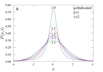
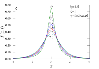
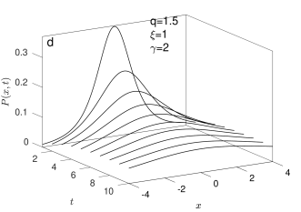
Figure 1: (a) L$q$-Gaussians for different $q$ values as indicated in the plot for $t=1,\xi=1,\gamma=2$ (b) L$q$-Gaussians for different $\xi$ values as indicated in the plot for $t=1,q=1.5,\gamma=2$ (c) L$q$-Gaussians for different $\gamma$ values as indicated in the plot for $t=1,q=1.5,\xi=1$ (d) Time evolution of the Green function of Eq. 6. Over time, the peak of curves decrease and the PDFs lost behavior of heavier tails, in contrast with (c), by increasing $\gamma,$ the peak of curves and behavior of heavier tails decrease.In (a), by increasing $q,$the peak of curves increase and the distribution becomes narrower (the tails become heavier).

III.2 A local fractional nonlinear time-space diffusion equation

In this section, we solved a time-space FPME (TS-FPME) with (LL) fractionalization. The Katugampola fractional definition was applied for the time and space fractional operators. Such FPME can be written as:

$$\begin{split}&\dfrac{\partial^{\xi}}{\partial t^{\xi}}P(x,t)=D\dfrac{\partial^{\gamma}}{\partial x^{\gamma}}P^{\nu}(x,t),\end{split}$$ (6)

where $0<\xi\leq 1<\gamma\leq 2,$ $|\nu|<1$ are a set of three free parameters, and $D$ is the diffusion coefficient. To solve Eq. (6), we express the function $P(x,t)$ in its self-similar form:

$$P(x,t)=\frac{1}{\phi(t)}F\left(\frac{x}{\phi(t)}\right),$$ (7)

where $\phi(t)$ is a function to be identified. The Eq. (7) is consistent with a symmetric probability distribution.

By considering, $z=\frac{x}{\phi(t)}$, and inserting Eq. (7) into Eq. (6), we have the following two equations:

$$\begin{split}&\partial^{\gamma}_{x}P^{\nu}=\frac{1}{\phi^{\nu+\gamma}}\frac{d^{\gamma}}{dz^{\gamma}}F^{\nu},\\ &\dfrac{\partial^{\xi}P}{\partial t^{\xi}}=\dfrac{-1}{\phi^{2}(t)}\dfrac{\partial^{\xi}\phi}{\partial t^{\xi}}\left[F+z\frac{d}{dz}F\right],\end{split}$$

so that,

$$\dfrac{-1}{\phi^{2}(t)}\dfrac{\partial^{\xi}\phi}{\partial t^{\xi}}\frac{d}{dz}[zF]=\dfrac{D}{\phi^{\nu+\gamma}}\frac{d^{\gamma}}{dz^{\gamma}}F^{\nu}.$$

In the above equation, the properties of the Katugampola derivative were used (see Appendix A and Table 4). Then, we arrange everything in such a way that all quantities in one side are only a function of $z$, and in the other side are a sole function of $t$. This procedure leads us to obtain the two following independent equations:

$$\begin{split}&\phi^{\nu+\gamma-2}\dfrac{\partial^{\xi}\phi}{\partial t^{\xi}}=\frac{\xi}{\nu+\gamma-1},\\ &-\dfrac{\xi}{\nu+\gamma-1}\frac{d}{dz}[zF]=D\frac{d^{\gamma}}{dz^{\gamma}}F^{\nu}.\end{split}$$

The solution of the first equation is $\phi\propto t^{\frac{\xi}{\nu+\gamma-1}},$ and for the second one we have:

$$\frac{d}{dz}[zF]=F+z\frac{d}{dz}F=k\frac{d^{\gamma}}{dz^{\gamma}}F^{\nu},$$

with $k=\frac{-D(\nu+\gamma-1)}{\xi}$, which can be rewritten as:

$$\frac{d}{dz}[zF]=k\frac{d^{\gamma-1}}{dz^{\gamma-1}}\frac{d}{dz}[F^{\nu}].$$ (8)

By applying the property: $\mathcal{D}^{\mu}(f)=\mathcal{D}^{\mu-1}\mathcal{D}^{1}(f)$ for $1<\mu\leqslant 2$, and taking local fractional integral with respect to $z$ in Eq. (8), the following expression is obtained:

$$\int^{t}\frac{d}{dz}[zF]\frac{dz}{z^{2-\gamma}}=k\int^{t}\frac{z^{2-\gamma}}{z^{2-\gamma}}\frac{d}{dz}\left[\frac{d}{dz}F^{\nu}\right]dz.$$ (9)

In the right hand side, the integration by parts is used, $\frac{z^{\gamma-1}F}{\gamma-1}+c$, choosing $c=0$. By considering $F=(c_{1}+c_{2}z^{\gamma})^{\frac{1}{\nu-1}}$ to obtain a special solution (where $c_{1}$ and $c_{2}$ are constants), the following expression is obtained:

$$\frac{d}{dz}[F^{\nu}]=\frac{\gamma\nu c_{2}}{\nu-1}z^{\gamma-1}F.$$

After incorporate the previous expression into the Eq. (9), we obtain:

$$c_{2}=\dfrac{-(\nu-1)\xi}{D\gamma(\gamma-1)\nu(\nu+\gamma-1)}.$$

Therefore, the general solution is:

$$P(x,t)\propto\frac{1}{t^{\frac{\xi}{\nu+\gamma-1}}}\left(c_{1}+\dfrac{(\nu-1)\xi}{D\gamma(\gamma-1)\nu(\nu+\gamma-1)}\frac{x^{\gamma}}{t^{\frac{\gamma\xi}{\nu+\gamma-1}}}\right)^{\frac{1}{\nu-1}},$$ (10)

where $c_{1}$ is removed after apply the normalization condition in Eq. (10). Then, by defining $\nu=2-q$, considering $\alpha=\frac{1-q+\gamma}{\xi}$, and

$$\begin{split}\eta^{L}_{q}(\xi,\gamma,q,D)&=\dfrac{\xi}{D\gamma(\gamma-1)\nu(\nu+\gamma-1)}\\ &=\dfrac{\xi}{D\gamma(\gamma-1)(2-q)(1-q+\gamma)},\end{split}$$ (11)

the following equation is reached:

$$P(x,t)=\frac{A^{L}_{q}}{t^{\frac{1}{\alpha}}}[1+(1-q)\eta^{L}_{q}(\beta,\gamma,q,D)\frac{x^{\gamma}}{t^{\frac{\gamma}{\alpha}}}]^{\frac{1}{1-q}},$$ (12)

where $A^{L}_{q}$ is a normalization factor. In most of physical systems cases, the $P(x,t)$ is symmetric with respect to $x$. This point leads us to make $x\rightarrow|x|$ (i.e. its absolute value), or we can consider some values of $\gamma$ that satisfy this property.
Then, the normalization factor was identified as follows:

$$A^{L}_{q}=\frac{1}{2}\left(\eta(\xi,\gamma,q,D)\right)^{\frac{1}{\gamma}}\dfrac{\Gamma(\frac{1}{q-1})}{\Gamma(\frac{1}{q-1}-\frac{1}{\gamma})\Gamma(1+\frac{1}{\gamma})},$$ (13)

where

$$\eta(\xi,\gamma,q,D)=\dfrac{\eta^{L}_{q}(\beta,\gamma,q,D)}{(\nu-1)^{-1}}.$$

For $\gamma=2$, these parameters become $\alpha=\frac{3-q}{\xi}$, $A^{L}_{q}=\sqrt{\pi^{-1}\eta(\xi,q,D)}\dfrac{\Gamma(\frac{1}{q-1})}{\Gamma(\frac{3-q}{2(q-1)})}$, and $\eta^{L}_{q}(\xi,q,D)=\dfrac{\xi}{2D(2-q)(3-q)}$.

We call Eq.(12) the local $q$-Gaussian (L$q$-Gaussian) distribution, which is the Green function of Eq.(6) obtained from a TS-FPME with the Katugampola fractional derivative (local fractional definition). The L$q$-Gaussian has been defined as, $g_{q}^{\gamma}(x)$, Equation N.$6$ in Table 2.

In Figure  1, we show the L$q$-Gaussians for different $q$ values as indicated in the plot for $t=1,\xi=1,\gamma=2$. In subfigure  1a, by increasing $q,$ the peak of curves increase and the distribution becomes narrower (the tails become heavier). In the case of subfigure 1b something similar occurs, where we denote the PDFs of L$q$-Gaussian for different $\xi$ values as indicated in the plot for $t=1,q=1.5$ and $\gamma=2$. The reverse occurs for Figure 1c, by increasing $\gamma$ (considering $t=1,q=1.5,\xi=1$), the peak of the PDFs decrease. Also, the time evolution of the Green function of Eq. 6 is shown in subfigure 1d.

III.3 A connection between the $(q,\alpha)$-stable distributions and L$q$-Gaussians

In the recent subsection, we obtained L$q$-Gaussian distributions by solving the TS-FPME. In fact, these L$q$-Gaussians are a generalized $q$-Gaussians by considering $|x|^{\gamma/2},\leavevmode\nobreak\ q>1$, i.e., a $q-$exponential in the variable $|x|^{\gamma}.$ From the definition of the $q$-exponential, it follows that $f\sim C_{f}|x|^{-\gamma/(q-1)},\,\,C_{f}>0,$ as $|x|\rightarrow\infty.$ Analogously, for any $q$-Gaussian, $g\sim C_{g}|x|^{-2/(q-1)},\,\,C_{g}>0,$ as $|x|\rightarrow\infty$. By comparing the order of the power law of the asymptotes, we verify that for a fixed $1<\gamma<2$, and for any $1<q<2$ there exists a proportionality from L$q$-Gaussians to $q$-Gaussian. For further details, see  Umarov .

Let us denote the class of random variables with $(q,\gamma)$-stable distributions by $\mathcal{L}_{q}[\gamma].$ A random variable $X\in\mathcal{L}_{q}[\gamma]$ has a symmetric density $f(x)$ with asymptotes $f\sim C|x|^{-(1+\gamma)/(1+\gamma(q-1))},\,|x|\rightarrow\infty,$ where $1\leq q<2,\,1<\gamma<2,$ and $C$ is a positive constant. On the other hand, any L$q$-Gaussian behaves asymptotically when $C_{1}/|x|^{\gamma/q-1}$. Especially any L$q_{\gamma}$-Gaussian behaves asymptotically when $C_{2}/|x|^{\gamma/(q_{\gamma}-1)}.$ Hence, we obtain the following relationship :

$$\dfrac{1+\gamma}{1+\gamma(q-1)}=\dfrac{\gamma}{q_{\gamma}-1}.$$ (14)

Solving this equation with respect to $q_{\gamma},$ we have

$$q_{\gamma}=\dfrac{\gamma Q_{\gamma}+1}{\gamma+1},\,\,\,Q_{\gamma}=2+\gamma(q-1).$$ (15)

Three parameters were linked: $\gamma,$ the parameter of the $\gamma$-stable Levy distributions, $q,$ the parameters of correlations, and $q_{\gamma},$ the parameters of attractors in terms of L$q_{\gamma}$-Gaussians. Then under Eq. (15) the density of $X\in\mathcal{L}_{q}[\gamma]$ is asymptotically equivalent to L$q_{\gamma}$-Gaussian.
The L$q$-Gaussians have an interesting property. Its successive derivatives, and integrations with respect to $|x|^{\gamma}$ correspond to $q_{\gamma,n}-$exponentials in the same variable $|x|^{\gamma}$, where $q_{\gamma,n}=\frac{\gamma q-n(q-1)}{\gamma-n(q-1)}$ Umarov .
By considering $\mathcal{G}_{q_{\gamma,n}}[\gamma]$ as a set of functions $\{be_{q_{\gamma,n}}^{-\beta|\xi|^{\gamma}},b>0,\beta>0\},$ and $\mathcal{F}_{q_{\gamma,n}}$ be the ${q_{\gamma,n}}-$Fourier transform, the following expression is obtained:

$$\mathcal{F}_{q_{\gamma,n}}:\mathcal{G}_{q_{\gamma,n}}[\gamma]\rightarrow\mathcal{G}_{q_{\gamma,n+1}}[\gamma],\,\,\,-\infty<n\leq[\gamma/(q-1)].$$

This is similar to the $q-$exponential with the variable $|\xi|^{\gamma}$, i.e. $e_{q}^{-\beta|\xi|^{\gamma}},\,\beta>0,$ which is the $q-$Fourier transform of $(q,\gamma)-$stable distributions Umarov .

III.4 The local fractional nonlinear time-space diffusion equation with the drift

The drift is often an inevitable part of stochastic systems , that should be analyzed in details for every case study to control its effects. Although it is suggested to define the equations for the general drift term. For the case where it depends only on time (as the case for many physical systems of interest), the situation becomes easier. In this case, the governing equation is:

$$\begin{split}\dfrac{\partial^{\xi}}{\partial t^{\xi}}&P(x,t)=-a(t)\dfrac{\partial P}{\partial x}+D\dfrac{\partial^{\gamma}P^{\nu}}{\partial x^{\gamma}},\\ &0<\xi\leq 1<\gamma\leq 2,\ \ |\nu|<1.\end{split}\,\,\,\,\,$$ (16)

By change of variable $\tau=t^{\xi}$ and the definition of the Katugampola derivative, we have:

$$\partial_{\tau}P=-a^{\prime}(\tau)\partial_{x}P+D\partial_{x}^{\gamma}P^{\nu},$$

where $a^{\prime}(\tau)=\frac{1}{\xi}a(t(\tau))$. By using the change of variable $(s,y)\equiv(\tau,x-x_{0}-f(\tau))$, where $f(\tau)=\int_{0}^{\tau}a^{\prime}(\tau^{\prime})d\tau^{\prime}$, and using the fact that $\frac{\partial y}{\partial\tau}=-a^{\prime}(\tau)$ and $\partial_{\tau}+a^{\prime}(\tau)\partial_{x}=\partial_{s}$, one finds that the governing equation $P(y,\tau)$ is:

$$\partial_{\tau}P(y,\tau)=D\partial_{y}^{\gamma}P^{\nu}(y,\tau),$$

for which the solution is $(x_{0}\equiv 0),$

$$P (y,\tau)=\frac{A}{\tau^{\frac{1}{1+\gamma-q}}}$$

$$\times(c_{1}-\dfrac{1-q}{2D\gamma(\gamma-1)(2-q)(1+\gamma-q)}\frac{y^{\gamma}}{\tau^{\frac{\gamma}{1+\gamma-q}}})^{\frac{1}{1-q}}.$$

Let us equate the $P(y,\tau)$:

$$P(x,t)=\frac{\partial{y}}{\partial{x}}P(y,\tau(t)).$$

Then, we obtain that:

$$P (x,t)=\frac{A}{t^{\frac{\xi}{1+\gamma-q}}}$$

$$\times\left(c_{1}-\dfrac{1-q}{2D\gamma(\gamma-1)(2-q)(1+\gamma-q)}\frac{(x-f^{\prime}(t))^{\gamma}}{t^{\frac{\gamma\xi}{1+\gamma-q}}}\right)^{\frac{1}{1-q}},$$ (17)

where $f^{\prime}(t)=f(\tau(t)),\,\,A$ is a normalization factor, and $c_{1}$ is a constant. The Eq. (17) is a L$q$-Gaussian solution with a drift.

IV PME with Local and Non-local Fractional Operators

To be self-contained, we consider the case where one fractional derivative is local, and the other is non-local. Therefore, in this section we solve a TS-FPME with (LN) fractionalization ,

$$\begin{split}&\dfrac{\partial^{\xi}}{\partial t^{\xi}}P(x,t)=D\dfrac{\partial^{\gamma}}{\partial x^{\gamma}}P^{\nu}(x,t),\\ &0<\xi\leq 1,\,\,0<\gamma<\frac{1}{2},\,\,\nu>-1,\end{split}$$ (18)

where $\dfrac{\partial^{\xi}}{\partial t^{\xi}}$ and $\dfrac{\partial^{\gamma}}{\partial x^{\gamma}}$ denote the Katugampola and Riemann-Liouville fractional derivatives, respectively (see Table 1). We consider the decomposition of (Eq. 7). Then, by using the property of $\frac{d^{\gamma}}{dx^{\gamma}}F(ax)=a^{\gamma}\frac{d^{\gamma}}{dz^{\gamma}}F(z)$, and some properties of Katugampola derivative we obtain:

$$\partial^{\gamma}_{x}P^{\nu}=\frac{1}{\phi^{\nu+\gamma}}\frac{d^{\gamma}}{dz^{\gamma}}F^{\nu},$$

$$\dfrac{\partial^{\xi}P}{\partial t^{\xi}}=\dfrac{-1}{\phi^{2}(t)}\dfrac{\partial^{\xi}\phi}{\partial t^{\xi}}\left[F+z\frac{d}{dz}F\right],$$

so that,

$$\dfrac{-1}{\phi^{2}(t)}\dfrac{\partial^{\beta}\phi}{\partial t^{\xi}}\frac{d}{dz}[zF]=\dfrac{D}{\phi^{\nu+\gamma}}\frac{d^{\gamma}}{dz^{\gamma}}F^{\nu}.$$

To continue, similar strategies applied in Sec. III.2 were used. We transform the previous equation into two independent equations:

$$\phi^{\nu+\gamma-2}\dfrac{\partial^{\xi}\phi}{\partial t^{\xi}}=\frac{\xi}{\nu+\gamma-1},$$

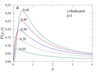
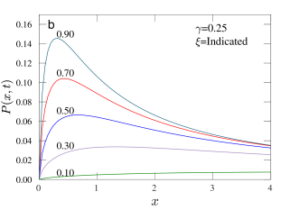
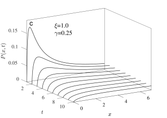
Figure 2: (a)The PDFs of the LNL$q$-Gaussian distributions for different values of $\gamma$ and $\xi=1$. (b)The PDFs of the LNL$q$-Gaussian distributions for different values of $\xi$ and $\gamma=0.25$. (c) Time evolution of the Green function of Eq. 18 .

$$-\dfrac{\xi}{\nu+\gamma-1}\frac{d}{dz}[zF]=D\frac{d^{\gamma}}{dz^{\gamma}}F^{\nu},$$

where the solution of the first equation is $\phi=t^{\frac{\xi}{\nu+\gamma-1}}$. For the second, the solution is :

$$\frac{d}{dz}[zF]=F+z\frac{d}{dz}F=-D\left[\frac{\nu+\gamma-1}{\xi}\right]\frac{d^{\gamma}}{dz^{\gamma}}F^{\nu},$$

or $\frac{d}{dz}[zF]=k\frac{d^{\gamma}}{dz^{\gamma}}F^{\nu}$ with $k=\frac{-D(\nu+\gamma-1)}{\xi}.$ By integrating with respect to $z,$ we obtain :

$$zF=k\frac{d^{\gamma-1}}{dz^{\gamma-1}}[F^{\nu}]+c,$$ (19)

where $c$ is a constant,we have set $c=0$. By considering $F(z)=z^{\mu}(c_{1}+c_{2}z)^{\lambda}$, and using the following property for the RL operators,

$$\mathcal{D}_{x}^{\delta}[x^{\alpha}(a+bx)^{\beta}]=a^{\delta}\dfrac{\Gamma(\alpha+1)}{\Gamma(\alpha+1-\delta)}x^{\alpha-\delta}(a+bx)^{\beta-\delta},$$ (20)

we find that

$$\frac{d^{\gamma-1}}{dz^{\gamma-1}}[F^{\nu}]=c_{1}^{\gamma-1}\frac{\Gamma(\nu\mu+1)}{\nu\mu+2-\gamma}z^{\nu\mu-\gamma+1}(c_{1}+c_{2}z)^{\nu\lambda-\gamma+1}.$$

We put this result into Eq.(19), and the following expressions are obtained:

$$\nu=\dfrac{2-\gamma}{1+\gamma},\,\,\mu=\dfrac{\gamma(1+\gamma)}{1-2\gamma},\,\,\lambda=\dfrac{1-\gamma^{2}}{2\gamma-1},$$

$$c_{1}^{\gamma-1}=\dfrac{-\beta(1+\gamma)\Gamma((2+\gamma(\gamma-3))(1-2\gamma)^{-1})}{D(1+\gamma(\gamma-1))\Gamma((1-\gamma^{2})(1-2\gamma)^{-1})}.$$

The recent expressions reveal that the master equation admits the following solution:

$$P(x,t)=\frac{A}{t^{\frac{1}{\sigma}}}\left(\frac{x}{t^{\frac{1}{\sigma}}}\right)^{\alpha\gamma}\left(c_{1}+c_{2}\frac{x}{t^{\frac{1}{\sigma}}}\right)^{-\alpha(1-\gamma)},$$ (21)

where $\alpha=\frac{1+\gamma}{1-2\gamma},\,\sigma=\frac{1-\gamma(1-\gamma)}{\beta(1+\gamma)},\,c_{2}=1$ and

$$A=\dfrac{\Gamma(\alpha(1-\gamma))}{c_{1}^{\gamma}\Gamma(1+\alpha\gamma)\Gamma(\gamma)}.$$

This solution is named local-non-local (LNL) $q$-Gaussian distribution. The solution is not a generalized $q$-Gaussian distribution. This occurs due to the factor, $x^{\alpha\gamma}$, which is located in front of the solution assuring that this class of PDFs tend to zero when $x\rightarrow 0$. This makes a great difference with the previous function, the L$q$-Gaussian Eq. (12).

Figure 2 shows the LNL$q$-Gaussian distribution functions. All the graphs tend to zero as $x\rightarrow 0$ for all times, as stated above, and don’t have symmetric form around their peaks in terms of $x$. They manifested an abrupt increase before the peak, and long-range tails beyond it, with peaks depending on $q$ and $\xi$. The peak values increase by increasing both $\gamma$ and $\xi$.

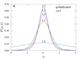
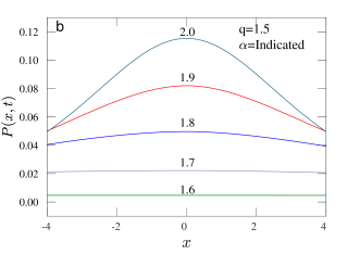
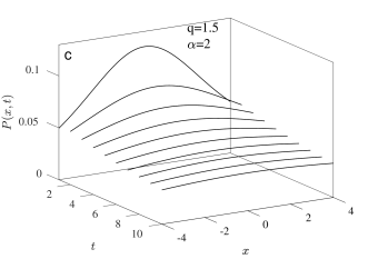
Figure 3: (a)The PDFs of the NL$q$-Gaussian distributions for $\alpha=2$ and indicated values of $q$ (b)The PDFs of the NL$q$-Gaussian distributions for $q=1.5$ and indicated value of $\alpha$. (c) The time evolution of PDFs of the NL$q$-Gaussian distributions for $q=1.5$ and $\alpha=2$. These are the Green functions of Eq. (22). We can see, the NL$q$-Gaussian for a constant value $\alpha$ and different $q$ values shows a multiple behavior; for $q=1.1,1.2,1.3$ the peak of curves and behavior of heavier tails increase, in contrast with $q=1.4,1.5.$ Also, for a constant value $q$ and different $\alpha$ values, by increasing $\alpha,$ the peak of curves and behavior of heavier tails increase. In time evolution of L$q$Gaussian, over time, the peak of curves decreases and the PDFs lost behavior of heavier tails.

V PME with Non-local Fractional Operators

In this section we solve one particular case of the G-PME displayed in Eq.(3), when $n=-1$, $a=0$, and $b=1$. The solution is obtained by considering a hybrid case, where the time derivative is RL operator, and the space derivative is Caputo operator (Appendix B). The other cases (RL-RL, Caputo-Caputo, and Caputo-RL derivatives) are straightforward to be processed following the same lines as this study. The resulting FPME equations is

$$_{0}\mathcal{D}^{\xi,\frac{1}{t}}P(x,t)=D\left({}^{C}\mathcal{D}_{1}^{\gamma,x^{\alpha}}P^{\nu}(x,t)\right),\,\,\,\,\,\,\,\xi,\gamma>0.$$ (22)

where $\mathcal{D}$ is the RL operator for time derivative and ${}^{C}\mathcal{D}$ is the Caputo operator acting on “space” coordinate $x$. To construct our solution, we need to restrict ourselves to the case $\nu=\frac{1+\xi}{1-\xi}$ leaving two parameters free for fitting, $\gamma$ and $\alpha$.

We again search for the solutions of the form of Eq. (7), where the parameters were defined in the Section III . In the following we show that the above equation admits the solution of the form $F(z)=(1+bz^{\alpha})^{\lambda}$, where $b\neq 0$, and $\alpha\neq 1$. When stablished, this solution serves as another variant of the generalized $q$-Gaussian solution. By inserting this form in the right side of Eq. (22) we obtain:

$${}^{C}\mathcal{D}_{1}^{\gamma,x^{\alpha}}P^{\nu}(x,t) = \left(\frac{1}{t^{\frac{1}{\alpha}}}\right)^{\nu}\leavevmode\nobreak\ \leavevmode\nobreak\ {}^{C}\mathcal{D}_{1}^{\gamma,x^{\alpha}}(1+bz^{\alpha})^{\lambda\nu}$$

$$=b^{\gamma}\left(\frac{1}{t}\right) {}^{\frac{\nu}{\alpha}+\gamma} \dfrac{\Gamma(\lambda\nu+1)}{\Gamma(\lambda\nu+1-\gamma)}(1+bz^{\alpha})^{\lambda\nu-\gamma}.$$ (23)

To obtain the above equation, we have used the following property of the fractional derivatives, that is valid for all the fractional differential operators considered here,

$$\mathcal{D}^{\mu}_{t}[f(at)]=a^{\mu}\mathcal{D}^{\mu}_{x}[f(x)]\mid_{x=at}.$$

Additionally, the following property of the fractional derivative of a function with respect to another function ref19 was applied :

$$\begin{split}\mathcal{D}_{b}^{\alpha,\psi}(\psi(b)-\psi(x))^{\beta-1}&=\dfrac{\Gamma(\beta)}{\Gamma(\beta-\alpha)}(\psi(b)-\psi(x))^{\beta-\alpha-1},\\ &\alpha>0,\,n<\beta\in\mathbb{R}.\end{split}$$ (24)

where $n=\alpha,$ if $\alpha\in\mathbb{N}$ and $n=[\alpha]+1,$ if $\alpha\notin\mathbb{N}.$
By inserting Eq. (7) in the left side of Eq. (22) and then applying Eq. (20) for the RL operators with $\delta=\alpha+\beta+1,$ we get

$${}_{0}\mathcal{D}^{\xi,\frac{1}{t}}P(x,t) = {}_{0}\mathcal{D}^{\xi,\frac{1}{t}}\{\frac{1}{t^{\frac{1}{\alpha}}}(1+bz^{\alpha})^{\lambda}\}$$

$$= {}_{0}\mathcal{D}^{\xi,\frac{1}{t}}\{\frac{1}{t^{\frac{1}{\alpha}}}(1+b^{\prime}\frac{1}{t})^{\lambda}\}$$

$$= \dfrac{\Gamma(\frac{1}{\alpha}+1)}{\Gamma(\frac{1}{\alpha}+1-\xi)} (1+bz^{\alpha})^{\lambda-\xi}\left(\frac{1}{t}\right)^{\frac{1}{\alpha}-\xi},$$ (25)

where $b^{\prime}=bx^{\alpha}$. By equating Eq. (V) and Eq. (V), one find that they match each other, yielding to:

$$\begin{split}&\xi=1+\lambda+1/\alpha,\nu=-1-\frac{2}{\lambda+1/\alpha},\\ &\gamma=(1/\alpha-\lambda)(1+\frac{1}{\lambda+1/\alpha}).\end{split}$$

Therefore, we see that the solution is:

$$P(x,t)=A^{NL}_{q}t^{\frac{-1}{\alpha}}\left[1+(1-q)\eta^{NL}_{q}(\alpha,\lambda,D)\frac{x^{\alpha}}{t}\right]^{\lambda},$$ (26)

where the pre-factor $A^{NL}_{q}$ is a normalization constant, and $\eta^{NL}_{q}(\alpha,\lambda,D)$ is a constant depending on $A^{NL}_{q}$. If we again suppose that the distribution is symmetric with respect to $x$. Therefore, $x\rightarrow|x|$ (i.e. its absolute value), then the normalization constant is:

$$A^{NL}_{q}=\frac{1}{2}\eta^{\frac{1}{\alpha}}(\alpha,\lambda,D)\dfrac{\Gamma(-\lambda)}{\Gamma(-\lambda-\frac{1}{\alpha})\Gamma(1+\frac{1}{\alpha})},$$

where $\eta(\alpha,\lambda,D)=\dfrac{\eta^{NL}_{q}(\alpha,\lambda,D)}{\lambda}$. From this expression one can calculate the final expression of $\eta^{NL}_{q}(\alpha,\lambda,D)$

$$\eta^{NL}_{q}(\alpha,\lambda,D)=...$$ (27)

$$... \lambda\left[2^{1-\nu}\alpha^{\nu}DB^{\nu}\left(-\lambda-\frac{1}{\alpha},\frac{1}{\alpha}\right)\Gamma(\lambda\nu+1)\Gamma\left(-\lambda-\frac{1}{\alpha}\right)\right]^{1/\xi},$$

where $B(.,.)$ is the Beta function. By defining $\lambda=\frac{1}{1-q}$ in Eq. (26) (where $q>1$), we recover the first generalized $q$-Gaussian distribution with two free independent parameters. We named Eq. (26) as the non- local $q$-Gaussian (NL$q$-Gaussian) distribution.
The NL$q$-Gaussian distribution Eq.(26) is the Green function of Eq.(22) obtained using the fractional derivatives of Riemann Liouville and Caputo, (non-local fractional definitions), for time and space, respectively. The NL$q$-Gaussian has been defined as $g_{q}^{\lambda,\alpha}(x)$, Equation N.$8$ in Table 2. The plots for NL$q$-Gaussian solutions are shown in Figure 3, for various $\alpha$ and $q$ values. With respect to the local case, the behavior for the non-local case is more complicated. As is seen from the subfigure 3a, the case where $\alpha$ is kept constant and $q$ increases is evaluated. For $q<1.3$, the peak rises, and for $q\geq 1.3$, it decreases. In subfigure 3b, for a constant $q$, however, the peak increases when $\alpha$ increases. The subfigure 3c shows the time evolution of the Green function of Eq. 22, which solution is the NL$q$-Gaussian distribution. The example was made for the values of $q=1.5$ and $\alpha=2$. We have shown that the distribution widens as time goes on.

VI AN Application of L$q$-Gaussian in S& P500 Stock Markets

The price return in stock markets exhibits remarkable characteristic features. The most largely observed feature in recent studies is the self similarity law , where the PDF obeys:

$$P(x,t)=\frac{1}{(Bt)^{H}}f\left(\dfrac{x}{(Bt)^{H}}\right),$$ (28)

	Classical (C-PME)	Time fractional (T-FPME)	Time-Space fractional (TS-FPME)	Particular case of the Generalized PME (G-PME )
Forms of PME	$\displaystyle\dfrac{\partial P}{\partial t}=$ $\displaystyle D\dfrac{\partial P^{2-q}}{\partial x^{2}},$ $\displaystyle 1<$ $\displaystyle q<3$	$\displaystyle\dfrac{\partial^{\xi}P(x,t)}{\partial t^{\xi}}=D$ $\displaystyle\dfrac{\partial^{2}P(x,t)^{2-q}}{\partial x^{2}},$ (29) $\displaystyle 0<\xi$ $\displaystyle\leq 1,$ (29) $\displaystyle 1<q$ $\displaystyle<3$ (29)	$\displaystyle\dfrac{\partial^{\xi}P}{\partial t^{\xi}}=D$ $\displaystyle\dfrac{\partial^{\gamma}P^{2-q}}{\partial x^{\gamma}},$ $\displaystyle 0<\xi$ $\displaystyle\leq 1,$ $\displaystyle 1<\gamma$ $\displaystyle\leq 2,$ $\displaystyle 1<q$ $\displaystyle<3$	$\displaystyle{}_{0}\mathcal{D}^{\xi,\frac{1}{t}}P=D$ $\displaystyle\left({}^{C}\mathcal{D}_{1}^{\gamma,x^{\alpha}}P^{\nu}\right),$ $\displaystyle\xi,\gamma$ $\displaystyle>0$
Parameters after comparing with General PME	$\begin{aligned} q&=2-\nu,\\ \gamma&=2,\\ \xi&=1\end{aligned}$	$\begin{aligned} q&=2-\nu,\\ \gamma&=2,\\ \xi&=\dfrac{3-q}{\alpha}\end{aligned}$	$\begin{aligned} q&=2-\nu,\\ \gamma&>1,\\ \xi&=\dfrac{1-q+\gamma}{\alpha}\end{aligned}$	$\begin{aligned} \xi&=1+\lambda+1/\alpha,\\ \nu&=-1-\frac{2}{\lambda+1/\alpha},\\ \gamma&=(1/\alpha-\lambda)\left(1+\frac{1}{\lambda+1/\alpha}\right)\end{aligned}$

Table 3: Summary of particular forms of the generalized PME Eq. 3 to model the time evolution of the PDFs of price return. The C-PME, T-FPME, TS-FPME and G-PME are obtained after set a specific value of the parameters in the general form of the PME. The fittings were perform by setting the parameters as shown in the table.

in which $f$ is a normalized distribution that is usually fit to a $q$-Gaussian ref8 . In earlier work, the function $f$ was assumed as a Levy-stable distribution function, $L_{\gamma}$, which has the drawback that it presents infinite standard deviation and it does not obey the empirical power law tails Gopi1998 ; Repe2004 .

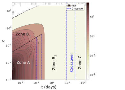
Figure 4: Three different zones were determined based on an abrupt slope change of the fitting parameters $\alpha$ and $q$. The contour plot represents the PDF of the detrended price return. The black circles represent the end points of the strong super-diffusion regime (zone A) from $t=0$ to $t=35$ minutes. These points are the ends of the bump obtained from the two points at the PDF with an abrupt change of slope (Figure 1-c in Alonso ). The remaining area during the first $35$ minutes corresponds to a weak super-diffusion regime (Zone $B_{1}$). From $80$ min to $10$ days, the zone corresponds to a weak super-diffusion regime (zone $B_{2}$). A normal diffusion process is reached after $30$ days. The gray dashed lines represent the transitions between each zone.

For long time returns it will be proved that $f$ is a Gaussian distribution function, where the price return behaves like independent and identically distributed random variables but still following the self similar principle. Particular cases of the generalized PME are presented in Table 3 . The solutions of each of these partial differential equations obey the self-similar law presented in Eq.(28) and are related to the q-Gaussian distribution function.

In this part, we analyze the S&P500 stock market data during the 24-year period from January 1996 to August 2020 with a frequency of one minute. The detrended price return is defined as,

$$x(t)=I^{*}(t_{o}+t)-I^{*}(t_{o}),$$ (30)

where $I^{*}(t_{o})$ is the detrended stock market index at time $t_{o}$, and $I^{*}(t)$ is the detrended stock market index for any time $t>t_{o}$. The PDF of the detrended price return has been fitted using the q-Gaussian distribution ref8 , where different zones had been captured from strong to super diffusion regime previously ref8 ; ref20 . Figure 4 shows the evolution of the PDF and its regimes in the $(x,t)$ space. Initially, the PDF has a pronounced bump in the center that fully disappears close to $80\,min$. During the first $35\,min$ there is a power law relation of time against the end points of the bumps at the PDFs (See Subfigure 1-e in Alonso ). This zone is defined as the strong super diffusion regime (Zone A). The remaining area during that time and the following next area close to $10$ days corresponds to the weak super diffusion regime (zone B). Finally, the last regime corresponds to a normal diffusion process (Zone C) and is reached after $30$ days approximately.

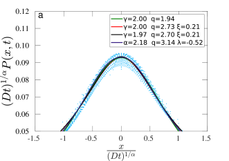
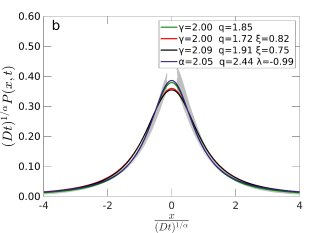
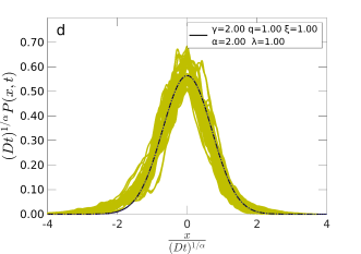
Figure 5: This figure shows the collapse of the time evolution of the PDFs for each zone displayed previously in Figure 4. (a) The collapse of the PDFs of the strong superdiffusion regime (Zone A), (b) The collapse of the PDFs of the weak superdiffusion regime for the first $35$ $min$ while the bump remains in the PDFs of Zone $B_{1}$. (c) The collapse of the PDF’s during the weak superdiffusion regime after $100$ $min$, when the bump disappears completely in Zone $B_{2}$, and (d) The collapse of the PDFs for the normal diffusion regime (Zone C). Each of the collapsed data is fitted by the solution of four different $q$-Gaussian forms, which are the solutions for the partial differential equations provided in Table I: no-fractional(green), time-fractional(red), time-space fractional (black), and a particular form of the G-PME (purple). For the subfigure (d) the collapsed data is fitted by a Gaussian distribution function, which is a concurrent solution for the four previous PDEs when $q=1$ and $\gamma=1$.

We have reconstructed the time evolution of the PDFs of the detrended price return and we collapsed them after applying the corresponding re-scaling factor. Four equations of the Table 2 have been used to model this behaviour. The Classical PME (C-PME), the time FPME (T-FPME), the time-space FPME (TS-FPME) and a particular case of the generalized PME (G-PME). These solutions obey Eq. (28), and are presented in Table 3 with more detail.

The TS-FPME and the particular solution of the G-PME proposed in this manuscript are new options to model the time evolution of the detrended price return. The L$q$-Gaussian and NL$q$-Gaussian, which are the solutions of the TS-FPME and the particular case of the G-PME respectively, fit the collapse of the PDFs of the detrended price return well. Figure 5 shows the result of these fittings.

The first best option to fit the price return was obtained by replacing $f$ as the L$q$-Gaussian ($g_{q}^{\gamma}$) in Eq. (28), this equation can be written as:

$$P(x,t)=\dfrac{1}{(Bt)^{\frac{\xi}{1-q+\gamma}}}\dfrac{1}{C_{q}^{\gamma}}{\left(1-(1-q)\dfrac{x^{\gamma}}{(Bt)^{\frac{\gamma\xi}{1-q+\gamma}}}\right)^{\dfrac{1}{1-q}}},$$ (31)

where $C_{q}^{\gamma}$ is the normalization constant. $B$ is related with the diffusion term, both of them are detailed in Table 2.

The second best option was obtained by replacing $f$ as the NL$q$-Gaussian ($g_{q}^{\alpha,\lambda}$) in Eq. (28), this second equation can be written as:

$$P(x,t)=\dfrac{1}{(Bt)^{\frac{1}{\alpha}}}\dfrac{1}{C_{q}^{\lambda,\alpha}}{\left(1-(1-q)\dfrac{x^{\alpha}}{(Bt)}\right)^{{\lambda}}}.$$ (32)

The $C_{q}^{\lambda,\alpha}$ is the normalization constant, and $B$ is related with the diffusion term. The definitions of these parameters are expressed in Table 2. By considering $\lambda=\dfrac{1}{1-q}$, the Eq. (31) is recovered.

The results of fitting the collapse of the PDF of the detrended price return are shown in Figure 5. The Figure 5 presents the collapses of the PDFs of price return for the specific zones presented in Figure 4. Each collapse has been fitted by the four solutions of the equations presented in Table 3. The best fitting for the four cases is the NL$q$-Gaussian. However, the four solutions constitutes an acceptable solution for the correspondent collapses of the PDFs. A converge to a Gaussian normal distribution is observed for long time returns.

VII Conclusions

We provided different solutions for the generalized form of the FPME. To this end, we had considered the generalized PME (G-PME) as the master equation. We introduced the anomalous PME as a nonlinear fractional diffusion equation, which is a particular case of G-PME. The solutions were built by considering the local and non-local fractional derivatives assuming a Dirac’s delta function as the initial condition. Our analysis proved that the solution are given by a generalized $q$-Gaussian, which obey a self similar law.
The fractional derivatives were classified as local and non-local, where the Katugampola’s is the local fractional derivative and the Riemman-Lioville, Caputo and Riesz are non-local fractional derivatives.
First, we considered the case where the derivatives are local. The resulting solution is L$q$-Gaussian, which is the first generalized $q$-Gaussian function. This solution fits the PDF of the detrended price return well (Sec. VI). The second analyzed class of G-PME is the one in which the time and space derivatives are given by the non-local fractional generalizations: Riemann-Lioville and Caputo, both of them based on the Laplace transform. For this second class, the fractional derivatives are evaluated with respect to another function, and proved that they admit the second generalized $q$-Gaussian solution. This second solution is symmetric about its mean (peak). The NL$q$-Gaussians hold a different self-similar law than the L$q$-Gaussians. The main difference is that the self-similarity of the L$q$-Gaussians depends on $\alpha$ and $\gamma$ only, for the NL$q$-Gaussians the self-similarity depends on $\alpha$, $\gamma$ and one extra global exponent $\lambda$, where the first generalized $q$-Gaussian is recover for $\lambda=\frac{1}{1-q}$. A hybrid equation has also been considered, where the time dimension is local fractional derivative, and the spatial dimension is non-local. The solution that we found is again proportional to the generalized $q$-Gaussian (which we named LNL$q$-Gaussian), but they obey a power in $x$ that causes the PDF to vanish in the limit $x\rightarrow 0$. The shape of these PDFs are very different from the $q$-Gaussian distribution and they are not symmetrical distribution.

The L$q$-Gaussian (first generalized q-Gaussian) and NL$q$-Gaussian (second generalized q-Gaussian) have been used to model the detrended price return of S&P500. Both distribution functions describe well the fitting of the detrended price return. The NL$q$-Gaussian is the best model to fit the probability of the detrended price return. For future work the generalized form of the PME will be solved by applying the $q$-Fourier analysis. The ordinary Fourier analysis only applies for linear operators. The generalized PME contains nonlinear operators, preventing us from using the ordinary Fourier analysis.

Appendix A Properties of Katugampola derivative

In here, we give a brief summary of the definition of the Katugampola fractional operator and some of its properties. This local fractional operator is used to construct the TS-FPME in sec. III. If $0\leq\alpha<1$, the Katugampola operator generalizes the classical calculus properties of polynomials Katugampola2014 . Furthermore, if $\alpha=1$, the definition is equivalent to the classical definition of the first order derivative of the function $f$. The Katugampola derivative is defined as:

$$\mathcal{D}^{\alpha}f(t)=\lim_{\epsilon\to 0}\dfrac{f(te^{\epsilon t^{-\alpha}})-f(t)}{\epsilon}$$ (33)

for $t>0$ and $\alpha\in(0,1]$. When $\alpha\in(n,n+1]$ (for some $n\in\mathbb{N}$, and $f$ is an $n-$differentiable at $t>0,$), the above definition generalizes to

$$\mathcal{D}^{\alpha}f(x)=\lim_{\epsilon\to 0}\dfrac{f^{(n)}(xe^{\epsilon x^{n-\alpha}})-f^{(n)}(x)}{\epsilon},$$

and if $f$ is $(n+1)-$differentiable at $t>0,$ then

$$\mathcal{D}^{\alpha}f(t)=t^{n+1-\alpha}f^{(n+1)}(t).$$

In continue, we review some properties of the Katugampola derivative in Table 4. If $f$ is $\alpha-$ differentiable in some $(0,a),\,a>0,$ and $f^{(\alpha)}(0)=\lim_{t\to 0^{+}}\mathcal{D}^{\alpha}f(t)$ exists, the following properties hold for Katugampola derivative. For $f,g$, be $\alpha-$ differentiable at a point $t>0.$

$$\mathcal{D}^{\alpha}f(at)= f^{\prime}(at)\mathcal{D}^{\alpha}(at)$$

$$=af^{\prime}(at)\mathcal{D}^{\alpha}t$$

$$=af^{\prime}(at)t^{1-\alpha}$$

$$=(at)^{1-\alpha}a^{\alpha}f^{\prime}(at).$$

One can define the inverse of the $\mathcal{D}^{\alpha}$ operator as a fractional integral,

$$(\mathcal{D}^{\alpha})^{-1}\equiv\mathcal{D}^{-\alpha}\equiv I^{\alpha}=\int^{t}dx\frac{(.)}{x^{1-\alpha}},$$

where the $(.)$ symbol is serving as place holder for the function to be operated upon. One verifies that

$$\mathcal{I}^{\alpha}[\mathcal{D}^{\alpha}(f)]=\int^{t}dx\frac{x^{1-\alpha}f^{\prime}}{x^{1-\alpha}}=f,$$

where $f$ vanishes at the lower limit. Then:

$$\mathcal{D}^{\alpha}[\mathcal{I}^{\alpha}(f)] =\mathcal{D}^{\alpha}[\int^{t}dx\frac{f}{x^{1-\alpha}}]$$

$$=t^{1-\alpha}\left(\int^{t}dt\frac{f}{x^{1-\alpha}}\right)^{\prime}$$

$$=t^{1-\alpha}\frac{f}{t^{1-\alpha}}=f.$$

Appendix B Caputo fractional derivative of a function with respect to another function

This section contains definitions of non-local fractional operators that are used in this paper to construct the TS-FPMEs. The Riemann-Liouville fractional derivative is a fractional operator that is used in Sections IV and  V as a non-local fractional operator to construct the TS-FPMEs with (LN) and (NN) fractionalizations. The integral representation for this operator is:

$${}^{RL}_{a}\mathcal{D}^{\alpha,x}f(t)=\frac{1}{\Gamma(n-\alpha)}\frac{d^{n}}{dx^{n}}\int_{a}^{x}\dfrac{dtf(t)}{(x-t)^{\alpha+1}},$$

where $n-1<\alpha\leq n$  ref21 . A recent variation of RL operator is the Caputo derivative Caputo , defined as:

$${}^{C}\mathcal{D}_{b}^{\alpha,x}f(t)=\frac{(-1)^{n}}{\Gamma(n-\alpha)}\int_{x}^{b}\dfrac{dtf^{(n)}(t)}{(x-t)^{\alpha+1-n}},\,\,\,\,\,n-1<\alpha\leq n,$$

where $C$ stands for Caputo and $f^{(n)}$ is the $n$th derivative of $f$. The main advantage of the Caputo derivative is that the derivate of a constant is zero, which is not the case of the RL operator. Substantially, this kind of fractional derivative is a formal generalization of the integer derivative under Laplace transform Bologna .

A generalized fractional operator that we used to construct the TS-FPME with (NN) fractionalization in Sec. V is the Caputo fractional derivative of a function with respect to another function ref19 , and defined as:

^C $$\mathcal{D}_{b}^{\alpha,\psi(x)}f(t)=\frac{(-1)^{n}}{\Gamma(n-\alpha)}...$$

$$...\times\int_{x}^{b}\psi(t)^{\prime}(\psi(t)-\psi(x))^{n-\alpha-1}(\frac{1}{\psi(t)^{\prime}}\frac{d}{dt})^{n}f(t)dt.$$

Note that the recent integral representation in the special case $\psi(x)=x$ is reduced to the integral representation of the Caputo derivative.
We solve a particular case of the generalized PME, Eq. (3), described by a fractional derivative of a function with respect to another function. This innovative approach will be useful to solve other physical problems that present a self-similar pattern and can be modelled by a $q$-Gaussian.

Appendix C Fractional derivatives: Definition and properties

In this section, we give a short review of the properties of the fractional derivatives: Katugampola, Riemann-Lioville, and Caputo. The Katugampola is one definition for the local fractional derivative. The Riemann-Lioville and Caputo are definitions of non-local derivatives. A comparison between each property of these fractional derivatives are presented in Table 4 .
Katugampola’s corresponds to the ordinary derivative when $\alpha=0$ and $\alpha=1$. The Riemann-Lioville and Caputo are an analytical continuation of the ordinary derivatives. The main difference between them is that the Caputo derivative of a constant is zero, a property that does not hold for Riemann-Lioville derivative. This desirable property is satisfied by the Katugampola local derivative, too.

Property	Katugampola Anderson2015 ; Katugampola2014	Riemann-Lioville Ishteva2005 ; Khader2015 ; He2012 ; ref19	Caputo Ishteva2005 ; Khader2015 ; He2012
Key Property	$\mathcal{D}^{\alpha}f(t)=\lim_{\epsilon\to 0}\dfrac{f(te^{\epsilon t^{-\alpha}})-f(t)}{\epsilon}$	${}^{RL}{\mathcal{D}}^{\alpha}f(t)={\mathcal{D}}^{n}{\mathcal{I}}^{n-\alpha}f(t)$	${}^{C}{\mathcal{D}}^{\alpha}f(t)={\mathcal{I}}^{n-\alpha}{\mathcal{D}}^{n}f(t)$
	$\mathcal{D}^{\alpha}f(t)=t^{1-\alpha}\dfrac{df(t)}{dt}$	$\quad\quad n-1<\alpha<n,\quad\quad{\mathcal{D}}^{n}=\dfrac{d^{n}}{dt^{n}},\,\,\,\,\quad\quad{\mathcal{I}}^{\alpha}f(t):=\dfrac{1}{\Gamma(\alpha)}\bigintss_{a}^{t}f(\tau)(t-\tau)^{\alpha-1}d\tau$
Cte. function	$\mathcal{D}^{\alpha}c=0$	${}^{RL}{\mathcal{D}}^{\alpha}c=\dfrac{c}{\Gamma(1-\alpha)}t^{-\alpha}$	${}^{C}{\mathcal{D}}^{\alpha}c=0$
Linearity	${\mathcal{D}}^{\alpha}(af(t)+g(t))=a{\mathcal{D}}^{\alpha}f(t)+\mathcal{D}^{\alpha}g(t)$
Product (Leibniz)	$\mathcal{D}^{\alpha}(f(t)g(t))=f(t)\mathcal{D}^{\alpha}g(t)+g(t)\mathcal{D}^{\alpha}f(t)$	${}^{RL}{\mathcal{D}}^{\alpha}(f(t)g(t))={\sum}_{k=0}^{\infty}\binom{\alpha}{k}(^{RL}\mathcal{D}^{\alpha-k}f(t))g^{k}(t)$	$\begin{aligned} {}^{C}{\mathcal{D}}^{\alpha}(f(t)g(t))=^{\,\,\,\,\,RL}{\mathcal{D}}^{\alpha}(f(t)g(t))....\\ ...-{\sum}_{k=0}^{n-1}\dfrac{t^{k-\alpha}}{\Gamma(k+1-\alpha)}((f(t)g(t))^{k}(0))\end{aligned}$
Quotient Rule	$\mathcal{D}^{\alpha}\left(\dfrac{f(t)}{g(t)}\right)=\dfrac{g(t)\mathcal{D}^{\alpha}f(t)-f(t)\mathcal{D}^{\alpha}g(t)}{g(t)^{2}}$
Chain Rule	$\mathcal{D}^{\alpha}\left(fog\right)=\dfrac{df}{dg}\mathcal{D}^{\alpha}g(t)$	$\begin{aligned} &{}^{RL}_{\,\,\,a}{\mathcal{D}}^{\alpha,x}(fog)=\\ &\dfrac{1}{\Gamma(1-\alpha)}\left(\dfrac{1}{g^{\prime}(x)}\dfrac{d}{dx}\right)^{n}\bigintss_{a}^{x}\dfrac{g^{\prime}(\tau)f(\tau)d\tau}{\left[g(x)-g(\tau)\right]^{1+\alpha-n}}\\ &{}^{RL}{\mathcal{D}}_{b}^{\alpha,x}(fog)=\\ &\dfrac{(-1)^{n}}{\Gamma(1-\alpha)}\left(\dfrac{1}{g^{\prime}(x)}\dfrac{d}{dx}\right)^{n}\bigintss_{x}^{b}\dfrac{g^{\prime}(\tau)f(\tau)d\tau}{\left[g(\tau)-g(x)\right]^{1+\alpha-n}}\end{aligned}$	$\begin{aligned} &{}^{C}_{\,\,\,a}{\mathcal{D}}^{\alpha,x}(fog)=\\ &\dfrac{1}{\Gamma(1-\alpha)}\bigintss_{a}^{x}\dfrac{g^{\prime}(\tau)f^{(n)}_{g}(\tau)d\tau}{\left[g(x)-g(\tau)\right]^{1+\alpha-n}},\\ &{}^{C}{\mathcal{D}}_{b}^{\alpha,x}(fog)=\\ &\dfrac{(-1)^{n}}{\Gamma(1-\alpha)}\bigintss_{x}^{b}\dfrac{g^{\prime}(\tau)f^{(n)}_{g}(\tau)d\tau}{\left[g(\tau)-g(x)\right]^{1+\alpha-n}},\\ &f_{g}^{n}(\tau)=\left(\dfrac{1}{g^{\prime}(x)}\dfrac{d}{dx}\right)^{n}f(\tau)\end{aligned}$
Power function	$\mathcal{D}^{\alpha}(t^{p})=pt^{p-\alpha}$	$\begin{aligned} {}^{\,\,\,RL}{\mathcal{D}}^{\alpha}(t^{p})&=\dfrac{\Gamma(p+1)}{\Gamma(p-\alpha+1)}t^{p-\alpha},\\ &p>-1,p\in\mathbb{R}\end{aligned}$	$\begin{aligned} {}^{C}{\mathcal{D}}^{\alpha}(t^{p})&=^{RL}{\mathcal{D}}^{\alpha}(t^{p}),\\ p>&n-1,p\in\mathbb{R}.\\ {}^{C}{\mathcal{D}}^{\alpha}(t^{p})&=0,\\ p\leqslant&n-1,p\in\mathbb{N}\end{aligned}$

Table 4: Comparison of properties between Katugampola, Riemman-Lioville and Caputo fractional derivatives.

References

- (1) Escobedo, M., Herrero, M. and Velazquez, J., 1998. A nonlinear Fokker-Planck equation modelling the approach to thermal equilibrium in a homogeneous plasma. Transactions of the American Mathematical Society, 350(10), pp.3837-3901.
- (2) Takai, M., Akiyama, H. and Takeda, S., 1981. Stabilization of drift-cyclotron loss-cone instability of plasmas by high frequency field. Journal of the Physical Society of Japan, 50(5), pp.1716-1722.
- (3) Spohn, H., 1993. Surface dynamics below the roughening transition. Journal de Physique I, 3(1), pp.69-81.
- (4) Marsili, M. and Bray, A.J., 1996. Soluble infinite-range model of kinetic roughening. Physical review letters, 76(15), p.2750.
- (5) Chavanis, P.H., 2006. Nonlinear mean-field Fokker–Planck equations and their applications in physics, astrophysics and biology. Comptes Rendus Physique, 7(3-4), pp.318-330.
- (6) Frank, T.D., 2005. Nonlinear Fokker-Planck equations: fundamentals and applications. Springer Science & Business Media.
- (7) FRANK, T. and BEEK, P., 2003. The Dynamical Systems Approach to Cognition: Concepts and Empirical Paradigms Based on Self-organization, Embodiment, and Coordination Dynamics, 10, p.159.
- (8) Wedemann, R.S. and Plastino, A.R., 2019, September. A Nonlinear Fokker-Planck Description of Continuous Neural Network Dynamics. In International Conference on Artificial Neural Networks (pp. 43-56). Springer, Cham.
- (9) Wedemann, R.S., Plastino, A.R. and Tsallis, C., 2016. Curl forces and the nonlinear Fokker-Planck equation. Physical Review E, 94(6), p.062105.
- (10) Plastino, A.R., Curado, E.M.F., Nobre, F.D. and Tsallis, C., 2018. From the nonlinear Fokker-Planck equation to the Vlasov description and back: Confined interacting particles with drag. Physical Review E, 97(2), p.022120.
- (11) Kozyreff, G., Vladimirov, A.G. and Mandel, P., 2000. Global coupling with time delay in an array of semiconductor lasers. Physical Review Letters, 85(18), p.3809.
- (12) Parrondo, J.M., Van den Broeck, C., Buceta, J. and de la Rubia, F.J., 1996. Noise-induced spatial patterns. Physica A: Statistical Mechanics and its Applications, 224(1-2), pp.153-161.
- (13) Okubo, A., 1980. Diffusion and ecological problems: mathematical models.
- (14) Ott, A., Bouchaud, J.P., Langevin, D. and Urbach, W., 1990. Anomalous diffusion in “living polymers”: A genuine Levy flight?. Physical review letters, 65(17), p.2201.
- (15) Ottinger, H.C., 2012. Stochastic processes in polymeric fluids: tools and examples for developing simulation algorithms. Springer Science & Business Media.
- (16) Bychuk, O.V. and O’Shaughnessy, B., 1995. Anomalous diffusion at liquid surfaces. Physical review letters, 74(10), p.1795.
- (17) Shiino, M., 1987. Dynamical behavior of stochastic systems of infinitely many coupled nonlinear oscillators exhibiting phase transitions of mean-field type: H theorem on asymptotic approach to equilibrium and critical slowing down of order-parameter fluctuations. Physical Review A, 36(5), p.2393.
- (18) Schwammle, V., Nobre, F.D. and Curado, E.M., 2007. Consequences of the H theorem from nonlinear Fokker-Planck equations. Physical Review E, 76(4), p.041123.
- (19) Frank, T.D., 2004. Autocorrelation functions of nonlinear Fokker-Planck equations. The European Physical Journal B-Condensed Matter and Complex Systems, 37(2), pp.139-142.
- (20) Wehner, M.F. and Wolfer, W.G., 1983. Numerical evaluation of path-integral solutions to Fokker-Planck equations. Physical Review A, 27(5), p.2663.
- (21) Borland, L., Pennini, F., Plastino, A.R. and Plastino, A., 1999. The nonlinear Fokker-Planck equation with state-dependent diffusion-a nonextensive maximum entropy approach. The European Physical Journal B-Condensed Matter and Complex Systems, 12(2), pp.285-297.
- (22) Ankudinova, J. and Ehrhardt, M., 2008. On the numerical solution of nonlinear Black–Scholes equations. Computers & Mathematics with Applications, 56(3), pp.799-812.
- (23) Barles, G. and Soner, H.M., 1998. Option pricing with transaction costs and a nonlinear Black-Scholes equation. Finance and Stochastics, 2(4), pp.369-397.
- (24) Alonso-Marroquin, F., Arias-Calluari, K., Harré, M., Najafi, M.N. and Herrmann, H.J., 2019. Q-Gaussian diffusion in stock markets. Physical Review E, 99(6), p.062313.
- (25) Barenblatt, G.I., Entov, V.M. and Ryzhik, V.M., 1989. Theory of fluid flows through natural rocks.
- (26) Michael, F. and Johnson, M.D., 2003. Financial market dynamics. Physica A: Statistical Mechanics and its Applications, 320, pp.525-534.
- (27) Borland, L., 2002. Option pricing formulas based on a non-Gaussian stock price model. Physical review letters, 89(9), p.098701.
- (28) Grandits, P., 2001. Frequent Hedging under Transaction Costs and a Nonlinear Fokker–Planck PDE. SIAM Journal on Applied Mathematics, 62(2), pp.541-562.
- (29) Zhang, D.S., Wei, G.W., Kouri, D.J. and Hoffman, D.K., 1997. Numerical method for the nonlinear Fokker-Planck equation. Physical review E, 56(1), p.1197.
- (30) Schwämmle, V., Curado, E.M. and Nobre, F.D., 2007. A general nonlinear Fokker-Planck equation and its associated entropy. The European Physical Journal B, 58(2), pp.159-165.
- (31) Martinez, S., Plastino, A.R. and Plastino, A., 1998. Nonlinear Fokker–Planck equations and generalized entropies. Physica A: Statistical Mechanics and its Applications, 259(1-2), pp.183-192.
- (32) Tsallis, C. and Lenzi, E.K., 2002. Anomalous diffusion: nonlinear fractional Fokker–Planck equation. Chemical Physics, 284(1-2), pp.341-347.
- (33) Frank, T.D., 2005. Nonlinear Fokker-Planck equations: fundamentals and applications. Springer Science & Business Media.
- (34) Carrillo, J.A., González, M.D.M., Gualdani, M.P. and Schonbek, M.E., 2013. Classical solutions for a nonlinear Fokker-Planck equation arising in computational neuroscience. Communications in Partial Differential Equations, 38(3), pp.385-409.
- (35) Caceres, M.J., Carrillo, J.A. and Tao, L., 2011. A numerical solver for a nonlinear Fokker–Planck equation representation of neuronal network dynamics. Journal of Computational Physics, 230(4), pp.1084-1099.
- (36) Aronson, D.G., 1986. The porous medium equation. In Nonlinear diffusion problems (pp. 1-46). Springer, Berlin, Heidelberg.
- (37) Quiros, F. and Vazquez, J.L., 1999. Asymptotic behaviour of the porous media equation in an exterior domain. Annali della Scuola Normale Superiore di Pisa-Classe di Scienze, 28(2), pp.183-227.
- (38) Gilding, B.H. and Peletier, L.A., 1976. On a class of similarity solutions of the porous media equation. Journal of mathematical analysis and applications, 55(2), pp.351-364.
- (39) Pamuk, S., 2005. Solution of the porous media equation by Adomian’s decomposition method. Physics Letters A, 344(2-4), pp.184-188.
- (40) Barbu, V., Da Prato, G. and Röckner, M., 2009. Existence of strong solutions for stochastic porous media equation under general monotonicity conditions. The Annals of Probability, 37(2), pp.428-452.
- (41) Barbu, V., Bogachev, V.I., Da Prato, G. and Röckner, M., 2006. Weak solutions to the stochastic porous media equation via Kolmogorov equations: the degenerate case. Journal of Functional Analysis, 237(1), pp.54-75.
- (42) Peletier, L.A., 1971. Asymptotic behavior of solutions of the porous media equation. SIAM Journal on Applied Mathematics, 21(4), pp.542-551.
- (43) Cordoba, D., Faraco, D. and Gancedo, F., 2011. Lack of uniqueness for weak solutions of the incompressible porous media equation. Archive for rational mechanics and analysis, 200(3), pp.725-746.
- (44) Angenent, S., 1988. Large time asymptotics for the porous media equation. In Nonlinear diffusion equations and their equilibrium states I (pp. 21-34). Springer, New York, NY.
- (45) Ganji, D.D. and Sadighi, A., 2007. Application of homotopy-perturbation and variational iteration methods to nonlinear heat transfer and porous media equations. Journal of Computational and Applied mathematics, 207(1), pp.24-34.
- (46) Bertsch, M. and Dal Passo, R., 1990. A numerical treatment of a superdegenerate equation with applications to the porous media equation. Quarterly of applied mathematics, 48(1), pp.133-152.
- (47) Duque, J.C., Almeida, R.M. and Antontsev, S.N., 2013. Convergence of the finite element method for the porous media equation with variable exponent. SIAM Journal on Numerical Analysis, 51(6), pp.3483-3504.
- (48) Macdonald, I.F., El-Sayed, M.S., Mow, K. and Dullien, F.A.L., 1979. Flow through porous media-the Ergun equation revisited. Industrial & Engineering Chemistry Fundamentals, 18(3), pp.199-208.
- (49) Ward, J.C., 1964. Turbulent flow in porous media. Journal of the hydraulics division, 90(5), pp.1-12.
- (50) Bologna, M., Tsallis, C. and Grigolini, P., 2000. Anomalous diffusion associated with nonlinear fractional derivative Fokker-Planck-like equation: Exact time-dependent solutions. Physical Review E, 62(2), p.2213.
- (51) Tsallis, C. and Bukman, D.J., 1996. Anomalous diffusion in the presence of external forces: Exact time-dependent solutions and their thermostatistical basis. Physical Review E, 54(3), p.R2197.
- (52) Drazer, G., Wio, H.S. and Tsallis, C., 2000. Anomalous diffusion with absorption: Exact time-dependent solutions. Physical Review E, 61(2), p.1417.
- (53) Compte, A. and Jou, D., 1996. Non-equilibrium thermodynamics and anomalous diffusion. Journal of Physics A: Mathematical and General, 29(15), p.4321.
- (54) Vazquez, J. L. (Juan Luis), The Porous Medium Equation Mathematical Theory . Oxford: Clarendon. Print.
- (55) Uchaikin, Vladimir V, Self-similar anomalous diffusion and Levy-stable laws, Physics-Uspekhi 46, no. 8 (2003): 821.
- (56) Bologna, M., Tsallis, C., & Grigolini, P. (2000), Anomalous diffusion associated with nonlinear fractional derivative Fokker-Planck-like equation: Exact time-dependent solutions. Physical Review E, 62(2), 2213.
- (57) Lenzi, E. K., Malacarne, L. C., Mendes, R. S., & Pedron, I. T. (2003). Anomalous diffusion, nonlinear fractional Fokker–Planck equation and solutions. Physica A: Statistical Mechanics and its Applications, 319, 245-252.
- (58) Bachelier, L. (1900), Théorie de la spéculation. In Annales scientifiques de l’École normale supérieure (Vol. 17, pp. 21-86).
- (59) Einstein, Albert, Investigations on the Theory of the Brownian Movement London: Methuen, 1926.
- (60) Mandelbrot, B. B. (1989), Louis Bachelier. In Finance (pp. 86-88). Palgrave Macmillan, London.
- (61) Levy, Paul, Théorie de l’addition des variables aléatoires, Gauthier-Villars, Paris, 1937. LévyThéorie de l’addition des variables aléatoires1937 (1954).
- (62) Feller, William, On a generalization of Marcel Riesz’potentials and the semi-groups generated by them, Gleerup, 1962.
- (63) Gorenflo, Rudolf, Gianni De Fabritiis, and Francesco Mainardi,Discrete random walk models for symmetric Lévy–Feller diffusion processes. Physica A: Statistical Mechanics and its Applications 269, no. 1 (1999): 79-89.
- (64) Xu, Yong, Wanrong Zan, Wantao Jia, and Jürgen Kurths, Path integral solutions of the governing equation of SDEs excited by Lévy white noise. Journal of Computational Physics 394 (2019): 41-55.
- (65) Janakiraman, Deepika, and K. L. Sebastian, Path-integral formulation for Lévy flights: Evaluation of the propagator for free, linear, and harmonic potentials in the over-and underdamped limits. Physical Review E 86, no. 6 (2012): 061105.
- (66) Barenblatt, G. I, On self-similar motions of compressible fluids in porous media. Prikl. Math. (1952): 679-698.
- (67) Esteban, Juan R., and Juan L. Vázquez. , On the equation of turbulent filtration in one-dimensional porous media. Nonlinear Analysis: Theory, Methods & Applications 10, no. 11 (1986): 1303-1325.
- (68) Tsallis, C. (2005), Nonextensive statistical mechanics, anomalous diffusion and central limit theorems. Milan Journal of Mathematics, 73(1), 145-176.
- (69) Plastino, A. R., and A. Plastino, Non-extensive statistical mechanics and generalized Fokker-Planck equation. Physica A: Statistical Mechanics and its Applications 222, no. 1-4 (1995): 347-354.
- (70) Tsallis, Constantino, and Dirk Jan Bukman, Anomalous diffusion in the presence of external forces: Exact time-dependent solutions and their thermostatistical basis. Physical Review E 54, no. 3 (1996): R2197.
- (71) Umarov, S., Tsallis, C. and Steinberg, S., 2008. On a q-central limit theorem consistent with nonextensive statistical mechanics. Milan journal of mathematics, 76(1), pp.307-328.
- (72) Tsallis, C. and Duarte Queirós, S.M., 2007, December. Nonextensive statistical mechanics and central limit theorems I—Convolution of independent random variables and q‐product. In AIP Conference Proceedings (Vol. 965, No. 1, pp. 8-20). American Institute of Physics.
- (73) Jain, R. and Sebastian, K.L., 2017. Lévy flight with absorption: a model for diffusing diffusivity with long tails. Physical Review E, 95(3), p.032135.
- (74) Arias-Calluari, K., Alonso-Marroquin, F. and Harré, M.S., 2018. Closed-form solutions for the Lévy-stable distribution. Physical Review E, 98(1), p.012103.
- (75) G.Sales Teodoro, J.A.Tenreiro Machado, and E.Capelas de Oliveira, A review of definitions of fractional derivatives and other operators, Journal of Computational Physics, Volume 388, 1 July 2019, P. 195-208, https://doi.org/10.1016/j.jcp.2019.03.008.
- (76) M. Bologna, C. Tsallis, P. Grigolini, Anomalous diffusion associated with nonlinear fractional derivative Fokker–Planck-like equation: exact time-dependent solutions Phys Rev E, 62 (2000), p. 2213-2218.
- (77) E.K. Lenzi, G.A. Mendes, R.S. Mendes, L.R. Silva, L.S. Lucena, Exact solutions to nonlinear non autonomous space-fractional diffusion equations with absorption, Phys. Rev. E, 67 (2003), p. 051109.
- (78) E.K. Lenzi, R.S. Mendes, K.S. Fa, L.S. Moraes, L.R. Silva, L.S. Lucena, Nonlinear fractional diffusion equation: exact results, J. Math. Phys., 46 (2005), p. 083506.
- (79) P.C. Assis, L.R. Silva, E.K. Lenzi, L.C. Malacarne, R.S. Mendes, diffusion equation, Tsallis formalism and exact solutions, J. Math. Phys., 46 (2005), p. 123-303.
- (80) A.T. Silva, E.K. Lenzi, L.R. Evangelista, M.K. Lenzi, LRda Silva, Fractional nonlinear diffusion equation, solutions and anomalous diffusion, Physica A, 375 (2007), p. 65-71.
- (81) E.K. Lenzi, M.K. Lenzi, L.R. Evangelista, L.C. Malacarne, R.S. Mendes, Solutions for a fractional nonlinear diffusion equation with external force and absorbent term, J. Stat. Mech. (2009), p. P02048.
- (82) F. Alonso-Marroquin, K.Arias-Calluari, M. Harré, M. N. Najafi, and H. J. Herrmann, Q-Gaussian diffusion in stock markets, PHYSICAL REVIEW E 99, 062313 (2019), DOI: 10.1103/PhysRevE.99.062313.
- (83) J. L. Vazquez, The Porous Medium Equation: Mathematical Theory (Clarendon, Oxford, 2007).
- (84) W. Chen, Fractional and fractal derivatives modeling of turbulence, J. Am. Math. Soc. (2014), arXiv:1410.6535.
- (85) W. Chen, Time-space fabric underlying anomalous diffusion, Chaos Solitons Fractals 28 (2006), p. 923-929.
- (86) R. Khalil, M.A. Horani, A. Yousef, M. Sababheh, A new definition of fractional derivative, J. Comput. Appl. Math. 264 (2014), p. 65-70.
- (87) W.S. Chung, Fractional Newton mechanics with conformable fractional derivative, J. Comput. Appl. Math. 290 (2015), p. 150-158.
- (88) B.B.I. Eroglu, D. Avci, N. Ozdemir, Optimal control problem for a conformable fractional heat conduction equation, Acta Phys. Pol. A 132 (2017), p. 658-662.
- (89) B. Bayour, D.F.M. Torres, Existence of solution to a local fractional nonlinear differential equation, J. Comput. Appl. Math. 312 (2017), p.127-133.
- (90) F. Zulfeqarr, A. Ujlayan, P. Ahuja A new fractional derivative and its fractional integral with some applications, arXiv:1705 .00962v1, 2017.
- (91) U.N. Katugampola, A new fractional derivative with classical properties, J. Am. Math. Soc. (2014), arXiv:1410.6535. arXiv:nlin /0511066v1, IAPCM Report, 2005.
- (92) M. Bologna, Derivative of Real Index, (Edizioni Tecnico Scientifiche, Pisa, 1990) (in Italian)
- (93) R. Almeida, A Caputo fractional derivative of a function with respect to another function, Communications in Nonlinear Science and Numerical Simulation, 44 (2017), P. 460-481
- (94) K. Arias-Calluari, F. Alonso-Marroquin, M. N. Najafi, and M. Harré, Forecasting the effect of COVID-19 on the S&P500, archivePrefix-q-fin.ST. eprint=2005.03969 (2020)
- (95) K.S. Miller, B. Ross An introduction to the fractional calculus and fractional differential equations, John Wiely & Sons, New York, NY, USA, 1993.
- (96) R. Almeida, M.Guzowska, T. Odzijewicz A remark on local fractional calculus and ordinary derivatives, Open Mathematics, 14 (2016), P. 1122–1124.
- (97) A. A. Kilbas, H. M. Srivastava , J.J. Trujillo, Theory and Applications of Fractional Differential Equations. North-Holland Mathematics Studies, 204. Elsevier Science B.V., Amsterdam, 2006.
- (98) M. Caputo, Elasticita‘ e dissipazione. (Zanichelli, Bologna, 1969); M. Caputo and F. Mainardi, Riv. Nuovo Cimento, 1, 161 (1971).
- (99) S. Umarov, C. Tsallis, M. Gell-Mann, S. Steinberg, Generalization of symmetric stable Lévy distributions for . J. Math. Phys. 51, 033502 (2010).
- (100) Gopikrishnan, Parameswaran, Martin Meyer, LA Nunes Amaral, and H. Eugene Stanley, Inverse cubic law for the distribution of stock price variations, The European Physical Journal B-Condensed Matter and Complex Systems 3, no. 2 (1998): 139-140.
- (101) Repetowicz, Przemyslaw, and Peter Richmond, Modeling of waiting times and price changes in currency exchange data, Physica A: Statistical Mechanics and its Applications 343 (2004): 677-693.
- (102) Anderson, Douglas R., and Darin J. Ulness, Properties of the Katugampola fractional derivative with potential application in quantum mechanics, Journal of Mathematical Physics 56, no. 6 (2015): 063502.
- (103) Mainardi, Francesco, M. U. R. A. Antonio, Gianni Pagnini, and Rudolf Gorenflo, Fractional relaxation and time-fractional diffusion of distributed order. IFAC Proceedings Volumes 39, no. 11 (2006): 1-21.
- (104) Yang, Xiao-Jun, General Fractional Derivatives: Theory, Methods, and Applications Boca Raton. CRC Press, Taylor & Francis Group, 2019,isbn 9780429284083.
- (105) Uchaikin, Vladimir V, Albert C. J Luo, and Nail H Ibragimov, Fractional Derivatives for Physicists and Engineers: Background and Theory. Berlin, Heidelberg: Springer Berlin Heidelberg, 2013,isbn,9783642339103.
- (106) Gorenflo, Rudolf, and Francesco Mainardi, Fractional calculus and stable probability distributions. Archives of Mechanics 50, no. 3 (1998): 377-388.
- (107) Gorenflo, Rudolf, Francesco Mainardi, Daniele Moretti, Gianni Pagnini, and Paolo Paradisi, Discrete random walk models for space–time fractional diffusion. Chemical physics 284, no. 1-2 (2002): 521-541.
- (108) Sun, Zhaopeng, Hao Dong, and Yujun Zheng, Fractional dynamics using an ensemble of classical trajectories.Physical Review E 97, no. 1 (2018): 012132.
- (109) Celik, Cem, and Melda Duman, Crank–Nicolson method for the fractional diffusion equation with the Riesz fractional derivative.Journal of computational physics 231, no. 4 (2012): 1743-1750.
- (110) Katugampola, Udita N,A new fractional derivative with classical properties. arXiv preprint arXiv:1410.6535 (2014).
- (111) Ishteva, M., Properties and applications of the Caputo fractional operator. Department of Mathematics, University of Karlsruhe, Karlsruhe 5 (2005).
- (112) Khader, M. M.,An efficient approximate method for solving fractional variational problems. Applied Mathematical Modelling 39, no. 5-6 (2015): 1643-1649.
- (113) He, Ji-Huan, S. K. Elagan, and Z. B. Li,Geometrical explanation of the fractional complex transform and derivative chain rule for fractional calculus.Physics letters A 376, no. 4 (2012): 257-259.