A [akema@sp.ce.titech.ac.jp]Riku AkemasTokyoTech1808273 [myamagi@sp.ce.titech.ac.jp]Masao YamagishimTokyoTech0903663 [isao@sp.ce.titech.ac.jp]Isao YamadafTokyoTech8510504 [TokyoTech]The author is with the Department of Information and Communications Engineering, Tokyo Institute of Technology 2-12-1-S3-60 Ookayama, Meguro-ku, Tokyo 152-8550, Japan. 510 97

Approximate Simultaneous Diagonalization of Matrices via Structured Low-Rank Approximation

Approximate Simultaneous Diagonalization (ASD) is a problem to find a common similarity transformation which approximately diagonalizes a given square-matrix tuple. Many data science problems have been reduced into ASD through ingenious modelling. For ASD, the so-called Jacobi-like methods have been extensively used. However, the methods have no guarantee to suppress the magnitude of off-diagonal entries of the transformed tuple even if the given tuple has a common exact diagonalizer, i.e., the given tuple is simultaneously diagonalizable. In this paper, to establish an alternative powerful strategy for ASD, we present a novel two-step strategy, called Approximate-Then-Diagonalize-Simultaneously (ATDS) algorithm. The ATDS algorithm decomposes ASD into (Step 1) finding a simultaneously diagonalizable tuple near the given one; and (Step 2) finding a common similarity transformation which diagonalizes exactly the tuple obtained in Step 1. The proposed approach to Step 1 is realized by solving a Structured Low-Rank Approximation (SLRA) with Cadzow’s algorithm. In Step 2, by exploiting the idea in the constructive proof regarding the conditions for the exact simultaneous diagonalizability, we obtain a common exact diagonalizer of the obtained tuple in Step 1 as a solution for the original ASD. Unlike the Jacobi-like methods, the ATDS algorithm has a guarantee to find a common exact diagonalizer if the given tuple happens to be simultaneously diagonalizable. Numerical experiments show that the ATDS algorithm achieves better performance than the Jacobi-like methods.

1 Introduction

One of the most important tasks in data sciences is to extract certain common features from given multiple data [1, 2]. Many approaches [3, 4, 5, 6, 7, 8, 9, 10, 11, 12, 13] reduce such tasks into a problem to find a common similarity transformation which diagonalizes simultaneously a certain matrix tuple observed under the influence of noise. A matrix tuple is called in this paper a simultaneously diagonalizable tuple (see Definition 1) if it has a common similarity transformation which diagonalizes exactly all matrices in the tuple. Let ${\mathfrak{D}^{\mathrm{abl}}_{n,K}}$ be the set of all simultaneously diagonalizable tuples in ${\mathbb{C}^{n\times n}}\times{\mathbb{C}^{n\times n}}\times\cdots\times{\mathbb{C}^{n\times n}}\eqqcolon{\bigtimes_{k=1}^{K}}{\mathbb{C}^{n\times n}}$ (see Definition 1 for the precise definition of ${\mathfrak{D}^{\mathrm{abl}}_{n,K}}$ and A for the nonconvexity of ${\mathfrak{D}^{\mathrm{abl}}_{n,K}}$). For a given ${\mathbf{A}}=(A_{1},\ldots,A_{K})\in{\mathfrak{D}^{\mathrm{abl}}_{n,K}}$, the exact simultaneous diagonalization requires to find $S\in{\mathbb{C}^{n\times n}}$ such that $S^{-1}A_{k}S\ (k=1,\ldots,K)$ are diagonal. In this paper, for a general ${\mathbf{A}}\in{\bigtimes_{k=1}^{K}}{\mathbb{C}^{n\times n}}$, we consider the following problem.

Problem 1 (Approximate Simultaneous Diagonalization: ASD).

For a given ${\mathbf{A}}=(A_{1},A_{2},\ldots,A_{K})\in{\bigtimes_{k=1}^{K}}{\mathbb{C}^{n\times n}}$, approximate ${\mathbf{A}}$ with a certain ${\tilde{{\mathbf{A}}}}=({\tilde{A}}_{1},\ldots,{\tilde{A}}_{K})\in{\mathfrak{D}^{\mathrm{abl}}_{n,K}}$ and find ${\tilde{S}}\in{\mathbb{C}^{n\times n}}$ such that ${\tilde{S}}^{-1}{\tilde{A}}_{k}{\tilde{S}}\ (k=1,\ldots,K)$ are diagonal.

A conventional nonconvex optimization model for the ASD of ${\mathbf{A}}=(A_{1},\ldots,A_{K})\in{\bigtimes_{k=1}^{K}}{\mathbb{C}^{n\times n}}$ is to find a minimizer of $f_{\mathbf{A}}(S)\coloneqq\sum_{k=1}^{K}{\operatorname{off}}(S^{-1}A_{k}S)$, where ${\operatorname{off}}\colon[x_{i,j}]_{i,j=1}^{n}\mapsto\sum_{1\leq i\neq j\leq n}\left\lvert x_{i,j}\right\rvert^{2}$. For this optimization model, the so-called Jacobi-like methods have been used extensively [14, 15, 5, 10]. Although such methods can be applied directly to general matrix tuples, they can update only few variables in an estimate of a minimizer of $f_{\mathbf{A}}$ with certain parameterized matrices, e.g., the Givens rotation matrices and the shearing matrices. More importantly, the Jacobi-like methods have no guarantee to suppress $f_{\mathbf{A}}$ even for ${\mathbf{A}}\in{\mathfrak{D}}^{\mathrm{abl}}_{2,2}$ (see Example 1 in Section 2.2 for its details). On the other hand, the idea found in the constructive proof for a classical relation between diagonalizability and commutativity (see Fact 2) regarding the exact simultaneous diagonalizability suggests that we can solve the exact simultaneous diagonalization for ${\mathbf{A}}\in{\mathfrak{D}^{\mathrm{abl}}_{n,K}}$ algebraically (Note: such an exact simultaneous diagonalization along this idea is found as, e.g., Diagonalize-One-then-Diagonalize-the-Other (DODO) method in [16]; see Algorithm 1 in Section 2.2). This situation suggests the possibility to establish a new powerful strategy which can supersede the Jacobi-like methods for ASD if a simultaneously diagonalizable tuple can be found as a good approximation of ${\mathbf{A}}\in{\bigtimes_{k=1}^{K}}{\mathbb{C}^{n\times n}}$.

In this paper, to establish such a computational scheme, we present a novel two-step strategy, named Approximate-Then-Diagonalize-Simultaneously (ATDS) algorithm, as a practical solution of the following problem.

Problem 2 (Two steps for approximate simultaneous diagonalization).

For a given ${\mathbf{A}}\in{\bigtimes_{k=1}^{K}}{\mathbb{C}^{n\times n}}$,

Step 1 (Approximation):

approximate ${\mathbf{A}}$ with a certain ${\tilde{{\mathbf{A}}}}=({\tilde{A}}_{1},\ldots,{\tilde{A}}_{K})\in{\mathfrak{D}^{\mathrm{abl}}_{n,K}}$, where ${\tilde{{\mathbf{A}}}}={\mathbf{A}}$ must be employed if ${\mathbf{A}}\in{\mathfrak{D}^{\mathrm{abl}}_{n,K}}$;

Step 2 (Simultaneous diagonalization):

find a common exact diagonalizer of ${\tilde{{\mathbf{A}}}}=({\tilde{A}}_{1},\ldots,{\tilde{A}}_{K})$, i.e., find ${\tilde{S}}\in{\mathbb{C}^{n\times n}}$ s.t. ${\tilde{S}}^{-1}{\tilde{A}}_{k}{\tilde{S}}\ (k=1,\ldots,K)$ are diagonal.

Since Step 2 can be solved by the DODO method, we focus on Step 1. The proposed approach to Step 1 is designed based on the fact that a necessary condition for ${\mathbf{X}}\in{\mathfrak{D}^{\mathrm{abl}}_{n,K}}$ can be translated into a certain rank condition for a structured matrix defined with ${\mathbf{X}}$ (see Theorem 1). More precisely, we propose to relax Step 1 by Step 1’ with Structured Low-Rank Approximation (SLRA) [17] and then propose to solve Step 1’ with Cadzow’s algorithm [18]. Unlike the Jacobi-like methods, the proposed ATDS algorithm has a guarantee to find a common exact diagonalizer if ${\mathbf{A}}$ happens to satisfy ${\mathbf{A}}\in{\mathfrak{D}^{\mathrm{abl}}_{n,K}}$. Numerical experiments show that, compared with the Jacobi-like methods, the proposed ATDS algorithm achieves a better approximation to the desired common similarity transformation at the expense of reasonable computational time.

A preliminary version of this paper was presented at a conference [19].

Notations (see also Table 1). Let ${\mathbb{N}}$, ${\mathbb{R}}$, and ${\mathbb{C}}$ denote the set of all nonnegative integers, the set of all real numbers, and the set of all complex numbers, respectively. For ${\mathbf{x}}\in{\mathbb{C}}^{n}$, $\|{\mathbf{x}}\|$ denotes the Euclidean norm of ${\mathbf{x}}$. The matrix $I_{n}$ denotes the $n$-by-$n$ identity matrix. For $X\in{\mathbb{C}^{m\times n}}$, $X^{\top}$, $X^{\ast}$, $X^{-1}$, $X^{-\top}$, ${\operatorname{tr}}(X)$, $\|X\|_{F}$, ${\operatorname{range}}(X)$, and ${\operatorname{nullspace}}(X)$ denote respectively the transpose, the conjugate transpose, the inverse, the inverse of transpose, the trace, the Frobenius norm, the range space, and the nullspace of $X$. The mapping ${\operatorname{vec}}:{\mathbb{C}^{m\times n}}\rightarrow{\mathbb{C}}^{mn}$ denotes vectorization by stacking the columns of a matrix and ${\operatorname{vec}}^{-1}$ its inverse. For ${\mathbf{x}}\in{\mathbb{C}^{n}}$, ${\operatorname{diag}}({\mathbf{x}})\in{\mathbb{C}^{n\times n}}$ is a diagonal matrix whose diagonal entries are given by the components of ${\mathbf{x}}$. The Kronecker product of $X=[x_{i,j}]\in{\mathbb{C}^{m\times n}}$ and $Y\in{\mathbb{C}}^{p\times q}$ is $X\otimes Y\in{\mathbb{C}}^{mp\times nq}$ whose $(i,j)$th blocks are $[X\otimes Y]_{i,j}=x_{i,j}Y\ (i=1,2,\ldots,m;j=1,2,\ldots,n)$. The Khatri-Rao product of $X=[{\mathbf{x}}_{1}\ \cdots\ {\mathbf{x}}_{l}]\in{\mathbb{C}}^{m\times l}$ and $Y=[{\mathbf{y}}_{1}\ \cdots\ {\mathbf{y}}_{l}]\in{\mathbb{C}}^{n\times l}$ is $X\odot Y\coloneqq[{\mathbf{x}}_{1}\otimes{\mathbf{y}}_{1}\ \cdots\ {\mathbf{x}}_{l}\otimes{\mathbf{y}}_{l}]\in{\mathbb{C}}^{mn\times l}$. The direct sum of $\check{X}_{p}\in{\mathbb{C}}^{n_{p}\times n_{p}}\ (p=1,\ldots,d;n_{1}+\cdots+n_{d}=n)$ is the block diagonal matrix $\check{X}_{1}\oplus\check{X}_{2}\oplus\cdots\oplus\check{X}_{d}\in{\mathbb{C}^{n\times n}}$ with the $i$th diagonal block $\check{X}_{i}~{}(i=1,\ldots,d)$. For $X_{p}\in{\mathbb{C}}^{m\times n}\ (p=1,\ldots,d)$, ${\operatorname{span}}\{X_{1},\ldots,X_{d}\}\subset{\mathbb{C}}^{m\times n}$ is the set of all linear combinations of $X_{1},\ldots,X_{d}$. For ${\mathbf{X}}=(X_{1},\ldots,X_{K})\in{\bigtimes_{k=1}^{K}}{\mathbb{C}^{n\times n}}$, we define ${\left\lVert{\mathbf{X}}\right\rVert}_{F}\coloneqq\sqrt{\sum_{k=1}^{K}{\left\lVert X_{k}\right\rVert}_{F}^{2}}$.

2 Preliminaries

2.1 Useful Facts on Diagonalizability

Recall that $X\in{\mathbb{C}^{n\times n}}$ is said to be diagonalizable if there exists $S\in{\mathbb{C}^{n\times n}}$ such that $S^{-1}XS$ is diagonal. In the following, we use ${\mathsf{D}^{\mathrm{abl}}_{n}}\subset{\mathbb{C}^{n\times n}}$ to denote the set of all diagonalizable matrices. The simultaneous diagonalizability in Definition 1 below is a natural extension of the diagonalizability of a matrix and defined for a matrix tuple.

Definition 1 (Simultaneously diagonalizable tuple [20, Definition 1.3.20]).

A matrix tuple ${\mathbf{X}}=(X_{1},\ldots,X_{K})\in{\bigtimes_{k=1}^{K}}{\mathbb{C}^{n\times n}}$ is said to be simultaneously diagonalizable if there exists a common $S\in{\mathbb{C}^{n\times n}}$ s.t. $S^{-1}X_{k}S\ (k=1,\ldots,K)$ are diagonal. In this paper, we use ${\mathfrak{D}^{\mathrm{abl}}_{n,K}}$ to denote the set of all simultaneously diagonalizable tuples in ${\bigtimes_{k=1}^{K}}{\mathbb{C}^{n\times n}}$.

The exact simultaneous diagonalization of ${\mathbf{X}}\in{\mathfrak{D}^{\mathrm{abl}}_{n,K}}$ is said to be essentially unique [3] if its exact common diagonalizer $S\in{\mathbb{C}^{n\times n}}$ is determined uniquely up to a permutation and a scaling of the column vectors of $S$. The following is well-known as an equivalent condition for the essential uniqueness.

Fact 1 (Neccesary and sufficient condition for essential uniqueness [3, Theorem 6.1]).

Suppose that $S\in{\mathbb{C}^{n\times n}}$ is a common diagonalizer of ${\mathbf{X}}=(X_{1},\ldots,X_{K})\in{\mathfrak{D}^{\mathrm{abl}}_{n,K}}$ satisfying $\Lambda_{k}\coloneqq S^{-1}X_{k}S={\operatorname{diag}}(\lambda_{1}^{(k)},\ldots,\lambda_{n}^{(k)})$, where $\lambda^{(k)}_{1},\ldots,\lambda^{(k)}_{n}\in{\mathbb{C}}$ are all eigenvalues of $X_{k}\ (k=1,\ldots,K)$ (Note: The order of eigenvalues $\lambda^{(k)}_{1},\ldots,\lambda^{(k)}_{n}$ is determined according to $S$). Then, the exact simultaneous diagonalization of ${\mathbf{X}}$ is essentially unique if and only if $[\lambda_{p}^{(1)}\ \lambda_{p}^{(2)}\ \cdots\ \lambda_{p}^{(K)}]\neq[\lambda_{q}^{(1)}\ \lambda_{q}^{(2)}\ \cdots\ \lambda_{q}^{(K)}]$ for any $p\neq q;p,q\in\{1,\ldots,n\}$.

As seen below, the simultaneous diagonalizability of a matrix tuple requires not merely the diagonalizability of every matrix but also the commutativity of all matrices therein.

Fact 2 (Necessary and sufficient condition for ${\mathfrak{D}^{\mathrm{abl}}_{n,K}}$ [20, Theorem 1.3.21]).

Let ${\mathfrak{C}_{n,K}}\subset{\bigtimes_{k=1}^{K}}{\mathbb{C}^{n\times n}}$ denote the set of all tuples $(X_{1},\ldots,X_{K})$ such that $X_{k}X_{l}=X_{l}X_{k}$, i.e., $X_{k}$ and $X_{l}$ commute, for any $k,l\in\{1,\ldots,K\}$. Then,

$${\mathfrak{D}^{\mathrm{abl}}_{n,K}}={\mathfrak{C}_{n,K}}\cap({\mathsf{D}^{\mathrm{abl}}_{n}})^{K}.$$ (1)

That is, a tuple is (exactly) simultaneously diagonalizable if and only if every pair $X_{k}$ and $X_{l}$ commutes and every $X_{k}$ is diagonalizable.

Remark 1.

The constructive proof for Fact 2 found in, e.g., [20] can be translated into a finite-step algorithm (the DODO method [16]) for Step 2 in Problem 2 (see Section 2.3).

Table 1: Notations on the sets used in this paper.

${\mathbb{N}}$	the nonnegative integers
${\mathbb{R}}$	the real numbers
${\mathbb{R}}^{m\times n}$	$m$-by-$n$ real matrices
${\mathbb{C}}$	the complex numbers
${\mathbb{C}}^{m\times n}$	$m$-by-$n$ complex matrices
${\mathsf{D}^{\mathrm{abl}}_{n}}$	diagonalizable matrices in ${\mathbb{C}^{n\times n}}$
${\mathfrak{C}_{n,K}}$	commuting tuples in ${\bigtimes_{k=1}^{K}}{\mathbb{C}^{n\times n}}$
${\mathfrak{D}^{\mathrm{abl}}_{n,K}}$	simultaneously diagonalizable tuples in ${\bigtimes_{k=1}^{K}}{\mathbb{C}^{n\times n}}$

2.2 Jacobi-like methods

To see the basic idea of the Jacobi-like methods, let us explain the scheme of sh-rt [14], for ${\mathbf{A}}=(A_{1},\ldots,A_{K})\in{\bigtimes_{k=1}^{K}}{\mathbb{R}^{n\times n}}$, which is known as the one of the earliest extensions, of the Jacobi methods [21] (see also, e.g., [22, Section 8.4]) for a symmetric-matrix diagonalization, to simultaneous diagonalization. Sh-rt uses the shearing matrix $H(p,q,\phi)=[h_{i,j}]\in{\mathbb{R}^{n\times n}}$ and the Givens rotation matrix $G(p,q,\theta)=[g_{i,j}]\in{\mathbb{R}^{n\times n}}\ (p,q\in\{1,\ldots,n\};p\neq q)$ whose entries are the same with $I_{n}$ except for $h_{p,p}=h_{q,q}=\cosh\phi;h_{p,q}=h_{q,p}=\sinh\phi$ and $g_{p,p}=g_{q,q}=\cos\theta;g_{p,q}=-g_{q,p}=-\sin\theta$, respectively.

Set $\breve{S}\coloneqq I_{n}$ and $\breve{A}_{k}=[\breve{a}^{(k)}_{i,j}]\coloneqq A_{k}\ (k=1,\ldots,K)$. Then sh-rt repeats the following procedures: (i) choose $p$ and $q\ (p<q)$; (ii) find $\phi^{\star}$ to enhance normality of $(H(p,q,\phi^{\star}))^{-1}\breve{A}_{k}H(p,q,\phi^{\star})\eqqcolon[\breve{b}^{(k)}_{i,j}]=\breve{B}_{k}\in{\mathbb{R}^{n\times n}}\ (k=1,\ldots,K)$ with $\breve{{\mathbf{B}}}\coloneqq(\breve{B}_{1},\ldots,\breve{B}_{K})$; (iii) find $\theta^{\star}$ for suppression of ${\mathcal{G}}_{\breve{{\mathbf{B}}}}(\theta)\coloneqq\sum_{k=1}^{n}{\operatorname{off}}((G(p,q,\theta))^{-1}\breve{B}_{k}G(p,q,\theta))$; and (iv) set $\breve{A}_{k}\coloneqq(G(p,q,\theta^{\star}))^{-1}\breve{B}_{k}G(p,q,\theta^{\star}),\breve{\Lambda}_{k}\coloneqq{\operatorname{diag}}({\breve{a}}^{(k)}_{1,1},\ldots,{\breve{a}}^{(k)}_{n,n})\ (k=1,\ldots,K)$ and $\breve{S}\coloneqq\breve{S}H(p,q,\phi^{\star})G(p,q,\theta^{\star})$.

After lengthy algebra, the authors of [14] suggest to use $\phi^{\star}$ and $\theta^{\star}$ satisfying the following conditions with $l\in\operatorname*{argmax}_{k\in\{1,\ldots,K\}}\left\lvert\breve{a}^{(k)}_{p,p}-\breve{a}^{(k)}_{q,q}\right\rvert$:

$$\tanh\phi^{\star}=\frac{\kappa^{(l)}_{p,q}-(\breve{a}^{(l)}_{p,p}-\breve{a}^{(l)}_{q,q})(\breve{a}^{(l)}_{p,q}-\breve{a}^{(l)}_{q,p})}{2((\breve{a}^{(l)}_{p,p}-\breve{a}^{(l)}_{q,q})^{2}+(\breve{a}^{(l)}_{p,q}-\breve{a}^{(l)}_{q,p})^{2})+\xi^{(l)}_{p,q}}$$ (2)

$$\tan 4\theta^{\star}=\frac{2\sum_{k=1}^{K}(\breve{b}^{(k)}_{p,p}-\breve{b}^{(k)}_{q,q})(\breve{b}^{(k)}_{p,q}+\breve{b}^{(k)}_{q,p})}{\sum_{k=1}^{K}(\breve{b}^{(k)}_{p,p}-\breve{b}^{(k)}_{q,q})^{2}-(\breve{b}^{(k)}_{p,q}+\breve{b}^{(k)}_{q,p})^{2}},$$ (3)

where $\kappa^{(l)}_{p,q}\coloneqq\sum_{j=1;j\neq p,q}^{n}(\breve{a}^{(l)}_{p,j}\breve{a}^{(l)}_{q,j}-\breve{a}^{(l)}_{j,p}\breve{a}^{(l)}_{j,q})$ and $\xi^{(l)}_{p,q}\coloneqq\sum_{j=1;j\neq p,q}^{n}(\breve{a}^{(l)}_{p,j})^{2}+(\breve{a}^{(l)}_{q,j})^{2}+(\breve{a}^{(l)}_{j,p})^{2}+(\breve{a}^{(l)}_{j,q})^{2}$. Indeed, $\theta^{\star}$ in (3) is a stationary point of ${\mathcal{G}}_{{\breve{{\mathbf{B}}}}}$, which is verified in [14, 15]. However, as seen in Example 1 below, we remark that sh-rt has no guarantee to suppress $f_{\mathbf{A}}(S)=\sum_{k=1}^{K}{\operatorname{off}}(S^{-1}A_{k}S)$ even for ${\mathbf{A}}\in{\mathfrak{D}}^{\mathrm{abl}}_{2,2}$.

Example 1 (A weakness of a Jacobi-like method: sh-rt).

Suppose that $A_{1}\coloneqq[a_{i,j}]\in{\mathbb{R}}^{2\times 2}$ and $A_{2}=c_{0}I_{2}+c_{1}A_{1}\in{\mathbb{R}}^{2\times 2}$, where $a_{1,1}=a_{2,2},\ \left\lvert a_{1,2}\right\rvert\neq\left\lvert a_{2,1}\right\rvert,\ a_{1,2}a_{2,1}>0$, and $c_{0},c_{1}\neq 0$. Since the discriminant of the characteristic polynomial of $A_{1}$ is positive, $A_{1}$, and then $A_{2}$, have distinct real eigenvalues and therefore they are diagonalizable. By commutativity of $A_{1}$ and $A_{2}$, moreover, we see $(A_{1},A_{2})\in{\mathfrak{D}}^{\mathrm{abl}}_{2,2}$ (see Fact 2).

Apply sh-rt scheme to $(A_{1},A_{2})$ with $(p,q)=(1,2)$ and $l=1$. Then, since $\kappa^{(1)}_{1,2}=0$ and $\breve{a}^{(1)}_{1,1}-\breve{a}^{(1)}_{2,2}=0$ in (2), we get $\tanh\phi^{\star}=0$, i.e., $H(1,2,\phi^{\star})=I_{2}$. Moreover, since $\breve{b}^{(k)}_{1,1}-\breve{b}^{(k)}_{2,2}=\breve{a}^{(k)}_{1,1}-\breve{a}^{(k)}_{2,2}=0\ (k=1,2)$ in (3), we get $\tan 4\theta^{\star}=0$, i.e., $G(1,2,\theta^{\star})=I_{2}$. Therefore, since $\breve{A}_{k}=\breve{B}_{k}=A_{k}\ (k=1,2)$, we see $f_{(\breve{A}_{1},\breve{A}_{2})}=f_{(A_{1},A_{2})}$.

2.3 The DODO Method

Algorithm 1 The DODO method [16]

function DODO($(A_{1},\ldots,A_{K}),n$)

     if $A_{k}\ (k=1,\ldots,K)$ are diagonal then

         return $I_{n}$

     else

         Diagonalize $A_{l}\ (l\in\{1,\ldots,K\})$ as $S_{0}^{-1}A_{l}S_{0}$ of the form (4).

         $S_{0}^{-1}A_{k}S_{0}=\check{A}^{(k)}_{1}\oplus\cdots\oplus\check{A}^{(k)}_{d}\ (k=1,\ldots,K)$

         for $p=1$ to $d$ do

              $S_{p}=$ DODO($(\check{A}^{(1)}_{p},\ldots,\check{A}^{(K)}_{p}),n_{p}$)

         end for

         return $S=S_{0}(S_{1}\oplus\cdots\oplus S_{d})$

     end if

end function

The key idea behind the DODO method (Algorithm 1) is to reduce the exact simultaneous diagonalization of ${\mathbf{A}}$ into exact simultaneous diagonalizations of tuples of smaller matrices. To see how Algorithm 1 works, let us demonstrate its procedures.

1. Choose $l\in\{1,\ldots,K\}$ s.t. $A_{l}\in{\mathsf{D}^{\mathrm{abl}}_{n}}$ is not diagonal, arbitrarily. Diagonalize $A_{l}$ with $S_{0}\in{\mathbb{C}^{n\times n}}$ as

   $$S_{0}^{-1}A_{l}S_{0}=\lambda_{1}^{(l)}I_{n_{1}}\oplus\cdots\oplus\lambda_{d}^{(l)}I_{n_{d}},$$ (4)

   where $\lambda_{1}^{(l)},\ldots,\lambda_{d}^{(l)}\in{\mathbb{C}}$ are distinct and $\max\{n_{1},\ldots,n_{d}\}<n$ with $n_{1}+\cdots+n_{d}=n$ holds because $A_{l}$ is not a constant multiple of $I_{n}$ (Note: if $n_{1}=\cdots=n_{d}=1$, i.e., $d=n$ holds, $S_{0}$ is a common exact diagonalizer for ${\mathbf{A}}$, which is verified essentially in the following procedure (ii)).

2. Compute $S_{0}^{-1}A_{k}S_{0}\ (k=1,\ldots,K;k\neq l)$ which can be expressed as $S_{0}^{-1}A_{k}S_{0}=\check{A}^{(k)}_{1}\oplus\cdots\oplus\check{A}^{(k)}_{d}$ with some $\check{A}^{(k)}_{p}\in{\mathbb{C}}^{n_{p}\times n_{p}}$ for any $p=1,\ldots,d$ (Note: this is verified by applying Fact 3(c) to the commutativity of $S_{0}^{-1}A_{k}S_{0}$ and $S_{0}^{-1}A_{l}S_{0}$ in (4)).

3. Construct $\check{{\mathbf{A}}}_{p}\coloneqq(\check{A}^{(1)}_{p},\ldots,\check{A}^{(K)}_{p})\in{\bigtimes_{k=1}^{K}}{\mathbb{C}}^{n_{p}\times n_{p}}$ with $\check{A}^{(l)}_{p}\coloneqq\lambda_{p}^{(l)}I_{n_{p}}\ (p=1,\ldots,d)$. Then, we obtain $\check{{\mathbf{A}}}_{p}\in{\mathfrak{D}}^{\mathrm{abl}}_{n_{p},K}$ for all $p=1,\ldots,d$ (Note on Commutativity: for any pair $(k_{1},k_{2})\in\{1,\ldots,K\}^{2}$, the commutativity of $S_{0}^{-1}A_{k_{1}}S_{0}=\check{A}^{(k_{1})}_{1}\oplus\cdots\oplus\check{A}^{(k_{1})}_{d}$ and $S_{0}^{-1}A_{k_{2}}S_{0}=\check{A}^{(k_{2})}_{1}\oplus\cdots\oplus\check{A}^{(k_{2})}_{d}$ (see (ii) for these structures) implies commutativity of $\check{A}^{(k_{1})}_{p}$ and $\check{A}^{(k_{2})}_{p}\ (p=1,\ldots,K)$; on Diagonalizability: the diagonalizability of $S_{0}^{-1}A_{k}S_{0}$ (guaranteed by Fact 2) implies diagonalizability of $\check{A}^{(k)}_{p}\ (p=1,\ldots,d)$ (see Fact 4)).

4. For each $\check{{\mathbf{A}}}_{p}\ (p=1,\ldots,K)$, repeat (i-iii), where many $K$-tuples of smaller matrices may appear in the process, until all $\check{A}^{(k)}_{p}\ (k=1,\ldots,K;p=1,\ldots,d)$ become diagonal.

5. Compute a common exact diagonalizer for ${\mathbf{A}}$ as $S\coloneqq S_{0}(S_{1}\oplus\cdots\oplus S_{d})\in{\mathbb{C}^{n\times n}}$, where $S_{p}\in{\mathbb{C}}^{n_{p}\times n_{p}}$ is a common exact diagonalizer of $\check{{\mathbf{A}}}_{p}$, for each $p=1,\ldots,d$, constructed with a diagonalizer in (i) regarding $\check{{\mathbf{A}}}_{p}$.

3 Approximate-Then-Diagonalize-Simultaneously Algorithm

3.1 Simultaneous Diagonalizability Condition in terms of the Kronecker Sums

It is not hard to see that $X\in{\mathbb{C}^{n\times n}}$ and $Y\in{\mathbb{C}^{n\times n}}$ commute if and only if ${\operatorname{vec}}(Y)\in{\operatorname{nullspace}}(I_{n}\otimes X-X^{\top}\otimes I_{n})$, where $I_{n}\otimes X-X^{\top}\otimes I_{n}$ is called the Kronecker sum of $X$ and $-X^{\top}$. This simple fact motivates us to introduce a linear mapping $\Xi\colon{\bigtimes_{k=1}^{K}}{\mathbb{C}^{n\times n}}\to{\mathbb{C}}^{Kn^{2}\times n^{2}},{\mathbf{X}}=(X_{1},X_{2},\ldots,X_{K})\mapsto$

$$\Xi({\mathbf{X}})\coloneqq\left[\begin{array}[]{c}I_{n}\otimes X_{1}-X_{1}^{\top}\otimes I_{n}\\ I_{n}\otimes X_{2}-X_{2}^{\top}\otimes I_{n}\\ \vdots\\ I_{n}\otimes X_{K}-X_{K}^{\top}\otimes I_{n}\\ \end{array}\right]\in{\mathbb{C}}^{Kn^{2}\times n^{2}}.$$ (9)

Moreover, for ${\hat{X}}\in\Xi({\bigtimes_{k=1}^{K}}{\mathbb{C}^{n\times n}})\coloneqq\{\Xi({\mathbf{Y}})\in{\mathbb{C}}^{Kn^{2}\times n^{2}}\mid{\mathbf{Y}}\in{\bigtimes_{k=1}^{K}}{\mathbb{C}^{n\times n}}\}$, we introduce an affine subspace $\Xi^{-1}({\hat{X}})\coloneqq\{{\mathbf{Y}}\in{\bigtimes_{k=1}^{K}}{\mathbb{C}^{n\times n}}\mid\Xi({\mathbf{Y}})={\hat{X}}\}\subset{\bigtimes_{k=1}^{K}}{\mathbb{C}^{n\times n}}$.

Theorem 1 (Characterizations of ${\mathfrak{C}_{n,K}}$ and ${\mathfrak{D}^{\mathrm{abl}}_{n,K}}$ with $\Xi$).

Let ${\mathbf{X}}=(X_{1},\ldots,X_{K})\in{\bigtimes_{k=1}^{K}}{\mathbb{C}^{n\times n}}$.

1. ${\mathbf{X}}\in{\mathfrak{C}_{n,K}}\Leftrightarrow(\forall k\in\{1,\ldots,K\})\ \Xi({\mathbf{X}}){\operatorname{vec}}(X_{k})={\mathbf{0}}$.

2. ${\mathbf{X}}\in{\mathfrak{D}^{\mathrm{abl}}_{n,K}}\Leftrightarrow(\exists S\in{\mathbb{C}^{n\times n}})\ {\operatorname{nullspace}}(\Xi({\mathbf{X}}))\supset{\operatorname{range}}(S^{-\top}\odot S)$.

3. ${\mathbf{X}}\in{\mathfrak{D}^{\mathrm{abl}}_{n,K}}\Rightarrow\left\{\begin{array}[]{l}{\operatorname{rank}}(\Xi({\mathbf{X}}))\leq n^{2}-n,\\ {\operatorname{rank}}(\Xi({\mathbf{X}}))=n^{2}-n\Leftrightarrow\\ \quad\text{exact simultaneous diagonalization}\\ \qquad\text{of }{\mathbf{X}}\text{ is essentially unique}.\end{array}\right.$

4. If at least one $X_{l}$ has $n$ distinct eigenvalues,
   ${\mathbf{X}}\in{\mathfrak{D}^{\mathrm{abl}}_{n,K}}\Leftrightarrow{\operatorname{rank}}(\Xi({\mathbf{X}}))=n^{2}-n$.

5. Let ${\mathfrak{L}}_{n^{2}-n}\coloneqq\{{\hat{X}}\in{\mathbb{C}}^{Kn^{2}\times n^{2}}\mid{\operatorname{rank}}({\hat{X}})\leq n^{2}-n\}$. Suppose ${\hat{X}}\in\Xi({\bigtimes_{k=1}^{K}}{\mathbb{C}^{n\times n}})\cap{\mathfrak{L}}_{n^{2}-n}$ and $\Xi({\mathbf{Y}})={\hat{X}}$ for some ${\mathbf{Y}}\coloneqq(Y_{1},\ldots,Y_{K})\in{\bigtimes_{k=1}^{K}}{\mathbb{C}^{n\times n}}$, where at least one $Y_{l}$ has $n$ distinct eigenvalues and is diagonalizable as $S^{-1}Y_{l}S$ with $S\in{\mathbb{C}^{n\times n}}$. Then, ${\mathbf{Y}}\in{\mathfrak{D}^{\mathrm{abl}}_{n,K}}$ and $S^{-1}Y_{k}S\ (k=1,\ldots,K)$ are diagonal.

(The proof of Theorem 1 is given in D.)

Remark 2 (On Theorem 1).

1. Theorem 1(c) implies $\Xi^{-1}(\Xi({\bigtimes_{k=1}^{K}}{\mathbb{C}^{n\times n}})\cap{\mathfrak{L}}_{n^{2}-n})\coloneqq\{{\mathbf{X}}\in{\bigtimes_{k=1}^{K}}{\mathbb{C}^{n\times n}}\mid{\operatorname{rank}}(\Xi({\mathbf{X}}))\leq n^{2}-n\}\supset{\mathfrak{D}^{\mathrm{abl}}_{n,K}}$.

2. Theorem 1(e) is a sufficient condition for ${\mathbf{X}}\in{\mathfrak{D}^{\mathrm{abl}}_{n,K}}$ in terms of the range of $\Xi$. Although this condition is similar to (d), the condition in (e) directly motivates us to solve a Structured Low-Rank Approximation (SLRA) below (see Problem 3) for finding a simultaneously diagonalizable tuple near ${\mathbf{A}}$.

For ${\hat{X}}\in\Xi({\bigtimes_{k=1}^{K}}{\mathbb{C}^{n\times n}})$, the projection onto $\Xi^{-1}({\hat{X}})$ can be computed as in Proposition 1.

Proposition 1 (On projection onto $\Xi^{-1}({\hat{X}})$).

Let ${\hat{X}}\in\Xi({\bigtimes_{k=1}^{K}}{\mathbb{C}^{n\times n}})$. Choose ${\mathbf{X}}^{\diamond}\coloneqq(X_{1}^{\diamond},\ldots,X^{\diamond}_{K})\in\Xi^{-1}({\hat{X}})$ arbitrarily. Then,

1. $\Xi^{-1}({\hat{X}})={\mathbf{X}}^{\diamond}+({\operatorname{span}}\{I_{n}\})^{K}$;

2. the projection of ${\mathbf{X}}=(X_{1},\ldots,X_{K})\in{\bigtimes_{k=1}^{K}}{\mathbb{C}^{n\times n}}$ onto $\Xi^{-1}({\hat{X}})$, i.e., $P_{\Xi^{-1}({\hat{X}})}\colon(X_{1},\ldots,X_{K})\mapsto$

   $$(Z_{1},\ldots,Z_{K})\coloneqq\operatorname*{argmin}_{(Y_{1},\ldots,Y_{K})\in\Xi^{-1}({\hat{X}})}\sum_{k=1}^{K}{\left\lVert X_{k}-Y_{k}\right\rVert}_{F}^{2},$$

   is given by $Z_{k}=X^{\diamond}_{k}+({\operatorname{tr}}(X_{k}-X_{k}^{\diamond})/n)I_{n}\ (k=1,\ldots,K)$;

3. for ${\mathbf{X}}=(X_{1},\ldots,X_{K})$ and $P_{\Xi^{-1}({\hat{X}})}({\mathbf{X}})=(Z_{1},\ldots,Z_{K})$, $\sum_{k=1}^{K}{\left\lVert X_{k}-Z_{k}\right\rVert}^{2}_{F}={\left\lVert\Xi({\mathbf{X}})-{\hat{X}}\right\rVert}^{2}_{F}/2n$.

(The proof of Proposition 1 is given in E.)

Finally, by using Theorem 1(e), Proposition 1(b), and 1(c), we propose to relax Step 1 in Problem 2 by the following Step 1’ (see Remark 2(a)).

Step 1’ (Approximation with a structured low-rankness):

approximate ${\mathbf{A}}$ with a certain ${\tilde{{\mathbf{A}}}}\in\Xi^{-1}(\Xi({\bigtimes_{k=1}^{K}}{\mathbb{C}^{n\times n}})\cap{\mathfrak{L}}_{n^{2}-n})$, where ${\tilde{{\mathbf{A}}}}={\mathbf{A}}$ must be employed if ${\mathbf{A}}\in{\mathfrak{D}^{\mathrm{abl}}_{n,K}}$;

Proposition 1 suggests that Step 1’ can be decomposed further into the following Step 1’a and Step 1’b.

Problem 3 (Two steps for ATDS algorithm with a Structured Low-Rank Approximation: SLRA).

For a given ${\mathbf{A}}\in{\bigtimes_{k=1}^{K}}{\mathbb{C}^{n\times n}}$,

Step 1’a (A structured low-rank approximation):

approximate $\Xi({\mathbf{A}})$ with a certain ${\hat{A}}_{\ast}\in\Xi({\bigtimes_{k=1}^{K}}{\mathbb{C}^{n\times n}})\cap{\mathfrak{L}}_{n^{2}-n}$, where ${\hat{A}}_{\ast}=\Xi({\mathbf{A}})$ must be employed if $\Xi({\mathbf{A}})\in\Xi({\bigtimes_{k=1}^{K}}{\mathbb{C}^{n\times n}})\cap{\mathfrak{L}}_{n^{2}-n}$;

Step 1’b (Projection onto an affine subspace):

compute ${\tilde{{\mathbf{A}}}}=P_{\Xi^{-1}({\hat{A}}_{\ast})}({\mathbf{A}})$ (see Proposition 1);

Step 2 (Simultaneous diagonalization):

find a common exact diagonalizer of ${\tilde{{\mathbf{A}}}}=({\tilde{A}}_{1},\ldots,{\tilde{A}}_{K})$, i.e., find ${\tilde{S}}\in{\mathbb{C}^{n\times n}}$ s.t. ${\tilde{S}}^{-1}{\tilde{A}}_{k}{\tilde{S}}\ (k=1,\ldots,K)$ are diagonal.

Remark 3 (On the proposed approach).

1. Proposition 1(c) ensures that ${\tilde{{\mathbf{A}}}}=({\tilde{A}}_{1},\ldots,{\tilde{A}}_{K}):=P_{\Xi^{-1}({\hat{A}}_{\ast})}({\mathbf{A}})$ is expected to be close to ${\mathbf{A}}$ if ${\hat{A}}_{\ast}$ is obtained in Step 1’a as a good approximation of $\Xi({\mathbf{A}})$. From Theorem 1(e), moreover, ${\tilde{{\mathbf{A}}}}$ is guaranteed to be simultaneously diagonalizable if ${\tilde{A}}_{l}$ has $n$ distinct eigenvalues for some $l\in\{1,\ldots,K\}$.

2. The proposed approach exploits an algebraic property, i.e., ${\mathfrak{D}^{\mathrm{abl}}_{n,K}}={\mathfrak{C}_{n,K}}\cap({\mathsf{D}^{\mathrm{abl}}_{n}})^{K}$, of a simultaneously diagonalizable tuple. Using this algebraic property aims to achieve a denoising effect in Step 1’. The effectiveness, of using the commutativity condition, for denoising in ASD was suggested in [11] but only for $K=2$.

3.2 Approximate Simultaneous Diagonalization Algorithm by Cadzow’s Algorithm

We have already shown how to solve Step 1’b in Proposition 1(b). To realize Step 1’a, we propose to use Cadzow’s algorithm [18] also known as alternating projection algorithm, below:

$$\left\{\begin{array}[]{l}{\hat{A}}(0)\coloneqq\Xi({\mathbf{A}});\\ {\hat{A}}(t+1)\coloneqq P_{\Xi({\bigtimes_{k=1}^{K}}{\mathbb{C}^{n\times n}})}\circ P_{{\mathfrak{L}}_{n^{2}-n}}({\hat{A}}(t))\end{array}\right.$$ (12)

$(t=0,1,\ldots)$, where $\circ$ denotes a composition of mappings and, for any ${\hat{X}}\in{\mathbb{C}}^{Kn^{2}\times n^{2}}$,

$$\left\{\begin{aligned} &P_{{\mathfrak{L}}_{n^{2}-n}}({\hat{X}})\in\operatorname*{argmin}_{{\hat{Y}}\in{\mathfrak{L}}_{n^{2}-n}}{\left\lVert{\hat{X}}-{\hat{Y}}\right\rVert}_{F};\\ &P_{\Xi({\bigtimes_{k=1}^{K}}{\mathbb{C}^{n\times n}})}({\hat{X}})\coloneqq\operatorname*{argmin}_{{\hat{Y}}\in\Xi({\bigtimes_{k=1}^{K}}{\mathbb{C}^{n\times n}})}{\left\lVert{\hat{X}}-{\hat{Y}}\right\rVert}_{F}.\end{aligned}\right.$$ (13)

Proposition 2 (Monotone approximation property of alternating projection).

Let $({\hat{A}}(t))_{t=0}^{\infty}$ be the sequence generated by (12). Then, the sequence $({\tilde{{\mathbf{A}}}}(t))_{t=0}^{\infty}$ defined by ${\tilde{{\mathbf{A}}}}(t):=P_{\Xi^{-1}({\hat{A}}(t))}({\mathbf{A}})\in{\bigtimes_{k=1}^{K}}{\mathbb{C}^{n\times n}}$ satisfies $\Xi({\tilde{{\mathbf{A}}}}(t))={\hat{A}}(t)\in\Xi({\bigtimes_{k=1}^{K}}{\mathbb{C}^{n\times n}})\ (t=0,1,\ldots)$ and

$${\left\lVert\Xi({\tilde{{\mathbf{A}}}}(t+1))-P_{{\mathfrak{L}}_{n^{2}-n}}(\Xi({\tilde{{\mathbf{A}}}}(t+1)))\right\rVert}_{F}$$

$$\leq{\left\lVert\Xi({\tilde{{\mathbf{A}}}})(t))-P_{{\mathfrak{L}}_{n^{2}-n}}(\Xi({\tilde{{\mathbf{A}}}}(t)))\right\rVert}_{F}\quad(t=0,1,\ldots).$$

(The proof of Proposition 2 is given in F.)

Finally, we propose the ATDS algorithm with SLRA (Algorithm 2), as a practical solution to Problem 3, where we also propose additionally to use ”Pseudo Common Diagonalizer (PCD)” (see function PCD in Algorithm 2) under Assumption 1 for $P_{\Xi^{-1}({\hat{A}}(t_{\mathrm{end}}))}({\mathbf{A}})$ (see Remark 4(e)) if ${\tilde{{\mathbf{A}}}}\in{\mathfrak{D}^{\mathrm{abl}}_{n,K}}$ is not achieved by Step 1’b. Note that, if ${\mathbf{A}}\in{\mathfrak{D}^{\mathrm{abl}}_{n,K}}$, Algorithm 2 has guarantee to satisfy ${\tilde{{\mathbf{A}}}}={\mathbf{A}}$ (a requirement in Step 1 of Problem 2) and to find the common exact diagonalizer of ${\mathbf{A}}$ with the DODO method (see Algorithm 1) unlike the Jacobi-like methods (see Example 1 in Section 2.2).

Proposition 3 (On Algorithm 2 in the case of ${\mathbf{A}}\in{\mathfrak{D}^{\mathrm{abl}}_{n,K}}$).

Suppose that ${\mathbf{A}}=(A_{1},\ldots,A_{K})\in{\bigtimes_{k=1}^{K}}{\mathbb{C}^{n\times n}}$ happens to satisfy ${\mathbf{A}}\in{\mathfrak{D}^{\mathrm{abl}}_{n,K}}$. Then, Algorithm 2 finds a common exact diagonalizer ${\tilde{S}}\in{\mathbb{C}^{n\times n}}$ s.t. ${\tilde{S}}^{-1}A_{k}{\tilde{S}}\ (k=1,\ldots,K)$ are diagonal.

Proof.

Recall that an initial guess ${\hat{A}}(0)=\Xi({\mathbf{A}})$ with ${\mathbf{A}}\in{\mathfrak{D}^{\mathrm{abl}}_{n,K}}$ satisfies ${\hat{A}}(0)\in\Xi({\bigtimes_{k=1}^{K}}{\mathbb{C}^{n\times n}})\cap{\mathfrak{L}}_{n^{2}-n}$ (see Remark 2(a)), which implies that ${\left\lVert{\hat{A}}(0)-P_{{\mathfrak{L}}_{n^{2}-n}}({\hat{A}}(0))\right\rVert}_{F}={\left\lVert O\right\rVert}_{F}=0$. Therefore, we get ${\hat{A}}_{\ast}\coloneqq{\hat{A}}(0)=\Xi({\mathbf{A}})$ by Cadzow’s step and then ${\tilde{{\mathbf{A}}}}\coloneqq P_{\Xi^{-1}({\hat{A}}_{\ast})}({\mathbf{A}})={\mathbf{A}}\in{\mathfrak{D}^{\mathrm{abl}}_{n,K}}$. Consequently, ${\tilde{S}}\in{\mathbb{C}^{n\times n}}$ found by the DODO method makes ${\tilde{S}}^{-1}A_{k}{\tilde{S}}\ (k=1,\ldots,K)$ diagonal. ∎

Algorithm 2 ATDS algorithm with SLRA

${\mathbf{A}}\in{\bigtimes_{k=1}^{K}}{\mathbb{C}^{n\times n}}$ (Set $\varepsilon>0$ and $t_{\mathrm{max}}\in{\mathbb{N}}$ for stopping condition.)

a common exact diagonalizer ${\tilde{S}}\in{\mathbb{C}^{n\times n}}$ of $({\mathbf{A}}\approx){\tilde{{\mathbf{A}}}}\in{\mathfrak{D}^{\mathrm{abl}}_{n,K}}$

${\hat{A}}(0)=\Xi({\mathbf{A}})$; $t=0$

while ${\left\lVert{\hat{A}}(t)-P_{{\mathfrak{L}}_{n^{2}-n}}({\hat{A}}(t))\right\rVert}_{F}>\varepsilon$ and $t<t_{\mathrm{max}}$ do

     ${\hat{A}}(t+1)=P_{\Xi({\bigtimes_{k=1}^{K}}{\mathbb{C}^{n\times n}})}\circ P_{{\mathfrak{L}}_{n^{2}-n}}({\hat{A}}(t))$

     $t=t+1$

end while

$t_{\mathrm{end}}\coloneqq t$

if $P_{\Xi^{-1}({\hat{A}}(t_{\mathrm{end}}))}({\mathbf{A}})\in{\mathfrak{D}^{\mathrm{abl}}_{n,K}}$ then $\triangleright$ can be judged with Fact 2.

     ${\tilde{{\mathbf{A}}}}=P_{\Xi^{-1}({\hat{A}}(t_{\mathrm{end}}))}({\mathbf{A}})$

     ${\tilde{S}}=$ DODO(${\tilde{{\mathbf{A}}}},n$) $\triangleright$ see Algorithm 1 for DODO.

else$\triangleright$ see Remark 4(e).

     ${\tilde{S}}=$ PCD($P_{\Xi^{-1}({\hat{A}}(t_{\mathrm{end}}))}({\mathbf{A}})$) $\triangleright$ see below for PCD.

     ${\tilde{{\mathbf{A}}}}=P_{{\mathfrak{D}^{\mathrm{abl}}_{n,K}}({\tilde{S}})}({\mathbf{A}})$.

end if 

Assumption 1: at least one of $X_{k}\in{\mathbb{C}^{n\times n}}\ (k=1,\ldots,K)$ is diagonalizable.

function PCD($X_{1},\ldots,X_{K}$) $\triangleright$ PCD: ”Pseudo Common Diagonalizer”

     $\mathfrak{I}\coloneqq\{k\in\{1,\ldots,K\}\mid X_{k}\text{ is diagonalizable.}\}$

     Compute ${\tilde{S}}_{k}\in{\mathbb{C}^{n\times n}}\ (k\in\mathfrak{I})$ s.t. ${\tilde{S}}_{k}^{-1}X_{k}{\tilde{S}}_{k}$ is diagonal.

     Choose $l_{\ast}\in\operatorname*{argmin}_{l\in\mathfrak{I}}{\left\lVert{\mathbf{A}}-P_{{\mathfrak{D}^{\mathrm{abl}}_{n,K}}({\tilde{S}}_{l})}({\mathbf{A}})\right\rVert}_{F}$.

     return ${\tilde{S}}_{l_{\ast}}\in{\mathbb{C}^{n\times n}}$

end function

Remark 4 (On Algorithm 2).

1. The initial guess ${\hat{A}}(0)=\Xi({\mathbf{A}})$ can be computed without multiplications because each $n$-by-$n$ block $\check{A}_{i,j}^{(k)}\in{\mathbb{C}^{n\times n}}\ (i,j=1,\ldots,n)$ of $I_{n}\otimes A_{k}-A_{k}^{\top}\otimes I_{n}\ (k=1,\ldots,K)$ is given by $\check{A}_{i,j}^{(k)}=A_{k}-a_{i,i}^{(k)}I_{n}$ if $i=j$; otherwise $\check{A}_{i,j}^{(k)}=-a_{j,i}^{(k)}I_{n}$, where $A_{k}\coloneqq[a^{(k)}_{i,j}]_{i,j=1}^{n}$.

2. The projection $P_{{\mathfrak{L}}_{n^{2}-n}}({\hat{X}})$ in (13) can be computed with the truncated Singular Value Decomposition (SVD) of ${\hat{X}}$ (see the Schmidt approximation theorem in, e.g., [23, Theorem 3]). The SVD of ${\hat{A}}(t)(\in{\mathbb{C}}^{Kn^{2}\times n^{2}})\ (t=0,1,\ldots)$ is certainly dominant in the computation time of Algorithm 2 although efficient SVD algorithms for a large matrix have been studied extensively (see [24] and the references therein). We also remark that $P_{{\mathfrak{L}}_{n^{2}-n}}({\hat{X}})$ in (13) is determined uniquely except in a very special case where the $(n^{2}-n)$th and $(n^{2}-n+1)$st singular values of ${\hat{X}}$ happen to coincide [23, Theorem 3].

3. The projection $P_{\Xi({\bigtimes_{k=1}^{K}}{\mathbb{C}^{n\times n}})}([{\hat{X}}^{\top}_{1},\ldots,{\hat{X}}^{\top}_{K}]^{\top})\eqqcolon[{\hat{Z}}^{\top}_{1},\ldots,{\hat{Z}}^{\top}_{K}]^{\top}\ ({\hat{X}}_{k},{\hat{Z}}_{k}\in{\mathbb{C}}^{n^{2}\times n^{2}},\ k=1,\ldots,K)$ in (13) can be computed by assigning, to ${\hat{Z}}_{k}$, the orthogonal projection of ${\hat{X}}_{k}$ onto $\mathcal{M}\coloneqq{\operatorname{span}}\{{\hat{E}}(i,j)\coloneqq I_{n}\otimes E(i,j)-E^{\top}(i,j)\otimes I_{n}\mid(i,j)\in\{1,\ldots,n\}^{2}\setminus\{(n,n)\}\}$, where $E(i,j)=[e^{(i,j)}_{p,q}]\in{\mathbb{C}^{n\times n}}$ is given by $e^{(i,j)}_{p,q}=1$ if $(p,q)=(i,j)$; otherwise $0$. Moreover, the orthogonal projections $P_{\mathcal{M}}({\hat{X}}_{k})$ can be computed efficiently by using the sparsity of ${\hat{E}}(i,j)\ (i,j=1,\ldots,n)$ and $P_{\mathcal{M}}({\hat{X}}_{k})=P_{{\operatorname{span}}\{{\hat{E}}(i,i)\mid i\neq n\}}({\hat{X}}_{k})+\sum_{1\leq s\neq t\leq n}P_{{\operatorname{span}}\{{\hat{E}}(s,t)\}}({\hat{X}}_{k})$, where $P_{{\operatorname{span}}\{{\hat{E}}(i,i)\mid i\neq n\}}({\hat{X}}_{k})$ and $P_{{\operatorname{span}}\{{\hat{E}}(s,t)\}}({\hat{X}}_{k})\ (s,t=1,\ldots,n;s\neq t)$ are the orthogonal projections onto ${\operatorname{span}}\{{\hat{E}}(i,i)\mid i\neq n\}$ and ${\operatorname{span}}\{{\hat{E}}(s,t)\}$, respectively.

4. Alternating projection algorithm used in Step 1’a is a powerful tool to solve feasibility problems. Even for nonconvex feasibility problems, the algorithm has a guarantee to converge locally [25, 26] to a point in the intersection and has been used extensively for finding a point, near the initial guess, in the intersection, e.g., phase retrieval [27].

5. Suppose $S\in{\mathbb{C}^{n\times n}}$ is invertible. Since ${\mathfrak{D}^{\mathrm{abl}}_{n,K}}(S)\coloneqq\{{\mathbf{X}}\in{\mathfrak{D}^{\mathrm{abl}}_{n,K}}\mid{\mathbf{X}}\text{ has a common diagonalizer }S\}$ is a subspace of ${\bigtimes_{k=1}^{K}}{\mathbb{C}^{n\times n}}$, the orthogonal projection of ${\mathbf{A}}$ onto ${\mathfrak{D}^{\mathrm{abl}}_{n,K}}(S)$, i.e., $P_{{\mathfrak{D}^{\mathrm{abl}}_{n,K}}(S)}({\mathbf{A}})\coloneqq(Z_{1},\ldots,Z_{K})\in{\mathfrak{D}^{\mathrm{abl}}_{n,K}}(S)$, is well-defined and can be computed as

   $$Z_{k}\coloneqq{\operatorname{vec}}^{-1}(P_{{\operatorname{range}}(S^{-\top}\odot S)}({\operatorname{vec}}(A_{k})))\ (k=1,\ldots,K),$$

   where $P_{{\operatorname{range}}(S^{-\top}\odot S)}({\operatorname{vec}}(A_{k}))$ are the orthogonal projections onto ${\operatorname{range}}(S^{-\top}\odot S)\subset{\mathbb{C}}^{n^{2}}$. Even for the cases of $P_{\Xi^{-1}({\hat{A}}(t_{\mathrm{end}}))}({\mathbf{A}})\not\in{\mathfrak{D}^{\mathrm{abl}}_{n,K}}$ in Algorithm 2, we can obtain ${\tilde{{\mathbf{A}}}}=P_{{\mathfrak{D}^{\mathrm{abl}}_{n,K}}({\tilde{S}})}({\mathbf{A}})\in{\mathfrak{D}^{\mathrm{abl}}_{n,K}}$, via the function PCD, if at least one matrix in the tuple $P_{\Xi^{-1}({\hat{A}}(t_{\mathrm{end}}))}({\mathbf{A}})$ is diagonalizable.

4 Numerical Experiments

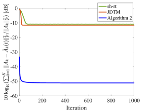
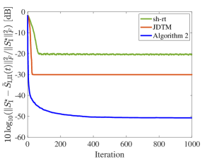
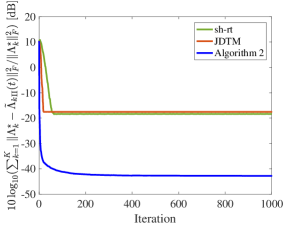
Figure 1: Transition of approximation errors in the case of SNR $50$ dB and $\kappa=50$.

Table 2: Computation time, number of iterations, until ${\left\lVert S^{\star}_{\mathrm{I}}-{\tilde{S}}_{\mathrm{I,II}}(t)\right\rVert}_{F}^{2}/{\left\lVert S_{\mathrm{I}}^{\star}\right\rVert}_{F}^{2}\leq 10^{-2},10^{-3}$, or $10^{-4}$, and rate of successful trials (from left to right) in the case of SNR $50$ dB and $\kappa=50$. Note that we use ”-” if the rate of successful trials is smaller than $10\%$.

${\left\lVert S^{\star}_{\mathrm{I}}-{\tilde{S}}_{\mathrm{I,II}}(t)\right\rVert}_{F}^{2}/{\left\lVert S_{\mathrm{I}}^{\star}\right\rVert}_{F}^{2}$	$\leq 10^{-2}$			$\leq 10^{-3}$			$\leq 10^{-4}$
sh-rt [14]	$4.298$ ms	$52.69$	$75\%$	-	-	$8\%$	-	-	$2\%$
JDTM [5]	$\mathbf{1.552}$ ms	$18.85$	$100\%$	$\mathbf{1.873}$ ms	$22.99$	$72\%$	-	-	$8\%$
Algorithm 2	$4.004$ ms	$\mathbf{1.610}$	$100\%$	$5.212$ ms	$\mathbf{3.540}$	$\mathbf{100\%}$	$12.32$ ms	$\mathbf{14.79}$	$\mathbf{100\%}$

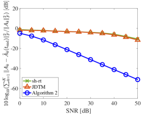
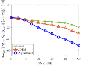
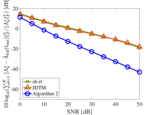
Figure 2: Comparison of ASD algorithms for $S^{\star}$ of condition number $\kappa=50$.

Table 3: Computation time, number of iterations, until ${\left\lVert S^{\star}_{\mathrm{I}}-{\tilde{S}}_{\mathrm{I,II}}(t)\right\rVert}_{F}^{2}/{\left\lVert S_{\mathrm{I}}^{\star}\right\rVert}_{F}^{2}\leq 10^{-2},10^{-3}$, or $10^{-4}$, and rate of successful trials (from left to right) in the case of SNR $50$ dB and $\kappa=5$.

${\left\lVert S^{\star}_{\mathrm{I}}-{\tilde{S}}_{\mathrm{I,II}}(t)\right\rVert}_{F}^{2}/{\left\lVert S_{\mathrm{I}}^{\star}\right\rVert}_{F}^{2}$	$\leq 10^{-2}$			$\leq 10^{-3}$			$\leq 10^{-4}$
sh-rt [14]	$2.139$ ms	$21.27$	$100\%$	$2.542$ ms	$26.83$	$100\%$	$2.777$ ms	$29.72$	$100\%$
JDTM [5]	$\mathbf{1.227}$ ms	$14.09$	$100\%$	$\mathbf{1.425}$ ms	$17.13$	$100\%$	$\mathbf{1.603}$ ms	$19.06$	$100\%$
Algorithm 2	$3.208$ ms	$\mathbf{1.000}$	$100\%$	$3.334$ ms	$\mathbf{1.000}$	$100\%$	$3.338$ ms	$\mathbf{1.000}$	$100\%$

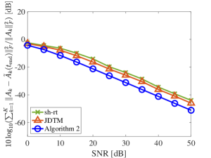
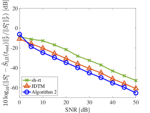
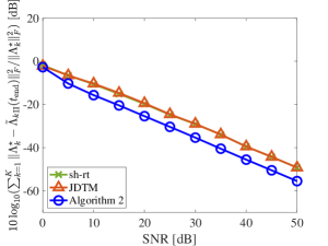
Figure 3: Comparison of ASD algorithms for $S^{\star}$ of condition number $\kappa=5$.

To see the numerical performance of Algorithm 2, in comparison to the two Jacobi-like methods (sh-rt [14] and JDTM [5]), under several conditions (e.g., noise levels, condition numbers of an ideal common diagonalizer), we conduct numerical experiments for a perturbed version ${\mathbf{A}}=(A_{1},\ldots,A_{K})\in{\bigtimes_{k=1}^{K}}{\mathbb{R}^{n\times n}}\ (n=5,K=20)$ of ${\mathbf{A}}^{\star}=(A^{\star}_{1},\ldots,A^{\star}_{K})\coloneqq(S^{\star}\Lambda_{k}^{\star}(S^{\star})^{-1})_{k=1}^{K}\in{\mathfrak{D}^{\mathrm{abl}}_{n,K}}$ with $A_{k}\coloneqq A_{k}^{\star}+\sigma N_{k}\ (k=1,\ldots,K)$, where the diagonal entries of diagonal matrices $\Lambda_{k}^{\star}\in{\mathbb{R}^{n\times n}}$ and all the entries of $N_{k}\in{\mathbb{R}^{n\times n}}$ are drawn from the standard normal distribution ${\mathcal{N}}(0,1)$ and $\sigma>0$ is used to define the Signal to Noise Ratio (SNR). To conduct numerical experiments for $S^{\star}\in{\mathbb{R}^{n\times n}}$ of various condition numbers, say $\kappa>1$, we design $S^{\star}$ by replacing singular values, of a matrix whose entries are drawn from the standard normal distribution ${\mathcal{N}}(0,1)$, with $\sigma_{i}(S^{\star})\coloneqq(\kappa-1)(n-i)/(n-1)+1(i=1,\ldots,n)$ implying thus $\sigma_{1}(S^{\star})/\sigma_{n}(S^{\star})=\kappa$. For Algorithm 2, we use, as the $t$th estimates, ${\tilde{S}}(t)\coloneqq$ DODO($P_{\Xi^{-1}({\hat{A}}(t))}({\mathbf{A}}),n$) if $P_{\Xi^{-1}({\hat{A}}(t))}({\mathbf{A}})\in{\mathfrak{D}^{\mathrm{abl}}_{n,K}}$; otherwise ${\tilde{S}}(t)\coloneqq$ PCD($P_{\Xi^{-1}({\hat{A}}(t))}({\mathbf{A}})$) (see function PCD in Algorithm 2), ${\tilde{{\mathbf{A}}}}(t)=({\tilde{A}}_{1}(t),\ldots,{\tilde{A}}_{K}(t))\coloneqq P_{\Xi^{-1}({\hat{A}}(t))}({\mathbf{A}})$ if $P_{\Xi^{-1}({\hat{A}}(t))}({\mathbf{A}})\in{\mathfrak{D}^{\mathrm{abl}}_{n,K}}$; otherwise ${\tilde{{\mathbf{A}}}}(t)\coloneqq P_{{\mathfrak{D}^{\mathrm{abl}}_{n,K}}({\tilde{S}}(t))}({\mathbf{A}})$, and ${\tilde{\Lambda}}_{k}(t)\coloneqq({\tilde{S}}(t))^{-1}{\tilde{A}}_{k}(t){\tilde{S}}(t)\ (k=1,\ldots,K;t=0,1,\ldots)$. For the Jacobi-like methods, on the other hand, we use, as the $t$th estimates, ${\tilde{S}}(t)\coloneqq\breve{S}(t)$, ${\tilde{\Lambda}}_{k}(t)\coloneqq\breve{\Lambda}_{k}(t)$, where $\breve{S}(t)$ and $\breve{\Lambda}_{k}(t)$ are respectively the $t$th updates of $\breve{S}$ and $\breve{\Lambda}$ in the Jacobi-like methods (sh-rt and JDTM; see Section 2.2 for sh-rt), and ${\tilde{A}}_{k}(t)\coloneqq{\tilde{S}}(t){\tilde{\Lambda}}_{k}(t)({\tilde{S}}(t))^{-1}\ (k=1,\ldots,K)$. The Jacobi-like methods are terminated when the number of iteration exceeds $2\times 10^{4}$ or when $\left\lvert f_{\mathbf{A}}({\tilde{S}}(t))-f_{{\mathbf{A}}}({\tilde{S}}(t-1))\right\rvert/\left\lvert f_{{\mathbf{A}}}({\tilde{S}}(t))\right\rvert\leq 10^{-6}\ (t\in{\mathbb{N}})$, where $f_{\mathbf{A}}({\tilde{S}}(t))=\sum_{k=1}^{K}{\operatorname{off}}(({\tilde{S}}(t))^{-1}A_{k}{\tilde{S}}(t))$. We choose $\varepsilon=10^{-6}$ and $t_{\mathrm{max}}=2\times 10^{4}$ in Algorithm 2. For each algorithm, we use $t_{\mathrm{end}}\in{\mathbb{N}}$ to indicate the iteration when the algorithm is terminated. We evaluate the approximation errors of ${\tilde{S}}(t)$, $({\tilde{\Lambda}}_{1}(t),\ldots,{\tilde{\Lambda}}_{K}(t))$, ${\tilde{{\mathbf{A}}}}(t)=({\tilde{A}}_{1}(t),\ldots,{\tilde{A}}_{k}(t))$ by ${\left\lVert S^{\star}_{\mathrm{I}}-{\tilde{S}}_{\mathrm{I,II}}(t)\right\rVert}^{2}_{F}/{\left\lVert S^{\star}_{\mathrm{I}}\right\rVert}^{2}_{F}$, $\sum_{k=1}^{K}{\left\lVert\Lambda^{\star}_{k}-\mbox{${\tilde{\Lambda}}_{k}$}_{\mathrm{II}}(t)\right\rVert}^{2}_{F}/{\left\lVert\Lambda^{\star}_{k}\right\rVert}^{2}_{F}$, and $\sum_{k=1}^{K}{\left\lVert A_{k}-{\tilde{A}}_{k}(t)\right\rVert}^{2}_{F}/{\left\lVert A_{k}\right\rVert}^{2}_{F}$, respectively, where (i) $S^{\star}_{\mathrm{I}}$ stands for the column-wise normalization of $S^{\star}$ and ${\tilde{S}}_{\mathrm{I,II}}(t)$ stands for the column-wise permutation applied to achieve the best approximation to $S_{I}^{\star}$ after the column-wise normalization of ${\tilde{S}}(t)$, and (ii) $\mbox{${\tilde{\Lambda}}_{k}$}_{\mathrm{II}}(t)$ stands for the diagonal matrix after applying the corresponding permutation for ${\tilde{S}}_{\mathrm{I,II}}(t)$ to diagonal entries of ${\tilde{\Lambda}}_{k}(t)$.

We conducted numerical experiments on Intel Core i7-8559U running at $2.7$ GHz with $4$ cores and $32$ GB of main memory. By using Matlab, we implemented all the ASD algorithms by ourselves. We measured the computation times of all the ASD algorithms by Matlab’s tic/toc functions. We compared the computation time and the number of iterations, of all the algorithms, until ${\left\lVert S^{\star}_{\mathrm{I}}-{\tilde{S}}_{\mathrm{I,II}}(t)\right\rVert}_{F}^{2}/{\left\lVert S^{\star}_{\mathrm{I}}\right\rVert}_{F}^{2}\leq 10^{-2},10^{-3}$, and $10^{-4}\ (t=0,1,\ldots)$ as shown in Table 2 and 3. For each ASD algorithm, the successful trial means a trial where the algorithm succeeds in achieving smaller approximation error of ${\tilde{S}}(t)$ than prescribed values $10^{-2},10^{-3}$, and $10^{-4}$ before termination of each algorithm.

Since it is reported in [5] that the Jacobi-like methods tend to suffer from the cases where the input tuple is a perturbed version of a simultaneously diagonalizable tuple with a common diagonalizer of large condition number, we first compared all the ASD algorithms for $\kappa=50$. Figure 1 depicts the transition of the mean values, of the relative squared errors of ${\tilde{{\mathbf{A}}}}(t),{\tilde{S}}(t)$ and $({\tilde{\Lambda}}_{1}(t),\ldots,{\tilde{\Lambda}}_{K}(t))$ after proper column-wise normalization/permutation for ${\tilde{S}}(t)$ and $({\tilde{\Lambda}}_{k}(t))_{k=1}^{K}$, over $100$ trials in the case of SNR $50$ dB. Figure 1 illustrates that, compared with the Jacobi-like methods, Algorithm 2 achieves estimations (i) ${\tilde{{\mathbf{A}}}}(t)\in{\mathfrak{D}^{\mathrm{abl}}_{n,K}}$, of ${\mathbf{A}}^{\star}$, closer to ${\mathbf{A}}$, (ii) ${\tilde{S}}_{\mathrm{I,II}}(t)$, of $S_{\mathrm{I}}^{\star}$, closer to $S_{\mathrm{I}}^{\star}$, and (iii) $(\mbox{${\tilde{\Lambda}}_{k}$}_{\mathrm{II}}(t))_{k=1}^{K}$, of $(\Lambda^{\star}_{k})_{k=1}^{K}$, closer to $(\Lambda^{\star}_{k})_{k=1}^{K}$ with smaller number of iterations. Table 2 depicts the mean values of (i) the computation times and (ii) the numbers of iterations taken until ${\left\lVert S^{\star}_{\mathrm{I}}-{\tilde{S}}_{\mathrm{I,II}}(t)\right\rVert}_{F}^{2}/{\left\lVert S_{\mathrm{I}}^{\star}\right\rVert}_{F}^{2}\leq 10^{-2},10^{-3}$, or $10^{-4}$ over successful trials in $100$ trials and (iii) the rates of successful trials over $100$ trials. This result shows that Algorithm 2 takes around $3$ times longer computation time than JDTM but its ${\tilde{S}}(t_{\mathrm{end}})$ achieves the prescribed conditions even for the trials where the Jacobi-like methods fail to achieve the prescribed conditions. Figure 2 depicts the mean values, of the relative squared errors of ${\tilde{{\mathbf{A}}}}(t_{\mathrm{end}}),{\tilde{S}}(t_{\mathrm{end}})$, and $({\tilde{\Lambda}}_{k}(t_{\mathrm{end}}))_{k=1}^{K}$ after proper column-wise normalization/permutation for ${\tilde{S}}(t)$ and $({\tilde{\Lambda}}_{k}(t))_{k=1}^{K}$, over $100$ trials in the cases of SNR from $0$ dB to $50$ dB. Figure 2 illustrates Algorithm 2 outperforms the Jacobi-like methods in the sense of achieving approximation errors at $t_{\mathrm{end}}$ especially when SNR is higher than $10$ dB.

We also compared all the algorithms in the case of $\kappa=5$. All the values in Table 3 and Figure 3 are calculated by the same way as done for $\kappa=50$. Figure 3 and Table 3 show that Algorithm 2 takes around $3$ times longer computation time than JDTM but can outperform the Jacobi-like methods in the sense of achieving approximation errors at $t_{\mathrm{end}}$ in SNR from $5$ dB to $50$ dB. From these experiments, we see that Algorithm 2 is robust against wider range of condition numbers of $S^{\star}$ than the Jacobi-like methods.

5 Concluding Remarks

In this paper, for the approximate simultaneous diagonalization of ${\mathbf{A}}\in{\bigtimes_{k=1}^{K}}{\mathbb{C}^{n\times n}}$, we newly presented the Approximate-Then-Diagonalize-Simultaneously (ATDS) algorithm by solving a certain Structured Low-Rank Approximation (SLRA). For ${\mathbf{A}}\in{\mathfrak{D}^{\mathrm{abl}}_{n,K}}$, the proposed ATDS algorithm has a guarantee to find its common exact diagonalizer unlike the Jacobi-like methods. Numerical experiments show that, at the expense of reasonable computational time, the proposed ATDS algorithm achieves better approximations to the desired information in Problem 2 than the Jacobi-like methods for almost all SNR as well as both for small and large condition numbers of $S^{\star}$.

The reduction of the computational cost for SVD of ${\hat{A}}(t)\in{\mathbb{C}}^{Kn^{2}\times n^{2}}\ (t=0,1,\ldots)$ in Algorithm 2 is under study. We are also studying applications of the proposed ATDS algorithm to certain signal processing problems. These will be reported elsewhere.

Appendix A Nonconvexity of ${\mathfrak{D}}^{\mathrm{abl}}_{2,2}$

The following simple example shows the nonconvexity of ${\mathfrak{D}}^{\mathrm{abl}}_{2,2}\subsetneq{\mathbb{C}}^{2\times 2}\times{\mathbb{C}}^{2\times 2}$. Let $A_{1}\coloneqq\big{[}\begin{smallmatrix}1&1\\ -1&1\end{smallmatrix}\big{]},A_{2}\coloneqq 2A_{1},B_{1}\coloneqq\big{[}\begin{smallmatrix}1&1\\ 1&1\end{smallmatrix}\big{]}$, and $B_{2}\coloneqq 2B_{1}$. Since $A_{1},A_{2},B_{1}$ and $B_{2}$ are normal, these are respectively diagonalizable [20, Theorem 2.5.3]. Moreover, by $A_{1}A_{2}=A_{2}A_{1}$ and $B_{1}B_{2}=B_{2}B_{1}$, we see ${\mathbf{A}}\coloneqq(A_{1},A_{2}),{\mathbf{B}}\coloneqq(B_{1},B_{2})\in{\mathfrak{D}}^{\mathrm{abl}}_{2,2}$ (see Fact 2 in Section 2.1). Below, we will show that ${\mathbf{A}}/2+{\mathbf{B}}/2\not\in{\mathfrak{D}}^{\mathrm{abl}}_{2,2}$. Since every eigenvector of $(A_{1}+B_{1})/2=\big{[}\begin{smallmatrix}1&1\\ 0&1\end{smallmatrix}\big{]}$ is given by ${\mathbf{v}}=\big{[}\begin{smallmatrix}v\\ 0\end{smallmatrix}\big{]}\ (v\in{\mathbb{C}}\setminus\{0\})$, the eigenspace of $\big{[}\begin{smallmatrix}1&1\\ 0&1\end{smallmatrix}\big{]}$ has dimension $1$, which implies $(A_{1}+B_{1})/2$ is not diagonalizable and hence ${\mathbf{A}}/2+{\mathbf{B}}/2\not\in{\mathfrak{D}}^{\mathrm{abl}}_{2,2}$.

Appendix B Useful Facts on Commutativity and Diagonalizability

Fact 3 (On commutativity).

1. For a given $X\in{\mathbb{C}^{n\times n}}$, the set of all matrices which commute with $X$ is a subspace of ${\mathbb{C}^{n\times n}}$ with dimension at least $n$; the dimension is equal to $n$ if and only if each eigenvalue of $X$ has geometric multiplicity $1$, i.e., $X$ is nonderogatory [30, Corollary 4.4.15].

2. For a given $X\in{\mathbb{C}^{n\times n}}$, $X$ is nonderogatory if and only if every matrix $Y\in{\mathbb{C}^{n\times n}}$ which commutes with $X$ can be expressed as $Y=c_{0}I+c_{1}X+c_{2}X^{2}+\cdots+c_{n-1}X^{n-1}$ for some $c_{0},c_{1},\ldots,c_{n-1}\in{\mathbb{C}}$, i.e., $Y$ is a polynomial in $X$ [30, Corollary 4.4.18].

3. Let $\lambda_{1},\ldots,\lambda_{d}\in{\mathbb{C}}$ be distinct and let $\Lambda=\lambda_{1}I_{n_{1}}\oplus\cdots\oplus\lambda_{d}I_{n_{d}}\in{\mathbb{C}^{n\times n}}$. Then, for $X=[X_{i,j}]_{i,j=1}^{d}\in{\mathbb{C}^{n\times n}}\ (X_{i,j}\in{\mathbb{C}}^{n_{i}\times n_{j}})$, $\Lambda X=X\Lambda\Leftrightarrow X=X_{1,1}\oplus\cdots\oplus X_{d,d}$ (Note: (c) is verified by $\Lambda X=X\Lambda\Leftrightarrow(\forall i,j\in\{1,\ldots,d\})\lambda_{i}X_{i,j}=\lambda_{j}X_{i,j}$, and $(\forall i\neq j)\lambda_{i}X_{i,j}=\lambda_{j}X_{i,j}\Rightarrow(\forall i\neq j)X_{i,j}=O$).

Fact 4 (On diagonalizability of block diagonal matrix [20, Lemma 1.3.10]).

Suppose $X=\check{X}_{1}\oplus\cdots\oplus\check{X}_{l}\in{\mathbb{C}^{n\times n}}$ for some $X_{p}\in{\mathbb{C}}^{n_{p}\times n_{p}}\ (n_{1}+\cdots+n_{l}=n)$. Then $X\in{\mathsf{D}^{\mathrm{abl}}_{n}}\Leftrightarrow(\forall p\in\{1,\ldots,l\})\check{X}_{p}\in{\mathsf{D}}^{\mathrm{abl}}_{n_{p}}$.

Appendix C Structured Low-Rank Approximation

Structured Low-Rank Approximation (SLRA) [17] is a problem, for a given matrix $A\in{\mathbb{C}^{m\times n}}$, a given integer $r\in(0,\min\{m,n\})$, and a given affine subspace $\Omega\subset{\mathbb{C}^{m\times n}}$, to find a minimizer, in all matrices of rank at most $r$, of ${\left\lVert A-X\right\rVert}^{2}_{F}$. SLRA has many applications in signal processing (see e.g., [17] and references therein).

For SLRA, Cadzow’s algorithm [18] also known as alternating projection algorithm has been used extensively while some methods to find its local minimizer [31, 32] or its global one [33] also have been proposed. It is reported that, in practice, Cadzow’s algorithm finds a structured low-rank matrix close to a given one [18].

Appendix D Proof of Theorem 1

1. This follows from the expression of the condition $X_{k}X_{l}-X_{l}X_{k}=O\ (k,l=1,\ldots,K)$ in vector form.

2. (Proof of ”$\Rightarrow$”) Let $X_{k}=S\Lambda_{k}S^{-1}$ be such that $\Lambda_{k}\in{\mathbb{C}^{n\times n}}\ (k=1,\ldots,K)$ are diagonal. By using identities: $(A\otimes B)(C\otimes D)=AC\otimes BD\ (A,B,C,D\in{\mathbb{C}^{n\times n}})$ [30, Lemma 4.2.10] and $(A\otimes B)^{-1}=A^{-1}\otimes B^{-1}\ (A,B\in{\mathbb{C}^{n\times n}})$ [30, Corollary 4.2.11], we get $I_{n}\otimes X_{k}-X_{k}^{\top}\otimes I_{n}=(S^{-\top}\otimes S)(I_{n}\otimes\Lambda_{k}-\Lambda_{k}\otimes I_{n})(S^{-\top}\otimes S)^{-1}$. Since $(I_{n}\otimes\Lambda_{k}-\Lambda_{k}\otimes I_{n})$ is diagonal and the $((j-1)n+j)$th diagonal entry is $0$ for every $j=1,\ldots,n$, we see $(\forall k\in\{1,\ldots,K\})\ {\operatorname{nullspace}}(I_{n}\otimes X_{k}-X_{k}^{\top}\otimes I_{n})\supset{\operatorname{range}}(S^{-\top}\odot S)\Leftrightarrow{\operatorname{nullspace}}(\Xi({\mathbf{X}}))\supset{\operatorname{range}}(S^{-\top}\odot S)$.

   (Proof of ”$\Leftarrow$”)  Note first that any ${\mathbf{y}}\in{\operatorname{range}}(S^{-\top}\odot S)$ can be expressed with $\boldsymbol{\lambda}\coloneqq[\lambda_{i}]\in{\mathbb{C}^{n}}$ as ${\mathbf{y}}=(S^{-\top}\odot S)\boldsymbol{\lambda}$ and that $Y\coloneqq{\operatorname{vec}}^{-1}({\mathbf{y}})=S{\operatorname{diag}}(\lambda_{1},\ldots,\lambda_{n})S^{-1}$, where we used the well-known identity ${\operatorname{vec}}(A{\operatorname{diag}}({\mathbf{d}})C)=(C^{\top}\odot A){\mathbf{d}}\ (A,C\in{\mathbb{C}^{n\times n}};{\mathbf{d}}\in{\mathbb{C}^{n}})$ (see, e.g., [28, Property 1]). By ${\mathbf{y}}\in{\operatorname{nullspace}}(\Xi({\mathbf{X}}))$ and (a), we see $X_{k}Y=YX_{k}\ (k=1,\ldots,K)$. Choose specially $\boldsymbol{\lambda}$ such that all entries $\lambda_{i}\ (i=1,\ldots,n)$ are distinct in order to ensure $Y$ is nonderogatory. In this case, Fact 3(b) ensures that $X_{k}\ (k=1,\ldots,K)$ are polynomials in $Y$, say $X_{k}=\mathcal{P}_{k}(Y)$, and therefore, $X_{k}=S{\operatorname{diag}}(\mathcal{P}_{k}(\lambda_{1}),\ldots,\mathcal{P}_{k}(\lambda_{n}))S^{-1}$, which implies ${\mathbf{X}}\in{\mathfrak{D}^{\mathrm{abl}}_{n,K}}$.

3. Let $X_{k}=S\Lambda_{k}S^{-1}$ be such that $\Lambda_{k}\in{\mathbb{C}^{n\times n}}\ (k=1,\ldots,K)$ are diagonal. Since ${\operatorname{dim}}({\operatorname{range}}(S^{-\top}\odot S))=n$, we see from (b) that ${\operatorname{dim}}({\operatorname{nullspace}}(\Xi({\mathbf{X}})))\geq n\Leftrightarrow{\operatorname{rank}}(\Xi({\mathbf{X}}))\leq n^{2}-n$. Moreover, since $\Xi({\mathbf{X}})=(I_{K}\otimes(S^{-\top}\otimes S))\Xi(\Lambda_{1},\Lambda_{2},\ldots,\Lambda_{K})(S^{-\top}\otimes S)^{-1}$, we see ${\operatorname{rank}}(\Xi({\mathbf{X}}))={\operatorname{rank}}(\Xi(\Lambda_{1},\ldots,\Lambda_{K}))$. Fact 1 ensures the simultaneous diagonalization of ${\mathbf{X}}$ is essentially unique if and only if $\Xi(\boldsymbol{\Lambda})$ has just $n$ zero vectors as the column vectors, i.e., ${\operatorname{rank}}(\Xi(\Lambda_{1},\ldots,\Lambda_{K}))=n^{2}-n$.

4. (Proof of ”$\Rightarrow$”) It follows from Fact 1 and (c).

   (Proof of ”$\Leftarrow$”) Suppose that $X_{1}$ has $n$ distinct eigenvalues. Therefore, there exist $S\in{\mathbb{C}^{n\times n}}$ and a diagonal matrix $\Lambda_{1}\in{\mathbb{C}^{n\times n}}$ such that $X_{1}=S\Lambda_{1}S^{-1}$. By Fact 3(a), ${\operatorname{dim}}({\operatorname{nullspace}}(I_{n}\otimes X_{1}-X_{1}^{\top}\otimes I_{n}))=n$ and hence ${\operatorname{nullspace}}(\Xi({\mathbf{X}}))={\operatorname{nullspace}}(I_{n}\otimes X_{1}-X_{1}^{\top}\otimes I_{n})$. For any $k=2,\ldots,K$, moreover, ${\operatorname{nullspace}}(I_{n}\otimes X_{k}-X_{k}^{\top}\otimes I_{n})\supseteq{\operatorname{nullspace}}(\Xi({\mathbf{X}}))={\operatorname{nullspace}}(I_{n}\otimes X_{1}-X_{1}^{\top}\otimes I_{n})\ni{\operatorname{vec}}(X_{1})$, which ensures the commutativity of $X_{1}$ and $X_{k}$. By using Fact 3(b), we see that each $X_{k}$ is a certain polynomial in $X_{1}$. Therefore, $S^{-1}X_{k}S\ (k=2,\ldots,K)$ are diagonal.

5. From (d), it is sufficient to show ${\operatorname{rank}}(\Xi({\mathbf{Y}}))=n^{2}-n$. Since $Y_{l}$ has $n$ distinct eigenvalues, Fact 3(a) and $\Xi({\mathbf{Y}})\in{\mathfrak{L}}_{n^{2}-n}$ ensure $n^{2}-n={\operatorname{rank}}(I_{n}\otimes Y_{l}-Y_{l}^{\top}\otimes I_{n})\leq{\operatorname{rank}}(\Xi({\mathbf{Y}}))\leq n^{2}-n$. ∎

Appendix E Proof of Proposition 1

1. It is clear that ${\mathbf{X}}\in({\operatorname{span}}\{I_{n}\})^{K}\Leftrightarrow\Xi({\mathbf{X}})=O$.
   (proof of ”$\supset$”) Since, for any ${\mathbf{X}}\in{\mathbf{X}}^{\diamond}+({\operatorname{span}}\{I_{n}\})^{K}$, $\Xi({\mathbf{X}})=\Xi({\mathbf{X}}^{\diamond})={\hat{X}}$ holds, we see ${\mathbf{X}}\in\Xi^{-1}({\hat{X}})$.
   (proof of ”$\subset$”) For any ${\mathbf{X}}\in\Xi^{-1}({\hat{X}})$, we have $\Xi({\mathbf{X}}-{\mathbf{X}}^{\diamond})=O\Leftrightarrow{\mathbf{X}}-{\mathbf{X}}^{\diamond}\in({\operatorname{span}}\{I_{n}\})^{K}$, where ${\mathbf{X}}^{\diamond}\in\Xi^{-1}({\hat{X}})$. Therefore ${\mathbf{X}}\in{\mathbf{X}}^{\diamond}+({\operatorname{span}}\{I_{n}\})^{K}$.

2. This follows from (a) and equalities

   $$\min_{(Y_{1},\ldots,Y_{K})\in\Xi^{-1}({\hat{X}})}\sum_{k=1}^{K}{\left\lVert X_{k}-Y_{k}\right\rVert}_{F}^{2}$$

   $$=\min_{\begin{subarray}{c}\alpha_{1},\ldots,\alpha_{k}\in\mathbb{C}\end{subarray}}\sum_{k=1}^{K}{\left\lVert X_{k}-X^{\diamond}_{k}-\alpha_{k}I_{n}\right\rVert}^{2}_{F}$$

   $$=\sum_{k=1}^{K}{\left\lVert X_{k}-X^{\diamond}_{k}-P_{{\operatorname{span}}\{I_{n}\}}(X_{k}-X^{\diamond}_{k})\right\rVert}^{2}_{F}.$$

3. For $X=[x_{i,j}]\in{\mathbb{C}^{n\times n}}$ and $Y=[y_{i,j}]\in{\mathbb{C}^{n\times n}}$,

   $${\left\lVert I_{n}\otimes X-X^{\top}\otimes I_{n}-I_{n}\otimes Y-Y^{\top}\otimes I_{n}\right\rVert}^{2}_{F}$$

   $$=\sum_{i=1}^{n}{\left\lVert X-x_{i,i}I_{n}-Y+y_{i,i}I_{n}\right\rVert}^{2}_{F}$$

   $$\quad+n\sum_{\begin{subarray}{c}p,q=1,p\neq q\end{subarray}}^{n}\left\lvert x_{p,q}-y_{p,q}\right\rvert^{2}$$

   $$=n{\left\lVert X-Y\right\rVert}^{2}_{F}+n\sum_{i=1}^{n}\left\lvert x_{i,i}-y_{i,i}\right\rvert^{2}$$

   $$\quad-2\left\lvert{\operatorname{tr}}(X-Y)\right\rvert^{2}+n\sum_{\begin{subarray}{c}p,q=1,p\neq q\end{subarray}}^{n}\left\lvert x_{p,q}-y_{p,q}\right\rvert^{2}$$

   $$=2n{\left\lVert X-Y\right\rVert}^{2}_{F}-2\left\lvert{\operatorname{tr}}(X-Y)\right\rvert^{2}.$$

   Hence ${\left\lVert\Xi({\mathbf{X}})-{\hat{X}}\right\rVert}^{2}_{F}={\left\lVert\Xi({\mathbf{X}})-\Xi(Z_{1},\ldots,Z_{K})\right\rVert}_{F}^{2}=\sum_{k=1}^{K}2n{\left\lVert X_{k}-Z_{k}\right\rVert}^{2}_{F}-2\left\lvert{\operatorname{tr}}(X_{k}-Z_{k})\right\rvert^{2}$. Since (b) ensures ${\operatorname{tr}}(X_{k}-Z_{k})=0\ (k=1,\ldots,K)$, we get $\sum_{k=1}^{K}{\left\lVert X_{k}-Z_{k}\right\rVert}^{2}_{F}={\left\lVert\Xi({\mathbf{X}})-{\hat{X}}\right\rVert}^{2}_{F}/2n$. ∎

Appendix F Proof of Proposition 2

This follows from ${\left\lVert\Xi({\tilde{{\mathbf{A}}}}(t))-P_{{\mathfrak{L}}_{n^{2}-n}}(\Xi({\tilde{{\mathbf{A}}}}(t)))\right\rVert}_{F}\\ \geq{\left\lVert\Xi({\tilde{{\mathbf{A}}}}(t+1))-P_{{\mathfrak{L}}_{n^{2}-n}}(\Xi({\tilde{{\mathbf{A}}}}(t)))\right\rVert}_{F}\\ \geq{\left\lVert\Xi({\tilde{{\mathbf{A}}}}(t+1))-P_{{\mathfrak{L}}_{n^{2}-n}}(\Xi({\tilde{{\mathbf{A}}}}(t+1)))\right\rVert}_{F}$. ∎

[./Images/akema.eps]Riku Akema received the B.E. degree in computer science and M.E. degree in information and communications engineering from the Tokyo Institute of Technology in 2016 and 2018, respectively. Currently, he is a Ph.D. student in the Department of Information and Communications Engineering, Tokyo Institute of Technology. His current research interests are in signal processing and multi-way data analytics. [./Images/Masao_Yamagishi_Gray.eps]Masao Yamagishi received the B.E. degree in computer science and the M.E. and Ph.D. degrees in communications and integrated systems from the Tokyo Institute of Technology, Tokyo, Japan, in 2007, 2008, and 2012, respectively. Currently, he is an assistant professor with the Department of Information and Communications Engineering, Tokyo Institute of Technology. [./Images/IsaoYamada.eps]Isao Yamada received the B.E. degree in computer science from the University of Tsukuba in 1985 and the M.E. and the Ph.D. degrees in electrical and electronic engineering from the Tokyo Institute of Technology, in 1987 and 1990. Currently, he is a professor with the Department of Information and Communications Engineering, Tokyo Institute of Technology. He has been the IEICE Fellow and IEEE Fellow since 2015.

References

- [1] I.T. Jolliffe, Principal Component Analysis, 2nd ed., Springer-Verlag, 2002.
- [2] C.M. Bishop, Pattern Recognition and Machine Learning, Springer, 2006.
- [3] L. De Lathauwer, B. De Moor, and J. Vandewalle, “Computation of the canonical decomposition by means of a simultaneous generalized Schur decomposition,” SIAM J. Matrix Anal. Appl., vol.26, no.2, pp.295–327, 2004.
- [4] F. Roemer and M. Haardt, “A semi-algebraic framework for approximate CP decompositions via simultaneous matrix diagonalizations (SECSI),” Signal Processing, vol.93, no.9, pp.2722–2738, 2013.
- [5] X. Luciani and L. Albera, “Canonical Polyadic Decomposition based on joint eigenvalue decomposition,” Chemom. Intell. Lab. Syst., vol.132, pp.152–167, 2014.
- [6] R. André, X. Luciani, and E. Moreau, “Joint EigenValue Decomposition Algorithms Based on First-Order Taylor Expansion,” IEEE Trans. Signal Process., vol.68, pp.1716–1727, 2020.
- [7] J.F. Cardoso and A. Souloumiac, “Blind beamforming for non-Gaussian signals,” IEE Proc. F Radar Signal Process., vol.140, no.6, pp.362–370, 1993.
- [8] L. Albera, A. Ferréol, P. Chevalier, and P. Comon, “ICAR: A Tool for Blind Source Separation Using Fourth-Order Statistics Only,” IEEE Trans. Signal Process., vol.53, no.10, pp.3633–3643, 2005.
- [9] L. De Lathauwer and J. Castaing, “Blind identification of underdetermined mixtures by simultaneous matrix diagonalization,” IEEE Trans. Signal Process., vol.56, no.3, pp.1096–1105, 2008.
- [10] X. Luciani and L. Albera, “Joint Eigenvalue Decomposition of Non-Defective Matrices Based on the LU Factorization With Application to ICA,” IEEE Trans. Signal Process., vol.63, no.17, pp.4594–4608, 2015.
- [11] A.J. van der Veen, P.B. Ober, and E.F. Deprettere, “Azimuth and Elevation Computation in High Resolution DOA Estimation,” IEEE Trans. Signal Process., vol.40, no.7, pp.1828–1832, 1992.
- [12] A.N. Lemma, A.J. van der Veen, and E.F. Deprettere, “Analysis of Joint Angle-Frequency Estimation Using ESPRIT,” IEEE Trans. Signal Process., vol.51, no.5, pp.1264–1283, 2003.
- [13] M. Haardt, R.S. Thoma, and A. Richter, “Multidimensional high-resolution parameter estimation with applications to channel sounding,,” in High-Resolution Robust Signal Process., pp.253–338, Marcel Dekker, 2004.
- [14] T. Fu and X. Gao, “Simultaneous Diagonalization with Similarity Transformation for Non-Defective Matrices,” IEEE Int. Conf. Acoust. Speech, Signal Process., pp.1137–1140, 2006.
- [15] R. Iferroudjene, K. Abed-meraim, and A. Belouchrani, “A new Jacobi-like method for joint diagonalization of arbitrary non-defective matrices,” Appl. Math. Comput., vol.211, no.2, pp.363–373, 2009.
- [16] A. Bunse-Gerstner, R. Byers, and V. Mehrmann, “Numerical Methods for Simultaneous Diagonalization,” SIAM J. Matrix Anal. Appl., vol.14, no.4, pp.927–949, 1993.
- [17] I. Markovsky, “Structured low-rank approximation and its applications,” Automatica, vol.44, no.4, pp.891–909, 2008.
- [18] J.A. Cadzow, “Signal Enhancement―A Composite Property Mapping Algorithm,” IEEE Trans. Acoust. Speech Signal Process., vol.36, pp.49–62, 1988.
- [19] R. Akema, M. Yamagishi, and I. Yamada, “An Alternating Projection Algorithm for Approximate Simultaneous Diagonalization,” IEEE Int. Conf. Acoust. Speech, Signal Process., pp.4973–4977, 2019.
- [20] R.A. Horn and C.R. Johnson, Matrix Analysis, 2nd ed., Cambridge University Press, 2013.
- [21] C.G.J. Jacobi, “Über ein leichtes Verfahren die in der Theorie der Säcularstörungen vorkommenden Gleichungen numerisch aufzulösen,” J. für die reine und Angew. Math., no.30, pp.51–94, 1846.
- [22] G.H. Golub and C.F. Van Loan, Matrix Computations, 3rd ed., The Johns Hopkins University Press, 1996.
- [23] A. Ben-Israel and T.N.E. Greville, Generalized Inverses: Theory and Applications, 2nd ed., Springer-Verlag, 2003.
- [24] J. Dongarra, M. Gates, A. Haidar, J. Kurzak, P. Luszczek, S. Tomov, and I. Yamazaki, “The singular value decomposition: Anatomy of optimizing an algorithm for extreme scale,” SIAM Rev., vol.60, no.4, pp.808–865, 2018.
- [25] A.S. Lewis, D.R. Luke, and J. Malick, “Local Linear Convergence for Alternating and Averaged Nonconvex Projections,” Found. Comput. Math., vol.9, no.4, pp.485–513, 2009.
- [26] D. Noll and A. Rondepierre, “On Local Convergence of the Method of Alternating Projections,” Found. Comput. Math., vol.16, no.2, pp.425–455, 2016.
- [27] H.H. Bauschke, P.L. Combettes, and D.R. Luke, “Phase retrieval, error reduction algorithm, and Fienup variants: a view from convex optimization,” J. Opt. Soc. Am. A, vol.19, no.7, pp.1334–1345, 2002.
- [28] W.K. Ma, T.H. Hsieh, and C.Y. Chi, “DOA estimation of quasi-stationary signals with less sensors than sources and unknown spatial noise covariance: A Khatri-Rao subspace approach,” IEEE Trans. Signal Process., vol.58, no.4, pp.2168–2180, 2010.
- [29] R. Akema, M. Yamagishi, and I. Yamada, “Exploiting Commutativity Condition for CP Decomposition via Approximate Simultaneous Diagonalization,” IEEE Int. Conf. Acoust. Speech, Signal Process., pp.3287–3291, 2020.
- [30] R.A. Horn and C.R. Johnson, Topics in Matrix Analysis, Cambridge University Press, 1991.
- [31] I. Markovsky, S. Van Huffel, and R. Pintelon, “Block-Toeplitz/Hankel Structured Total Least Squares,” SIAM J. Matrix Anal. Appl., vol.26, no.4, pp.1083–1099, 2005.
- [32] É. Schost and P.J. Spaenlehauer, “A Quadratically Convergent Algorithm for Structured Low-Rank Approximation,” Found. Comput. Math., vol.16, no.2, pp.457–492, 2016.
- [33] G. Ottaviani, P.J. Spaenlehauer, and B. Sturmfels, “Exact Solutions in Structured Low-Rank Approximation,” SIAM J. Matrix Anal. Appl., vol.35, no.4, pp.1521–1542, 2014.