2-Cluster Fixed-Point Analysis of Mean-Coupled Stuart-Landau Oscillators in the Center Manifold

Abstract

We reduce the dynamics of an ensemble of mean-coupled Stuart-Landau oscillators close to the synchronized solution. In particular, we map the system onto the center manifold of the Benjamin-Feir instability, the bifurcation destabilizing the synchronized oscillation. Using symmetry arguments, we describe the structure of the dynamics on this center manifold up to cubic order, and derive expressions for its parameters. This allows us to investigate phenomena described by the Stuart-Landau ensemble, such as clustering and cluster singularities, in the lower-dimensional center manifold, providing further insights into the symmetry-broken dynamics of coupled oscillators. We show that cluster singularities in the Stuart-Landau ensemble correspond to vanishing quadratic terms in the center manifold dynamics. In addition, they act as organizing centers for the saddle-node bifurcations creating unbalanced cluster states as well for the transverse bifurcations altering the cluster stability. Furthermore, we show that bistability of different solutions with the same cluster-size distribution can only occur when either cluster contains at least $1/3$ of the oscillators, independent of the system parameters.

Keywords Globally coupled oscillators  $\cdot$ Center manifold reduction  $\cdot$ $\mathbf{S}_{N}$-equivariant systems

1 Introduction

Long-range interactions play a crucial role in various dynamical phenomena observed in nature. In a swarm of flashing fireflies, they may act as a synchronizing force, causing the swarm to flash in unison. Analogously, in an audience clapping, the acoustic sound of the clapping can be recognized by each individual, leading to clapping in unison. In these cases, long-range interactions lead to the synchronization of individual units [1].

On the other hand, long-range interactions may also lead to a split up of the individuals into two or more groups, also called dynamical clustering. In electrochemistry, a stirred electrolyte or a common resistance may induce long-range coupling, leading to spatial clustering on the electrode [2, 3, 4, 5, 6, 7, 8]. In biology, this may explain the formation of different genotypes in an otherwise homogeneous environment [9, 10].

The individual units which experience this long-range or global coupling may be oscillatory, as in the case of flashing fireflies or in a clapping audience, or, as in the case of sympatric speciation, stationary genotypes. Here, we focus on the former case of oscillatory units with long-range interactions.

Clustering in oscillatory systems with long-range interactions has been subject to theoretical investigation for many years  [11, 12, 13, 14, 15]. See also Ref. [16] for a recent review on globally coupled oscillators. In particular when the long-range interactions are weak compared to the intrinsic dynamics of the oscillator, it suffices to describe the phase evolution of each unit, and the analysis greatly simplifies [17, 18, 19]. If, however, the influence of the coupling is strong, as in the case considered here, such a reduction is no longer feasible and the amplitude dynamics must be considered. Our work aims to add to the theoretical understanding of clustering in this case of strong coupling.

From the view-point of symmetry, if the coupling between $N$ identical oscillators is global (i.e. all-to-all), then the governing equations are equivariant under the symmetric group $\mathbf{S}_{N}$. This means that the evolution equations $f$ commute with elements $\sigma$ from the symmetry group,

$$f(\sigma x)=\sigma f(x)\hskip 14.22636pt\forall\sigma\in\mathbf{S}_{N}.$$ (1)

In addition, this implies that the system has a trivial solution which is invariant under $\mathbf{S}_{N}$, that is, in which all oscillators are synchronized. Cluster states composed of two clusters, also called 2-cluster states, can then be viewed as states with the reduced symmetry $\mathbf{S}_{N_{1}}\times\mathbf{S}_{N_{2}}$, with $N_{1}$ and $N_{2}$ being the number of oscillators in each cluster. Using the equivariant branching lemma, it can then be shown that these 2-cluster states bifurcate off the trivial solution [9, 20]. The bifurcation at which the synchronized motion becomes unstable and the 2-cluster branches (also called primary branches) emerge is commonly referred to as the Benjamin-Feir instability [21, 22].

The intrinsic dimensionality of each oscillatory unit may range from $d=2$ for FitzHugh-Nagumo [23] and Van der Pol oscillators [24], via $d=3$ for the Oregonator [25] to $d=4$ for the original Hodgkin-Huxley model [26], and even higher for more detailed physical models [27]. A system composed of $N$ of these oscillators thus lives in a $d\cdot N$-dimensional phase space, making its full investigation unfeasible even for small $d$ and $N$. One can, however, circumvent this problem of increasingly large dimensions by restricting the dynamics to the center manifold of certain bifurcations. In particular, it is known that the center space of the Benjamin-Feir instability is $N-1$ dimensional [20, 28], and thus a reduction to the center manifold at this bifurcation allows for reducing the dimension of the problem to $N-1$ and thus by a factor of $\approx d$. As we show below, such a reduction lets us reveal invariant sets and bifurcation curves analytically – a difficult task in the original $d\cdot N$-dimensional space.

In this work, we focus on a particular example of a globally coupled system, in which the network is composed of oscillating units called Stuart-Landau oscillators, each represented by a complex variable $W_{k}\in\mathbb{C}$. As opposed to phase oscillators, each Stuart-Landau oscillator has two degrees of freedom, i. e. an amplitude and a phase. With a linear global coupling, the dynamics are then given by

$$\dot{W}_{k}=W_{k}-\left(1+i\gamma\right)\left|W_{k}\right|^{2}W_{k}+\left(\beta_{\textrm{r}}+i\beta_{\textrm{i}}\right)\left(\langle\mathbf{W}\rangle-W_{k}\right)$$ (2)

with the complex coupling constant $\beta_{\textrm{r}}+i\beta_{\textrm{i}}$ and the real parameter $\gamma$, also called the shear [29]. $\langle\cdot\rangle$ indicates the ensemble mean and $\dot{W}=dW/dt$. Bold face $\mathbf{W}$ indicates a vector containing the ensemble values $\left[W_{1},W_{2},\dots,W_{N}\right]$. For $\beta_{\textrm{r}}+i\beta_{\textrm{i}}=0$ the ensemble is decoupled, and each Stuart-Landau oscillator oscillates with unit amplitude and angular velocity $-\gamma$. For $\beta_{\textrm{r}}+i\beta_{\textrm{i}}\neq 0$, however, a plethora of different dynamical states can be observed. These states include fully synchronized oscillations, in which all oscillators maintain an amplitude equal to one and have a mutual phase difference of zero [30], cluster states, in which the ensemble splits up into two or more sets of synchrony [31, 32, 14], and a variety of quasi-periodic and chaotic dynamics [33, 12].

2-cluster states can be born and destroyed at saddle-node bifurcations if the number of oscillators in each cluster is different, that is, when they are unbalanced  [13]. Balanced solutions with $N_{1}=N_{2}$ emerge from the synchronized solution at the Benjamin-Feir instability. For $N=16$ oscillators and $\gamma=2$, the saddle-node bifurcations for different unbalanced cluster distributions $N_{1}\neq N_{2}$ and the Benjamin-Feir instability are depicted in Fig. 1, as a function of the coupling parameters $\beta_{\textrm{r}}$ and $\beta_{\textrm{i}}$. Here, all the 2-cluster solutions exist locally in parameter space below their respective saddle-node bifurcation curve, that is for smaller $\beta_{\textrm{r}}$ values. Up to the Benjamin-Feir instability they coexist with the stable synchronized solution. Descending from large $\beta_{\textrm{r}}$ values, notice that the most-unbalanced cluster state with $N_{1}:N_{2}=1:15$ is created first. The more balanced cluster states are born subsequently, depending on their distribution, until eventually the balanced cluster state $N_{1}:N_{2}=8:8$ is born at the Benjamin-Feir instability. At $\beta_{\textrm{r}}=-(1-\sqrt{3}\gamma)/2$, $\beta_{\textrm{i}}=(-\gamma-\sqrt{3})/2$, there exists a codimension-two point where the saddle-node bifurcations of all cluster distributions coincide. This point is called a cluster singularity [32]. Note that the qualitative picture in Fig. 1 does not change when increasing the total number of oscillators $N$. For large numbers $N\rightarrow\infty$ we expect a bow-tie-shaped band of saddle-node bifurcation curves, ranging from the saddle-node bifurcation of the most unbalanced cluster state to the Benjamin-Feir instability. As argued in Ref. [32], the cluster singularity can thus be viewed as an organizing center. By projecting the dynamics close to the Benjamin-Feir instability onto its center manifold, we aim to obtain further insights into the properties of this organizing center, and to elucidate the clustering behavior near it.

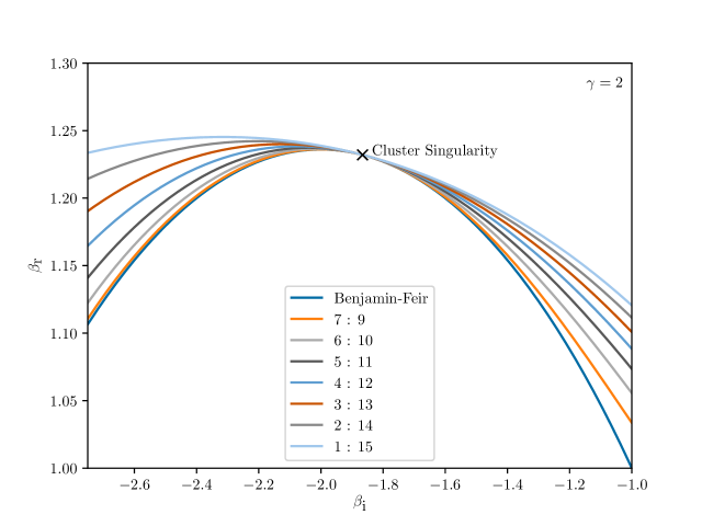
Figure 1: The Benjamin-Feir instability involving the $8:8$ cluster (dark blue) and the different saddle-node curves creating the unbalanced cluster solutions, $N_{1}\neq N_{2}$, in the $\beta_{\textrm{i}}$, $\beta_{\textrm{r}}$ plane with $\gamma=2$ and $N=16$. Each curve belongs to a particular cluster distribution $N_{1}:N_{2}$, and is obtained with numerical continuation using auto-07p [34, 35]. Note the position of the cluster singularity at $\beta_{\textrm{r}}=-(1-\sqrt{3}\gamma)/2\approx 1.23$, $\beta_{\textrm{i}}=(-\gamma-\sqrt{3})/2\approx-1.87$ as indicated.

The remainder of this article is organized as follows: In Sec. 2, we pass to a corotating frame and introduce the average amplitude $R$, the deviations from the average amplitude $r_{k}$, the deviations from the mean phase $\varphi_{k}$. Using this corotating system, we discuss how one can describe the dynamics in the center manifold, see Sec. 3. In Sec. 4, we derive the parameters for the dynamics of $x_{k}$. Detailed calculations are provided in Appendix C, for convenience. Based on the parameters in the center manifold, we study the bifurcations of 2-cluster states and the role of the cluster singularity in the center manifold, in Sec. 5. We conclude with a detailed discussion of our results and an outlook on future work. For a detailed mathematical analysis of the dynamics of 2-cluster states in the center manifold, see the companion paper Ref. [36].

2 Variable transformation into corotating frame

Notice that Eq. (2) is invariant under a rotation in the complex plane $W_{k}\rightarrow W_{k}\exp(i\phi)$. This invariance can be eliminated by choosing variables in a corotating frame, thus effectively reducing the dimensions of the system from $2N$ to $2N-1$.

In particular, we express the complex variables $W_{k}$ in log-polar coordinates $W_{k}=\exp(R_{k}+i\Phi_{k})$. Then Eq. (2) turns into

$$\dot{R} =1-e^{2R}\langle e^{2\mathbf{r}}\rangle+\operatorname{Re}\left(\left(\beta_{\textrm{r}}+i\beta_{\textrm{i}}\right)\left(\langle e^{\mathbf{z}}\rangle\langle e^{-\mathbf{z}}\rangle-1\right)\right)$$ (3a)

$$\dot{r}_{k} =-e^{2R}\widetilde{e^{2r_{k}}}+\operatorname{Re}\left(\left(\beta_{\textrm{r}}+i\beta_{\textrm{i}}\right)\left(\langle e^{\mathbf{z}}\rangle\widetilde{e^{-z_{k}}}\right)\right)$$ (3b)

$$\dot{\varphi}_{k} =-\gamma e^{2R}\widetilde{e^{2r_{k}}}+\operatorname{Im}\left(\left(\beta_{\textrm{r}}+i\beta_{\textrm{i}}\right)\left(\langle e^{\mathbf{z}}\rangle\widetilde{e^{-z_{k}}}\right)\right)$$ (3c)

with $k=1,\dots,N-1$, the abbreviations shown in Tab. 1 and the new coordinates summarized in Tab. 2 (see Appendix A for a derivation).

Table 1: Abbreviations

$\langle\mathbf{x}^{m}\rangle=1/N\sum_{j=1}^{N}x_{j}^{m}$	$\widetilde{x_{k}^{m}}=x_{k}^{m}-\langle\mathbf{x}^{m}\rangle$
$\langle e^{\mathbf{x}}\rangle=1/N\sum_{j=1}^{N}e^{x_{j}}$	$\widetilde{e^{x_{k}}}=e^{x_{k}}-\langle e^{\mathbf{x}}\rangle$

Table 2: Coordinate transformations

$R=\langle\mathbf{R}\rangle$	$r_{k}=\widetilde{R_{k}}$	$\Rightarrow\langle\mathbf{r}\rangle=0$
$\Phi=\langle\mathbf{\Phi}\rangle$	$\varphi_{k}=\widetilde{\Phi_{k}}$	$\Rightarrow\langle\boldsymbol{\varphi}\rangle=0$
	$z_{k}=r_{k}+i\varphi_{k}$	$\Rightarrow\langle\mathbf{z}\rangle=0$

Hereby, $\widetilde{\,\cdot\,}$ symbolizes the deviation from the ensemble mean $\langle\cdot\rangle$, and $R$ and $\Phi$ are the ensemble mean logarithmic amplitude and phase, respectively. The logarithmic amplitude and phase deviation of each oscillator from their averages are $r_{k}$ and $\varphi_{k}$. Notice that through this construction, the averages of these deviations vanish. Furthermore, bold face of a variable, e.g. $\mathbf{x}$, symbolizes the set of the respective ensemble variables $\left\{x_{1},x_{2},\dots,x_{N}\right\}$.
To simplify notation, $r_{k}+i\varphi_{k}$ is abbreviated by the complex variable $z_{k}$. The transformation into Eqs. (3a) to (3c) has the advantage that the resulting equations are independent of the mean phase $\Phi$. A change of $\Phi$ corresponds to a uniform phase shift of the whole ensemble in the complex plane, which in turn means that periodic orbits in the Stuart-Landau ensemble, Eq. (2), correspond to stationary solutions in the transformed system, Eqs. (3a) to (3c). Thus, we can ignore the mean phase $\Phi$ in our subsequent analysis.
Synchronized oscillations correspond to $R=0$, $r_{k}=0$, $\Phi=-\gamma t$ and $\varphi_{k}=0$. The stability of this equilibrium can be investigated using the eigenspectrum of the Jacobian evaluated at this point. Due to the $\mathbf{S}_{N}$-symmetry of the solution and the $\mathbf{S}_{N}$-equivariance of the governing equations, the Jacobian becomes block-diagonal, and thus has a degenerate eigenvalue spectrum [21, 15], see Appendix B:

• There is one singleton eigenvalue $\lambda_{1}=-2<0$, corresponding to an eigendirection affecting all oscillators identically. That is, this direction $\vec{v}_{1}$ shifts the amplitude of the synchronized motion but does not alter its symmetry.

• There is the eigenvalue $\lambda_{+}=-1-\beta_{\textrm{r}}+\sqrt{1-\beta_{\textrm{i}}^{2}-2\beta_{\textrm{i}}\gamma}=:-1-\beta_{\textrm{r}}+d$ which becomes zero at the Benjamin-Feir instability and is of geometric multiplicity $N-1$. The corresponding directions correspond to 2-cluster states, with each direction corresponding to one cluster distribution $N_{1}:N_{2}$. Up to conjugacy, we arrange here the units such that the first $N_{1}$ oscillators correspond to the same cluster. All 2-clusters with the same distribution but different assignments of the oscillators then belong to the same conjugacy class.

• Finally, there is the eigenvalue $\lambda_{-}=-1-\beta_{\textrm{r}}-d$ which is negative close to the synchronized solution, which has a geometric multiplicity of $N-1$ and whose eigendirections also have $\mathbf{S}_{N_{1}}\times\mathbf{S}_{N_{2}}$-symmetry.
  

Hereby, $d=\sqrt{1-\beta_{\textrm{i}}^{2}-2\beta_{\textrm{i}}\gamma}$ abbreviates the root of the discriminant where we assume $1-\beta_{\textrm{i}}^{2}-2\beta_{\textrm{i}}\gamma>0$, i.e. real $\lambda_{\pm}$. Notice that the Benjamin-Feir instability $\lambda_{+}=0$, alias $\beta_{\textrm{r}}=d-1$, i.e. the dark blue curve in Fig. 1, is of codimension one.

3 Center manifold reduction

In the following, we calculate an expansion to third order of the dynamics in the $(N-1)$-dimensional center manifold which corresponds to the Benjamin-Feir instability at $\lambda_{+}=0=-1-\beta_{\textrm{r}}+d$. In order to do so, it is useful to introduce the coordinates

$$x_{k} =\frac{-r_{k}+\frac{d+1}{\gamma^{\prime}}\varphi_{k}}{2d}$$ (4)

$$y_{k} =\frac{r_{k}+\frac{d-1}{\gamma^{\prime}}\varphi_{k}}{2d}$$ (5)

such that

$$r_{k} =\left(1-d\right)x_{k}+\left(1+d\right)y_{k}$$ (6)

$$\varphi_{k} =\gamma^{\prime}x_{k}+\gamma^{\prime}y_{k}.$$ (7)

Here we use the notations $\gamma^{\prime}=2\gamma+\beta_{\textrm{i}}$ and $d$ as defined above. See Appendix B for a derivation. The variables $x_{k}$ describe the dynamics in the $(N-1)$-dimensional center manifold tangent to $y_{k}=0\,\forall k$, while $y_{k}$ together with $R$ describe the dynamics in the stable manifold tangent to $x_{k}=0\,\forall k$.
Note that the center-manifold must be $\mathbf{S}_{N}$-invariant. In addition, the global restrictions $\langle\mathbf{r}\rangle=\langle\boldsymbol{\varphi}\rangle=0$ and thus $\langle\mathbf{x}\rangle=\langle\mathbf{y}\rangle=0$ must hold. Therefore, the general form of the center manifold up to quadratic order must follow

$$y_{k} =y_{k}\left(\mathbf{x}\right)=a\widetilde{x_{k}^{2}}+\mathcal{O}\left(x_{k}^{3}\right)$$ (8)

$$R =R\left(\mathbf{x}\right)=b\langle\mathbf{x}^{2}\rangle+\mathcal{O}\left(x_{k}^{3}\right)$$ (9)

with the coefficients $a=a\left(\beta_{\textrm{i}},\gamma\right)$ and $b=b\left(\beta_{\textrm{i}},\gamma\right)$. Here, we use the tangency of our coordinates $R$ and $y_{k}$, that is, $\left.\frac{\mathrm{d}}{\mathrm{d}x_{k}}R\right|_{\mathbf{x}=0}=0$ and $\left.\frac{\mathrm{d}}{\mathrm{d}x_{k}}y_{k}\right|_{\mathbf{x}=0}=0$. Since the Benjamin-Feir instability $\beta_{\textrm{r}}=d-1$ is of codimension one, the three-dimensional parameter space $(\beta_{\textrm{r}},\beta_{\textrm{i}},\gamma)$ becomes two-dimensional. The parameters in the center manifold thus only depend on $\beta_{\textrm{i}}$ and $\gamma$. By $\mathbf{S}_{N}$-equivariance, the reduced dynamics $\dot{x}_{k}$ in the center manifold, up to cubic order, must be of the form

$$\dot{x}_{k}=\lambda_{+}x_{k}+A\widetilde{x_{k}^{2}}+B\widetilde{x_{k}^{3}}+C\langle\mathbf{x}^{2}\rangle x_{k}+\mathcal{O}\left(x_{k}^{4}\right),$$ (10)

see also Refs. [10, 20], with the parameters $A=A\left(\beta_{\textrm{i}},\gamma\right)$ and $B=B\left(\beta_{\textrm{i}},\gamma\right)$ and $C=C\left(\beta_{\textrm{i}},\gamma\right)$.

4 Derivation of the parameters $a$, $b$, $A$, $B$ and $C$

In this section, we discuss the approach to calculate the coefficients $a$, $b$, $A$, $B$ and $C$ for the dynamics in the center manifold. See Appendix C for complete details.
First, we determine $b$. In particular we observe that

$$\dot{R}=\left(\frac{\mathrm{d}}{\mathrm{d}x_{k}}R\right)\,\dot{\mathbf{x}}=2b\langle\mathbf{x}\dot{\mathbf{x}}\rangle+\mathcal{O}\left(x_{k}^{5}\right)=2b\lambda_{+}\langle\mathbf{x}^{2}\rangle+\mathcal{O}\left(x_{k}^{3}\right)$$

holds. Since $\lambda_{+}=0$ at the bifurcation, $\dot{R}$ up to second order in $x_{k}$ must vanish. Therefore, expressing $z_{k}=r_{k}+i\varphi_{k}$ and $r_{k}$, $\varphi_{k}$ in terms of $x_{k}$ in Eq. (3a), we can compute $b$ by comparing the coefficients of the $\langle\mathbf{x}^{2}\rangle$: the terms in front of $\langle\mathbf{x}^{2}\rangle$ must thereby vanish. This allows us to estimate $b=b\left(\beta_{\textrm{i}},\gamma\right)$ as

$$b=\frac{1-d}{2}\left(\gamma^{\prime 2}+d^{2}+4d-5\right)$$ (11)

with $\gamma^{\prime}$ and $d$ as defined above.
Analogously, we can calculate $a$ using Eqs. 3a and 3b up to second order in $x_{k}$ and employing

$$\dot{y}_{k}=\left(\frac{\mathrm{d}}{\mathrm{d}x_{k}}y_{k}\right)\dot{x}_{k}=\mathcal{O}\left(x_{k}^{3}\right).$$

This means we can use $2d\dot{y}_{k}=\dot{r}_{k}+(d-1)/\gamma^{\prime}\dot{\varphi}_{k}$, substitute the $z_{k}$ with $x_{k}$ in Eqs. 3a and 3b and keep terms up to $\mathcal{O}\left(x_{k}^{2}\right)$. Comparing the coefficients in front of $\widetilde{x_{k}^{2}}$ then results in

$$a=\frac{\left(1-d\right)\left(\gamma^{\prime 2}+\left(1-d\right)^{2}\right)\left(3\left(d^{2}-1\right)+\gamma^{\prime 2}\right)}{8d^{2}\gamma^{\prime 2}}.$$ (12)

Finally, we can calculate $A$, $B$ and $C$ using

$$2d\dot{x}_{k} =-\dot{r}_{k}+\frac{d+1}{\gamma^{\prime}}\dot{\varphi}_{k}$$

$$=\lambda_{+}x_{k}+A\widetilde{x_{k}^{2}}+B\widetilde{x_{k}^{3}}+C\langle\mathbf{x}^{2}\rangle x_{k}.$$

Taking Eqs. 3b and 3c and the coefficients $a$ and $b$ obtained above, we can evaluate this equality up to cubic order, yielding the coefficients

$$A =\frac{\left(d-1\right)\left(\gamma^{\prime 2}+\left(1+d\right)^{2}\right)\left(\gamma^{\prime 2}-3\left(d-1\right)^{2}\right)}{4\gamma^{\prime 2}d}$$ (13)

$$B =-\frac{\left(d-1\right)^{2}\left(\gamma^{\prime 2}+\left(d-1\right)^{2}\right)\left(\gamma^{\prime 2}+\left(d+1\right)^{2}\right)\left(\gamma^{\prime 2}-2\gamma^{\prime}d+3\left(d^{2}-1\right)\right)\left(\gamma^{\prime 2}+2\gamma^{\prime}d+3\left(d^{2}-1\right)\right)}{16\gamma^{\prime 4}d^{3}}$$ (14)

$$C =\frac{\left(d-1\right)^{2}}{16d^{3}\gamma^{\prime 4}}\left(\vphantom{\int_{1}^{2}}\gamma^{\prime 8}-4\gamma^{\prime 6}\left(2d^{3}-7d^{2}+1\right)-2\gamma^{\prime 4}\left(8d^{5}+d^{4}-56d^{3}+22d^{2}+1\right)\right.$$

$$\left.-4\gamma^{\prime 2}\left(2d^{7}+5d^{6}-4d^{5}-13d^{4}+2d^{3}+11d^{2}-3\right)+9\left(d^{2}-1\right)^{4}\vphantom{\int_{1}^{2}}\right).$$ (15)

Together with $\lambda_{+}$, the expressions for $A$, $B$ and $C$ fully specify the dynamics in the center manifold based on the original parameters $\gamma$, $\beta_{\textrm{r}}$ and $\beta_{\textrm{i}}$. By rescaling time and $x_{k}$ in Eq. (10), the number of independent parameters can be reduced to two, see Ref. [36]. For simplicity, we use the unscaled equation as in Eq. (10) here.

5 Clustering and cluster singularities in the center manifold

As shown in Fig. 1 for $N=16$ oscillators, we observe a range of saddle-node bifurcations creating the different 2-cluster states. The expressions for $\lambda_{+}$, $A$, $B$ and $C$ above determine the corresponding parameter values in the center manifold. The respective $\lambda_{+}$ and $A$ values for the numerical curves shown in Fig. 1 are depicted in Fig. 2 as dashed curves.

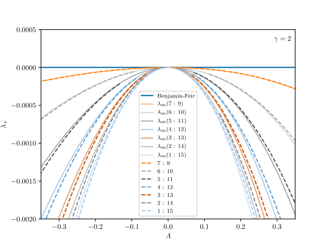
Figure 2: The Benjamin-Feir instability (blue, $\lambda_{+}=0$) and the different saddle-node curves creating the unbalanced cluster solutions in the $A$, $\lambda_{+}$ plane. The dashed curves belong to particular cluster distributions $N_{1}:N_{2}$ obtained by projecting the curves from the Stuart-Landau ensemble shown in Fig. 1 using the expressions for $\lambda_{+}(\beta_{\textrm{r}},\beta_{\textrm{i}},\gamma)=-1-\beta_{\textrm{r}}+d$, and $A(\beta_{\textrm{r}},\beta_{\textrm{i}},\gamma)$, cf. Eq. (13). The solid curves $\lambda_{\text{sn}}$ indicate the saddle-node bifurcations of the unbalanced cluster states obtained analytically in the center manifold, see Eq. (16). Note that close to the cluster singularity, where analytical expansions work best, numerical continuation fails due to the concentration of solutions in phase space.

Notice that the Benjamin-Feir curve corresponds to the line $\lambda_{+}=0$. Furthermore, we can derive the saddle-node curves creating unbalanced 2-cluster states in the center manifold analytically, see Appendix D. In particular,

$$\lambda_{\text{sn}}=\frac{A^{2}\left(1-\alpha\right)^{2}}{4\left(B\left(1-\alpha+\alpha^{2}\right)+C\alpha\right)}$$ (16)

for unbalanced cluster solutions, with $\alpha=N_{1}/N_{2}$. The respective analytical curves for $N=16$ are shown as solid curves in Fig. 2. Notice the close correspondence between the mapped bifurcation curves from the full system and the bifurcation curves determined in the center manifold. For less balanced solutions, the saddle-node curves obtained from the Stuart-Landau ensemble depart more strongly from the saddle-node curves calculated analytically in the center manifold. We expect this to be due to the cubic truncation of the flow in the center manifold, thus limiting its accuracy away from the Benjamin-Feir curve.

Note that to obtain the curves in Fig. 2, we fix $\gamma=2$ and vary $\beta_{\textrm{i}}$, $\beta_{\textrm{r}}$. We then use the expressions for $A(\beta_{\textrm{i}},\beta_{\textrm{r}})$, $B(\beta_{\textrm{i}},\beta_{\textrm{r}})$ and $C(\beta_{\textrm{i}},\beta_{\textrm{r}})$ to get the parameters in the center manifold. Thus the parameters $A$, $B$ and $C$ lie on a two-dimensional manifold. For the curves shown in Fig. 2, we furthermore use Eq. (16), yielding one-dimensional curves. The curves are, however, not exactly parabolas, since $B$ and $C$ vary in addition to $A$, which is not shown in Fig. 2. For all subsequent figures, we use the values of $C=-1$ and $B=-2/(2\sqrt{3}-3)$ at the cluster singularity for $\gamma=2$, which can be obtained analytically. See Ref. [36] p. 36 for a derivation.

Furthermore, from Fig. 2 we observe that $A=0$, in addition to $\lambda_{+}=0$, at the cluster singularity. This means that this codimension-two point is distinguished by vanishing quadratic dynamics in the center manifold, cf. Eq. 10. In addition, it serves as an organizing center for the saddle-node bifurcations of the unbalanced cluster states: At the saddle-node bifurcation, we have in the center manifold for a cluster state

$$x_{1}^{\ast}=-\frac{A\left(1-\alpha\right)}{2\left(B\left(1-\alpha+\alpha^{2}\right)+C\alpha\right)},$$

with $B<0$ and $C<0$ for the range of $\beta_{\textrm{i}}$, $\beta_{\textrm{r}}$ considered here (not shown), see Appendix D. This means that for negative $A$ values, the saddle-node curves occur at positive $x_{1}$, for positive $A$ values at negative $x_{1}$, and for $A=0$, at the cluster singularity, all saddle-node bifurcations occur at the synchronized solution $x_{k}=0$. This behavior can indeed be observed in the Stuart-Landau ensemble, see Fig. 6 of Ref. [32].

The unbalanced cluster states do, in general, not emerge as stable states from the saddle-node bifurcations. Rather, one of the two branches created at the saddle-node bifurcation is subsequently stabilized through transverse bifurcations involving 3-cluster solutions with symmetry $\mathbf{S}_{N_{1}}\times\mathbf{S}_{N_{2}}\times\mathbf{S}_{N_{3}}$, also called secondary branches [10]. For a more detailed discussion on secondary branches, see also Refs. [37, 28]
In order to explain this in more detail, we follow Ref. [37] Section 4. Note that each $N_{1}$ : $N_{2}$ 2-cluster solution is invariant under the action of the group $\mathbf{S}_{N_{1}}\times\mathbf{S}_{N_{2}}$. From this, it follows that one can block-diagonalise the Jacobian at the 2-cluster solutions $\mathbf{S}_{N_{1}}\times\mathbf{S}_{N_{2}}$. In doing so, one can calculate the $(N_{1}-1)$-degenerate eigenvalue $\mu_{1}$ describing the intrinsic stability of cluster $\Xi_{1}$, that is its stability against transverse perturbations. Note, however, that a cluster of size 1 cannot be broken up. Following Ref. [10] p. 23 and using isotypic decomposition, the eigenvalue $\mu_{1}$ can be expressed as

$$\mu_{1}=\left.\mathbf{J}_{11}\right|_{\Xi_{1}}-\left.\mathbf{J}_{12}\right|_{\Xi_{1}}.$$

Here, $\left.\mathbf{J}_{ij}\right|_{\Xi_{1}}$ denotes $\partial f_{i}/\partial x_{j}$, with the respective $x_{i}$ and $x_{j}$ in cluster $\Xi_{1}$ and $f_{i}$ being the right hand side of Eq. (10). Without loss of generality, we assume in the following that $\Xi_{1}$ is the cluster with the smaller number of oscillators, that is, $N_{1}\leq N_{2}$ or $\alpha\leq 1$. Evaluating the Jacobian, one obtains that the eigenvalue $\mu_{1}$ changes sign at

$$\lambda_{+,1}=\frac{\left(1-2\alpha\right)B-\alpha C}{\left(\alpha-2\right)^{2}B^{2}}A^{2}.$$ (17)

Analogously, the transverse stability of cluster $\Xi_{2}$ is described by

$$\mu_{2}=\left.\mathbf{J}_{11}\right|_{\Xi_{2}}-\left.\mathbf{J}_{12}\right|_{\Xi_{2}},$$

which changes sign at

$$\lambda_{+,2}=\frac{\left(\alpha-2\right)B-C}{\left(4\alpha^{2}-4\alpha+1\right)B^{2}}\alpha A^{2}.$$ (18)

Hereby, $\mu_{2}$ describes the intrinsic stability of cluster $\Xi_{2}$. Furthermore notice that for the balanced cluster, $\alpha=1$ and therefore $\lambda_{+,1}=\lambda_{+,2}$. Since both clusters contain an equal number of units, their respective intrinsic stabilities change simultaneously.

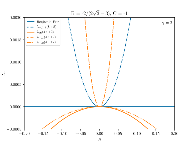
Figure 3: The bifurcation curves $\lambda_{+,1}$ ($\mu_{1}=0$, dotted orange) and $\lambda_{+,2}$ ($\mu_{2}=0$, dash-dotted orange) for the $4:12$ cluster state in the $A$, $\lambda_{+}$ plane and the parameters $B=-2/(2\sqrt{3}-3)$, $C=-1$. The saddle-node curve creating the $4:12$ cluster is shown as a solid orange curve. The Benjamin-Feir line is shown in blue, with the $\lambda_{+,1}=\lambda_{+,2}$ curve for the balanced $8:8$ cluster state depicted as a dotted blue curve. The $4:12$ cluster is stable in the two regions between the respective $\lambda_{+,1}=0$ and $\lambda_{+,2}=0$ curve. The balanced cluster state is stable above the dotted blue curve.

In Fig. 3, $\lambda_{\text{sn}}$, $\lambda_{+,1}$ and $\lambda_{+,2}$ are shown as solid, dotted and dash-dotted orange curves, respectively, for the $4:12$ 2-cluster state. The Benjamin-Feir instability, where the balanced cluster state is born, is drawn as a solid blue line at $\lambda_{+}=0$, and the transverse bifurcation curve $\lambda_{+,1}=\lambda_{+,2}$, where the balanced cluster state is stabilized, is drawn as a dotted blue curve. See Fig. 4 for the respective curves for a range of cluster distributions.

Fig. 3 can be interpreted as follows: Coming from negative $\lambda_{+}$ values, the unbalanced $4:12$ cluster state is born at $\lambda_{\text{sn}}(4:12)$ (solid orange). However, this 2-cluster state is unstable for the parameter values considered here: the cluster $\Xi_{1}$ with $4$ units is intrinsically unstable with $\mu_{1}>0$ and $\mu_{2}<0$. At the dotted orange curve, $\mu_{1}$ changes sign, rendering the $4:12$ cluster state stable. Subsequently, at the dash-dotted orange curve, $\mu_{2}$ changes sign, leaving the cluster $\Xi_{2}$ with 12 units intrinsically unstable and thus the $4:12$ cluster unstable.
The qualitatively same behavior can be observed for any cluster distribution $\alpha<1/2$, cf. Fig. 4, except for the most unbalanced state ($1:15$). There, cluster $\Xi_{1}$ cannot be intrinsically unstable, since it contains only one unit. This means that this cluster solution is born stable in its saddle-node bifurcation, and becomes unstable only at $\lambda_{2}$ when $\mu_{2}=0$. See also the bottom right plot in Fig. 4. In particular, $\lambda_{\text{sn}}=A^{2}/4B$ for $\alpha=0$, see Eq. (16), coincides with $\lambda_{+,1}=A^{2}/4B$ for $\alpha=0$, cf. Eq. (17). Furthermore, it is worth noting that the stable patches in parameter space overlap for different cluster distributions. This means that there is a multistability of different 2-cluster states.
Notice that these results are in close correspondence with the behavior observed in the full Stuart-Landau ensemble, compare, for example, Fig. 3 with Figs. 4b and 5b in Ref. [32].
$\lambda_{\text{sn}}$ and $\lambda_{+,1}$ are continuous functions of $\alpha$. For $N\rightarrow\infty$, this means that there are continuous bands of bifurcation curves: Going from $\lambda_{\text{sn}}(\alpha=0)=A^{2}/4B$ to $\lambda_{\text{sn}}(\alpha=1)=0$, there is band of saddle-node bifurcations creating the unbalanced cluster solutions. This band becomes infinitesimally thin at the cluster singularity $A=0$, giving it a bow-tie like shape. From $\lambda_{+,1}(\alpha=0)=A^{2}/4B$ to $\lambda_{+,1}(\alpha=1)=(-B-C)A^{2}/B^{2}$, the transverse bifurcations of the smaller cluster stretch from the saddle-node curve of the most unbalanced cluster state to the transverse bifurcations of the balanced cluster state where $\lambda_{+,1}$ is maximal, again yielding a bow-tie like shape in the $A$, $\lambda_{+}$ plane. Since $\lambda_{+,2}$ has a pole at $\alpha=1/2$, the interpretation is a bit more involved. First, for the balanced cluster state $\alpha=1$:

$$\lambda_{+,2}(\alpha=1)=(-B-C)A^{2}/B^{2}=\lambda_{+,1}(\alpha=1),$$

and thus $\lambda_{+,2}$ and $\lambda_{+,1}$ coincide. For the most unbalanced solution $\alpha=0$: $\lambda_{+,2}(\alpha=0)=0$. This means the larger cluster of the most unbalanced solution becomes unstable exactly when the balanced solution is born, that is, at the Benjamin-Feir instability $\lambda_{+}=0$. For intermediate $\alpha$ values, however, the $\lambda_{+,2}$ curve becomes steeper and infinitely steep at $\alpha=1/2$, with the tip reaching to the cluster singularity. This can also be observed in Fig. 4, where the parabola becomes thinner when going from the $6:10$ to the $5:11$ cluster states, and subsequently broadens again until the $1:15$ cluster. Altogether, the $\lambda_{+,2}$ curves fill out the half plane $\lambda_{+}\geq 0$ except the line $A=0$.
These three bow-tie like regions of $\lambda_{\text{sn}}$, $\lambda_{+,1}$ and $\lambda_{+,2}$ become infinitesimally thin and thus singular only at the cluster singularity $\lambda_{+}=0$, $A=0$.

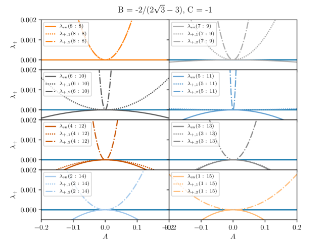
Figure 4: The theoretical bifurcation curves $\lambda_{+,1}$ ($\mu_{1}=0$, dotted) and $\lambda_{+,2}$ ($\mu_{2}=0$, dash-dotted) for the different cluster size distributions in the $A$, $\lambda_{+}$ plane and the parameters $B=-2/(2\sqrt{3}-3)$, $C=-1$. The saddle-node curves creating the unbalanced cluster solutions are represented as solid curves, which correspond to the shaded curves in Fig. 2 with the same color coding. The Benjamin-Feir line is shown in blue. The unbalanced cluster states are stable above the respective dotted curve and below the dash-dotted curve, except for the $1:15$ cluster, which is stable already at the saddle-node bifurcation. For the $2:14$ cluster, the dotted and solid curves do not coincide but lie very close in parameter space.

The bifurcation scenario can be better visualized by plotting $\lambda_{\text{sn}}$, $\lambda_{+,1}$ and $\lambda_{+,2}$ as a function of the cluster size $N_{1}/N$, see Fig. 5. It depicts the $\lambda_{+}$ values of the saddle-node bifurcations creating the 2-cluster states ($\lambda_{\text{sn}}$, blue) and of the two transverse bifurcations (Eqs. (17) and (18)) altering the stability of the 2-clusters, with $\lambda_{+,1}$ in green and $\lambda_{+,2}$ in orange.

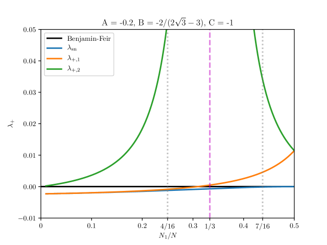
Figure 5: The bifurcation curves $\lambda_{\mathrm{sn}}$ (blue), $\lambda_{+,1}$ (orange) and $\lambda_{+,2}$ (green) for the different cluster-size distributions in the $\lambda_{+}$, $N_{1}/N$ plane with $A=-0.2$ and the parameters $B=-2/(2\sqrt{3}-3)$ and $C=-1$. The Benjamin-Feir instability is indicated by the black solid line. The dashed magenta line indicates the location where $\lambda_{+,2}$ diverges. The positions of the $4:12$ and $7:9$ cluster states are marked by the dotted vertical gray lines, see also Fig. 6 for the respective solution curves.

When increasing $\lambda_{+}$ coming from negative values, all cluster states with $N_{1}/N\neq 1/2$ are born in the saddle-node bifurcation $\lambda_{\text{sn}}$. Note that in fact two solutions for each $N_{1}/N$ are created this way. In Fig. 5, one can observe that for the most unbalanced state $N_{1}/N\rightarrow 0$, the transverse bifurcation stabilizing the smaller cluster $\lambda_{+,1}$ occurs immediately after the saddle-node bifurcation creating that cluster. This bifurcation alters the stability of one of the two solutions born in the saddle-node bifurcation, and in particular renders the smaller of the two clusters in that solution stable to transverse perturbations. For the parameter regime considered here ($A=-0.2$, $B=-2/(2\sqrt{3}-3)$ and $C=-1$), this solution is in fact stabilized at this bifurcation, that is for $\lambda_{+}>\lambda_{+,1}$.
For $N_{1}/N<1/3$, the respective 2-cluster solution remains stable until $\lambda_{+,2}$, where the larger cluster becomes unstable, thus rendering the whole solution unstable. This can, for example, be observed for the $4:12$ cluster-size distribution, see Fig. 6(top). There, the variable of one cluster, $x_{1}$, is plotted as a function of the bifurcation parameter $\lambda_{+}$. The blue dot on the left marks the saddle-node bifurcation wherein the two $4:12$ solutions are created. Initially, both solutions are unstable. At $\lambda_{+,1}$ (orange dot), one of them is stabilized, and at $\lambda_{+,2}$ (green dot), it is subsequently destabilized.

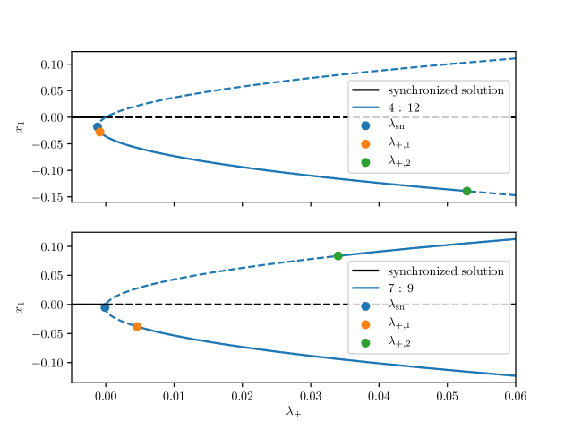
Figure 6: The variable $x_{1}$ of the $4:12$ cluster solution (top) and the $7:9$ cluster solution (bottom) as a function of the bifurcation parameter $\lambda_{+}$ with $A=-0.2$, and the parameters $B=-2/(2\sqrt{3}-3)$ and $C=-1$. Solid curves indicate that the solution is stable for the respective range of parameters, dashed curves represent unstable solutions. The points mark the $\lambda_{\mathrm{sn}}$ (blue), the $\lambda_{+,1}$ (orange) and the $\lambda_{+,2}$ (green) bifurcations. The synchronized solution $x_{i}=0\,\forall i$ is indicated by the black horizontal line. See also Fig. 5 for the locations of the $4:12$ and $7:9$ cluster in the $\lambda_{+}$, $N_{1}/N$ plane

For $N_{1}/N>1/3$, the scenario is different. There the solution that got stabilized at $\lambda_{+,1}$ remains stable for all $\lambda_{+}>\lambda_{+,1}$. The bifurcation $\lambda_{+,2}$ instead occurs at the second cluster solution created at the saddle-node bifurcation. This is illustrated more clearly in Fig. 6(bottom) for the $7:9$ cluster solution. One of the two solutions becomes stable at $\lambda_{+,1}$, marked by an orange dot and as discussed above. Since $N_{1}/N=7/16>1/3$, this solution remains stable for all $\lambda_{+}>\lambda_{+,1}$. The second solution (upper curve in the bottom part of Fig. 6) first passes the synchronized solution at the Benjamin-Feir bifurcation $\lambda_{+}=0$ and finally becomes stabilized at $\lambda_{+,2}$, marked by a green dot. $\lambda_{+,2}$ diverges at the pole $N_{1}/N=1/3$, separating the two scenarios shown in Fig. 6. There the bifurcation switches from the solution with negative $x_{1}$ (which, for $\lambda_{+}\rightarrow\infty$, diverges to $-\infty$) to the solution with positive $x_{1}$ (which, for $\lambda_{+}\rightarrow\infty$, diverges to $+\infty$).
Notice how for the cluster distribution $N_{1}/N=7/16$ the two 2-cluster solutions are bistable for $\lambda_{+}>\lambda_{+,2}$. That is, there exist two stable 2-cluster solutions with different $x_{1}$ but the same cluster size ratio $7:9$ that are both stable. This, in fact, has also been observed in the Stuart-Landau ensemble, see for example Fig. 6 in Ref. [32]. Note that the singularity of $\lambda_{+,2}$ at $N_{1}/N=1/3$ ($\alpha=1/2$) is independent of the parameters $A$, $B$ and $C$, see Eq. (18). This means that bistable solutions created as described above can in general only exist for $N_{1}/N>1/3$.

6 Conclusion and Outlook

In this paper, we showed how one can map a system of globally coupled Stuart-Landau oscillators onto the $(N-1)$-dimensional center manifold at the Benjamin-Feir instability. Thereby, we observed that the bifurcation curves at which 2-cluster solutions are born closely resemble their counterparts in the original oscillatory system. This allowed us to investigate a codimension-two point called cluster singularity, from which all these bifurcation curves emanate. In the center manifold, we saw that this point corresponds to a vanishing coefficient $A=0$ in front of the quadratic term of the equations of motion. Due to the reduced dynamics in this manifold, we were able to obtain stability boundaries for 2-cluster states analytically. This allows for the more detailed investigation of the bow-tie-shaped cascade of transverse bifurcations that govern the stability of these 2-cluster states, highlighting the role of the cluster singularity as an organizing center. The observed behavior is hereby independent of the oscillatory nature of each Stuart-Landau oscillator, but a result of the $\mathbf{S}_{N}$-equivariance of the full system. These findings may thus facilitate our understanding of this codimension-two point, and of clustering in general, even beyond oscillatory ensembles.
Through this reduction to the center manifold, we could calculate the bifurcation curves creating the cluster solutions ($\lambda_{\mathrm{sn}}$) and altering their stability ($\lambda_{+,1}$ and $\lambda_{+,2}$) analytically. This allowed us to investigate when stable 2-cluster solutions exist more systematically, and in particular revealed when different solutions with the same cluster-size distribution are bistable (cf. Fig. 6). The relative cluster size $N_{1}/N=1/3$ seems to be a general lower limit for such a bistable behavior. The bifurcation scenario of how states with different cluster size ratios $N_{1}/N$ are created is thereby different from the Eckhaus instability [38] in reaction-diffusion systems. There, solutions of different wavelengths are created through supercritial pitchfork bifurcations at the trivial solution and subsequently stabilized through a sequence of subcritical pitchfork bifurcations involving mixed-mode states. In our case, the different 2-cluster states are created in saddle-node bifurcations and stabilized at $\lambda_{+,1}$ at a single equivariant bifurcation point involving 3-cluster states. However, the detailed interaction between 2- and 3-cluster states still remains an open topic for future research.
Note that the cubic truncation of the flow in the center manifold has a gradient structure [36]. This means that we can assign an abstract potential to each of the cluster distributions for a particular set of parameters $\lambda_{+},A,B$ and $C$. Is there a particular cluster distribution with a minimal potential value? What is its role in the dynamics between these cluster distributions? The companion paper [36] addresses some of these dynamical questions.
Here, we fixed the parameter $\gamma=2$ in the full Stuart-Landau system, and varied the coupling parameters $\beta_{\textrm{r}}$, $\beta_{\textrm{i}}$. This restricts our analysis to a small region in parameter space. It is important to mention that for different parameter regimes, a qualitatively different behavior close to the cluster singularity might be observed [36].
As discussed in Sec. 2, the Stuart-Landau ensemble permits the transformation into a corotating frame. This turns limit-cycle dynamics into fixed-point dynamics and thus greatly facilitates the reduction onto the center manifold. For more general oscillatory ensembles, such as systems composed of van der Pol or Hogdkin-Huxley type units, the transformation to a corotating frame may be more cumbersome or not even possible. If the coupling between such units is of a global nature, we expect, however, that the nesting of bifurcation curves creating different cluster distributions, cf. Fig. 2, can also be observed in these systems.
This directly links to the fact that we focused on oscillatory dynamics in this article. An exciting further question is the possibility of equivalent dynamics, such as clustering and cluster singularities, in systems composed of bistable or excitable units.

Appendix A Variable transformation

Using log-polar coordinates $W_{k}=\exp\left(R_{k}+i\Phi_{k}\right)$, Eq. (2) turns into

$$\left(\dot{R}_{k}+i\dot{\Phi}_{k}\right)e^{R_{k}+i\Phi_{k}}=e^{R_{k}+i\Phi_{k}}-\left(1+i\gamma\right)e^{2R_{k}}e^{R_{k}+i\Phi_{k}}+\left(\beta_{\textrm{r}}+i\beta_{\textrm{i}}\right)\left(\langle e^{\mathbf{R}+i\mathbf{\Phi}}\rangle-e^{R_{k}+i\Phi_{k}}\right).$$

Dividing by $W_{k}$ this becomes

$$\dot{R}_{k}+i\dot{\Phi}_{k}=1-\left(1+i\gamma\right)e^{2R_{k}}+\left(\beta_{\textrm{r}}+i\beta_{\textrm{i}}\right)\left(\langle e^{\mathbf{R}+i\mathbf{\Phi}}\rangle e^{-R_{k}-i\Phi_{k}}-1\right).$$

We average over $k$ and separate real and imaginary parts. The mean amplitude $R$ and the mean phase $\Phi$ then satisfy

$$\dot{R} =1-\langle e^{2\mathbf{R}}\rangle+\operatorname{Re}\left(\left(\beta_{\textrm{r}}+i\beta_{\textrm{i}}\right)\left(\langle e^{\mathbf{R}+i\mathbf{\Phi}}\rangle\langle e^{-\mathbf{R}-i\mathbf{\Phi}}\rangle-1\right)\right)$$

$$\dot{\Phi} =-\gamma\langle e^{2\mathbf{R}}\rangle+\operatorname{Im}\left(\left(\beta_{\textrm{r}}+i\beta_{\textrm{i}}\right)\left(\langle e^{\mathbf{R}+i\mathbf{\Phi}}\rangle\langle e^{-\mathbf{R}-i\mathbf{\Phi}}\rangle-1\right)\right).$$

Substituting the variables listed in Tab. 2, one obtains $\langle\exp\left(2\mathbf{R}\right)\rangle=\langle\exp\left(2\mathbf{r}+2R\right)\rangle=\exp\left(2R\right)\langle\exp\left(2\mathbf{r}\right)\rangle$, and $\langle\exp\left(\mathbf{R}+i\mathbf{\Phi}\right)\rangle=\langle\exp\left(\mathbf{r}+R+i\boldsymbol{\varphi}+i\Phi\right)\rangle=\exp\left(R+i\Phi\right)\langle\exp\mathbf{z}\rangle$. Therefore

$$\dot{R} =1-e^{2R}\langle e^{2\mathbf{r}}\rangle+\operatorname{Re}\left(\left(\beta_{\textrm{r}}+i\beta_{\textrm{i}}\right)\left(\langle e^{\mathbf{z}}\rangle\langle e^{-\mathbf{z}}\rangle-1\right)\right)$$

$$\dot{\Phi} =-\gamma e^{2R}\langle e^{2\mathbf{r}}\rangle+\operatorname{Im}\left(\left(\beta_{\textrm{r}}+i\beta_{\textrm{i}}\right)\left(\langle e^{\mathbf{z}}\rangle\langle e^{-\mathbf{z}}\rangle-1\right)\right).$$

For the deviations $r_{k}=R_{k}-R$ and $\varphi_{k}=\Phi_{k}-\Phi$ one may write

$$\dot{r}_{k} =\dot{R}_{k}-\dot{R}$$

$$=1-e^{2R}e^{2r_{k}}+\operatorname{Re}\left(\left(\beta_{\textrm{r}}+i\beta_{\textrm{i}}\right)\left(\langle e^{\mathbf{z}}\rangle e^{-z_{k}}-1\right)\right)-\dot{R}$$

$$=-e^{2R}\widetilde{e^{2r_{k}}}+\operatorname{Re}\left(\left(\beta_{\textrm{r}}+i\beta_{\textrm{i}}\right)\left(\langle e^{\mathbf{z}}\rangle\widetilde{e^{-z_{k}}}\right)\right)$$

$$\dot{\varphi}_{k} =\dot{\Phi}_{k}-\dot{\Phi}$$

$$=-\gamma e^{2R}e^{2r_{k}}+\operatorname{Im}\left(\left(\beta_{\textrm{r}}+i\beta_{\textrm{i}}\right)\left(\langle e^{\mathbf{z}}\rangle e^{-z_{k}}-1\right)\right)-\dot{\Phi}$$

$$=-\gamma e^{2R}\widetilde{e^{2r_{k}}}+\operatorname{Im}\left(\left(\beta_{\textrm{r}}+i\beta_{\textrm{i}}\right)\left(\langle e^{\mathbf{z}}\rangle\widetilde{e^{-z_{k}}}\right)\right)$$

with the notations defined in table 1. The equations for $\dot{R}$, $\dot{r}_{k}$ and $\dot{\varphi}_{k}$ then constitute the corotating system Eqs. (3a) to (3c).

Appendix B Linearization

Linearizing the dynamics of the transformed system, Eqs. (3a) to (3c), at the equilibrium $R=0$, $r_{k}=\varphi_{k}=0$, $z_{k}=0$, and using the fact that $\langle\mathbf{r}\rangle=0$, $\langle\mathbf{z}\rangle=0$, see Tab. 2, one gets

$$\begin{pmatrix}\dot{R}\\ \dot{r}_{k}\\ \dot{\varphi}_{k}\end{pmatrix} =\begin{pmatrix}-2R\\ -2r_{k}-\operatorname{Re}\left(kz_{k}\right)\\ -2\gamma r_{k}-\operatorname{Im}\left(kz_{k}\right)\end{pmatrix}$$

$$=\begin{pmatrix}-2R\\ -\left(2+\beta_{\textrm{r}}\right)r_{k}+\beta_{\textrm{i}}\varphi_{k}\\ -\left(2\gamma+\beta_{\textrm{i}}\right)r_{k}-\beta_{\textrm{r}}\varphi_{k}\end{pmatrix}$$

$$=\begin{pmatrix}-2&0&0\\ 0&-2-\beta_{\textrm{r}}&\beta_{\textrm{i}}\\ 0&-2\gamma-\beta_{\textrm{i}}&-\beta_{\textrm{r}}\end{pmatrix}\cdot\begin{pmatrix}R\\ r_{k}\\ \varphi_{k}\end{pmatrix}=\mathbf{J}\cdot\begin{pmatrix}R\\ r_{k}\\ \varphi_{k}\end{pmatrix}.$$

The Jacobian thus has the eigenvalues

• Eigenvalue $\lambda_{1}=-2$ with eigenvector $\vec{v}_{1}=\left(1,\vec{0},\vec{0}\right)$.

and two eigenvalues of geometric multiplicity $N-1$ given by the eigendecomposition

$$\text{eig}\begin{pmatrix}[1.75]-2-\beta_{\textrm{r}}&\beta_{\textrm{i}}\\ -2\gamma-\beta_{\textrm{i}}&-\beta_{\textrm{r}}\end{pmatrix},$$

which gives

• the eigenvalue $\lambda_{+}=-1-\beta_{\textrm{r}}+\sqrt{1-\beta_{\textrm{i}}^{2}-2\beta_{\textrm{i}}\gamma}=-1-\beta_{\textrm{r}}+d$

• and the eigenvalue $\lambda_{-}=-1-\beta_{\textrm{r}}-\sqrt{1-\beta_{\textrm{i}}^{2}-2\beta_{\textrm{i}}\gamma}=-1-\beta_{\textrm{r}}-d$.

Here, we assume $1-\beta_{\textrm{i}}^{2}-2\beta_{\textrm{i}}\gamma>0$, that is real $\lambda_{\pm}$. For an analysis of the case $1-\beta_{\textrm{i}}^{2}-2\beta_{\textrm{i}}\gamma<0$, see Ref. [39]. The eigenvectors corresponding to these two eigenvalues can be obtained using

$$\left(\begin{pmatrix}[1.75]-2-\beta_{\textrm{r}}&\beta_{\textrm{i}}\\ -2\gamma-\beta_{\textrm{i}}&-\beta_{\textrm{r}}\end{pmatrix}-\lambda_{\pm}\mathbf{1}_{(N-1)\times(N-1)}\right)\vec{v}_{\pm}=\vec{0}.$$

For $\lambda_{+}$, one thus obtains

$$\begin{pmatrix}-1-d&\beta_{\textrm{i}}\\ -2\gamma-\beta_{\textrm{i}}&1-d\end{pmatrix}\vec{v}_{+} =\begin{pmatrix}-1-d&\beta_{\textrm{i}}\\ -2\gamma-\beta_{\textrm{i}}&1-d\end{pmatrix}\begin{pmatrix}r_{k}\\ \varphi_{k}\end{pmatrix}=\begin{pmatrix}\left(-1-d\right)r_{k}+\beta_{\textrm{i}}\varphi_{k}\\ \left(-2\gamma-\beta_{\textrm{i}}\right)r_{k}+\left(1-d\right)\varphi_{k}\end{pmatrix}=0.$$

Choosing

$$\varphi_{k}=(1+d)/\beta_{\textrm{i}}r_{k},$$ (A.1)

we get

$$\begin{pmatrix}\left(-1-d\right)r_{k}+\left(1+d\right)r_{k}\\ \left(-2\gamma-\beta_{\textrm{i}}\right)r_{k}+\left(1-d^{2}\right)/\beta_{\textrm{i}}r_{k}\end{pmatrix}=\begin{pmatrix}-\left(1+d\right)r_{k}+\left(1+d\right)r_{k}\\ -\left(2\gamma+\beta_{\textrm{i}}\right)r_{k}+\left(2\gamma+\beta_{\textrm{i}}\right)r_{k}\end{pmatrix}=\vec{0},$$

thus solving the equality above. The constraint Eq. (A.1), together with $\langle\mathbf{r}\rangle=\langle\boldsymbol{\varphi}\rangle=0$, defines an $(N-1)$-dimensional subspace of $\mathbb{R}^{2N-1}$.
For $\lambda_{-}$, one thus obtains

$$\begin{pmatrix}-1+d&\beta_{\textrm{i}}\\ -2\gamma-\beta_{\textrm{i}}&1+d\end{pmatrix}\vec{v}_{+} =\begin{pmatrix}-1+d&\beta_{\textrm{i}}\\ -2\gamma-\beta_{\textrm{i}}&1+d\end{pmatrix}\begin{pmatrix}r_{k}\\ \varphi_{k}\end{pmatrix}=\begin{pmatrix}\left(-1+d\right)r_{k}&\beta_{\textrm{i}}\varphi_{k}\\ \left(-2\gamma-\beta_{\textrm{i}}\right)r_{k}&\left(1+d\right)\varphi_{k}\end{pmatrix}.$$

Choosing

$$\varphi_{k}=(1-d)/\beta_{\textrm{i}}r_{k},$$ (A.2)

solves the conditions above. In particular,

$$\begin{pmatrix}\left(-1+d\right)r_{k}+\left(1-d\right)r_{k}\\ \left(-2\gamma-\beta_{\textrm{i}}\right)r_{k}+\left(1-d^{2}\right)/\beta_{\textrm{i}}r_{k}\end{pmatrix}=\begin{pmatrix}-\left(1-d\right)r_{k}+\left(1-d\right)r_{k}\\ -\left(2\gamma+\beta_{\textrm{i}}\right)r_{k}+\left(2\gamma+\beta_{\textrm{i}}\right)r_{k}\end{pmatrix}=\vec{0}.$$

The constraint Eq. (A.2), together with $\langle\mathbf{r}\rangle=\langle\boldsymbol{\varphi}\rangle=0$ define an $(N-1)$-dimensional subspace of $\mathbb{R}^{2N-1}$.
Now, one can define the eigencoordinates $x_{k}$ describing the dynamics in the space defined by the constraint Eq. (A.1), the center space of the bifurcation, and eigencoordinates $y_{k}$, describing the dynamics in the space defined by the constraint Eq. (A.2). These two sets of variables, together with $R$, can then be used to describe the full system.

Appendix C Parameter Derivation

In this section of the appendix, we derive expressions for the parameters $a$, $b$, $A$, $B$ and $C$ as a function of the parameters $\gamma$, $\beta_{\textrm{r}}$ and $\beta_{\textrm{i}}$ from the Stuart-Landau ensemble. Hereby, we will use the condition that $R$ and the $y_{k}$ are tangential, that is, $\left.\frac{\mathrm{d}}{\mathrm{d}x_{k}}R\right|_{\mathbf{x}=0}=0$ and $\left.\frac{\mathrm{d}}{\mathrm{d}x_{k}}y_{k}\right|_{\mathbf{x}=0}=0$.

C.1 $a$ and $b$

In order to calculate $a$ and $b$, it is useful to write out the following expressions

$$z_{k} =r_{k}+i\varphi_{k}$$

$$=\left(1-d\right)x_{k}+\left(1+d\right)y_{k}+i\left(\gamma^{\prime}x_{k}+\gamma^{\prime}y_{k}\right)$$

$$=\left(1-d+i\gamma^{\prime}\right)x_{k}+a\left(1+d+i\gamma^{\prime}\right)\widetilde{x_{k}^{2}}+\mathcal{O}\left(x_{k}^{3}\right)$$

$$z_{k}^{2} =\left(r_{k}+i\varphi_{k}\right)^{2}$$

$$=\left(\left(1-d\right)x_{k}+\left(1+d\right)y_{k}+i\left(\gamma^{\prime}x_{k}+\gamma^{\prime}y_{k}\right)\right)^{2}$$

$$=\left(\left(1-d+i\gamma^{\prime}\right)x_{k}+\left(1+d+i\gamma^{\prime}\right)y_{k}\right)^{2}$$

$$=\left(1-d+i\gamma^{\prime}\right)^{2}x_{k}^{2}+2a\left(1-d+i\gamma^{\prime}\right)\left(1+d+i\gamma^{\prime}\right)x_{k}\widetilde{x_{k}^{2}}+\mathcal{O}\left(x_{k}^{4}\right)$$

$$z_{k}^{3} =\left(r_{k}+i\varphi_{k}\right)^{3}$$

$$=\left(\left(1-d+i\gamma^{\prime}\right)x_{k}+\left(1+d+i\gamma^{\prime}\right)y_{k}\right)^{3}$$

$$=\left(1-d+i\gamma^{\prime}\right)^{3}x_{k}^{3}+\mathcal{O}\left(x_{k}^{4}\right)$$

where we used Eq (8) for $y_{k}$ and the notation $\gamma^{\prime}=2\gamma+\beta_{\textrm{i}}$. Similarly, we expand the following parts and keep terms up to cubic order:

$$e^{z_{k}} =1+z_{k}+\frac{z_{k}^{2}}{2}+\frac{z_{k}^{3}}{6}+\mathcal{O}\left(x_{k}^{4}\right)$$

$$e^{-z_{k}} =1-z_{k}+\frac{z_{k}^{2}}{2}-\frac{z_{k}^{3}}{6}+\mathcal{O}\left(x_{k}^{4}\right)$$

$$\langle e^{\mathbf{z}}\rangle =\langle 1+\mathbf{z}+\frac{\mathbf{z}^{2}}{2}+\frac{\mathbf{z}^{3}}{6}+\mathcal{O}\left(x_{k}^{4}\right)\rangle$$

$$=1+\frac{1}{2}\langle\mathbf{z}^{2}\rangle+\frac{1}{6}\langle{\mathbf{z}^{3}}\rangle+\mathcal{O}\left(x_{k}^{4}\right)$$

$$\widetilde{e^{-z_{k}}} =e^{-z_{k}}-\langle e^{-\mathbf{z}}\rangle$$

$$=1-z_{k}+\frac{z_{k}^{2}}{2}-\frac{z_{k}^{3}}{6}-1-\frac{1}{2}\langle\mathbf{z}^{2}\rangle+\frac{1}{6}\langle\mathbf{z}^{3}\rangle+\mathcal{O}\left(x_{k}^{4}\right)$$

$$=-z_{k}+\frac{1}{2}\widetilde{z_{k}^{2}}-\frac{1}{6}\widetilde{z_{k}^{3}}+\mathcal{O}\left(x_{k}^{4}\right)$$

$$\langle e^{\mathbf{z}}\rangle\langle e^{-\mathbf{z}}\rangle =\left(1+\frac{1}{2}\langle\mathbf{z}^{2}\rangle+\frac{1}{6}\langle{\mathbf{z}^{3}}\rangle\right)\left(1+\frac{1}{2}\langle\mathbf{z}^{2}\rangle-\frac{1}{6}\langle{\mathbf{z}^{3}}\rangle\right)+\mathcal{O}\left(x_{k}^{4}\right)$$

$$=1+\frac{1}{2}\langle\mathbf{z}^{2}\rangle+\frac{1}{6}\langle{\mathbf{z}^{3}}\rangle+\frac{1}{2}\langle\mathbf{z}^{2}\rangle-\frac{1}{6}\langle{\mathbf{z}^{3}}\rangle+\mathcal{O}\left(x_{k}^{4}\right)$$

$$=1+\langle\mathbf{z}^{2}\rangle+\mathcal{O}\left(x_{k}^{4}\right)$$

$$\langle e^{\mathbf{z}}\rangle\widetilde{e^{-z_{k}}} =\left(1+\frac{1}{2}\langle\mathbf{z}^{2}\rangle+\frac{1}{6}\langle{\mathbf{z}^{3}}\rangle\right)\left(-z_{k}+\frac{1}{2}\widetilde{z_{k}^{2}}-\frac{1}{6}\widetilde{z_{k}^{3}}\right)+\mathcal{O}\left(x_{k}^{4}\right)$$

$$=\left(1+\frac{1}{2}\langle\mathbf{z}^{2}\rangle\right)\left(-z_{k}+\frac{1}{2}\widetilde{z_{k}^{2}}-\frac{1}{6}\widetilde{z_{k}^{3}}\right)+\mathcal{O}\left(x_{k}^{4}\right)$$

$$=-z_{k}+\frac{1}{2}\widetilde{z_{k}^{2}}-\frac{1}{6}\widetilde{z_{k}^{3}}-\frac{1}{2}z_{k}\langle\mathbf{z}^{2}\rangle+\mathcal{O}\left(x_{k}^{4}\right).$$

With the expression for $R$, see Eq. (9), we can furthermore write

$$e^{2R} =1+2R+\mathcal{O}\left(x_{k}^{4}\right)$$

$$=1+2b\langle\mathbf{x}^{2}\rangle+\mathcal{O}\left(x_{k}^{4}\right)$$

$$e^{2r_{k}} =1+2r_{k}+2r_{k}^{2}+\frac{4}{3}r_{k}^{3}+\mathcal{O}\left(x_{k}^{4}\right)$$

$$\langle e^{2\mathbf{r}}\rangle =1+2\langle\mathbf{r}^{2}\rangle+\frac{4}{3}\langle\mathbf{r}^{3}\rangle+\mathcal{O}\left(x_{k}^{4}\right)$$

$$\widetilde{e^{2r_{k}}} =e^{2r_{k}}-\langle e^{2\mathbf{r}}\rangle$$

$$=2r_{k}+2\widetilde{r_{k}^{2}}+\frac{4}{3}\widetilde{r_{k}^{3}}+\mathcal{O}\left(x_{k}^{4}\right)$$

$$e^{2R}\langle e^{2\mathbf{r}}\rangle =\left(1+2b\langle\mathbf{x}^{2}\rangle\right)\left(1+2\langle\mathbf{r}^{2}\rangle+\frac{4}{3}\langle\mathbf{r}^{3}\rangle\right)+\mathcal{O}\left(x_{k}^{4}\right)$$

$$=1+2\langle\mathbf{r}^{2}\rangle+2b\langle\mathbf{x}^{2}\rangle+\frac{4}{3}\langle\mathbf{r}^{3}\rangle+\mathcal{O}\left(x_{k}^{4}\right)$$

$$e^{2R}\widetilde{e^{2r_{k}}} =\left(1+2b\langle\mathbf{x}^{2}\rangle\right)\left(2r_{k}+2\widetilde{r_{k}^{2}}+\frac{4}{3}\widetilde{r_{k}^{3}}\right)+\mathcal{O}\left(x_{k}^{4}\right)$$

$$=2r_{k}+2br_{k}\langle\mathbf{x}^{2}\rangle+2\widetilde{r_{k}^{2}}+\frac{4}{3}\widetilde{r_{k}^{3}}+\mathcal{O}\left(x_{k}^{4}\right).$$

Using these approximations, we can write for the dynamics of $R$ up to second order in $x_{k}$

$$\dot{R} =1-e^{2R}\langle e^{2\mathbf{r}}\rangle+\operatorname{Re}\left(\left(\beta_{\textrm{r}}+i\beta_{\textrm{i}}\right)\left(\langle e^{\mathbf{z}}\rangle\langle e^{-\mathbf{z}}\rangle-1\right)\right)$$

$$=1-\left(1+2\langle\mathbf{r}^{2}\rangle+2b\langle\mathbf{x}^{2}\rangle\right)+\operatorname{Re}\left(\left(\beta_{\textrm{r}}+i\beta_{\textrm{i}}\right)\left(1+\langle\mathbf{z}^{2}\rangle-1\right)\right)$$

$$=-2\langle\mathbf{r}^{2}\rangle-2b\langle\mathbf{x}^{2}\rangle+\operatorname{Re}\left(\left(\beta_{\textrm{r}}+i\beta_{\textrm{i}}\right)\langle\mathbf{z}^{2}\rangle\right)$$

$$=-2\left(1-d\right)^{2}\langle\mathbf{x}^{2}\rangle-2b\langle\mathbf{x}^{2}\rangle+\operatorname{Re}\left(\left(\beta_{\textrm{r}}+i\beta_{\textrm{i}}\right)\left(1-d+i\gamma^{\prime}\right)^{2}\right)\langle\mathbf{x}^{2}\rangle$$

$$=-2\left(1-d\right)^{2}\langle\mathbf{x}^{2}\rangle-2b\langle\mathbf{x}^{2}\rangle+\left(\beta_{\textrm{r}}\left(\left(1-d\right)^{2}-\gamma^{\prime 2}\right)-2\beta_{\textrm{i}}\left(\gamma^{\prime}\left(1-d\right)\right)\right)\langle\mathbf{x}^{2}\rangle$$

$$=-2\beta_{\textrm{r}}^{2}\langle\mathbf{x}^{2}\rangle-2b\langle\mathbf{x}^{2}\rangle+\left(\beta_{\textrm{r}}\left(\beta_{\textrm{r}}^{2}-\gamma^{\prime 2}\right)-2\left(\beta_{\textrm{r}}^{2}+2\beta_{\textrm{r}}\right)\beta_{\textrm{r}}\right)\langle\mathbf{x}^{2}\rangle$$

$$=-\left(2\beta_{\textrm{r}}^{2}-\beta_{\textrm{r}}\left(\beta_{\textrm{r}}^{2}-\gamma^{\prime 2}\right)+2\left(\beta_{\textrm{r}}^{2}+2\beta_{\textrm{r}}\right)\beta_{\textrm{r}}{-}2b\right)\langle\mathbf{x}^{2}\rangle$$

$$=-\left(6\beta_{\textrm{r}}^{2}+\beta_{\textrm{r}}^{3}+\beta_{\textrm{r}}\gamma^{\prime 2}{+}2b\right)\langle\mathbf{x}^{2}\rangle$$

Now, we use the tangential property of $R$. In particular, we can write

$$\dot{R}=\left(\frac{\mathrm{d}}{\mathrm{d}x_{k}}R\right)\,\dot{\mathbf{x}}=2b\langle\mathbf{x}\dot{\mathbf{x}}\rangle+\mathcal{O}\left(x_{k}^{5}\right)=2b\lambda_{+}\langle\mathbf{x}^{2}\rangle+\mathcal{O}\left(x_{k}^{3}\right).$$

At $\lambda_{+}=0$, $\dot{R}$ up to second order must vanish. This allows us to calculate $b$ by comparing the terms in front of $\langle\mathbf{x}^{2}\rangle$ in $\dot{R}$, yielding

$$\Rightarrow b =-\frac{\beta_{\textrm{r}}}{2}\left(\gamma^{\prime 2}+6\beta_{\textrm{r}}+\beta_{\textrm{r}}^{2}\right)$$

$$=\frac{1-d}{2}\left(\gamma^{\prime 2}+d^{2}+4d-5\right).$$

We can derive the expression for $a$ in a similar way. Here, we write out the dynamics of $y_{k}$ up to second order. This yields

$$2d\dot{y}_{k} =\dot{r}_{k}+\frac{d-1}{\gamma^{\prime}}\dot{\varphi}_{k}$$

$$=-\left(1+\left(d-1\right)\frac{\gamma}{\gamma^{\prime}}\right)e^{2R}\widetilde{e^{2r_{k}}}+\operatorname{Re}\left(\left(1-i\frac{d-1}{\gamma^{\prime}}\right)\left(\beta_{\textrm{r}}+i\beta_{\textrm{i}}\right)\left(\langle e^{\mathbf{z}}\rangle\widetilde{e^{-z_{k}}}\right)\right)$$

$$=-\left(1+\left(d-1\right)\frac{\gamma}{\gamma^{\prime}}\right)\left(2r_{k}+2\widetilde{r_{k}^{2}}\right)+\operatorname{Re}\left(\left(1-i\frac{d-1}{\gamma^{\prime}}\right)\left(\beta_{\textrm{r}}+i\beta_{\textrm{i}}\right)\left(-z_{k}+\frac{1}{2}\widetilde{z_{k}^{2}}\right)\right)$$

$$=-\left(1+\left(d-1\right)\frac{\gamma}{\gamma^{\prime}}\right)\left(2r_{k}+2\widetilde{r_{k}^{2}}\right)+\operatorname{Re}\left(\left(1-i\frac{d-1}{\gamma^{\prime}}\right)\left(\beta_{\textrm{r}}+i\beta_{\textrm{i}}\right)\left(-r_{k}-i\varphi_{k}+\frac{1}{2}{\widetilde{z_{k}^{2}}}\right)\right).$$

The term of the coupling constant and its parameters in front can be summarized by

$$\left(1-i\frac{\beta_{\textrm{r}}}{\gamma^{\prime}}\right)\left(\beta_{\textrm{r}}+i\beta_{\textrm{i}}\right) =\beta_{\textrm{r}}+\frac{\beta_{\textrm{i}}\beta_{\textrm{r}}}{\gamma^{\prime}}-i\left(\frac{\beta_{\textrm{r}}^{2}}{\gamma^{\prime}}-\beta_{\textrm{i}}\right)$$

$$=\beta_{\textrm{r}}-\frac{\beta_{\textrm{r}}^{3}+2\beta_{\textrm{r}}^{2}}{\gamma^{\prime 2}}-i\left(\frac{\beta_{\textrm{r}}^{2}}{\gamma^{\prime}}+\frac{\beta_{\textrm{r}}^{2}+2\beta_{\textrm{r}}}{\gamma^{\prime}}\right)$$

$$\beta_{\textrm{r}}\frac{\gamma}{\gamma^{\prime}} =\beta_{\textrm{r}}\frac{\gamma^{\prime}-\beta_{\textrm{i}}}{2\gamma^{\prime}}$$

$$=\frac{\beta_{\textrm{r}}}{2}+\frac{\beta_{\textrm{r}}^{3}+2\beta_{\textrm{r}}^{2}}{2\gamma^{\prime 2}}.$$

This simplifies the expression for $\dot{y}_{k}$ to

$$2d\dot{y}_{k} =-\left(2+\beta_{\textrm{r}}+\frac{\beta_{\textrm{r}}^{3}+2\beta_{\textrm{r}}^{2}}{\gamma^{\prime 2}}\right)\left(r_{k}+\widetilde{r_{k}^{2}}\right)$$

$$+\operatorname{Re}\left(\left(\beta_{\textrm{r}}-\frac{\beta_{\textrm{r}}^{3}+2\beta_{\textrm{r}}^{2}}{\gamma^{\prime 2}}-i\left(\frac{\beta_{\textrm{r}}^{2}}{\gamma^{\prime}}+\frac{\beta_{\textrm{r}}^{2}+2\beta_{\textrm{r}}}{\gamma^{\prime}}\right)\right)\left(-r_{k}-i\varphi_{k}+\frac{1}{2}{\widetilde{z_{k}^{2}}}\right)\right)$$

$$=-\left(2+\beta_{\textrm{r}}+\frac{\beta_{\textrm{r}}^{3}+2\beta_{\textrm{r}}^{2}}{\gamma^{\prime 2}}\right)\left(r_{k}+\widetilde{r_{k}^{2}}\right)$$

$$+\operatorname{Re}\left(\left(\beta_{\textrm{r}}-\frac{\beta_{\textrm{r}}^{3}+2\beta_{\textrm{r}}^{2}}{\gamma^{\prime 2}}-i\left(\frac{\beta_{\textrm{r}}^{2}}{\gamma^{\prime}}+\frac{\beta_{\textrm{r}}^{2}+2\beta_{\textrm{r}}}{\gamma^{\prime}}\right)\right)\left(-r_{k}-i\varphi_{k}+\frac{1}{2}\left(\left(1-d\right)^{2}-\gamma^{\prime 2}\right)\widetilde{x_{k}^{2}}+i\left(1-d\right)\gamma^{\prime}\widetilde{x_{k}^{2}}\right)\right)$$

$$=-\left(2+\beta_{\textrm{r}}+\frac{\beta_{\textrm{r}}^{3}+2\beta_{\textrm{r}}^{2}}{\gamma^{\prime 2}}\right)\left(r_{k}+\widetilde{r_{k}^{2}}\right)$$

$$+\left(\beta_{\textrm{r}}-\frac{\beta_{\textrm{r}}^{3}+2\beta_{\textrm{r}}^{2}}{\gamma^{\prime 2}}\right)\left(-r_{k}+\frac{1}{2}\left(\left(1-d\right)^{2}-\gamma^{\prime 2}\right)\widetilde{x_{k}^{2}}\right)-\left(\frac{\beta_{\textrm{r}}^{2}}{\gamma^{\prime}}+\frac{\beta_{\textrm{r}}^{2}+2\beta_{\textrm{r}}}{\gamma^{\prime}}\right)\left(\varphi_{k}-\left(1-d\right)\gamma^{\prime}\widetilde{x_{k}^{2}}\right)$$

$$=-2\left(\beta_{\textrm{r}}+1\right)r_{k}-\left(2+\beta_{\textrm{r}}+\frac{\beta_{\textrm{r}}^{3}+2\beta_{\textrm{r}}^{2}}{\gamma^{\prime 2}}\right)\widetilde{r_{k}^{2}}$$

$$+\frac{1}{2}\left(\beta_{\textrm{r}}-\frac{\beta_{\textrm{r}}^{3}+2\beta_{\textrm{r}}^{2}}{\gamma^{\prime 2}}\right)\left(\beta_{\textrm{r}}^{2}-\gamma^{\prime 2}\right)\widetilde{x_{k}^{2}}-2\left(\beta_{\textrm{r}}^{2}+\beta_{\textrm{r}}\right)\left(x_{k}+y_{k}\right){-}2\left(\beta_{\textrm{r}}^{2}+\beta_{\textrm{r}}\right)\beta_{\textrm{r}}\widetilde{x_{k}^{2}}$$

$$=-2\left(\beta_{\textrm{r}}+1\right)\left(-\beta_{\textrm{r}}x_{k}+\left(\beta_{\textrm{r}}+2\right)y_{k}\right)-\left(2+\beta_{\textrm{r}}+\frac{\beta_{\textrm{r}}^{3}+2\beta_{\textrm{r}}^{2}}{\gamma^{\prime 2}}\right)\beta_{\textrm{r}}^{2}\widetilde{x_{k}^{2}}$$

$$+\frac{1}{2}\left(\beta_{\textrm{r}}-\frac{\beta_{\textrm{r}}^{3}+2\beta_{\textrm{r}}^{2}}{\gamma^{\prime 2}}\right)\left(\beta_{\textrm{r}}^{2}-\gamma^{\prime 2}\right)\widetilde{x_{k}^{2}}-2\left(\beta_{\textrm{r}}^{2}+\beta_{\textrm{r}}\right)\left(x_{k}+y_{k}\right){-}2\left(\beta_{\textrm{r}}^{2}+\beta_{\textrm{r}}\right)\beta_{\textrm{r}}\widetilde{x_{k}^{2}}$$

$$=-4\left(\beta_{\textrm{r}}+1\right)^{2}y_{k}-\left(2+\beta_{\textrm{r}}+\frac{\beta_{\textrm{r}}^{3}+2\beta_{\textrm{r}}^{2}}{\gamma^{\prime 2}}\right)\beta_{\textrm{r}}^{2}\widetilde{x_{k}^{2}}$$

$$+\frac{1}{2}\left(\beta_{\textrm{r}}-\frac{\beta_{\textrm{r}}^{3}+2\beta_{\textrm{r}}^{2}}{\gamma^{\prime 2}}\right)\left(\beta_{\textrm{r}}^{2}-\gamma^{\prime 2}\right)\widetilde{x_{k}^{2}}{-}2\left(\beta_{\textrm{r}}^{2}+\beta_{\textrm{r}}\right)\beta_{\textrm{r}}\widetilde{x_{k}^{2}}$$

$$=-4\left(\beta_{\textrm{r}}+1\right)^{2}y_{k}{-\left(4+3\beta_{\textrm{r}}+\frac{\beta_{\textrm{r}}^{3}+2\beta_{\textrm{r}}^{2}}{\gamma^{\prime 2}}\right)}\beta_{\textrm{r}}^{2}\widetilde{x_{k}^{2}}$$

$$+\frac{1}{2}\left(\beta_{\textrm{r}}-\frac{\beta_{\textrm{r}}^{3}+2\beta_{\textrm{r}}^{2}}{\gamma^{\prime 2}}\right)\left(\beta_{\textrm{r}}^{2}-\gamma^{\prime 2}\right)\widetilde{x_{k}^{2}}$$

$$=-4\left(\beta_{\textrm{r}}+1\right)^{2}y_{k}{-\left(4+\frac{5}{2}\beta_{\textrm{r}}+\frac{3\beta_{\textrm{r}}^{3}+6\beta_{\textrm{r}}^{2}}{2\gamma^{\prime 2}}\right)\beta_{\textrm{r}}^{2}\widetilde{x_{k}^{2}}-\frac{1}{2}\left(\beta_{\textrm{r}}\gamma^{\prime 2}-\beta_{\textrm{r}}^{3}-2\beta_{\textrm{r}}^{2}\right)\widetilde{x_{k}^{2}}}$$

$$=-4\left(\beta_{\textrm{r}}+1\right)^{2}a\widetilde{x_{k}^{2}}{-\left(3+2\beta_{\textrm{r}}+\frac{3\beta_{\textrm{r}}^{3}+6\beta_{\textrm{r}}^{2}}{2\gamma^{\prime 2}}\right)\beta_{\textrm{r}}^{2}\widetilde{x_{k}^{2}}-\frac{1}{2}\beta_{\textrm{r}}\gamma^{\prime 2}\widetilde{x_{k}^{2}}}$$

$$=-4\left(\beta_{\textrm{r}}+1\right)^{2}a\widetilde{x_{k}^{2}}{-\frac{\beta_{\textrm{r}}}{2\gamma^{\prime 2}}\left(\gamma^{\prime 4}+6\beta_{\textrm{r}}\gamma^{\prime 2}+4\beta_{\textrm{r}}^{2}\gamma^{\prime 2}+3\beta_{\textrm{r}}^{4}+6\beta_{\textrm{r}}^{3}\right)\widetilde{x_{k}^{2}}}$$

$$=-4\left(\beta_{\textrm{r}}+1\right)^{2}a\widetilde{x_{k}^{2}}{-\frac{\beta_{\textrm{r}}}{2\gamma^{\prime 2}}\left(\gamma^{\prime 2}+\beta_{\textrm{r}}^{2}\right)\left(3\beta_{\textrm{r}}\left(\beta_{\textrm{r}}+2\right)+\gamma^{\prime 2}\right)\widetilde{x_{k}^{2}}}$$

Similar to $R$, the $y_{k}$ are tangential to the center manifold. This translates into the fact that

$$\dot{y}_{k}=\left(\frac{\mathrm{d}}{\mathrm{d}x_{k}}y_{k}\right)\dot{x}_{k}$$

vanishes up to second order in $x_{k}$. Therefore, comparing the terms in front of the $\widetilde{x_{k}^{2}}$ above yields

$$a ={-\frac{\beta_{\textrm{r}}\left(\gamma^{\prime 2}+\beta_{\textrm{r}}^{2}\right)\left(3\beta_{\textrm{r}}\left(\beta_{\textrm{r}}+2\right)+\gamma^{\prime 2}\right)}{8\left(\beta_{\textrm{r}}+1\right)^{2}\gamma^{\prime 2}}}$$

$$={\frac{\left(1-d\right)\left(\gamma^{\prime 2}+\left(1-d\right)^{2}\right)\left(3\left(d^{2}-1\right)+\gamma^{\prime 2}\right)}{8d^{2}\gamma^{\prime 2}}}.$$

C.2 $A$, $B$ and $C$

Finally, the coefficients $A$, $B$ and $C$ for the dynamics in the center manifold, cf. Eq. (10), can be obtained by expanding the dynamics of $x_{k}$,

$$2d\dot{x}_{k}=-\left(-1+\left(d+1\right)\frac{\gamma}{\gamma^{\prime}}\right)e^{2R}\widetilde{e^{2r_{k}}}+\operatorname{Re}\left(\left(-1-i\frac{d+1}{\gamma^{\prime}}\right)k\left(\langle e^{\mathbf{z}}\rangle\widetilde{e^{-z_{k}}}\right)\right)\,,$$ (C.2)

in powers of $x_{k}$: The terms in front of $\widetilde{x_{k}^{2}}$, $\widetilde{x_{k}^{3}}$ and $x_{k}\langle\mathbf{x}^{2}\rangle$ correspond to the coefficients $A$, $B$ and $C$, respectively. In order to do so, we approximate several terms as follows:

$$\langle e^{\mathbf{z}}\rangle\widetilde{e^{-z_{k}}} =-z_{k}+\frac{1}{2}\widetilde{z_{k}^{2}}-\frac{1}{6}\widetilde{z_{k}^{3}}-\frac{1}{2}z_{k}\langle\mathbf{z}^{2}\rangle+\mathcal{O}\left(x_{k}^{4}\right)$$

$$z_{k} =\left(1-d+i\gamma^{\prime}\right)x_{k}+a\left(1+d+i\gamma^{\prime}\right)\widetilde{x_{k}^{2}}+\mathcal{O}\left(x_{k}^{3}\right)$$

$$z_{k}^{2} =\left(1-d+i\gamma^{\prime}\right)^{2}x_{k}^{2}+2a\left(1-d+i\gamma^{\prime}\right)\left(1+d+i\gamma^{\prime}\right)x_{k}\widetilde{x_{k}^{2}}+\mathcal{O}\left(x_{k}^{4}\right)$$

$$\widetilde{z_{k}^{2}} =z_{k}^{2}-\langle\mathbf{z}^{2}\rangle$$

$$=\left(1-d+i\gamma^{\prime}\right)^{2}\widetilde{x_{k}^{2}}+2a\left(1-d+i\gamma^{\prime}\right)\left(1+d+i\gamma^{\prime}\right)\left(x_{k}\widetilde{x_{k}^{2}}-\langle\mathbf{x}\,\widetilde{\mathbf{x}^{2}}\rangle\right)+\mathcal{O}\left(x_{k}^{4}\right)$$

$$x_{k}\widetilde{x_{k}^{2}}-\langle\mathbf{x}\,\widetilde{\mathbf{x}^{2}}\rangle =x_{k}^{3}-x_{k}\langle\mathbf{x}^{2}\rangle-\langle\mathbf{x}^{3}\rangle+\langle\mathbf{x}\langle\mathbf{x}^{2}\rangle\rangle$$

$$=\widetilde{x_{k}^{3}}-x_{k}\langle\mathbf{x}^{2}\rangle$$

$$\widetilde{z_{k}^{2}} =\left(1-d+i\gamma^{\prime}\right)^{2}\widetilde{x_{k}^{2}}+2a\left(1-d+i\gamma^{\prime}\right)\left(1+d+i\gamma^{\prime}\right)\left(\widetilde{x_{k}^{3}}-x_{k}\langle\mathbf{x}^{2}\rangle\right)+\mathcal{O}\left(x_{k}^{4}\right)$$

$$z_{k}^{3} =\left(1-d+i\gamma^{\prime}\right)^{3}x_{k}^{3}+\mathcal{O}\left(x_{k}^{4}\right)$$

$$\widetilde{z_{k}^{3}} =\left(1-d+i\gamma^{\prime}\right)^{3}\widetilde{x_{k}^{3}}+\mathcal{O}\left(x_{k}^{4}\right)$$

$$z_{k}\langle\mathbf{z}^{2}\rangle =\left(\left(1-d+i\gamma^{\prime}\right)x_{k}+a\left(1+d+i\gamma^{\prime}\right)\widetilde{x_{k}^{2}}\right)$$

$$\cdot\langle\left(1-d+i\gamma^{\prime}\right)^{2}\mathbf{x}^{2}+2a\left(1-d+i\gamma^{\prime}\right)\left(1+d+i\gamma^{\prime}\right)\mathbf{x}\,\widetilde{\mathbf{x}^{2}}\rangle+\mathcal{O}\left(x_{k}^{4}\right)$$

$$=\left(\left(1-d+i\gamma^{\prime}\right)x_{k}+a\left(1+d+i\gamma^{\prime}\right)\widetilde{x_{k}^{2}}\right)\langle\left(1-d+i\gamma^{\prime}\right)^{2}\mathbf{x}^{2}\rangle+\mathcal{O}\left(x_{k}^{4}\right)$$

$$=\left(1-d+i\gamma^{\prime}\right)^{3}x_{k}\langle\mathbf{x}^{2}\rangle+\mathcal{O}\left(x_{k}^{4}\right).$$

Using these terms, we can write

$$\langle e^{\mathbf{z}}\rangle\widetilde{e^{-z_{k}}} =-z_{k}+\frac{1}{2}\widetilde{z_{k}^{2}}-\frac{1}{6}\widetilde{z_{k}^{3}}-\frac{1}{2}z_{k}\langle\mathbf{z}^{2}\rangle+\mathcal{O}\left(x_{k}^{4}\right)$$

$$=-\left(1-d+i\gamma^{\prime}\right)x_{k}-a\left(1+d+i\gamma^{\prime}\right)\widetilde{x_{k}^{2}}$$

$$+\frac{1}{2}\left(1-d+i\gamma^{\prime}\right)^{2}\widetilde{x_{k}^{2}}+a\left(1-d+i\gamma^{\prime}\right)\left(1+d+i\gamma^{\prime}\right)\left(\widetilde{x_{k}^{3}}-x_{k}\langle\mathbf{x}^{2}\rangle\right)$$

$$-\frac{1}{6}\left(1-d+i\gamma^{\prime}\right)^{3}\widetilde{x_{k}^{3}}$$

$$-\frac{1}{2}\left(1-d+i\gamma^{\prime}\right)^{3}x_{k}\langle\mathbf{x}^{2}\rangle$$

$$=-\left(1-d+i\gamma^{\prime}\right)x_{k}$$

$$+\left(\frac{1}{2}\left(1-d+i\gamma^{\prime}\right)^{2}-a\left(1+d+i\gamma^{\prime}\right)\right)\widetilde{x_{k}^{2}}$$

$$+\left(a\left(1-d+i\gamma^{\prime}\right)\left(1+d+i\gamma^{\prime}\right)-\frac{1}{6}\left(1-d+i\gamma^{\prime}\right)^{3}\right)\widetilde{x_{k}^{3}}$$

$$+\left(-\frac{1}{2}\left(1-d+i\gamma^{\prime}\right)^{3}-a\left(1-d+i\gamma^{\prime}\right)\left(1+d+i\gamma^{\prime}\right)\right)x_{k}\langle\mathbf{x}^{2}\rangle$$

$$e^{2R}\widetilde{e^{2r_{k}}} =\left(1+2b\langle\mathbf{x}^{2}\rangle\right)\left(2r_{k}+2\widetilde{r_{k}^{2}}+\frac{4}{3}\widetilde{r_{k}^{3}}\right)+\mathcal{O}\left(x_{k}^{4}\right)$$

$$=2r_{k}+{4}br_{k}\langle\mathbf{x}^{2}\rangle+2\widetilde{r_{k}^{2}}+\frac{4}{3}\widetilde{r_{k}^{3}}+\mathcal{O}\left(x_{k}^{4}\right)$$

$$r_{k} =\left(1-d\right)x_{k}+\left(1+d\right)y_{k}$$

$$=\left(1-d\right)x_{k}+\left(1+d\right)a\widetilde{x_{k}^{2}}$$

$$r_{k}^{2} =\left(1-d\right)^{2}x_{k}^{2}+2a\left(1-d\right)\left(1+d\right)x_{k}\widetilde{x_{k}^{2}}+\mathcal{O}\left(x_{k}^{4}\right)$$

$$r_{k}^{3} =\left(1-d\right)^{3}x_{k}^{3}+\mathcal{O}\left(x_{k}^{4}\right)$$

$$\widetilde{r_{k}^{2}} =r_{k}^{2}-\langle\mathbf{r}^{2}\rangle$$

$$=\left(1-d\right)^{2}\widetilde{x_{k}^{2}}+2a\left(1-d\right)\left(1+d\right)\left(\widetilde{x_{k}^{3}}-x_{k}\langle\mathbf{x}^{2}\rangle\right)$$

$$\widetilde{r_{k}^{3}} =\left(1-d\right)^{3}\widetilde{x_{k}^{3}}+\mathcal{O}\left(x_{k}^{4}\right)$$

$$e^{2R}\widetilde{e^{2r_{k}}} =2r_{k}+{4}br_{k}\langle\mathbf{x}^{2}\rangle+2\widetilde{r_{k}^{2}}+\frac{4}{3}\widetilde{r_{k}^{3}}+\mathcal{O}\left(x_{k}^{4}\right)$$

$$=2\left(1-d\right)x_{k}+2a\left(1+d\right)\widetilde{x_{k}^{2}}$$

$$+{4}b\left(1-d\right)x_{k}\langle\mathbf{x}^{2}\rangle$$

$$+2\left(1-d\right)^{2}\widetilde{x_{k}^{2}}+4a\left(1-d\right)\left(1+d\right)\left(\widetilde{x_{k}^{3}}-x_{k}\langle\mathbf{x}^{2}\rangle\right)$$

$$+\frac{4}{3}\left(1-d\right)^{3}\widetilde{x_{k}^{3}}+\mathcal{O}\left(x_{k}^{4}\right)$$

$$=2\left(1-d\right)x_{k}$$

$$+\left(2a\left(1+d\right)+2\left(1-d\right)^{2}\right)\widetilde{x_{k}^{2}}$$

$$+\left(4a\left(1-d\right)\left(1+d\right)+\frac{4}{3}\left(1-d\right)^{3}\right)\widetilde{x_{k}^{3}}$$

$$+\left({4}b\left(1-d\right)-4a\left(1-d\right)\left(1+d\right)\right)x_{k}\langle\mathbf{x}^{2}\rangle.$$

We can now insert the different orders of $x_{k}$ from $e^{2R}\widetilde{e^{2r_{k}}}$ and $\langle e^{\mathbf{z}}\rangle\widetilde{e^{-z_{k}}}$ in Eq. (C.2) (here, we use sympy [40] to solve for the coefficients), yielding

$$2d\dot{x}_{k} =\frac{\left(d-1\right)\left(\gamma^{\prime 2}+\left(1+d\right)^{2}\right)\left(\gamma^{\prime 2}-3\left(d-1\right)^{2}\right)}{2\gamma^{\prime 2}}\widetilde{x_{k}^{2}}$$

$$-\frac{\left(d-1\right)^{2}\left(\gamma^{\prime 2}+\left(d-1\right)^{2}\right)\left(\gamma^{\prime 2}+\left(d+1\right)^{2}\right)\left(\gamma^{\prime 2}-2\gamma^{\prime}d+3\left(d^{2}-1\right)\right)\left(\gamma^{\prime 2}+2\gamma^{\prime}d+3\left(d^{2}-1\right)\right)}{8\gamma^{\prime 4}d^{2}}\widetilde{x_{k}^{3}}$$

$$+\frac{\left(1-d\right)^{2}}{8d^{2}}\left(\vphantom{\int_{1}^{2}}\gamma^{\prime 4}-4\gamma^{\prime 2}\left(2d^{3}-7d^{2}+1\right)\right.$$

$$-2\left(8d^{5}+d^{4}-56d^{3}+22d^{2}+1\right)-\frac{4}{\gamma^{\prime 2}}\left(2d^{7}+5d^{6}-4d^{5}-13d^{4}+2d^{3}+11d^{2}-3\right)$$

$$\left.+\frac{9}{\gamma^{\prime 4}}\left(d^{2}-1\right)^{4}\vphantom{\int_{1}^{2}}\right)x_{k}\langle\mathbf{x}^{2}\rangle.$$

Reading off the coefficients then gives the parameters

$$A =\frac{\left(d-1\right)\left(\gamma^{\prime 2}+\left(1+d\right)^{2}\right)\left(\gamma^{\prime 2}-3\left(d-1\right)^{2}\right)}{4\gamma^{\prime 2}d}$$

$$B =-\frac{\left(d-1\right)^{2}\left(\gamma^{\prime 2}+\left(d-1\right)^{2}\right)\left(\gamma^{\prime 2}+\left(d+1\right)^{2}\right)\left(\gamma^{\prime 2}-2\gamma^{\prime}d+3\left(d^{2}-1\right)\right)\left(\gamma^{\prime 2}+2\gamma^{\prime}d+3\left(d^{2}-1\right)\right)}{16\gamma^{\prime 4}d^{3}}$$

$$C =\frac{\left(d-1\right)^{2}}{16d^{3}\gamma^{\prime 4}}\left(\vphantom{\int_{1}^{2}}\gamma^{\prime 8}-4\gamma^{\prime 6}\left(2d^{3}-7d^{2}+1\right)-2\gamma^{\prime 4}\left(8d^{5}+d^{4}-56d^{3}+22d^{2}+1\right)\right.$$

$$\left.-4\gamma^{\prime 2}\left(2d^{7}+5d^{6}-4d^{5}-13d^{4}+2d^{3}+11d^{2}-3\right)+9\left(d^{2}-1\right)^{4}\vphantom{\int_{1}^{2}}\right).$$

Appendix D 2-Cluster states in the center manifold

For 2-cluster states, we can take $N=N_{1}+N_{2}$ and write

$$\dot{x}_{k} =\lambda_{+}x_{k}+A\widetilde{x_{k}^{2}}+B\widetilde{x_{k}^{3}}+C\langle\mathbf{x}^{2}\rangle x_{k}+\mathcal{O}\left(x_{k}^{4}\right)$$

$$=\lambda_{+}x_{k}+A\left(x_{k}^{2}-\frac{1}{N}\left(N_{1}x_{1}^{2}+N_{2}x_{2}^{2}\right)\right)+B\left(x_{k}^{3}-\frac{1}{N}\left(N_{1}x_{1}^{3}+N_{2}x_{2}^{3}\right)\right)+\frac{C}{N}\left(N_{1}x_{1}^{2}+N_{2}x_{2}^{2}\right)x_{k}$$

with the constraint $k\in\left\{1,2\right\}$ and $N_{1}x_{1}+N_{2}x_{2}=0$, that is, $x_{2}=-(N_{1}/N_{2})x_{1}$. Note that $\dot{x}_{k}$ must vanish at the 2-cluster equilibria. The 2-cluster therefore satisfies

$$0 =\lambda_{+}x_{1}+A\left(x_{1}^{2}-\frac{1}{N}\left(N_{1}x_{1}^{2}+\frac{N_{1}^{2}}{N_{2}}x_{1}^{2}\right)\right)+B\left(x_{1}^{3}-\frac{1}{N}\left(N_{1}x_{1}^{3}-\frac{N_{1}^{3}}{N_{2}^{2}}x_{1}^{3}\right)\right)+\frac{C}{N}\left(N_{1}x_{1}^{2}+\frac{N_{1}^{2}}{N_{2}}x_{1}^{2}\right)x_{1}$$

$$=\lambda_{+}x_{1}+A\left(x_{1}^{2}-\frac{N_{1}}{N_{2}}x_{1}^{2}\right)+B\left(x_{1}^{3}-\frac{N_{1}\left(N_{2}-N_{1}\right)}{N_{2}^{2}}x_{1}^{3}\right)+\frac{CN_{1}}{N_{2}}x_{1}^{3}$$

$$=\lambda_{+}x_{1}+A\frac{N_{2}-N_{1}}{N_{2}}x_{1}^{2}+B\frac{N_{2}^{2}-N_{1}\left(N_{2}-N_{1}\right)}{N_{2}^{2}}x_{1}^{3}+\frac{CN_{1}}{N_{2}}x_{1}^{3},$$

and writing $\alpha=N_{1}/N_{2}$,

$$0 =\lambda_{+}x_{1}+A\left(1-\alpha\right)x_{1}^{2}+\left(B\left(1-\alpha+\alpha^{2}\right)+C\alpha\right)x_{1}^{3}.$$

This equation has the solutions $x_{1}=0,x_{2}=0$ and

$$x_{1}^{\pm} =\frac{1}{2\left(B\left(1-\alpha+\alpha^{2}\right)+C\alpha\right)}\left(-A\left(1-\alpha\right)\pm\sqrt{A^{2}\left(1-\alpha\right)^{2}-4\lambda_{+}\left(B\left(1-\alpha+\alpha^{2}\right)+C\alpha\right)}\right)$$

$$x_{2}^{\pm} =-(N_{1}/N_{2})x_{1}^{\pm}.$$

The saddle-node curves creating the 2-cluster solutions are thus parametrized by the vanishing discriminant

$$0 =A^{2}\left(1-\alpha\right)^{2}-4\lambda_{+}\left(B\left(1-\alpha+\alpha^{2}\right)+C\alpha\right)$$

$$\Rightarrow\lambda_{+}=\lambda_{\text{sn}} =\frac{A^{2}\left(1-\alpha\right)^{2}}{4\left(B\left(1-\alpha+\alpha^{2}\right)+C\alpha\right)}$$

for unbalanced cluster solutions, that is, $\alpha\neq 1$ or $N_{1}\neq N_{2}$. Thus, at the saddle-node bifurcation

$$x_{1}^{\pm}=x_{1}^{\ast}=-\frac{A\left(1-\alpha\right)}{2\left(B\left(1-\alpha+\alpha^{2}\right)+C\alpha\right)}.$$

References

- [1] Steven H. Strogatz. From Kuramoto to Crawford: Exploring the onset of synchronization in populations of coupled oscillators. Physica D: Nonlinear Phenomena, 143(1-4):1–20, 2000.
- [2] Vladimir García-Morales and Katharina Krischer. Normal-form approach to spatiotemporal pattern formation in globally coupled electrochemical systems. Physical Review E, 78(5):057201, 2008.
- [3] István Z. Kiss, Yumei Zhai, and John L. Hudson. Characteristics of cluster formation in a population of globally coupled electrochemical oscillators: an experiment-based phase model approach. Progress of Theoretical Physics Supplement, 161:99–106, 2006.
- [4] Wen Wang, István Z. Kiss, and J. L. Hudson. Experiments on arrays of globally coupled chaotic electrochemical oscillators: Synchronization and clustering. Chaos: An Interdisciplinary Journal of Nonlinear Science, 10(1):248–256, 2000.
- [5] Hamilton Varela, Carsten Beta, Antoine Bonnefont, and Katharina Krischer. A hierarchy of global coupling induced cluster patterns during the oscillatory H2-electrooxidation reaction on a Pt ring-electrode. Physical Chemistry Chemical Physics, 7(12):2429, 2005.
- [6] F. Plenge, H. Varela, and K. Krischer. Pattern formation in stiff oscillatory media with nonlocal coupling: a numerical study of the hydrogen oxidation reaction on Pt electrodes in the presence of poisons. Physical Review E, 72(6):066211, 2005.
- [7] Konrad Schönleber, Carla Zensen, Andreas Heinrich, and Katharina Krischer. Pattern formation during the oscillatory photoelectrodissolution of n-type silicon: Turbulence, clusters and chimeras. New Journal of Physics, 16(6):063024, 2014.
- [8] Minseok Kim, Matthias Bertram, Michael Pollmann, Alexander von Oertzen, Alexander S. Mikhailov, Harm Hinrich Rotermund, and Gerhard Ertl. Controlling chemical turbulence by global delayed feedback: Pattern formation in catalytic CO oxidation on Pt(110). Science, 292(5520):1357–1360, 2001.
- [9] Toby Elmhirst. Symmetry and emergence in polymorphism and sympatric speciation. PhD thesis, University of Warwick, Warwick, 2001.
- [10] Ian Stewart, Toby Elmhirst, and Jack Cohen. Symmetry-Breaking as an Origin of Species, pages 3–54. Bifurcation, Symmetry and Patterns. Birkhäuser Basel, 2003.
- [11] Koji Okuda. Variety and generality of clustering in globally coupled oscillators. Physica D: Nonlinear Phenomena, 63(3-4):424–436, 1993.
- [12] Naoko Nakagawa and Yoshiki Kuramoto. From collective oscillations to collective chaos in a globally coupled oscillator system. Physica D: Nonlinear Phenomena, 75(1-3):74–80, 1994.
- [13] Murad Banaji. Clustering in globally coupled oscillators. Dynamical Systems, 17(3):263–285, 2002.
- [14] Hiroaki Daido and Kenji Nakanishi. Aging and clustering in globally coupled oscillators. Physical Review E, 75(5):056206, 2007.
- [15] Wai Lim Ku, Michelle Girvan, and Edward Ott. Dynamical transitions in large systems of mean field-coupled Landau-Stuart oscillators: Extensive chaos and cluster states. Chaos: An Interdisciplinary Journal of Nonlinear Science, 25(12):123122, 2015.
- [16] Arkady Pikovsky and Michael Rosenblum. Dynamics of globally coupled oscillators: Progress and perspectives. Chaos: An Interdisciplinary Journal of Nonlinear Science, 25(9):097616, 2015.
- [17] Y. Kuramoto. Chemical Oscillations, Waves and Turbulence, volume 19 of Springer Series in Synergetics. Springer-Verlag Berlin Heidelberg, 1984.
- [18] Shinya Watanabe and Steven H. Strogatz. Integrability of a globally coupled oscillator array. Physical Review Letters, 70(16):2391–2394, 1993.
- [19] Shinya Watanabe and Steven H. Strogatz. Constants of motion for superconducting Josephson arrays. Physica D: Nonlinear Phenomena, 74(3-4):197–253, 1994.
- [20] Martin Golubitsky and Ian Stewart. Linear Stability, pages 33–57. Birkhäuser Basel, Basel, 2002.
- [21] Vincent Hakim and Wouter-Jan Rappel. Dynamics of the globally coupled complex Ginzburg-Landau equation. Physical Review A, 46(12):R7347–R7350, 1992.
- [22] T. Brooke Benjamin and J. E. Feir. The disintegration of wave trains on deep water part 1. Theory. Journal of Fluid Mechanics, 27(3):417–430, 1967.
- [23] Richard FitzHugh. Mathematical models of threshold phenomena in the nerve membrane. The Bulletin of Mathematical Biophysics, 17(4):257–278, 1955.
- [24] Balth. van der Pol. On relaxation-oscillations. The London, Edinburgh, and Dublin Philosophical Magazine and Journal of Science, 2(11):978–992, 1926.
- [25] Richard J. Field and Richard M. Noyes. Oscillations in chemical systems. iv. limit cycle behavior in a model of a real chemical reaction. The Journal of Chemical Physics, 60(5):1877–1884, 1974.
- [26] A. L. Hodgkin and A. F. Huxley. A quantitative description of membrane current and its application to conduction and excitation in nerve. The Journal of Physiology, 117(4):500–544, 1952.
- [27] Emilio Andreozzi, Ilaria Carannante, Giovanni D’Addio, Mario Cesarelli, and Pietro Balbi. Phenomenological models of nav1.5. a side by side, procedural, hands-on comparison between hodgkin-huxley and kinetic formalisms. Scientific Reports, 9(1):17493, 2019.
- [28] Ana Paula S. Dias and Ana Rodrigues. Secondary bifurcations in systems with all-to-all coupling. part ii. Dynamical Systems, 21(4):439–463, 2006.
- [29] D.G. Aronson, G.B. Ermentrout, and N. Kopell. Amplitude response of coupled oscillators. Physica D: Nonlinear Phenomena, 41(3):403–449, 1990.
- [30] Arkady Pikovsky, Michael Rosenblum, and Jürgen Kurths. Synchronization, pages 222–235. Cambridge University Press (CUP), 2001.
- [31] André Röhm, Kathy Lüdge, and Isabelle Schneider. Bistability in two simple symmetrically coupled oscillators with symmetry-broken amplitude- and phase-locking. Chaos: An Interdisciplinary Journal of Nonlinear Science, 28(6):063114, 2018.
- [32] Felix P. Kemeth, Sindre W. Haugland, and Katharina Krischer. Cluster singularity: the unfolding of clustering behavior in globally coupled Stuart-Landau oscillators. Chaos: An Interdisciplinary Journal of Nonlinear Science, 29(2):023107, 2019.
- [33] N. Nakagawa and Y. Kuramoto. Collective chaos in a population of globally coupled oscillators. Progress of Theoretical Physics, 89(2):313–323, 1993.
- [34] E. J. Doedel. AUTO: A program for the automatic bifurcation analysis of autonomous systems. In Congress numerantium, volume 30, 4 1981.
- [35] E. J. Doedel and X. J. Wang. AUTO-07P: Continuation and bifurcation software for ordinary differential equations. Technical report, Center for Research on Parallel Computing, California Institute of Technology, Pasadena CA 91125, 2007.
- [36] Bernold Fiedler, Sindre W. Haugland, Felix Kemeth, and Katharina Krischer. Global 2-cluster dynamics under large symmetric groups, 2020. arXiv preprint arXiv:2008.06944.
- [37] Paula S Dias and Ian Stewart. Secondary bifurcations in systems with all-to-all coupling. Proceedings of the Royal Society of London. Series A: Mathematical, Physical and Engineering Sciences, 459(2036):1969–1986, 2003.
- [38] Laurette S. Tuckerman and Dwight Barkley. Bifurcation analysis of the eckhaus instability. Physica D: Nonlinear Phenomena, 46(1):57–86, 1990.
- [39] Felix P. Kemeth. Symmetry Breaking in Networks of Globally Coupled Oscillators: From Clustering to Chimera States. PhD thesis, Technische Universität München, Garching, 4 2019.
- [40] Aaron Meurer, Christopher P. Smith, Mateusz Paprocki, Ondřej Čertík, Sergey B. Kirpichev, Matthew Rocklin, AMiT Kumar, Sergiu Ivanov, Jason K. Moore, Sartaj Singh, Thilina Rathnayake, Sean Vig, Brian E. Granger, Richard P. Muller, Francesco Bonazzi, Harsh Gupta, Shivam Vats, Fredrik Johansson, Fabian Pedregosa, Matthew J. Curry, Andy R. Terrel, Štěpán Roučka, Ashutosh Saboo, Isuru Fernando, Sumith Kulal, Robert Cimrman, and Anthony Scopatz. Sympy: Symbolic computing in python. PeerJ Computer Science, 3:e103, 2017.