Gaussian Closure Scheme in the Quasi–Linkage Equilibrium Regime of Evolving Genome Populations

Abstract

Describing the evolution of a population of genomes evolving in a complex fitness landscape is generally very hard. We here introduce an approximate Gaussian closure scheme to characterize analytically the statistics of a genomic population in the so-called Quasi–Linkage Equilibrium (QLE) regime, applicable to generic values of the rates of mutation or recombination and fitness functions. The Gaussian approximation is illustrated on a short-range fitness landscape with two far away and competing maxima. It unveils the existence of a phase transition from a broad to a polarized distribution of genomes as the strength of epistatic couplings is increased, characterized by slow coarsening dynamics of competing allele domains. Results of the closure scheme are corroborated by numerical simulations.

I Introduction

Understanding how genomes stochastically change as a result of selection, mutation and sexual recombination processes is the central goal of evolutionary biology. While the case of selection acting independently on the different alleles, a regime called linkage equilibrium (LE), has been intensively studied describing the dynamics of a population of genomes evolving in a complex fitness landscape, characterized by multiple and strong couplings between alleles, remains a formidable challenge to population geneticists and statistical physicists Barton and de Vladar (2009). An important step beyond LE was done by Kimura in ’65 Kimura (1965) for a 2-loci system at high recombination rate $r$, a regime called quasi-linkage equilibrium (QLE). Recently, Neher and Shraimann extensively studied the same regime for multi-loci systems Neher and Shraiman (2011). In QLE the distribution of genomes in a population may reach a stationary regime in which the pairwise correlations between alleles are weak, proportional to the fitness coupling between these two alleles and to the inverse $1/r$ of the recombination rate. To what extent this regime remains present or valid at low recombination remains unclear.

The irruption of massive sequence data, following the rapid drop in sequencing cost, has brought additional interest to such questions. It is now legitimate to ask how relevant parameters (such as mutation or recombination rates, or the full fitness function) can be extracted from sequences. An example can be found in Neher and Leitner (2010), where the effective recombination rate of HIV was inferred based on a specific model for intra-patient evolution. The large–$r$ relation between correlations and epistatic coupling was also used to infer fitness contribution from data in Gao et al. (2019). However, incorporating evolutionary models into inverse statistical approaches, such as the ones developed for extracting structural and functional constraints from protein sequences Cocco et al. (2018) remains a largely open issue so far.

The daunting complexity of the relationship between fitness determinants and the statistical properties of genomic data calls for the design of accurate and practical approximation schemes. We hereafter consider a Gaussian closure scheme for the hierarchy of moments of the allele distributions. Various other proposals of general, approximate frameworks in the context of the dynamics of populations can be found in literature, e.g. Turelli and Barton (1994); Bürger (2000) and, more recently, Jain and Stephan (2017); Barghi et al. (2020). In particular Barton and Turelli introduced general recursion equations for multi-locus cumulants, which they apply to the case of interchangeable additive traits under strong selection Turelli and Barton (1994). While our approximation is less general than Barton and Turelli’s as it relies on the first and second moments only, it is a practical tool to deal with cases in which traits are neither interchangeable, i.e loci contribute differently to fitness, nor additive, as found in predominantly epistatic fitness landscapes.

As we will show, our Gaussian scheme allows us to bypass the large–$r$ expansion made in Kimura (1965); Neher and Shraiman (2011), and study the existence of QLE in a larger range of recombination and mutation rates. We apply our approximation to a specific fitness model in which two very different genomes have maximal and equal fitness values, and with short-range (along the genome) and strong epistatic contributions. As the mutation and recombination rates are varied a phase transition takes place within the QLE regime, which separates a disordered (paramagnetic) regime in which alleles are not polarized along any of the two genomes and a polarized (ferromagnetic) phase in which, after coarsening of alternating allele domains, one of the two genomes dominates in the population.

II Model for the stochastic evolution of a genome population

We consider a population of $N$ individuals, whose genomes $\textbf{s}^{(k)}=\{s_{0}^{(k)},s^{(k)}_{1},...,s^{(k)}_{L-1}\}$, with $k=1,...N$, include $L$ loci. Each locus $i=0,...,L-1$ can carry one out of two states (alleles), $s_{i}=\pm 1$. Genomes stochastically evolve over time $t$, due to selection, mutation and sexual recombination processes. We will denote by $\langle G\rangle(t)$ the average of any function $G({\bf s})$ over the genomes in the population at time $t$,

$$\braket{G}(t)=\frac{1}{N}\sum_{k}G\big{(}\textbf{s}^{(k)}\big{)}\ .$$ (1)

Selection. The number of individuals carrying sequence s grow inside the population according to the growth rate $F(\textbf{s})$, called fitness. The fitness function can be expanded in terms of the state variables,

$$F(\textbf{s})=F_{0}+\sum_{i}f_{i}\,s_{i}+\sum_{i<j}f_{ij}\,s_{i}\,s_{j}\ ,$$ (2)

where we neglect all the interactions of order equal to, or higher than three, and consider only local ($f_{i}$) and pairwise epistatic ($f_{ij}$) contributions. In practice, selection can be enforced in simulations as follows. Time is discretize into very small time steps $\Delta t$. At each time step selection results in a re-sampling of the available sequences according to a Boltzmann probability distribution with the weights defined by the fitness of each sequence, i.e. $p(\textbf{s}_{k})\propto{e^{F(\textbf{s}_{k})}}$ with $k=1,\dots,N$. We make sure that the population size, $N$, is kept fixed. Note that the constant $F_{0}$ plays no role and can be set to zero.

Mutation. Each state $s_{i}$ can flip its value, $s_{i}\to-s_{i}$, with rate (probability per unit of time) $\mu$. This rate is supposed to be uniform across loci $i$ and individuals.

Recombination. For each infinitesimal time interval $\Delta t$, with probability $r\Delta t/N_{pairs}$, a pair of individuals is chosen uniformly at random among all $N_{pairs}=\frac{1}{2}N(N-1)$ pairs, where $r$ is the recombination rate. These two individuals, called mother (m) and father (f), undergo outcrossing. Two new genotypes $\bf s$, $\bf s^{\prime}$ are formed by inheriting some loci from the genome of the mother, $\textbf{s}^{(m)}$, and the complement from the father with genome $\textbf{s}^{(f)}$. This process is described by the inheritance vector $\bm{\xi}=\{\xi_{i}\}$, with $\xi_{i}\in\{0,1\}$: the $i$-th allele of $\bf s$ is inherited from the mother if $\xi_{i}=1$ and from the father if $x_{i}=0$, and vice versa for $\bf s^{\prime}$. Hence, $s_{i}=s_{i}^{(m)}\,\xi_{i}+s_{i}^{(f)}\,(1-\xi_{i})$. The inheritance vector $\bm{\xi}$ is itself stochastic, and we denote by $C({\bm{\xi}})$ its probability. In the following, we will need to consider in particular the recombination correlation $c_{ij}\equiv\sum_{\bm{\xi}}C(\bm{\xi})\left[\xi_{i}(1-\xi_{j})+(1-\xi_{i})\xi_{j}\right]$, which represents the probability that loci $i$ and $j$ take their alleles $s_{i}$ and $s_{j}$ from different parents.

III Equations for the spin moments and closure scheme

The above dynamical processes entirely characterizes the stochastic evolution of the genome population. We will hereafter track the first two cumulants of the allele distribution over time,

$$\chi_{i}(t)=\langle s_{i}\rangle(t)\ ,\quad\chi_{ij}(t)=\langle s_{i}s_{j}\rangle(t)-\langle s_{i}\rangle(t)\langle s_{j}\rangle(t)\ ,$$ (3)

where the averages are computed over the genomes in the population at time $t$. Note that $\chi_{ii}(t)=1-\chi_{i}(t)^{2}$.

In the infinite size limit ($N\to\infty$), these moments obey deterministic first-order differential equations derived by Neher and Shraimann Neher and Shraiman (2011). Unfortunately these equations are not closed, as they involve higher-order moments in the allele variables. Our closure scheme consists in replacing these high-order moments with the values they would have if the distribution of the $s_{i}$’s were Gaussian, i.e. in neglecting all cumulants of order $\geq 3$. Qualitatively speaking, we assume a quasi-species-like scenario, in which the population is distributed around an average sequence given by $\bm{\chi}=\{\chi_{0},...,\chi_{L-1}\}$, with some fluctuations encoded in the covariance matrix of components $\chi_{ij}$. As both the average sequence and the covariance matrix depend on $t$, the approximation offers an analytical way to track the genome population in the course of evolution.

Within the Gaussian closure scheme we obtain the following set of $\frac{1}{2}L(L+1)$ coupled equations (with the convention $f_{ij}=f_{ji}$ if $i\neq j$ and $f_{ii}=0$), see Appendix A for derivation,

$$\dot{\chi}_{i}=\sum_{j}\chi_{ij}\left[f_{j}+\sum_{k}f_{jk}\chi_{k}-2f_{ij}\chi_{i}\right]-2\mu\,\chi_{i}\,,$$ (4)

and, for $i\neq j$,

$$\dot{\chi}_{ij} = -2\chi_{ij}\left[f_{j}\chi_{j}+f_{i}\chi_{i}\right]+\sum_{k\neq l}\chi_{ik}\,f_{kl}\,\chi_{jl}$$ (5)

$$- 2\chi_{ij}\sum_{k}\big{[}f_{ki}(\chi_{ik}+\chi_{i}\chi_{k})+f_{kj}(\chi_{jk}+\chi_{j}\chi_{k})\big{]}$$

$$+ 2f_{ij}\chi_{ij}\left[\chi_{ij}+2\chi_{i}\chi_{j}\right]-(4\mu+rc_{ij})\chi_{ij}\,.$$

III.1 Case of additive fitness

In the absence of any epistatic contribution to the fitness ($f_{ij}=0$ for all $i\neq j$), equation (5) for the second cumulant becomes $\dot{\chi}_{ij}=-(2f_{j}\chi_{j}+2f_{i}\chi_{i}+4\mu+rc_{ij})\chi_{ij}$, whose only fixed point is $\chi_{ij}=0$. Hence, recombination and mutations contribute to erase correlation between alleles, a scenario known as LE. The resulting value of the first moment is root of $f_{i}(1-\chi_{i}^{2})-2\mu\chi_{i}=0$; it smoothly interpolates between $\chi_{i}=2f_{i}/\mu$ at large mutation rate and $\chi_{i}=\text{sign}(f_{i})$ at vanishingly small $\mu$, which corresponds to monoclonality.

III.2 Case of random epistatic contributions: comparison to numerical simulations and strong recombination theory of QLE

As a first, empirical test of the quantitative accuracy of the Gaussian closure scheme we have simulated the stochastic evolution of a population of $N=10,000$ individuals. The fitness is defined by eqn (2), with random quenched local biases $f_{i}$ and epistatic couplings $f_{ij}$ drawn from a normal law with zero mean and variances equal to, respectively, $\Delta h^{2}$ and $\Delta f^{2}$. In Fig. 1 we show the scatter plot of the correlations obtained from simulations once stationarity is reached, $\chi_{ij}^{sim}$, vs. the solutions of (5), $\chi_{ij}$, for one generic sample. The Gaussian Ansatz correctly estimates small correlations, but is less accurate for large ones (in absolute values). It performs substantially better that the QLE approximation in the high-$r$ regime from Neher and Shraiman (2011), see red and blue dots and caption of Fig. 1 for details. In the inset of Fig. 1 we show the normalized mean squared error,

$$\epsilon=\sqrt{\displaystyle{\sum_{i<j}\big{|}\chi_{ij}-\chi^{sim}_{ij}\big{|}^{2}}\big{/}{\displaystyle{\sum_{i<j}\big{(}\chi_{ij}^{sim}\big{)}^{2}}}}\,,$$ (6)

as a function of $\Delta f$ in the Gaussian closure scheme. For these values of $\mu$ and $r$, we obtain decent estimates of the correlations as long as $\Delta f$ is not too large, see below.

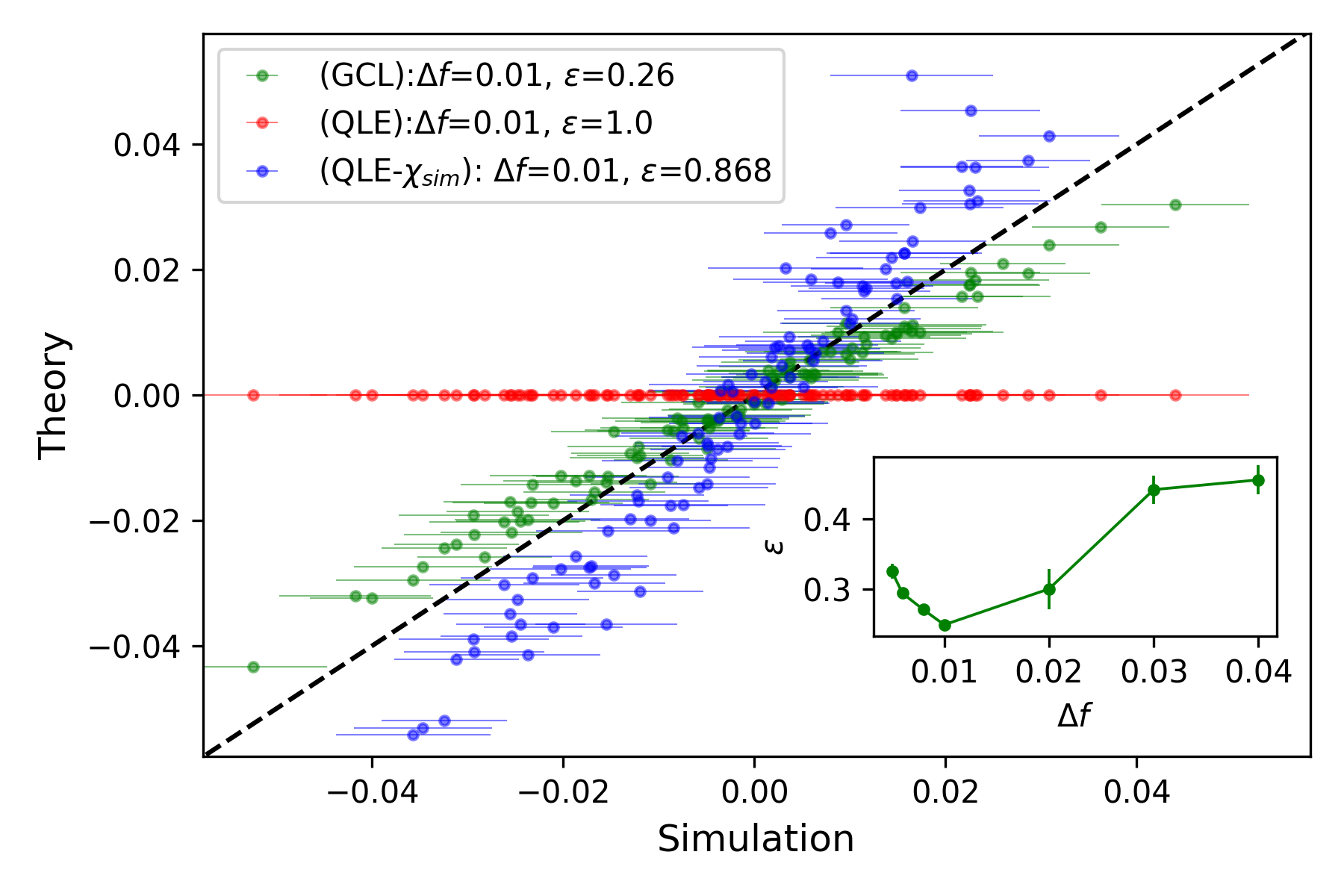
Figure 1: Scatter plot of the correlations $\chi_{ij}$ obtained from the Gaussian closure scheme (Eqs. (4, 5)) (green) or their estimates from large–$r$ QLE theory (red: eqs. (27) of Neher and Shraiman (2011) for $\chi_{i}$ and $\chi_{ij}$; blue: same equations for $\chi_{ij}$ only, replacing the $\chi_{i}$’s with their actual values $\chi_{i}^{sim}$ found in simulation to account for mutations) vs. simulations of finite populations (averaged over 500 generations once stationarity is reached) in the case of fully epistatic fitness landscape, see text and parameters in figure. Theoretical estimates of $\chi_{ij}$ are obtained by solving the dynamical system (4, 5) within Euler approximation. Inset: relative error $\epsilon$ (6) as a function of the standard deviation $\Delta f$ of the epistatic couplings. Parameters: $L=15$, $\mu=0.08$, $r=0.85$, $\Delta h=0.01$ and $c_{ij}=\frac{1}{2}(1-\rho^{|i-j|})$ with $\rho=0.6$.

III.3 Self-consistent condition for the validity of the Gaussian closure

The computation of high order moments, which should vanish if the Gaussian approximation were exact, is sketched in Appendix B. We obtain in particular that moments of order $k$ are, for large $k(\leq L)$, bounded from above by $\sim\exp(\log k!!+\frac{k}{2}\log|\chi_{ij}|+O(\log L))$, where $|\chi_{ij}|$ denotes the order of magnitude of the 2-point correlations. Due to the asymptotic scaling of the double factorial, we conclude that $k^{th}$ moment decays exponentially with $k$ if

$$L\times|\chi_{ij}|<1\ .$$ (7)

In other words, the total amount of correlations that a site, say, $i$, ‘receives’ from the $(L-1)$ other sites, say, $j$ should be smaller than unity. This condition is sufficient and not necessary, as possible cancellation between terms of opposite signs have not been considered. It is in addition self-consistent as it must be fulfilled by the 2-point correlations computed within the Gaussian closure scheme. We will check that condition (7) is satisfied for the non-trivial model with epistatic couplings studied below.

IV Study of short-range epistatic model

We now consider stochastic evolution under a fitness model with strong and spatially organized epistatic couplings,

$$F(\textbf{s})=f\sum_{i=0}^{L-1}s_{i}\,s_{i+1}\ ,$$ (8)

where $s_{L}\equiv s_{0}$ (circular chromosome); $F$ is maximal for the two genomes $(-,-,...,-)$ and $(+,+,...,+)$. As for the recombination correlation, we will choose either $c_{ij}=\frac{1}{2}(1-\rho^{|i-j|})$, which increases from 0 to $\frac{1}{2}$ with the distance between the loci, or $c_{ij}=\frac{1}{2}$ independently of the sites $i\neq j$. While the latter choice is less realistic, it does not affect the qualitative behavior of the model as we will see below, and allows for mathematical analysis in the $N\to\infty$ limit. Our goal is to understand how the distribution of alleles in the population change as a function of $\mu$ and $r$. Hereafter, we define $x=\mu/f$, $y=r/(2f)$.

V Paramagnetic phase

Due to the absence of local biases ($f_{i}=0$), the fitness is left unchanged by a global flip of all loci, $s_{i}\to-s_{i}$. In the absence of spontaneous symmetry breaking and in agreement with (4), we assume that $\chi_{i}=0$ for all sites $i$. In this paramagnetic (PM) regime we look for a stationary and translation–invariant solution, $\chi_{ij}=\chi^{st}\big{(}d=|i-j|\big{)}$, to the coupled equations (5) owing to the periodic boundary conditions in (8). We find that, for all $d\geq 1$,

$$\chi^{st}(d+1)\!\!\! = \!\!\!\big{[}3\chi^{st}(1)+a\big{]}\chi^{st}(d)-\chi^{st}(1)^{2}\,\delta_{d,1}$$

$$- \frac{1}{2}\sum_{k=0}^{d-1}\sum_{s=0,1}\chi^{st}(k+s)\chi^{st}(d-k-1+s)$$

$$- \sum_{k=1}^{\infty}\sum_{s=0,1}\chi^{st}(k+s)\chi^{st}(d+k+1-s)\,,$$

where $a\equiv 2x+\frac{y}{2}$. To obtain a tractable approximation for $\chi^{st}(d)$ we further neglect all the terms with $k>d+1$ in the r.h.s. (last term) of (V). This approximation is based on the assumption that correlations decay quickly with the distance between loci, which will be checked a posteriori. Within this approximation the generating function $\tilde{\chi}^{st}(z)\equiv\displaystyle{\sum_{d\geq 0}\chi^{st}(d)z^{d}}$ is given by $G(z,u=0)$, where

$$G(z,u)=\frac{z(3\chi^{st}(1)+a+4u)\pm\sqrt{\Delta(z,u)}}{1+z^{2}}\,,$$ (10)

and $\Delta(z,u)=z^{2}(3\chi^{st}(1)+a+4u)^{2}+(1+z^{2})[(1-u)^{2}-2z(1-u)(2\chi^{st}(1)+4u+a)-2z^{2}\chi^{st}(1)(\chi^{st}(1)+2u)]$; notice that $\chi^{st}(1)=d\tilde{\chi}^{st}(z)/dz|_{z=0}$.

The singularities of $\tilde{\chi}^{st}(z)$ control the asymptotic behaviour of $\chi^{st}(d)$ Flajolet and Sedgewick (2009). More precisely, if $\tilde{\chi}^{st}(z)$ behaves as $(z_{c}-z)^{\beta}$ close to its singularity, then

$$\chi^{st}(d)\sim z_{c}^{-d}\,d^{-(\beta+1)}$$ (11)

for large $d$; here, the square root in (10) entails that $\beta=\frac{1}{2}$. To locate the singularity $z_{c}$ we identify the roots of $\Delta(z,0)$. As $\Delta$ is a polynomial of degree 4, it has two real roots and two conjugated complex roots, with modulus lower than 1. For values of $a>a_{c}\simeq 2.542$, there is one appropriate value for $\chi^{st}(1)$, which depends on $a$, such that the two complex roots merge on the real axis. This choice, accompanied by a change of sign in front of $\sqrt{\Delta}$ in (10), removes the corresponding singularity and ensures that the radius of convergence $z_{c}$ of $G$ is larger than unity, as required for the exponential decay of $\chi^{st}(d)$. The radius of convergence $z_{c}$ and the corresponding value of $\chi^{st}(1)$ are shown as functions of $a$ in Fig. 2; for large $a$, $z_{c}\simeq\frac{a}{2}\gg 1$. Therefore the correlation function $\chi^{st}(d)$ (11) decays very quickly with $d$, as expected for large mutation or recombination rates. For $a<a_{c}$ removal of the singularity corresponding to the small-modulus complex roots is not possible, indicating the presence of a qualitatively different regime we will study below.

Figure 2: Radius of convergence $z_{c}$ (left) and corresponding value of $\chi^{st}(1)$ (right) vs. $a=2x+\frac{y}{2}$ in the PM regime. Red dotted lines show the large–$a$ asymptotic behaviours.

We compare in Fig. 3 the average values of the correlations $\chi_{ij}$ obtained by simulating a finite population with the ones computed above using the generating function $\tilde{\chi}^{st}(z)$. The agreement is excellent for small $d$, and more difficult to assess at large $d$ due to the finite-size and noise effects in the simulations.

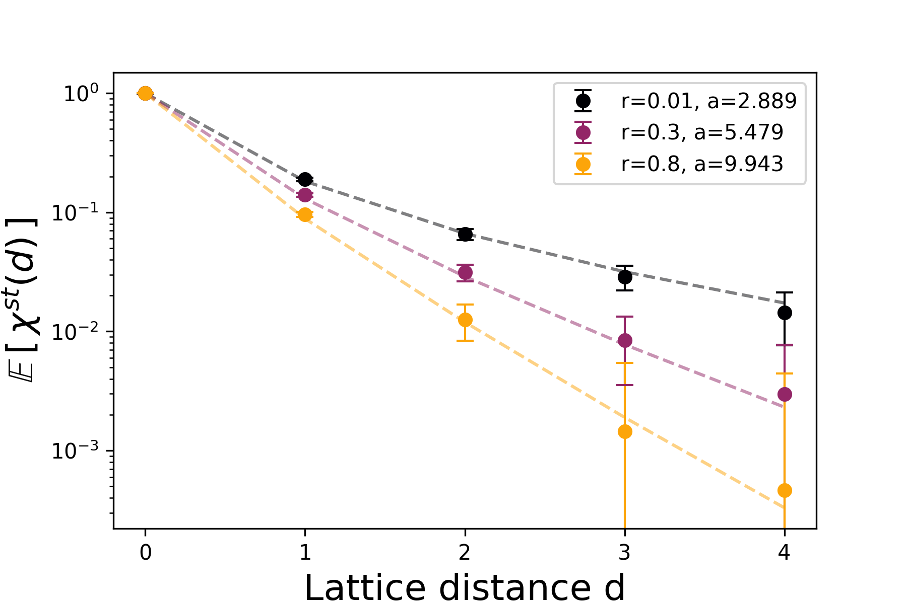
Figure 3: Average correlations in the PM phase for a finite population (dots) against the value computed from Gaussian closure eqs. (4, 5) (dashed lines) through Euler approximation, for three recombination rates $r$. Parameters: $f=0.028,L=50,\mu=0.03,N=10^{4}$, $c_{ij}=\frac{1}{2}(1-\rho^{|i-j|})$ with $\rho=0.6$; results are obtained by averaging over $5000$ generations.

VI Critical line and spontaneous symmetry breaking

The condition $a>a_{c}$ is necessary for the correlations to decay with distance, but it is not sufficient for the paramagnetic phase to hold. To investigate the onset of non-zero $\chi_{i}$’s, we study the stability of the PM solution found above against small fluctuations of the frequencies $\chi_{i}$. To do so we linearize eqn. (4) at fixed correlations $\chi_{ij}=\chi^{st}(|i-j|)$, and obtain $\dot{\chi}_{i}=-2f\sum_{j}{\cal M}_{ij}\chi_{j}$, where the entries of the $\cal M$ matrix read

$${\cal M}_{ij}=\big{[}2\chi^{st}(1)+x\big{]}\delta_{ij}+\\ -\frac{1}{2}\bigg{[}\chi^{st}(|j-i+1|)+\chi^{st}(|j-i-1|)\bigg{]}\,,$$ (12)

Being $\cal M$ translation invariant it can be diagonalized by Fourier plane waves, and its eigenvalues $\lambda_{n}$ are given by, for $n=0,1,...,L=1$,

$$\lambda_{n}=2\chi^{st}(1)+x+\\ -\left[2\,\mathrm{Re}\,\tilde{\chi}^{st}\left(e^{-i\frac{2\pi}{L}n}\right)-1\right]\cos\left(\frac{2\pi n}{L}\right)\,,$$ (13)

where $\tilde{\chi}$ is the generating function in (10). The PM phase is stable as long as all the eigenvalues $\lambda_{n}$ are strictly positive. The vanishing of $\lambda_{0}$, the lowest eigenvalue of $\cal M$, thus defines the boundary of the paramagnetic phase. This critical line is shown in the $(x,y)$ plane in Fig. 4, and corresponds to the condition $x=2\tilde{\chi}^{st}(1)-2\chi^{st}(1)-1$. We compared our analytical results, valid for $N\to\infty$, with simulations for a large but finite population size. We report the values of the Edward-Anderson overlap $q=\frac{1}{L}\sum_{i}\chi_{i}^{2}$ in Fig. 4. We observe that $q$ takes very low values to the right of the critical line where the paramagnetic phase is predicted to be stable, which justifies a posteriori our approximation above. To the left of the critical line, $q>0$, which signals the onset of a ferromagnetic phase; the mutation rate is too weak to ensure that the average values of the $s_{i}$’s are zero.

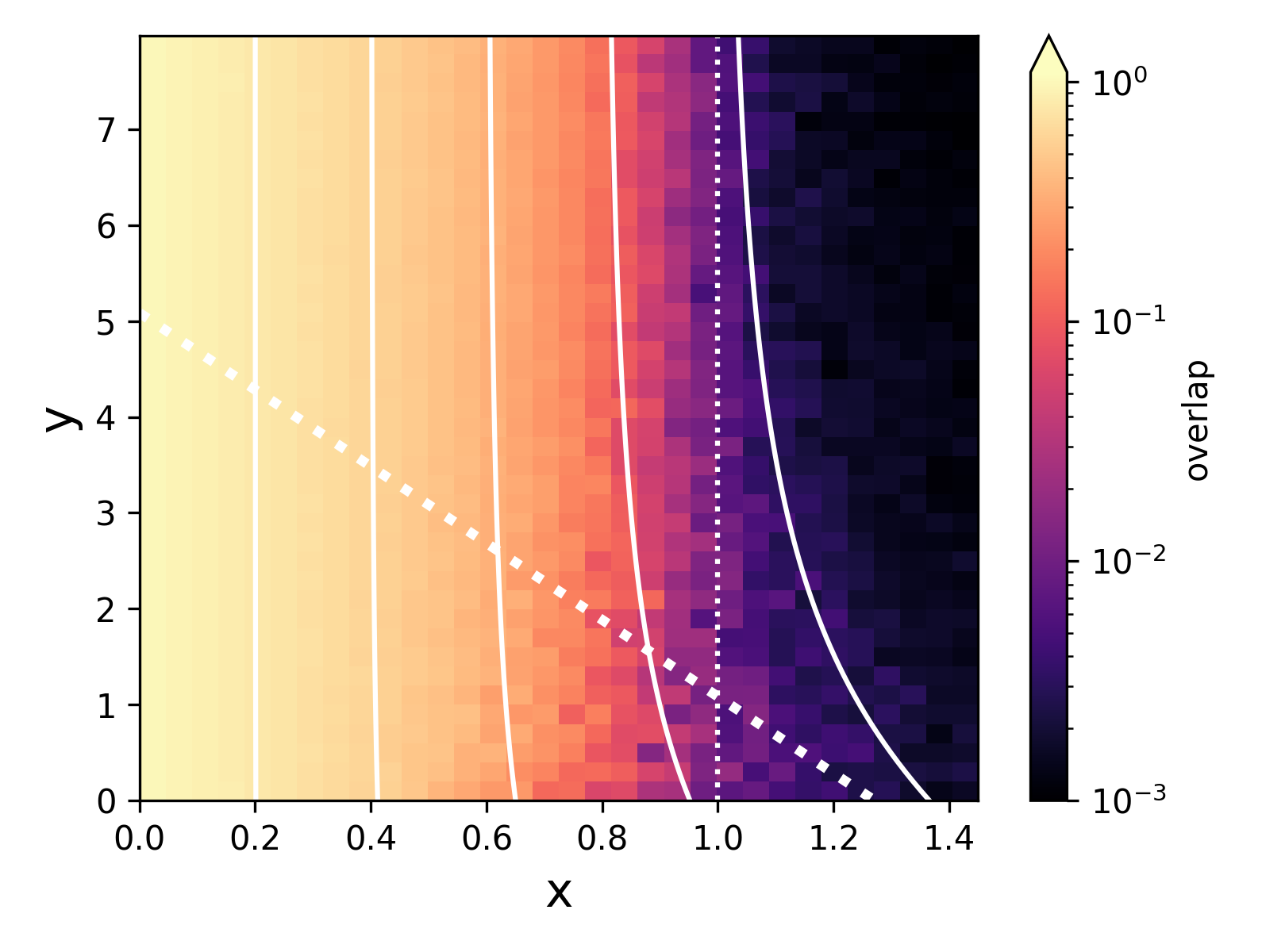
Figure 4: Phase diagram for genomes evolving under fitness (8) in the $(x=\mu/f,y=r/(2f))$ plane. The heatmap shows the Edwards–Anderson overlap $q$, see text and color bar, for a simulated population of $N=10^{4}$ individuals in the case of non-homogeneous recombination matrix $c_{ij}=\frac{1}{2}(1-\rho^{|i-j|})$ with $\rho=0.6$. The theoretical white lines were derived for recombination correlation $c_{ij}=\frac{1}{2}$, see main text. The critical line $x=2\tilde{\chi}^{st}(1)-2\chi^{st}(1)-1$ (rightmost solid curve) separates PM (right) and FM (left) phases, and approaches the $x=1$ line (thin dashed) when $y\gg 1$. Contour lines corresponding to $\chi_{FM}^{2}=0.2,.0.4,0.6,0.8$ (from right to left) are shown in the FM phase. The thick dashed line stands for $a=a_{c}\approx 2.542$, showing that $a>a_{c}$ throughout the PM phase.

VII Ferromagnetic phase

In the broken symmetry phase, hereafter referred to as ferromagnetic (FM), we expect the allele frequencies not to vanish any longer, and be equal to $\chi_{i}=\chi_{FM}$, up to a global reversal symmetry. Repeating the procedure followed in the PM phase we again consider the generating function $\tilde{\chi}^{st}(z)$ for the correlations $\chi^{st}(d)$ at distances $d\geq 1$. According to eqn. (4) the average allele frequency reads

$$\chi_{FM}^{2} = 1-x+2\sum_{d\geq 2}\chi^{st}(d)$$ (14)

$$= x-\big{[}2\tilde{\chi}^{st}(1)-2\chi^{st}(1)-1\big{]}\ ,$$

where the generating function of the correlations is now given by $\tilde{\chi}^{st}(z)=G\big{(}z,\chi_{FM}^{2}\big{)}$, see (10). As in the PM case, $\chi^{st}(1)$ is appropriately chosen to remove the spurious singularities inside the unit circle in the complex $z$–plane. By solving numerically the self-consistent eqns. (10) and (14) we were able to compute $\chi_{MF}^{2}$ throughout the ($x,y$) plane. As expected, $\chi_{MF}$ is non zero to the left of the border line of the region of stability of the PM phase; contour lines for $\chi_{FM}^{2}$ in the FM phase are shown in Fig. 4. Notice that, for a large range of parameter values, correlations decays very fast with distance as expected in the QLE phase, and $\chi_{FM}\simeq\sqrt{1-x}$ according to eqn. (14). In addition, we have numerically checked that condition (7) is met everywhere in the FM and PM phases, i.e. $2\sum_{d\geq 1}\chi^{st}(d)<1$.

VII.1 Short term dynamics: allele domains

Simulations show that, after a transient, the $\chi_{i}$’s reach apparently stationary values, with up and down domains of height $\pm\chi_{FM}$, see Fig. 5. Domains are of variable lengths, and are separated by characteristic domain walls.

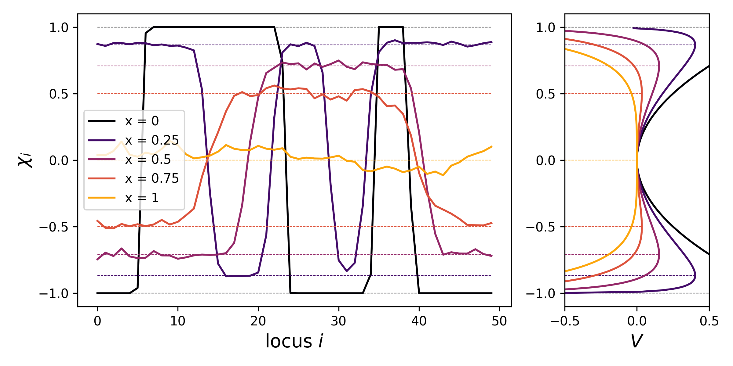
Figure 5: Left: Allele frequencies $\chi_{i}$ for one population evolved over 500 generations in the FM phase and for different values of the ratio $x$. Parameters: $f=0.028,N=10^{4},L=50,r=0.85$ and $c_{ij}=\frac{1}{2}(1-\rho^{|i-j|})$ with $\rho=0.6$. Dashed horizontal lines show $\pm\sqrt{1-x}$. Right: effective potential $V(\chi)$ for respective value of $x$ shown in the legend and horizontal lines locating the maxima of the potential in $\chi_{FM}=\pm\sqrt{1-x}$.

The shape of walls separating contiguous domains can be analytically characterized in the $r\to\infty$ limit. For $x$ close to 1 and $L\gg 1$, a smooth, continuum limit for the index $i\to z$ can be taken. In this approximation, we write $\chi_{i+1}+\chi_{i-1}-2\chi_{i}\simeq\chi^{\prime\prime}(z)$ in the stationary regime, and find, according to (4),

$$\chi^{\prime\prime}(z)=\frac{2\,x\,\chi(z)}{1-\chi^{2}(z)}-2\,\chi(z)\ ,$$ (15)

After integration, we obtain $\frac{1}{2}\,\chi^{\prime}(z)^{2}+V\big{(}\chi(z)\big{)}=E$, where $E$ is a constant and the potential is $V(\chi)=x\ln\left(1-\chi^{2}\right)+\chi^{2}$. Hence, finding the stationary profile of the spin average values is equivalent to a classical mechanics problem for a point-like particle of coordinate $\chi$ and unit mass, moving in the potential energy $V$ over fictitious time $z$. The potential $V(\chi)$ is symmetric in $0$, has two maxima in $\chi=\pm\chi_{FM}(x)$ and a local minimum in $\chi=0$ see Fig. 5(right). The trajectories $\chi(z)$ with conserved energy $E=V\big{(}\chi_{FM}\big{)}$ define the domain wall profiles. These profiles depend on the value of $x$, and are in good agreement with Fig. 5(left).

VII.2 Long-term dynamics: domain coarsening

On longer time scales, the domain walls described in Fig. 5 undergo a diffusive process, due to the noise resulting from finite (population) size sampling. Domain walls merge when they encounter, and the system will eventually settle into a final state with uniform frequency $\pm\chi_{FM}$. The characteristic time the system needs to converge into the uniformly magnetized state is shown in Fig. 6. It depends on the population size $N$ and on the genome length $L$, and is expected to scale as

$$\tau\sim\tau_{0}\times L^{2}\times N\ ,$$ (16)

where $\tau_{0}$ depends on the intensive parameters, such as the mutation/fitness ratio $x$. The scaling in (16) stems from the following simple argument. The typical size of domains grow with time as $\sim t^{1/2}$ according to the Allen-Cahn theory of coarsening for non-conserved fields Bray (1994). Hence a single domain will occupy the whole genome after a time given by $L^{2}/D$, where $D$ is the diffusion coefficient. Here, $D$ is expected to be inversely proportional to the population size $N$. This scaling is corroborated by the numerical results reported in Fig. 6.

Figure 6: FM phase: Nb. of generations required for convergence towards the uniform frequency state $\chi=\chi_{FM}$ vs. population size $N$ for different values of $x$. The dashed lines stand for the linear regression of the data. Each point is the average over 10 simulations. Parameters: $r=0.85$, $f=0.028$, $L=50$, $c_{i\neq j}=\frac{1}{2}$.

VIII Conclusions

We have here introduced a Gaussian closure scheme for the dynamics of multi-allele correlations across an infinite-size population of genomes evolving under recombination, mutation and selection. Informally speaking, the distribution of genomes at time $t$ is described as a cloud of covariance matrix $\chi_{ij}(t)$ around an ”average” genome (set of allele frequencies) $\chi_{i}(t)$. These 1- and 2-point correlations obey a set of $\frac{1}{2}L(L+1)$ coupled deterministic, non-linear first order differential equations, where $L$ is the genome length. For the sake of simplicity, we have assumed that alleles can be in one out of two possible states. While this assumption may already lead to quantitative behaviors similar to real systems Shekhar et al. (2013) it can be easily extended to multi-categorical (Potts) variables Gao et al. (2019).

Our scheme can be formally seen as a practical way to investigate the QLE regime beyond the large–$r$ perturbative approach initiated by Kimura Kimura (1965). While our eqns. (5) allow us to find back the QLE expressions for $\chi_{ij}$ at high recombination Zeng et al. (2020), they include contributions to all orders in powers of $1/r$ and can be exploited for generic recombination and mutation rates, as well as for any fitness function, and unveil non-trivial behaviors taking place at intermediate values of their defining parameters. An illustration is provided by the model analyzed in detail in this paper, in which two competing genomes, far away from each other in terms of allele composition have maximal and equal fitness. We find, at low enough mutation rate, a phase transition from a paramagnetic (PM) phase in which the distribution is broad and encompasses the two fittest genomes to a ferromagnetic (FM) regime, in which one of the genomes eventually dominates. We stress that, both in the PM and FM phases, correlations decay exponentially with the distance between the alleles along the genome, which is also their distance on the epistatic interaction graph. Hence, both phases formally belong to the QLE regime, even when $r$ is not large and $\mu$ is not small. However, contrary to a usual, informal definition of QLE, the genome distribution is not parametrized by the allele frequencies $\chi_{i}$ only, but also by the correlations $\chi_{ij}$, a consequence of the finiteness of $r$ and $\mu$.

Some aspects of the present work would deserve further investigation. First, while determining the range of validity of closure schemes is generally a complicated issue, e.g. in the case of small chemical systems Schnoerr et al. (2015), we have here derived some sufficient condition, see eqn. (7). This condition will break down if the genome distribution is multi-modal and correlations are not small, as is the case in the Clonal Competition (CC) regime Neher et al. (2013). However, even in CC, we may expect that our scheme remain adequate to describe locally the distribution of genomes attached to a clone. Therefore, it would be interesting to consider mixtures of Gaussian Ansätze, each describing a clone, an approximation which could be numerically tractable for sufficiently small numbers of clones and alleles.

Second, our approach offers, in principle, a practical way to infer the fitness determinants ($f_{i},f_{ij}$) from the statistics of sequence data. Approaches to interpret correlations are needed as epistatis is notoriously difficult to infer from observation of mean fitness alone McCandlish et al. (2015). Recently, the present Gaussian scheme was successfully used to reconstruct epistatic contributions from synthetic data Zeng et al. (2020). We hope the present approach will help put the inverse statistical approaches to protein sequence data Cocco et al. (2018) onto firm population genetics grounds.

Appendix A Derivation of dynamical equations for the first and second moments

Under the selection, mutation and recombination steps described in the main text the distribution of genomes at time $t$, $P({\bf s},t)$, obeys the Fokker-Planck-like equation:

$$\dot{P}({\bf s},t) = \big{(}F({\bf s})-\langle F\rangle\big{)}\,P({\bf s},t)+\mu\sum_{i=1}^{L}\big{(}P({\bf s}^{(i)},t)-P({\bf s},t)\big{)}$$

$$+ r \sum_{\bm{\xi},{\bf s}^{\prime}}C(\bm{\xi})\big{(}P({\bf s}^{m},t)P({\bf s}^{f},t)-P({\bf s},t)P({\bf s}^{\prime},t)\big{)},$$ (17)

which is identical to eqn (7) in Neher and Shraiman (2011). In the above equation, ${\bf s}^{(i)}$ denotes genome $\bf s$ in which allele $i$ has been flipped, $s_{i}\to-s_{i}$. By multiplying the above equation by $s_{i}$ or $s_{i}s_{j}$ and summing over all genomes $\bf s$ we obtain the evolution equations for the moments $\chi_{i}$ or $\chi_{ij}$, that is, $\dot{\chi}_{i}=\langle s_{i}\big{(}F({\bf s})-\langle F\rangle\big{)}\rangle-2\mu\chi_{i}$ and $\dot{\chi}_{ij}=\langle(s_{i}-\chi_{i})(s_{j}-\chi_{j})\big{(}F({\bf s})-\langle F\rangle\big{)}\rangle-(4\mu+rc_{ij})\chi_{ij}$, where the fitness function is defined in (2). The above equations coincide with eqns (8) and (10) in Neher and Shraiman (2011). We are left with the evaluation of the averages $\langle\cdot\rangle$ in the above equations. After replacement of quadratic terms $s_{k}^{2}$ with 1, the polynomial to be averaged is of degree zero or one in each variable $a_{k}=s_{k}-\chi_{k}$. We then forget about the discrete nature of the $a_{k}$’s, and take them as multivariate Gaussian variables with zero means and covariance matrix $\chi_{k\ell}$. Hence all odd moments vanish, and even moments can be computed from Wick’s theorem, e.g. $\langle a_{k}a_{\ell}a_{m}a_{n}\rangle=\chi_{k\ell}\chi_{mn}+\text{2\ other pairings}$. A systematic evaluation of all terms lead to (4) and (5).

Appendix B Contributions to $k^{th}$ moment

The approximation scheme describe in Appendix A can be used to compute moments of any order, such as $\chi_{i_{1},i_{2},...,i_{k}}=\langle\prod_{\alpha=1}^{k}(s_{i_{\alpha}}-\chi_{i_{\alpha}})\rangle$ with $k\geq 3$. In the stationary regime, we obtain

$$\chi_{i_{1},i_{2},...,i_{k}} = \frac{1}{G_{k}}\bigg{\langle}\bigg{\{}\prod_{\alpha=1}^{k}a_{i_{\alpha}}-\sum_{\alpha=1}^{k}(a_{i_{\alpha}}+\chi_{i_{\alpha}})\langle\prod_{\beta(\neq\alpha)}a_{i_{\beta}}\rangle\bigg{\}}$$ (18)

$$\times \big{(}\sum_{i}\hat{f}_{i}a_{i}+\sum_{i<j}f_{ij}(a_{i}a_{j}-\chi_{ij})\bigg{\rangle}$$

where $\hat{f}_{i}+\sum_{j(\neq i)}f_{ji}\chi_{j}$, $G_{k}=2k\mu+rc_{i_{1},i_{2},...,i_{k}}$, and $c_{i_{1},i_{2},...,i_{k}}$ is the probability (computed with $C(\bm{\xi})$) that all $k$ alleles do not come from the same parent (father or mother). Careful inspection of the polynomial in the $a_{k}$ variables (after replacements $a_{i}^{2}\to 1-\chi_{i}^{2}-2\chi_{i}a_{i}$ to enforce $s_{i}^{2}=1$) and of the effects of Wick’s contraction shows that terms appearing in the average $\langle\cdot\rangle$ above are of the form $M\times C\times(\chi_{ij})^{E}\times I$, where $\chi_{ij}$ stands for a generic 2-point moment, and (1) the exponent $E$ is equal to $\frac{\ell}{2}$, where $\ell$ is an integer comprised between $k-2$ and $k+2$, depending on the parity of $k$ and the term considered; (2) the combinatorial factor $C$ is equal to $(E-1)!!$; (3) the multiplicity $M$ is bounded by $L^{3}$; (4) the interaction term $I$ is a polynomial of degree $\leq 2$ in two of the $\chi_{i_{\alpha}}$’s ($\alpha=1...k$), and is proportional to one local fitness term $\hat{f}_{i}$ or epistatic coupling $f_{ij}$.

References

- Barton and de Vladar (2009) N. H. Barton and H. P. de Vladar, Genetics 181, 997 (2009).
- Kimura (1965) M. Kimura, Genetics 52, 875 (1965).
- Neher and Shraiman (2011) R. A. Neher and B. I. Shraiman, Reviews of Modern Physics 83, 1283 (2011).
- Neher and Leitner (2010) R. A. Neher and T. Leitner, PLoS Comput Biol 6, e1000660 (2010).
- Gao et al. (2019) C.-Y. Gao, F. Cecconi, A. Vulpiani, H.-J. Zhou, and E. Aurell, Physical biology 16, 026002 (2019).
- Cocco et al. (2018) S. Cocco, C. Feinauer, M. Figliuzzi, R. Monasson, and M. Weigt, Reports on Progress in Physics 81, 032601 (2018).
- Turelli and Barton (1994) M. Turelli and N. H. Barton, Genetics 138, 913 (1994).
- Bürger (2000) R. Bürger, The mathematical theory of selection, recombination, and mutation (John Wiley & Sons, 2000).
- Jain and Stephan (2017) K. Jain and W. Stephan, Molecular biology and evolution 34, 3169 (2017).
- Barghi et al. (2020) N. Barghi, J. Hermisson, and C. Schlötterer, Nature Reviews Genetics , 1 (2020).
- Flajolet and Sedgewick (2009) P. Flajolet and R. Sedgewick, Analytic combinatorics (cambridge University press, 2009).
- Bray (1994) A. Bray, Adv. Phys. (1994).
- Shekhar et al. (2013) K. Shekhar, C. F. Ruberman, A. L. Ferguson, J. P. Barton, M. Kardar, and A. K. Chakraborty, Physical review E 88, 062705 (2013).
- Zeng et al. (2020) H.-L. Zeng, E. Mauri, V. Dichio, S. Cocco, R. Monasson, and E. Aurell, arXiv preprint arXiv:2006.16735 (2020).
- Schnoerr et al. (2015) D. Schnoerr, G. Sanguinetti, and R. Grima, The Journal of Chemical Physics 143, 11B610_1 (2015).
- Neher et al. (2013) R. A. Neher, M. Vucelja, M. Mezard, and B. I. Shraiman, Journal of Statistical Mechanics: Theory and Experiment 2013, P01008 (2013).
- McCandlish et al. (2015) D. M. McCandlish, J. Otwinowski, and J. B. Plotkin, Evolution 69, 2359 (2015).