Galilean-Invariant XEFT
at Next-to-Leading Order

Abstract

XEFT is a low-energy effective field theory for charm mesons and pions that provides a systematically improvable description of the $X(3872)$ resonance. To simplify calculations beyond leading order, we introduce a new formulation of XEFT with a dynamical field for a pair of charm mesons in the resonant channel. We simplify the renormalization of XEFT by introducing a new renormalization scheme that involves the subtraction of amplitudes at the complex $D^{*0}\bar{D}^{0}$ threshold. The new formulation and the new renormalization scheme are illustrated by calculating the complex pole energy of $X$ and the $D^{*0}\bar{D}^{0}$ scattering amplitude to next-to-leading order using Galilean-invariant XEFT.

I Introduction

The $X(3872)$ was the first of the dozens of exotic hadrons whose fundamental constituents include a heavy quark and its antiquark that have been discovered since the beginning of the century Ali:2017jda ; Olsen:2017bmm ; Karliner:2017qhf ; Brambilla:2019esw . Determining the nature of $X$ remains central to the problem of understanding the exotic heavy hadrons. The discovery of $X$ by the Belle collaboration in 2003 was through the decay mode $J/\psi\,\pi^{+}\pi^{-}$, which reveals that its constituents include a charm quark and its antiquark ($c\bar{c}$) Choi:2003ue . The $J^{PC}$ quantum numbers of $X$ were determined to be $1^{++}$ by the LHCb collaboration in 2013 Aaij:2013zoa . The possibilities for the particle structure of $X$ that are compatible with this information include

• the $\chi_{c1}(2P)$ charmonium state, whose quark constituents are $c\bar{c}$,

• a compact isospin-1 tetraquark meson, whose diquark constituents are $(cu)(\bar{c}\bar{u})-(cd)(\bar{c}\bar{d})$,

• an isospin-0 charm-meson molecule, whose hadron constituents are $(D^{*0}\bar{D}^{0}+D^{0}\bar{D}^{*0})+(D^{*+}D^{-}+D^{+}D^{*-})$, which correspond to quark constituents $(c\bar{u})(\bar{c}u)+(c\bar{d})(\bar{c}d)$.

The Belle collaboration discovered $X$ at a mass that was surprisingly close to the scattering threshold for $D^{*0}\bar{D}^{0}$. The measured energy relative to the threshold was $(+0.9\pm 1.3)$ MeV Choi:2003ue . They put an upper bound on its width of about 2.3 MeV. Over the subsequent years, the measurements of the masses of $X$, $D^{*0}$, and $\bar{D}^{0}$ have all been improved significantly. The LHCb collaboration has recently made the most precise measurements of the mass of $X$ to date, and they made the first measurements of its width Aaij:2020qga ; Aaij:2020xjx . With the line shape of the $X$ in the $J/\psi\,\pi^{+}\pi^{-}$ decay channel modeled by that of a Breit-Wigner resonance, their results for the energy relative to the $D^{*0}\bar{D}^{0}$ threshold and for the width are

$$E_{\mathrm{BW}} = (-0.07\pm 0.12)~{}\mathrm{MeV},$$ (1a)

$$\Gamma_{\mathrm{BW}} = (1.19\pm 0.19)~{}\mathrm{MeV}.$$ (1b)

An alternative prescription for the energy and the width of a resonance are the real and imaginary parts of the pole energy $E_{X}-i\Gamma_{X}/2$. With the line shape modeled by that of a Flatté amplitude that takes into account the width of the $D^{*0}$, the LHCb collaboration obtained $(+0.025-0.140\,i)$ MeV for the pole energy relative to the $D^{*0}\bar{D}^{0}$ threshold Aaij:2020qga . The energy $E_{X}$ is consistent with the measurement in Eq. (1a), while the width $\Gamma_{X}$ is about 4 times smaller than the measurement in Eq. (1b).

The extremely small energy of $X$ relative to the $D^{*0}\bar{D}^{0}$ threshold in Eq. (1a) has dramatic implications for the structure of $X$. The quantum numbers $1^{++}$ of $X$ imply that it has an S-wave coupling to $D^{*0}\bar{D}^{0}$ and $D^{0}\bar{D}^{*0}$. Since these mesons are electrically neutral, they interact with each other through short-range interactions with a range of order $1/m_{\pi}$, where $m_{\pi}$ is the pion mass. However the tiny energy of $X$ relative to the $D^{*0}\bar{D}^{0}$ threshold implies that the interaction between the charm mesons is resonant. Thus $X$ is an S-wave resonance near the threshold for a pair of particles with short-range interactions. General principles of quantum mechanics guarantee that $X$ must have universal properties determined by its binding energy Braaten:2003he . They guarantee that the dominant component of $X$ must be a charm-meson molecule with the particle structure

$$X=\frac{1}{\sqrt{2}}\big{(}D^{*0}\bar{D}^{0}+D^{0}\bar{D}^{*0}\big{)}.$$ (2)

If $E_{X}<0$, $X$ is a bound state whose spatial structure is described by a universal wavefunction $\exp(-r/a)/r$, where $a=1/\sqrt{2\mu|E_{X}|}$ is the S-wave scattering length of $D^{*0}\bar{D}^{0}$ in the $C=+$ channel and $\mu$ is the reduced mass of $D^{*0}\bar{D}^{0}$. The mean separation of the constituents is $\langle r\rangle=a/2$. If the energy $E_{X}$ is identified with the Breit-Wigner energy in Eq. (1a), the lower bound on the energy at the 90% confidence level is $E_{X}>-0.22$ MeV. Thus the mean separation is larger than 4.8 fm.

The universality of S-wave near-threshold resonances is a truly remarkable aspect of quantum mechanics Braaten:2004rn . If a model for the $X$ with any particle structure, such as one of those itemized above, is extended to allow couplings to $D^{*0}\bar{D}^{0}$ and $D^{0}\bar{D}^{*0}$ scattering states, it will be dramatically transformed by the resonant couplings to the scattering states. If the model has an adjustable parameter that can be used to tune the resonance energy to the $D^{*0}\bar{D}^{0}$ threshold, the resonance will in the limit develop the particle structure in Eq. (2) with the universal wavefunction $\exp(-r/a)/r$. This remarkable phenomenon is widely recognized in the case of a charm-meson molecule. That it occurs also in the case of a charmonium state or a compact tetraquark is not as widely recognized.

The universality of S-wave near-threshold resonances provides a basis for a systematically improvable treatment of the $X$ resonance using effective field theory. An appropriate effective field theory was invented by Fleming et al. and named XEFT Fleming:2007rp . XEFT is a nonrelativistic effective field theory for charm mesons and pions. In the simplest version of XEFT, the only fields are those for the neutral charm mesons $D^{*0}$, $\bar{D}^{*0}$, $D^{0}$, and $\bar{D}^{0}$ and the neutral pion $\pi^{0}$. The only components of $X$ that are treated explicitly are those in Eq. (2) and $D^{0}\bar{D}^{0}\pi^{0}$. The effects of all other particles must be taken into account in the parameters of XEFT. In particular, different models for $X$ with resonance energy far enough away from the $D^{*0}\bar{D}^{0}$ threshold, such as those itemized above, correspond to different choices for the parameters of XEFT. The simplest version of XEFT is sufficient if the total energy of $D^{*0}\bar{D}^{0}$, $D^{0}\bar{D}^{*0}$, or $D^{0}\bar{D}^{0}\pi^{0}$ is close enough to the $D^{*0}\bar{D}^{0}$ threshold. The region of validity of XEFT can be extended by adding fields for the charged charm mesons $D^{*+}$, $D^{*-}$, $D^{+}$, and $D^{-}$ and the charged pions $\pi^{+}$ and $\pi^{-}$. In this case, the additional components of $X$ that are treated explicitly are $D^{*+}D^{-}$, $D^{+}D^{*-}$, $D^{+}D^{-}\pi^{0}$, $D^{+}\bar{D}^{0}\pi^{-}$, and $D^{0}D^{-}\pi^{+}$.

An effective field theory can be simplified by taking advantage of exact and approximate symmetries. A remarkable aspect of the sector of QCD consisting of $D^{*}\bar{D}$, $D\bar{D}^{*}$, and $D\bar{D}\pi$ that is described by XEFT is that the sum of the masses is very nearly conserved. Galilean invariance is a possible symmetry of a nonrelativistic field theory that requires exact conservation of the kinetic mass. In Ref. Braaten:2015tga , a Galilean formulation of XEFT was developed. Galilean invariance provides strong constraints on the ultraviolet (UV) divergences from loop amplitudes. It therefore greatly simplifies the renormalization of XEFT. In this paper, we introduce a new formulation of Galilean-invariant XEFT with a dynamical field for a pair of charm mesons in the resonant channel. This new formulation further simplifies calculations beyond leading order.

The accuracy of an effective field theory can be greatly improved by using an appropriate renormalization scheme. Analytic results can also be greatly simplified by the choice of an appropriate renormalization scheme. In the pioneering paper on XEFT, the momentum distribution for the decay of $X$ into $D^{0}\bar{D}^{0}\pi^{0}$ was calculated at next-to-leading order (NLO) using dimensional regularization with power divergence subtraction Fleming:2007rp . The only UV divergences are linear divergences, and they were removed by absorbing them into interaction parameters. In Ref. Braaten:2015tga , the elastic scattering amplitude for $D^{*0}\bar{D}^{0}$ was calculated at NLO using dimensional regularization in Galilean-invariant XEFT. There are both linear and logarithmic UV divergences, and they were removed by subtractions at the complex pole energy of $X$. In this paper, we introduce a simpler renormalization scheme for XEFT in which divergences are removed instead by subtractions at the complex threshold energy of $D^{*0}\bar{D}^{0}$. This new renormalization scheme greatly simplifies analytic results at NLO.

In Section II, we introduce Galilean invariance and we describe various formulations of XEFT. In Section III, we present the Lagrangian for the new formulation of Galilean-invariant XEFT with a dynamical pair field. In Section IV, we present the Feynman rules for this new formulation of XEFT. In Section V, we calculate the pair propagator at NLO and we obtain the complex pole energy of $X$ at NLO. In Section VI, we calculate the $D^{*0}\bar{D}^{0}$ elastic scattering amplitude at NLO and we analyze the breakdown of the effective range expansion from pion exchange. We summarize our results and suggest other useful applications in Section VII. In Appendix A, we present results for loop integrals that arise in calculations at NLO. In Appendix B, we present the results for individual Feynman diagrams for the $D^{*0}\bar{D}^{0}$ transition amplitude at NLO.

II Galilean-invariant XEFT

In this section, we introduce Galilean invariance, describe various formulations of XEFT, and give the numerical values of some of its parameters.

II.1 Galilean invariance

Galilean invariance is a possible space-time symmetry of a nonrelativistic field theory Hagen:1972pd ; Rosen:1972sh . In a nonrelativistic theory, the energy-momentum relation for an on-shell particle with rest energy $\varepsilon$ and kinetic mass $m$ is

$$E(p)=\varepsilon+p^{2}/(2m).$$ (3)

Galilean symmetry requires invariance under a Galilean boost with an arbitrary velocity vector $\bm{v}$. The effects of the Galilean boost on the energy and momentum are

$$E \longrightarrow E+\bm{v}\cdot\bm{p}+\frac{1}{2}mv^{2},$$ (4a)

$$\bm{p} \longrightarrow \bm{p}+m\bm{v}.$$ (4b)

The invariant energy $E-p^{2}/2m$ is invariant under Galilean boosts.

A unique feature of the sector of QCD consisting of spin-0 charm mesons $D$ and $\bar{D}$, spin-1 charm mesons $D^{*}$ and $\bar{D}^{*}$, and pions $\pi$ is that mass is very nearly conserved by the transitions $D^{*}\leftrightarrow D\pi$. In the decay $D^{*0}\to D^{0}\pi^{0}$, the sum of the masses of the $D^{0}$ and $\pi^{0}$ is lower than the mass of the $D^{*0}$ by 7.0 MeV, which is only 0.35%. Since the isospin splittings between the charm mesons are at most 4.8 MeV and the isospin splitting between $\pi^{+}$ and $\pi^{0}$ is 4.6 MeV, all the transitions $D^{*}\leftrightarrow D\pi$ come very close to satisfying mass conservation. There are no other hadrons with such narrow widths that have transitions that come so close to satisfying mass conservation.

Galilean invariance requires the exact conservation of the kinetic mass Hagen:1972pd . In a Galilean-invariant description of charm mesons and pions, the spin-0 charm mesons must all have the same kinetic mass $M$ and the pions must all have the same kinetic mass $m$. Conservation of kinetic mass then requires the kinetic mass of all the spin-1 charm mesons to be $M+m$.

In a nonrelativistic effective field theory for charm mesons, one can impose a phase symmetry that guarantees the separate conservation of the number $N_{c}$ of charm quarks and the number $N_{\bar{c}}$ of charm antiquarks. These quark numbers can be expressed in terms of meson numbers. In a theory with only neutral charm mesons and $\pi^{0}$, the quark numbers are

$$N_{c} = N_{D^{*0}}+N_{D^{0}},$$ (5a)

$$N_{\bar{c}} = N_{\bar{D}^{*0}}+N_{\bar{D}^{0}}.$$ (5b)

If the theory also includes charged charm mesons and charged pions, the charm quark number $N_{c}$ also includes the numbers of $D^{*+}$ and $D^{+}$. In a Galilean-invariant effective field theory for charm mesons and pions, the exact conservation of kinetic mass in the transitions $D^{*}\leftrightarrow D\pi$ provides motivation for introducing an additional phase symmetry that guarantees the conservation of pion number. In a theory with only neutral charm mesons and $\pi^{0}$, the pion number is

$$N_{\pi}=N_{\pi^{0}}+N_{D^{*0}}+N_{\bar{D}^{*0}}.$$ (6)

If the theory also includes charged charm mesons and charged pions, the pion number $N_{\pi}$ also includes the numbers of $\pi^{+}$, $\pi^{-}$, $D^{*+}$, and $D^{*-}$.

II.2 XEFT

XEFT is a nonrelativistic effective field theory for charm mesons and pions invented by Fleming et al. Fleming:2007rp . It provides a systematically improvable description of the sector of QCD consisting of $D^{*}\bar{D}$, $D\bar{D}^{*}$, and $D\bar{D}\pi$ with total energy near the $D^{*}\bar{D}$ threshold. It therefore can be used to calculate some properties of the $X$ resonance systematically. In XEFT with only neutral charm mesons and $\pi^{0}$, the only fields are complex scalar fields for $D^{0}$, $\bar{D}^{0}$, and $\pi^{0}$ and complex vector fields for $D^{*0}$ and $\bar{D}^{*0}$. For the sector of QCD consisting of $D^{*0}\bar{D}^{0}$, $D^{0}\bar{D}^{*0}$, $D^{0}\bar{D}^{0}\pi^{0}$, and $X$, the region of validity of XEFT with only neutral particles extends at most to the $D^{*+}D^{-}$ threshold, which is 8.2 MeV above the $D^{*0}\bar{D}^{0}$ threshold. The region of validity can be extended to higher energies by introducing additional fields for the charged charm mesons and the charged pions.

At leading order (LO) in the power counting of XEFT, the only adjustable parameter is the LO binding momentum $\gamma$ of $X$, which was assumed to be a real parameter in Ref. Fleming:2007rp . At next-to-leading order (NLO), there are additional adjustable interaction parameters. In Ref. Fleming:2007rp , XEFT was used to calculate the differential decay rate of $X$ into $D^{0}\bar{D}^{0}\pi^{0}$ at NLO. It depends on two additional adjustable real parameters: a length $r_{0}$ associated with the effective range in the resonant S-wave even-charge-conjugation ($C=+$) channel and a parameter for the coupling of $D^{*0}\bar{D}^{0}$ to $D^{0}\bar{D}^{0}\pi^{0}$. Fleming et al. calculated the partial decay rate of $X$ into $D^{0}\bar{D}^{0}\pi^{0}$ numerically as a function of the LO binding energy $\gamma^{2}/(2\mu)$. Their estimate of the width of the error band from the two NLO interaction parameters decreased from about 25% to about 10% as $\gamma^{2}/(2\mu)$ decreased from 0.1 MeV to 0.01 MeV. The relatively wide error bands even for extremely tiny values of $\gamma$ raises the question of whether the power-counting expansion for XEFT converges fast enough for it to be quantitatively useful. The original formulation of XEFT in Ref. Fleming:2007rp has also been applied to the $D^{*0}\bar{D}^{0}$ scattering length at NLO Jansen:2013cba . The NLO calculation of the decay rate for $X$ into $D^{0}\bar{D}^{0}\pi^{0}$ was recently revisited by Dai et al. Dai:2019hrf . They pointed out that the power-counting rules of chiral effective field theories for heavy mesons implied that there are two additional NLO interactions parameters: the S-wave scattering lengths for $D^{0}\bar{D}^{0}$ and for $D^{0}\pi^{0}$. Their estimate of the width of the error band from the four NLO interaction parameters decreased from about 60% to about 30% as $\gamma^{2}/(2\mu)$ decreased from 0.1 MeV to 0.01 MeV. The wide error bands even for extremely tiny values of $\gamma$ further emphasizes the convergence problem of XEFT.

An alternative formulation of XEFT was developed in Ref. Braaten:2015tga . It differs from the original formulation in Ref. Fleming:2007rp in three important ways:

1. Galilean invariance.

2. Systematic treatment of the width of $D^{*0}$, which requires the LO binding momentum $\gamma$ to be complex.

3. Complex on-shell (COS) renormalization scheme, in which the UV divergences in $D^{*0}\bar{D}^{0}$ and $D^{0}\bar{D}^{*0}$ amplitudes are removed by subtractions at the complex pole energy $E_{X}-i\Gamma_{X}/2$.

Taking into account the $D^{*0}$ width is essential if XEFT is to give an accurate description of the $X$ resonance. In the COS scheme, the adjustable real parameters at LO are $E_{X}$ and $\Gamma_{X}$. In Ref. Braaten:2015tga , Galilean-invariant XEFT was used to calculate the $D^{*0}\bar{D}^{0}$ scattering length at NLO. The result depends on a single additional adjustable parameter that can be identified with the parameter $r_{0}$ in Ref. Fleming:2007rp . One drawback of the COS scheme is that the analytic expression for the $D^{*0}\bar{D}^{0}$ scattering amplitude is rather complicated. Galilean invariance simplifies the renormalization of XEFT. It implies, for example, that the S-wave scattering lengths for $D^{0}\bar{D}^{0}$ and for $D^{0}\pi^{0}$, which were argued to be NLO parameters of XEFT in Ref. Dai:2019hrf , are not required by renormalization.

In this paper, we present an alternative formulation of Galilean-invariant XEFT. It differs from the formulation of Galilean-invariant XEFT in Ref. Braaten:2015tga in three important ways:

1. An additional complex vector field, which we call the pair field, that annihilates a pair of charm mesons in the resonant channel.

2. New Feynman rules in which $D^{*0}\bar{D}^{0}$ and $D^{0}\bar{D}^{*0}$ couple to the resonant channel only through the intermediate pair propagator.

3. Complex threshold (CT) renormalization scheme, in which the UV divergences in $D^{*0}\bar{D}^{0}$ and $D^{0}\bar{D}^{*0}$ amplitudes are removed by subtractions at the complex threshold for $D^{*0}\bar{D}^{0}$ scattering states.

The new Feynman rules simplify calculations beyond LO by making some cancellations of UV divergences between diagrams automatic. The CT scheme dramatically simplifies analytic expressions for amplitudes beyond LO. It reveals the existence of an additional adjustable interaction parameter at NLO that was not recognized in Ref. Braaten:2015tga . It may also provide a solution to the problem of the large NLO corrections in XEFT that were encountered in Refs. Fleming:2007rp ; Dai:2019hrf .

II.3 Known parameters

We denote the masses of $D^{*0}$, $D^{0}$, and $\pi^{0}$ by $M_{*0}$, $M_{0}$, and $m_{0}$, respectively. The difference between the $D^{*0}$ mass and the $D^{0}\pi^{0}$ threshold is

$$\delta\equiv M_{*0}-(M_{0}+m_{0})=(7.04\pm 0.03)~{}\mathrm{MeV}.$$ (7)

The decay width of the $D^{*0}$ can be predicted by assuming the decays $D^{*}\to D\pi$ respect chiral symmetry, isospin symmetry, and Lorentz invariance. The measured branching fraction for $D^{*0}\to D^{0}\pi^{0}$ is $B_{*0\pi}=(64.7\pm 0.9)\%$. Using the decay width of the $D^{*+}$ and the branching fractions for $D^{*0}\to D^{0}\pi^{0}$ and $D^{*+}\to D^{0}\pi^{+}$ as inputs, the prediction for the total $D^{*0}$ width is

$$\Gamma_{*0}\equiv\Gamma[D^{*0}]=(55.4\pm 1.5)~{}\mathrm{keV}.$$ (8)

In Galilean-invariant XEFT, the spin-0 charm mesons all have the same kinetic mass $M$ and the pions all have the same kinetic mass $m$. We choose the kinetic masses $M$ and $m$ of $D^{0}$ and $\pi^{0}$ to be equal to their physical masses $M_{0}$ and $m_{0}$, respectively. The rest energies of $D^{0}$ and $\pi^{0}$ are therefore both zero. Galilean invariance requires the kinetic mass of $D^{*0}$ to be $M+m$. The $D^{*0}$ has the complex rest energy

$$E_{*}=\delta-i\Gamma_{*0}/2,$$ (9)

where $\delta$ is the energy in Eq. (7) and $\Gamma_{*0}$ is the $D^{*0}$ width in Eq. (8).

The reduced mass $\mu_{\pi}$ for $D^{0}\pi^{0}$ and the reduced kinetic mass $\mu$ for $D^{*0}\bar{D}^{0}$ are

$$\mu_{\pi} \equiv \frac{mM}{M+m}=125.87~{}{\rm MeV},$$ (10a)

$$\mu \equiv \frac{M(M+m)}{2M+m}=965.0~{}{\rm MeV}.$$ (10b)

The ratio of these reduced masses is a small parameter in Galilean-invariant XEFT:

$$r\equiv\mu_{\pi}/\mu=0.1304.$$ (11)

The $D^{*0}$-to-$D^{0}\pi^{0}$ coupling constant in XEFT is conventionally denoted by $g/(2\sqrt{m}f_{\pi})$. This coupling constant can be determined from the partial width of $D^{*0}$ into $D^{0}\pi^{0}$:

$$\Gamma_{*0,\pi}\equiv\Gamma[D^{*0}\to D^{0}\pi^{0}]=\left(\frac{g^{2}}{4mf_{\pi}^{2}}\right)\frac{\mu_{\pi}}{3\pi}(2\mu_{\pi}\delta)^{3/2},$$ (12)

where $\delta$ is the energy in Eq. (7). It is convenient to define a coupling constant $g_{\pi}^{2}$ with dimensions 1/(momentum):

$$g_{\pi}^{2}\equiv(g^{2}/4mf_{\pi}^{2})\mu^{2}=\big{[}(29.7\pm 0.7)~{}\mathrm{MeV}\big{]}^{-1}.$$ (13)

III Lagrangian

In this section, we write down the Lagrangian for Galilean-invariant XEFT for the neutral charm mesons and $\pi^{0}$. We introduce a new form for the Lagrangian with a dynamical pair field for a pair of charm mesons in the resonant channel. We include all terms required to calculate to NLO in the XEFT power counting.

III.1 LO Lagrangian

The fields for the $D^{0}$ and $\bar{D}^{0}$ are complex scalar fields $D$ and $\bar{D}$. The field for the $\pi^{0}$ is a complex scalar field $\pi$. The fields for the $D^{*0}$ and $\bar{D}^{*0}$ are complex vector fields $\bm{D}$ and $\bar{\bm{D}}$. The kinetic terms in the Lagrangian for $D^{0}$ and $\pi^{0}$ are

$${\cal L}_{D} = D^{\dagger}\left[i\partial_{t}+\nabla^{2}/(2M)\right]D,$$ (14a)

$${\cal L}_{\pi} = \pi^{\dagger}\left[i\partial_{t}+\nabla^{2}/(2m)\right]\pi.$$ (14b)

The kinetic term for $\bar{D}^{0}$ is obtained from Eq. (14a) by replacing $D$ by $\bar{D}$. The kinetic term in the Lagrangian for $D^{*0}$ is

$${\cal L}_{D^{*}}=\bm{D}^{\dagger}\cdot\left[i\partial_{t}+\nabla^{2}/(2(M+m))-E_{*}\right]\bm{D},$$ (15)

where $E_{*}$ is the complex rest energy of $D^{*0}$ in Eq. (9). The kinetic term for $\bar{D}^{*0}$ is obtained by replacing $\bm{D}$ by $\bar{\bm{D}}$.

There is a resonance in the S-wave channel for the superposition of $D^{*0}\bar{D}^{0}$ and $D^{0}\bar{D}^{*0}$ with even charge conjugation ($C=+$) in Eq. (2). The interaction term in the Lagrangian for XEFT at LO is a contact interaction in the resonant channel:

$${\cal L}_{\mathrm{LO,int}}=-\frac{C_{0}}{2}\,\left(\bar{D}\bm{D}+D\bar{\bm{D}}\right)^{\dagger}\cdot\left(\bar{D}\bm{D}+D\bar{\bm{D}}\right).$$ (16)

It is convenient to introduce a complex vector field $\bm{\phi}$ that we call the pair field that annihilates a pair of charm mesons in the resonant channel:

$$\bm{\phi}=\frac{C_{0}}{\sqrt{2}}\,\left(\bar{D}\bm{D}+D\bar{\bm{D}}\right).$$ (17)

The normalization factor has been chosen for later convenience. Using the pair field $\bm{\phi}$, we can write down an alternative interaction term in the Lagrangian for XEFT at LO:

$${\cal L}_{\mathrm{LO,int}}=\frac{1}{C_{0}}\,\bm{\phi}^{\dagger}\cdot\bm{\phi}-\frac{1}{\sqrt{2}}\left[\left(\bar{D}\bm{D}+D\bar{\bm{D}}\right)^{\dagger}\cdot\bm{\phi}+\bm{\phi}^{\dagger}\cdot\left(\bar{D}\bm{D}+D\bar{\bm{D}}\right)\right].$$ (18)

The field equation for $\bm{\phi}$ implies Eq. (17). The field equation can be used to eliminate $\bm{\phi}$ from Eq. (18), which reduces it to Eq. (16). The two interaction Lagrangians are therefore equivalent.

III.2 NLO interaction terms

In the original paper on XEFT in Ref. Fleming:2007rp , all the interaction terms in the Lagrangian needed for calculations to next-to-leading order (NLO) in the power-counting of XEFT were written down explicitly. They included pion interaction terms that allow transitions between $D^{*0}$ and $D^{0}\pi^{0}$ and between $\bar{D}^{*0}$ and $\bar{D}^{0}\pi^{0}$. In Galilean-invariant XEFT, the pion interaction terms are Braaten:2015tga

$${\cal L}_{D^{*}\leftrightarrow D\pi}=\frac{g}{2\sqrt{m}f_{\pi}}\left[\bm{D}^{\dagger}\cdot\big{(}D\overleftrightarrow{\bm{\nabla}}\pi\big{)}+\big{(}D\overleftrightarrow{\bm{\nabla}}\pi\big{)}^{\dagger}\cdot\bm{D}+\bar{\bm{D}}^{\dagger}\cdot\big{(}\bar{D}\overleftrightarrow{\bm{\nabla}}\pi\big{)}+\big{(}\bar{D}\overleftrightarrow{\bm{\nabla}}\pi\big{)}^{\dagger}\cdot\bar{\bm{D}}\right],$$ (19)

where $\overleftrightarrow{\bm{\nabla}}=(M\overrightarrow{\bm{\nabla}}-m\overleftarrow{\bm{\nabla}})/(M+m)$ is a Galilean-invariant derivative. The pion interaction term in the Lagrangian for original XEFT in Ref. Fleming:2007rp can be obtained by replacing the operator $\overleftrightarrow{\bm{\nabla}}$ in Eq. (19) by $\overrightarrow{\bm{\nabla}}$.

The NLO interaction terms in the Lagrangian for original XEFT in Ref. Fleming:2007rp include $\nabla^{2}$ interaction terms that produce transitions between incoming $D^{*0}\bar{D}^{0}$ or $D^{0}\bar{D}^{*0}$ and outgoing $D^{*0}\bar{D}^{0}$ or $D^{0}\bar{D}^{*0}$. There are equivalent interaction terms involving the pair field $\bm{\phi}$. In Galilean-invariant XEFT, the $\nabla^{2}$ interaction terms involving $\bm{\phi}$ are

$${\cal L}_{\nabla^{2}} = \frac{C_{2}}{2\sqrt{2}\,C_{0}}\left[\bm{\phi}^{\dagger}\cdot\Big{(}\bar{D}\overleftrightarrow{\bm{\nabla}}^{2}\bm{D}+D\overleftrightarrow{\bm{\nabla}}^{2}\bar{\bm{D}}\Big{)}+\Big{(}\bar{D}\overleftrightarrow{\bm{\nabla}}^{2}\bm{D}+D\overleftrightarrow{\bm{\nabla}}^{2}\bar{\bm{D}}\Big{)}^{\dagger}\cdot\bm{\phi}\right],$$ (20)

where $\overleftrightarrow{\bm{\nabla}}=(M\overrightarrow{\bm{\nabla}}-(M+m)\overleftarrow{\bm{\nabla}})/(2M+m)$ is a Galilean-invariant derivative. The $\nabla^{2}$ interaction terms in Ref. Braaten:2015tga can be obtained by eliminating $\bm{\phi}$ using the field equation in Eq. (17). The $\nabla^{2}$ interaction terms in the Lagrangian for original XEFT in Ref. Fleming:2007rp can be obtained by replacing the operator $\overleftrightarrow{\bm{\nabla}}$ in Eq. (20) by $(\overrightarrow{\bm{\nabla}}-\overleftarrow{\bm{\nabla}})/2$ and then eliminating $\bm{\phi}$ using its field equation.

The NLO interaction terms in the Lagrangian for original XEFT in Ref. Fleming:2007rp include counterterms that produce transitions between incoming $D^{*0}\bar{D}^{0}$ or $D^{0}\bar{D}^{*0}$ and outgoing $D^{*0}\bar{D}^{0}$ or $D^{0}\bar{D}^{*0}$. There is an equivalent counterterm involving the pair field only:

$${\cal L}_{\mathrm{counter}}=-(1/C_{0}^{2})\big{[}\delta C_{0}\,\bm{\phi}^{\dagger}\cdot\bm{\phi}+D_{0}\,\bm{\phi}^{\dagger}\cdot(iD_{t}-E_{*})\bm{\phi}\big{]}.$$ (21)

where $iD_{t}=i\partial_{t}+\nabla^{2}/(2(2M+m))$ is a Galilean-invariant derivative. The constant subtracted from $iD_{t}$ is arbitrary. The choice $E_{*}$ corresponds to the complex on-shell renormalization scheme for the $D^{*0}$ propagator. The NLO counterterms in the Lagrangian for original XEFT in Ref. Fleming:2007rp can be obtained by eliminating $\bm{\phi}$ from Eq. (21) using the field equation in Eq. (17).

In the original paper on XEFT in Ref. Fleming:2007rp , the Lagrangian included another NLO interaction term that allowed transitions between $D^{*0}\bar{D}^{0}$ or $D^{0}\bar{D}^{*0}$ and $D^{0}\bar{D}^{0}\pi^{0}$. There is an equivalent NLO interaction term involving the pair field. In Galilean-invariant XEFT, the $D\bar{D}\pi$ interaction terms involving $\bm{\phi}$ are

$${\cal L}_{D\bar{D}\pi}=\frac{B_{1}}{\sqrt{2m}\,C_{0}}\left[\bm{\phi}^{\dagger}\cdot\big{(}D\bar{D}\overleftrightarrow{\bm{\nabla}}\pi\big{)}+\big{(}D\bar{D}\overleftrightarrow{\bm{\nabla}}\pi\big{)}^{\dagger}\cdot\bm{\phi}\right],$$ (22)

where $\overleftrightarrow{\bm{\nabla}}=(2M\overrightarrow{\nabla}-m\overleftarrow{\nabla})/(2M+m)$ is a Galilean-invariant derivative. The $D\bar{D}\pi$ interaction term in the Lagrangian for original XEFT in Ref. Fleming:2007rp can be obtained by first replacing the operator $\overleftrightarrow{\bm{\nabla}}$ in Eq. (22) by $\overrightarrow{\bm{\nabla}}$ and then eliminating $\bm{\phi}$ from Eq. (22) using the field equation in Eq. (17).

The NLO interaction terms in Eqs. (20), (21), and (22) are all required by renormalization. In the original paper on XEFT in Ref. Fleming:2007rp , the momentum distributions from the decays of $X$ into $D^{0}\bar{D}^{0}\pi^{0}$ were calculated to NLO. The ultraviolet divergences were removed by renormalizations of the coupling constants $C_{2}$ in Eq. (20) and $B_{1}$ in Eq. (22). In Ref. Braaten:2015tga , Galilean-invariant XEFT was used to calculate the $D^{*0}\bar{D}^{0}$ elastic scattering amplitude to NLO. The ultraviolet divergences were removed by renormalizations of the coefficients $\delta C_{0}$ and $D_{0}$ in the counterterm in Eq. (21) and the coupling constant $C_{2}$ in Eq. (20).

In the original paper on XEFT in Ref. Fleming:2007rp , the authors developed power-counting rules. A convenient way to implement the XEFT power counting is to assign orders in the coupling constant $g$ for pion emission and absorption to the coupling constants of all other interaction terms. A complete calculation then requires calculating all diagrams to a given order in $g$. The coupling constant $C_{0}$ is order $g^{0}$. The coupling constant $C_{2}$ in Eq. (20) is order $g^{2}$. The counterterm coefficients $\delta C_{0}$ and $D_{0}$ in Eq. (21) are order $g^{2}$. The coupling constant $B_{1}$ in Eq. (22) is order $g^{3}$. These are the only coupling constants required by renormalization in XEFT at NLO.

In Ref. Dai:2019hrf , the authors argued that the Lagrangian for XEFT at NLO should also include interactions terms that allow the S-wave scattering reactions $D^{0}\bar{D}^{0}\to D^{0}\bar{D}^{0}$ and $D^{0}\pi^{0}\to D^{0}\pi^{0}$. These interaction terms are NLO according to the power-counting rules for chiral effective field theories of heavy mesons. In Galilean-invariant XEFT, there are no diagrams for the reaction $D^{0}\bar{D}^{0}\to D^{0}\bar{D}^{0}$, because the pion interaction terms in Eq. (19) do not allow an incoming $D^{0}$ or $\bar{D}^{0}$ to emit a $\pi^{0}$. There are therefore no ultraviolet divergences that would require introducing an S-wave $D^{0}\bar{D}^{0}$ interaction term. In Galilean-invariant XEFT, the reaction $D^{0}\pi^{0}\to D^{0}\pi^{0}$ proceeds only in the P-wave channel through an intermediate $D^{*0}$. There are no loop diagrams, so there are no ultraviolet divergences that would require introducing an S-wave $D^{0}\pi^{0}$ interaction term. Thus there are no S-wave $D^{0}\bar{D}^{0}$ and $D^{0}\pi^{0}$ interaction terms in Galilean-invariant XEFT. These interactions terms can of course be introduced as first-order perturbations to the Lagrangian of XEFT in order to estimate the effects of such hadronic interactions on observables.

IV Feynman Rules

In this Section, we write down the Feynman rules for Galilean-invariant XEFT with a dynamical pair field, whose Lagrangian is given in Section III. A set of Feynman rules that are useful for calculations at NLO are given below as expressions enclosed in boxes.

IV.1 Particle propagators

In XEFT, the charm quark and antiquark numbers $N_{c}$ and $N_{\bar{c}}$ are conserved. In Galilean-invariant XEFT, the pion number $N_{\pi}$ is also conserved. These conservation laws can be built into the Feynman rules by appropriate notation for the propagators. We use a dashed line for the pion propagator, a solid line for the $D$ and $\bar{D}$ propagators, and a double line consisting of a solid and a dashed line for the $D^{*}$ and $\bar{D}^{*}$ propagators. In the propagators for $D$ and $D^{*}$, the solid line has a forward arrow. In the propagators for $\bar{D}$ and $\bar{D}^{*}$, the solid line has a backward arrow. The propagators for $D^{0}$ and $\pi^{0}$ are illustrated in Fig. 1. The propagator for $D^{*0}$ is illustrated in Fig. 2. In XEFT, conservation of charm-quark number requires the numbers of solid lines with forward arrows entering and leaving a vertex to be equal. Conservation of charm-antiquark number requires the numbers of solid lines with backward arrows entering and leaving a vertex to be equal. In Galilean-invariant XEFT, conservation of pion number requires the numbers of dashed lines entering and leaving a vertex to also be equal. If the arrows on internal lines of a diagram are omitted, there is an implied sum over the two directions of the omitted arrows. In Galilean-invariant XEFT with a pair field, the pair propagator is a triple line consisting of two solid lines and a dashed line, as illustrated in Fig. 3. For simplicity, we omit the opposite arrows on the two solid lines.

         

Figure 1: The propagators for $D^{0}$ and $\pi^{0}$ are represented by a solid line with an arrow and a dashed line, respectively. The Feynman rules for these propagators are given in Eqs. (23). The propagator for $\bar{D}^{0}$ looks like that for $D^{0}$ with the arrow reversed.

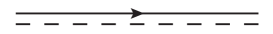
Figure 2: The propagator for $D^{*0}$ is represented by a double line (solid with an arrow and dashed). The Feynman rule for this propagator is given in Eq. (24). The propagator for $\bar{D}^{*0}$ looks like that for $D^{*0}$ with the arrow reversed.

Figure 3: The pair propagator is represented by a triple line (solid, dashed, and solid). The Feynman rule for this propagator is given in Eq. (37).

The Feynman rules for the propagators of $D^{0}$ or $\bar{D}^{0}$ and $\pi^{0}$ are

$$\boxed{\frac{i}{E-p^{2}/(2M)+i\epsilon},}$$ (23a)

$$\boxed{\frac{i}{E-p^{2}/(2m)+i\epsilon},}$$ (23b)

where $E$ is the kinetic energy of the particle and $\bm{p}$ is its momentum. The Feynman rule for the propagator of $D^{*0}$ or $\bar{D}^{*0}$ with vector indices $i$ and $j$ is

$$\boxed{\frac{i\,\delta^{ij}}{E-p^{2}/(2(M+m))-E_{*}},}$$ (24)

where $E$ is the energy of $D^{*0}$ relative to the $D^{0}\pi^{0}$ threshold, $\bm{p}$ is its momentum, and $E_{*}$ is the complex rest energy of $D^{*0}$ in Eq. (9). Galilean invariance requires the kinetic mass of $D^{*0}$ to be the sum $M+m$ of the kinetic masses of $D^{0}$ and $\pi^{0}$. Since $E_{*}$ has a negative imaginary part, an explicit $i\epsilon$ prescription is unnecessary in the $D^{*0}$ propagator in Eq. (24).

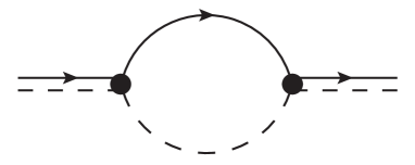
Figure 4: The 1-loop $D^{*0}$ self-energy diagram. This is the only $D^{*0}$ self-energy diagram in Galilean-invariant XEFT. The Feynman rule for the subdiagram with the external legs amputated is given in Eq. (26).

In XEFT beyond LO, there are corrections to the $D^{*0}$ propagator from interactions involving pions. The $D^{*0}$ self energy $\Sigma(E,p)$ is a function of its energy $E$ and its momentum $p$. In Galilean-invariant XEFT, the conservation of pion number implies that the exact $D^{*0}$ propagator can be calculated analytically by summing a geometric series in the 1-loop $D^{*0}$ self-energy diagram in Fig. 4. It is useful to have a Feynman rule for this subdiagram. Galilean invariance implies that the self-energy $\Sigma$ depends on $E$ and $p$ only through the invariant energy

$$E_{\rm rest}=E-\frac{p^{2}}{2(M+m)},$$ (25)

which is equal to the $D^{*0}$ energy in its rest frame. With dimensional regularization in $d$ spatial dimensions, the Feynman rule for the subdiagram in Fig. 4 with the $D^{*0}$ legs amputated is

$$\boxed{-i\,\Sigma(E_{\mathrm{rest}})\,\delta^{ij}=i\frac{4r^{2}g_{\pi}^{2}}{d}E_{\mathrm{rest}}\,I_{1}(E_{\mathrm{rest}})\,\delta^{ij},}$$ (26)

where $g_{\pi}^{2}$ is given in Eq. (13) and $r$ is the reduced-mass ratio in Eq. (11). The function $I_{1}(E)$ is given by a 1-loop momentum integral:

$$I_{1}(E)=\frac{\Gamma(1-d/2)}{(4\pi)^{d/2}}\Lambda^{3-d}\left[e^{-i\pi}2\mu_{\pi}E\right]^{d/2-1},$$ (27)

where $\Lambda$ is a renormalization scale with dimensions of momentum and $\mu_{\pi}$ is the $D^{0}\pi^{0}$ reduced mass in Eq. (10a). This loop integral has a linear ultraviolet divergence that is manifested as a pole in $d-2$. The analytic function $I_{1}(E)$ has a branch cut along the positive real $E$ axis. The complex phase inside the square brackets in Eq. (27) is chosen so that it gives the correct branch of the function when $E$ is near $\delta+i\epsilon$ on the first sheet and near $E_{*}$ on the second sheet.

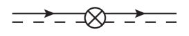
Figure 5: The $D^{*0}$ propagator counterterm vertex. Its Feynman rule is given in Eq. (28).

The $D^{*0}$ self-energy diagram in Fig. 4 has linear ultraviolet divergences. These divergences are cancelled by the $D^{*0}$ propagator counterterm vertex, which is illustrated in Fig. 5. A renormalization prescription for the $D^{*0}$ propagator can be expressed in terms of subtractions to the $D^{*0}$ self-energy. In the complex on-shell (COS) renormalization scheme for the $D^{*0}$ propagator, its pole in $E_{\mathrm{rest}}$ is at the complex value $E_{*}$ in Eq. (9) and the residue of that pole is the same as at LO. This requires the first two terms in the expansion of $\Sigma(E_{\rm rest})$ in powers of $E_{\rm rest}-E_{*}$ to be subtracted. The Feynman rule for the $D^{*0}$ propagator counterterm vertex in the COS scheme is

$$\boxed{i\big{[}\Sigma(E_{*})+\Sigma^{\prime}(E_{*})\,(E_{\mathrm{rest}}-E_{*})\big{]}\,\delta^{ij}=-i\frac{4r^{2}g_{\pi}^{2}}{d}I_{1}(E_{*})\left[E_{*}+\frac{d}{2}(E_{\mathrm{rest}}-E_{*})\right]\delta^{ij}.}$$ (28)

The Feynman rules for T-matrix elements include external-line factors for incoming and outgoing particles. For $D^{0}$, $\bar{D}^{0}$ and $\pi^{0}$, the external-line factors are simply 1. The corrections to the $D^{*0}$ propagator from interactions involving pions change the residue of the pole in the $D^{*0}$ propagator by a multiplicative factor $Z_{*}$. The external-line factor for $D^{*0}$ includes a residue factor $\sqrt{Z_{*}}$. In the COS scheme for the $D^{*0}$ propagator, $Z_{*}=1$. The external-line factor for an incoming $D^{*0}$ or $\bar{D}^{*0}$ with polarization vector $\bm{\varepsilon}$ and vector index $i$ is

$$\boxed{\varepsilon^{i}.}$$ (29)

The external-line factor for an outgoing $D^{*0}$ or $\bar{D}^{*0}$ is the same except that $\varepsilon^{i}$ is replaced by its complex conjugate.

IV.2 Pair propagator

If we use dimensional regularization with $d$ spatial dimensions, it is useful to introduce a renormalization scale $\Lambda$ to keep the dimensions of coupling constants the same as in the physical dimension $d=3$. This would have the effect of multiplying an interaction vertex with $n$ external lines by $n-2$ powers of $\Lambda^{(3-d)/2}$. In a Green function with $n$ external legs, the net effect of these powers of $\Lambda$ is a factor of $\Lambda^{3-d}$ for every loop integral and an overall multiplicative factor of $\Lambda^{(3-d)(n-2)/2}$. The factor of $\Lambda^{3-d}$ associated with a loop integral can be absorbed into its integration measure. If the Green function is made finite by renormalization, the overall multiplicative factor of $\Lambda^{(3-d)(n-2)/2}$ can simply be discarded, because it is equal to 1 in the physical dimension $d=3$. The resulting Feynman rules have no powers of $\Lambda$ in the vertices and the coupling constants have the same dimensions as in $d=3$.

In XEFT at LO, the only interaction term in the Lagrangian is the contact interaction term in Eq. (16) for $D^{*0}\bar{D}^{0}$ and $D^{0}\bar{D}^{*0}$ in the $C=+$ channel. The Feynman rule is the same for the four vertices for $D^{*0}\bar{D}^{0},D^{0}\bar{D}^{*0}\to D^{*0}\bar{D}^{0},D^{0}\bar{D}^{*0}$: $-i\big{(}1/\sqrt{2}\,\big{)}^{2}C_{0}\delta^{ij}$. The factors of $1/\sqrt{2}$ come from projecting a pair of charm mesons onto the $C=+$ channel. Two $C_{0}$ interactions can be connected by a $D^{*0}\bar{D}^{0}$ loop or a $D^{0}\bar{D}^{*0}$ loop. In Galilean-invariant XEFT, the loop integral is a function of the invariant energy of the pair of charm mesons:

$$E_{\mathrm{cm}}=E-\frac{P^{2}}{2(2M+m)},$$ (30)

where $E$ is their total energy relative to the $D^{*0}\bar{D}^{0}$ threshold and $\bm{P}$ is their total momentum. This invariant energy is equal to the total energy of the pair of charm mesons in their center-of-momentum (CM) frame. The sum of the two loop diagrams with two $C_{0}$ interactions can be expressed as the vertex multiplied by $-2\mu C_{0}\,J_{1}(E_{\mathrm{cm}})$, where the function $J_{1}(E)$ is defined by a 1-loop integral. Using dimensional regularization in $d$ spatial dimensions, the loop integral is

$$J_{1}(E)=\frac{\Gamma(1-d/2)}{(4\pi)^{d/2}}\Lambda^{3-d}\,\big{[}2\mu(E_{*}-E)\big{]}^{d/2-1},$$ (31)

where $\Lambda$ is the renormalization scale. This loop integral has a linear ultraviolet divergence that is manifested as a pole in $d-2$.

The $C_{0}$ interaction must be treated nonperturbatively in XEFT. The set of diagrams consisting of an arbitrary number of successive $C_{0}$ interactions connected by $D^{0}\bar{D}^{*0}$ or $D^{*0}\bar{D}^{0}$ loops is a geometric series that can be summed to all orders analytically. The factor in the resulting amplitude that depends on the invariant energy is a function ${\cal A}(E_{\mathrm{cm}})$ with dimensions 1/(momentum). In Ref. Braaten:2015tga , $(2\pi/\mu){\cal A}(E)$ was called the LO transition amplitude. In this paper, we refer to ${\cal A}(E)$ as the pair propagator, because it is equal to the propagator for the pair field $\bm{\phi}$ defined in Eq. (17) up to a constant multiplicative factor. If we use dimensional regularization in $d$ spatial dimensions, the pair propagator is

$${\cal A}(E)=\frac{1}{-2\pi/(\mu C_{0})-4\pi J_{1}(E)}.$$ (32)

Since $J_{1}(E)$ has a pole in $d-2$, this amplitude has a finite limit as $d\to 2$ only if $1/C_{0}$ also has a pole in $d-2$. The coupling constant $C_{0}$ can be tuned as a function of $d$ so that the LO transition amplitude has a finite limit as $d\to 3$:

$${\cal A}(E)=\frac{1}{-\gamma+\sqrt{-2\mu(E-E_{*})}}\qquad(d=3),$$ (33)

where $\gamma$ is an interaction parameter that we refer to as the LO binding momentum. A minimal choice for the dependence of $1/C_{0}$ on $d$ is that it is the sum of a pole in $d-2$ and a constant:

$$\frac{2\pi}{\mu C_{0}}=\left(\frac{2}{d-2}-2\right)\Lambda+\gamma.$$ (34)

In the limit $d\to 3$, $C_{0}$ approaches the finite value $2\pi/(\mu\gamma)$.

The pair propagator in Eq. (33) has a pole in the energy $E$ at the complex energy

$$E_{\mathrm{pole,LO}}=E_{*}-\gamma^{2}/(2\mu).$$ (35)

This LO pole energy has an imaginary part $-i\Gamma_{*0}/2$ from the $D^{*0}$ rest energy $E_{*}$ in Eq. (9). This imaginary part gives a contribution to the width of $X$ that can be interpreted as arising from its decays into $D^{0}\bar{D}^{0}\pi^{0}$ and $D^{0}\bar{D}^{0}\gamma$, which can proceed through the decay of a constituent $D^{*0}$ or $\bar{D}^{*0}$. But $X$ also has short-distance decay modes that do not involve decay of a constituent, such as $J/\psi\,\pi^{+}\pi^{-}$. The contribution to the imaginary part of the pole energy from these decays can only be taken into account through the imaginary part of $\gamma$ in Eq. (35). It is therefore convenient to take the LO binding momentum $\gamma$ to be a complex interaction parameter. Unitarity requires the positivity of $\mathrm{Im}[{\cal A}(E)]$ for real energy $E$, which requires $\mathrm{Im}[\gamma]$ to be positive. The real and imaginary parts of $\gamma$ are the only interaction parameters in XEFT at LO.

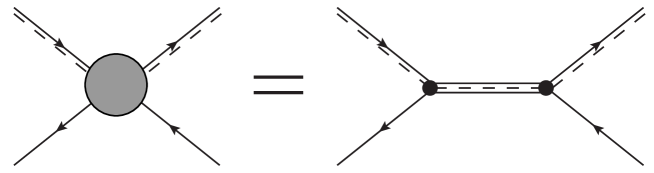
Figure 6: The $D^{*0}\bar{D}^{0}$-to-$D^{*0}\bar{D}^{0}$ vertex in Ref. Braaten:2015tga can be expressed as the product of a pair propagator and two vertices that connect the pair propagator to $D^{*0}\bar{D}^{0}$ legs.

The vertex corresponding to the LO transition amplitude is the same for the four transitions $D^{*0}\bar{D}^{0},D^{0}\bar{D}^{*0}\to D^{*0}\bar{D}^{0},D^{0}\bar{D}^{*0}$. In Ref. Braaten:2015tga , the vertex was represented by a blob, as in the diagram on the left side of Fig. 6. The Feynman rule for each of the four vertices is

$$+i\left(\frac{1}{\sqrt{2}}\right)^{2}\frac{2\pi}{\mu}\mathcal{A}(E_{\mathrm{cm}})\,\delta^{ij}.$$ (36)

It is convenient to express the $2\to 2$ vertex whose Feynman rule is given in Eq. (36) as the product of a $2\to 1$ vertex, the pair propagator, and a $1\to 2$ vertex, as illustrated in Fig. 6. The Feynman rule for the propagator of a pair with energy $E$, momentum $\bm{P}$, and vector indices $i$ and $j$ is

$$\boxed{-i\frac{2\pi}{\mu}\mathcal{A}(E_{\mathrm{cm}})\,\delta^{ij},}$$ (37)

where $E_{\mathrm{cm}}$ is the Galilean-invariant combination of $E$ and $P$ in Eq. (30). The vertices connecting $D^{*0}\bar{D}^{0}$ lines or $D^{0}\bar{D}^{*0}$ lines to a pair propagator are

$$\boxed{-i\frac{1}{\sqrt{2}}\,\delta^{ij}.}$$ (38)

The factor of $1/\sqrt{2}$ is the amplitude for the pair of charm mesons to be in the $C=+$ channel. The vertices connecting $D^{*0}\bar{D}^{0}$ lines to a pair propagator are illustrated in Fig. 7. It is easy to verify that the product of the pair propagator in Eq. (37) and two of the vertices in Eq. (38) reproduces the $2\to 2$ interaction vertex in Eq. (36).

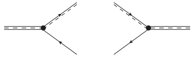
Figure 7: Vertices connecting $D^{*0}\bar{D}^{0}$ lines to a pair propagator. Their Feynman rules are given in Eq. (38).

The pair field defined in Eq. (17) can serve as an interpolating field for the $X$. The complete pair propagator that takes into account interactions beyond LO has the same form as in Eq. (37) but with $\mathcal{A}(E_{\mathrm{cm}})$ replaced by a more complicated function of the energy. An incoming or outgoing $X$ in a Feynman diagram can be represented by a triple line as in Fig. 3. The external-line factor for an incoming $X$ with polarization vector $\bm{\varepsilon}$ and vector index $i$ is

$$\boxed{\sqrt{Z_{X}}\,\varepsilon^{i},}$$ (39)

where $Z_{X}$ is the residue of the pole in $E_{\mathrm{cm}}$ of the coefficient of $i\,\delta^{ij}$ in the complete pair propagator analogous to Eq. (37). The external-line factor for an outgoing $X$ is the same except that $\varepsilon^{i}$ is replaced by its complex conjugate. The LO pole energy is the pole in the pair propagator $\mathcal{A}(E)$ in Eq. (32):

$$E_{\mathrm{pole}}=E_{*}-\frac{2\pi\,\Lambda^{2}}{\mu}\left(\frac{-2\pi/\mu}{\Gamma(1-d/2)\,\Lambda\,C_{0}}\right)^{2/(d-2)}.$$ (40)

If $C_{0}$ is replaced by the expression given by Eq. (34), the LO pole energy reduces to Eq. (35) in the limit $d\to 3$. At LO, $Z_{X}$ is the residue of the pole in $E$ of $-(2\pi/\mu)\mathcal{A}(E)$:

$$Z_{X,\mathrm{LO}}=\frac{4\pi^{2}\,\Lambda}{\Gamma(2-d/2)\,\mu^{2}}\left(\frac{-2\pi/\mu}{\Gamma(1-d/2)\,\Lambda\,C_{0}}\right)^{(4-d)/(d-2)}.$$ (41)

In the limit $d\to 3$, the LO residue factor reduces to

$$Z_{X,\mathrm{LO}}=2\pi\gamma/\mu^{2}\qquad(d=3).$$ (42)

IV.3 Pion interaction vertices

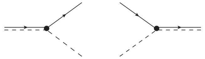
Figure 8: The vertices for the pionic transitions $D^{*0}\to D^{0}\pi^{0}$ and $D^{0}\pi^{0}\to D^{*0}$. The Feynman rules for the vertices are given in Eq. (43).

The charm mesons interact with pions in XEFT through the transitions $D^{*}\leftrightarrow D\pi$ and $\bar{D}^{*}\leftrightarrow\bar{D}\pi$. The vertices connecting $D^{*0}$ to $D^{0}\pi^{0}$ are illustrated in Fig. 8. The Feynman rules for the $D^{*0}\leftrightarrow D^{0}\pi^{0}$ and $\bar{D}^{*0}\leftrightarrow\bar{D}^{0}\pi^{0}$ vertices in Galilean-invariant XEFT are

$$\boxed{\pm\frac{g}{2\sqrt{m}f_{\pi}}\frac{(M\bm{q}-m\bm{p}_{0})^{i}}{M+m},}$$ (43)

where $\bm{q}$ and $\bm{p}_{0}$ are the momenta of $\pi^{0}$ and $D^{0}$ or $\bar{D}^{0}$, respectively. The overall sign is $+$ if the $D^{0}\pi^{0}$ or $\bar{D}^{0}\pi^{0}$ lines are outgoing and $-$ if they are incoming. In the $D^{0}\pi^{0}$ CM frame defined by $\bm{p}_{0}+\bm{q}=0$, the momentum-dependent factor in Eq. (43) reduces to $q^{i}$. This is the momentum-dependent factor in all frames in original XEFT.

IV.4 NLO interaction vertices

In this subsection, we present Feynman rules for NLO interaction vertices in Galilean-invariant XEFT whose legs include a pair propagator. The Feynman rules are given below as boxed expressions. They replace the Feynman rules for NLO interaction vertices in Ref. Braaten:2015tga .

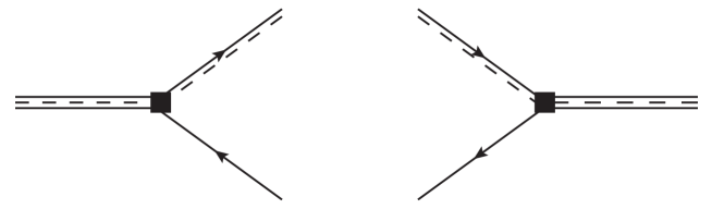
Figure 9: The $\nabla^{2}$ interaction vertices connecting $D^{*0}\bar{D}^{0}$ lines to a pair propagator. The Feynman rules for the vertices are given in Eq. (44).

The NLO $\nabla^{2}$ interaction terms in the Lagrangian are given in Eq. (20). The interaction vertices that connect $D^{*0}\bar{D}^{0}$ lines to a pair propagator are illustrated in Fig. 9. The Feynman rules for the corresponding vertices connecting $D^{*0}\bar{D}^{0}$ or $D^{0}\bar{D}^{*0}$ lines to a pair propagator are

$$\boxed{-i\frac{C_{2}}{2\sqrt{2}\,C_{0}}\frac{((M+m)\bm{p}_{0}-M\bm{p}_{1})^{2}}{(2M+m)^{2}}\,\delta^{ij},}$$ (44)

where $\bm{p}_{0}$ and $\bm{p}_{1}$ are the momenta of the spin-0 and spin-1 charm mesons. These four vertices replace the four $\nabla^{2}$ vertices in Ref. Braaten:2015tga that connect $D^{*0}\bar{D}^{0}$ or $D^{0}\bar{D}^{*0}$ lines to $D^{*0}\bar{D}^{0}$ or $D^{0}\bar{D}^{*0}$ lines. In the CM frame defined by $\bm{p}_{0}+\bm{p}_{1}=0$, the momentum-dependent factor in Eq. (44) reduces to $p_{0}^{2}$.

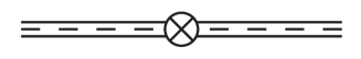
Figure 10: The pair-propagator counterterm vertex. The Feynman rule for the vertex is given in Eq. (45).

The NLO counterterm in the Lagrangian is given in Eq. (21). The pair-propagator counterterm vertex is illustrated in Fig. 10. Its Feynman rule is

$$\boxed{-i\frac{1}{C_{0}^{2}}\big{[}\delta C_{0}+D_{0}\,(E_{\mathrm{cm}}-E_{*})\big{]}\,\delta^{ij}.}$$ (45)

This vertex replaces the four counterterm vertices in Ref. Braaten:2015tga that connect $D^{*0}\bar{D}^{0}$ or $D^{0}\bar{D}^{*0}$ lines to $D^{*0}\bar{D}^{0}$ or $D^{0}\bar{D}^{*0}$ lines.

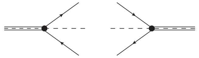
Figure 11: The $D\bar{D}\pi$ interaction vertices connecting $D^{0}\bar{D}^{0}\pi^{0}$ lines to a pair propagator. The Feynman rules for the vertices are given in Eq. (46).

The vertices connecting $D^{0}\bar{D}^{0}\pi^{0}$ lines to a pair propagator are illustrated in Fig. 11. The $D\bar{D}\pi$ interaction terms in the Lagrangian are given in Eq. (22). In Galilean-invariant XEFT, the Feynman rules for the vertices connecting a pair propagator to $D^{0}\bar{D}^{0}\pi^{0}$ lines are

$$\boxed{\pm\frac{B_{1}}{\sqrt{2m}\,C_{0}}\frac{(2M\bm{q}-m(\bm{p}_{0}+\bm{p}_{0}^{\prime}))^{i}}{2M+m},}$$ (46)

where $\bm{q}$, $\bm{p}_{0}$, and $\bm{p}_{0}^{\prime}$ are the momenta of $\pi^{0}$, $D^{0}$, and $\bar{D}^{0}$, respectively. The overall sign is $+$ if the $D^{0}\bar{D}^{0}\pi^{0}$ lines are outgoing and $-$ if they are incoming. In the CM frame defined by $\bm{p}_{0}+\bm{p}_{0}^{\prime}+\bm{q}=0$, the momentum-dependent factor in Eq. (46) reduces to $q^{i}$.

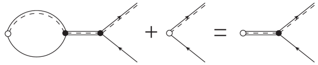
Figure 12: A diagrammatic identity that can be used to show that the Feynman rules in Ref. Braaten:2015tga give the same Green functions as the Feynman rules in this Section. The open circle on the left side is an arbitrary vertex that connects to $D^{*0}\bar{D}^{0}$ or $D^{0}\bar{D}^{*0}$ lines. The open circle on the right side is the corresponding vertex that connects to a pair propagator.

Calculations beyond LO using the Feynman rules for NLO interaction vertices presented above are simpler than calculations using the Feynman rules in Ref. Braaten:2015tga . There are sets of diagrams whose sums are the same with either set of Feynman rules. The Feynman rules above give the terms in such a sum more directly and with fewer UV divergences. The same terms can be obtained using the Feynman rules in Ref. Braaten:2015tga by using diagrammatic identities. An example of such a diagrammatic identity is shown in Fig. 12. The analytic expression for the identity is

$$J_{1}(E)\,\mathcal{A}(E)+\frac{1}{4\pi}=-\frac{1}{2\mu C_{0}}\mathcal{A}(E).$$ (47)

This identity follows from the expression for the LO transition amplitude in $d$ dimensions in Eq. (32). It allows the loop integral $J_{1}(E)$ to be cancelled against the loop integral in the denominator of the pair propagator $\mathcal{A}(E)$.

V NLO Pair Propagator

In this Section, we use Galilean-invariant XEFT to calculate the complete pair propagator to NLO.

V.1 Complete pair propagator

The pair propagator in XEFT at LO is given by the Feynman rule in Eq. (37), where the function $\mathcal{A}(E)$ in $d$ spatial dimensions is given in Eq. (32). In 3 dimensions, $\mathcal{A}(E)$ reduces to Eq. (33). In XEFT beyond LO, there are corrections to the pair propagator from interactions involving pions and from other interactions. The corrections to the pair propagator can be organized into a geometric series of pair self-energy diagrams. The complete pair propagator is obtained by summing the geometric series. It can be expressed in the form

$$-i\frac{2\pi}{\mu}\frac{1}{\mathcal{A}(E_{\mathrm{cm}})^{-1}-\Pi_{0}(E_{\mathrm{cm}})}\,\delta^{ij},$$ (48)

where $\Pi_{0}(E)$ is a function with dimensions of momentum that we call the pair self-energy.

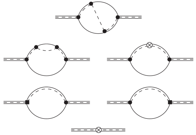
Figure 13: The NLO diagrams for the pair self-energy. The sum of the amputated diagrams is $i[\mu/(2\pi)]\,\Pi_{0}(E)\,\delta^{ij}$.

The NLO diagrams for the pair self-energy are shown in Fig. 13. The expressions for those diagrams can be obtained from Appendix B, in which the NLO diagrams for the transition amplitude for $D^{*0}\bar{D}^{0}\to D^{*0}\bar{D}^{0}$ are calculated. Some of the diagrams for $D^{*0}\bar{D}^{0}\to D^{*0}\bar{D}^{0}$ have pair self-energy subdiagrams. The expression for each pair self-energy subdiagram can be obtained by removing the initial and final vertex factors and the two pair propagators from the diagram for $D^{*0}\bar{D}^{0}\to D^{*0}\bar{D}^{0}$. The NLO pair self-energy can be expressed as

$$\Pi_{0}(E)=g_{\pi}^{2}\,F(E)+(C_{2}/C_{0})H(E)-(2\pi/(\mu C_{0}^{2}))\big{[}\delta C_{0}+D_{0}(E-E_{*})\big{]}.$$ (49)

The functions $F(E)$ and $H(E)$ can be expressed in terms of the 1-loop integrals $J_{n}$ and $I_{n}$ and the 2-loop integrals $K_{lmn}$ defined in Appendix A. The function $F(E)$, which has dimensions of (momentum)², comes from the first two rows of diagrams in Fig. 13. It can be obtained from the 2-loop pion-exchange diagram in Eq. (145) and the $D^{*}$ propagator correction diagrams in Eqs. (148) and (149):

$$F(E) = -\frac{8\pi r}{d}\bigg{(}\frac{1}{\sqrt{1-r}}\big{[}2K_{110}(E)-2(2\mu E_{*}-r\mu E)K_{111}(E)-(2-r)J_{1}(E)^{2}\big{]}$$ (50)

$$\hskip 14.22636pt+2K_{110}(E)-4\mu E_{*}\big{[}K_{120}(E)-rI_{1}(E_{*})J_{2}(E)\big{]}-drI_{1}(E_{*})J_{1}(E)\bigg{)},$$

where $r=\mu_{\pi}/\mu$ is the ratio of reduced masses defined in Eq. (11). The function $H(E)$, which has dimensions of (momentum)³, comes from the third row of diagrams in Fig. 13. It can be obtained from the 1-loop $\nabla^{2}$ vertex diagrams in Eq. (152):

$$H(E) = 8\pi\mu(E-E_{*})\,J_{1}(E).$$ (51)

The $\delta C_{0}$ and $D_{0}$ terms in Eq. (49) come from the last diagram in Fig. 13. They can be obtained from the pair-propagator counterterm diagram in Eq. (153).

V.2 Renormalization

The renormalizability of XEFT as an effective field theory requires that ultraviolet (UV) divergences can be cancelled order by order in the power counting by renormalization of the parameters of XEFT. With dimensional regularization, the UV divergences in loop integrals produce poles in $d-2$ and poles in $d-3$. A pole in $d-3$ represents a logarithmic UV divergence, and a pole in $d-2$ represents a linear UV divergence. In the previous calculations in XEFT at NLO in Refs. Fleming:2007rp ; Jansen:2013cba ; Dai:2019hrf , power divergence subtraction was used to remove the poles in $d-2$. The subsequent limit $d\to 3$ produces terms with positive integer powers of the renormalization scale $\Lambda$. It may also produce terms that depend logarithmically on $\Lambda$. If power divergence subtraction is used to make linear UV divergences explicit in the limit $d\to 3$, renormalization must remove both the poles in $d-3$ and the dependence on $\Lambda$.

The Green functions in XEFT should be multiplicatively renormalizable. A renormalized amputated connected Green function can be defined by multiplying the amputated connected Green function by an appropriate renormalization factor $\sqrt{Z}$ for every external leg. For $D^{0}$ and $\bar{D}^{0}$ legs, the renormalization constant is $Z=1$. For $D^{*0}$ and $\bar{D}^{*0}$ legs, the renormalization constant in the COS scheme for the $D^{*0}$ propagator is $Z_{*}=1$. When the Lagrangian for XEFT is formulated using the pair field $\bm{\phi}$ as in Section III, there are also Green functions with external pair legs. We denote the corresponding dimensionless renormalization constant by $Z_{\phi}$. It is equal to 1 at LO, but $Z_{\phi}$ has corrections beyond LO.

The renormalized complete pair propagator differs from the complete pair propagator in Eq. (48) by a multiplicative factor $1/Z_{\phi}$. The renormalized pair self-energy $\Pi(E)$ can be defined by

$$Z_{\phi}\big{[}\mathcal{A}(E)^{-1}-\Pi_{0}(E)\big{]}=\mathcal{A}(E)^{-1}-\Pi(E).$$ (52)

The renormalization constant at NLO can be expressed as $Z_{\phi}=1+\delta Z_{\phi}$. The renormalized pair self-energy at NLO is

$$\Pi(E) = g_{\pi}^{2}\,F(E)+(C_{2}/C_{0})\,H(E)$$ (53)

$$-(2\pi/(\mu C_{0}^{2}))\big{[}\delta C_{0}+D_{0}\,(E-E_{*})\big{]}-\delta Z_{\phi}\,\mathcal{A}(E)^{-1}.$$

It must be possible to choose $\delta Z_{\phi}$ so the linear and logarithmic UV divergences in this expression all cancel.

We first consider the poles in $d-2$ in the renormalized NLO pair self-energy $\Pi(E)$ in Eq. (53). The poles in $d-2$ for the loop integrals are given in subsection A.3 of Appendix A. The function $F(E)$ in Eq. (50) has double poles in $d-2$ from the 2-loop integral $K_{110}$ and from the products of 1-loop integrals $J_{1}^{2}$ and $I_{1}J_{1}$. Along with the double poles, which do not depend on $E$, there are single poles whose coefficients include a logarithm of the form $\log(E_{*}-E)$. There are also canceling single poles in $d-2$ in the combination $K_{120}-rI_{1}J_{2}$. The double poles and the constant single poles in $F(E)$ can be cancelled by the counterterm $\delta C_{0}$ in Eq. (53). The function $H(E)$ in Eq. (51), which has a factor $E-E_{*}$, has a single pole in $d-2$ from the loop integral $J_{1}$. The single pole can be cancelled by the counterterm $D_{0}$ in Eq. (53). The poles in $d-2$ from the loop integrals in $\Pi(E)$ that cannot be cancelled by the counterterms $\delta C_{0}$ and $D_{0}$ are the single poles with energy dependence $\log(E_{*}-E)$. The sum of these terms and the $\delta Z_{\phi}$ term in Eq. (53) are

$$\frac{2r\sqrt{1-r}\,g_{\pi}^{2}\Lambda^{2}}{(d-2)\pi}\log\frac{2\mu(E_{*}-E)}{\Lambda^{2}}-\delta Z_{\phi}\,\mathcal{A}(E)^{-1}.$$ (54)

The argument of the logarithm has been made dimensionless by using the renormalization scale $\Lambda$. The expression for the amplitude $\mathcal{A}(E)$ in Eq. (32) in the limit $d\to 2$ is

$$\lim_{d\to 2}\mathcal{A}(E)=\frac{1/\Lambda}{\log\big{(}2\mu(E_{*}-E)/\Lambda_{2}^{2}\big{)}},$$ (55)

where the momentum scale $\Lambda_{2}$ in the logarithm is determined by the constant under the pole in $d-2$ of $C_{0}^{-1}$. The dependence on $E$ cancels between the two terms in Eq. (54) if $\delta Z_{\phi}$ has a pole in $d-2$ with the appropriate residue. The renormalization constant at NLO must have the form

$$Z_{\phi}=1+\left(\frac{2r\sqrt{1-r}\,g_{\pi}^{2}\,\Lambda}{(d-2)\pi}+\mathrm{finite}\right),$$ (56)

where the finite NLO term has a finite limit as $d\to 2$. The cancellation of the $\log(E-E_{*})$ terms leaves a single pole with a factor $\log(\Lambda_{2}^{2}/\Lambda^{2})$ that can be cancelled by the counterterm $\delta C_{0}$. We conclude that all the poles in $d-2$ in the NLO pair self-energy can be cancelled by the counterterms $\delta C_{0}$ and $D_{0}$.

Having verified that all the linear UV divergences in the renormalized pair self-energy can be cancelled by the counterterms $\delta C_{0}$ and $D_{0}$ there is nothing to be gained by making them explicit using power divergence subtraction. We therefore choose to simplify intermediate results by using conventional dimensional regularization in which the only explicit UV divergences are poles in $d-3$.

We now consider the poles in $d-3$ in the renormalized NLO pair self-energy $\Pi(E)$ in Eq. (53). The poles in $d-3$ for the loop integrals are given in subsection A.5 of Appendix A. The only poles in $d-3$ come from the 2-loop integrals $K_{110}$, $K_{120}$, and $K_{111}$ in the function $F(E)$ in Eq. (50). The poles in $K_{120}$ and $K_{111}$ are constants. The pole in $K_{110}$ is a linear function of $E$. Thus all the poles in $d-3$ can be cancelled by the counterterms $\delta C_{0}$ and $D_{0}$. We conclude that the logarithmic UV divergences in the NLO pair self-energy can be cancelled by these counterterms.

V.3 Minimal subtraction renormalization scheme

We have verified that the linear and logarithmic UV divergences in the NLO pair self-energy can be cancelled by the counterterms $\delta C_{0}$ and $D_{0}$ and the NLO term $\delta Z_{\phi}$ in the pair renormalization constant. A renormalization scheme for $D^{*0}\bar{D}^{0}$ and $D^{0}\bar{D}^{*0}$ amplitudes in XEFT corresponds to a specific choice for those counterterms. The simplest renormalization scheme is the minimal subtraction (MS) scheme, in which $\delta C_{0}$, $D_{0}$, and $\delta Z_{\phi}$ are chosen to cancel only the poles in $d-3$. Since $\delta Z_{\phi}$ has a pole in $d-2$ but no poles in $d-3$, $\delta Z_{\phi}=0$ in the MS scheme. At NLO, the poles in $d-3$ in the pair propagator appear only in the function $F(E)$ in Eq. (50). The explicit form of the poles in $d-3$ of $F(E)$ is

$$\big{[}F(E)\big{]}_{\mathrm{pole}} = \frac{r^{2}}{3\pi^{2}(d-3)}\Bigg{\{}\left[\left(\frac{1}{\sqrt{1-r}}+3\right)\sqrt{r}-\frac{2-r}{1-r}\arccos\big{(}\sqrt{r}\,\big{)}\right]\mu E_{*}$$ (57)

$$\hskip 71.13188pt-\left[\left(\frac{1}{\sqrt{1-r}}+1\right)\sqrt{r}-\frac{r}{1-r}\arccos\big{(}\sqrt{r}\,\big{)}\right]\mu(E-E_{*})\bigg{\}}.~{}~{}~{}$$

A pole in $d-3$ of $F(E)$ is accompanied by the logarithm $\log(2\mu E_{*}/\bar{\Lambda}^{2})$, where $\bar{\Lambda}$ is a renormalization scale. In the MS scheme, the cancellation of the poles in $d-3$ by the counterterms leaves terms in $F(E)$ that depend on $\bar{\Lambda}$. They can be obtained by replacing $1/(d-3)$ in Eq. (57) by $\log(2\mu E_{*}/\bar{\Lambda}^{2})$. The logarithm multiplying the constant $\mu E_{*}$ term can be absorbed into an NLO correction to the LO parameter $\gamma$. However there is also a logarithm multiplying the $\mu(E-E_{*})$ term. The renormalization scale $\bar{\Lambda}$ in this logarithm can be interpreted as an additional real-valued interaction parameter in the MS scheme associated with renormalization of the coupling constant $D_{0}$. The existence of this additional interaction parameter was not recognized in Ref. Braaten:2015tga .

V.4 Complex threshold renormalization scheme

We introduce a new renormalization scheme for $D^{*0}\bar{D}^{0}$ and $D^{0}\bar{D}^{*0}$ amplitudes in XEFT that we call the complex threshold (CT) renormalization scheme. It is defined by specifying the behavior of the renormalized pair propagator near the complex threshold $E=E_{*}$. The renormalized inverse pair propagator has a threshold expansion in half-integer powers of $E-E_{*}$ or, equivalently, in integer powers of the function $\kappa(E)$ defined by

$$\kappa(E)=\sqrt{2\mu(E_{*}-E)}.$$ (58)

The CT scheme is partly defined by specifying the first two leading terms in the threshold expansion:

$$\mathcal{A}(E)^{-1}-\Pi(E)=-\gamma+\kappa(E)+\mathcal{O}\big{(}\kappa^{2}(E)\big{)}.$$ (59)

At NLO, the definition of the CT scheme is completed by specifying the real part of the coefficient of $\kappa^{2}(E)$ in the threshold expansion of $\Pi(E)$. We choose to denote that real part by $F_{2}g_{\pi}^{2}$, where $F_{2}$ is a dimensionless adjustable interaction parameter. At higher orders, the definition of the CT scheme may need to be extended by specifying the real parts of coefficients of higher integer powers of $\kappa^{2}(E)$.

We proceed to obtain a more explicit expression for the renormalized NLO pair self-energy $\Pi(E)$ in the limit $d\to 3$. The expression for $\Pi(E)$ in Eq. (53) depends on the functions $F(E)$ and $H(E)$, which are expressed in terms of loop integrals in Eqs. (50) and (51). The threshold expansions in powers of $E-E_{*}$ of the loop integrals in Ref. Braaten:2015tga are given in subsection A.6 of Appendix A. In the limit $d\to 3$, the function $H(E)$ is very simple:

$$H(E)=\kappa^{3}(E).$$ (60)

In the limit $d\to 3$, the function $F(E)$ can be expanded in integer powers of $\kappa(E)$:

$$F(E)=f_{0}\,\kappa_{*}^{2}+f_{1}\,\kappa_{*}\kappa(E)+f_{2}\,\kappa^{2}(E)+f_{4}\,\kappa^{4}(E)/\kappa_{*}^{2}+\ldots.$$ (61)

where $\kappa_{*}=\sqrt{2\mu E_{*}}$. The dimensionless coefficients $f_{n}$ are functions of the reduced-mass ratio $r=\mu_{\pi}/\mu$. The $f_{1}$ term is the only one with an odd power of $\kappa(E)$. The coefficient $f_{1}$ is pure imaginary, and it is suppressed by a factor of $r^{5/2}$:

$$f_{1}=i\frac{r^{5/2}}{3\pi\sqrt{1-r}}.$$ (62)

The coefficients $f_{0}$ and $f_{2}$ have single poles in $d-3$, and they have finite imaginary parts:

$$\mathrm{Im}[f_{0}] = \frac{r^{2}}{6\pi}\left[\frac{2-r}{1-r}\arccos\big{(}\sqrt{r}\,\big{)}-\left(3+\frac{1}{\sqrt{1-r}}\right)\sqrt{r}\right],$$ (63a)

$$\mathrm{Im}[f_{2}] = -\frac{r^{5/2}}{6\pi}\left[1+\frac{1}{\sqrt{1-r}}-\frac{\sqrt{r}}{1-r}\arccos\big{(}\sqrt{r}\,\big{)}\right].$$ (63b)

All the higher coefficients have finite limits as $d\to 3$, and they are real valued. The coefficients $f_{n}$ with $n\geq 2$ can be expressed analytically in terms of hypergeometric functions. The coefficient $f_{4}$ is

$$f_{4} = \frac{2(2-r)}{3\pi^{2}\sqrt{1-r}}\bigg{(}{}_{2}F_{1}\big{(}\mathrm{-}\tfrac{1}{2},\mathrm{-}\tfrac{1}{2},\tfrac{3}{2};1-r\big{)}+\frac{2-4r-r^{2}}{8\sqrt{1-r}}\,\arccos\big{(}\sqrt{r}\big{)}$$ (64)

$$\hskip 85.35826pt+\frac{(12-22r-5r^{2})\sqrt{r}}{24(2-r)}-\frac{\sqrt{1-r}\,r^{5/2}}{40(2-r)}\bigg{)}.$$

Its value in the limit $r\to 0$ is $f_{4}=2/(3\pi)$. Its numerical value at $r=0.1304$ is $f_{4}=0.1979$. The renormalized NLO pair self-energy in Eq. (53) can be expressed as

$$\Pi(E) = \big{[}f_{0}g_{\pi}^{2}\kappa_{*}^{2}-2\pi\delta C_{0}/(\mu C_{0}^{2})+\delta Z_{\phi}\gamma\big{]}+\big{[}f_{1}g_{\pi}^{2}\kappa_{*}-\delta Z_{\phi}\big{]}\kappa(E)$$ (65)

$$+\big{[}f_{2}g_{\pi}^{2}+\pi D_{0}/(\mu^{2}C_{0}^{2})\big{]}\kappa^{2}(E)+(C_{2}/C_{0})\,\kappa^{3}(E)+g_{\pi}^{2}\,F_{4}(E),$$

where $F_{4}(E)$ is obtained by subtracting from $F(E)$ the first three terms in its expansion in powers of $\kappa(E)$:

$$F_{4}(E)=F(E)-\big{[}f_{0}\,\kappa_{*}^{2}+f_{1}\,\kappa_{*}\kappa(E)+f_{2}\,\kappa^{2}(E)\big{]}.$$ (66)

It has a threshold expansion in even powers of $\kappa(E)$ that begins with a $\kappa^{4}(E)$ term.

We proceed to implement the CT scheme for the complete pair propagator at NLO. The first four terms in the threshold expansion for the NLO renormalized pair self-energy $\Pi(E)$ are already explicit in Eq. (65). There are poles in $d-3$ in the coefficients $f_{0}$ and $f_{2}$. The CT scheme requires the total subtraction of the leading term and the $\kappa(E)$ term in Eq. (65) and the partial subtraction of the $\kappa^{2}(E)$ term.

We first consider the $\kappa(E)$ term in the threshold expansion for $\Pi(E)$ in Eq. (65). The total subtraction of the $\kappa(E)$ term requires $\delta Z_{\phi}=f_{1}g_{\pi}^{2}\kappa_{*}$. The coefficient $f_{1}$ is finite at $d=3$ and pure imaginary. The resulting expression for the renormalization constant $Z_{\phi}$ in the CT scheme is

$$Z_{\phi}=1+i\frac{r^{5/2}}{3\pi\sqrt{1-r}}g_{\pi}^{2}\kappa_{*}\quad(d=3).$$ (67)

If we include in $\delta Z_{\phi}$ the pole in $d-2$ in Eq. (56), we must also include an additional finite term that cancels that pole term at $d=3$, so that $Z_{\phi}$ in the limit $d\to 3$ is again given by Eq. (67). Since the finite renormalization in Eq. (67) is not an essential aspect of the CT scheme, we will continue to regard $\delta Z_{\phi}$ as arbitrary.

We next consider the leading term in the threshold expansion for $\Pi(E)$ in Eq. (65). The NLO binding momentum with $\delta Z_{\phi}=f_{1}g_{\pi}^{2}\kappa_{*}$ is

$$\gamma_{\mathrm{NLO}}=\gamma+f_{1}\,g_{\pi}^{2}\kappa_{*}\gamma+f_{0}\,g_{\pi}^{2}\kappa_{*}^{2}-2\pi\delta C_{0}/(\mu C_{0}^{2}),$$ (68)

where $f_{1}$ is given in Eq. (62) and the imaginary part of $f_{0}$ is given in Eq. (63a). The terms $f_{1}\,g_{\pi}^{2}\kappa_{*}\gamma$ and $i\,\mathrm{Im}[f_{0}]\,g_{\pi}^{2}\kappa_{*}^{2}$ give positive contributions to the imaginary part of $\gamma_{\mathrm{NLO}}$. These contributions, which take into account the decay of $X$ into $D^{0}\bar{D}^{0}\pi^{0}$, add to the imaginary part of $\gamma$, which takes into account short-distance decays of $X$, such as its decay into $J/\psi\,\pi^{+}\pi^{-}$. The counterterm $\delta C_{0}$ must cancel the pole in $d-3$ from the coefficient $f_{0}$ in Eq. (68). It could be chosen to cancel also the real finite part of $f_{0}$. The CT scheme requires the total subtraction of the leading term in Eq. (65), which implies $\gamma_{\mathrm{NLO}}=\gamma$.

We finally consider the $\kappa^{2}(E)$ term in the threshold expansion for $\Pi(E)$ in Eq. (65). The counterterm $D_{0}$ must cancel the pole in $d-3$ from the coefficient $f_{2}$ in Eq. (65). It can be chosen to also cancel an arbitrary real part of $f_{2}$. We denote the remaining finite real part of that coefficient by $F_{2}$. The resulting expression for the renormalized pair self-energy at NLO is

$$\Pi(E)=\big{[}f_{1}g_{\pi}^{2}\kappa_{*}-\delta Z_{\phi}\big{]}\kappa(E)+\big{(}F_{2}+i\,\mathrm{Im}[f_{2}]\big{)}g_{\pi}^{2}\,\kappa^{2}(E)+(C_{2}/C_{0})\,\kappa^{3}(E)+g_{\pi}^{2}\,F_{4}(E).$$ (69)

In the CT scheme, the term proportional to $\kappa(E)$ is absent. The adjustable real interactions parameters in XEFT at NLO in the CT scheme are $\mathrm{Re}[\gamma]$, $\mathrm{Im}[\gamma]$, $F_{2}$, and $C_{2}/C_{0}$. The existence of the additional interaction parameter $F_{2}$ was not recognized in Ref. Braaten:2015tga .

V.5 Other previous renormalization schemes

In Refs. Fleming:2007rp ; Dai:2019hrf , the differential decay rate of the $X$ into $D^{0}\bar{D}^{0}\pi^{0}$ was calculated to NLO in original XEFT. The LO binding momentum $\gamma$ was taken to be a real adjustable parameter. The calculation of the NLO diagrams did not produce any poles in $d-3$. Power divergence subtraction was used to make the poles in $d-2$ explicit as dependence on the renormalization scale $\Lambda$, which was denoted by $\Lambda_{\mathrm{PDS}}/2$. The pair propagator $\mathcal{A}(E)$ in $d$ dimensions is given in Eq. (32). If the pole in $d-2$ is subtracted from the loop integral $J_{1}(E)$ in Eq. (31), then the pole in $d-2$ must also be subtracted from $2\pi/(\mu C_{0})$ in Eq. (34). The resulting expression for $C_{0}$ satisfies

$$C_{0}\,(2\Lambda-\gamma)=-2\pi/\mu.$$ (70)

In Refs. Fleming:2007rp ; Dai:2019hrf , the remaining dependence on the renormalization scale appeared in the following combinations:

$$C_{2}\,(2\Lambda-\gamma)^{2}=(\pi/\mu)\,R_{0},$$ (71a)

$$\big{[}B_{1}+(g\mu/f_{\pi})C_{2}\big{]}\,(2\Lambda-\gamma)=\eta/(100~{}\mathrm{MeV})^{3}.$$ (71b)

These equations defined two renormalized interaction parameters: $R_{0}$ (denoted by $r_{0}$ in Ref. Fleming:2007rp ), which has dimensions 1/(momentum), and $\eta$, which is dimensionless. In Refs. Fleming:2007rp ; Dai:2019hrf , $R_{0}$ was assumed to be positive and less than $1/(100\,\mathrm{MeV})$ and $\eta$ was assumed to be in the range $|\eta|<1$.

In our calculations, we have chosen not to make linear UV divergences manifest by using power divergence subtraction. The same results could be obtained by using power divergence subtraction and then setting $\Lambda=0$. If we divide Eq. (71a) by Eq. (70) and then set $\Lambda=0$, we find

$$C_{2}/C_{0}=R_{0}/(2\gamma).$$ (72)

Thus we can replace $C_{2}/C_{0}$ in our NLO corrections by $R_{0}/(2\gamma)$, where $R_{0}$ is the renormalized interaction parameter introduced in Ref. Fleming:2007rp .

In Ref. Jansen:2013cba , the $D^{*0}\bar{D}^{0}$ scattering length was calculated to NLO in original XEFT. In addition to terms proportional to $\Lambda$, $\Lambda^{2}$, $\log\Lambda$, there was explicit dependence on $\Lambda$ from terms proportional to $1/(2\Lambda-\gamma)$. These terms were introduced by a resummation prescription for dealing with an infrared divergence at the $D^{*0}\bar{D}^{0}$ threshold. The terms proportional to $1/(2\Lambda-\gamma)$ were not removed by the renormalization of the parameters. This failure of the renormalization procedure suggests that the resummation prescription for the infrared divergences in Ref. Jansen:2013cba was incompatible with the renormalization prescription.

In Ref. Braaten:2015tga , which introduced Galilean invariant XEFT, a renormalization prescription for $D^{*0}\bar{D}^{0}$ and $D^{0}\bar{D}^{*0}$ amplitudes called the complex on-shell (COS) renormalization scheme was introduced. The COS scheme requires the pole in the energy and the residue of the pole in the $D^{*0}\bar{D}^{0}$ transition amplitude to be the same as at LO. This renormalization scheme will be discussed in Section VI.3 after the NLO calculation of the $D^{*0}\bar{D}^{0}$ transition amplitude.

V.6 NLO pole energy

The complete pair propagator $\Pi(E)$ has a pole in $E$ at a complex energy that is conveniently expressed as

$$E_{\mathrm{pole}}=E_{*}-\gamma_{X}^{2}/(2\mu),$$ (73)

where $\gamma_{X}$ is the complex binding momentum. The pole energy at NLO in the CT scheme is a zero of the renormalized inverse pair propagator $-\gamma+\kappa(E)-\Pi(E)$, where $\Pi(E)$ is given in Eq. (69). The equation for $\gamma_{X}$ at NLO can be obtained by substituting $E\to E_{\mathrm{pole}}$ in the expression for $\Pi(E)$ and then setting it equal to $-\gamma+\gamma_{X}$. The equation can be expressed as

$$\gamma_{X}=\gamma+\big{[}f_{1}g_{\pi}^{2}\kappa_{*}-\delta Z_{\phi}\big{]}\gamma_{X}+\big{(}F_{2}+i\,\mathrm{Im}[f_{2}]\big{)}\,g_{\pi}^{2}\gamma_{X}^{2}+\frac{R_{0}}{2\gamma}\,\gamma_{X}^{3}+g_{\pi}^{2}\,F_{4}\big{(}E_{*}-\gamma_{X}^{2}/(2\mu)\big{)}.$$ (74)

In the CT scheme, the term on the right side proportional to $\gamma_{X}$ is zero. We have used Eq. (72) to set $C_{2}/C_{0}=R_{0}/(2\gamma)$. The equation for $\gamma_{X}$ can be solved as an expansion in powers of $\gamma$. The solution for the first few terms in the CT scheme is

$$\gamma_{X} = \gamma+\tfrac{1}{2}\big{[}R_{0}+2\big{(}F_{2}+i\,\mathrm{Im}[f_{2}]\big{)}g_{\pi}^{2}\big{]}\gamma^{2}$$ (75)

$$\hskip 14.22636pt+\tfrac{3}{4}\big{[}R_{0}+2\big{(}F_{2}+i\,\mathrm{Im}[f_{2}]\big{)}g_{\pi}^{2}\big{]}\big{[}R_{0}+\tfrac{4}{3}\big{(}F_{2}+i\,\mathrm{Im}[f_{2}]\big{)}g_{\pi}^{2}\big{]}\gamma^{3}+\ldots.$$

In the calculation of the rate for a reaction with $X$ as an incoming or outgoing particle, the T-matrix element has a factor $\sqrt{Z_{X}}$ for the $X$. The residue factor $Z_{X}$ is determined by the derivative with respect to $E$ of the renormalized inverse pair propagator in Eq. (52) evaluated at $E_{\mathrm{pole}}$. The reciprocal of the residue factor can be expressed as

$$Z_{X}^{-1}=Z_{X,\mathrm{LO}}^{-1}+\big{(}\mu/(2\pi)\big{)}\,\Pi^{\prime}(E_{\mathrm{pole}}),$$ (76)

where $Z_{X,\mathrm{LO}}$ is the LO residue factor in Eq. (41). The NLO pair self-energy $\Pi(E)$ is given in Eq. (69). The reciprocal of the residue factor at NLO in the limit $d\to 3$ is

$$Z_{X,\mathrm{NLO}}^{-1} = \frac{\mu^{2}}{2\pi}\bigg{[}\frac{1}{\gamma}-\big{(}f_{1}g_{\pi}^{2}\kappa_{*}-\delta Z_{\phi}\big{)}\frac{1}{\gamma_{X}}-2\big{(}F_{2}+i\,\mathrm{Im}[f_{2}]\big{)}\,g_{\pi}^{2}$$ (77)

$$\hskip 28.45274pt-\frac{3}{2}\frac{R_{0}\,\gamma_{X}}{\gamma}+\frac{g_{\pi}^{2}}{\mu}F_{4}^{\prime}\big{(}E_{*}-\gamma_{X}^{2}/(2\mu)\big{)}\bigg{]}\qquad(d=3).$$

Note that the choice $Z_{\phi}=f_{1}g_{\pi}^{2}\kappa_{*}$ in the CT scheme simplifies both the equation for the binding momentum in Eq. (74) and Eq. (77) for the residue factor.

VI $\bm{D^{*0}\bar{D}^{0}}$ Scattering

In this Section, we use Galilean-invariant XEFT to calculate the $D^{*0}\bar{D}^{0}$ elastic scattering amplitude to NLO and we discuss the breakdown of the effective range expansion.

VI.1 NLO transition amplitude

The amputated connected Green function for $D^{*0}\bar{D}^{0}\to D^{*0}\bar{D}^{0}$ is a tensor $\mathcal{T}^{ij}$ whose vector indices are those of the incoming and outgoing $D^{*0}$ lines. If the incoming and outgoing $\bar{D}^{0}$ are on their energy shells but the incoming and outgoing $D^{*0}$ are off their energy shells, this transition tensor $\mathcal{T}^{ij}(E,\bm{p},\bm{p}^{\prime})$ is a function of the total energy $E$ of the pair of charm mesons in their CM frame and the relative momenta $\bm{p}$ and $\bm{p}^{\prime}$ of the incoming and outgoing charm mesons. The transition tensor $\mathcal{T}_{+}^{ij}$ for the $C=+$ channel is the sum of the transition tensors for $D^{*0}\bar{D}^{0}\to D^{*0}\bar{D}^{0}$, $D^{*0}\bar{D}^{0}\to D^{0}\bar{D}^{*0}$, $D^{0}\bar{D}^{*0}\to D^{*0}\bar{D}^{0}$, and $D^{0}\bar{D}^{*0}\to D^{0}\bar{D}^{*0}$ multiplied by 1/2. The S-wave contribution to the transition tensor can be obtained by averaging over the directions of $\bm{p}$ and $\bm{p}^{\prime}$. It is diagonal in the vector indices $i$ and $j$, and it is a function of $E$, $p$, and $p^{\prime}$. The $C=+$ S-wave transition tensor can be expressed in the form

$$\Big{\langle}\mathcal{T}_{+}^{ij}(E,\bm{p},\bm{p}^{\prime})\Big{\rangle}_{\bm{\hat{p}},\bm{\hat{p}}^{\prime}}=\frac{2\pi}{\mu}\mathcal{A}_{s+}(E,p,p^{\prime})\,\delta^{ij},$$ (78)

where the scalar transition amplitude $\mathcal{A}_{s+}$ has dimensions 1/momentum. At LO, the $C=+$ S-wave transition amplitude reduces to the pair propagator $\mathcal{A}(E)$ in Eq. (33).

The NLO diagrams for the transition tensor for $D^{*0}\bar{D}^{0}\to D^{*0}\bar{D}^{0}$ are calculated in Appendix B. There are three pion-exchange diagrams shown in Fig. 14: two 1-loop diagrams and a 2-loop diagram. There are two $D^{*}$ propagator correction diagrams shown in Fig. 16: a 2-loop diagram with a $D^{*}$ self-energy subdiagram and a 1-loop diagram with a $D^{*}$ self-energy counterterm. With the Feynman rules for NLO interaction vertices in Section IV.4, there are four $\nabla^{2}$ vertex diagrams in Fig. 17: two tree diagrams and two 1-loop diagrams. There is also a tree diagram with a pair-propagator counterterm vertex in Fig. 18. There are analogous diagrams for the other three amplitudes $D^{*0}\bar{D}^{0}\to D^{0}\bar{D}^{*0}$, $D^{0}\bar{D}^{*0}\to D^{*0}\bar{D}^{0}$, and $D^{0}\bar{D}^{*0}\to D^{0}\bar{D}^{*0}$. The amplitudes for $D^{*0}\bar{D}^{0}\to D^{0}\bar{D}^{*0}$ and $D^{0}\bar{D}^{*0}\to D^{*0}\bar{D}^{0}$ also have a tree-level pion exchange diagram. The tree diagram for $D^{*0}\bar{D}^{0}\to D^{0}\bar{D}^{*0}$ is shown in Fig. 15.

The complete NLO $C=+$ S-wave transition amplitude can be expressed as

$$\mathcal{A}_{s+}(E,p,p^{\prime}) = \mathcal{A}(E)+\mathcal{A}_{\pi}(E,p,p^{\prime})$$ (79)

$$+\Big{(}g_{\pi}^{2}\,\big{[}G(E,p)+G(E,p^{\prime})\big{]}+(C_{2}/C_{0})(p^{2}+p^{\prime 2})/2\Big{)}\mathcal{A}(E)+\Pi_{0}(E)\,\mathcal{A}^{2}(E),$$

where $\Pi_{0}(E)$ is the pair self-energy given in Eq. (49). The tree-level pion-exchange term $\mathcal{A}_{\pi}$ can be obtained from Eq. (147):

$$\mathcal{A}_{\pi}(E,p,p^{\prime}) = -\frac{rg_{\pi}^{2}}{6\pi\sqrt{1-r}}\Bigg{(}\frac{2(2-r)r\mu E-r(p^{2}+p^{\prime 2})}{4\sqrt{1-r}\,p\,p^{\prime}}$$ (80)

$$\hskip 56.9055pt\times\log\frac{2r\mu E-p^{2}-p^{\prime 2}+2\sqrt{1-r}\,p\,p^{\prime}}{2r\mu E-p^{2}-p^{\prime 2}-2\sqrt{1-r}\,p\,p^{\prime}}-(2-r)\Bigg{)},$$

where $r=\mu_{\pi}/\mu$. The function $G(E,p)$, which has dimensions of momentum, comes from the 1-loop pion-exchange diagram in Eq. (144):

$$G(E,p) = \frac{2r}{d\sqrt{1-r}}\Big{(}-r\,L_{0}(E,p)+r\big{[}2\mu E_{*}+2(1-r)\mu E-p^{2}\big{]}L_{1}(E,p)$$ (81)

$$\hskip 113.81102pt+(2-r)J_{1}(E)\Big{)}.$$

The terms proportional to $\mathcal{A}(E)$ in Eq. (79) have a single pole in the energy $E$. The terms proportional to $\mathcal{A}^{2}(E)$ in Eq. (79) have an unphysical double pole in $E$. The N²LO contribution would have a triple pole and higher order contributions would have even higher poles. These unphysical multiple poles can be summed to all orders, in which case they produce a shift in the position of the single pole in the LO amplitude. An expression for the $C=+$ S-wave transition amplitude that has NLO accuracy but only a single pole in $E$ is

$$\mathcal{A}_{s+}(E,p,p^{\prime})=\mathcal{A}_{\pi}(E,p,p^{\prime})+W_{\pi 0}(E,p)\,\frac{1}{\mathcal{A}(E)^{-1}-\Pi_{0}(E)}\,W_{\pi 0}(E,p^{\prime}),$$ (82)

where $\Pi_{0}(E)$ is the NLO pair self-energy in Eq. (49). The numerator factors at NLO are given by

$$W_{\pi 0}(E,p)=1+g_{\pi}^{2}\,G(E,p)+(C_{2}/C_{0})\,p^{2}/2.$$ (83)

By expressing the numerator as a product as in Eq. (82), the residue of the pole at $E=E_{\mathrm{pole}}$ is guaranteed to factor into the product of a function of the incoming relative momentum $p$ and a function of the outgoing relative momentum $p^{\prime}$. The denominator factor in Eq. (82) is the complete pair propagator at NLO, which can be obtained by summing the geometric series of NLO pair self-energy diagrams.

In Ref. Braaten:2015tga , the NLO $C=+$ S-wave transition amplitude in Eq. (79) was calculated only in the limit $p\to 0$, $p^{\prime}\to 0$. The numerator factor $W^{2}_{\pi 0}(E,0)$ was expanded to NLO and expressed as $1+g_{\pi}^{2}G(E)$, where $G(E)=2\,G(E,0)$. It was stated in Ref. Braaten:2015tga that to NLO accuracy, the $g_{\pi}^{2}G(E)$ terms in the numerator could equally well be moved to the denominator in a factor multiplying $\mathcal{A}(E)^{-1}$. This is incorrect, because it changes the pole energy. The numerator and the denominator in Eq. (82) could however both be multiplied by the same constant $Z_{\phi}$.

VI.2 Renormalization

The renormalized transition amplitude for $D^{*0}\bar{D}^{0}$ in the $C=+$ S-wave channel can be obtained from the transition amplitude in Eq. (82) by multiplying it by the appropriate renormalization constants for the external $D^{*0}$ lines. If the COS renormalization is used for the $D^{*0}$ propagator, the renormalization constant for $D^{*0}$ is $Z_{*}=1$. Thus the transition amplitude in Eq. (82) must be UV finite. There are however UV divergences in the pair propagator $\Pi_{0}(E)$ and in the numerator factors. A manifestly finite expression for the transition amplitude can be obtained by multiplying the numerator and denominator of Eq. (82) by $Z_{\phi}$. The resulting denominator is the renormalized inverse pair propagator in Eq. (52). The product of the numerator factor $W_{\pi 0}(E,p)$ and $\sqrt{Z_{\phi}}$ defines a renormalized numerator factor $W_{\pi}(E,p)$. The resulting renormalized expression for the $C=+$ S-wave transition amplitude is

$$\mathcal{A}_{s+}(E,p,p^{\prime}) = \mathcal{A}_{\pi}(E,p,p^{\prime})+W_{\pi}(E,p)\,\frac{1}{\mathcal{A}(E)^{-1}-\Pi(E)}\,W_{\pi}(E,p^{\prime}).$$ (84)

The renormalized numerator factor at NLO is

$$W_{\pi}(E,p)=1+g_{\pi}^{2}\,G(E,p)+(R_{0}/\gamma)\,p^{2}/4+\delta Z_{\phi}/2,$$ (85)

where $G(E,p)$ is given in Eq. (81). We have used Eq. (72) to set $C_{2}/C_{0}=R_{0}/(2\gamma)$, where $R_{0}$ is a renormalized interaction parameter. The renormalized self-energy $\Pi(E)$ at NLO is given in Eq. (53), with $C_{2}/C_{0}$ replaced by $R_{0}/(2\gamma)$.

We proceed to verify that the terms in the renormalized transition amplitude in Eq. (84) are all UV finite at NLO. We have already verified the cancellation of all the poles in $d-2$ and $d-3$ of the renormalized self-energy $\Pi(E)$ at NLO. The function $G(E,p)$ has single poles in $d-2$ from the loop integrals $L_{0}$ and $J_{1}$. It can be easily verified that the poles are cancelled by the $\delta Z_{\phi}/2$ term in Eq. (85), where $\delta Z_{\phi}$ is the NLO term in the renormalization constant in Eq. (56). We conclude that the linear UV divergences in $W_{\pi}(E,p)$ cancel at NLO.

Having verified that the linear UV divergences in the numerator factors in Eq. (84) cancel, there is nothing to be gained by making them explicit using power divergence subtraction. We therefore choose to simplify the numerator factors by using conventional dimensional regularization in which loop integrals are analytically continued to the neighborhood of $d=3$. Since the function $G(E,p)$ has no poles in $d-3$, we can simply set $d=3$ in the renormalized numerator factor $W_{\pi}$.

VI.3 Complex on-shell renormalization scheme

In Ref. Braaten:2015tga , which introduced Galilean invariant XEFT, a renormalization prescription for $D^{*0}\bar{D}^{0}$ and $D^{0}\bar{D}^{*0}$ amplitudes called the complex on-shell (COS) renormalization scheme was introduced. The $D^{*0}\bar{D}^{0}$ transition amplitude has a pole in the CM energy at the same complex energy $E_{\mathrm{pole}}$ as the complete pair propagator. The pole energy is expressed in terms of the binding momentum $\gamma_{X}$ in Eq. (73).

The renormalization prescription for the COS scheme in Ref. Braaten:2015tga is that the pole in $E$ in the transition amplitude in Eq. (84) at $p=p^{\prime}=0$ has the same value and the same residue as at LO. The pole energy $E_{\mathrm{pole}}$ has the same value if the LO binding momentum $\gamma$ is equal to $\gamma_{X}$. The condition for the pole at $p=p^{\prime}=0$ to have the same residue is

$$\frac{W^{2}_{\pi}(E,0)}{-\gamma_{X}+\kappa(E)-\Pi_{\mathrm{COS}}(E)}\longrightarrow\frac{-\gamma_{X}/\mu}{E-E_{\mathrm{pole}}}\qquad\mathrm{as~{}}E\to E_{\mathrm{pole}},$$ (86)

where $\Pi_{\mathrm{COS}}(E)$ is the renormalized pair self-energy in the COS scheme. The two renormalization conditions for $\Pi_{\mathrm{COS}}(E)$ are

$$\Pi_{\mathrm{COS}}(E_{\mathrm{pole}}) = 0,$$ (87a)

$$\Pi_{\mathrm{COS}}^{\prime}(E_{\mathrm{pole}}) = \frac{\mu}{\gamma_{X}}\big{[}W^{2}_{\pi}(E_{\mathrm{pole}},0)-1)\big{]}.$$ (87b)

We proceed to implement the COS scheme for the complete pair propagator at NLO. The expansion to NLO of the numerator on the left side of Eq. (86) is

$$W^{2}_{\pi}(E,0)=1+2g_{\pi}^{2}\,G(E,0)+\delta Z_{\phi}.$$ (88)

The renormalized pair self-energy $\Pi_{\mathrm{COS}}(E)$ at NLO in the COS scheme is given by Eq. (65) with $C_{2}/C_{0}$ replaced by $R_{0}/(2\gamma)$ and with appropriate complex values for the counterterms $\delta C_{0}$ and $D_{0}$. These counterterms correspond to subtractions proportional to $\kappa^{0}(E)=1$ and $\kappa^{2}(E)$. The solution to the renormalization conditions in Eq. (87) is

$$\Pi_{\mathrm{COS}}(E) = f_{1}\,g_{\pi}^{2}\kappa_{*}\left[\kappa(E)-\frac{\gamma_{X}}{2}-\frac{1}{2\gamma_{X}}\kappa^{2}(E)\right]-\delta Z_{\phi}\left[\kappa(E)-\gamma_{X}\right]$$ (89)

$$-\frac{g_{\pi}^{2}\,G(E_{\mathrm{pole}},0)}{\gamma_{X}}\left[\kappa^{2}(E)-\gamma_{X}^{2}\right]+\frac{R_{0}}{2\gamma_{X}}\left[\kappa^{3}(E)+\frac{\gamma_{X}^{3}}{2}-\frac{3\gamma_{X}}{2}\kappa^{2}(E)\right]+g_{\pi}^{2}\,F_{4,\mathrm{sub}}(E),$$

where $F_{4,\mathrm{sub}}(E)$ is obtained by subtracting from $F_{4}(E)$ in Eq. (66) the first two terms in its expansion in powers of $E-E_{\mathrm{pole}}$:

$$F_{4,\mathrm{sub}}(E)=F_{4}(E)-F_{4}(E_{\mathrm{pole}})-F_{4}^{\prime}(E_{\mathrm{pole}})(E-E_{\mathrm{pole}}).$$ (90)

It is easy to verify that the self-energy in Eq. (89) vanishes at $E=E_{\mathrm{pole}}$ by using $\kappa(E_{\mathrm{pole}})=\gamma_{X}$. One can verify that its derivative with respect to $E$ at $E_{\mathrm{pole}}$ agrees with the NLO term on the right side of Eq. (87b) by also using $\kappa^{\prime}(E_{\mathrm{pole}})=-\mu/\gamma_{X}$. The additional renormalization freedom associated with the renormalization constant $Z_{\phi}$ was not recognized in Ref. Braaten:2015tga , so $\delta Z_{\phi}$ was set to 0.

The expression for the renormalized self-energy $\Pi_{\mathrm{COS}}(E)$ in the COS scheme in Eq. (89) is significantly more complicated than that for $\Pi(E)$ in the CT scheme in Eq. (69). The adjustable real interaction parameters in $\Pi_{\mathrm{COS}}(E)$ in Eq. (89) are $\mathrm{Re}[\gamma_{X}]$, $\mathrm{Im}[\gamma_{X}]$, and $R_{0}$. There is no additional real interaction parameter analogous to $F_{2}$ in $\Pi(E)$ in Eq. (69). Such a parameter arises inevitably from the freedom in the choice of the finite real part accompanying the pole in $d-3$ of the counterterm $D_{0}$. The absence of such a term in Eq. (89) indicates that the renormalization conditions in Eq. (87) are insufficient. It is not clear how to extend these renormalization conditions to allow for the adjustable parameter $F_{2}$. The parameters $\mathrm{Re}[\gamma_{X}]$ and $\mathrm{Im}[\gamma_{X}]$ in $\Pi_{\mathrm{COS}}(E)$ are determined by the real and imaginary parts of the pole energy $E_{\mathrm{pole}}=E_{X}-i\Gamma_{X}/2$. The inputs $E_{X}$ and $\Gamma_{X}$ are not ideal parameters, because they are difficult to determine experimentally. The only experimental determinations of the pole energy thus far are by the LHCb collaboration using the Flatté model Aaij:2020qga , and their results do not have error bars. One might as well use $\mathrm{Re}[\gamma]$ and $\mathrm{Im}[\gamma]$ as the real adjustable parameters, as in the CT scheme.

VI.4 NLO scattering amplitude

We consider the elastic scattering of $D^{*0}\bar{D}^{0}$ and $D^{*0}\bar{D}^{0}$ in the CM frame with incoming relative momentum $\bm{p}$ and outgoing relative momentum $\bm{p}^{\prime}$. Conservation of energy requires $p^{\prime}=p$. The scattering angle $\theta$ is defined by $\bm{\hat{p}}\cdot\bm{\hat{p}}^{\prime}=\cos\theta$. The polarization vectors of the incoming and outgoing $D^{*0}$ are $\bm{\varepsilon}$ and $\bm{\varepsilon}^{\prime}$. The energy shell conditions require the total energy $E$ to have the complex value

$$E_{p}=E_{*}+p^{2}/(2\mu).$$ (91)

The T-matrix element for $D^{*0}\bar{D}^{0}\to D^{*0}\bar{D}^{0}$ is obtained by multiplying the on-shell amputated connected Green function $\mathcal{T}^{ij}(E_{p},\bm{p},\bm{p}^{\prime})$ by the external line factors in Eq. (29) for the incoming and outgoing $D^{*0}$:

$${\cal T}(\bm{p},\bm{\varepsilon};\bm{p}^{\prime},\bm{\varepsilon}^{\prime})=\sum_{ij}\mathcal{T}^{ij}(E_{p},\bm{p},\bm{p}^{\prime})\varepsilon^{i}{\varepsilon^{\prime}}{}^{j}{}^{*}.$$ (92)

The T-matrix element for scattering in the $C=+$ channel is the sum of the T-matrix elements for $D^{*0}\bar{D}^{0}\to D^{*0}\bar{D}^{0}$, $D^{*0}\bar{D}^{0}\to D^{0}\bar{D}^{*0}$, and $D^{0}\bar{D}^{*0}\to D^{*0}\bar{D}^{0}$, $D^{0}\bar{D}^{*0}\to D^{0}\bar{D}^{*0}$ multiplied by 1/2. It can be projected onto the S-wave channel by averaging over the directions of the momenta $\bm{p}$ and $\bm{p}^{\prime}$.

The T-matrix element for S-wave scattering in the $C=+$ channel can be expressed in terms of the scalar transition amplitude $\mathcal{A}_{s+}$ in Eq. (84) evaluated on shell by setting $p^{\prime}=p$ and $E=E_{p}$:

$$\mathcal{T}_{s+}(p)=(2\pi/\mu)\,\mathcal{A}_{s+}(E_{p},p,p)\,.$$ (93)

The T-matrix element for S-wave scattering in the $C=+$ channel at NLO is

$$\mathcal{T}_{s+}(p)=(2\pi/\mu)\left(\mathcal{A}_{\pi}(E_{p},p,p)+\frac{W_{\pi}^{2}(E_{p},p)}{(-\gamma-i\,p)-\Pi(E_{p})}\right).$$ (94)

The tree-level pion-exchange term is obtained by evaluating Eq. (80) on shell:

$$\mathcal{A}_{\pi}(E_{p},p,p)=\frac{rg_{\pi}^{2}}{6\pi\sqrt{1-r}}\Bigg{(}\frac{r\big{[}(2-r)\kappa_{*}^{2}-r\,p^{2}\big{]}}{4\sqrt{1-r}\,p^{2}}\log\frac{r\kappa_{*}^{2}-\big{(}1+\sqrt{1-r}\,\big{)}^{2}p^{2}}{r\kappa_{*}^{2}-\big{(}1-\sqrt{1-r}\,\big{)}^{2}p^{2}}+(2-r)\Bigg{)}.$$ (95)

The numerator factor is obtained by evaluating $G(E,p)$ in Eq. (81) on shell and inserting it into Eq. (85). The function $G(E,p)$ reduces on shell to

$$G(E_{p},p) = i\,\frac{r}{6\pi\sqrt{1-r}}\Bigg{(}\frac{r\big{[}(2-r)\kappa_{*}^{2}-rp^{2}\big{]}}{2\sqrt{1-r}\,p}\log\frac{\sqrt{r}\,\kappa_{*}+\big{(}1+\sqrt{1-r}\,\big{)}p}{\sqrt{r}\,\kappa_{*}+\big{(}1-\sqrt{1-r}\,\big{)}p}$$ (96)

$$\hskip 85.35826pt+(2-r)p-r^{3/2}\kappa_{*}\bigg{)}.$$

The renormalized pair propagator at $E=E_{p}$ can be obtained by replacing $\kappa(E)$ by $-ip$ in Eq. (69):

$$\Pi(E_{p}) = \big{(}\delta Z_{\phi}-f_{1}g_{\pi}^{2}\kappa_{*}\big{)}\,i\,p-\big{(}F_{2}+i\,\mathrm{Im}[f_{2}]\big{)}g_{\pi}^{2}\,p^{2}+i\frac{R_{0}}{2\gamma}p^{3}+g_{\pi}^{2}\,F_{4}(E_{p}).$$ (97)

In the CT scheme, the coefficient of $i\,p$ is 0.

VI.5 Breakdown of the effective range expansion

In the case of only short-range interactions, a scattering amplitude can be expanded in powers of the relative momentum. This expansion is called the effective range expansion. The scattering length $a$ and the effective range $r_{e}$ can be defined as coefficients in the expansion of the reciprocal of the T-matrix element $\mathcal{T}(p)$ in powers of the momentum $p$:

$$\frac{2\pi/\mu}{\mathcal{T}(p)}=-\frac{1}{a}-i\,p+\frac{1}{2}r_{e}\,p^{2}+\mathcal{O}(p^{4}).$$ (98)

Unitarity requires that the only odd power of $p$ in the expansion is the $-ip$ term.

At LO, the $C=+$ S-wave transition amplitude reduces to the pair propagator $\mathcal{A}(E)$ in Eq. (33). The T-matrix element for S-wave scattering in the $C=+$ channel at LO is therefore

$${\cal T}_{s+,\mathrm{LO}}(p)=\frac{2\pi/\mu}{-\gamma-i\,p}.$$ (99)

Comparing with Eq. (98), we see the inverse scattering length $1/a_{s+}$ in the $C=+$ S-wave channel at LO is equal to $\gamma$ and the effective range at LO is zero.

We proceed to consider the expansion of the reciprocal of the $C=+$ S-wave T-matrix at NLO in powers of $p$. The tree-level pion-exchange term in Eq. (95) has an expansion in powers of $p^{2}$. It reduces at small $p$ to

$$\mathcal{A}_{\pi}(E_{p},p,p)=-\frac{2\sqrt{1-r}\,g_{\pi}^{2}}{3\pi\kappa_{*}^{2}}\,p^{2}+\mathcal{O}(p^{4}).$$ (100)

The numerator factor in Eq. (94) has an expansion in powers of $p$. It reduces at small $p$ to

$$W_{\pi}(E_{p},p) = 1+\frac{1}{2}\left(\delta Z_{\phi}+i\,\frac{2\sqrt{1-r}\,r^{3/2}}{3\pi}g_{\pi}^{2}\kappa_{*}\right)+\left(\frac{R_{0}}{4\gamma}+i\,\frac{(4+r)\sqrt{1-r}\,r^{1/2}}{9\pi}\,\frac{g_{\pi}^{2}}{\kappa_{*}}\right)p^{2}$$ (101)

$$\hskip 14.22636pt-i\,\frac{2\sqrt{1-r}\,g_{\pi}^{2}}{3\pi\kappa_{*}^{2}}\,p^{3}+\mathcal{O}(p^{4}).$$

Note that there is no term linear in $p$. The inverse scattering length $1/a_{s+}$ can be obtained by taking the $p\to 0$ limit of $\mathcal{T}_{s+}$ in Eq. (94). The expansion of $1/a_{s+}$ to NLO in $g_{\pi}^{2}$ is

$$1/a_{s+}=\left(1-\delta Z_{\phi}-i\,\frac{2\sqrt{1-r}\,r^{3/2}}{3\pi}g_{\pi}^{2}\kappa_{*}\right)\gamma.$$ (102)

In the CT scheme, $\delta Z_{\phi}$ is replaced by the correction to 1 in Eq. (67).

In the expansion of $(2\pi/\mu)/\mathcal{T}_{s+}(p)$ in powers of $p$, the term linear in $p$ differs from the term $-i\,p$ in Eq. (98) that is required by unitarity if all interactions have short range. This breakdown of the effective range expansion can be attributed to the effects of the successive exchange of pions that are almost on their energy shell. The coefficient of $-i\,p$ differs from 1 by a term that is almost pure imaginary. The coefficient can therefore be expressed as the NLO approximation to a factor that is almost a complex phase. This complex phase can be interpreted as the phase shift from the successive exchange of pions. If the complex phase factor is factored out of the expression for $(2\pi/\mu)/\mathcal{T}_{s+}(p)$, the remaining factor has an expansion in powers of $p$ with the linear term $-i\,p$ as in Eq. (98):

$$\frac{2\pi/\mu}{\mathcal{T}_{s+}(p)}\approx\exp\left(-i\,\frac{(2-r)r^{3/2}}{3\pi\sqrt{1-r}}g_{\pi}^{2}\kappa_{*}\right)\left[-\gamma_{s+}-i\,p+\frac{1}{2}r_{s+}\,p^{2}+\mathcal{O}(p^{3})\right].$$ (103)

In the CT scheme, the coefficient $\gamma_{s+}$ is just $\gamma$. The coefficient $r_{s+}$ is

$$r_{s+} = R_{0}+2F_{2}\,g_{\pi}^{2}+\frac{4}{3\pi}\bigg{[}-i\,\frac{\big{(}1+\sqrt{1-r}\,\big{)}r^{5/2}}{4\sqrt{1-r}}+i\,\frac{r^{3}}{4(1-r)}\arccos\big{(}\sqrt{r}\,\big{)}$$ (104)

$$\hskip 113.81102pt+i\frac{(4+r)\sqrt{1-r}\,r^{1/2}}{3}\frac{\gamma}{\kappa_{*}}+\sqrt{1-r}\left(\frac{\gamma}{\kappa_{*}}\right)^{2}\bigg{]}g_{\pi}^{2}.$$

The contributions to $r_{s+}$ that are almost pure imaginary could alternatively be absorbed into terms proportional to $p^{2}$ in the phase shift. At NLO, $1/\mathcal{T}_{s+}(p)$ has a well-behaved effective range expansion though order $p^{2}$ modulo an overall phase factor. It would be interesting to know if this remains true at higher orders.

In Ref. Jansen:2013cba , Jansen et al.  pointed out that the effective range expansion for $D^{*0}\bar{D}^{0}$ scattering breaks down beyond LO in XEFT, because of the effects of the exchange of a pion that can be on its energy shell. They argued that the S-wave $D^{*0}\bar{D}^{0}$ scattering length remains well defined, but that the breakdown of the effective range expansion made the effective range undefined. Jansen et al.  calculated the scattering length to NLO in original XEFT, truncating the expression at first order in an expansion in powers of $\gamma_{X}/\sqrt{2m\delta}$ and at leading order in $m/M$ or, equivalently, $r\approx 2m/M$ Jansen:2013cba . Their result for $1/a_{s+}$ depends on a renormalization scale $\Lambda$ through terms of the form $1/(\gamma-\Lambda)$. These terms were produced by an infrared resummation that was apparently incompatible with their renomalization prescription.

In Ref. Braaten:2015tga , the inverse scattering length at NLO was calculated using Galilean-invariant XEFT in the COS renormalization scheme. Using the result for $\Pi_{\mathrm{COS}}(E)$ in Eq. (89) with $\kappa(E)$ set to 0 and the result for $W_{\pi}(E_{*},0)$ from Eq. (88), the inverse scattering length at NLO can be expressed as

$$\frac{1}{a_{s+}} = \gamma_{X}+g_{\pi}^{2}\left(G(E_{\mathrm{pole}},0)-2G(E_{*},0)-\frac{f_{1}}{2}\kappa_{*}\right)\gamma_{X}$$ (105)

$$\hskip 28.45274pt+\frac{1}{4}R_{0}\gamma_{X}^{2}-g_{\pi}^{2}\left(F_{4}(E_{\mathrm{pole}})+F_{4}^{\prime}(E_{\mathrm{pole}})\frac{\gamma_{X}^{2}}{2\mu}\right),$$

where $F_{4}(E)$ is given in Eq. (66) and $G(E,0)$ is

$$G(E,0) = i\,\frac{\sqrt{1-r}\,r}{3\pi}\frac{(2r\mu E)^{3/2}-[2\mu(E-E_{*})]^{3/2}}{(2r\mu E)-[2\mu(E-E_{*})]}.$$ (106)

Note that $1/a_{s+}$ in the COS scheme does not depend on the choice for the renormalization constant $Z_{\phi}$ for the pair propagator. This result in Eq. (105) is much more complicated than that in the CT scheme in Eq. (102). The inverse scattering length cannot be calculated analytically because of the $F_{4}$ terms in Eq. (105). Those terms have expansions in powers of $\gamma_{X}$ that begin at order $\gamma_{X}^{4}$. An analytic expression for $1/a_{s+}$ in the COS scheme can be obtained as an expansion in powers of $\gamma_{X}$. The expansion through fourth order in $\gamma_{X}$ is

$$\frac{1}{a_{s+}} = \left(1-i\,\frac{(2-r)\,r^{3/2}}{6\pi\sqrt{1-r}}g_{\pi}^{2}\kappa_{*}\right)\gamma_{X}+\frac{1}{4}R_{0}\gamma_{X}^{2}$$ (107)

$$-i\,\frac{(2+r)\sqrt{1-r}\,r^{1/2}}{6\pi}\frac{g_{\pi}^{2}\gamma_{X}^{3}}{\kappa_{*}}+\left(f_{4}-\frac{\sqrt{1-r}}{3\pi}\right)\frac{g_{\pi}^{2}\gamma_{X}^{4}}{\kappa_{*}^{2}},$$

where $f_{4}$ is given in Eq. (64). The coefficient of each power of $\gamma_{X}$ in Eq. (107) can be expanded in powers of the small parameter $r$ of XEFT. The expansion of $1/a_{s+}$ truncated after the $\gamma_{X}^{4}$ term reduces to

$$1/a_{s+} = \gamma_{X}+\frac{1}{4}R_{0}\gamma_{X}^{2}+\frac{1}{3\pi}g_{\pi}^{2}\kappa_{*}^{2}\Bigg{[}-i\,r^{3/2}\left(1+\frac{1}{8}r^{2}\right)\frac{\gamma_{X}}{\kappa_{*}}$$ (108)

$$\hskip 28.45274pt-i\,r^{1/2}\left(1-\frac{3}{8}r^{2}\right)\left(\frac{\gamma_{X}}{\kappa_{*}}\right)^{3}+\left(1-\frac{1}{2}r-\frac{1}{8}r^{2}\right)\left(\frac{\gamma_{X}}{\kappa_{*}}\right)^{4}\Bigg{]}.$$

The coefficient of each term has been expanded to relative order $r^{2}$. In each of the three NLO correction terms proportional to $g_{\pi}^{2}$ that are shown, the sum of the power of $\gamma_{X}$ and the leading power of $\sqrt{r}$ is equal to 4. The higher powers of $\gamma_{X}/\kappa_{*}$ are therefore partly compensated for by the fewer powers of $\sqrt{r}$. In Ref. Braaten:2015tga , there is an error in the result for $1/a_{s+}$ in the COS scheme: the coefficient of $\gamma_{X}/\kappa_{*}$ has a factor $1-\tfrac{1}{2}r+\tfrac{1}{8}r^{2}$ instead of $1+\tfrac{1}{8}r^{2}$.

If we take the limit $g_{\pi}^{2}\to 0$, the expansion of the reciprocal of the NLO T-matrix element in the CT scheme at small $p$ reduces to

$$\frac{2\pi/\mu}{\mathcal{T}_{s+}(p)}=-\gamma-i\,p+\frac{R_{0}}{2}p^{2}-\frac{3R_{0}^{2}}{16\gamma}p^{4}+i\,\frac{R_{0}^{2}}{16\gamma^{2}}p^{5}+\mathcal{O}(p^{6}).$$ (109)

The $p^{5}$ term indicates an obvious breakdown of the effective range expansion, but the negative power of $\gamma$ in the coefficient of the $p^{4}$ term is another indication. Comparison with the effective range expansion in Eq. (98) reveals that $R_{0}$ has a simple interpretation in the CT scheme. It is the effective range in the limit in which pion interactions are turned off.

VI.6 Pion-exchange resummation

We have found that pion exchange causes a breakdown of the effective range expansion for the T-matrix element for $D^{*0}\bar{D}^{0}$ scattering in the S-wave $C=+$ channel. In the case of strong short-range interactions plus weak long-range interactions, the effective range expansion can be modified in various ways. The simplest possible modification is additional odd powers of $p$ beginning at order $p^{3}$. Some of the odd powers of $p$ could be factored out into an overall phase shift. However the modifications could be much more dramatic. An extreme case of a long-range interaction is the Coulomb interaction between charged particles. In this case, it is necessary to resum the effects of Coulomb interaction to all orders. The resummation of Coulomb interactions in low-energy proton-proton scattering was first treated in an effective field theory framework by Kong and Ravndal et al. Kong:1999sf . The formalism was extended in Ref. Braaten:2017kci to a two-channel system of dark matter particles in which one channel is a pair of charged particles and the other channel is a pair of neutral particles. The T-matrix element in the S-wave channel for a single pair of charged particles with strong short-range interactions has the form

$$\mathcal{T}(p)=(2\pi/\mu)\,\big{[}\mathcal{A}_{C}(p)+W_{C}^{2}(p)\,\mathcal{A}_{s}(p)\big{]}.$$ (110)

For a pair of charged particles with opposite unit electric charges, the resummation of Coulomb interactions without any short-range interactions gives the S-wave Coulomb amplitude $\mathcal{A}_{C}(p)$:

$$\mathcal{A}_{C}(p)=\left(1-\frac{\Gamma(1-i\alpha\mu/p)}{\Gamma(1+i\alpha\mu/p)}\right)\frac{i\,\pi}{\mu\,p},$$ (111)

where $\alpha$ is the fine-structure constant of QED. The resummation of Coulomb interactions before the first short-range interaction or after the last short-range interaction gives the amplitude $W_{C}(p)$, whose square is:

$$W_{C}^{2}(p)=\frac{2\pi\alpha\mu/p}{1-\exp(-2\pi\alpha\mu/p)}\,\frac{\Gamma(1-i\alpha\mu/p)}{\Gamma(1+i\alpha\mu/p)}.$$ (112)

The amplitude $\mathcal{A}_{s}(p)$ in Eq. (110) comes from short-range interactions only. The T-matrix element from this term only would presumably have a conventional effective range expansion analogous to that in Eq. (103).

The T-matrix element for $D^{*0}\bar{D}^{0}$ scattering in the $C=+$ S-wave channel in Eq. (94) has the same form as that for strong short-range interactions plus Coulomb interactions in Eq. (110). The analogous off-shell $C=+$ S-wave transition amplitude is given in Eq. (84). Each of the three terms in Eq. (84) has been calculated to NLO in the XEFT power-counting. The only diagram that contributes to $\mathcal{A}_{\pi}(E,p,p^{\prime})$ at NLO is one in which a pion is exchanged between the charm mesons. The NLO correction to $W_{\pi}(E,p)$ comes from a diagram with the exchange of a pion. The accuracy of the T-matrix element could be improved by calculating all three terms in Eq. (94) to NNLO. The NNLO contributions to $\mathcal{A}_{\pi}$ and $W_{\pi}$ come from diagrams with two successive pion exchanges. Since the pions that are exchanged can be on shell, the terms $\mathcal{A}_{\pi}$ and $W_{\pi}$ include effects from much longer distances than the pair self-energy $\Pi(E)$. It is possible that an accurate calculation of the T-matrix element would require the resummation of successive pion exchanges to all orders in $\mathcal{A}_{\pi}$ and in $W_{\pi}$.

VII Outlook

As an effective field theory for a sector of QCD that includes the $X(3872)$, XEFT allows systematically improvable calculations of some of the properties of this resonance. In the original formulation of XEFT, the interactions of the charm mesons with pions were chosen to have a form motivated by the approximate chiral symmetry of QCD Fleming:2007rp . The Galilean-invariant formulation of XEFT developed in Ref. Braaten:2015tga was a significant improvement, because the Galilean symmetry constraints the ultraviolet divergences and it significantly simplifies analytic results. We have introduced a new formulation of Galilean-invariant XEFT with a dynamical pair field that annihilates a pair of charm mesons in the resonant channel. The new formulation simplifies calculations at next-to-leading order by making some cancellations of UV divergences between diagrams automatic. The terms in the Lagrangian for this formulation of XEFT are given in Section III and the Feynman rules are given in Section IV. We also introduced a new renormalization scheme called the complex threshold (CT) scheme that makes analytic results at next-to-leading order much simpler than with the complex on-shell (COS) scheme introduced in Ref. Braaten:2015tga . The advantages of the CT scheme were illustrated with NLO calculations of the complex pole energy of $X$ in Section V and the elastic $D^{*0}\bar{D}^{0}$ scattering amplitude in Section VI.

An important insight provided by our new formulation of Galilean-invariant XEFT is that there is an additional interaction parameter at NLO that was not recognized in Ref. Braaten:2015tga . In the threshold expansion of the pair self-energy in powers of $\kappa(E)$, the CT scheme requires the total subtraction of the terms proportional to $\kappa^{0}(E)$ and $\kappa(E)$. Renormalization at NLO also requires a partial subtraction of the term proportional to $\kappa^{2}(E)$. The freedom in the choice of the finite part of that subtraction leads to the real interaction parameter $F_{2}$ in the renormalized pair self-energy in Eq. (69). The other adjustable real interaction parameters at NLO are the real and imaginary parts of $\gamma$, the effective range $R_{0}$ in the absence of pion interactions, and the strength of the $D^{*0}\bar{D}^{0}$ to $D^{0}\bar{D}^{0}\pi^{0}$ transition.

Another insight provided by our new formulation of Galilean-invariant XEFT is that renormalization of the $D^{*0}\bar{D}^{0}$ scattering amplitude requires the pair renormalization constant $Z_{\phi}$. At NLO, the UV divergences canceled by this renormalization constant are linear UV divergences. The need for this renormalization was not recognized in Ref. Braaten:2015tga , because conventional dimensional regularization sets linear ultraviolet divergences to 0. If power divergence subtraction had been used to make the linear UV divergences explicit, the dependence on the renormalization scale of both the numerator and the denominator of the resonant term in the $D^{*0}\bar{D}^{0}$ scattering amplitude in Eq. (94) would have made the failure of the renomalization procedure evident.

Numerical calculations of the momentum distribution for the decay of $X$ into $D^{0}\bar{D}^{0}\pi^{0}$ using original XEFT at NLO have revealed that the NLO corrections are surprisingly large Fleming:2007rp ; Dai:2019hrf . The power counting rules of XEFT guarantee that calculations can be systematically improved, but the large NLO corrections raise the issue of whether the systematic expansions converge fast enough to provide useful quantitative approximations. Our new complex threshold (CT) renormalization scheme for $D^{*}\bar{D}$ and $D\bar{D}^{*}$ amplitudes provides a possible solution to the problem of large NLO corrections. The NLO corrections to the decay rate for $X$ into $D^{0}\bar{D}^{0}\pi^{0}$ from pion emission were calculated numerically in Ref. Fleming:2007rp as functions of the LO binding momentum, and they are surprisingly large even for tiny values of $\gamma$. However pion emission also gives imaginary corrections to the binding momentum of $X$. Some of the large NLO corrections can be attributed to expanding LO results to first order in the corrections to the binding momentum. In the CT scheme, these corrections are absorbed into the parameter $\gamma$ itself. The calculation of the momentum distribution for the decay of $X$ into $D^{0}\bar{D}^{0}\pi^{0}$ at NLO using the CT scheme would involve a subtraction of part of the NLO corrections in Refs. Fleming:2007rp ; Dai:2019hrf . The resulting NLO corrections are likely to be much smaller. It would be very useful to have an analytic calculation of the decay rate of $X$ into $D^{0}\bar{D}^{0}\pi^{0}$ at NLO using the CT scheme. If the NLO corrections are much smaller than those in Refs. Fleming:2007rp ; Dai:2019hrf , it would provide convincing evidence that XEFT gives approximations that are not only systematically improvable but also quantitatively useful.

Jansen et al.  pointed out that the effective range expansion for $D^{*0}\bar{D}^{0}$ scattering in XEFT breaks down at NLO from the effects of the exchange of pions that can be on shell Jansen:2013cba . Our calculation of the T-matrix element for $D^{*0}\bar{D}^{0}$ scattering in the $C=+$ S-wave channel to NLO makes the breakdown of the effective range expansion explicit. Its form differs from that required by unitarity for a system with short-range interactions only already at order $p$. The breakdown of the effective range expansion raises the issue of whether the power counting rules of XEFT provide a systematically improvable approximation for this scattering amplitude. It could be that an accurate approximation requires resumming the effects of successive pion exchanges to all orders in both the amplitude $\mathcal{A}_{\pi}$ for scattering through pion exchange only and in the amplitude $W_{\pi}$ that takes into account the effects of pion exchange after the last pair amplitude. The analogous amplitudes in the case where the long-range interactions are successive Coulomb interactions have been calculated analytically. The analytic calculation of these amplitudes in the case where the long-range interactions come from successive exchanges of pions that can be on shell is a challenging problem.

XEFT was originally presented as an effective field theory for the sector of QCD consisting of $D^{*}\bar{D}$, $D\bar{D}^{*}$, and $D\bar{D}\pi$, and $X$ with total energy near the $D^{*}\bar{D}$ threshold Fleming:2007rp . As pointed out in Ref. Braaten:2010mg , XEFT can also be applied to the sector of QCD consisting of $D^{*}\bar{D}^{*}$, $D^{*}\bar{D}\pi$, $D\bar{D}^{*}\pi$, $D\bar{D}\pi\pi$, and $X\pi$ with total energy near the $D^{*}\bar{D}^{*}$ threshold. It was used to calculate cross sections for $D^{*}\bar{D}^{*}\to\pi X$ and $\pi X\to D^{*}\bar{D}^{*}$ Braaten:2010mg . XEFT has also been used to calculate cross sections for $DX$ scattering and $D^{*}X$ scattering Canham:2009zq . One interesting application of XEFT in the sector of QCD that includes $X\pi$ is to the calculation of charm-meson triangle singularities in the production of $X\pi$ or $X\gamma$ from $D^{*}\bar{D}^{*}$ created at short distances. Back in 2006, Dubynskiy and Voloshin pointed out the existence of a peak in the cross section for $e^{+}e^{-}$ annihilation into $X\gamma$ near the $D^{*0}\bar{D}^{*0}$ threshold Dubynskiy:2006cj . Braaten, He, and Ingles pointed out the existence of peaks in the production rate of $X\pi$ near the $D^{*}\bar{D}^{*}$ threshold in $B$ meson decay into $KX\pi$ Braaten:2019yua and in the prompt production of $X\pi$ at hadron colliders Braaten:2019sxh . They did not immediately recognize that the peaks were produced by triangle singularities. Guo was the first to point out that charm-meson triangle singularities can produce peaks in $X\gamma$ production rates near the $D^{*0}\bar{D}^{*0}$ threshold Guo:2019qcn . He suggested that their line shapes could be used for a precise determination of the mass of $X$. Braaten, He, and Ingles presented a thorough study of $e^{+}e^{-}$ annihilation into $X\gamma$ near the $D^{*0}\bar{D}^{*0}$ threshold that was informed by the triangle singularity Braaten:2019gfj . The effects of the charm-meson triangle singularity on the momentum distributions for $D^{*0}\bar{D}^{0}+\gamma$ were studied in Ref. Braaten:2020iye . There have been several other recent studies of the effects of triangle singularities on the production of $X$ Sakai:2020ucu ; Molina:2020kyu ; Sakai:2020crh . All of the studies thus far have been carried out using methods equivalent to XEFT at LO. The methods developed in this paper could be used to extend the accuracy to NLO.

Although it is not widely recognized in the high energy physics community, the applicability of XEFT is not limited to a charm-meson molecule whose energy has been tuned to near the $D^{*0}\bar{D}^{0}$ threshold. It applies equally well to the $\chi_{c1}(2P)$ charmonium state or to a compact tetraquark whose energy has been tuned to near the $D^{*0}\bar{D}^{0}$ threshold. In any of these cases, the resonant interactions with the pairs of charm mesons $D^{*0}\bar{D}^{0}$ and $D^{0}\bar{D}^{*0}$ transform the meson into a large weakly-bound molecule with the particle content in Eq. (2). The differences between the various possibilities for the state when its energy is not tuned to near the $D^{*0}\bar{D}^{0}$ threshold can only be taken into account through the parameters in the effective Lagrangian for XEFT. The development of a formulation of XEFT that is convenient for calculations beyond leading order provides motivation for deducing constraints on the parameters of XEFT that reflect the various possibilities for its nature in the absence of the fine tuning of its energy.

Appendix A Loop Integrals

The loop integrals required to calculate the NLO transition amplitude using dimensional regularization were evaluated in Appendix A of Ref. Braaten:2015tga . There were errors in some of the loop integrals. In this Appendix, we present all the relevant integrals, and we point out some of the errors in Ref. Braaten:2015tga .

The loop integrals are functions of an energy $E$ that is near the complex threshold energy $E_{*}$ defined in Eq. (9). The integrals have branch cuts that must be taken into account to evaluate the integrals correctly. The energy $E_{*}$, which has a small negative imaginary part, is actually on the second sheet of a complex variable with a branch point at 0. This can be emphasized by writing $E_{*}$ in the form

$$E_{*}=e^{-2\pi i}\,\big{(}\delta-i\Gamma_{*0}/2\big{)},$$ (113)

where the second factor is on the first sheet. Thus $E_{*}$ is close to the energy $\delta+i\epsilon$ in the limit $\epsilon\to 0^{+}$, which is on the first sheet. If $-2\mu E_{*}$ is raised to a variable power $p$, the correct branch is given by

$$\big{(}-2\mu E_{*}\big{)}^{p}=e^{-i\,p\,\pi}\,\kappa_{*}^{2p},$$ (114)

where $\kappa_{*}$ is the square root of a variable on the first sheet:

$$\kappa_{*}=\sqrt{2\mu(\delta-i\Gamma_{*0}/2)}.$$ (115)

A.1 One-loop momentum integrals

The 1-loop momentum integrals whose integrands are a $D^{*}$ propagator raised to an integer power are

$$J_{n}(E)=\int_{\bm{p}}\frac{1}{[p^{2}-2\mu(E-E_{*})]^{n}}.$$ (116)

The analytic result for this integral in $d$ dimensions is

$$J_{n}(E)=\frac{\Gamma(n-d/2)}{(4\pi)^{d/2}\Gamma(n)}\Lambda^{3-d}\,\big{[}2\mu(E_{*}-E)\big{]}^{d/2-n}.$$ (117)

In Ref. Braaten:2015tga , the factor of $\Gamma[n]$ in the denominator was omitted. The 1-loop momentum integrals whose integrands are a $\pi$ propagator raised to an integer power are

$$I_{n}(E)=\int_{\bm{p}}\frac{1}{[p^{2}-2\mu_{\pi}E-i\epsilon]^{n}},$$ (118)

where $\mu_{\pi}$ is the $\pi D$ reduced mass. The analytic result for this integral in $d$ dimensions is

$$I_{n}(E)=\frac{\Gamma(n-d/2)}{(4\pi)^{d/2}\Gamma(n)}\Lambda^{3-d}\left[-2\mu_{\pi}E\right]^{d/2-n}.$$ (119)

In Ref. Braaten:2015tga , the factor of $\Gamma[n]$ in the denominator was omitted. The integral in Eq. (118) defines an analytic function of $E$ with a branch cut along the positive real axis. If the real part of $E$ is positive, the branch of the function can be selected by replacing the minus sign inside the square brackets by the appropriate complex phase.

The 1-loop momentum integrals whose integrands have a $D^{*}$ propagator raised to an integer power and a single $\pi$ propagator are

$$L_{n}(E,p)=\int_{\bm{q}}\frac{1}{[q^{2}-2\mu(E-E_{*})]^{n}}\,\frac{1/(2\mu_{\pi})}{(\bm{p}+\bm{q})^{2}/(2m)+(p^{2}+q^{2})/(2M)-E-i\epsilon}.$$ (120)

The function $L_{0}$ can be expressed in terms of the integral $I_{1}$ given by Eq. (119):

$$L_{0}(E,p)=I_{1}(E-p^{2}/(2\mu)).$$ (121)

The function $L_{1}$ can be expressed as a Feynman parameter integral:

$$L_{1}(E,p) = \Lambda^{3-d}\frac{\Gamma(2-d/2)}{(4\pi)^{d/2}}\int_{0}^{1}{\rm d}x\,\Big{(}2x\mu E_{*}+(x+(1-x)r)[-2\mu E+(1-x)p^{2}]\Big{)}^{d/2-2},$$

(122)

where $r=\mu_{\pi}/\mu$ is the reduced-mass ratio in Eq. (11). In Ref. Braaten:2015tga , there were errors in the expression for this integral.

A.2 Two-loop momentum integrals

The 2-loop momentum integrals whose integrands have one or two $D^{*}$ propagators and a $\pi$ propagator all raised to integer powers are

$$K_{lmn}(E) = \int_{\bm{p}}\int_{\bm{q}}\frac{1}{[p^{2}-2\mu(E-E_{*})]^{m}[q^{2}-2\mu(E-E_{*})]^{n}}$$ (123)

$$\hskip 28.45274pt\times\frac{(2\mu)^{-l}}{[(\bm{p}+\bm{q})^{2}/(2m)+(p^{2}+q^{2})/(2M)-E-i\epsilon]^{l}}.$$

The specific integrals that appear in the NLO pair propagator are $K_{110}$, $K_{120}$, and $K_{111}$. The integrals with a single $D^{*}$ propagator can be expressed as integrals over a single Feynman parameter:

$$K_{110}(E) = \frac{\Gamma(2-d)\,r^{d/2}}{(4\pi)^{d}}\Lambda^{6-2d}\int_{0}^{1}{\rm d}x\,(1-x)^{-d/2}[2\mu(xE_{*}-E)]^{d-2},$$ (124a)

$$K_{120}(E) = \frac{\Gamma(3-d)\,r^{d/2}}{(4\pi)^{d}}\Lambda^{6-2d}\int_{0}^{1}{\rm d}x\,x(1-x)^{-d/2}[2\mu(xE_{*}-E)]^{d-3}.$$ (124b)

The integrals with two $D^{*}$ propagators can be expressed as an integral over two Feynman parameters:

$$K_{111}(E) = \frac{\Gamma(3-d)\,r^{d/2}}{(4\pi)^{d}}\Lambda^{6-2d}\int_{0}^{1}{\rm d}w\,w\,\big{[}2\mu(wE_{*}-E)\big{]}^{d-3}$$ (125)

$$\hskip 113.81102pt\times\int_{0}^{1}{\rm d}t\,\left[1-w+rw^{2}t(1-t)\right]^{-d/2}.$$

A.3 Poles in $\bm{d-2}$

In a dimensionally regularized loop integral, poles in $d-2$ are associated with linear ultraviolet (UV) divergences in 3 spatial dimensions. The poles in $d-2$ of the loop integrals were determined in Appendix A of Ref. Braaten:2015tga . The 1-loop integrals $J_{1}$ and $I_{1}$ defined by Eqs. (117) and (119) have single poles in $d-2$. In the NLO pair propagator, these integrals appear in the combinations $J_{1}(E)^{2}$ and $I_{1}(E_{*})J_{1}(E)$, which have double and single poles. The pole and the constant term in the two integrals are

$$J_{1}(E) \longrightarrow -\frac{1}{2\pi}\Lambda\left[\frac{1}{d-2}+\frac{1}{2}\log\frac{2\mu(E_{*}-E)}{\overline{\Lambda}^{2}}\right],$$ (126a)

$$I_{1}(E_{*}) \longrightarrow -\frac{1}{2\pi}\Lambda\left[\frac{1}{d-2}+\frac{1}{2}\left(\log\frac{2\mu E_{*}}{\overline{\Lambda}^{2}}+\log r-i\pi\right)\right].$$ (126b)

The momentum scale in the denominator of the logarithms is

$$\overline{\Lambda}=\sqrt{4\pi}e^{-\gamma_{\mathrm{E}}/2}\Lambda,$$ (127)

where $\gamma_{\mathrm{E}}$ is Euler’s constant. The integral $L_{0}$ in Eq. (121) has a single pole in $d-2$:

$$L_{0}(E,p)\longrightarrow-\frac{1}{2\pi(d-2)}\Lambda.$$ (128)

The 2-loop integral $K_{110}$ defined in Eq. (124a) has double and single poles in $d-2$:

$$K_{110}(E) \longrightarrow \frac{2r}{(4\pi)^{2}}\Lambda^{2}\left[\frac{1}{(d-2)^{2}}+\frac{1}{d-2}\left(\log\frac{2\mu(E_{*}-E)}{\overline{\Lambda}^{2}}+\frac{1}{2}\log r\right)\right].$$ (129)

The 2-loop integral $K_{120}$ defined in Eq. (124b) has a single pole in $d-2$ proportional to $1/(E-E_{*})$. However in the NLO pair propagator, this integral appears in the combination $K_{120}(E)-rI_{1}(E_{*})J_{2}(E)$ in which the pole cancels.

A.4 Values at the complex threshold

The value of the one-loop integral $J_{n}$ defined by Eq. (116) at the complex threshold $E=E_{*}$ is equal to 0 by the rules of dimensional regularization, because the integral has no momentum scale:

$$J_{n}(E_{*})=0.$$ (130)

Note however that if $J_{n}(E)$ is first analytically continued to $d=3$ and then evaluated at $E=E_{*}$, it is infrared divergent for $n\geq 3/2$. The one-loop integral $I_{n}$ defined by Eq. (118) evaluated at the complex threshold can be obtained by setting $E=\kappa^{2}_{*}/(2\mu)$ in Eq. (119) and replacing the minus sign inside the square brackets by the complex phase $e^{-i\pi}$:

$$I_{n}(E_{*})=\frac{\Gamma(n-d/2)}{(4\pi)^{d/2}\Gamma(n)}\Lambda^{3-d}\left[e^{-i\pi}\,r\,\kappa^{2}_{*}\right]^{d/2-n}.$$ (131)

The two-loop integrals $K_{110}$ and $K_{120}$ defined in Eqs. (124) can be evaluated analytically at the complex threshold:

$$K_{110}(E_{*}) = \frac{2\,\Gamma(2-d)\,r^{d/2}}{(d-2)\,(4\pi)^{d}}\,\Lambda^{6-2d}\,\big{[}e^{-i\pi}\kappa_{*}^{2}\big{]}^{d-2},$$ (132a)

$$K_{120}(E_{*}) = \frac{4\,\Gamma(2-d)\,r^{d/2}}{(4-d)\,(4\pi)^{d}}\,\Lambda^{6-2d}\,\big{[}e^{-i\pi}\kappa_{*}^{2}\big{]}^{d-3}.$$ (132b)

The two-loop integral $K_{111}$ defined in Eq. (125) can be evaluated analytically at the complex threshold in terms of a hypergeometric function:

$$K_{111}(E_{*}) = -\frac{4\,\Gamma(2-d)\,r^{d-2}}{(d-2)\,(4\pi)^{d}}\,{}_{2}F_{1}(\mbox{$\frac{1}{2}$}d-1,\mbox{$\frac{1}{2}$}d-1,\mbox{$\frac{1}{2}$}d;1-r)\,\Lambda^{6-2d}\,\big{[}e^{-i\pi}\kappa_{*}^{2}\big{]}^{d-3}$$ (133)

A.5 Limits as $\bm{d\to 3}$

The one-loop integrals $J_{n}$ and $I_{n}$ have finite limits as $d\to 3$. The integrals $J_{1}$ and $J_{2}$ are

$$J_{1}(E) = -\frac{\kappa(E)}{4\pi},$$ (134a)

$$J_{2}(E) = \frac{1}{8\pi\,\kappa(E)},$$ (134b)

where $\kappa(E)$ is defined in Eq. (58). In Ref. Braaten:2015tga , there was an overall sign error in the expression for $J_{2}(E)$. The values of $I_{1}$ and $I_{2}$ at the complex threshold $E=E_{*}$ are

$$I_{1}(E_{*}) = i\,\frac{r^{1/2}\,\kappa_{*}}{4\pi},$$ (135a)

$$I_{2}(E_{*}) = i\,\frac{r^{-1/2}}{8\pi\,\kappa_{*}}.$$ (135b)

In Ref. Braaten:2015tga , there was also an overall sign error in the expression for $I_{2}(E)$ at $d=3$.

The one-loop integrals $L_{n}$ depend on $p$ as well as on $E$. The limits of $L_{0}$ and $L_{1}$ as $d\to 3$ are

$$L_{0}(E,p) = i\,\frac{r^{1/2}}{4\pi}\sqrt{2\mu E-p^{2}},$$ (136a)

$$L_{1}(E,p) = i\,\frac{1}{8\pi\sqrt{1-r}\,p}\log\frac{\sqrt{r}\,\sqrt{2\mu E-p^{2}}+i\,\kappa(E)+\sqrt{1-r}\,p}{\sqrt{r}\,\sqrt{2\mu E-p^{2}}+i\,\kappa(E)-\sqrt{1-r}\,p}.$$ (136b)

The 2-loop integrals $K_{110}$, $K_{120}$, and $K_{111}$ all have single poles in $d-3$ that arise from logarithmic UV divergences. The integrals $K_{110}$ and $K_{120}$ can be evaluated analytically by making subtractions on the Feynman-parameter integrals in Eqs. (124) that can be evaluated analytically in $d$ dimensions, taking the limit $d\to 3$ in the remaining integral, and then evaluating that convergent integral in terms of logarithms. One of the possible subtractions is the 2-loop integral at the complex threshold $E_{*}$. The subtracted integrals are

$$K_{110}(E)-K_{110}(E_{*}) = -\frac{2r^{3/2}}{(4\pi)^{3}}\Bigg{[}i\,2\pi\,\kappa_{*}\kappa(E)+\left(\frac{1}{d-3}-2+\frac{1}{2}\log r+\log\frac{\kappa_{*}^{2}}{\bar{\Lambda}^{2}}-i\pi\right)\kappa^{2}(E)$$ (137a)

$$+\big{[}\kappa_{*}+\kappa(E)\big{]}^{2}\log\frac{\kappa_{*}+\kappa(E)}{\kappa_{*}}+\big{[}\kappa_{*}-\kappa(E)\big{]}^{2}\log\frac{\kappa_{*}-\kappa(E)}{\kappa_{*}}\Bigg{]},$$

$$K_{120}(E)-K_{120}(E_{*}) = \frac{4r^{3/2}}{(4\pi)^{3}}\Bigg{[}i\,\frac{\pi}{2}\left(\frac{\kappa_{*}}{\kappa(E)}+\frac{\kappa(E)}{\kappa_{*}}\right)$$ (137b)

$$+\frac{[\kappa_{*}+\kappa(E)]^{2}}{2\kappa_{*}\kappa(E)}\log\frac{\kappa_{*}+\kappa(E)}{\kappa_{*}}-\frac{[\kappa_{*}-\kappa(E)]^{2}}{2\kappa_{*}\kappa(E)}\log\frac{\kappa_{*}-\kappa(E)}{\kappa_{*}}-1\Bigg{]}.$$

In Ref. Braaten:2015tga , the subtraction of $K_{111}$ at the complex threshold was reduced in the limit $d\to 3$ to a convergent integral over a single Feynman parameter. The subtracted integral is

$$K_{111}(E)-K_{111}(E_{*})=-\frac{r^{3/2}}{(4\pi)^{3}}\int_{0}^{1}{\rm d}w\,\frac{w}{\sqrt{1-w}\,(1-w+rw^{2}/4)}\log\frac{E-wE_{*}}{(1-w)E_{*}}.$$ (138)

A.6 Threshold expansions

The loop integrals $K_{lmn}$ defined in Eq. (123) have threshold expansions in powers of $E-E_{*}$. In the limit $d\to 3$, these expansions are in half-integer powers of $E-E_{*}$ or, equivalently, in integer powers of the function $\kappa(E)$ defined in Eq. (58). The threshold expansions for $K_{110}$ and $K_{120}$ can be obtained using Eqs. (132) and (137). The threshold expansions through second order in $E-E_{*}$ are

$$K_{110}(E) = -\frac{2r^{3/2}}{(4\pi)^{3}}\,\kappa_{*}^{2}\Bigg{[}\left(\frac{1}{d-3}-2+\frac{1}{2}\log r+\log\frac{\kappa_{*}^{2}}{\overline{\Lambda}^{2}}-i\pi\right)+i\,2\pi\,\frac{\kappa(E)}{\kappa_{*}}$$ (139a)

$$\hskip 56.9055pt+\left(\frac{1}{d-3}+1+\frac{1}{2}\log r+\log\frac{\kappa_{*}^{2}}{\bar{\Lambda}^{2}}-i\pi\right)\frac{\kappa^{2}(E)}{\kappa_{*}^{2}}$$

$$\hskip 56.9055pt-\frac{1}{6}\,\frac{\kappa^{4}(E)}{\kappa_{*}^{4}}+{\cal O}\big{(}\kappa^{6}(E)\big{)}\Bigg{]},$$

$$K_{120}(E) = \frac{4r^{3/2}}{(4\pi)^{3}}\Bigg{[}\left(\frac{1}{d-3}+\frac{1}{2}\log r+\log\frac{\kappa_{*}^{2}}{\overline{\Lambda}^{2}}-i\pi\right)+i\,\frac{\pi}{2}\left(\frac{\kappa_{*}}{\kappa(E)}+\frac{\kappa(E)}{\kappa_{*}}\right)$$ (139b)

$$\hskip 56.9055pt+\frac{1}{3}\,\frac{\kappa^{2}(E)}{\kappa_{*}^{2}}+\frac{1}{30}\,\frac{\kappa^{4}(E)}{\kappa_{*}^{4}}+{\cal O}\big{(}\kappa^{6}(E)\big{)}\Bigg{]}.$$

In Ref. Braaten:2015tga , the $\kappa^{2}(E)$ terms have the wrong sign. A method to obtain the threshold expansion for $K_{111}$ was presented in Ref. Braaten:2015tga . The coefficients can be expressed analytically in terms of hypergeometric functions. The threshold expansion through second order in $E-E_{*}$ is

$$K_{111}(E) = -\frac{4}{(4\pi)^{3}}\bigg{[}\left(\frac{1}{d-3}-2+\log r+\log\frac{\kappa_{*}^{2}}{\overline{\Lambda}^{2}}-i\pi\right)\frac{r}{\sqrt{1-r}}\arccos\big{(}\sqrt{r}\,\big{)}$$ (140)

$$\hskip 113.81102pt+r\,\frac{\rm{d}\ }{{\rm d}d}\,{}_{2}F_{1}(\mbox{$\frac{1}{2}$}d-1,\mbox{$\frac{1}{2}$}d-1,\mbox{$\frac{1}{2}$}d;1-r)\Big{|}_{d=3}$$

$$\hskip 56.9055pt+\left(\frac{2-r}{\sqrt{1-r}}\arccos\big{(}\sqrt{r}\,\big{)}+2\sqrt{r}\right)\frac{\kappa^{2}(E)}{\kappa_{*}^{2}}$$

$$\hskip 56.9055pt-\frac{4}{r}\bigg{(}{}_{2}F_{1}\big{(}\mbox{$-\frac{1}{2}$},\mbox{$-\frac{1}{2}$},\mbox{$\frac{3}{2}$},1-r\big{)}+\frac{2-4r+r^{2}}{8\sqrt{1-r}}\arccos\big{(}\sqrt{r}\,\big{)}$$

$$\hskip 113.81102pt+\frac{3-4r}{12}\sqrt{r}\bigg{)}\frac{\kappa^{4}(E)}{\kappa_{*}^{4}}+{\cal O}\big{(}\kappa^{6}(E)\big{)}\bigg{]}.$$

In Ref. Braaten:2015tga , the $\kappa^{2}(E)$ term has the wrong sign.

Appendix B Diagrams for NLO Transition Amplitudes

In this Appendix, we give the results for the NLO Feynman diagrams for the amputated connected Green functions for the transitions $D^{*0}\bar{D}^{0},D^{0}\bar{D}^{*0}\to D^{*0}\bar{D}^{0},D^{0}\bar{D}^{*0}$. Most of the diagrams were evaluated in Appendix B of Ref. Braaten:2015tga . We correct errors in some of the pion-exchange diagrams in Ref. Braaten:2015tga . We calculate the NLO diagrams using the new Feynman rules in Section IV.4. We verify that the sum of the diagrams is the same as that calculated using the Feynman rules in Ref. Braaten:2015tga .

B.1 Leading order diagram

The amputated connected Green function for $D^{*0}\bar{D}^{0}\to D^{*0}\bar{D}^{0}$ is a tensor $i\,\mathcal{T}^{ij}$ whose vector indices are those of the incoming and outgoing $D^{*0}$ lines. We set the incoming and outgoing spin-0 charm mesons on their energy shells. The transition tensor $\mathcal{T}^{ij}(E,\bm{p},\bm{p}^{\prime})$ is then a function of the total energy $E$ of the charm mesons in their CM frame and the relative momenta $\bm{p}$ and $\bm{p}^{\prime}$ of the incoming and outgoing spin-0 charm mesons. The S-wave contribution to the transition tensor can be obtained by averaging over the directions of $\bm{p}$ and $\bm{p}^{\prime}$.

The diagram for the transition tensor $\mathcal{T}^{ij}$ for $D^{*0}\bar{D}^{0}\to D^{*0}\bar{D}^{0}$ at LO is the right side of Fig. 6. This transition tensor is diagonal in the vector indices, and it is a function of $E$ only. The LO transition tensor for $D^{*0}\bar{D}^{0}\to D^{*0}\bar{D}^{0}$ is

$$\mathcal{T}^{ij}_{\mathrm{LO}}(E)=\left(\frac{1}{\sqrt{2}}\right)^{2}\frac{2\pi}{\mu}\mathcal{A}(E)\,\delta^{ij}.$$ (141)

B.2 Pion-exchange diagrams

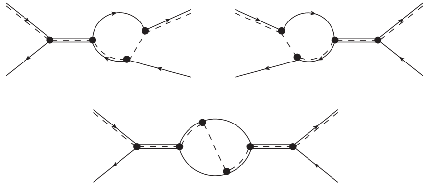
Figure 14: The pion-exchange diagrams for $D^{*0}\bar{D}^{0}\to D^{*0}\bar{D}^{0}$ consist of the 1-loop diagrams A1 and A2 and the 2-loop diagram A3. The absence of arrows on the charm-mesons lines in the loop for the diagram A3 implies a sum over the two possible directions of the arrows.

There are three NLO pion-exchange diagrams for $D^{*0}\bar{D}^{0}\to D^{*0}\bar{D}^{0}$. They are shown in Fig. 14 and are labelled A1, A2, and A3.

The amplitudes for the 1-loop diagrams A1 and A2 in Fig. 14 are tensors in the indices $i$ and $j$ that depend on the relative momenta $\bm{p}^{\prime}$ and $\bm{p}$, respectively. The amplitude for the diagram A2 is

$$\mathcal{T}_{\mathrm{A2}}^{ij}(E,\bm{p}) = \frac{r\pi g_{\pi}^{2}/\mu}{(d-1)\sqrt{1-r}\,p^{2}}\mathcal{A}(E)\Big{\{}\big{[}(\Delta(E,p)-2rp^{2})L_{0}(E,p)$$ (142)

$$\hskip 142.26378pt-(\Delta(E,p)^{2}-8r\mu E_{*}p^{2})L_{1}(E,p)$$

$$\hskip 142.26378pt-(\Delta(E,p)-2p^{2})J_{1}(E)\big{]}(\delta^{ij}-p^{i}p^{j}/p^{2})$$

$$\hskip 28.45274pt-(d-1)\big{[}\Delta(E,p)L_{0}(E,p)-\Delta(E,p)(\Delta(E,p)-2rp^{2})L_{1}(E,p)$$

$$\hskip 142.26378pt-(\Delta(E,p)+2(1-r)p^{2})J_{1}(E)\big{]}p^{i}p^{j}/p^{2}\Big{\}},$$

where $r=\mu_{\pi}/\mu$ and $\Delta$ is a linear function of $E$ and $p^{2}$:

$$\Delta(E,p)=2\mu E_{*}-2(1-r)\mu E+p^{2}.$$ (143)

The S-wave contribution of the diagram can be obtained by averaging over the directions of $\bm{p}$ in $d$ spatial dimensions:

$$\Big{\langle}\mathcal{T}^{ij}_{\mathrm{A2}}(E,\bm{p})\Big{\rangle}_{\hat{\bm{p}}} = \frac{2\pi rg_{\pi}^{2}/\mu}{d\sqrt{1-r}}\big{[}-r\,L_{0}(E,p)-r\,\big{(}\Delta(E,p)-4\mu E_{*}\big{)}L_{1}(E,p)$$ (144)

$$\hskip 56.9055pt+(2-r)J_{1}(E)\big{]}\mathcal{A}(E)\,\delta^{ij}.$$

The S-wave contribution $\langle\mathcal{T}^{ij}_{\mathrm{A1}}(E,\bm{p}^{\prime})\rangle_{\hat{\bm{p}}^{\prime}}$ to the diagram A1 can be obtained by replacing $p$ in Eq. (144) by $p^{\prime}$. In Ref. Braaten:2015tga , it was stated incorrectly that the $p^{i}p^{j}/p^{2}$ terms in Eq. (142) cancel in the limit $\bm{p}\to 0$. They do however cancel in the limit $p\to 0$ after averaging over the directions of $\bm{p}$.

The 2-loop diagram A3 in Fig. 14 is the sum of a diagram with a $D^{*0}\bar{D}^{0}$ loop and a diagram with a $D^{0}\bar{D}^{*0}$ loop. The amplitude for this diagram is

$$\mathcal{T}^{ij}_{\mathrm{A3}}(E)=-\frac{8\pi^{2}rg_{\pi}^{2}/\mu}{d\sqrt{1-r}}\big{[}2K_{110}(E)-2\mu(2E_{*}-rE)K_{111}(E)-(2-r)J_{1}(E)^{2}\big{]}\mathcal{A}^{2}(E)\,\delta^{ij}.~{}~{}~{}$$ (145)

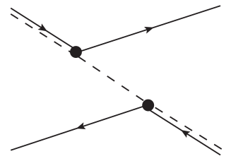
Figure 15: The pion-exchange tree diagram for $D^{*0}\bar{D}^{0}\to D^{0}\bar{D}^{*0}$, which is labelled $\pi$. There are also three loop diagrams that can be obtained from those in Fig. 14 by changing the directions of some of the arrows.

For each of the pion-exchange diagrams for $D^{*0}\bar{D}^{0}\to D^{*0}\bar{D}^{0}$ in Fig. 14, there is an analogous diagram for $D^{*0}\bar{D}^{0}\to D^{0}\bar{D}^{*0}$, $D^{0}\bar{D}^{*0}\to D^{*0}\bar{D}^{0}$, and $D^{0}\bar{D}^{*0}\to D^{0}\bar{D}^{*0}$. For $D^{*0}\bar{D}^{0}\to D^{0}\bar{D}^{*0}$ and $D^{0}\bar{D}^{*0}\to D^{*0}\bar{D}^{0}$, there is also a tree diagram. The tree diagram for $D^{*0}\bar{D}^{0}\to D^{0}\bar{D}^{*0}$ is shown in Fig. 15, and it is labelled $\pi$. The transition tensor for this diagram depends on the relative momenta $\bm{p}$ and $\bm{p}^{\prime}$:

$$\mathcal{T}_{\pi}^{ij}(E,\bm{p},\bm{p}^{\prime})=-\frac{g_{\pi}^{2}/\mu^{2}}{E-(p^{2}+{p^{\prime}}^{2})/(2M)-(\bm{p}+\bm{p}^{\prime})^{2}/(2m)+i\epsilon}$$

$$\times\left(\frac{M}{M+m}\bm{p}+\bm{p}^{\prime}\right)^{i}\left(\frac{M}{M+m}\bm{p}^{\prime}+\bm{p}\right)^{j}.$$ (146)

This diagram vanishes in the zero-momentum limit $\bm{p},\bm{p}^{\prime}\to 0$ with $E$ fixed. Since this diagrams does not have any UV divergences, the S-wave contribution of the diagram can be obtained by averaging over the directions of $\bm{p}$ and $\bm{p}^{\prime}$ in 3 spatial dimensions:

$$\Big{\langle}\mathcal{T}^{ij}_{\pi}(E,\bm{p},\bm{p}^{\prime})\Big{\rangle}_{\hat{\bm{p}},\hat{\bm{p}}^{\prime}} = -\frac{rg_{\pi}^{2}/\mu}{3\sqrt{1-r}}\Bigg{(}\frac{r[2(2-r)\mu E-p^{2}-p^{\prime 2}]}{4\sqrt{1-r}\,p\,p^{\prime}}$$ (147)

$$\hskip 28.45274pt\times\log\frac{2r\mu E-p^{2}-p^{\prime 2}+2\sqrt{1-r}\,p\,p^{\prime}}{2r\mu E-p^{2}-p^{\prime 2}-2\sqrt{1-r}\,p\,p^{\prime}}-(2-r)\Bigg{)}\delta^{ij}.$$

B.3 $\bm{D^{*}}$ propagator correction diagrams

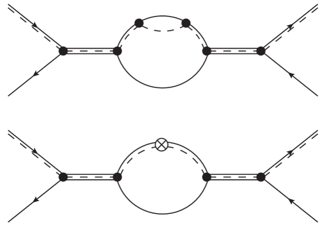
Figure 16: The $D^{*}$ propagator correction diagrams for $D^{*0}\bar{D}^{0}\to D^{*0}\bar{D}^{0}$ consist of the 2-loop diagram B1 with a $D^{*}$ self-energy subdiagram and the 1-loop diagram B2 with a $D^{*}$ self-energy counterterm.

The two NLO diagrams involving $D^{*}$ propagator corrections are shown in Fig. 16 and are labelled B1 and B2. The diagram B1, which has a $D^{*}$ self-energy subdiagram inserted into the $D^{*}$ propagator, can be reduced to

$$\mathcal{T}^{ij}_{\mathrm{B1}}(E)=-\frac{16\pi^{2}rg_{\pi}^{2}/\mu}{d}\big{[}K_{110}(E)-2\mu E_{*}K_{120}(E)\big{]}\mathcal{A}^{2}(E)\,\delta^{ij}.$$ (148)

The diagram B2, which has a $D^{*}$ propagator counterterm inserted into the $D^{*}$ propagator, can be reduced to

$$\mathcal{T}^{ij}_{\mathrm{B2}}(E)=-\frac{8\pi^{2}r^{2}g_{\pi}^{2}/\mu}{d}I_{1}(E_{*})\big{[}4\mu E_{*}J_{2}(E)-dJ_{1}(E)\big{]}\mathcal{A}^{2}(E)\,\delta^{ij}.$$ (149)

B.4 $\bm{\nabla^{2}}$ vertex diagrams

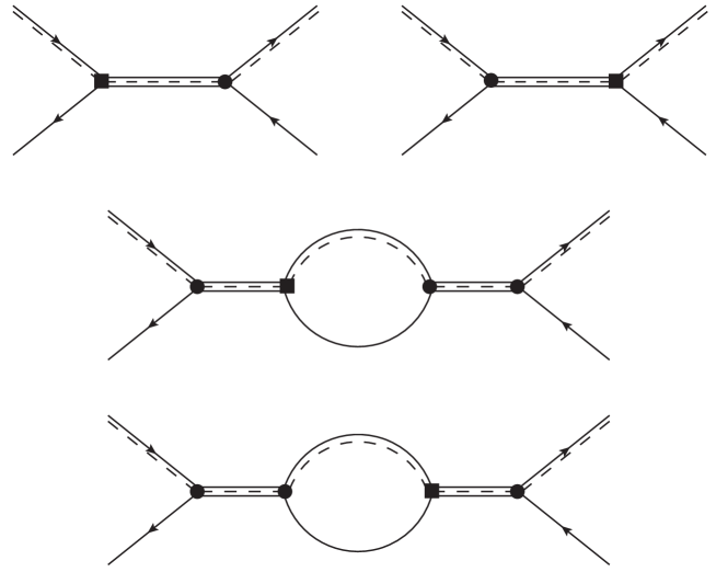
Figure 17: The $\nabla^{2}$ vertex diagrams for $D^{*0}\bar{D}^{0}\to D^{*0}\bar{D}^{0}$ consist of two tree diagrams C1 and C2 and two 1-loop diagrams C3 and C4.

The four NLO diagrams with a $\nabla^{2}$ vertex are shown in Fig. 17 and are labelled C1, C2, C3, and C4. The diagram C1 in which the incoming charm mesons interact through a $\nabla^{2}$ vertex is

$$\mathcal{T}_{\mathrm{C1}}^{ij}(E,p)=\frac{\pi C_{2}}{2\mu C_{0}}\mathcal{A}(E)\,p^{2}\,\delta^{ij}.$$ (150)

The diagram C2 in which the outgoing charm mesons interact through a $\nabla^{2}$ vertex is obtained by replacing $p^{2}$ by ${p^{\prime}}^{2}$. The diagram C3 is

$$\mathcal{T}_{\mathrm{C3}}^{ij}(E)=\frac{4\pi^{2}C_{2}}{C_{0}}(E-E_{*})J_{1}(E)\,\mathcal{A}^{2}(E)\,\delta^{ij}.$$ (151)

The expression for the diagram C4 is the same. The sum of the four diagrams is

$$\mathcal{T}_{\mathrm{C}}^{ij}(E,p,p^{\prime})=\frac{\pi C_{2}}{2\mu C_{0}}\Big{[}(p^{2}+{p^{\prime}}^{2})\mathcal{A}(E)+16\pi\mu(E-E_{*})J_{1}(E)\mathcal{A}^{2}(E)\Big{]}\delta^{ij}.$$ (152)

With the Feynman rules in Ref. Braaten:2015tga , the $\nabla^{2}$ vertices are $2\to 2$ vertices. There are four $\nabla^{2}$ vertex diagrams: the $\nabla^{2}$ vertex, two 1-loop diagrams with a single factor of $\mathcal{A}(E)$, and a 2-loop diagram with two factors of $\mathcal{A}(E)$. The identity in Eq. (47) can be used to show the sum of the four diagrams is the same as that in Eq. (152).

B.5 Pair-propagator counterterm diagram

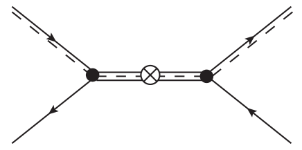
Figure 18: The pair propagator counterterm diagram for $D^{*0}\bar{D}^{0}\to D^{*0}\bar{D}^{0}$, which is labelled D.

The NLO diagram with a pair-propagator counterterm is shown in Fig. 18. The expression for the diagram is

$$\mathcal{T}^{ij}_{\mathrm{D}}(E)=-\frac{2\pi^{2}}{\mu^{2}C_{0}^{2}}\,\big{[}\delta C_{0}+D_{0}\,(E-E_{*})\big{]}\,\mathcal{A}^{2}(E)\delta^{ij}.$$ (153)

With the Feynman rules in Ref. Braaten:2015tga , there is a $2\to 2$ vertex counterterm. There are four NLO diagrams with a counterterm vertex: the vertex counterterm, two 1-loop diagrams with a single factor of $\mathcal{A}(E)$, and a 2-loop diagram with two factors of $\mathcal{A}(E)$. The identity in Eq. (47) can be used to show the sum of the four diagrams is equal to that in Eq. (153).

References

- (1) A. Ali, J.S. Lange and S. Stone, Exotics: Heavy Pentaquarks and Tetraquarks, Prog. Part. Nucl. Phys. 97, 123 (2017) [arXiv:1706.00610].
- (2) S.L. Olsen, T. Skwarnicki and D. Zieminska, Nonstandard heavy mesons and baryons: Experimental evidence, Rev. Mod. Phys. 90, 015003 (2018) [arXiv:1708.04012].
- (3) M. Karliner, J.L. Rosner and T. Skwarnicki, Multiquark States, Ann. Rev. Nucl. Part. Sci. 68, 17 (2018) [arXiv:1711.10626].
- (4) N. Brambilla, S. Eidelman, C. Hanhart, A. Nefediev, C. P. Shen, C.E. Thomas, A. Vairo and C.Z. Yuan, The states: experimental and theoretical status and perspectives, Phys. Rept. 873, 1-154 (2020) [arXiv:1907.07583].
- (5) S.K. Choi et al. [Belle], Observation of a narrow charmonium-like state in exclusive decays, Phys. Rev. Lett. 91, 262001 (2003) [arXiv:hep-ex/0309032].
- (6) R. Aaij et al. [LHCb], Determination of the meson quantum numbers, Phys. Rev. Lett. 110, 222001 (2013) [arXiv:1302.6269].
- (7) R. Aaij et al. [LHCb], Study of the lineshape of the state, [arXiv:2005.13419 [hep-ex]].
- (8) R. Aaij et al. [LHCb], Study of the and states in decays, JHEP 08, 123 (2020) [arXiv:2005.13422].
- (9) E. Braaten and M. Kusunoki, Low-energy universality and the new charmonium resonance at 3870-MeV, Phys. Rev. D 69, 074005 (2004) [arXiv:hep-ph/0311147].
- (10) E. Braaten and H. W. Hammer, Universality in few-body systems with large scattering length, Phys. Rept. 428, 259-390 (2006) [arXiv:cond-mat/0410417].
- (11) S. Fleming, M. Kusunoki, T. Mehen and U. van Kolck, Pion interactions in the , Phys. Rev. D 76, 034006 (2007) [arXiv:hep-ph/0703168].
- (12) E. Braaten, Galilean-invariant effective field theory for the , Phys. Rev. D 91, 114007 (2015) [arXiv:1503.04791].
- (13) C.R. Hagen, Scale and conformal transformations in galilean-covariant field theory, Phys. Rev. D 5, 377-388 (1972).
- (14) G. Rosen, Galilean invariance and the general covariance of nonrelativistic laws, Am. J. Phys. 40, 683-687 (1972).
- (15) M. Jansen, H.W. Hammer and Y. Jia, Light quark mass dependence of the X(3872) in an effective field theory, Phys. Rev. D 89, 014033 (2014) [arXiv:1310.6937].
- (16) L. Dai, F.K. Guo and T. Mehen, Revisiting in an effective field theory for the , Phys. Rev. D 101, 054024 (2020) [arXiv:1912.04317 ].
- (17) X. Kong and F. Ravndal, Coulomb effects in low-energy proton proton scattering, Nucl. Phys. A 665, 137-163 (2000) [arXiv:hep-ph/9903523].
- (18) E. Braaten, E. Johnson and H. Zhang, Zero-range effective field theory for resonant wino dark matter. Part II. Coulomb resummation, JHEP 02, 150 (2018) [arXiv:1708.07155].
- (19) E. Braaten, H. W. Hammer and T. Mehen, Scattering of an Ultrasoft Pion and the , Phys. Rev. D 82, 034018 (2010) [arXiv:1005.1688].
- (20) D.L. Canham, H.-W. Hammer and R.P. Springer, On the scattering of and mesons off the , Phys. Rev. D 80, 014009 (2009) [arXiv:0906.1263].
- (21) S. Dubynskiy and M.B. Voloshin, near the threshold, Phys. Rev. D 74, 094017 (2006) [hep-ph/0609302].
- (22) E. Braaten, L.-P. He and K. Ingles, Production of Accompanied by a Pion in Meson Decay, Phys. Rev. D 100, 074028 (2019) [arXiv:1902.03259].
- (23) E. Braaten, L.-P. He and K. Ingles, Production of Accompanied by a Soft Pion at Hadron Colliders, Phys. Rev. D 100, 094006 (2019) [arXiv:1903.04355].
- (24) F.K. Guo, Novel method for precisely measuring the mass, Phys. Rev. Lett. 122, 202002 (2019) [arXiv:1902.11221].
- (25) E. Braaten, L. P. He and K. Ingles, Triangle Singularity in the Production of and a Photon in Annihilation, Phys. Rev. D 100, 031501 (2019) [arXiv:1904.12915].
- (26) E. Braaten, L.P. He, K. Ingles and J. Jiang, Charm-meson triangle singularity in annihilation into , Phys. Rev. D 101, 096020 (2020) [arXiv:2004.12841].
- (27) S. Sakai, E. Oset and F.K. Guo, Triangle singularity in the reaction and sensitivity to the mass, Phys. Rev. D 101, 054030 (2020) [arXiv:2002.03160].
- (28) R. Molina and E. Oset, Triangle singularity in and the X(3872) mass, Eur. Phys. J. C 80, 451 (2020) [arXiv:2002.12821].
- (29) S. Sakai, H.J. Jing and F.K. Guo, Possible precise measurements of the mass with the and reactions, [arXiv:2008.10829].