Detecting the skewness of data from the five-number summary and its application in meta-analysis

Abstract

For clinical studies with continuous outcomes, when the data are potentially skewed, researchers may choose to report the whole or part of the five-number summary (the sample median, the first and third quartiles, and the minimum and maximum values) rather than the sample mean and standard deviation. In the recent literature, it is often suggested to transform the five-number summary back to the sample mean and standard deviation, which can be subsequently used in a meta-analysis. However, if a study contains skewed data, this transformation and hence the conclusions from the meta-analysis are unreliable. Therefore, we introduce a novel method for detecting the skewness of data using only the five-number summary and the sample size, and meanwhile propose a new flow chart to handle the skewed studies in a different manner. We further show by simulations that our skewness tests are able to control the type I error rates and provide good statistical power, followed by a simulated meta-analysis and a real data example that illustrate the usefulness of our new method in meta-analysis and evidence-based medicine.

$Key\ words$: Evidence-based medicine, Five-number summary, Flow chart, Meta-analysis, Skewness test

1 Introduction

Meta-analysis is an important tool to synthesize the research findings from multiple studies for decision making. To conduct a meta-analysis, the summary statistics are routinely collected from each individual study, and in particular for continuous outcomes, they consist of the sample mean and standard deviation (SD). In many other studies, if the data are skewed, researchers may instead report the whole or part of the five-number summary $\{a,q_{1},m,q_{3},b\}$, where $a$ is the minimum value, $q_{1}$ is the first quartile, $m$ is the sample median, $q_{3}$ is the third quartile, and $b$ is the maximum value. More specifically, by letting $n$ be the size of the data, the three common scenarios for reporting the five-number summary include

$$\mathcal{S}_{1} =\{a,m,b;n\},$$

$$\mathcal{S}_{2} =\{q_{1},m,q_{3};n\},$$

$$\mathcal{S}_{3} =\{a,q_{1},m,q_{3},b;n\}.$$

In practice, however, few existing methods in meta-analysis are able to pool together the studies with the sample mean and SD and the studies with the five-number summary.

To overcome this problem, there are two common approaches in the literature. The first approach is to exclude the studies with the five-number summary from meta-analysis by labeling them as “studies with insufficient data”. This approach was, in fact, quite popular in the early years. Nevertheless, by doing so, valuable information may be excluded so that the final meta-analytical result can be less reliable or even misleading, especially when a large proportion of studies are reported with the five-number summary. In contrast, the second approach is to apply the recently developed methods [1, 2, 3, 4] that convert the five-number summary back to the sample mean and SD, and then include them in the subsequent meta-analysis. It is noteworthy that these transformation methods have been attracting increasing attention in meta-analysis and evidence-based practice. More recently, our transformation methods in Wan et al.[2], Luo et al.[3] and Shi et al.[4], have also been adopted as the default methods for handling the five-number summary in R packages $meta$ [5, 6] and $metafor$ [7, 8], and the three papers have received 4853, 1212 and 154 citations, respectively, in Google Scholar as of 03 March 2023.

Despite the popularity of the second approach, it is also noteworthy that the aforementioned transformation methods are all built on the basis of the normality assumption for the underlying data. When the data are skewed, however, these normal-based methods may no longer be able to provide reliable estimates for the true sample mean and SD. For more details, see the motivating examples in Section 2. As a consequence, if we do not handle such skewed studies in a proper way, it may result in misleading or even completely wrong conclusions in the subsequent meta-analysis [9, 10].

This motivates us to perform the normality test for the data first, whose result will guide the subsequent steps as presented in the flow chart of Figure 1.

For the normality test, there is a large body of literature on mainly two different types of tests, (1) the graphical methods [11], and (2) the quantitative normality test [12, 13, 14, 15, 16]. Nevertheless, we note that most existing normality tests require the complete data set so that they are not applicable when the data include only the whole or part of the five-number summary. For this issue, Altman and Bland[17] also discussed in their short note as follows: “When authors present data in the form of a histogram or scatter diagram then readers can see at a glance whether the distributional assumption is met. If, however, only summary statistics are presented—as is often the case—this is much more difficult.”.

To summarize, when only the five-number summary is available, there is currently no method available for testing whether the underlying data follow a normal distribution. In this paper, we propose a skewness test based on the five-number summary together with the sample size. Further by the symmetry of the normal distribution, if the skewness test shows that the data are significantly skewed, then equivalently we can also conclude that the data are not normally distributed. For these skewed studies, we provide practitioners with three options in Figure 1. On the contrary, if the skewness test is not rejected, then we follow the common practice that assumes the reported data to be normal. Following the above procedure, we will have the capacity to rule out the very skewed studies so that the final meta-analysis can be conducted more reliably than the existing methods in the literature. Finally, due to the limited information available from the five-number summary, we believe that our proposed flow chart in Figure 1 also provides a reasonable solution for conducting meta-analysis that handles both normal and skewed studies, and we also expect that it may have potential to be widely adopted in meta-analysis and evidence-based practice.

Figure 1: A flow chart for conducting meta-analysis when some studies from systematic review are reported with the whole or part of the five-number summary.

2 Motivating examples

To start with, we first present a simulation study to evaluate the performance of the existing transformation methods [2, 3, 4] when the underlying distribution is skewed away from normality. Specifically, we consider four normal-related distributions [18] as follows: (i) the skew-normal distribution with parameters $\delta=0$, $\omega=1$ and $\alpha=-10$, (ii) the half-normal distribution with parameters $\mu=0$ and $\sigma^{2}=1$, (iii) the log-normal distribution with parameters $\mu=0$ and $\sigma^{2}=1$, and (iv) the mixture-normal distribution that takes the values from $N(-2,1)$ with probability 0.3 and from $N(2,1)$ with probability 0.7. To visualize the skewness of the distributions, the probability density functions of the four distributions are also plotted in Figure 2. It is evident that they are all skewed away, more or less, from the normal distribution.

Table 1: The true and estimated averages (standard errors) of the sample mean and SD under scenario $\mathcal{S}_{1}$ for the four normal-related distributions.

Distribution	Sample mean		Sample SD
	True value	Estimated value [3]	True value	Estimated value [2]
Skew-normal	-0.79 (0.04)	-0.73 (0.05)	0.61 (0.04)	0.57 (0.07)
Half-normal	0.80 (0.04)	0.73 (0.05)	0.60 (0.04)	0.54 (0.07)
Log-normal	1.65 (0.16)	1.53 (0.32)	2.09 (0.56)	3.10 (1.57)
Mixture-normal	0.80 (0.15)	1.34 (0.14)	2.09 (0.08)	1.63 (0.11)

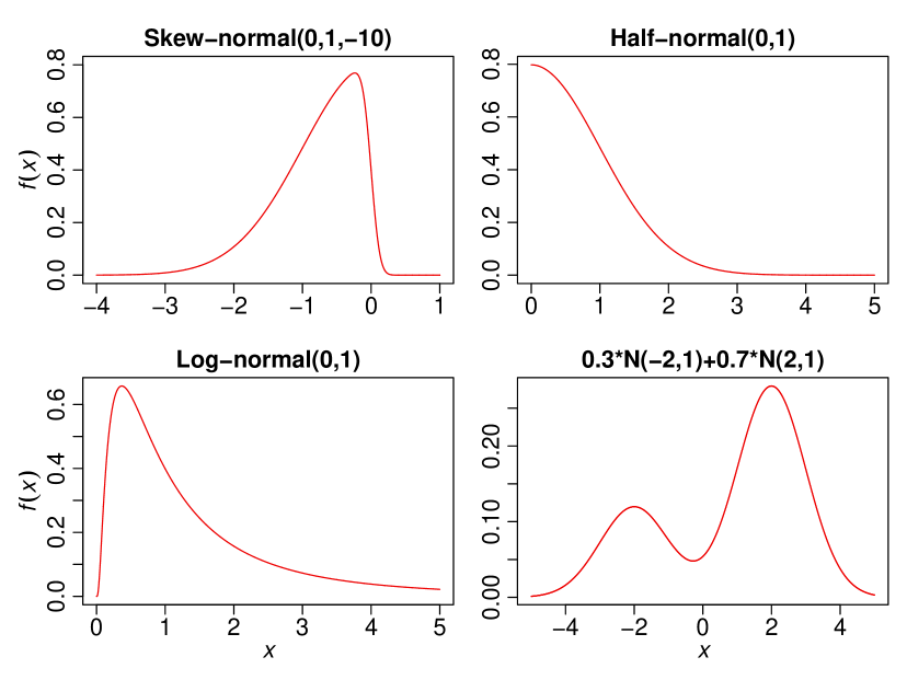
Figure 2: Probability density functions of the four normal-related distributions including Skew-normal(0, 1,-10), Half-normal(0, 1), Log-normal(0, 1), and 0.3*$N$(-2, 1)+0.7*$N$(2, 1).

Next, for each distribution, a sample of size 200 is randomly generated. With the complete sample, we can readily compute the sample mean and SD, and also collect the sample median, the minimum and maximum values. Now to evaluate the normal-based methods for transformation, we further apply Luo et al.[3] to estimate the sample mean and Wan et al.[2] to estimate the sample SD under scenario $\mathcal{S}_{1}$. With 100,000 simulations, we report the averages (standard errors) of the estimated sample mean and SD, together with the averages (standard errors) of the true sample mean and SD, in Table 1. From the simulated results, it is evident that the converted sample mean and SD using the normal-based methods are less accurate for all four skewed distributions. In particular, we note that the sample SD is significantly overestimated for $\text{Log-normal}(0,1)$, and the sample mean is significantly overestimated for the mixture-normal distribution.

Table 2: The summary statistics, sample median (IQR) [sample size], of the four studies in the meta-analysis from Wu and Yang.[19]

Study	Nonsurvivors	Survivors
Chen et al.[20]	28 (18-47) [113]	20 (14.8-32) [161]
Du et al.[21]	27 (20-37) [21]	22 (14-40.5) [158]
Wang et al.[22]	24 (19-49) [65]	28 (17-43) [274]
Zhou et al.[23]	40 (24-51) [54]	27 (15-40) [135]

Our second example is a real study that investigates the impact of COVID-19 on liver dysfunction by a meta-analysis [19]. The serum alanine aminotransferase (ALT), as an important index to measure the dysfunction of the liver, was a primary outcome of interest. By setting the nonsurvivors and survivors as the case and control groups, the liver dysfunction can be compared by the ALT level difference between the two groups. Four clinical studies that paid attention to the ALT level were included in the meta-analysis with the sample median and the interquartile range (IQR) being reported in Table 2. The potential skewness of the underlying data can be observed by comparing the distances between the sample median and the first quartile or the third quartile. Taking the nonsurvivors group in Wang et al.[22] as an example, the distance between the sample median to the third quartile $(49-24=25)$ is five times as that between the sample median to the first quartile $(24-19=5)$, indicating a large degree of skewness. For more details, see Section 5 where the skewed groups with statistical significance are all identified. Such skewed data, if not properly handled, may lead to unreliable or even misleading conclusions for decision making in evidence-based practice.

3 Detecting the skewness from the five-number summary

As sketched in Figure 1, to handle the clinical studies reported with the whole or part of the five-number summary, the first and foremost thing is to detect whether or not the data follow a normal distribution. When the normality assumption does not hold, the reported data from the clinical study were often skewed, which is, in fact, one main reason why researchers had preferred to report the five-number summary. In this section, we will formulate the null and alternative hypotheses for detecting the skewness of data under the three common scenarios, and then construct their test statistics, as well as derive their null distributions and the critical regions.

Let $X_{1},X_{2},\ldots,X_{n}$ be a random sample of size $n$ from the normal distribution with mean $\mu$ and variance $\sigma^{2}$, and $X_{(1)}\leq X_{(2)}\leq\cdots\leq X_{(n)}$ be the corresponding order statistics. Then, for simplicity, by letting $Q$ be a positive integer, the five-number summary can be represented as $a=X_{(1)}$, $q_{1}=X_{(Q+1)}$, $m=X_{(2Q+1)}$, $q_{3}=X_{(3Q+1)}$ and $b=X_{(n)}$. Let also $X_{i}=\mu+\sigma Z_{i}$ for $i=1,\ldots,n$, or equivalently,

$$X_{(i)}=\mu+\sigma Z_{(i)},$$ (1)

where $Z_{1},Z_{2},\ldots,Z_{n}$ are independent random variables from the standard normal distribution, and $Z_{(1)}\leq Z_{(2)}\leq\cdots\leq Z_{(n)}$ are the order statistics. Lastly, when $Q$ is not an integer, we suggest to apply the interpolation method to calculate the critical values with details in Appendix B.

3.1 Detecting the skewness under scenario $\mathcal{S}_{1}=\{a,m,b;n\}$

We first consider scenario $\mathcal{S}_{1}$ where the minimum, median, and maximum values are available together with the sample size. When the data are normally distributed, we expect that the distance between $a$ and $m$ should be not far away from the distance between $m$ and $b$. More specifically, by Lemma 1 in Appendix A and the facts that $E(m-a)=\sigma E(Z_{(2Q+1)}-Z_{(1)})$ and $E(b-m)=\sigma E(Z_{(n)}-Z_{(2Q+1)})$, we have $E(m-a)=E(b-m)$. In view of this, we define $\theta_{1}=E(b-m)-E(m-a)=E(a+b-2m)$ as the level of skewness for the underlying distribution of the data. Then to detect the skewness of data, we propose to consider the following hypotheses:

$$H_{0}:\theta_{1}=0\quad\quad\text{versus}\quad\quad H_{1}:\theta_{1}\neq 0.$$

If the null hypothesis is rejected, we then conclude that the data are significantly skewed, and moreover by the flow chart in Figure 1, we recommend practitioners to take the proper choice from the three options for skewed studies.

Now to test whether $\theta_{1}=0$ under scenario $\mathcal{S}_{1}$, by the Wald test [24], we consider the test statistic as

$$W_{1}=\dfrac{a+b-2m}{{\rm SE}(a+b-2m)},$$

where ${\rm SE}(a+b-2m)$ denotes the standard error of $a+b-2m$ under the null hypothesis. By formula (1), we can rewrite ${\rm SE}(a+b-2m)=\sigma\delta_{1}(n)$, where $\sigma$ is the SD of the normal distribution and $\delta_{1}(n)={\rm SE}(Z_{(1)}+Z_{(n)}-2Z_{(2Q+1)})$. Next, for the unknown $\sigma$, we consider to estimate it by the method in Wan et al.[2] Specifically, we have $\hat{\sigma}_{1}=(b-a)/\xi(n)$, where $\xi(n)=2\Phi^{-1}[(n-0.375)/(n+0.25)]$ and $\Phi^{-1}$ is the quantile function of the standard normal distribution. Finally, by noting that $\delta_{1}(n)$ and $\xi(n)$ are fixed values for any given $n$, we remove them from the Wald statistic and that yields our final test statistic as

$$T_{1}=\dfrac{a+b-2m}{b-a}.$$ (2)

In the special case when $a=b$, all the observations are tied so that a test for skewness may not be possible. To further derive the null distribution of the test statistic $T_{1}$, we consider two different approaches where the first one is to derive the asymptotic null distribution when $n$ tends to infinity, and the second one is to derive the exact null distribution for any fixed $n$.

For the first approach, noting that $T_{1}$ involves the extreme order statistics, the asymptotic null distribution will not follow a normal distribution as that for a classical Wald statistic [25]. To further clarify it, when $n$ is large, the extreme order statistics will tend to be less stable than the intermediate order statistics and hence provide a slower convergence rate toward the asymptotic distribution for the given test statistic. Specifically by Theorem 1 in Appendix A, under the null hypothesis, we show that

$$\sqrt{2\ln(n)}\xi(n)T_{1}\overset{D}{\longrightarrow}{\rm Logistic}(0,1),\quad{\rm as}\ n\rightarrow\infty,$$ (3)

where $\overset{D}{\longrightarrow}$ denotes the convergence in distribution, and Logistic$(0,1)$ represents the logistic distribution with location parameter $\mu=0$ and scale parameter $s=1$. Noting also that the asymptotic null distribution is symmetric about zero, we can specify the critical region of size $\alpha$ as $\{t_{1,{\rm obs}}:|t_{1,{\rm obs}}|>l_{\alpha/2}/(\sqrt{2\ln(n)}\xi(n))\},$ where $t_{1,{\rm obs}}$ is the observed value of $T_{1}$ and $l_{\alpha/2}$ is the upper $\alpha/2$ quantile of ${\rm Logistic}(0,1)$. Despite of the elegant analytical results, the asymptotic test by (3) will have a serious limitation that the convergence rate is relatively slow at the order of $\sqrt{2\ln(n)}\xi(n)$. Moreover, the simulation results in Section 4 will show that the asymptotic null distribution fails to control the type I error rates for some small sample sizes.

To improve the detection accuracy, our second approach is to derive the exact null distribution of $T_{1}$ for any fixed $n$. By (1) and (2), we can represent the test statistic as

$$T_{1}=\frac{Z_{(1)}+Z_{(n)}-2Z_{(2Q+1)}}{Z_{(n)}-Z_{(1)}}.$$ (4)

Since the right-hand side of (4) is purely a function of the order statistics of the standard normal distribution, the null distribution of $T_{1}$ will be free of the parameters $\mu$ and $\sigma^{2}$. Moreover, we have derived the sampling distribution of $T_{1}$ under the null hypothesis in Theorem 2 of Appendix A. Further by the symmetry of the null distribution, the critical region of size $\alpha$ can be specified as

$$\{t_{1,{\rm obs}}:|t_{1,{\rm obs}}|>c_{1,\alpha/2}(n)\},$$

where $c_{1,\alpha/2}(n)$ is the upper $\alpha/2$ quantile of the null distribution of $T_{1}$ for the sample size $n$. If the test is rejected based on the reported summary statistics, we then conclude that the data from the study are significantly skewed.

From the practical point of view, however, the null distribution of $T_{1}$ has a complicated form so that the true values of $c_{1,\alpha/2}(n)$ may not be readily known. To help practitioners and also promote the new test, by the R software we have provided the numerical values of $c_{1,\alpha/2}(n)$ for $n$ up to 401 with $\alpha=0.05$ in Table 5 of Appendix B. Moreover, an approximate formula $c_{1,0.025}(n)\approx 1/\ln(n+9)+2.5/(n+1)$ is also given for easy implementation of the critical values for any given sample size. It is evident, as shown in Figure 8 of Appendix B, that the approximation is quite accurate so that it can serve well as a “rule of thumb” for practical use. Specifically by the rule of thumb, the skewness test can be performed by first computing the absolute value of the observed test statistic, and then examining whether it is larger or smaller than the approximated threshold value at $1/\ln(n+9)+2.5/(n+1)$.

3.2 Detecting the skewness under scenario $\mathcal{S}_{2}=\{q_{1},m,q_{3};n\}$

Under scenario $\mathcal{S}_{2}$, the reported summary data include the first quartile, the median and the third quartile together with the sample size. When the data are normally distributed, we expect that the distance between $q_{1}$ and $m$ should be close to the distance between $m$ and $q_{3}$. Specifically, by Lemma 1 in Appendix A and the facts that $E(m-q_{1})=\sigma E(Z_{(2Q+1)}-Z_{(Q+1)})$ and $E(q_{3}-m)=\sigma E(Z_{(3Q+1)}-Z_{(2Q+1)})$, we have $E(m-q_{1})=E(q_{3}-m)$. We then define $\theta_{2}=E(q_{3}-m)-E(m-q_{1})=E(q_{1}+q_{3}-2m)$ as the level of skewness for the underlying distribution of the data. Finally for detecting the skewness of data, we consider the following hypotheses:

$$H_{0}:\theta_{2}=0\quad\quad\text{versus}\quad\quad H_{1}:\theta_{2}\neq 0.$$

If the null hypothesis is rejected, we conclude that the underlying distribution of the data is significantly skewed.

Following the same spirit as under scenario $\mathcal{S}_{1}$, for the above hypotheses we consider the test statistic

$$T_{2}=\frac{q_{1}+q_{3}-2m}{q_{3}-q_{1}},$$ (5)

where $q_{3}>q_{1}$. Note that $T_{2}$ has also been adopted by Groeneveld and Meeden[26] as a measure of skewness. Moreover, unlike the test statistic $T_{1}$ that involves the extreme order statistics, the asymptotic normality of $T_{2}$ can be readily established. Specifically in Theorem 3 of Appendix A, we have shown that

$$0.74\sqrt{n}T_{2}\overset{D}{\longrightarrow}N(0,1),\quad{\rm as}\ n\rightarrow\infty.$$ (6)

Further by (6), the critical region of size $\alpha$ can be approximately as $\{t_{2,{\rm obs}}:|t_{2,{\rm obs}}|>z_{\alpha/2}/(0.74\sqrt{n})\},$ where $t_{2,{\rm obs}}$ is the observed value of $T_{2}$ and $z_{\alpha/2}$ is the upper $\alpha/2$ quantile of the standard normal distribution.

Nevertheless, given that the asymptotic critical values can be quite large especially for small sample sizes, the above asymptotic test may not provide an adequate power for detecting the skewness. To further improve the detection accuracy, we have also derived the exact null distribution of $T_{2}$ in Theorem 4 of Appendix A for any fixed $n$. Noting also that the null distribution of $T_{2}$ is symmetric about zero, we can specify the exact critical region of size $\alpha$ as follows:

$$\{t_{2,{\rm obs}}:|t_{2,{\rm obs}}|>c_{2,\alpha/2}(n)\},$$

where $c_{2,\alpha/2}(n)$ is the upper $\alpha/2$ quantile of the null distribution of $T_{2}$ for the sample size $n$. If the observed value of $T_{2}$ falls in the critical region, it is concluded that the data are significantly skewed away from normality.

Finally, as that for scenario $\mathcal{S}_{1}$, we note that obtaining the critical values by Theorem 4 in Appendix A is rather complicated and not readily accessible. Thus to help practitioners, we have computed the numerical values of $c_{2,\alpha/2}(n)$ for $\alpha=0.05$ with $n$ up to 401 in Table 6 of Appendix B. For ease of implementation, an approximate formula for the critical values is also provided as $c_{2,0.025}\approx 2.65/\sqrt{n}-6/n^{2}$, with its approximation accuracy reported in Figure 8 of Appendix B. Consequently, it also provides a convenient way for practitioners to detect the skewness of data by hand.

3.3 Detecting the skewness under scenario $\mathcal{S}_{3}=\{a,q_{1},m,q_{3},b;n\}$

In this section, we consider the detection of skewness under scenario $\mathcal{S}_{3}$ when the five-number summary is fully available together with the sample size. For normal data, we have $E(m-a)=E(b-m)$ and $E(m-q_{1})=E(q_{3}-m)$, or equivalently, $\theta_{1}=E(a+b-2m)=0$ and $\theta_{2}=E(q_{1}+q_{3}-2m)=0$. Noting also that the summary data under scenario $\mathcal{S}_{3}$ is the union of those under scenarios $\mathcal{S}_{1}$ and $\mathcal{S}_{2}$, we consider the following joint hypothesis for detecting the skewness of data:

$$H_{0}:\theta_{1}=0\ {\rm and}\ \theta_{2}=0\quad\text{versus}\quad H_{1}:\theta_{1}\neq 0\ {\rm or}\ \theta_{2}\neq 0.$$

If the joint null hypothesis is rejected, then the data will be claimed as significantly skewed, either in the intermediate region or in the tail region of the underlying distribution.

Following the similar arguments as under scenarios $\mathcal{S}_{1}$ and $\mathcal{S}_{2}$, $\hat{\theta}_{1}=a+b-2m$ is the sample estimate of the skewness $\theta_{1}$, and $\hat{\theta}_{2}=q_{1}+q_{2}-2m$ is the sample estimate of the skewness $\theta_{2}$. Thus to test the joint null that $\theta_{1}=0$ and $\theta_{2}=0$, we follow the analysis of variance (ANOVA) and take the maximum of their absolute sample estimates as the test statistic [24]. Specifically, if the maximum value is larger than a given threshold, then the test will be rejected so that either $\theta_{1}$ or $\theta_{2}$ will be concluded as nonzero. Meanwhile, to make the two test components comparable, we also standardize them and yield the test statistic as $W_{3}=\max\{|W_{1}|,|W_{2}|\}$, where $W_{1}=(a+b-2m)/{\rm SE}(a+b-2m)$ as already defined and $W_{2}=(q_{1}+q_{3}-2m)/{\rm SE}(q_{1}+q_{3}-2m)$. Further by Theorem 5 in Appendix A, we replace ${\rm SE}(a+b-2m)$ and ${\rm SE}(q_{1}+q_{3}-2m)$ by their respective estimates, and formulate the final test statistic as

$$T_{3}=\max\left\{\dfrac{2.65\ln(0.6n)}{\sqrt{n}}\bigg{|}\dfrac{a+b-2m}{b-a}\bigg{|},\ \bigg{|}\dfrac{q_{1}+q_{3}-2m}{q_{3}-q_{1}}\bigg{|}\right\},$$ (7)

where $b\geq q_{3}>q_{1}\geq a$. In addition, by (2), (5) and the fact that the weight to the first component is purely a function of $n$, it follows that $T_{3}$ will be independent of $\mu$ and $\sigma^{2}$ under the joint null hypothesis. Then accordingly, we can propose the critical region of size $\alpha$ as

$$\{t_{3,{\rm obs}}:t_{3,{\rm obs}}>c_{3,\alpha}(n)\},$$

where $t_{3,{\rm obs}}$ is the observed value of $T_{3}$, and $c_{3,\alpha}(n)$ is the upper $\alpha$ quantile of its null distribution for the sample size $n$.

The same as before, we also apply the sampling method to numerically compute the critical values of $c_{3,\alpha}(n)$ for $\alpha=0.05$ with $n$ up to 401, and present them in Table 7 of Appendix B. Moreover, we provide an approximate formula for the critical values as $c_{3,0.05}(n)\approx 3/\sqrt{n}-40/n^{3}$ and its approximation accuracy is shown in Figure 8 of Appendix B. Consequently, it readily provides an alternative way to detect the skewness of the reported data.

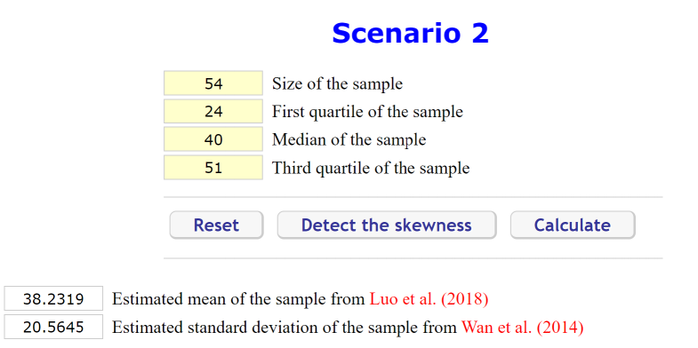
Figure 3: An example for implementing the online calculator under scenario $S_{2}$, with the sample data from the nonsurvivors group in Zhou et al.[23]

Last but not least, we have also launched an online calculator for practitioners to implement the flow chart including the skewness test and the data transformation at http://www.math.hkbu.edu.hk/~tongt/papers/median2mean.html. Our online calculator is very user-friendly, and for illustration, we consider scenario $\mathcal{S}_{2}$ with the reported data $\{q_{1},m,q_{3};n\}=\{24,40,51;54\}$ from the nonsurvivors group in Zhou et al.[23] As shown in Figure 3, with the summary data in the corresponding entries, one can click on the Detect the skewness button to examine whether the data are skewed away from normality. A popup window will then appear showing the test result, and specifically for the given data, there is no significant evidence to show that the data are skewed. In view of this, we further click on the Calculate button to perform data transformation by the normal-based methods, which yields the sample mean estimate as 38.2319 by Luo et al.[3] and the sample SD estimate as 20.5645 by Wan et al.[2]

4 Simulation studies

In this section, we conduct simulation studies to evaluate the performance of the three skewness tests. We first assess the type I error rates of the new tests with the asymptotic, exact, and approximated critical values at the significance level of 0.05, and then compute and compare their statistical power under four skewed alternative distributions. Moreover, we also conduct a simulated meta-analysis to demonstrate the usefulness of the skewness tests in practice.

4.1 Type I error rates

To examine whether the type I error rates are well controlled, we first generate a sample of size $n$ from the null distribution, and without loss of generality, we consider the standard normal distribution. Then for the proposed test under scenario $\mathcal{S}_{1}$, we record the summary statistics $\{a,m,b\}$ from the simulated sample, and compute the observed value of the test statistic $t_{1,{\rm obs}}$ by (2). Further by comparing $t_{1,{\rm obs}}$ with the asymptotic, exact, and approximated critical values respectively, we can make a decision whether to reject the null hypothesis, or equivalently, whether a type I error will be made. Finally, we repeat the above procedure for 1,000,000 times with $n$ ranging from 5 to 401, compute the type I error rates for the three different tests as reported in Figure 4.

It is evident from the simulated results that, under scenario $\mathcal{S}_{1}$, the proposed tests with the exact and approximated critical values perform nearly the same, and they both control the type I error rates at the significance level of 0.05 regardless of the sample size.

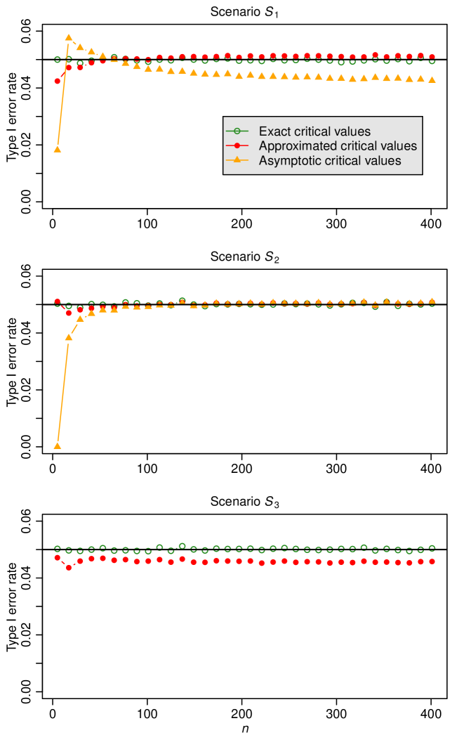
Figure 4: The type I error rates for the proposed test statistics under the three scenarios for $n$ up to 401. The solid orange triangles represent the tests with the asymptotic critical values, the empty green points represent the tests with the exact critical values, and the solid red points represent the tests with the approximated critical values.

This, from another perspective, demonstrates that our approximate formula of the critical values is rather accurate and can be recommended for practical use. In contrast, for the asymptotic test with the null distribution specified in (3), the type I error rates are less well controlled, either inflated or too conservative. For example, the type I error rate is as high as 0.057 when $n=17$, and it is always less than 0.05 when $n$ is large, even though the simulated type I error rate does converge to the significance level as $n$ goes to infinity which coincides with the theoretical result of Theorem 1 in Appendix A.

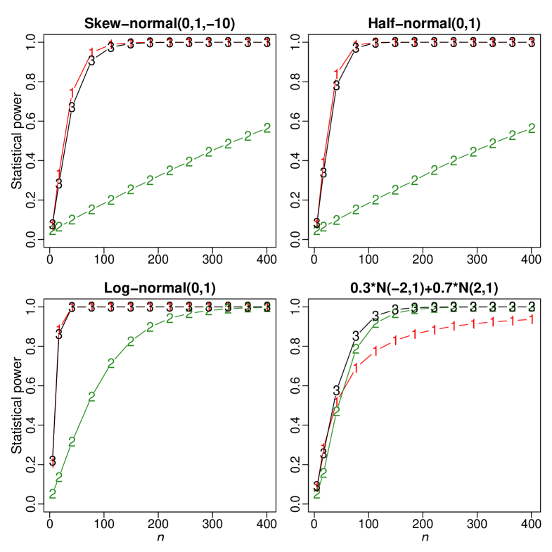
Figure 5: The statistical power of the proposed tests under the three scenarios for $n$ up to 401. “1” represents the statistical power under scenario $\mathcal{S}_{1}$, “2” represents the statistical power under scenario $\mathcal{S}_{2}$, and “3” represents the statistical power under scenario $\mathcal{S}_{3}$.

To assess the type I error rates under the last two scenarios, we record instead the summary statistics $\{q_{1},m,q_{3}\}$ or $\{a,q_{1},m,q_{3},b\}$ from the simulated sample, compute the observed value of the test statistic by (5) or (7), and then compare it with the different critical values to determine whether the null hypothesis will be rejected. Under scenario $\mathcal{S}_{2}$, the tests with the exact and approximated critical values both perform well and control the type I error rates. While for the asymptotic test with the normal approximation in (6), it does not provide a good performance when $n$ is small. In particular when $n=5$, the type I error rate will be nearly zero so that the test will be extremely conservative. Under scenario $\mathcal{S}_{3}$, given that the asymptotic test is not available, we thus report the type I error rates for the tests with the exact and approximated critical values only. Both tests control the type I error rates and they perform equally well for any fixed sample size.

4.2 Statistical power

In this section, we assess the ability of the three tests for detecting the skewness when the alternative distribution is skewed. For this purpose, we reconsider the four normal-related distributions in Section 2, Skew-normal$(0,1,-10)$, Half-normal$(0,1)$, Log-normal$(0,1)$ and 0.3*$N(-2,1)$+0.7*$N(2,1)$, as the alternative distributions for all the tests under different scenarios. Then to numerically compute the statistical power, we follow the same procedure as in Section 4.1 except that the sample data are now generated from the alternative distributions rather than the standard normal distribution. In addition, since the asymptotic test is suboptimal and the other two tests perform nearly the same, we report the simulated power only for the tests with the approximated critical values in Figure 5 based on 1,000,000 simulations.

For the test under scenario $\mathcal{S}_{1}$, we note that it is always very powerful, in particular for the three unimodal alternative distributions. This is mainly because the extreme order statistics, including the minimum and maximum values, are very sensitive to the tail behavior of the underlying distribution. In contrast, the intermediate order statistics, including the first and third quartiles, behave more stably and are less affected by the tail distributions [27]. As a consequence, the test under scenario $\mathcal{S}_{2}$ is often less powerful in detecting the skewness of data, as those reflected in the power curves for the three unimodal alternative distributions. But there are also exceptional cases. Specifically, for the mixture-normal distribution, since the two tails are both normally shaped, the minimum and maximum values behave similarly so that the mid-range, $(a+b)/2$, is quite stable along with the sample size, and consequently, it diminishes the ability of detecting the skewness. On the other side, we note that the median is closer to the third quartile rather than to the first quartile, and so the test under scenario $\mathcal{S}_{2}$ turns out to be more powerful than the test under scenario $\mathcal{S}_{1}$ in the mixture-normal case. Finally for the test under scenario $\mathcal{S}_{3}$, since it takes into account both the extreme and intermediate order statistics, it is not surprising that it always performs better than, or at least as well as, the other two tests in most settings.

To sum up, by virtue of the well-controlled type I error rates and the reasonable statistical power, we believe that our easy-to-implement tests with the approximated critical values will have potential to be widely adopted for detecting the skewness away from normality based on the five-number summary with application to meta-analysis.

4.3 Simulated meta-analysis

To further demonstrate the usefulness of the proposed skewness tests, we also conduct a simulated meta-analysis consisting of 10 studies with normal data and 5 studies with non-normal data. Following the random-effects model [28], we first generate the individual means $\mu_{i}$, $i=1,2,\ldots,15$, from the between-study distribution $N(\mu,\tau^{2})$. Then for each study, we generate a sample of size $n_{i}$ from $N(\mu_{i},\sigma_{i}^{2})$ for $i=1,\dots,10$, and from Skew-normal$(\delta_{i},\omega_{i},\alpha_{i})$ for $i=11,\dots,15$, where $\delta_{i}=\mu_{i}-\omega_{i}\sqrt{2\alpha_{i}^{2}/[\pi(1+\alpha_{i}^{2})]}$ ensuring that the mean of the skew-normal distribution is also $\mu_{i}$. Moreover, for the first 10 studies, we follow a similar setting as in Brockwell and Gordon[29] and consider $\mu=0.5$, $\tau^{2}=0.04$, $\sigma_{i}^{2}=1$ for $i=1,\dots,10$, and $n_{i}=n$ for all the studies. While for the last 5 studies, we let $\omega_{i}=5$ for $i=11,\dots,15$, and $\alpha_{11}=-0.1$ and $\alpha_{i}=-10$ for $i=12,\dots,15$ to represent the different levels of skewness. Lastly, it is noteworthy that we have also considered more general settings including unequal within-study variances and unequal sample sizes, and the comparison results remain similar.

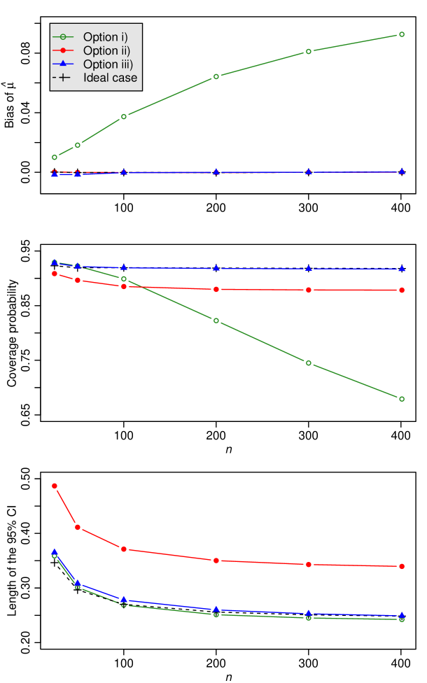
Figure 6: The bias of $\hat{\mu}$, the coverage probability and the average length for the 95% CI for $\mu$ under scenario $\mathcal{S}_{1}$ with $n$ up to 401, where option i) represents that all the 15 studies are included, option ii) represents that only the first 5 studies reporting the sample mean and SD are included, option iii) represents that the first 5 studies plus all other studies passing the skewness test are included, and the ideal case represents that the 10 normal studies are included with their true sample means and SDs.

After the dataset is generated, we report the sample mean and SD as the summary statistics for the first 5 studies, but instead report the minimum, median, and maximum values, i.e., under scenario $\mathcal{S}_{1}$, for the other 10 studies. We further consider three options to carry out the meta-analysis using i) all the 15 studies, ii) only the first 5 studies reporting the sample mean and SD, and iii) the first 5 studies plus all other studies passing the skewness test. Moreover, as an ideal case for comparison, we also conduct the meta-analysis based on the true sample means and SDs of the generated data from the 10 normal studies. Finally, by considering the mean value as the effect size, we apply the DerSimonian and Laird method [30] for meta-analysis and report the bias of the effect size estimate $\hat{\mu}$, the coverage probability and the average length of the 95% confidence interval (CI) for $\mu$, in Figure 6 for the sample size up to 401 based on a total of 500,000 simulations.

From the top panel of Figure 6, it is evident that the effect size estimate $\hat{\mu}$ under option i) with all 15 studies being included tends to be significantly biased. In contrast, options ii) and iii) are both able to control the estimation bias of $\hat{\mu}$, nearly as well as the ideal case for benchmarking. From the middle and bottom panels of Figure 6, we also observe that option ii) not only suffers from a lower coverage probability, but also has a wider CI compared to option iii) and the ideal case. This is mainly because option ii) loses valuable information by excluding the normal studies reported with the five-number summary, and consequently yields less efficient estimation of the effect size. Taken together, our new option iii) with the flow chart in Figure 1 can effectively detect and exclude some very skewed studies away from the subsequent meta-analysis, and as seen from the simulation results, it performs equally well as the ideal case except that the average length of the CI is slightly longer.

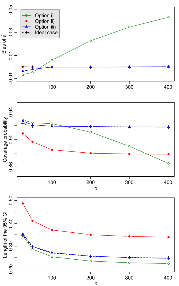
Figure 10: The bias of $\hat{\mu}$, the coverage probability and the average length of the 95% CI for $\mu$ under scenario $\mathcal{S}_{3}$ with $n$ up to 401, where option i) represents that all the 15 studies are included, option ii) represents that only the first 5 studies reporting the sample mean and SD are included, option iii) represents that the first 5 studies plus all other studies passing the skewness test are included, and the ideal case represents that the 10 normal studies are included with their true sample means and SDs.

Finally, to save space, we present the simulation results under scenarios $\mathcal{S}_{2}$ and $\mathcal{S}_{3}$ in Appendix B; for more details, see Figures 9 and 10. It is evident that the comparison results under scenario $\mathcal{S}_{3}$ are similar to those under scenario $\mathcal{S}_{1}$. While for scenario $\mathcal{S}_{2}$, by noting that the test statistic $T_{2}$ is less powerful in detecting the skewness of data as clarified in Section 4.2 through Figure 5, option iii) may not be able to exclude some very skewed studies from the meta-analysis. As a consequence, it may also yield a biased effect size estimate, even though it is apparently better than option i). On the other hand, thanks to the flow chart in Figure 1 that allows more studies to be included in the meta-analysis, option iii) is able to provide a narrower or much narrower CI compared to option ii). To summarize, although option iii) does not perform equally well as the ideal case under scenario $\mathcal{S}_{2}$, it is still comparable to, or better than, the other two options based on our simulation results.

5 Real data analysis

To illustrate the usefulness of the skewness tests as well as the flow chart, we now revisit the motivating example in Section 2, where Wu and Yang[19] investigated the impact of COVID-19 on the liver dysfunction. Specifically, we first present their meta-analytical results and then apply our new flow chart to reanalyze the example, followed by a comparison made between their results and our new results.

5.1 Original results in Wu and Yang[19]

To deal with the studies reported with the first quartile, the median and the third quartile together with the sample size, Wu and Yang[19] applied the data transformation in Hozo et al.[1] to obtain the sample mean and SD estimates, and then performed the meta-analysis with the forest plot in panel (a) of Figure 7. The random-effects model was used to pool the studies, which yielded the overall standardized mean difference (SMD) 1.34 with the 95% CI being $[-0.47,3.16]$. Given that the 95% CI of the overall effect size covers zero, Wu and Yang[19] concluded that the impact of COVID-19 on the ALT level is not statistically significant. However, noting that an extremely large heterogeneity with $p<0.01$ and $I^{2}=99\%$ is observed, the random-effects model may not be sufficient to well synthesize the included studies, and thus the final conclusion can be problematic.

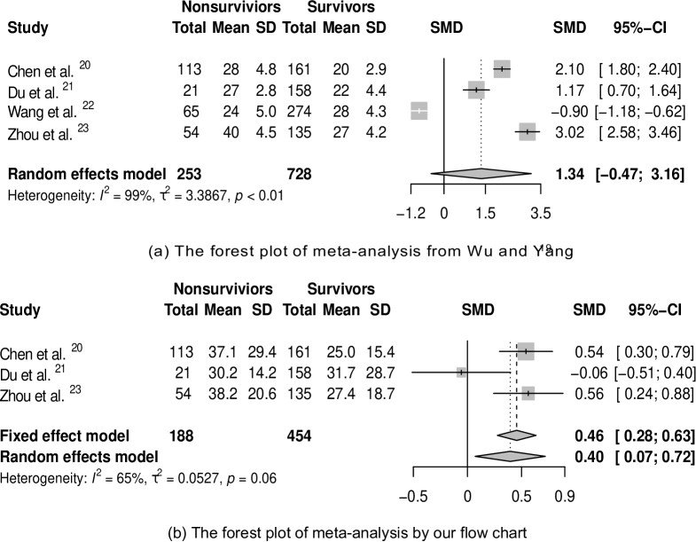
Figure 7: The forest plots of the meta-analyses from Wu and Yang[19] and by our new flow chart are presented in panels (a) and (b), respectively.

5.2 New results by our flow chart

To reanalyze the impact of COVID-19 on the liver dysfunction, we follow the flow chart in Figure 1 as a practical guideline for meta-analysis, where the first and foremost step is to identify whether some studies are significantly skewed. Since the summary statistics for the four studies are all reported under scenario $\mathcal{S}_{2}$, we thus apply the test statistic $T_{2}$ to conduct the skewness test. Specifically, by Section 3.2, we compute the absolute value of the observed $T_{2}$ for each data, compare it with the approximated critical value at the significance level of 0.05, and then report the test result in panel (a) of Table 3. It is surprising to see that only the last study passes the skewness test for both nonsurvivors and survivors groups, and consequently, Luo et al.[3] and Wan et al.[2] can be applied to this study for obtaining the sample mean and SD estimates.

Moreover, recall that the skewed data all display a positively skewed pattern as observed, and in the medical literature, the log transformation is frequently used to normalize such data [31, 32, 33]. Following this, we also apply a log transformation to the data from the three skewed studies, and then redo the skewness test using the log scale data. From the test results in panel (b) of Table 3, it is unfortunate that the nonsurvivors group in Wang et al.[22], once again, fails to pass the skewness test, indicating an unacceptably large degree of skewness on the original data.

Table 3: The absolute values of the observed $T_{2}$, the critical values at the significance level of 0.05, and the test results for the original and log scale data from the corresponding studies are reported in panels (a) and (b), respectively.

(a) Test results for the original data
Study	Nonsurvivors			Survivors
	$|T_{2}|$	Critical value	Decision	$|T_{2}|$	Critical value	Decision
Chen et al.[20]	0.310	0.249	Reject	0.395	0.209	Reject
Du et al.[21]	0.176	0.565	Not reject	0.396	0.211	Reject
Wang et al.[22]	0.667	0.327	Reject	0.154	0.160	Not reject
Zhou et al.[23]	0.185	0.359	Not reject	0.04	0.228	Not reject

(b) Test results for the log scale data
Study	Nonsurvivors			Survivors
	$|T_{2}|$	Critical value	Decision	$|T_{2}|$	Critical value	Decision
Chen et al.[20]	0.083	0.249	Not reject	0.205	0.209	Not reject
Du et al.[21]	0.016	0.565	Not reject	0.151	0.211	Not reject
Wang et al.[22]	0.495	0.327	Reject	0.075	0.160	Not reject

For the skewed studies, as per the proposed flow chart in Figure 1, one may exclude the skewed studies from meta-analysis for normal data, or apply the non-normal data transformation methods for skewed studies, or perform the subgroup analysis that separates the normal and skewed studies. For this case, note that there are only four studies included and further separating them into subgroups will make certain subgroup(s) include only one or two studies, which may not yield reliable results. Therefore, we propose to take advantages of the first two options. Specifically, we exclude Wang et al.[22] from the subsequent meta-analysis given that its nonsurvivors group is extremely skewed and to the best of our knowledge, there is little work on directly meta-analyzing the skewed data with unknown distributions. For both studies that pass the skewness test under the log scale (Chen et al.[20] and Du et al.[21]), we treat their original data as log-normally distributed and estimate the sample means and SDs by Shi et al.[33]

Then by following the setting in Wu and Yang[19], we conduct the meta-analysis with the SMD as the effect size and the forest plot is presented in panel (b) of Figure 7. Noting that a moderate heterogeneity is observed with $I^{2}=65\%$ and $p=0.06$, we refer to the random-effects model for the decision making [28]. Specifically, the random-effects model yields the SMD 0.40 with the 95% CI being $[0.07,0.72]$, which indicates that the nonsurvivors group has a significantly higher ALT level than the survivors group. Meanwhile, it is also worth mentioning that if we exclude all skewed studies but only include Zhou et al.[23] in the meta-analysis according to our first option, with the SMD being 0.56 and its 95% CI being $[0.24,0.88]$, the conclusion remains the same as above. Consequently, we conclude that the nonsurvivors group has a significantly higher ALT level than the survivors group.

Of interest, the conclusion is converted when we compare our new results with those in Wu and Yang.[19] With the conflicting conclusions, it calls for more studies to confirm the final conclusion so as to give a proper guideline in practice. Meanwhile, more attention and methodologies are warranted to deal with the skewed studies in meta-analysis.

6 Conclusion

For clinical studies with continuous outcomes, the sample mean and standard deviation (SD) are routinely reported as the summary statistics when the data are normally distributed. While in some studies, however, researchers may report the whole or part of the five-number summary, mainly because the data from the specific studies are potentially skewed away from normality. For the studies with skewed data, if we include them in the classical meta-analysis for normal data, it may yield unreliable or even misleading conclusions. In this paper, we develop three new tests for detecting the skewness of data for the flow chart of the meta-analysis based on the sample size and the five-number summary. If the skewness test is not rejected, we then apply the normal-based transformation methods to recover the sample mean and SD from the five-number summary. Otherwise, we provide practitioners with three options for different cases. Simulation studies are carried out to demonstrate that the skewness tests yield satisfying statistical power with the type I error controlled. The usefulness of the flow chart including the skewness tests has also been demonstrated by the simulated meta-analysis as well as a real data example. An online calculator is provided for performing the skewness test and the data transformation in the flow chart. We also summarize the three skewness tests together with the critical regions of size 0.05 in Table 4.

Table 4: The summary table of the skewness tests under the three scenarios.

Scenario	Test statistic	Critical region of size 0.05
$\mathcal{S}_{1}$	$T_{1}=\dfrac{a+b-2m}{b-a}$	$|T_{1}|>\dfrac{1}{\ln(n+9)}+\dfrac{2.5}{n+1}$
$\mathcal{S}_{2}$	$T_{2}=\dfrac{q_{1}+q_{3}-2m}{q_{3}-q_{1}}$	$|T_{2}|>\dfrac{2.65}{\sqrt{n}}-\dfrac{6}{n^{2}}$
$\mathcal{S}_{3}$	$T_{3}=\max\left\{\dfrac{2.65\ln(0.6n)}{\sqrt{n}}|T_{1}|,|T_{2}|\right\}$	$T_{3}>\dfrac{3}{\sqrt{n}}-\dfrac{40}{n^{3}}$

To further clarify, if a study passes the skewness test, it does not necessarily mean that the data are normally distributed, but rather there is no significant evidence to claim that the data are significantly skewed. And without further evidence (for or against) whether the studies passing the skewness test are truly normally distributed, our flow chart in Figure 1 suggests to still include them into the subsequent meta-analysis. As otherwise, we will face another dilemma that valuable information may be excluded from meta-analysis so that the final conclusion is less reliable or even misleading, especially when a large proportion of studies are reported with the five-number summary. Future research, either theoretically or numerically, are warranted to further assess the studies passing the skewness test. Lastly, thanks to the good performance of the skewness tests as well as the flow chart, together with the online calculator at http://www.math.hkbu.edu.hk/~tongt/papers/median2mean.html, we expect they may have potential to be widely adopted in meta-analysis and evidence-based practice.

Appendix A: Theoretical results

Lemma 1.

Let $Z_{1},Z_{2},\ldots,Z_{n}$ be a random sample from the standard normal distribution, and $Z_{(1)}\leq Z_{(2)}\leq\cdots\leq Z_{(n)}$ be the corresponding order statistics. We have

$$(Z_{(1)},Z_{(2)},\ldots,Z_{(n)})\overset{d}{=}(-Z_{(n)},-Z_{(n-1)},\ldots,-Z_{(1)}),$$

where $\overset{d}{=}$ represents that two random vectors follow the same distribution. Thus it is evident that

$$E(Z_{(i)})=-E(Z_{(n-i+1)}),\quad 1\leq i\leq n.$$

Specifically, by letting $n=4Q+1$ with $Q$ being a positive integer, it directly follows that $E(Z_{(2Q+1)})=0$, $E(Z_{(Q+1)})=-E(Z_{(3Q+1)})$ and $E(Z_{(1)})=-E(Z_{(n)})$. For a random sample $X_{1},X_{2},\ldots,X_{n}$ from the normal distribution with mean $\mu$ and variance $\sigma^{2}$, where $X_{(1)}\leq X_{(2)}\leq\cdots\leq X_{(n)}$ represents its order statistics, we have

$$E(X_{(i)})=\mu+\sigma E(Z_{(i)}),\quad 1\leq i\leq n.$$

Theorem 1.

Under scenario $\mathcal{S}_{1}=\{a,m,b;n\}$, as $n\rightarrow\infty$ under the null hypothesis of normality, we have

$$\sqrt{2\ln(n)}\xi(n)\left(\dfrac{a+b-2m}{b-a}\right)\overset{D}{\longrightarrow}{\rm Logistic}(0,1),$$

where $\xi(n)=2\Phi^{-1}[(n-0.375)/(n+0.25)]$.

Proof. Under the null hypothesis of normality, it is evident that

$$\dfrac{a+b-2m}{2\sigma}=\dfrac{Z_{(1)}+Z_{(n)}}{2}-Z_{(2Q+1)}.$$

According to Ferguson[25], as $n\rightarrow\infty$, we have

$$\sqrt{2\ln(n)}\left(\dfrac{Z_{(1)}+Z_{(n)}}{2}\right)\overset{D}{\longrightarrow}{\rm Logistic}(0,0.5)$$

and

$$\sqrt{n}Z_{(2Q+1)}\overset{D}{\longrightarrow}N\left(0,\dfrac{\pi}{2}\right),$$

where $\overset{D}{\longrightarrow}$ denotes the convergence in distribution. Thus under the null hypothesis, it is evident that

$$\sqrt{2\ln(n)}\left(\dfrac{a+b-2m}{2\sigma}\right)=I_{1}-I_{2},$$

where

$$I_{1} =\sqrt{2\ln(n)}\left(\dfrac{Z_{(1)}+Z_{(n)}}{2}\right),$$

$$I_{2} =\sqrt{2\ln(n)}Z_{(2Q+1)}.$$

As $n\rightarrow\infty$, $I_{1}\overset{D}{\longrightarrow}{\rm Logistic}(0,0.5)$ and $I_{2}\overset{P}{\longrightarrow}0$, where $\overset{P}{\longrightarrow}$ denotes the convergence in probability. Then by Slutsky’s Theorem, as $n\rightarrow\infty$, we conclude that

$$\sqrt{2\ln(n)}\left(\dfrac{a+b-2m}{\sigma}\right)\overset{D}{\longrightarrow}{\rm Logistic}(0,1).$$

According to Wan et al.[2], it is evident that $\hat{\sigma}_{1}=(b-a)/\xi(n)$ is a consistent estimator of the standard deviation $\sigma$ for a normal distribution. With $\sigma$ estimated by $\hat{\sigma}_{1}$ and noting that $\xi(n)$ is the fixed value for any given $n$, the final test statistic is derived as

$$T_{1}=\dfrac{a+b-2m}{b-a}$$

and again by Slutsky’s Theorem as $n\rightarrow\infty$, $\sqrt{2\ln(n)}\xi(n)T_{1}\overset{D}{\longrightarrow}{\rm Logistic}(0,1)$.

Theorem 2.

Under scenario $\mathcal{S}_{1}=\{a,m,b;n\}$, the null distribution of the test statistic $T_{1}=(a+b-2m)/(b-a)$ is

$$f_{1}(t_{1})= \iint\limits_{\mathcal{D}}\dfrac{n!}{[(2Q-1)!]^{2}}\cdot\dfrac{v-u}{2}\cdot\phi(u)\phi(v)\phi\left(\dfrac{u+v}{2}-\dfrac{t_{1}(v-u)}{2}\right)$$

$$\cdot\left[\Phi\left(\dfrac{u+v}{2}-\dfrac{t_{1}(v-u)}{2}\right)-\Phi(u)\right]^{2Q-1}$$

$$\cdot\left[\Phi(v)-\Phi\left(\dfrac{u+v}{2}-\dfrac{t_{1}(v-u)}{2}\right)\right]^{2Q-1}{\rm d}u{\rm d}v,$$ (8)

where $\mathcal{D}$ is the integral area that satisfies $u\leq v$. Furthermore, the null distribution of $T_{1}$ is symmetric about zero.

Proof. Denote $z_{1}=Z_{(1)}$, $z_{m}=Z_{(2Q+1)}$ and $z_{n}=Z_{(n)}$. Recall that for $(z_{1},z_{m},z_{n})$, we have the joint distribution as

$$g_{1}(z_{1},z_{m},z_{n})=\dfrac{n!}{[(2Q-1)!]^{2}}\phi(z_{1})\phi(z_{m})\phi(z_{n})[\Phi(z_{m})-\Phi(z_{1})]^{2Q-1}[\Phi(z_{n})-\Phi(z_{m})]^{2Q-1}.$$

It is evident that $(z_{1},z_{m},z_{n})\rightarrow(u,t_{1},v)$ is a one-to-one mapping, where $u=z_{1}$, $t_{1}=(z_{1}+z_{n}-2z_{m})/(z_{n}-z_{1})$ and $v=z_{n}$, or equivalently, $z_{1}=u$, $z_{m}=(u+v)/2-t_{1}(v-u)/2$ and $z_{n}=v$. Thus we have the determinant of the Jacobian matrix as

$$\left|\begin{array}[]{cccc}1&0&0\\ \dfrac{1+t_{1}}{2}&\dfrac{u-v}{2}&\dfrac{1-t_{1}}{2}\\ 0&0&1\\ \end{array}\right|=\dfrac{v-u}{2}.$$

With the Jacobian transformation, we derive the joint distribution of $(u,t_{1},v)$ as

$$g_{1}^{*}(u,t_{1},v)= \dfrac{n!}{[(2Q-1)!]^{2}}\cdot\dfrac{v-u}{2}\cdot\phi(u)\phi(v)\phi\left(\dfrac{u+v}{2}-\dfrac{t_{1}(v-u)}{2}\right)$$

$$\cdot\left[\Phi\left(\dfrac{u+v}{2}-\dfrac{t_{1}(v-u)}{2}\right)-\Phi(u)\right]^{2Q-1}$$

$$\cdot\left[\Phi(v)-\Phi\left(\dfrac{u+v}{2}-\dfrac{t_{1}(v-u)}{2}\right)\right]^{2Q-1}.$$

Further by taking the integrals with respect to $u$ and $v$, we achieve the sampling distribution of $T_{1}$ in (Appendix A: Theoretical results) under the null hypothesis.

In addition, by Lemma 1, we have

$$(Z_{(1)},Z_{(2Q+1)},Z_{(n)})\overset{d}{=}(-Z_{(n)},-Z_{(2Q+1)},-Z_{(1)}).$$

Thus under the null hypothesis, it is evident that

$$T_{1}=\dfrac{Z_{(1)}+Z_{(n)}-2Z_{(2Q+1)}}{Z_{(n)}-Z_{(1)}}\quad{\rm and}\quad-T_{1}=\dfrac{(-Z_{(n)})+(-Z_{(1)})-2(-Z_{(2Q+1)})}{(-Z_{(1)})-(-Z_{(n)})},$$

and therefore the null distribution of $T_{1}$ is symmetric about zero.

Theorem 3.

Under scenario $\mathcal{S}_{2}=\{q_{1},m,q_{3};n\}$, as $n\rightarrow\infty$ under the null hypothesis of normality, we have

$$0.74\sqrt{n}\left(\dfrac{q_{1}+q_{3}-2m}{q_{3}-q_{1}}\right)\overset{D}{\longrightarrow}N(0,1).$$

Proof. Under the null hypothesis of normality, it is evident that

$$\dfrac{q_{1}+q_{3}-2m}{\sigma}=Z_{(Q+1)}+Z_{(3Q+1)}-2Z_{(2Q+1)}.$$

According to Ferguson[25], as $n\rightarrow\infty$, we have that $(Z_{(Q+1)},Z_{(2Q+1)},Z_{(3Q+1)})$ follows asymptotically a tri-variate normal distribution with mean vector $(\Phi^{-1}(0.25),0,\Phi^{-1}(0.75))$ and covariance matrix $\Sigma$, where

$$\Sigma=\dfrac{1}{n}\left(\begin{matrix}1.86&0.99&0.62\\ 0.99&\pi/2&0.99\\ 0.62&0.99&1.86\end{matrix}\right).$$

Then by the Delta method, as $n\rightarrow\infty$, we have

$$Z_{(Q+1)}+Z_{(3Q+1)}-2Z_{(2Q+1)}=(1,-2,1)\left(\begin{array}[]{c}Z_{(Q+1)}\\ Z_{(2Q+1)}\\ Z_{(3Q+1)}\end{array}\right)\overset{D}{\longrightarrow}N(0,3.32/n).$$

Therefore, we achieve the asymptotic normality under the null hypothesis that

$$0.55\sqrt{n}\left(\dfrac{q_{1}+q_{3}-2m}{\sigma}\right)\overset{D}{\longrightarrow}N(0,1).$$

According to Wan et al.[2], it is evident that $\hat{\sigma}_{2}=(q_{3}-q_{1})/\eta(n)$ is a consistent estimator of the standard deviation $\sigma$ for a normal distribution, where $\eta(n)=2\Phi^{-1}[(0.75n-0.125)/(n+0.25)]$. Further by Theorem 1 in Shi et al.[4], as $n\rightarrow\infty$, $\eta(n)=2\Phi^{-1}(0.75)=1.35$. With $\sigma$ estimated by $\hat{\sigma}_{2}$ and noting $\eta(n)$ is a constant, we propose the test statistic as

$$T_{2}=\dfrac{q_{1}+q_{3}-2m}{q_{3}-q_{1}}$$

and by Slutsky’s Theorem as $n\rightarrow\infty$, $0.74\sqrt{n}T_{2}\overset{D}{\longrightarrow}\text{N}(0,1)$.

Theorem 4.

Under scenario $\mathcal{S}_{2}=\{q_{1},m,q_{3};n\}$, the null distribution of the test statistic $T_{2}=(q_{1}+q_{3}-2m)/(q_{3}-q_{1})$ is

$$f_{2}(t_{2})= \iint\limits_{\mathcal{D}}\dfrac{n!}{[Q!(Q-1)!]^{2}}\phi(x)\phi\left(\dfrac{x+y}{2}-\dfrac{t_{2}(y-x)}{2}\right)\phi(y)[\Phi(x)]^{Q}[1-\Phi(y)]^{Q}$$

$$\cdot\left[\Phi\left(\dfrac{x+y}{2}-\dfrac{t_{2}(y-x)}{2}\right)-\Phi(x)\right]^{Q-1}$$

$$\cdot\left[\Phi(y)-\Phi\left(\dfrac{x+y}{2}-\dfrac{t_{2}(y-x)}{2}\right)\right]^{Q-1}{\rm d}x{\rm d}y,$$ (9)

where $\mathcal{D}$ is the integral area that satisfies $x\leq y$. Furthermore, the null distribution of $T_{2}$ is symmetric about zero.

Proof. Denote $z_{q_{1}}=Z_{(Q+1)}$, $z_{m}=Z_{(2Q+1)}$ and $z_{q_{3}}=Z_{(3Q+1)}$. Recall that for $(z_{q_{1}},z_{m},z_{q_{3}})$, we have the joint distribution as

$$g_{2}(z_{q_{1}},z_{m},z_{q_{3}})= \dfrac{n!}{Q!(Q-1)!(Q-1)!Q!}\phi(z_{q_{1}})\phi(z_{m})\phi(z_{q_{3}})[\Phi(z_{q_{1}})]^{Q}[\Phi(z_{m})-\Phi(z_{q_{1}})]^{Q-1}$$

$$[\Phi(z_{q_{3}})-\Phi(z_{m})]^{Q-1}[1-\Phi(z_{q_{3}})]^{Q}.$$

It is evident that $(z_{q_{1}},z_{m},z_{q_{3}})\rightarrow(x,t_{2},y)$ is a one-to-one mapping, where $x=z_{q_{1}}$, $t_{2}=(z_{q_{1}}+z_{q_{3}}-2z_{m})/(z_{q_{3}}-z_{q_{1}})$ and $y=z_{q_{3}}$, or equivalently, $z_{q_{1}}=x$, $z_{m}=(x+y)/2-t_{2}(y-x)/2$ and $z_{q_{3}}=y$. Thus we have the determinant of the Jacobian matrix as

$$\left|\begin{array}[]{cccc}1&0&0\\ \dfrac{1+t_{2}}{2}&\dfrac{x-y}{2}&\dfrac{1-t_{2}}{2}\\ 0&0&1\\ \end{array}\right|=\dfrac{y-x}{2}.$$

With the Jacobian transformation, we derive the joint distribution of $(x,t_{2},y)$ as

$$g_{2}^{*}(x,t_{2},y)= \dfrac{n!}{[Q!(Q-1)!]^{2}}\phi(x)\phi\left(\dfrac{x+y}{2}-\dfrac{t_{2}(y-x)}{2}\right)\phi(y)[\Phi(x)]^{Q}[1-\Phi(y)]^{Q}$$

$$\cdot\left[\Phi\left(\dfrac{x+y}{2}-\dfrac{t_{2}(y-x)}{2}\right)-\Phi(x)\right]^{Q-1}$$

$$\cdot\left[\Phi(y)-\Phi\left(\dfrac{x+y}{2}-\dfrac{t_{2}(y-x)}{2}\right)\right]^{Q-1}.$$

Further by taking the integrals with respect to $x$ and $y$, we achieve the sampling distribution of $T_{2}$ in (4) under the null hypothesis. Similar to the proof in Theorem 2, we can prove that the null distribution of $T_{2}$ is symmetric about zero.

Theorem 5.

Under scenario $\mathcal{S}_{3}=\{a,q_{1},m,q_{3},b;n\}$, the test statistic is derived as

$$T_{3}=\max\left\{\dfrac{2.65\ln(0.6n)}{\sqrt{n}}\left|\dfrac{a+b-2m}{b-a}\right|,\ \left|\dfrac{q_{1}+q_{3}-2m}{q_{3}-q_{1}}\right|\right\}.$$

Proof. Under scenario $\mathcal{S}_{3}$, by taking advantages of both extreme and intermediate order statistics, we consider to detect the skewness of data with

$$W_{3}=\max\left\{\left|\dfrac{a+b-2m}{{\rm SE}(a+b-2m)}\right|,\ \left|\dfrac{q_{1}+q_{3}-2m}{{\rm SE}(q_{1}+q_{3}-2m)}\right|\right\}.$$

Recall that in Section 3.1 of the main text, we have derived ${\rm SE}(a+b-2m)=\sigma\delta_{1}(n)$, where $\delta_{1}(n)={\rm SE}(Z_{(1)}+Z_{(n)}-2Z_{(2Q+1)})$ and $\sigma$ is estimated with $(b-a)/\xi(n)$. Similarly, we have ${\rm SE}(q_{1}+q_{3}-2m)=\sigma\delta_{2}(n)$, where $\delta_{2}(n)={\rm SE}(Z_{(Q+1)}+Z_{(3Q+1)}-2Z_{(2Q+1)})$, and $\sigma$ is estimated with $(q_{3}-q_{1})/\eta(n)$. Then, the test statistic is specified as

$$\max\left\{\dfrac{\xi(n)}{\delta_{1}(n)}|T_{1}|,\ \dfrac{\eta(n)}{\delta_{2}(n)}|T_{2}|\right\},$$

where $T_{1}=(a+b-2m)/(b-a)$ and $T_{2}=(q_{1}+q_{3}-2m)/(q_{3}-q_{1})$ are the test statistics under scenarios $\mathcal{S}_{1}$ and $\mathcal{S}_{2}$.

To simplify the presentation, we combine $\eta(n)/\delta_{2}(n)$ with $\xi(n)/\delta_{1}(n)$ in the first term so that only one coefficient $k(n)=[\xi(n)/\delta_{1}(n)]/[\eta(n)/\delta_{2}(n)]$ is needed, and meanwhile $k(n)|T_{1}|$ and $|T_{2}|$ are still comparable in scale. Further noting that $k(n)$ is difficult to compute since $\delta_{1}(n)$ and $\delta_{2}(n)$ involved do not have the explicit forms, the test statistic may not be readily accessible to practitioners. By following the asymptotic form of $k(n)$, we have provided the approximate formula as $k(n)\approx 2.65\ln(0.6n)/\sqrt{n}$ for practical use. Finally, test statistic is yielded as

$$T_{3}=\max\left\{\dfrac{2.65\ln(0.6n)}{\sqrt{n}}\left|\dfrac{a+b-2m}{b-a}\right|,\ \left|\dfrac{q_{1}+q_{3}-2m}{q_{3}-q_{1}}\right|\right\}.$$

Appendix B: Supplementary tables and figures

This appendix presents some supplementary tables and figures. Specifically, Tables 5-7 report the numerical critical values of the test statistics in Section 3 under the three scenarios at the significance level of 0.05, Figure 8 presents the approximate functions of the critical values under the three scenarios, and Figures 9 and 10 present the simulated meta-analysis results under scenarios $\mathcal{S}_{2}$ and $\mathcal{S}_{3}$, respectively.

For non-integer $Q$, the numerical critical values can be computed using the interpolation method through the following formula: $(1+[Q]-Q)c_{i,0.025}(4[Q]+1)+(Q-[Q])c_{i,0.025}(4[Q+1]+1)$ for $i=1,2,3$ respectively, where $[Q]$ represents the integer part of $Q$. As an example, we now consider scenario $\mathcal{S}_{1}$ with $n=6$ and thus $Q=1.25$. By Table 5, the critical values for the two adjacent integers $Q=1$ and $Q=2$ are 0.7792 and 0.5706, respectively. Further by the interpolation formula, the critical value for $Q=1.25$ can be computed as 0.72705 ($=0.75*0.7792+0.25*0.5706$). In addition, we can also apply the approximate formula $1/\ln(n+9)+2.5/(n+1)$ in Section 3.1 to compute the critical value for $n=6$, yielding a value of 0.72641 which is very close to the interpolated value at 0.72705.

Table 5: The numerical values of $c_{1,0.025}(n)$ for $1\leq Q\leq 100$, where $n=4Q+1$.

$Q$	$c_{1,0.025}(n)$	$Q$	$c_{1,0.025}(n)$	$Q$	$c_{1,0.025}(n)$	$Q$	$c_{1,0.025}(n)$	$Q$	$c_{1,0.025}(n)$
1	0.7792	21	0.2505	41	0.2094	61	0.1920	81	0.1805
2	0.5706	22	0.2464	42	0.2087	62	0.1905	82	0.1803
3	0.4964	23	0.2433	43	0.2072	63	0.1903	83	0.1802
4	0.4413	24	0.2402	44	0.2067	64	0.1898	84	0.1794
5	0.4032	25	0.2375	45	0.2051	65	0.1892	85	0.1792
6	0.3763	26	0.2352	46	0.2042	66	0.1886	86	0.1786
7	0.3554	27	0.2332	47	0.2031	67	0.1878	87	0.1780
8	0.3395	28	0.2315	48	0.2024	68	0.1877	88	0.1778
9	0.3253	29	0.2286	49	0.2013	69	0.1867	89	0.1777
10	0.3132	30	0.2277	50	0.2000	70	0.1864	90	0.1765
11	0.3045	31	0.2243	51	0.1990	71	0.1858	91	0.1763
12	0.2956	32	0.2238	52	0.1989	72	0.1850	92	0.1762
13	0.2884	33	0.2219	53	0.1979	73	0.1848	93	0.1758
14	0.2812	34	0.2203	54	0.1974	74	0.1840	94	0.1757
15	0.2755	35	0.2183	55	0.1964	75	0.1837	95	0.1751
16	0.2708	36	0.2172	56	0.1949	76	0.1836	96	0.1747
17	0.2660	37	0.2151	57	0.1946	77	0.1823	97	0.1741
18	0.2613	38	0.2135	58	0.1938	78	0.1819	98	0.1740
19	0.2564	39	0.2128	59	0.1928	79	0.1818	99	0.1739
20	0.2535	40	0.2111	60	0.1922	80	0.1811	100	0.1735

Table 6: The numerical values of $c_{2,0.025}(n)$ for $1\leq Q\leq 100$, where $n=4Q+1$.

$Q$	$c_{2,0.025}(n)$	$Q$	$c_{2,0.025}(n)$	$Q$	$c_{2,0.025}(n)$	$Q$	$c_{2,0.025}(n)$	$Q$	$c_{2,0.025}(n)$
1	0.9463	21	0.2861	41	0.2067	61	0.1692	81	0.1471
2	0.8000	22	0.2809	42	0.2034	62	0.1681	82	0.1461
3	0.6913	23	0.2748	43	0.2019	63	0.1667	83	0.1452
4	0.6163	24	0.2685	44	0.1993	64	0.1653	84	0.1443
5	0.5594	25	0.2633	45	0.1975	65	0.1641	85	0.1437
6	0.5177	26	0.2588	46	0.1954	66	0.1627	86	0.1428
7	0.4819	27	0.2538	47	0.1936	67	0.1614	87	0.1419
8	0.4534	28	0.2494	48	0.1914	68	0.1602	88	0.1409
9	0.4297	29	0.2447	49	0.1897	69	0.1593	89	0.1405
10	0.4084	30	0.2403	50	0.1879	70	0.1583	90	0.1395
11	0.3903	31	0.2361	51	0.1854	71	0.1570	91	0.1391
12	0.3744	32	0.2339	52	0.1831	72	0.1561	92	0.1381
13	0.3608	33	0.2298	53	0.1823	73	0.1551	93	0.1376
14	0.3486	34	0.2267	54	0.1804	74	0.1538	94	0.1364
15	0.3372	35	0.2233	55	0.1785	75	0.1527	95	0.1357
16	0.3266	36	0.2204	56	0.1776	76	0.1518	96	0.1355
17	0.3179	37	0.2176	57	0.1757	77	0.1506	97	0.1345
18	0.3085	38	0.2148	58	0.1749	78	0.1496	98	0.1339
19	0.2999	39	0.2112	59	0.1721	79	0.1486	99	0.1332
20	0.2931	40	0.2080	60	0.1718	80	0.1479	100	0.1326

Table 7: The numerical values of $c_{3,0.05}(n)$ for $1\leq Q\leq 100$, where $n=4Q+1$.

$Q$	$c_{3,0.05}(n)$	$Q$	$c_{3,0.05}(n)$	$Q$	$c_{3,0.05}(n)$	$Q$	$c_{3,0.05}(n)$	$Q$	$c_{3,0.05}(n)$
1	1.0129	21	0.3214	41	0.2305	61	0.1885	81	0.1635
2	0.9062	22	0.3139	42	0.2271	62	0.1871	82	0.1626
3	0.7929	23	0.3067	43	0.2247	63	0.1856	83	0.1617
4	0.7060	24	0.3004	44	0.2223	64	0.1840	84	0.1607
5	0.6416	25	0.2948	45	0.2193	65	0.1827	85	0.1600
6	0.5898	26	0.2885	46	0.2173	66	0.1813	86	0.1587
7	0.5490	27	0.2831	47	0.2149	67	0.1802	87	0.1579
8	0.5151	28	0.2781	48	0.2129	68	0.1786	88	0.1570
9	0.4870	29	0.2738	49	0.2104	69	0.1775	89	0.1561
10	0.4630	30	0.2687	50	0.2082	70	0.1762	90	0.1556
11	0.4419	31	0.2645	51	0.2065	71	0.1747	91	0.1546
12	0.4229	32	0.2604	52	0.2043	72	0.1734	92	0.1537
13	0.4071	33	0.2564	53	0.2024	73	0.1724	93	0.1528
14	0.3929	34	0.2523	54	0.2004	74	0.1713	94	0.1522
15	0.3797	35	0.2489	55	0.1986	75	0.1700	95	0.1512
16	0.3675	36	0.2456	56	0.1971	76	0.1689	96	0.1505
17	0.3569	37	0.2419	57	0.1953	77	0.1679	97	0.1497
18	0.3473	38	0.2393	58	0.1933	78	0.1669	98	0.1489
19	0.3380	39	0.2359	59	0.1920	79	0.1657	99	0.1479
20	0.3290	40	0.2330	60	0.1902	80	0.1646	100	0.1472

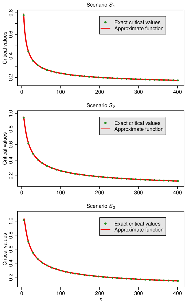
Figure 8: The green points represent the exact critical values under scenarios $\mathcal{S}_{1}$, $\mathcal{S}_{2}$ and $\mathcal{S}_{3}$, and the red lines represent the approximate functions of the critical values for $n$ up to 401.

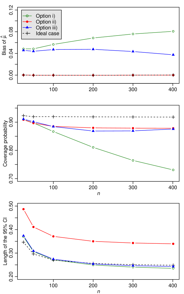
Figure 9: The bias of $\hat{\mu}$, the coverage probability and the average length of the 95% CI for $\mu$ under scenario $\mathcal{S}_{2}$ with $n$ up to 401, where option i) represents that all the 15 studies are included, option ii) represents that only the first 5 studies reporting the sample mean and SD are included, option iii) represents that the first 5 studies plus all other studies passing the skewness test are included, and the ideal case represents that the 10 normal studies are included with their true sample means and SDs.

References

- [1] Hozo SP, Djulbegovic B and Hozo I. Estimating the mean and variance from the median, range, and the size of a sample. BMC Med Res Methodol. 2005; 5: 13.
- [2] Wan X, Wang W, Liu J and Tong T. Estimating the sample mean and standard deviation from the sample size, median, range and/or interquartile range. BMC Med Res Methodol. 2014; 14: 135.
- [3] Luo D, Wan X, Liu J and Tong T. Optimally estimating the sample mean from the sample size, median, mid-range, and/or mid-quartile range. Stat Methods Med Res. 2018; 27: 1785–1805.
- [4] Shi J, Luo D, Weng H, et al. Optimally estimating the sample standard deviation from the five-number summary. Res Synth Methods. 2020; 11: 641–654.
- [5] Balduzzi S, Rücker G and Schwarzer G. How to perform a meta-analysis with R: a practical tutorial. Evid Based Ment Health. 2019; 22: 153–160.
- [6] Schwarzer G. meta: general package for meta-analysis. R package version 5.5-0; 2022. https://cran.r-project.org/web/packages/meta/meta.pdf.
- [7] Viechtbauer W. Conducting meta-analyses in R with the metafor package. J Stat Softw. 2010; 36: 1-48.
- [8] Viechtbauer W. Covert five-number summary values to means and standard deviations. metafor, R package version 3.9-16; 2022. https://wviechtb.github.io/metafor/reference/conv.fivenum.html#references-1.
- [9] Bono R, Blanca MJ, Arnau J and Gómez-Benito J. Non-normal distributions commonly used in health, education, and social sciences: a systematic review. Front Psychol. 2017; 8: 1602.
- [10] Sun RW and Cheung SF. The influence of nonnormality from primary studies on the standardized mean difference in meta-analysis. Behav Res Methods. 2020; 52: 1552-1567.
- [11] Thode HC. Testing for Normality. New York: CRC Press, 2002.
- [12] D’agostino RB, Belanger A and D’Agostino Jr RB. A suggestion for using powerful and informative tests of normality. Am Stat. 1990; 44: 316–321.
- [13] Cramér H. On the composition of elementary errors. Scand Actuar J. 1928; 1: 13–74.
- [14] Anderson TW and Darling DA. A test of goodness of fit. J Am Statist Ass. 1954; 49: 765–769.
- [15] Shapiro SS and Wilk MB. An analysis of variance test for normality (complete samples). Biometrika. 1965; 52: 591–611.
- [16] Jarque CM and Bera AK. Efficient tests for normality, homoscedasticity and serial independence of regression residuals. Econ Lett. 1980; 6: 255–259.
- [17] Altman DG and Bland JM. Statistics notes: detecting skewness from summary information. Br Med J. 1996; 313: 1200.
- [18] Forbes C, Evans M, Hastings N and Peacock B. Statistical Distributions. Hoboken: John Wiley & Sons, 2011.
- [19] Wu ZH and Yang DL. A meta-analysis of the impact of COVID-19 on liver dysfunction. Eur J Med Res. 2020; 25: 54.
- [20] Chen T, Dai Z, Mo P, et al. Clinical characteristics and outcomes of older patients with coronavirus disease 2019 (COVID-19) in Wuhan, China: a single-centered, retrospective study. J Gerontol A. 2020; 75: 1788–1795.
- [21] Du RH, Liang LR, Yang CQ, et al. Predictors of mortality for patients with COVID-19 pneumonia caused by SARS-CoV-2: a prospective cohort study. Eur Respir J. 2020; 55: 2000524.
- [22] Wang L, He W, Yu X, et al. Coronavirus disease 2019 in elderly patients: characteristics and prognostic factors based on 4-week follow-up. J Infect. 2020; 80: 639–645.
- [23] Zhou F, Yu T, Du R, et al. Clinical course and risk factors for mortality of adult inpatients with COVID-19 in Wuhan, China: a retrospective cohort study. Lancet. 2020; 395: 1054–1062.
- [24] Casella G and Berger RL. Statistical Inference. Carlifornia: Duxbury Press, 2002.
- [25] Ferguson TS. A Course in Large Sample Theory. London: Chapman and Hall, 1996.
- [26] Groeneveld RA and Meeden G. Measuring skewness and kurtosis. J R Statist Soc D. 1984; 33: 391–399.
- [27] Gather U and Tomkins J. On stability of intermediate order statistics. J Stat Plan Inference. 1995; 45: 175–183.
- [28] Higgins JP and Green S. Cochrane Handbook for Systematic Reviews of Interventions. Chichester: John Wiley and Sons, 2008.
- [29] Brockwell SE and Gordon IR. A comparison of statistical methods for meta-analysis. Stat Med. 2001; 20: 825–840.
- [30] DerSimonian R and Laird N. Meta-analysis in clinical trials. Control Clin Trials. 1986; 7: 177–188.
- [31] Higgins JP, White IR and Anzures-Cabrera J. Meta-analysis of skewed data: combining results reported on log-transformed or raw scales. Stat Med. 2008; 27: 6072–6092.
- [32] Yamaguchi Y, Maruo K, Partlett C and Riley RD. A random effects meta-analysis model with Box-Cox transformation. BMC Med Res Methodol. 2017; 17: 109.
- [33] Shi J, Tong T, Wang Y and Genton MG. Estimating the mean and variance from the five-number summary of a log-normal distribution. Stat Interface. 2020; 13: 519-531.