Granger causality of bivariate stationary curve time series

Abstract

We study causality between bivariate curve time series using the Granger causality generalized measures of correlation. With this measure, we can investigate which curve time series Granger-causes the other; in turn, it helps determine the predictability of any two curve time series. Illustrated by a climatology example, we find that the sea surface temperature Granger-causes the sea-level atmospheric pressure. Motivated by a portfolio management application in finance, we single out those stocks that lead or lag behind Dow-Jones industrial averages. Given a close relationship between S&P 500 index and crude oil price, we determine the leading and lagging variables.

Keywords: Granger causality; G-causality; functional time series.

1 Introduction

In recent years, there has been increasing interest in studying the time series of functions observed at high frequency. In these time series, the data frequency is high enough to model itself as a curve time series and gives rise to the analysis of functional time series (see, e.g., Horváth & Kokoszka, 2012; Kokoszka & Reimherr, 2017). Examples of functional time series include intraday stock price curves with each functional observation defined as a pricing function of time points within a day (e.g., see Horváth et al., 2014; Li et al., 2020), and intraday volatility curves with each functional observation defined as a volatility function of time points within a day (e.g., see Shang et al., 2019).

Most of the existing literature focuses on statistical inference, modeling, and forecasting of a univariate functional time series. We study co-movement by observing samples of bivariate stationary curve time series. A natural question is which time series causes the other? In other words, which functional variable is the leading variable and which functional variable is the lagging variable. To address this problem, we use a measure of causality in scalar-valued univariate time series analysis, known as Granger causality: Based on a suggestion by Wiener (1956), Granger (1969) proposed a Granger causality measure that relies on the additional predictive ability of the second variable. Granger causality has since been extended and applied to a range of research fields. Granger (1980) considered testing for causality, while Granger (1988) drew a connection between causation (with a lag between cause and effect) and co-integration. Hiemstra & Jones (1994) tested linear and non-linear Granger causality in the stock price-volume relation, while Diks & Panchenko (2006) introduced a nonparametric test for Granger non-causality. In neuroscience and neuroimaging, Seth et al. (2015) applied Granger causality to study neural activity using electrophysiological and fMRI data.

The Granger causality measure has been modified to generalized measures of correlation (GMC) and Granger causality generalized measures of correlation (GcGMC) by Zheng et al. (2012). Vinod (2017) applied the GMC criterion to analyze the development of economic markets in a study of 198 countries. Further, Vinod (2019) developed a package in R (R Core Team, 2020) called “generalCorr” to implement the GMC. Allen & Hooper (2018) used the GMC criterion to analyze causal relations between the VIX, S&P 500, and the realized volatility of the S&P 500 sampled at five-minute intervals. Chen et al. (2017) extended the GMC criterion to propose a model-free feature screening approach, namely sure explained variability and independence screening. In this paper, we aim to extend GcGMC from bivariate scalar-valued time series to bivariate function-valued time series.

The outline of this paper is as follows. In Section 2, we present a background for GMC and GcGMC. In Section 3, we present a nonparametric function-on-function regression model to estimate conditional mean in function-valued GcGMC. Through a series of simulation studies in Section 4, we examine the finite-sample performance of our estimate. In Section 5, we present three data analyses for our motivating data examples in climatology and finance, respectively. Conclusions are given in Section 6.

2 Granger causality generalized measures of correlation

Before introducing GcGMC, we revisit GMC and auto generalized measures of correlation (AGMC). The GMC can be derived from a well-known variance decomposition formula,

$$\text{Var}(X)=\text{Var}[\text{E}(X|Y)]+\text{E}[\text{Var}(X|Y)],$$ (1)

where $X$ and $Y$ are second-order stationary processes with finite variances, and $\text{Var}[\text{E}(X|Y)]$ denotes the variance of the conditional mean of $X$ given $Y$. Equation (1) states that the unconditional variance of a random variable $X$ can be expressed as the variance of conditional mean plus the expectation of conditional variance.

By dividing (1) by Var$(X)$, we obtain

$$1 =\frac{\text{Var}[\text{E}(X|Y)]}{\text{Var}(X)}+\frac{\text{E}[\text{Var}(X|Y)]}{\text{Var}(X)},$$

$$\frac{\text{Var}[\text{E}(X|Y)]}{\text{Var}(X)} =1-\frac{\text{E}[\text{Var}(X|Y)]}{\text{Var}(X)},$$

where $\text{GMC}(X|Y)=\frac{\text{Var}[\text{E}(X|Y)]}{\text{Var}(X)}$ can be interpreted as explained variance of $X$ by $Y$. Similarly, we can define GMC$(Y|X)$ as

$$\text{GMC}(Y|X)=\frac{\text{Var}[\text{E}(Y|X)]}{\text{Var}(Y)}=1-\frac{\text{E}[\text{Var}(Y|X)]}{\text{Var}(Y)}.$$

When one models the relationship between random variables $X$ and $Y$ by a linear model $Y=g(X)+\varepsilon$, then GMC$(Y|X)$ is identical to a functional version of $R^{2}$ when $g(X)$ corresponds to $\text{E}(Y|X)$. However, the GMC is a more generalized correlation measure than the $R^{2}$, as it can measure possible nonlinear association.

When $Y$ is a lagged variable of $X$, and they are bivariate stationary time series, we can measure their serial auto-correlation by AGMC. It is defined as

$$\text{AGMC}_{k}(X_{t})=\text{GMC}(X_{t}|X_{t-k}),$$

where $k>0$ denotes a lag variable. When $(X_{t},Y_{t})_{t=1,\dots,n}$ are a pair of bivariate scalar time series, we can also measure cross-correlation by AGMC defined as

$$\text{AGMC}_{k}(Y_{t}|X_{t})=\text{GMC}(Y_{t}|X_{t-k}).$$

By taking into account the cross-correlation and auto-correlation, Zheng et al. (2012) proposed a Granger causality general measure of correlation (GcGMC). It is defined as

$$\text{GcGMC}(X_{t}|\mathcal{F}_{t-1}) =1-\frac{\text{E}[\{X_{t}-\text{E}(X_{t}|X_{t-1},X_{t-2},\dots,Y_{t-1},Y_{t-2},\dots)\}^{2}]}{\text{E}(\text{Var}(X_{t}|X_{t-1},X_{t-2},\dots))}$$

$$=1-\frac{\text{E}[\{X_{t}-\text{E}(X_{t}|X_{t-1},X_{t-2},\dots,Y_{t-1},Y_{t-2},\dots)\}^{2}]}{\text{E}[\{X_{t}-\text{E}(X_{t}|X_{t-1},X_{t-2},\dots)\}^{2}]}$$

$$\text{GcGMC}(Y_{t}|\mathcal{F}_{t-1}) =1-\frac{\text{E}[\{Y_{t}-\text{E}(Y_{t}|Y_{t-1},Y_{t-2},\dots,X_{t-1},X_{t-2},\dots)\}^{2}]}{\text{E}(\text{Var}(Y_{t}|Y_{t-1},Y_{t-2},\dots))}$$

$$=1-\frac{\text{E}[\{Y_{t}-\text{E}(Y_{t}|Y_{t-1},Y_{t-2},\dots,X_{t-1},X_{t-2},\dots)\}^{2}]}{\text{E}[\{Y_{t}-\text{E}(Y_{t}|Y_{t-1},Y_{t-2},\dots)\}^{2}]},$$

where $\mathcal{F}_{t-1}=\sigma(X_{t-1},X_{t-2},\dots,Y_{t-1},Y_{t-2},\dots)$ denotes all available series up to time point $t-1$ for a function $\sigma$.

Suppose that $\{\mathcal{X}(u),\mathcal{Y}(v)\}$ are second-order stationary curve time series, where $u\in[a,b]$ and $v\in[c,d]$ denote two function supports. Those function support ranges can be different. The GcGMC can be expressed as

$$\text{GcGMC}(\mathcal{X}_{t}(u)|\mathcal{G}_{t-1}) =1-\frac{\text{E}[\{\mathcal{X}_{t}(u)-\text{E}(\mathcal{X}_{t}(u)|\mathcal{X}_{t-1}(u),\mathcal{X}_{t-2}(u),\dots,\mathcal{Y}_{t-1}(v),\mathcal{Y}_{t-2}(v),\dots)\}^{2}]}{\text{E}[\{\mathcal{X}_{t}(u)-\text{E}(\mathcal{X}_{t}(u)|\mathcal{X}_{t-1}(u),\mathcal{X}_{t-2}(u),\dots)\}^{2}]}$$ (2)

$$\text{GcGMC}(\mathcal{Y}_{t}(v)|\mathcal{G}_{t-1}) =1-\frac{\text{E}[\{\mathcal{Y}_{t}(v)-\text{E}(\mathcal{Y}_{t}(v)|\mathcal{Y}_{t-1}(v),\mathcal{Y}_{t-2}(v),\dots,\mathcal{X}_{t-1}(u),\mathcal{X}_{t-2}(u),\dots)\}^{2}]}{\text{E}[\{\mathcal{Y}_{t}(v)-\text{E}(\mathcal{Y}_{t}(v)|\mathcal{Y}_{t-1}(v),\mathcal{Y}_{t-2}(v),\dots)\}^{2}]},$$ (3)

where $\mathcal{G}_{t-1}=\sigma[\mathcal{X}_{t-1}(u),\mathcal{X}_{t-2}(u),\dots,\mathcal{Y}_{t-1}(v),\mathcal{Y}_{t-2}(v),\dots]$ denotes all available series up to time point $t-1$ for a function $\sigma$.

3 Function-on-function regression

3.1 Functional time series

Functional time series consist of random functions observed at regular time intervals. Functional time series can be classified into two categories depending on if the continuum is also a time variable. On the one hand, functional time series can arise from measurements obtained by separating an almost continuous time record into consecutive intervals (e.g., days or years, see Horváth & Kokoszka, 2012). We refer to such data structure as sliced functional time series, examples of which include intraday stock price curves (Kokoszka et al., 2017) and intraday particulate matter (Shang, 2017). On the other hand, when the continuum is not a time variable, functional time series can also arise when observations over a period are considered as finite-dimensional realizations of an underlying continuous function (e.g., yearly age-specific mortality rates, see Li et al., 2020).

3.2 Nonparametric function-on-function regression

Let $\bm{\mathcal{Y}}=(\mathcal{Y}_{1},\mathcal{Y}_{2},\dots,\mathcal{Y}_{n})^{\top}$ be a vector of functional responses and $\bm{\mathcal{X}}=(\mathcal{X}_{1},\mathcal{X}_{2},\dots,\mathcal{X}_{n})^{\top}$ be a vector of functional predictors. Through samples of ($\bm{\mathcal{X}},\bm{\mathcal{Y}}$), we investigate the causality between bivariate functional time series. We assume ($\bm{\mathcal{X}},\bm{\mathcal{Y}}$) are second-order stationary. We consider a function-on-function regression with homoskedastic errors. Given observations $(\mathcal{X}_{t},\mathcal{Y}_{t})_{t=1,2,\dots,n}$, the regression model can be expressed as

$$\mathcal{Y}_{t}=m(\mathcal{X}_{t})+\varepsilon_{t},$$

where $m(\cdot)$ is a smooth function from square-integrable function space to square-integrable function space, and $\varepsilon_{t}$ denotes error function. When $\mathcal{X}_{t}=\mathcal{Y}_{t-1}$, we can also model first-order autocorrelation of series $\mathcal{Y}$ by a nonparametric function-on-function regression. Similarly, when $\mathcal{Y}_{t}=\mathcal{X}_{t+1}$, we can also model first-order autocorrelation of series $\mathcal{X}$ by the nonparametric function-on-function regression.

While functional linear regression can measure a linear association between functional predictor and response, it is more usual to consider a possible nonlinear association between two functional variables. There is an increasing amount of literature on the development of nonparametric functional estimators, such as the functional Nadaraya-Watson (NW) estimator (Ferraty & Vieu, 2006). For estimating the conditional mean, the functional NW estimator can be defined as

$$\widehat{m}_{h}(\mathcal{X},\bm{\mathcal{Y}})=\sum^{n}_{t=1}\frac{K_{h}[d(\mathcal{X}_{t},\mathcal{X})]}{\sum^{n}_{t=1}K_{h}[d(\mathcal{X}_{t},\mathcal{X})]}\mathcal{Y}_{t},\\$$ (4)

where $K(\cdot)$ denotes a kernel function that integrates to one. It is often chosen as a unimodal probability density function that can be either symmetric or non-symmetric around zero and has a finite variance. Here, we choose the quadratic kernel function.

It is often assumed that functions have a continuous derivative on the function support range for measuring the distance between two curves. We compute a semi-metric $d(\cdot,\cdot)$ based on a second-order derivative, given by

$$d_{2}^{\text{deriv}}(\mathcal{X}_{t},\mathcal{X})=\sqrt{\int_{a}^{b}\Big{[}\mathcal{X}_{t}^{(2)}(u)-\mathcal{X}^{(2)}(u)\Big{]}^{2}du},$$

where $\mathcal{X}^{(2)}(u)$ is the second-order derivative of $\mathcal{X}(u)$.

The bandwidth parameter $h$ controls the trade-off between squared bias and variance in the mean squared error given by $\text{E}[m(\mathcal{X})-\widehat{m}(\mathcal{X})]^{2}$, where $\widehat{m}(\mathcal{X})$ is an estimator of the true but unknown regression function $m(\mathcal{X})$. Here, we choose $h$ by generalized cross validation.

Without knowing it as a priori, the first-order temporal dependence is often adequate and convenient to model a time series (see also Granger, 1988; Taamouti et al., 2014). When the functional response variable is one-lag-ahead of the functional predictor variable, we can use the functional NW estimator in (4) to capture the autocorrelation. It can be expressed as:

$$\widehat{m}_{b}(\mathcal{X})=\sum^{n-1}_{t=1}\frac{K_{b}[d(\mathcal{X}_{t},\mathcal{X})]}{\sum^{n-1}_{t=1}K_{b}[d(\mathcal{X}_{t},\mathcal{X})]}\mathcal{X}_{t+1}.$$ (5)

With the estimated bandwidth parameter $b$ and functional NW estimator in (5), we can obtain a one-step-ahead prediction of $\mathcal{X}_{n+1}$ given by

$$\widehat{\mathcal{X}}_{n+1}=\widehat{m}_{b}(\mathcal{X}_{n})=\sum^{n-1}_{t=1}\frac{K_{h}[d(\mathcal{X}_{t},\mathcal{X}_{n})]}{\sum^{n-1}_{t=1}K_{h}[d(\mathcal{X}_{t},\mathcal{X}_{n})]}\mathcal{X}_{t+1}.$$

By plugging estimated $\widehat{\mathcal{X}}_{n+1}$ into (4), we obtain a one-step-ahead prediction of $\mathcal{Y}_{n+1}$ given by

$$\widehat{\mathcal{Y}}_{n+1}=\widehat{m}_{h}(\widehat{\mathcal{X}}_{n+1},\bm{\mathcal{Y}})=\sum^{n}_{t=1}\frac{K_{h}[d(\mathcal{X}_{t},\widehat{\mathcal{X}}_{n+1})]}{\sum^{n}_{t=1}K_{h}[d(\mathcal{X}_{t},\widehat{\mathcal{X}}_{n+1})]}\mathcal{Y}_{t}.$$

With the forecast and holdout functions, we can compute the one-step-ahead prediction error $\mathcal{E}_{n+1}(\mathcal{Y})=\mathcal{Y}_{n+1}-\widehat{\mathcal{Y}}_{n+1}$.

3.3 GcGMC for curve time series

The GcGMC defined in (2) and (3) can be viewed as a prediction problem. We divide our data set into a training sample consisting of a portion of the data and a testing sample consisting of the remaining data. For the $t$^th observation in the testing sample, the ratio of mean square prediction error can be expressed as:

$$\text{GcGMC}(\mathcal{X}) =1-\frac{\text{E}\{[\mathcal{X}_{t}(u)-\text{E}(\mathcal{X}_{t}(u)|\mathcal{X}_{t-1}(u),\mathcal{X}_{t-2}(u),\dots,\mathcal{Y}_{t-1}(v),\mathcal{Y}_{t-2}(v),\dots)]^{2}\}}{\text{E}\{[\mathcal{X}_{t}(u)-\text{E}(\mathcal{X}_{t}(u)|\mathcal{X}_{t-1}(u),\mathcal{X}_{t-2}(u),\dots)]^{2}\}}$$ (6)

$$\text{GcGMC}(\mathcal{Y}) =1-\frac{\text{E}\{[\mathcal{Y}_{t}(v)-\text{E}(\mathcal{Y}_{t}(v)|\mathcal{Y}_{t-1}(v),\mathcal{Y}_{t-2}(v),\dots,\mathcal{X}_{t-1}(u),\mathcal{X}_{t-2}(u),\dots)]^{2}\}}{\text{E}\{[\mathcal{Y}_{t}(v)-\text{E}(\mathcal{Y}_{t}(v)|\mathcal{Y}_{t-1}(v),\mathcal{Y}_{t-2}(v),\dots)]^{2}\}},$$ (7)

where $\text{E}(\cdot)$ denotes conditional expectation.

The GcGMC$(\mathcal{X})$ and GcGMC$(\mathcal{Y})$ provide an overall measure of the GcGMC$(\mathcal{X}_{t}(u)|\mathcal{G}_{t-1})$ and GcGMC$(\mathcal{Y}_{t}(v)|\mathcal{G}_{t-1})$ in (2) and (3). The numerator and denominator in (6) and (7) measure sum squared prediction errors. If $\mathcal{Y}$ Granger-causes $\mathcal{X}$, the inclusion of $\mathcal{Y}$ information can help to reduce the sum squared prediction errors in $\mathcal{X}$ (see also Granger & Thomson, 1987). Thus, it results in a positive-valued GcGMC. Similarly, if $\mathcal{X}$ Granger-causes $\mathcal{Y}$, the addition of $\mathcal{X}$ information can help to reduce the sum squared prediction errors in $\mathcal{Y}$.

4 Simulation studies

A Monte-Carlo experiment under different sample sizes is conducted to present the usefulness of the proposed GcGMC. In the Monte Carlo experiment, we consider the following bivariate functional time series:

$$\mathcal{Y}_{t}(u)=0.6\mathcal{Y}_{t-1}(u)+\int_{v=0}^{1}\mathcal{X}_{t}(v)\beta(u,v)dv+\varepsilon_{t}(u),\qquad u\in[0,1],$$ (8)

where $\varepsilon_{t}(u)$ denotes an independently and identically distributed (iid) error function with mean zero and finite second-order moment, $\mathcal{Y}_{t}(u)$ denotes a functional response variable and $\beta(u,v)=\sqrt{uv}$, and $\mathcal{X}_{t}(v)$ denotes a functional predictor variable that is generated from the functional autoregressive of order 1 process as follows:

$$\mathcal{X}_{t}(v)=\int_{0}^{1}\psi(v,s)\mathcal{X}_{t-1}(s)ds+B_{t}(v),$$

where $B_{t}(v)$ is a realization of a iid standard Brownian motion and $\psi(v,s)=0.34\exp^{\frac{1}{2}\left(v^{2}+s^{2}\right)}$. Equation (8) is a functional extension of the plant equation in the engineering literature (see, e.g., Granger, 1988, Equation (2)). An example of the generated bivariate functional time series is presented in Figure 1.

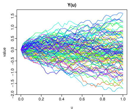
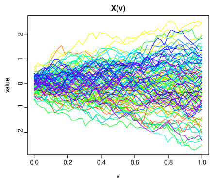
Figure 1: Functional time series plots of the generated functional response $\mathcal{Y}_{1}(u)$, …, $\mathcal{Y}_{n}(u)$, and functional predictor $\mathcal{X}_{1}(v)$, …, $\mathcal{X}_{n}(v)$.

Throughout the experiments, $n=[250,500,1000]$ functions are generated at $p$ equally spaced points in the interval $u,v\in[0,1]$. For each sample size, the generated data are divided into the training and test samples with sizes $0.8\times n$ and $0.2\times n$, respectively. Using the first $0.8\times n$ of the data, we obtained one-step-ahead forecasts of $\mathcal{X}_{t}(v)$ and $\mathcal{Y}_{t}(u)$ at time $t=0.8\times n+1$. Having increased the training sample by one, we then obtain-one step-ahead forecasts of $\mathcal{X}_{t}(v)$ and $\mathcal{Y}_{t}(u)$ at time $t=0.8\times n+2$. This process is repeated until the training sample covers the entire data. For each sample size, we repeat this procedure 100 times and for each time, we compute the GcGMC values of the predictor and response variables. If GcGMC($\mathcal{Y}$) $>$ GcGMC($\mathcal{X}$), we conclude $\mathcal{Y}$ is more predictable than $\mathcal{X}$. Further, if GcGMC($\mathcal{Y})>0$ and GcGMC($\mathcal{X})<0$, we conclude that $\mathcal{X}$ Granger-causes $\mathcal{Y}$, and thus $\mathcal{X}$ is more adequate to be the predictor. In Table 1, we report the number of times, where GcGMC($\mathcal{Y}$) $>$ GcGMC($\mathcal{X}$) and GcGMC($\mathcal{Y})>0$, GcGMC($\mathcal{X})<0$. As sample size $n$ increases from 250 to 1000, the probability of making a correct decision increases.

Table 1: Out of 100 replications, we compute the number of times where $\mathcal{Y}$ is more predictable than $\mathcal{X}$ when GcGMC($\mathcal{Y}$) $>$ GcGMC($\mathcal{X}$) and $\mathcal{X}$ Granger-causes $\mathcal{Y}$ when GcGMC($\mathcal{Y})>0$ and GcGMC($\mathcal{X})<0$.

	GcGMC($\mathcal{Y}$) $>$ GcGMC($\mathcal{X}$)			GcGMC($\mathcal{Y})>0$, GcGMC($\mathcal{X})<0$
$p\backslash n$	250	500	1000	250	500	1000
50	88	94	99	57	84	92
100	90	99	100	62	82	96
200	91	97	99	74	81	90
400	96	99	99	71	85	92

5 Data analyses

5.1 Sea surface temperature and sea-level atmospheric pressure

The Oceanic Niño index (ONI) is one of the primary indices used to monitor the El Niño Southern Oscillation. The National Oceanic and Atmospheric Administration (https://www.noaa.gov) agency considers El Niño conditions to be present when the ONI is +0.5 or higher, indicating the east-central tropical Pacific is significantly warmer than usual. La Niña conditions exist when the ONI is -0.5 or lower, indicating the region is cooler than usual. The ONI is computed by averaging 3-month sea surface temperature anomalies in an area of the east-central equatorial Pacific ocean, called the Niño 3.4 region (5S to 5N; 170W to 120W). The 3-month running average of sea surface temperature is often compared to a 30-year average as an indicator of the climate becoming warmer or cooler.

The Southern Oscillation Index (SOI) is a measure of the strength of the Walker circulation. It is a critical atmospheric index for controlling the strength of El Niño and La Niña events. The SOI measures the difference in sea-level atmospheric pressure between Tahiti and Darwin, Australia. By standardizing sea-level atmospheric pressures in Tahiti and Darwin, the SOI is obtained by a ratio between the difference of the two standardized sea-level atmospheric pressures and their normalized standard deviation.

We consider the bivariate curve time series for the monthly sea surface temperature and sea-level atmospheric pressure from January 1951 to December 2018. The data sets can be obtained from https://www.cpc.ncep.noaa.gov/data/indices/soi and https://www.cpc.ncep.noaa.gov/products/analysis_monitoring/ensostuff/detrend.nino34.ascii.txt. In Figure 2, we plot the two functional time series.

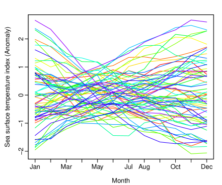
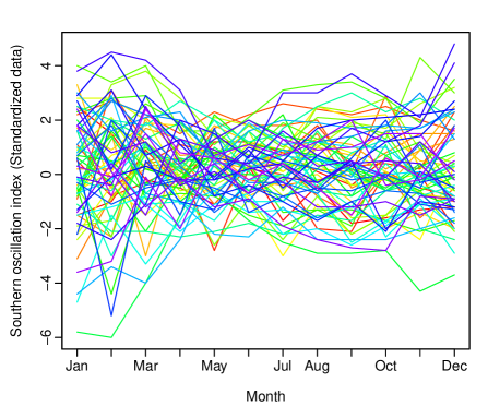
Figure 2: Functional time series plots of the sea surface temperature anomaly and southern oscillation index (a standardized measure of sea-level atmospheric pressure) observed from January 1951 to December 2018. Each curve represents data in a year.

We implement a functional nonparametric regression to predict the sea-level atmospheric pressure and sea surface temperature. We split our entire sample into an initial training sample consisting of years from 1951 to 1983 and a testing sample composed of years from 1984 to 2018. Using the years from 1951 to 1983, we obtain one-step-ahead forecasts of the sea-level atmospheric pressure and sea surface temperature in 1984. Then, we increase the training sample by one year and obtain one-step-ahead forecasts of the sea-level atmospheric pressure and sea surface temperature in 1985, respectively. We obtain our forecasts through this expanding window approach until the training sample covers the entire data sample.

Let $\mathcal{X}$ be the sea-level atmospheric pressure, and $\mathcal{Y}$ be the sea surface temperature. With the 35 years of forecasts and their corresponding forecast errors, we compute the GcGMC values of (6) and (7), namely GcGMC$(\mathcal{X})=0.0093$ and GcGMC$(\mathcal{Y})=-0.2441$. Given $\text{GcGMC}(\mathcal{X})>\text{GcGMC}(\mathcal{Y})$, we conclude $\mathcal{X}$ is more predictable than $\mathcal{Y}$. Because the GcGMC of the sea-level atmospheric pressure is greater than 0, the inclusion of the sea surface temperature can help to reduce the sum squared prediction errors in the prediction of the sea-level atmospheric pressure. Because the GcGMC of the sea surface temperature is less than 0, the inclusion of the sea-level atmospheric pressure cannot help to reduce the sum squared prediction errors in the prediction of the sea surface temperature. Therefore, we conclude that the sea surface temperature Granger-causes the sea-level atmospheric pressure.

5.2 Dow-Jones Industrial Average and its constituent stocks

The Dow-Jones Industrial Average (DJIA) is a stock market index that shows how 30 large publicly owned companies based in the United States have traded during a standard New York Stock Exchange trading session. We consider daily cross-sectional returns from 2/January/2018 to 31/December/2018. The data were obtained from the Thompson Reuters DataScope Tick History. We have a sample of log-price observations, denoted by $q_{t}^{j}(u_{i})$ for each day $t=1,\dots,n$. We define the $j$^th log return on day $t$ as

$$r^{j}_{t}(u_{i})=q_{t}^{j}(u_{i+1})-q_{t}^{j}(u_{i}),\qquad i=1,\dots,95,$$

that is, $r^{j}_{t}(u_{i})$ is the log return for $j$^th company at the middle of time interval $i$ at day $t$ (e.g., see Kokoszka et al., 2017; Shang et al., 2019; Li et al., 2020). In a given day, there are 96 5-minute price observations from 9:30 to 17:20 Eastern time, resulting in 95 values of the log returns.

In Table 2, we list 30 constituent stocks of the DJIA. There are five stocks, namely Cisco, Dow Chemical, Intel, Microsoft, and Walgreen, that have missing observations, and are thus removed from our analysis for consistency.

Table 2: Stock name and tick symbol of 30 constituent of the Dow-Jones index

Stock	Tick symbol	Stock	Tick symbol	Stock	Tick symbol
Apple Inc	AAPL.OQ	IBM	IBM	PFE	Pfizer
AXP	American Express	INTC.OQ	Intel	PG	Procter & Gamble
BA	Boeing	JNJ	Johnson & Johnson	TRV	Travelers Companies Inc
CAT	Caterpillar	JPM	JPMorgan Chase	UNH	United Health
CSCO.OQ	Cisco	KO	Coca-Cola	UTX	United Technologies
CVX	Chevron	MCD	McDonald’s	V	Visa
DIS	Disney	MMM	3M	VZ	Verizon
DOW	Dow Chemical	MRK	Merck	WBA.OQ	Walgreen
GS	Goldman Sachs	MSFT.OQ	Microsoft	WMT	Wal-Mart
HD	Home Depot	NKE	Nike	XOM	Exxon Mobil

We implement a functional nonparametric regression to predict the DJIA, and each of the 25 stocks. We split our entire sample into an initial training sample consisting of days from 2/January/2018 to 7/August/2018 (151 days in total) and a testing sample composed of days 8/August/2018 to 31/December/2018 (100 days in total). Using days from 2/January/2018 to 7/August/2018, we obtain one-step-ahead forecasts of the DJIA and each of its constituent stocks on day 8/August/2018. Then, we increase the training sample by one day and obtain one-step-ahead forecasts of the DJIA and each of its constituent stock in day 9/August/2008, respectively. Through this expanding-window approach, we obtain our forecasts until the training sample covers the entire data sample.

With 100 days of forecasts and their corresponding forecast errors, we compute the GcGMC values when either a stock or DJIA is a response variable in the nonparametric function-on-function regression in Table 3. Let $\mathcal{X}$ be the log-return of DJIA and $\mathcal{Y}$ be the log-return of a stock. For several stocks highlighted in blue in the table, we observe that the GcGMC of the DJIA is less than 0, and the GcGMC of the stock is greater than 0. Thus, the DJIA’s inclusion can help reduce the sum squared prediction errors in the stock’s prediction. These stocks highlighted in blue are lagging behind the DJIA for the period we considered. When the two GcGMC values have the same sign, we can no longer make a specific statement about leading and lagging. Instead, we can only highlight those stocks that are less predictive than the DJIA in red as GcGMC$(\mathcal{X})$ $>$ GcGMC$(\mathcal{Y})$; similarly, those stocks that are more predictive than the DJIA in white. For those stocks that are lagging behind the DJIA, a possible practical implication is to predict the direction of their log returns based on the most recent log return of the DJIA.

Table 3: GcGMC values when either the log return of a stock or DJIA is the response variable in the nonparametric function-on-function regression.

Variable	GcGMC	Variable	GcGMC	Variable	GcGMC	Variable	GcGMC	Variable	GcGMC
AAPL.OQ	0.0031	AXP	0.0058	JNJ	0.0039	KO	0.0006	MRK	0.0032
DJIA	-0.0185	DJIA	-0.0063	DJIA	-0.0064	DJIA	-0.0055	DJIA	-0.0201
NKE	0.0015	PFE	0.0013	UNH	0.0019	UTX	0.0031	WMT	0.0007
DJIA	-0.0133	DJIA	-0.0140	DJIA	-0.0087	DJIA	-0.0127	DJIA	-0.0061
TRV	-0.6959	BA	-0.0022	CAT	-0.0040	CVX	-0.0014	DIS	-0.0001
DJIA	-0.0107	DJIA	-0.0125	DJIA	-0.0091	DJIA	-0.0062	DJIA	-0.0046
GS	-0.0034	HD	-0.0031	IBM	0.0047	JPM	-0.0046	MCD	-0.0003
DJIA	-0.0121	DJIA	-0.0073	DJIA	0.0141	DJIA	-0.0052	DJIA	-0.0107
MMM	-0.0015	PG	-0.0071	V	-0.0011	VZ	-0.0051	XOM	-0.0004
DJIA	-0.0102	DJIA	-0.0079	DJIA	-0.0024	DJIA	-0.0132	DJIA	-0.0074

5.3 S&P 500 index and WTI oil price

The S&P 500 index is a stock market price representing the performance of around 500 of the largest U.S. companies. When observing the S&P 500 index, we also observe oil prices from West Texas Intermediate (WTI). We aim to investigate if the oil price is a leading or lagging variable of the S&P 500. We collected monthly S&P 500 indexes and WTI prices from January/1984 to December/2019 (432 months in total). For each month in a given year $t$, we compute the normalized prices of the S&P 500 and WTI by taking into account the consumer price index in the United States (CPI). The normalized prices can be expressed as

$$q_{t}^{\text{WTI}}(u_{i}) =\frac{\text{WTI}_{\text{observed},t}(u_{i})}{\text{CPI}_{\text{observed},t}(u_{i})}\times 100,$$

$$q_{t}^{\text{S\&P 500}}(u_{i}) =\frac{\text{S\&P 500}_{\text{observed},t}(u_{i})}{\text{CPI}_{\text{observed},t}(u_{i})}\times 100,$$

where $i$ denotes any given month. The log returns of the normalized WTI and S&P 500 at month $i$ in year $t$ can be expressed as

$$r_{t}^{\text{WTI}}(u_{i}) =\ln\left[\frac{q_{t}^{\text{WTI}}(u_{i+1})}{q_{t}^{\text{WTI}}(u_{i})}\right],$$

$$r_{t}^{\text{S\&P 500}}(u_{i}) =\ln\left[\frac{q_{t}^{\text{S\&P 500}}(u_{i+1})}{q_{t}^{\text{S\&P 500}}(u_{i})}\right],\qquad i=1,\dots,11.$$

In Figure 3, we display two functional time series plots of the log returns of the S&P 500 and WTI. Using a stationarity test of Horváth et al. (2014), we checked and verified that both series are stationary with $p$-values of 0.998 and 0.931, respectively.

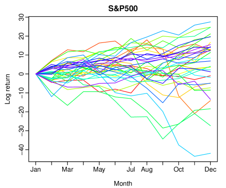
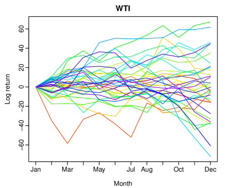
Figure 3: Functional time series plots of the log returns of the normalized prices of the S&P 500 and WTI by incorporating the consumer price index in the United States.

We implement a nonparametric function-on-function regression to predict the log returns of S&P 500 and WTI. The entire data set was split into an initial training sample consisting of monthly log returns from January/1984 to December/2003 (20 curves in total) and a testing sample composed of months from January/2004 to December/2019 (16 curves in total). Using the initial training sample, we obtain one-step-ahead curve forecasts of the log returns of the WTI and S&P 500 in 2004. Then, we increase the number of curves in the training sample by one year and obtain one-step-ahead forecasts of the WTI and S&P 500 in 2005. Through an expanding-window approach, we obtain our forecasts until the training sample covers the entire data sample.

Let $\mathcal{X}$ be the S&P 500 log returns and $\mathcal{Y}$ be the WTI log returns. With 16 curves in the testing sample, we compute the corresponding one-step-ahead forecast errors, from which we compute the GcGMC when the S&P 500 or WTI is the response variable, namely GcGMC$(\mathcal{X})=-0.0232$ and GcGMC$(\mathcal{Y})=0.1255$. We observe that the GcGMC of the WTI is greater than 0, and the GcGMC of the S&P 500 is less than 0, so the inclusion of the S&P 500 can help reduce the sum squared prediction errors in the prediction of the WTI. Thus, the S&P 500 index is a leading variable of the WTI price. A possible practical implication is to predict the direction of the WTI price based on the most recent S&P 500 index.

6 Conclusion

We extend the Granger causality generalized measures of correlation from bivariate scalar to curve time series. With this measure, we can investigate which curve time series Granger-causes the other one; in turn, it helps to determine suitable predictor and response variables. Granger causality can be viewed from a prediction viewpoint. The measure can be computed by a nonparametric function-on-function regression that captures the possible nonlinear pattern between the predictor and response. Illustrated by a climatology data set, we find that the sea surface temperature Granger-causes the sea-level atmospheric pressure. From the Dow-Jones index data set, we find those constituent stocks that are lagged behind the Dow-Jones index. From the S&P 500 and WTI oil data sets, we find that the S&P 500 index Granger causes the WTI price.

There are two limitations associated with our Granger causality generalized measures of correlation. This measure depends on the length of training and testing samples. Sometimes, an outlying observation in the testing sample can affect the estimation accuracy of our proposed measure. Second, we compute a one-step-ahead forecast and its errors as a way of assessing predictive ability. While this sets up the foundation for our measure, it is sometimes more useful to consider other longer-term forecast horizons.

There are several ways in which the current work may be further extended, and we briefly outline three. First, we could extend Granger causality tests studied in Geweke (1984) to function-valued variables, and possibly assess the strength of this relationship (see, e.g., Taamouti et al., 2014). Second, since there is a strong connection between Granger causality and co-integration (see, e.g., Granger, 1986, 1988), one may study the concept of co-integration in non-stationary functional time series. Finally, the causality arisen from the Granger causality generalised measures of correlation may depend on a specific forecast horizon. We may extend the current work by forecasting $h>1$ step ahead, which may help to incorporate seasonality in a functional time series forecasting (see, e.g., Chen et al., 2019).

References

- (1)
- Allen & Hooper (2018) Allen, D. E. & Hooper, V. (2018), ‘Generalized correlation measures of causality and forecasts of the VIX using non-linear models’, Sustainability 10(8), 2695.
- Chen et al. (2017) Chen, M., Lian, Y. M., Chen, Z. & Zhang, Z. (2017), ‘Sure explained variability and independence screening’, Journal of Nonparametric Statistics 29(4), 849–883.
- Chen et al. (2019) Chen, Y., Marron, J. S. & Zhang, J. (2019), ‘Modeling seasonal and serial dependence of electricity price curves with warping functional autoregressive dynamics’, The Annals of Applied Statistics 13(3), 1590–1616.
- Diks & Panchenko (2006) Diks, C. & Panchenko, V. (2006), ‘A new statistic and practical guideline for nonparametric Granger causality testing’, Journal of Economic Dynamics and Control 30(9-10), 1647–1669.
- Ferraty & Vieu (2006) Ferraty, F. & Vieu, P. (2006), Nonparametric Functional Data Analysis, Springer, New York.
- Geweke (1984) Geweke, J. (1984), Inference and causality in economic time series models, in Z. Griliches & M. D. Intriligator, eds, ‘Handbook of Econometrics II’, North-Holland, Amsterdam, chapter 19.
- Granger (1969) Granger, C. W. J. (1969), ‘Investigating causal relations by econometric models and cross-spectral methods’, Econometrica 37(3), 424–438.
- Granger (1980) Granger, C. W. J. (1980), ‘Testing for causality: A personal viewpoint’, Journal of Economic Dynamics and Control 2, 329–352.
- Granger (1986) Granger, C. W. J. (1986), ‘Developments in the study of co-integrated economic variables’, Oxford Bulletin of Economics and Statistics 48(3), 213–228.
- Granger (1988) Granger, C. W. J. (1988), ‘Some recent developments in a concept of causality’, Journal of Econometrics 39(1-2), 199–211.
- Granger & Thomson (1987) Granger, C. W. J. & Thomson, P. J. (1987), ‘Predictive consequences of using conditioning or causal variables’, Econometric Theory 3(1), 150–152.
- Hiemstra & Jones (1994) Hiemstra, C. & Jones, J. D. (1994), ‘Testing for linear and nonlinear Granger causality in the stock price-volume relation’, The Journal of Finance 49(5), 1639–1664.
- Horváth & Kokoszka (2012) Horváth, L. & Kokoszka, P. (2012), Inference for Functional Data with Applications, Springer, New York.
- Horváth et al. (2014) Horváth, L., Kokoszka, P. & Rice, G. (2014), ‘Testing stationarity of functional time series’, Journal of Econometrics 179(1), 66–82.
- Kokoszka & Reimherr (2017) Kokoszka, P. & Reimherr, M. (2017), Introduction to Functional Data Analysis, CRC Press, Boca Raton.
- Kokoszka et al. (2017) Kokoszka, P., Rice, G. & Shang, H. L. (2017), ‘Inference for the autocovariance of a functional time series under conditional heteroscedasticity’, Journal of Multivariate Analysis 162, 32–50.
- Li et al. (2020) Li, D., Robinson, P. M. & Shang, H. L. (2020), ‘Long-range dependent curve time series’, Journal of the American Statistical Association: Theory and Methods 115(530), 957–971.
-
R Core Team (2020)
R Core Team (2020), R: A Language and
Environment for Statistical Computing, R Foundation for Statistical
Computing, Vienna, Austria.
https://www.R-project.org/ - Seth et al. (2015) Seth, A. K., Barrett, A. B. & Barnett, L. (2015), ‘Granger causality analysis in neuroscience and neuroimaging’, The Journal of Neuroscience 35(8), 3293–3297.
- Shang (2017) Shang, H. L. (2017), ‘Functional time series forecasting with dynamic updating: An application to intraday particulate matter concentration’, Econometrics and Statistics 1, 184–200.
- Shang et al. (2019) Shang, H. L., Yang, Y. & Kearney, F. (2019), ‘Intraday forecasts of a volatility index: Functional time series methods with dynamic updating’, Annals of Operations Research 282(1), 331–354.
- Taamouti et al. (2014) Taamouti, A., Bouezmarni, T. & El Ghouch, A. (2014), ‘Nonparametric estimation and inference for conditional density based Granger causality measures’, Journal of Econometrics 180, 251–264.
- Vinod (2017) Vinod, H. D. (2017), ‘Generalized correlation and kernel causality with applications in development economics’, Communications in Statistics – Simulation and Computation 46(6), 4513–4534.
-
Vinod (2019)
Vinod, H. D. (2019), generalCorr:
Generalized Correlations and Plausible Causal Paths.
R package version 1.1.5.
https://CRAN.R-project.org/package=generalCorr - Wiener (1956) Wiener, N. (1956), The theory of prediction, in E. F. Beckenback, ed., ‘Modern Mathematics for Engineers’, McGraw-Hill, New York.
- Zheng et al. (2012) Zheng, S., Shi, N.-Z. & Zhang, Z. (2012), ‘Generalized measures of correlation for asymmetry, nonlinearity, and beyond’, Journal of the American Statistical Association: Theory and Methods 107(499), 1239–1252.