Assessing the foundation and applicability of some dark energy fluid models in the Dirac-Born-Infeld framework

Abstract

In this paper, we will deepen the understanding of some fluid models proposed by other authors for the description of dark energy. Specifically, we will show that the so-called (Modified) Berthelot fluid is the hydrodynamic realization of the free Dirac-Born-Infeld theory and that the Dieterici fluid admits a non-relativistic $k$-essence formulation; for the former model the evolution of the scalar field will be written in terms of some cosmographic parameters. The latter model will also be tested using Machine Learning algorithms with respect to cosmic chronometers data, and results about the dynamics at a background level will be compared with those arising when other fluids (Generalized Chaplygin Gas and Anton-Schmidt) are considered. Due to some cosmic opacity effects, the background cosmology of universes filled by these inequivalent fluids, as they arise in physically different theories, may not be enough for discriminating among them. Thus, a perturbation analysis in the long-wavelength limit is carried out revealing a rich variety of possible behaviors. It will also be shown that the free Dirac-Born-Infeld theory cannot account for flat galactic rotation curves, and therefore we derive an appropriate relationship between the scalar field potential and the brane tension for achieving this goal; this provides an estimate for the dark matter adiabatic speed of sound inside the halo consistent with other literature. A certain relationship between the Newtonian gravitational potential within the galaxy and the Lagrangian potential in the non-relativistic regime for the (Modified) Berthelot fluid will also be enlightened.

I Introduction

The existence of a dark energy fluid has been claimed for accounting for the accelerated expansion of the Universe sup1 ; sup2 . Its existence is compatible also with the theoretical description of the cosmic microwave background cmb1 ; cmb2 , the baryon acoustic oscillation (BAO) spectra bao1 ; bao2 , and the cosmic evolution HZ2 ; HZ3 . The minimal proposal for the modelling of dark energy, the cosmological constant, is mathematically consistent with the symmetries of general relativity, but this approach would violate the causality principle, should we interpret the cosmological constant as a fluid with $p=-\rho$ Ref1 . On the other hand, astrophysical observations suggest that our Universe should also be filled with dark matter, which can be macroscopically pictured as pressureless dust, regardless of its elementary particle foundation in terms of either massive neutrinos, sterile neutrinos, axions, axinos, gravitinos, or neutralinos Ref2 ; Ref3 ; Ref4 ; Ref5 ; Ref6 ; Ref7 ; Ref8 (see, e.g., annrev for a review of different candidates of dark matter particles). Some amount of non-baryonic matter is needed to account for the rotation curves of galaxies and to address the problem of the formation of astrophysical structures. In fact, a local collapse of cosmic material requires dark matter to dominate over dark energy in the past cosmological epochs, as it can be seen in the behavior of the spectrum of mass fluctuations at short wavelengths (see bertone and references therein).

The Generalized Chaplygin Gas is a very successful proposal for a unified description of these two cosmic fluids, and it comes with the good features of restoring causality and predicting a transition from an epoch dominated by dark matter to a subsequent one dominated by dark energy. This permits us to account for the existence of astrophysical structures inside an accelerated expanding Universe, and the sturdiness of this paradigm has been confirmed by a large number of model testing investigations, as summarized in chapI ; Sergei . Furthermore, it has been discovered that the Generalized Chaplygin Gas is not only an ad-hoc phenomenological framework because it arises also from the Nambu-Goto theory with soft corrections (i.e. logarithmic in the kinetic energy of the scalar field) for the dynamics of a 2-dimensional brane gene1 , and the properties of its symmetry group have been widely discussed jackiw . Nevertheless, also the Dieterici fluid can realize a dark matter-dark energy phase transition dieterici1 ; dieterici2 , whose quantitative predictions with respect to cosmic chronometers data will be assessed in this paper. The reason is that a series expansion in the energy density of the Dieterici equation of state (EoS) may be constituted by Generalized-Chaplygin-Gas-like addenda, making the analysis whether the Nature favours exactly one of those terms, like in a Generalized Chaplygin Gas, or their summation, of crucial importance. Here we will show that the redshift evolution of the Hubble rate does not necessarily call for an extension of the Generalized Chaplygin Gas into a Dieterici fluid; the data points describing the cosmic history were obtained by applying the differential age method, and the reader can find them reported in zhang2016 . This technique allows estimating the time derivative of the redshift through the measurements of the different ages of passively-evolving galaxies at different redshifts, which is then used to determine the values of the cosmological parameters, like the Hubble constant and the EoS of the cosmic fluid jimenez . In our analysis, we will forecast the model-free parameters by applying recently developed Machine Learning (ML) algorithms in which we train a computer system to make predictions by recognizing the properties of the data themselves. In fact, our ML approach has already been proven to be a valuable technique for testing the dataset’s consistency, searching for new physics and tensions in the data, and placing tighter constraints on the theoretical parameters revmod . For example, they have been employed for taming systematics in the estimates of the masses of clusters, for discriminating between different gravity theories when looking at statistically similar weak lensing maps, in N-body simulations, cosmological parameters inference, dark energy model comparison, supernova classification, strong lensing probes, and it is expected that they will be useful for the next generation of CMB experiments, (see revmod for a report about the state of the art applications of ML approaches over many different branches of Physics).

Another fluid model which has already been tested as a dark energy candidate is the so-called (Modified) Berthelot fluid capo . While being originally proposed for a realistic description of the fugacity properties of hydrocarbons reos2 , it has received novel attention in recent cosmological applications for example in interacting dark matter - dark energy scenarios in which, in particular, the avoidance of specific cosmological singularities has been assessed epjc2020 , in black hole cosmic accretion phenomena in the McVittie framework mcvittie , and in early-late time unification in quadratic gravity saikat . In this paper, we will provide a transparent foundation of this hydrodynamical model by reconstructing its relationship to the Dirac-Born-Infeld theory. We will as well reconstruct the $k$-essence formulation of the aforementioned Dieterici fluid in the non-relativistic regime, which would then be compared with those of the Generalized Chaplygin Gas and of the Anton-Schmidt fluid, which instead belong to the family of the Generalized Born-Infeld theories poin ; avelino . We refer also to cheva for the construction of the k-essence formulation for barotropic, logotropic and Bose-Einstein condensates fluid models. Exploiting the relationship between (Modified) Berthelot fluid and free Dirac-Born-Infeld theory we will show that this paradigm is challenged by astrophysical requirements of flat galactic rotation curves: this will call us to derive an appropriate relationship between scalar field potential and brane tension.

Unfortunately, investigating the dynamics at a background level for these fluids is not enough for concluding which one is the physical theory behind dark energy. A further source of uncertainty comes from possible scattering effects between the photons constituting the light rays, whose detection constitutes a primary way of testing a certain cosmological model, and the interstellar medium. This phenomenon is accounted for by introducing a cosmic opacity function that acts as a scaling for the luminosity function. A plethora of different redshift parametrizations for the cosmic opacity has been constructed and investigated Lee . While a non perfectly transparent universe can be a solution to some of the current observational tensions, as small and large scale estimates of the Hubble constant PyMC3_p2 , this would somehow hide the properties of dark energy, and models based on different fluid pictures may become statistically indistinguishable at the background level. Therefore, for breaking this degeneracy, we will perform a mathematical analysis of the evolution of perturbations in the long-wavelength limit for epochs in which dark energy dominates over dark matter assuming small deviations from the ideal fluid behavior in which pressure and energy density would be proportional to each other. We will find a rich variety of behaviors for the different fluid models either exhibiting time increasing or decreasing density contrasts and with or without oscillations; we will be able to provide as well some analytical solutions in a closed form which can serve as a valuable tool for comparison with similar analysis concerning further dark energy models that future literature may come up with.

Our paper is organized as follows: In Sect.II, we introduce the dynamical equations at a background level for the cosmological models we are interested in, deriving a novel non-relativistic $k$-essence formulation for the Dieterici fluid and proposing a connection between the (Modified) Berthelot fluid and the Dirac-Born-Infeld paradigm for deepening the understanding of the meaning of the free parameters beyond the thermodynamical fluid approach. In Sect.III, we will first review the foundation of the specific Bayesian Machine Learning (BML) method we will apply explaining its suitability for our analysis, and then we will forecast the free parameters of the model based on the Dieterici fluid also validating our results by comparing with observational data. Some degeneracy between physically different (e.g., arising in different frameworks as the Dirac-Born-Infeld vs. the Generalized Born Infeld) descriptions of dark energy will be mentioned in light of cosmic opacity effects in Sect.IV.1. This will call for the study of the evolution of density perturbations beyond the background level, whose results in the long-wavelength limit will be exhibited in Sect.IV.2 for different modelings of the cosmic fluid. In Sect.V we will assess the applicability of the models with respect to flat galactic rotation curves first pointing out and then resolving some shortcomings of the free Dirac-Born-Infeld model. Finally, we will comment on the cosmological meaning of our results and conclude in Sect.VI.

II Background field equations

The dynamics at the background level of the Hubble function $H$, and of the energy densities of cold dark matter and dark energy in a flat homogeneous and isotropic universe is governed by the evolution equations peebles :

$$H^{2}\,=\,\frac{\rho+\rho_{dm}}{3}\,,\qquad\dot{\rho}\,=\,-3H(\rho+p)\,,\qquad\dot{\rho}_{dm}\,=\,-3H\rho_{dm}\,,$$ (1)

where an over dot stands for a derivative with respect to the cosmic time. For avoiding loss of generality and accounting for the observational properties of the matter power spectrum zalda , we will assume that the dark matter abundance is quantified either by $\rho_{dm}$, and by some unified form of dark matter - dark energy in which pressure and energy density are related to each other according to equations of state of the form $p=w(\rho)\rho$. In particular, we want here to establish the field theory foundation of two fluid models previously proposed by some other authors just at the hydrodynamical level and known under the name of Dieterici model dieterici1 ; dieterici2

$$p=A\rho e^{B\rho}\,,$$ (2)

and of (Modified) Berthelot fluid capo ; reos2

$$p=\frac{B\rho}{1+A\rho}\,,$$ (3)

with $A$ and $B$ being free parameters.

II.1 Field theory formulation of the Dieterici fluid

The Dieterici equation of state (2) reduces to the Van der Waals model for imperfect fluid at low energy density dieterici3 ; dieterici4 ; dieterici5 . The physical idea at the core of this model is to incorporate the attractive and repulsive contributions to the pressure as

$$P=P_{\rm repulsive}e^{-P_{\rm attractive}}\,,$$ (4)

rather than

$$P=P_{\rm repulsive}+P_{\rm attractive}\,,$$ (5)

for getting more realistic estimates of the value of the critical compressibility factor dietericiaip . We are interested in this particular fluid model because it can interpolate between pressureless dust at high densities and a form of dark energy in the opposite regime, as it can be appreciated by looking at its effective equation of state parameter

$$w:=\frac{p}{\rho}=Ae^{B\rho}\,,$$ (6)

if we choose negative values for the free parameters $A$ and $B$ dieterici1 ; dieterici2 . We exhibit in Fig. 1 a comparison between the effective EoS parameter $w$ for the Dieterici fluid and the Generalized Chaplygin Gas (the latter fluid is characterized by $p=-{A}/{\rho^{B}}$). The degeneracy between the two models at the level of the effective EoS parameter is qualitatively noteworthy. In this paper, we will discriminate quantitatively between the two models.

$\begin{array}[]{cccc}\includegraphics[width=213.39566pt]{eos1.pdf}&&\includegraphics[width=213.39566pt]{eos2.pdf}\\ \end{array}$

Figure 1: The figure displays the comparison between the effective EoS parameter $w={p}/\rho$ of the Dieterici fluid (left panel) and of the Generalized Chaplygin Gas (right panel). In the former case we have fixed $A=-12.0$ and $B=-7.0$ (yellow curve), $B=-8.0$ (red curve), $B=-9.0$ (black curve), and $B=-10.0$ (green curve), while in the latter we have fixed $A=0.02$ and $B=1.0$ (yellow curve), $B=1.5$ (red curve), $B=2.0$ (black curve), and $B=2.5$ (green curve). Both fluid models interpolate between pressureless dust at high energy density, and a form of dark energy in the opposite regime, and their qualitative similarity is noteworthy.

The adiabatic speed of sound squared for the Dieterici fluid (2) is given by

$$c_{s}^{2}:=\frac{\partial p}{\partial\rho}=A(B\rho+1)e^{B\rho}\,,$$ (7)

which, for negative $A$ and $B$, is positive in the energy density range $\rho<-1/B$. We remark that outside this range, the model can still be stable under small-wavelength perturbations as explained in corr2 .

The cosmological relevance of Dieterici fluids can be better appreciated by formulating the model through a $k$-essence Lagrangian which thus is a function only of the kinetic energy of an underlying scalar field. An exact analytical result can be found in the non-relativistic regime, which can also open a path to the construction of the related Poincaré algebra poin and allows for a transparent comparison with some other fluid approaches applied for the dark matter - dark energy unification in previous literature, namely the Generalized Chaplygin Gas and the Logotropic model. We recall that in the canonical formalism, the Lagrangian should be computed via the pressure pres1 ; pres2 ; pres3 :

$${\mathscr{L}}=p\,.$$ (8)

Introducing the scalar field $\theta$ which is canonically conjugate to $\rho$, i.e. their Poisson bracket reads as $\{\theta(x_{i}),\,\rho(x_{j})\}=\delta(x_{i}-x_{j})$, the Lagrangian can be recast as

$${\mathscr{L}}(\rho,\dot{\rho},t,x^{i})=\dot{\rho}\theta-\frac{1}{2}\rho\partial_{i}\theta\partial^{i}\theta-V(\rho)\,.$$ (9)

The potential for an irrotational fluid should be reconstructed by solving potpres :

$$p=\rho\frac{dV(\rho)}{d\rho}-V(\rho)\,,$$ (10)

which, for a Dieterici fluid with $p=A\rho e^{B\rho}$, delivers

$$V(\rho)=-A\rho{\rm Ei}(-B\rho)\,,$$ (11)

where the constant of integration has been fixed by imposing $V(0)=0$, and where ${\rm Ei}$ denotes the exponential integral. Thus:

$$\frac{dV(\rho)}{d\rho}=A(e^{B\rho}-{\rm Ei}(-B\rho)).$$ (12)

Next, the value of $\rho$ should be found by solving the Euler-Lagrange equation of motion

$$\dot{\theta}=-\frac{1}{2}\partial_{i}\theta\partial^{i}\theta-\frac{dV(\rho)}{d\rho}\,.$$ (13)

We will solve this equation of motion in the two limiting regimes of low and high energies which correspond to dark energy and dark matter dominated epochs. We obtain:

$$\frac{dV(\rho)}{d\rho}\Big{|}_{\rho<<1}\simeq A(1+\gamma+\ln(-B\rho))+2AB\rho\quad\Rightarrow\quad\rho=\frac{1}{2B}W\left(-2{\rm Exp}\left(-\frac{\dot{\theta}+\frac{1}{2}\partial_{i}\theta\partial^{i}\theta}{A}-(1+\gamma)\right)\right)\,,$$ (14)

$$\frac{dV(\rho)}{d\rho}\Big{|}_{\rho>>1}\simeq Ae^{B\rho}\quad\Rightarrow\quad\rho=\frac{1}{B}\ln\left[-\frac{1}{A}\left(\dot{\theta}+\frac{1}{2}\partial_{i}\theta\partial^{i}\theta\right)\right]\,.$$ (15)

Implementing these results into (8) by using the Dieterici equation of state we get:

$${\mathscr{L}}\simeq\left[-W\left(-2{\rm Exp}\left(-\frac{\dot{\theta}+\frac{1}{2}\partial_{i}\theta\partial^{i}\theta}{A}-(1+\gamma)\right)\right){\rm Exp}\left(-\frac{1}{A}\left(\dot{\theta}+\frac{1}{2}\partial_{i}\theta\partial^{i}\theta\right)-(1+\gamma)\right)\right]^{\rm 1/2}\quad{\rm for}\quad{\rho<<1}\,,$$ (16)

$${\mathscr{L}}\simeq\left(\dot{\theta}+\frac{1}{2}\partial_{i}\theta\partial^{i}\theta\right)\ln\left(-\frac{\dot{\theta}+\frac{1}{2}\partial_{i}\theta\partial^{i}\theta}{A}\right)\quad{\rm for}\quad{\rho>>1}\,,$$ (17)

where we have also taken into account that Lagrangians that differ by a multiplicative constant are physically equivalent (that is, they provide the same equations of motion). Our analysis shows that the parameter $B$, which quantifies the strength of the attractive effects between the fluid particles, does not affect the theory Lagrangian neither in the low energy limit nor in the high energy scenario. The physical meaning of the parameter $B$ has been provided in dou1 ; dou2 : we are considering a fluid formed by molecules that are interacting with each other. We assume that this attractive interaction force is experienced only by molecules close to each other. Inside the gas, the mutual forces between the molecules balance each other, but this would not be any longer the case for the molecules in the proximity of the boundary, in which case we will have a net force. Applying an argument by Boltzmann, it is shown that this net force does not influence the distribution of the velocities of the molecules (i.e., the kinetic energy), but their spatial distribution (i.e., the density). Thus, $B$ is a measure of the work that should be done for moving the molecules towards the boundary against this force field. Up to date, although a Lagrangian formulation has been proposed for the Generalized Chaplygin Gas, the physical meaning of its free parameters has not yet been clarified, unlike for the Dieterici model. Furthermore, from (15), we can understand that the functional form of the Dieterici equation of state leads to a shift in the derivative of the potential in the high energy scenario if compared to the logotropic framework luongo . In this latter paper results have been derived by means of Taylor expansions around certain values of the free model parameters, while in our case, the series expansions have been carried out with respect to the values of the energy density. Therefore, even though the Dieterici equation of state interpolates between dark matter and dark energy dominated epochs, as the Generalized Chaplygin Gas and the Logotropic model do (and they can be regarded as analogue proposals at the level of the effective fluid description), we can see that they deeply differ at the level of the underlying theory. In fact, in the former cases, the Lagrangian is monotonic with respect to the potential energy of the scalar field, while in the Dieterici case, non-monotonic behavior can be identified in (17) which represents the dark matter-dominated phase.

Dubbing $X=\dot{\theta}+\frac{1}{2}\partial_{i}\theta\partial^{i}\theta$ the kinetic energy, and expanding the Lagrangian (16) about $X=0$, we obtain at second order

$${\mathscr{L}}\simeq X+CX^{2}+o\left(X^{3}\right)\,,\qquad C=-\frac{s^{3}+5s^{2}+6s+4}{4\left(1+s\right)^{2}A\left(s+2\right)}\,,\qquad s=W\left(-2\mathrm{e}^{-(1+\gamma)}\right)\,,$$ (18)

where it should be emphasized that the deviations from linearity depends on the parameter $A$ only. Furthermore, in the regime characterized by (14) the Dieterici equation of state parameter (6) and the adiabatic speed of sound squared (7) as functions of the kinetic energy $X$ read as

$$w=A\left[-\frac{2\mathrm{e}^{-\left(\frac{X}{A}+(1+\gamma)\right)}}{W\left(-2\mathrm{e}^{-\left(\frac{X}{A}+(1+\gamma)\right)}\right)}\right]^{\frac{1}{2}}\,,\qquad c_{s}^{2}=\frac{w}{2}\left[2+W\left(-2\mathrm{e}^{-\frac{X}{A}-(1+\gamma)}\right)\right]\,,$$ (19)

from which we can compute

$$\frac{dc_{s}^{2}}{dX}=-\frac{y(4+y)}{4(1+y)}e^{\frac{y}{2}}\,,\qquad y=W(-2e^{-u})\,,\qquad u=\frac{X}{A}+1+\gamma\,.$$ (20)

Therefore, for understanding whether the adiabatic speed of sound within the Dieterici fluid is a monotonic function of the underlying scalar field kinetic energy, we need to establish whether the function

$$\tilde{s}=\frac{W(z)[4+W(z)]}{1+W(z)}$$ (21)

comes with a well-defined sign. We should note that $z=-2e^{-u}<0$, and that for a negative argument, the above quantity switches its sign in correspondence of the likewise property of $1+W(z)$. Thus, $c_{s}^{2}$ is not a monotonic function of $X$. We should also note that the approximation we are using here is applicable as long as $z>-1/e$ as by definition of Lambert function, which means as long as $X<A[\ln(1/2e)+1+\gamma]$.

On the other hand, by simple algebraic manipulations we get that the non-relativistic Lagrangian in (17) about $X=0$ is given by a softcore (e.g. logarithmic in the kinetic energy) correction to the linear regime:

$${\mathscr{L}}\simeq X\left[1-\frac{\ln(X)}{\ln|A|}\right]\,.$$ (22)

In the regime characterized by (15) the equation of state parameter and sound speed squared respectively read as

$$\omega=-X\,,\qquad c_{s}^{2}=-X\left[\ln\left(-\frac{X}{A}\right)+1\right]\,.$$ (23)

implying

$$\frac{dc_{s}^{2}}{dX}=-\left[\ln\left(-\frac{X}{A}\right)+2\right]\,.$$ (24)

Therefore, in this regime, the adiabatic speed of sound is a monotonic function of the kinetic energy of the scalar field, which is a physical property shared by the Generalized Born-Infeld model avelino . We should remark, however, that in the case of the Dieterici fluid, taking into account the discussion about (21), such a feature arises in the high energy regime only. This is an important difference between the physical foundations of the Generalized Chaplygin Gas and the Dieterici fluid, which was not self-evident by inspecting Fig. 1.

II.2 Field theory formulation of the (Modified) Berthelot fluid

We will now construct the underlying Lagrangian theory for the (Modified) Berthelot fluid (3) in both non-relativistic and relativistic regimes. We start by noticing that for this fluid the equation of state parameter and adiabatic speed of sound squared read respectively as

$$w=\frac{B}{1+A\rho}\,,\qquad c_{s}^{2}=\frac{\partial p}{\partial\rho}=\frac{B}{\left(1+A\rho\right)^{2}}\,.$$ (25)

II.2.1 Non-relativistic regime

In order to derive the non-relativistic Lagrangian formulation of which the (Modified) Berthelot fluid is the hydrodynamical realization, we follow again the classical formulation for an irrotational perfect fluid by introducing the potential V($\rho$) of the scalar field $\theta$. We reconstruct the potential by substituting (3) into (10)

$$V(\rho)=B\rho\ln\left({\frac{\rho}{A\rho+1}}\right),$$ (26)

where we have fixed the constant of integration by imposing $\lim_{\rho\to 0^{+}}V(\rho)=0$. When studying the rotation curves of galaxy we will enlighten a relationship between this Lagrangian potential and the Newtonian gravitational potential in (83). Next, by inserting

$$\frac{dV(\rho)}{d\rho}=B\ln\left(\frac{\rho}{A\rho+1}\right)+\frac{B}{A\rho+1}.$$ (27)

into (13) we can obtain the following relationship between fluid energy density and scalar field kinetic energy $X=\dot{\theta}+\frac{1}{2}\partial_{i}\theta\partial^{i}$:

$$\rho=-\frac{W\left[-A\operatorname{Exp}\left(-\frac{\dot{\theta}+\frac{1}{2}\partial_{i}\theta\partial^{i}\theta+B}{B}\right)\right]}{A\left(W\left[-A\operatorname{Exp}\left(-\frac{\dot{\theta}+\frac{1}{2}\partial_{i}\theta\partial^{i}\theta+B}{B}\right)\right]+1\right)}=-\frac{W\left[-A\operatorname{Exp}\left(-\frac{X+B}{B}\right)\right]}{A\left(W\left[-A\operatorname{Exp}\left(-\frac{X+B}{B}\right)\right]+1\right)}\,.$$ (28)

Now, plugging the above result into (8) we get for the (Modified) Berthelot equation of state (3):

$${\mathscr{L}}=W\left[-A\cdot{\rm Exp}\left(-\frac{\dot{\theta}+\frac{1}{2}\partial_{i}\theta\partial^{i}\theta+B}{B}\right)\right]=W\left[-A\cdot{\rm Exp}\left(-\frac{X+B}{B}\right)\right],$$ (29)

where again we have taken into account that Lagrangians differing by a multiplicative constant are physically equivalent because they provide the same Euler-Lagrange equations of motion. It should be noted that unlike in the Lagrangian formulation for the Dieterici fluid (16)-(17), in this case both the free model parameters $A$ and $B$ enter the expression for the Lagrangian. Expanding the Lagrangian we have just constructed about $X=0$ we get

$${\mathscr{L}}\simeq X+CX^{2}+o\left(X^{3}\right)\,,\qquad C=\frac{W\left(-A\mathrm{e}^{-1}\right)^{2}}{2\left(1+W\left(-A\mathrm{e}^{-1}\right)\right)^{4}B^{3}}\,,$$ (30)

which shows that the dependence on both the free parameters survives also in this limit. As from (25) the equation of state parameter and speed of sound squared are related to the scalar field kinetic energy via

$$w=B[W(v)+1]\,,\qquad c_{s}^{2}=B[W(v)+1]^{2}\,,\qquad v=-A\mathrm{e}^{-\frac{B+X}{B}}\,.$$ (31)

Therefore we can compute

$$\frac{dc_{s}^{2}}{dX}=-2W\left(v\right)$$ (32)

which shows that $c_{s}^{2}$ is a monotonic function of $X$ because the Lambert function is a monotonic function of its argument and $v$ is a monotonic function of $X$. This property characterizes the fluid models belonging to the family of the Generalized Born-Infeld theories avelino .

II.2.2 Relativistic regime and relation to the Dirac-Born-Infeld theory

The relativistic form of the underlying Lagrangian for the (Modified) Berthelot fluid can be constructed in the framework of the Dirac-Born-Infeld (DBI) field theory proposed in string theory. The general form of the DBI Lagrangian for a scalar field $\phi$ is tong

$$\mathscr{L}_{DBI}=\frac{1}{f(\phi)}\left(\sqrt{1+f(\phi)\dot{\phi}^{2}}-1\right)-V(\phi)\,,$$ (33)

where V($\phi$) denotes the potential and the function $f(\phi)$ is interpreted as the inverse of the tension of the brane. In the Dirac-Born-Infeld theory the pressure and energy density of the fluid are related to the scalar field via

$$\rho=\frac{\gamma}{f(\phi)}+\left(V(\phi)-f(\phi)^{-1}\right)\,,\qquad p=-\frac{1}{f(\phi)\gamma}-\left(V(\phi)-f(\phi)^{-1}\right)\,,\qquad\gamma=\frac{1}{\sqrt{1-f(\phi)\dot{\phi}^{2}}}\,,$$ (34)

where the latter plays the role of a Lorentz-like contraction factor. Should we assume a non-interacting scalar field with $V(\phi)=0$, we can easily invert the previous relations into

$$f(\phi) = \frac{\rho-p}{p\rho}\,,$$ (35)

$$\dot{\phi}^{2} = \frac{p(p+\rho)}{\rho}\,.$$ (36)

By using the chain rule for derivatives and the energy conservation equation, we can rewrite (36) as

$$\frac{d\phi}{d\rho}=-\frac{1}{\rho}\cdot\sqrt{\frac{p}{3(\rho+p)}}\,,$$ (37)

which, once (3) is implemented, can be integrated into

$$\phi(\rho)=2\sqrt{\frac{B}{3(B+1)}}\tanh^{-1}\left(\sqrt{\frac{B+A\rho+1}{B+1}}\right)+C,$$ (38)

where $C$ is a constant of integration which can be determined by imposing an initial condition $\phi\left(\rho=\rho_{0}\right)=\phi_{0}$. Next, inverting this expression as $\rho=\rho(\phi)$ and plugging the result into (35) we obtain

$$f(\phi)=\frac{A}{B(B+1)}\cdot\left[(B-1)\cosh^{2}\left(\frac{\phi-C}{2}\cdot\sqrt{\frac{3(B+1)}{B}}\right)+B+1\right]\,,$$ (39)

which concludes the procedure for finding the Dirac-Born-Infeld formulation (33) for the (Modified) Berthelot fluid (3). By plugging (38) into (39) and using the Friedman equation, we obtain the inverse of the tension of the brane as a function of the Hubble function as:

$$f(H)=\frac{A}{B}+\frac{8\pi G(1-B)}{3BH^{2}}\,,$$ (40)

which can then be written in terms of the Hubble constant, of the deceleration parameter, and of the jerk parameter as

$$f(j_{0},q_{0},H_{0},H)=\frac{8\pi G\left[3H^{2}\left(-j_{0}+q_{0}+2q_{0}^{2}\right)+H_{0}^{2}\left(-4+3j_{0}+3q_{0}-4q_{0}^{3}\right)\right]}{3H^{2}H_{0}^{2}(1-2q_{0})^{2}(1+q_{0})}\,,$$ (41)

where a subscript $0$ indicates that the quantity is evaluated at the present time. We can note that the constant $C$ arising in (38) does not affect the final result. We plot in Fig. 2 the redshift evolution of the tension of the brane where we assume the model-independent estimates of the Hubble constant H0_value $H_{0}=64.9\pm 4.2~{}kms^{-1}Mpc^{-1}\approx 2.10305\times 10^{-18}s^{-1}$, and of the deceleration parameter q0_value $q_{0}\approx-0.4$ from cosmic chronometers data; we implement the Hubble function $H=H(z)$ we have reconstructed by applying Gaussian processes to the cosmic chronometers data in our previous paper EPJC . The three values for the jerk parameter have been taken from jerk0 , and they have been estimated by using Taylor, Padè, and Rational Chebyshev method, respectively.

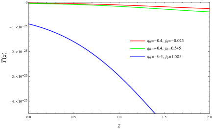
Figure 2: We display the redshift evolution of the tension of the brane $T(z)=1/f(z)$ we found in (41) using the Hubble function $H=H(z)$ reconstructed from gaussian processes applied to cosmic chronometers data. We assume $H_{0}=64.9\pm 4.2~{}kms^{-1}Mpc^{-1}$, $q_{0}=-0.4$, and $j_{0}=[-0.023,0.545,1.585]$ respectively. The tension of the brane is expressed in units of $kg/m^{3}$.

For low kinetic energy $2X=g^{\mu\nu}\phi_{,\mu}\phi_{,\nu}=\dot{\phi}^{2}\approx 0$, the Lagrangian (33) is approximated by

$$\mathscr{L}_{DBI}=X-\frac{f(\phi)}{2}X^{2}+o\left(X^{3}\right)\,,$$ (42)

where the field and its kinetic energy (e.g. its time derivative) have been treated as independent quantities. This result enlightens the difference between the Dirac-Born-Infeld theory at the core of the (Modified) Berthelot formulation, and the Generalized Born-Infeld theory which instead is the framework behind the Generalized Chaplygin Gas avelino . The latter equation of state reads as $p=-\frac{A}{\rho^{\alpha}}$ with $0<\alpha\leq 1$, and its corresponding Lagrangian has been reconstructed to be

$$\mathscr{L}_{GBI}=-A^{\frac{1}{1+\alpha}}\left[1-\left(2X\right)^{\frac{1+\alpha}{2\alpha}}\right]^{\frac{\alpha}{1+\alpha}}\,,$$ (43)

which belongs to the class of Generalized-Born-Infeld theory avelino . Setting $\alpha=1$ we obtain both the original Chaplygin Gas formulation and the Born-Infeld theory, whose Lagrangian expanded for low kinetic energy provides

$$\mathscr{L}_{BI}=X+\frac{X^{2}}{2}+o\left(X^{3}\right)\,,$$ (44)

which is a particular subcase of (42). Therefore, from the reconstruction of the underlying Lagrangian we can conclude that the (Modified) Berthelot fluid, the Generalized Chaplygin Gas and the Anton-Schmidt fluid (see luongo ) all belong to the same family of the Chaplygin gas model as they extend the Born-Infeld theory although in different directions. Furthermore, combining (25) and (36) we can write the equation of state parameter and the adiabatic speed of sound of the (Modified) Berthelot fluid as functions of the scalar field kinetic energy as:

$$w=\frac{2(2AX-B)}{B-1+\sqrt{(1+B)^{2}-8AX}}\,,\qquad c_{s}^{2}=\frac{4(2AX-B)^{2}}{(B-1+\sqrt{(1+B)^{2}-8AX})^{2}}\,,$$ (45)

where we have used

$$\rho(X)=\frac{B(B+1-\sqrt{(B+1)^{2}-8AX})-4AX}{2A(2AX-B)}\,.$$ (46)

For establishing the monotonicity properties of the speed of sound, we note that $c_{s}^{2}(\rho)$ is monotonic increasing, and we can compute

$$\frac{d\rho(X)}{dX}=\frac{B\cdot Y}{(2AX-B)^{2}\sqrt{(B+1)^{2}-8AX}}\,,\qquad Y=4AX-B^{2}-1+\sqrt{(B+1)^{2}-8AX}(1-B)\,,\qquad B<0\,,$$ (47)

where, according to the numerical analysis reported in Fig. 3, $Y$ is negative. Therefore, the sound speed squared $c_{s}^{2}=c_{s}^{2}(X)$ is monotonically increasing.

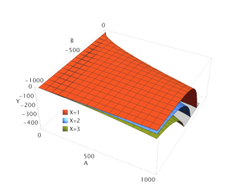
Figure 3: This figure shows the behavior of $Y=4AX-B^{2}-1+\sqrt{(B+1)^{2}-8AX}(1-B)$

over A and B for three values of $X$, namely $X=[1,2,3]$.

By inverting (38) into

$$\rho(\phi)=-\frac{1+B}{A\cosh^{2}\frac{(C-\phi)\sqrt{\frac{3(1+B)}{B}}}{2}}\,,$$ (48)

we can as well write the equation of state parameter and the adiabatic speed of sound as functions of the underlying scalar field as:

$$w=\frac{B}{1-\frac{1+B}{\cosh^{2}\frac{(C-\phi)\sqrt{\frac{3(1+B)}{B}}}{2}}}\,,\qquad c_{s}^{2}=\frac{B}{\left(1-\frac{1+B}{\cosh^{2}\frac{(C-\phi)\sqrt{\frac{3(1+B)}{B}}}{2}}\right)^{2}}\,.$$ (49)

Thus, the adiabatic speed of sound $c_{s}^{2}$ of the (Modified) Berthelot fluid is monotonic with respect to the scalar field $\phi$ in the two ranges $\phi<C$ and $\phi>C$ separately being a composition of monotonic functions there. More specifically, it is increasing in the former interval and decreasing in the latter.

III Testing the evolution of the Dieterici model at the background level

III.1 Machine Learning approach and mock datasets

When applying ML methods, we start by specifying the structure of the Neural Network, also referred to as “the model”, through a set of mathematical equations, and then we continue by running an optimisation algorithm which makes the Neural Network learn from the data it is provided with MLbook1 ; MLbook2 . In the specific Probabilistic Machine Learning, also known as Bayesian Machine Learning (BML), the learning process is repeated a large number of times for improving the ability of the Neural Network to perform its predictions, that is, to reconstruct the distribution of the posteriors. Furthermore, in this latter approach, the data are not taken from observations or experiments, but they are generated from the set of mathematical equations defining the model, that is, the model is used also for organizing the generative process which precedes the learning process MLbook1 ; MLbook2 . For fixing the ideas, in this paper we will use the model Eqs. (1)-(2) for generating the expansion rate data $H=H(z)$.

From the practical point of view, for carrying out the steps we have outlined, we exploit the probabilistic programming languages (PPLs) because they provide a complete framework for implementing BML and for computing the posterior distribution of the Neural Network parameters by applying the learning algorithm PPLs . In particular, we employ the python-based probabilistic programming package PyMC3 PyMC3 based on the deep learning library Theano which uses gradient-based Markov Chain Monte Carlo (MCMC) algorithms and Gaussian processes for generating the mock data. In our case, Eqs. (1)-(2) are employed in the generative process. Our analysis is based on $10$ chains with $3500$ generated mock datasets, where the observable is the Hubble rate as a function of the redshift $H=H(z)$.

Since these field equations can only be solved numerically, we have decided to integrate them with the help of the Runge–Kutta “RK4” method RK in which we have set the step-size $h=0.001$. The RK4 method evolves the input for the initial values, such as ($x_{n}$, $y_{n}$), into ($x_{n+1}$, $y_{n+1}$) by use of the following discretized system of equations:

$$K_{1}=h\cdot f\left(x_{n},y_{n}\right),\quad K_{2}=h\cdot f\left(x_{n}+\frac{h}{2},y_{n}+\frac{K_{1}}{2}\right),\quad K_{3}=h\cdot f\left(x_{n}+\frac{h}{2},y_{n}+\frac{K_{2}}{2}\right),\quad$$

$$K_{4}=h\cdot f\left(x_{n}+h,y_{n}+K_{3}\right),\quad y_{n+1}=y_{n}+\frac{K_{1}}{6}+\frac{K_{2}}{3}+\frac{K_{3}}{3}+\frac{K_{4}}{6}\,,$$ (50)

where $h\equiv\Delta z$, $z$ being the redshift in our case, and $f(x,y)$ is the differential equation to solve, i.e. the Friedman equations (1). Providing this algorithm with a set of initial conditions we can obtain the values of the cosmological parameters, such as the Hubble function and the matter abundance, at a certain redshift.

In the next section, we will apply BML to simulate the data $H=H(z)$ that will be used in the learning process and forecast the parameters of our cosmological model without the need for astrophysical data because the BML algorithm is able to create a mock dataset by learning from the model itself (generative process). Then, cosmic chronometers and BAO data are used to validate our results. We will carry out the generative step for the model given by Eqs. (1)-(2) over two different redshift ranges:

• $z\in[0,2.5]$ because this is the range in which the observational data for the cosmic history of the Universe are available, and they can be used for validating the results from BML.

• $z\in[0,5]$ because future explorations (like the one based on gamma-ray bursts grb ) will cover this redshift range, and their observations may be used in subsequent papers to improve the validation of the BML results.

Once we are done with the mocking of the dataset and the simulation of the Hubble function $H=H(z)$, that we will need in the learning process, using Gaussian processes, we use the available observational data about the cosmic history of the Universe to validate the BML’s forecast on the Dieterici cosmological parameters. We take the observational data from (zhang2016, , Table I). The values of the Hubble rate at different redshift reported in this dataset have been estimated by implementing the ages of passively evolving galaxies located at different redshift into the relation:

$$H(z)=-\frac{1}{(1+z)}\frac{dz}{dt}\approx-\frac{1}{(1+z)}\frac{\Delta z}{\Delta t}\,.$$ (51)

We can note that this method does not require any pre-determined assumption about the properties of the cosmic fluid and that, unlike the measurements of the luminosity distance of supernovae sources, it is based on a differential (and not integral) procedure which preserves the information about the redshift evolution of the effective EoS parameter jimenez .

III.2 Forecasts for the cosmological parameters

In this section, we exhibit the forecast bounds on the cosmological parameters entering the Dieterici model obtained applying the procedure described in Sect. III.1. We have used the package PymC3 for the generative process (which is based on Eqs. (1)-(2)) imposing flat priors on the free cosmological parameters. We summarize our forecast for the cosmological parameters in Table 1. It can be appreciated that BML imposes very tight constraints on the present-day value of dark matter abundance $\Omega_{dm0}$, on the free parameters of the Dieterici EoS, and on the Hubble constant $H_{0}$. Our results about the latter quantity suggest that a unified dark matter - dark energy paradigm pictured according to the Dieterici equation of state, in which the pressure decays exponentially with respect to the energy density, may mitigate the Hubble tension because values $H_{0}\in(70,\,72)$ km s^-1 Mpc^-1 are consistent with WMAP and South Pole Telescope estimates based on Cosmic Microwave Background datasets (eleonora, , p.11). Then, we exhibit in Fig. 4 (left panel) the contour plots of various combinations of the cosmological parameters when the data have been generated in the interval $z\in[0,2.5]$. BML imposes tight constraints on the cosmological parameters when we generate the data in the redshift range $z\in[0,5]$ as well. In this latter case, we obtain a smaller central value for $\Omega_{dm0}$. In Fig. 4 (right panel), we present the contour plots of various combinations of cosmological quantities for the analysis in this latter redshift range. Also in this case, we have assumed flat priors for the cosmological parameters.

$z$	$\Omega_{dm0}$	$H_{0}$	$A$	$B$
$z\in[0,2.5]$	$0.262\pm 0.002$	$70.992^{+0.278}_{-0.264}$ km/s/Mpc	$-2.135\pm 0.048$	$-4.506\times 10^{-5}\pm 0.314\times 10^{-5}$
$z\in[0,5]$	$0.234\pm 0.001$	$72.261^{+0.154}_{-0.146}$ km/s/Mpc	$-2.148\pm 0.019$	$-4.317\times 10^{-5}\pm 0.235\times 10^{-5}$

Table 1: The best fit values for the cosmological model given in Eqs. (1)-(2) with the corresponding $1\sigma$ errors when BML has generated the data in the two different intervals $z\in[0,2.5]$ and $z\in[0,5]$, respectively. We have searched the best fit values in the ranges $\Omega_{dm0}\in[0.2,0.5]$, $H_{0}\in[62.0,85.0]$ $km/s/Mpc$, $A\in[-5.0,0.0]$ and $B\in[-0.5,0.5]$ imposing flat priors to the cosmological parameters.

$\begin{array}[]{cccc}\includegraphics[width=256.0748pt]{Fit_NIM1.pdf}\includegraphics[width=256.0748pt]{Fit_NIM1_long.pdf}\end{array}$

Figure 4: Forecasts on the Dieterici cosmological model given by Eqs. (1)-(2) using mock data obtained from the generative process applied to these two equations. The left plot shows the results when we consider the cosmic evolution for $z\in[0,2.5]$, while in the right plot we have extended it to $z\in[0,5]$. The black contour lines show the $1\sigma$, $2\sigma$ and $2\sigma$ confidence regions, respectively.

In order to validate the outcome of our analysis, we compare in Fig.  5 the redshift evolution of the Hubble function from BML with the available combined observational data of cosmic chronometers and BAO. In the plot, the purple curve refers to the case in which we have generated the data for $z\in[0,2.5]$, while the dashed red curve holds when $z\in[0,5]$. The dots are the 40 data points from astrophysical observations taken from (zhang2016, , Table I). We can note that the BML result for the redshift evolution of the Hubble function is in good agreement with the observational data at low redshift, but some tension could arise at high redshift. Indeed, the two estimates of $H_{0}$ reported in Table 1 are not consistent with each other at 1$\sigma$ level.

In Fig. 6, we display the redshift evolution of the deceleration parameter $q$ (left panel) and of the effective EoS parameter of the Dieterici fluid $w$ (right panel), for the best fit values of the model parameters exhibited in Table 1. We use the same convention for the purple and dashed red curves as in Fig. 5. We can see that the BML analysis predicts a transition between a decelerating and an accelerating phase of the Universe. More quantitatively, we obtain that the transition to a negative deceleration parameter, e.g. to the present epoch of accelerated expansion of the Universe, occurs at a lower value of the redshift, e.g. more recently, when our analysis relies on the data in $z\in[0,\,2.5]$. In other words, the Dieterici model exhibits a correlation between a more recent transition and a lower value of the Hubble constant $H_{0}$ and an higher value of the present day dark matter abundance $\Omega_{dm0}$. Furthermore, from the plot in the right panel, one can understand that the Dieterici fluid behaves as a phantom fluid at the present epoch because $w<-1$.

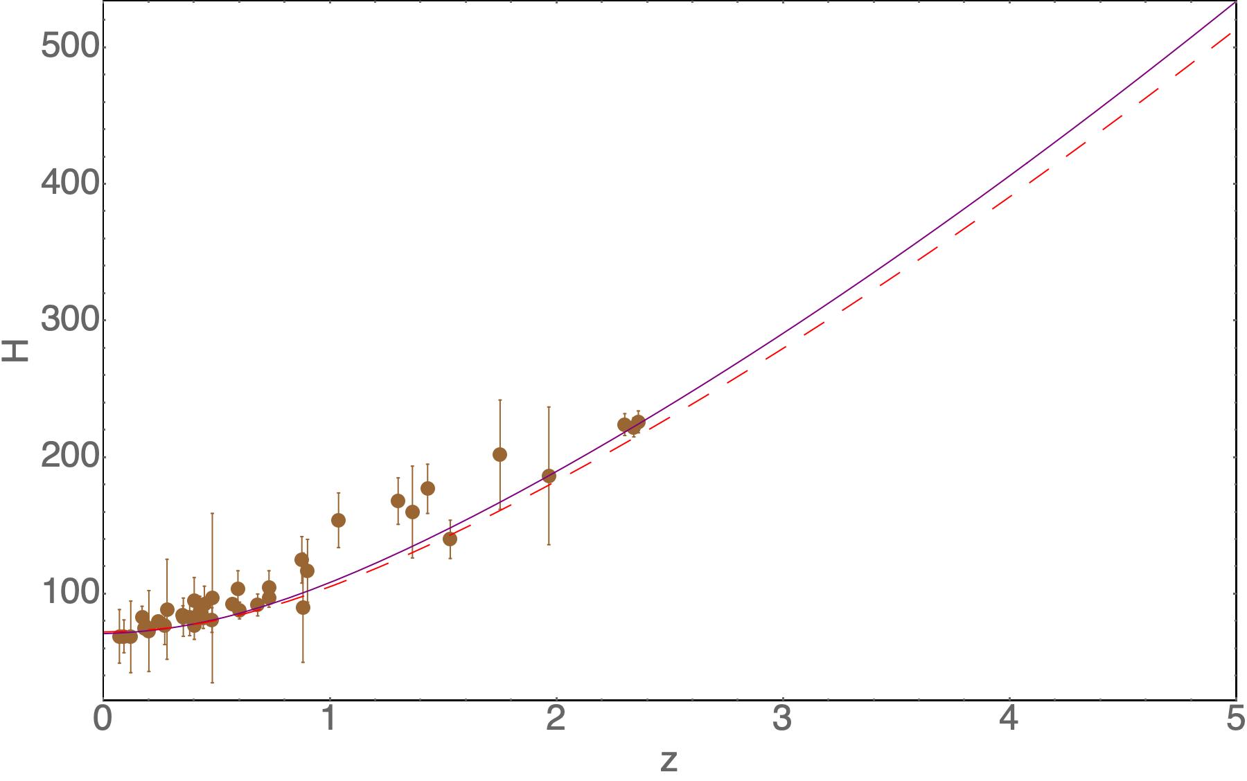
Figure 5: The BML prediction for the redshift evolution of the Hubble function $H=H(z)$ compared to the cosmic chronometers and BAO data (red dots) from (zhang2016, , Table I). The purple curve has been obtained when the data are generated in $z\in[0,2.5]$, while the dashed red curve takes into account the data generated in $z\in[0,5]$. The free parameters affecting the two curves have been fixed as reported in Table 1.

$\begin{array}[]{cccc}\includegraphics[width=213.39566pt]{q_Model_1.jpeg}&&\includegraphics[width=213.39566pt]{w_Model_1.jpeg}\\ \end{array}$

Figure 6: BML predictions for the redshift evolution of the EoS parameter $w$ (right panel) and deceleration parameter $q$ (left panel). The same conventions on the types of the curves as in Fig. 5 apply.

IV On some cosmic model degeneracy, and its breaking

IV.1 Cosmic opacity and model degeneracy

The dark energy abundance can be estimated by analyzing the luminosity distance data of type Ia supernovae; historically, this was the first astrophysical observation that had called for the introduction of such a mysterious fluid. Therefore, ultimately it is necessary to reconstruct the flux of photons arriving from those sources: light rays travel along geodesics experiencing the spacetime curvature, which is assumed constant in the usual Friedman-Lemaître-Robertson-Walker model. It has been claimed that non-constant curvature effects along the photons’ path may mimic some observational properties attributed to dark energy inhom1 ; inhom2 ; inhom3 ; inhom4 ; inhom5 ; inhom6 ; inhom7 . On the other hand, scattering and absorption effects with the interstellar medium can affect the propagation of light rays as well. This means that photons do not travel through a perfectly transparent region whose opacity should be considered as a redshift dependent function $\eta=\eta(z)$. According to this framework, the dark energy abundance $\Omega$ and its equation of state parameter $w(z)$ should be found by comparing astrophysical data against the corrected luminosity distance function, which, for for a flat universe, reads

$$D_{L}=(1+z)\eta(z)\int_{0}^{z}\frac{dz^{\prime}}{\sqrt{(1-\Omega)(1+z^{\prime})^{3}+\Omega{\rm Exp}\left[3\int_{0}^{z^{\prime}}\frac{1+w(\bar{z})]d\bar{z}}{1+\bar{z}}\right]}}\,,$$ (52)

where the idealized case of a perfectly transparent universe is recovered for $\eta(z)\equiv 1$. A plethora of different possibilities for the opacity function $\eta(z)$ has been proposed in the literature for implementing information about many different phenomena which may affect the travel of photons as scattering, absorption, and gravitational lensing effects experienced by the light rays when travelling inside some dust clouds or nearby massive astrophysical objects. For example, in Lee the applicability of some proposals of the cosmic opacity as $\tau(z)=2\epsilon z$, $\tau(z)=(1+z)^{2\epsilon}-1$, $\eta(z)=\eta_{0}$, $\eta(z)=\eta_{0}+\eta_{1}z$, $\eta(z)=\eta_{0}+\eta_{1}z/(1+z)$, $\eta(z)=\eta_{0}+\eta_{1}z/(1+z)^{2}$, $\eta(z)=\eta_{0}-\eta_{1}\ln(1+z)$, $\eta(z)=\eta_{0}/(1+z)$, $\eta(z)=\eta_{0}/(1+z)\exp[z/(1+z)]$, $(1+z)^{\eta_{0}}$, where $\epsilon$, $\eta_{0}$ and $\eta_{1}$ are free model parameters, have been tested in light of relevant astrophysical datasets as Union2, SDSS, 6dFGS, WiggleZ, BOSS, BAO, etc… . Already in the past decade there were investigations on the redshift evolution of the cosmic opacity eta1 ; eta2 ; eta3 ; eta4 similarly to what done for the dark energy equation of state parameter w1 ; w2 ; w3 ; w4 ; recently these studies have acquired a novel relevance in light of the Hubble tension issue PyMC3_p2 .

However, the following problem arises: it is conceivable that completely different pairs ($\tau(z)$, $w(z)$) will perform statistically equivalently with the cosmic opacity function somehow masking the properties of the dark energy fluid. Let us explain what we mean by considering the following simple example of known analytical luminosity distances; modulo some technicalities, the same reasoning can be extended to the dark energy fluid models. The luminosity distances in the Milne and Einstein-De Sitter universes are respectively given by Hogg

$$d_{L1}(z)=z\left(1+\frac{z}{2}\right)\,,\qquad d_{L2}(z)=2(1+z-\sqrt{1+z})\,.$$ (53)

By multiplying $d_{L2}(z)$ by the cosmic opacity function

$$\eta_{A}(z)=\frac{z(2+z)}{4(1+z-\sqrt{1+z})}$$ (54)

we will get the luminosity distance $d_{L1}(z)$. Next, we should note that $\eta_{A}(z)$ can be well-approximated by some cosmic opacity functions which had already arisen in previous literature suggesting that it is not a completely ad-hoc result. See Fig. 7, in which we compare graphically $\eta_{A}(z)$, with $\eta_{B}=\eta_{0}+\eta_{1}z/(1+z)$, $\eta_{C}=\eta_{0}-\eta_{1}\ln(1+z)$ with $[\eta_{0}\approx 0.90,\,\eta_{1}\approx 0.88]$ and $[\eta_{0}\approx 0.98,\,\eta_{1}\approx-0.46]$ respectively, $\eta_{D}=\eta_{0}+\eta_{1}z$ with $[\eta_{0}\approx 0.98,\,\eta_{1}\approx 0.30]$, and $\eta_{E}=(1+z)^{\eta_{0}}$ with $\eta_{0}\approx 0.41$.

Therefore, we must find some specific signatures for breaking the degeneracy between cosmological models based on different pairs cosmic opacity - dark energy equation of state. In the next section, we will tackle this problem by applying perturbation techniques because they are sensitive to the dark energy equation of state only. Consequently, our reasoning is analogue to what explored in Chakraborty in which the degeneracy at a background level between $\Lambda$CDM and a specific $f(R)$ modified gravity model was broken by tracking the evolution of the density perturbations; this way of thinking has already helped also in differentiating between dark interactions differentiating . Likewise, it has been possible as well to discriminate between some $f(T)$ gravitational theories and their background equivalent dark energy fluid models by looking at growth of perturbations referee .

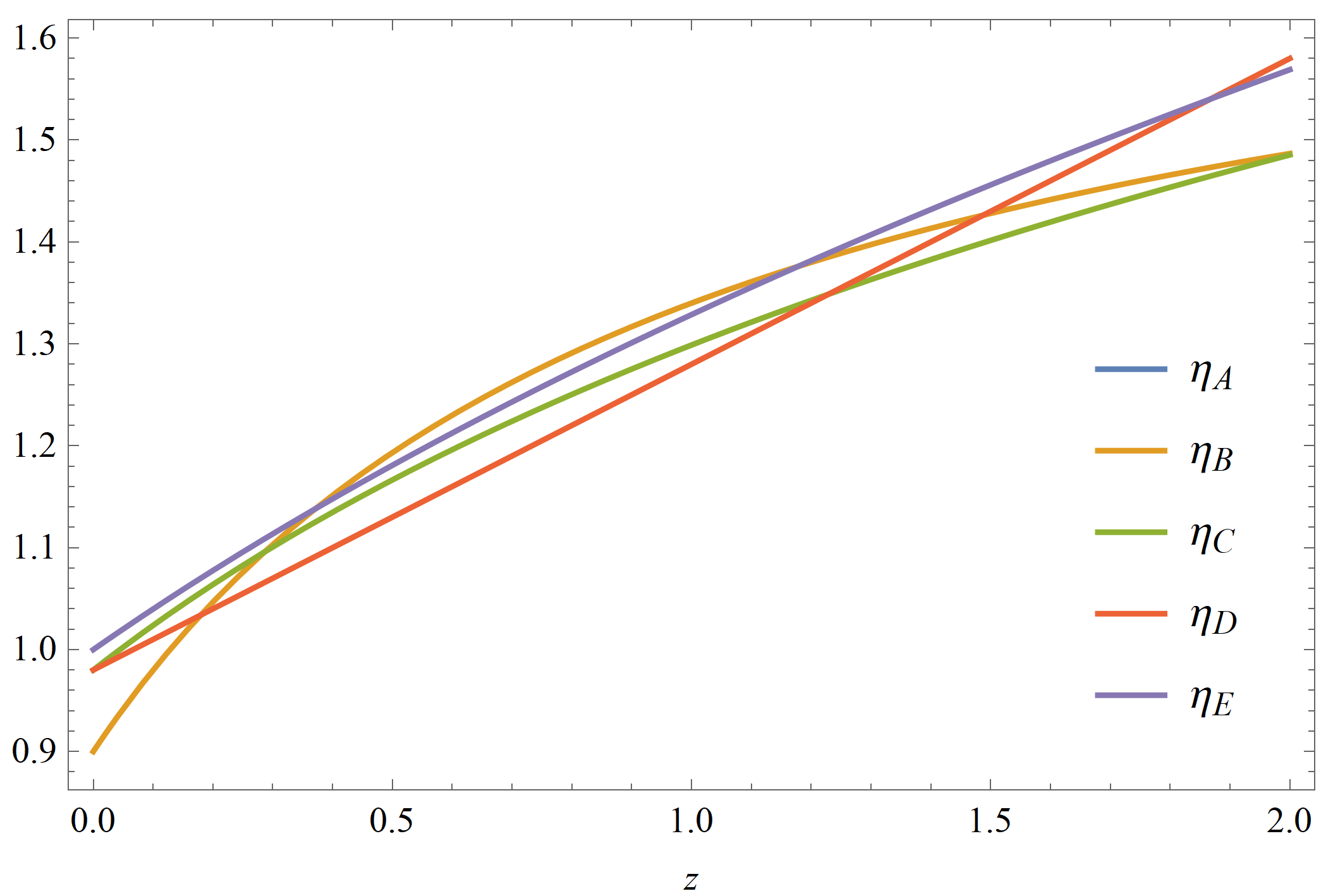
Figure 7: The cosmic opacity function $\eta_{A}(z)$ (54), which would lead to a degeneracy between the luminosity distances of the Milne and Einstein-De Sitter universes, is compared with some other cosmic opacity functions proposed in other literature, namely $\eta_{B}=\eta_{0}+\eta_{1}z/(1+z)$, $\eta_{C}=\eta_{0}-\eta_{1}\ln(1+z)$ with $[\eta_{0}\approx 0.90,\,\eta_{1}\approx 0.88]$ and $[\eta_{0}\approx 0.98,\,\eta_{1}\approx-0.46]$ respectively, $\eta_{D}=\eta_{0}+\eta_{1}z$ with $[\eta_{0}\approx 0.98,\,\eta_{1}\approx 0.30]$, and $\eta_{E}=(1+z)^{\eta_{0}}$ with $\eta_{0}\approx 0.41$. Qualitative similarities are noteworthy.

IV.2 Breaking the model degeneracy through perturbation analysis

The equation governing the evolution of the density perturbation is given by (WE, , Chapert 14)

$$\ddot{\delta}+A(t)H\dot{\delta}+\left(B(t)+\frac{c_{s}^{2}n^{2}}{H^{2}a^{2}}\right)H^{2}\delta=0,$$ (55)

where $\delta$ is the density fluctuation, $n$ is the wave-number of the Fourier mode of the perturbation, and

$$A(t)=2-3\omega-3\left(\omega-c_{s}^{2}\right)\,,\qquad B(t)=-\frac{3}{2}\left[(1-\omega)(1+3\omega)+6\left(\omega-c_{s}^{2}\right)\right]\Omega+\frac{12k}{H^{2}a^{2}}\left(\omega-c_{s}^{2}\right)\,,$$ (56)

where $\omega=p/\rho$, $c_{s}^{2}=\frac{\partial p}{\partial\rho}$ and $k$ is the spatial curvature of the Friedman universe.

Perturbation analysis for a universe filled by the Chaplygin gas has revealed that a phase of growing perturbations occurs at early times, which is followed by a decreasing oscillatory phase at late times asymptotically going to zero P.chap . On the other hand, for Logotropic and Anton-Schmidt fluids, considering the best-fit parameters with respect to Pantheon supernovae data, observational Hubble data, and $\sigma_{8}$ data points, it has been pointed out in anton that matter perturbations decrease in time and remain bound, except for the model in which the Grüneisen parameter is fixed at priori in which case the perturbations are diverging at early times. For these latter models, there is no oscillatory behavior.

If we consider a flat single-fluid universe (for which $\Omega=1$) and introduce the energy contrast defined as $\xi=\delta(t)/\rho(t)$, by expanding the time derivatives and eliminating the ones of the energy density via $\dot{\rho}=-\sqrt{3\rho(t)}(\rho(t)+p(t))$, we can express (55) in the long-wavelength limit (i.e. $n/(Ha)\ll 1$) as

$$\ddot{\xi}+\sqrt{\frac{\rho(t)}{3}}(3c_{s}^{2}-12\omega-4)\dot{\xi}+\left(3c_{s}^{2}+9\omega^{2}+6\omega+2\right)\rho(t)\xi=0\,,$$ (57)

where we have eliminated the Hubble function by using the Friedman equation $H(t)=\sqrt{\rho(t)/3}$. We will now discuss in some detail the evolution of the density contrast in universes filled by the (Modified) Berthelot and the Dieterici fluids separately focusing on their weakly nonlinear regimes for which analytical solutions in terms of special functions can be found. We will as well focus on the effects beyond the background level.

Beginning with the (Modified) Berthelot fluid, we approximate the solution to its background energy conservation equation as $\rho(t)\sim\frac{4}{3t^{2}(B+1)^{2}}$. Implementing it into (57) and keeping only the leading order terms in $A$ we obtain

$$A(t)\ddot{\xi}+B(t)\dot{\xi}+C(t)\xi=0\,,\qquad A(t)=\frac{t^{2}(B+1)^{2}\left(8A+3(B+1)^{2}t^{2}\right)}{3}\,,$$ (58)

$$B(t)=-\frac{2t(B+1)[3(1+B)^{2}(9B+4)t^{2}+16A(3B+2)]}{9}\,,\qquad C(t)=\frac{4(3B+2)\left(8A+3(3B+1)(B+1)^{2}t^{2}\right)}{9}.$$ (59)

This equation can be solved analytically as

$$\xi(t)=C_{1}t^{\frac{15B+11+\beta}{6\left(B+1\right)}}\cdot h_{1}(t)+C_{2}t^{\frac{15B+11-\beta}{6\left(B+1\right)}}\cdot h_{2}(t)$$ (60)

where $C_{1}$ and $C_{2}$ are constants of integration, $\beta=\sqrt{225B^{2}+186B+25}$, and $h_{1}$ and $h_{2}$ are the following hypergeometric functions:

$$h_{1}(t) = {}_{2}F_{1}\left(\left[\frac{\beta-9B-5}{12(B+1)},\,\frac{5+\beta-3B}{12(B+1)}\right],\,\left[\frac{6(B+1)+\beta}{6(B+1)}\right];\,-\frac{3\left(B+1\right)^{2}t^{2}}{8A}\right)\,,$$ (61)

$$h_{2}(t) = {}_{2}F_{1}\left(\left[\frac{5-3B-\beta}{12(B+1)},\,-\frac{5+3B+9\beta}{12(B+1)}\right],\,\left[\frac{(6B+1)-\beta}{6(B+1)}\right];\,-\frac{3\left(B+1\right)^{2}t^{2}}{8A}\right)\,.$$ (62)

For an intuitive visual representation of the evolution of the density contrast in a universe filled with a (Modified) Berthelot fluid with small non-linearities, we integrate backwards in time (58)-(59) with initial conditions $\xi(1.10)=0.01$, $\dot{\xi}(1.10)=0.01$, and with $A=0.1$ and various choices for $B$; the result is presented in Fig. 8 (panel a). We obtain that for all values of the parameter $B$ we have investigated, the density contrast $\xi$ is monotonically decreasing in time in the interval considered.

For the case of a universe filled with a Dieterici fluid, inserting again the approximated result for the energy conservation law at the background level $\rho(t)\sim\frac{4}{3t^{2}(A+1)^{2}}$ into (57), and approximating $B\approx 0$, we arrive at an equation for the evolution of density contrast analogous to (58) but with the following time-dependent coefficients:

$$A(t)=9t^{6}(1+A)^{6}\,,\qquad B(t)=-2(A+1)t\left(8AB^{2}+3(9A+4)(A+1)^{4}t^{4}+24A(A+1)^{2}Bt^{2}\right)\,,$$ (63)

$$C(t)=4\left(8A(12A+5)B^{2}+3(1+3A)(2+3A)(A+1)^{4}t^{4}+24A(3A+2)(A+1)^{2}Bt^{2}\right)\,.$$

In this case, the general solution for the evolution of the density contrast is:

$$\xi(t)=\left[C_{3}t^{\frac{12A+8}{3(A+1)}}\cdot{\rm HeunB}\left(-a,b,c,d;\frac{2\sqrt{A}B}{3(A+1)^{5/2}t^{2}}\right)+C_{4}t^{\frac{3A+1}{A+1}}\cdot{\rm HeunB}\left(a,b,c,d;\frac{2\sqrt{A}B}{3(A+1)^{5/2}t^{2}}\right)\right]\cdot{\rm Exp}\left(-\frac{4\left[6t^{2}(A+1)^{2}+B\right]AB}{9(A+1)^{5}t^{4}}\right)\,,$$

$$a=\frac{3A+5}{6(A+1)},\qquad b=4\sqrt{\frac{A}{A+1}},\qquad c=\frac{37(3A+1)}{6(A+1)},\qquad d=-\frac{2\left(9A+7\right)\sqrt{A}}{3(A+1)^{3/2}}\,,$$ (64)

where $C_{3}$ and $C_{4}$ are constants of integration and HeunB denotes the Heun’s Biconfluent special function. For an intuitive visualization, we display the evolution of the density contrast in a universe filled with a Dieterici fluid with initial conditions $\xi(1.10)=0.01$, $\dot{\xi}(1.10)=0.01$, setting $B=-0.1$ and assuming various values of $A$ in Fig. 8 (panel b). We obtain that the density contrast $\xi$ exhibits an increasing and oscillatory behavior in time for the values of $A$ and the time interval we have considered. We can therefore appreciate important qualitative differences between panels (a) and (b), e.g. between the evolution of the density contrast for the (Modified) Berthelot and Dieterici fluids. The instabilities identified in the latter scenario might be related to the corresponding evolution of the speed of sound, which governs their velocity of propagation, and which contains an exponential factor $\sim e^{\rho}\sim e^{1/t^{2}}$. This factor amplifies the (negative) value of the adiabatic speed of sound in the time interval we have considered, and can actually serve as an hint for identifying this suitable time interval necessary for breaking the degeneracy.

$\begin{array}[]{cccc}\includegraphics[width=241.84842pt]{xiMo.pdf}&&\includegraphics[width=241.84842pt]{xiD.pdf}\\ (a)&&(b)\end{array}$

Figure 8: The time evolution of the density contrast $\xi=\delta/\rho$ for a single fluid flat universe filled with (Modified) Berthelot fluid (panel a) and Dieterici fluid (panel b) for four values of B=[-2.0,-1.7,-1.5,-1.3] and A=[-2.0,-1.7,-1.5,-1.3], respectively for the two models. In panel (a), we have integrated backwards in time eqs. (58)-(59) with initial conditions $\xi(1.10)=0.01$, $\dot{\xi}(1.10)=0.01$ and fixing $A=0.1$. In panel (b), we have integrated backwards in time eqs.(58)-(63) with the same initial conditions as panel (a) but fixing $B=-0.1$.

V $k$-essence and free Dirac-Born-Infeld as dark matter candidates only

In this section, we will assess whether the two fluid models we have previously introduced, namely the Dieterici and (Modified) Berthelot equations of state, can account or not for flat galactic rotation curves. We are here assuming that these models can be adopted for a description of the dark matter content of the universe, and this section should be considered as in parallel to the ones in which those models have instead been invoked as candidates for the dark energy budget. Indeed, there has been a recent interest in quantifying the effects of a non-zero adiabatic speed of sound of dark matter, as arising in our models, on galactic scales malafarina . In particular, we will show that the free Dirac-Born-Infeld model cannot account for flat rotation curves and a specific condition on the potential for achieving this goal is proposed. The gravitational potential withing the galaxy will also be written in a closed form with respect to the energy density allowing us to discuss a possible physical reason on the different applicability of the two models.

V.1 Galaxies Rotation Curve in the Dieterici and (Modified) Berthelot frameworks

Following (malafarina, , Eqs.(5)-(6)-(7)), we describe the dark matter density profile far away from the center of the galaxy adopting the newtonian equations of hydrodynamic equilibrium, which read as:

$$\frac{dM(r)}{dr} = 4\pi r^{2}\rho(r)\,,$$ (65)

$$\frac{dP(r)}{dr} = -\rho(r)\frac{M(r)}{r^{2}}\,,$$ (66)

$$\frac{d\Phi(r)}{dr} = \frac{M(r)}{r^{2}}\,,$$ (67)

where $M(r)$ is the mass of the galaxy contained in a sphere of radius $r$, and $\Phi(r)$ is the gravitationl potential. Then, it can be shown that the rotation velocity is malafarina

$$v=\sqrt{\frac{M(r)}{r}}\,.$$ (68)

Eq.(66) can be rewritten as

$$c_{s}^{2}\frac{d\rho(r)}{dr}=-\rho(r)\frac{M(r)}{r^{2}}\,,$$ (69)

which has been used for assessing the effects of a non-zero speed of sound of dark matter in the galactic rotation curves malafarina ; kuantay , and which for the case of the Dieterici fluid becomes explicitly

$$\frac{d\rho(r)}{dr}=-\frac{\rho(r)\,M(r)\,e^{-B\rho(r)}}{Ar^{2}(1+B\rho(r))}\,.$$ (70)

Differentiating both sides of (65) with respect to $r$, plugging in (70), and finally eliminating the energy density via $\rho(r)=\frac{dM(r)}{4\pi r^{2}dr}$ we obtain the differential equation

$$4\frac{dM(r)}{dr}{\rm Exp}\left[-\frac{B\,dM(r)}{4\pi r^{2}dr}\right]\pi rM(r)+A\left(r\frac{d^{2}M(r)}{dr^{2}}-2\frac{dM(r)}{dr}\right)\left(4\pi r^{2}+B\frac{dM(r)}{dr}\right)=0\,,$$ (71)

which governs the radial behavior of the mass of the galaxy. Next, we assume a power-law profile with $M(r)\sim r^{\alpha}$ into the previous condition arriving at

$$4\pi r^{\alpha}{\rm Exp}\left[-\frac{B\alpha r^{\alpha-3}}{4\pi}\right]+A(\alpha-3)(B\alpha r^{\alpha-2}+4\pi r)=0\,.$$ (72)

For obtaining a flat rotation curve at spatial infinity by using (68), we need to require $\alpha=1$, with the previous condition now reading

$$4\pi re^{-\frac{B}{4\pi r^{2}}}-2A\left(\frac{B}{r}+4\pi r\right)=0\,,$$ (73)

whose asymptotic behavior is

$$4\pi(1-2A)r+O\left(\frac{1}{r}\right)=0\,,$$ (74)

showing that a Dieterici fluid model can account for asymptotically flat galactic rotation curves with (in natural units) $A=1/2$.

On the other hand, the explicit realization of (66) for a (Modified) Berthelot fluid is

$$\frac{d\rho(r)}{dr}=-\frac{\rho(r)M(r)(1+A\rho(r))^{2}}{r^{2}B}\,,$$ (75)

and Eq.(71) should now be replaced by

$$16Br^{6}\pi^{2}\frac{d^{2}M(r)}{dr^{2}}+16\pi^{2}r^{4}\left(M(r)-2Br\right)\frac{dM(r)}{dr}+8A\pi r^{2}M(r)\left(\frac{dM(r)}{dr}\right)^{2}+A^{2}M(r)\left(\frac{dM(r)}{dr}\right)^{3}\,.$$ (76)

Assuming again a power-law profile $M(r)\sim r^{\alpha}$ with $\alpha=1$, we obtain

$$32\left(\frac{1}{2}-B\right)\pi^{2}r^{4}+8A\pi r^{2}+A^{2}=0\,,$$ (77)

which shows that a (Modified) Berthelot fluid cannot account for flat galaxy rotation curves. Hence, $k$-essence models and free Dirac-Born-Infeld models exhibit completely different applicability as dark matter candidates.

Finally, from (67),(69) we can write a differential equation for the gravitational potential with respect to the fluid density

$$\frac{d\Phi(\rho)}{d\rho}=-\frac{c_{s}^{2}}{\rho}\,,$$ (78)

which, recalling (7), (25), can be solved as

$$\Phi(\rho) = A[{\rm Ei}(1,-B\rho)-e^{B\rho}]+{\mathscr{C}}_{1}\,,$$ (79)

$$\Phi(\rho) = B\left[\ln\frac{1+A\rho}{\rho}-\frac{1}{1+A\rho}\right]+{\mathscr{C}}_{2}\,,$$ (80)

for the Dieterici and the (Modified) Berthelot fluids respectively, where ${\mathscr{C}}_{1}$ and ${\mathscr{C}}_{2}$ are some constants of integration. We further notice that

$$\frac{d\Phi}{dc_{s}^{2}} \equiv \frac{d\Phi(\rho)}{d\rho}\cdot\frac{1}{\frac{dc_{s}^{2}}{d\rho}}\,=\,-\frac{B\rho+1}{B\rho(2+B\rho)}\,,$$ (81)

$$\frac{d\Phi}{dc_{s}^{2}} \equiv \frac{d\Phi(\rho)}{d\rho}\cdot\frac{1}{\frac{dc_{s}^{2}}{d\rho}}\,=\,\frac{1+A\rho}{2A\rho}>0\,,$$ (82)

for the two equations of state respectively. While in the latter case $\Phi=\Phi(c_{s}^{2})$ is an increasing monotonic function, this is not in the former case: this can constitute the physical reason behind the different clustering properties of the two fluids. As an interesting result, recalling (27), we can also relate the Newtonian potential within the galaxy to the Lagrangian scalar field potential in the non-relativistic regime for the (Modified) Berthelot fluid:

$$\Phi(r)=-\frac{dV}{d\rho}\,.$$ (83)

V.2 Galaxies Rotation Curves in the DBI framework

Exploiting that the (Modified) Berthelot fluid is the hydrodynamical realization of the free Dirac-Born-Infeld model, we could claim that the latter is challenged by astrophysical requirements of flat galactic rotation curves. Therefore, we would like now to investigate whether these observations can be used for reconstructing some information on the potential of the scalar field. Requiring an almost vanishing pressure $p=0$ in (34), we obtain the condition

$$V(\phi)=\frac{2\gamma X}{1+\gamma}\,,$$ (84)

or in other words

$$X=V(\phi)\left(1-\frac{V(\phi)f(\phi)}{2}\right)\,.$$ (85)

This requirement sets a constraint between the kinetic energy $X$ and the scalar field itself $\phi$, and therefore for the cosmic energy density $\rho(X,\phi)\,\,\to\,\,\rho(\phi)$. We interpret this result as imposing a relationship such that in the dark matter dominated era the time evolution of the potential is such that $V(t)=\frac{2\gamma X(t)}{1+\gamma}$; see for example (bertacca, , Eq.(20)) and the $f=f(\phi(X))$ formalism which follows from imposing a certain condition on the pressure. Explicitly we obtain

$$\rho(\phi)=\frac{[2-f(\phi)V(\phi)]V(\phi)}{1-f(\phi)V(\phi)}\,.$$ (86)

The adiabatic speed of sound in (34), once (85) is implemented, reads as

$$c_{s}^{2}=1-f(\phi)V(\phi)\,.$$ (87)

We note that

$$\dot{X}=\dot{\phi}\ddot{\phi}\qquad\Rightarrow\qquad\ddot{\phi}=\frac{\dot{X}}{\dot{\phi}}=\frac{\frac{dX}{d\phi}\cdot\dot{\phi}}{\dot{\phi}}=\frac{dX}{d\phi}\,,$$ (88)

where the relationship (85) is understood. Requiring a dark-matter-like behavior also for the speed of sound (87), e.g. $c_{s}^{2}\approx 0$, we further write $V(\phi)=\frac{b}{f(\phi)}$ with $b$ some constant whose value in natural units is close to 1. Therefore, we obtain

$$c_{s}\approx\sqrt{1-b}\,,\qquad H=\sqrt{\frac{\rho(\phi)}{3}}\approx\sqrt{\frac{(2-b)b}{3(1-b)f(\phi)}}\,,\qquad\frac{dX}{d\phi}\approx\frac{f^{\prime}(\phi)}{f^{2}(\phi)}\left(\frac{b}{2}-1\right)\,.$$ (89)

Under our assumptions, the equation of motion of a Dirac-Born-Infeld scalar field (see e.g. DBI_inf1 )

$$\ddot{\phi}+3Hc_{s}^{2}\dot{\phi}+c_{s}^{3}V^{\prime}(\phi)+\frac{f^{\prime}(\phi)}{2f(\phi)}\left(1-\frac{2c_{s}^{2}}{1+c_{s}}\right)\dot{\phi}^{2}=0\,,$$ (90)

where a prime denotes a derivative with respect to $\phi$, becomes

$$\sqrt{1-b}[4b^{2}-5b-2-(2+b)\sqrt{1-b}]f^{\prime}(\phi)+2\sqrt{3}b(b-2)(1-\sqrt{1-b})f(\phi)\approx 0\,,$$ (91)

which comes with the solution

$$f(\phi)=Ce^{-D\phi}\,,\qquad D\equiv\frac{2\sqrt{3}b(b-2)(1-\sqrt{1-b})}{\sqrt{1-b}[4b^{2}-5b-2-(2+b)\sqrt{1-b}]}\,,$$ (92)

where $C$ is an arbitrary constant of integration. The equation for hydrostatic equilibrium can be rewritten in terms of the scalar field, rather than of the energy density, as

$$\frac{d\phi}{dr}=\frac{1}{\frac{d\rho}{d\phi}}\cdot\frac{d\rho}{dr}\approx\frac{f(\phi)M(r)}{(1-b)f^{\prime}(\phi)r^{2}}=\frac{M(r)}{(b-1)Dr^{2}}\,.$$ (93)

Taking a derivative with respect to the radial coordinate $r$ and using (65) with $\rho\approx\frac{(2-b)b}{(1-b)f(\phi(r))}$ we obtain the second order differential equation governing the radial behavior of the scalar field:

$$\frac{d^{2}\phi}{dr^{2}}+\frac{2}{r}\frac{d\phi}{dr}+\frac{4\pi b(2-b)}{(1-b)^{2}D\,C}e^{D\phi}=0\,.$$ (94)

By introducing the auxiliary variable $\phi(r)=\ln Y(r)$, the condition for hydrostatic equilibrium for the scalar field becomes

$$Y(r)\frac{d^{2}Y(r)}{dr^{2}}-\left(\frac{dY(r)}{dr}\right)^{2}+\frac{2Y(r)}{r}\frac{dY(r)}{dr}+\frac{4\pi b(2-b)}{(1-b)^{2}D\,C}Y^{D+2}(r)=0\,.$$ (95)

Substituting a power-law solution $Y(r)\sim r^{j}$ we get $j+\frac{4\pi b(2-b)}{(1-b)^{2}D\,C}r^{Dj+2}\sim 0$ which, by dimensional analysis, delivers $j=-2/D$, and therefore $\phi(r)\sim\ln r^{-2/D}$. Then, recalling (92), which provides $f(\phi(r))\sim Cr^{2}$, and (86) we obtain the radial profile of the energy density as

$$\rho(r)\sim\frac{(2-b)b}{(1-b)Cr^{2}}\,.$$ (96)

It can be appreciated that among the various possible dark matter profile, e.g. the ISO profile, exponential sphere, Burkert profile, NFW profile, Moore profile, Einasto profile, ours is well approximated at large distances from the center by the former ISOprofile :

$$\rho_{\rm ISO}(r)=\frac{\rho_{0}}{1+\left(\frac{r}{r_{0}}\right)^{2}}\,\to\,\frac{\rho_{0}r_{0}}{r^{2}}\,,\qquad\rho_{0}r_{0}=\frac{(2-b)b}{(1-b)C}\,.$$ (97)

Then, from (65) and (68) we get the rotation velocity of the galactic curve to be

$$v\approx\sqrt{\frac{4\pi(2-b)b}{(1-b)C}}\,.$$ (98)

Deepening the exploration of our Dirac-Born-Infeld model as dark matter candidate only, we discuss here the formation of cosmic structures, and then use this result jointly with the previous analysis for estimating the dark matter speed of sound within the galaxy. We begin by writing the comoving Jeans length in the matter dominated era as (logofereira, , Sect.IV)

$$\lambda^{c}_{J}=c_{s}(1+z)\left(\frac{\pi}{\rho}\right)^{1/2}\,.$$ (99)

In the matter-dominated era, in which $p\approx 0$ and $c_{s}^{2}\approx 0$ hold, we have $\rho(X)\approx\frac{2X}{1-b}=\frac{\dot{\phi}^{2}}{1-b}$. Therefore, from the Friedman equation and (51) we arrive at

$$\frac{dz}{dt}=-\frac{(1+z)\dot{\phi}}{\sqrt{3(1-b)}}\,,\qquad\Rightarrow\qquad\phi(z)=-\sqrt{3(1-b)}\,\ln(1+z)\,.$$ (100)

Still using the conditions stemming from $p\approx 0$ and $c_{s}^{2}\approx 0$, and eqs.(86), (92) we get from (99)

$$\lambda^{c}_{J}\approx(1-b)\sqrt{\frac{\pi C}{(2-b)b}}(1+z_{c})^{1-\frac{D\sqrt{3(1-b)}}{2}}\,,$$ (101)

where $z_{c}\approx 1$ (logofereira, , Sect.IV). Isolating for $C$, taking into account (98), we can finally write for $b\approx 1$

$$c_{s}\approx\frac{\lambda^{c}_{J}v}{2\pi(1+z_{c})}\,.$$ (102)

Re-introducing the Hubble constant for working in International System Units, and considering now $\lambda^{c}_{J}\approx R\approx 8h^{-1}$, $h\approx 0.73$ and $v\approx 130$ km/s, we get $c_{s}\approx 113$ km/s in good agreement with the result for the adiabatic speed of sound of dark matter in the halo (malafarina, , Table III).

VI Conclusion

Although the Dirac-Born-Infeld theory has been originally proposed for taming the divergence of the electron self-energy as computed in classical electrodynamics ED1 ; ED2 , it has received novel attention in recent decades in cosmological applications. One or multiple DBI_inf2 scalar field(s), possibly non-minimally coupled to other kinetic terms DBI_inf3 , to radiation DBI_inf4 , or to perfect fluids DBI3 , arising in the DBI framework may govern the inflationary epoch in the slow-roll regime string2 . In this paper, we have proposed a Dirac-Born-Infeld interpretation for the fluid model (3) by assuming a vanishing potential: since the applicability of that fluid model was already put forward in capo , our analysis may complement that of DBI2 in which specific DBI potentials were shown to give raise to fluid models challenged by observational datasets. Our result for the relation between the adiabatic speed of sound and DBI scalar field (49) for the (Modified) Berthelot fluid may be used in future projects for further assessing this specific realization of the cosmic matter content in light of the primordial black hole mass function invoking the sound speed resonance mechanism following DBI_inf1 , or tracking the amplification of the curvature perturbations as in tronconi . Models belonging to the DBI family may also be applied for describing other thermal epochs of the universe DBI4 ; DBI5 either accounting for the dark energy abundance solely DBI6 , also specifically reproducing the cosmological constant term DBI8 , or for its unified form with dark matter DBI7 . This class of models provides various opportunities for realizing an accelerated phase of expansion of the universe DBI9 even possibly taming the coincidence problem DBI13 . Being interested in this paper in an application in late-time cosmology, we have computed the relationship between the tension of the DBI brane generating the (Modified) Berthelot fluid model and the cosmographic parameters in (41) and presented its redshift evolution in Fig. 2. The most important take-at-home messages at the core of this manuscript, which can play a role as well in future applications, are: (i) the (Modified) Berthelot fluid is the hydrodynamic realization of the free Dirac-Born-Infeld theory; (ii) the free Dirac-Born-Infeld theory cannot account for flat galactic rotation curves; (iii) an exponential potential inversely proportional to the brane tension can fix this problem at a satisfactory level as shown by the predicted value of the adiabatic speed of sound of dark matter in the halo.

Furthermore, in this paper, we have also shown that another cosmological model proposed in dieterici1 as a dark matter - dark energy unification, e.g. the Dieterici one, does not challenge the Generalized Chaplygin Gas in the description of the cosmic history of the Universe. Even though the qualitative characteristics of the two models are similar, that is, they can both interpolate between decelerating and accelerating phases of the Universe, our quantitative analysis has shown that the cosmic chronometers and BAO data do not favor the former. In fact, the values of the Hubble constant estimated when we have generated the data in different redshift ranges are inconsistent with each other at 1$\sigma$ level (see Table 1). We have also found that the Dieterici fluid would behave as a phantom fluid leading to a Big Rip singularity at which the predictability of the theory breaks down (should a Big Rip singularity occur, null and timelike geodesics would be incomplete bigrip1 ). We would like to mention that however a phantom behaviour has been obtained also when the dark energy EOS is parametrized according to the Chevallier-Linder-Polarski (CPL) model Cap : whether a formal connection exists between these two frameworks can be explored in a future project. Our analysis has been performed using BML techniques already exploited by one of us in investigations about the opacity of the Universe, and the viscosity of the dark energy fluid PyMC3_p1 ; PyMC3_p2 ; PyMC3_p3 , and it belongs to the much wider research line which has been trying to apply techniques from data science to string theory string . In fact, as summarized above, in this paper, we have also put the fluid models we have considered in light of their scalar field interpretations, and possible degeneracy between physically different frameworks due to possible cosmic opacity terms have been broken by tracking the development of matter inhomogeneities.

Data Availability Statement

The data used in this manuscript have been taken from H0_value ; q0_value ; jerk0 .

References

- (1) A. G. Riess et al. [Supernova Search Team], “Observational Evidence from Supernovae for an Accelerating Universe and a Cosmological Constant”, Astron. J. 116 (1998) 1009, arXiv:9805201 [astro-ph].
- (2) S. Perlmutter et al. [Supernova Cosmology Project], “Measurements of Omega and Lambda from 42 High-Redshift Supernovae”, Astrophys. J. 517 (1999) 565, arXiv:9812133 [astro-ph].
- (3) E. Komatsu et al. [WMAP], “Seven-Year Wilkinson Microwave Anisotropy Probe (WMAP) Observations: Cosmological Interpretation”, Astrophys. J. Suppl. 192 (2011) 18, arXiv:1001.4538 [astro-ph.CO].
- (4) R. Keisler et al., “A Measurement of the Damping Tail of the Cosmic Microwave Background Power Spectrum with the South Pole Telescope”, Astrophys. J. 743 (2011) 28, arXiv:1105.3182 [astro-ph.CO].
- (5) D. J. Eisenstein et al. [SDSS], “Detection of the Baryon Acoustic Peak in the Large-Scale Correlation Function of SDSS Luminous Red Galaxies”, Astrophys. J. 633 (2005) 560, arXiv:0501171 [astro-ph].
- (6) S. Cole et al. [2dFGRS], “The 2dF Galaxy Redshift Survey: Power-spectrum analysis of the final dataset and cosmological implications”, Mon. Not. Roy. Astron. Soc. 362 (2005) 505, arXiv:0501174 [astro-ph].
- (7) D. Stern, R. Jimenez, L. Verde, M. Kamionkowski and S. A. Stanford, “Cosmic Chronometers: Constraining the Equation of State of Dark Energy. I: H(z) Measurements”, JCAP 02 (2010) 008, arXiv:0907.3149 [astro-ph.CO].
- (8) W. J. Percival et al. [SDSS], “Baryon Acoustic Oscillations in the Sloan Digital Sky Survey Data Release 7 Galaxy Sample”, Mon. Not. Roy. Astron. Soc. 401 (2010) 2148, arXiv:0907.1660 [astro-ph.CO].
- (9) S. Weinberg, “The cosmological constant problem”, Rev. Mod. Phys. 61 (1989) 1.
- (10) S. Smith, “The Mass of the Virgo Cluster”, Astrophys. J. 83 (1936) 23.
- (11) R. A. Battye and A. Moss, “Evidence for Massive Neutrinos from Cosmic Microwave Background and Lensing Observations”, Phys. Rev. Lett. 112 (2014) 051303, arXiv:1308.5870 [astro-ph.CO].
- (12) S. Dodelson and L. M. Widrow, “Sterile neutrinos as dark matter”, Phys. Rev. Lett. 72 (1994) 17, arXiv:9303287 [hep-ph].
- (13) R. D. Peccei, “The Strong CP problem and axions”, Lect. Notes Phys. 741 (2008) 3, arXiv:0607268 [hep-ph].
- (14) D. Hooper and L. T. Wang, “Possible evidence for axino dark matter in the galactic bulge”, Phys. Rev. D 70 (2004) 063506, arXiv:0402220 [hep-ph].
- (15) F. Takayama and M. Yamaguchi, “Gravitino dark matter without R-parity”, Phys. Lett. B 485 (2000) 388, arXiv:0005214 [hep-ph].
- (16) J. Ellis and K. A. Olive, “Supersymmetric Dark Matter Candidates”, In *Bertone, G. (ed.): Particle dark matter 142-163, arXiv:1001.3651 [astro-ph.CO].
- (17) J. L. Feng, “Dark Matter Candidates from Particle Physics and Methods of Detection”, Ann. Rev. Astron. Astrophys. 48 (2010) 495, arXiv:1003.0904 [astro-ph.CO].
- (18) G. Bertone and D. Hooper,“History of Dark Matter”, Rev. Mod. Phys. 90 (2018) 45002, arXiv:1605.04909 [astro-ph.CO].
- (19) E. J. Copeland, M. Sami, and S. Tsujikawa,“Dynamics of Dark Energy”,Int. J. Mod. Phys. D 15 (2006) 1753, arXiv:0603057 [hep-th].
- (20) K. Bamba, S. Capozziello, S. Nojiri and S. D. Odintsov, “Dark energy cosmology: the equivalent description via different theoretical models and cosmography tests”, Astrophys. Space Sci. 342 (2012) 155, arXiv:1205.3421 [gr-qc].
- (21) M. C. Bento, O. Bertolami and A. A. Sen, “Generalized Chaplygin gas, accelerated expansion and dark energy matter unification”, Phys. Rev. D 66 (2002) 043507, arXiv:0202064 [gr-qc].
- (22) R. Jackiw, “A Particle field theorist’s lectures on supersymmetric, non-Abelian fluid mechanics and d-branes”, arXiv:0010042 [physics.flu-dyn].
- (23) C. Sivaram, K. Arun and R. Nagaraja, “Dieterici gas as a Unified Model for Dark Matter and Dark Energy”, Astrophys. Space Sci. 335 (2011) 599, arXiv:1102.1598 [physics.gen-ph].
- (24) K. Arun, S. B. Gudennavar and C. Sivaram, “Dark matter, dark energy, and alternate models: A review”, Adv. Space Res. 60 (2017) 166, arXiv:1704.06155 [physics.gen-ph].
- (25) M. J. Zhang and J. Q. Xia, “Test of the cosmic evolution using Gaussian processes”, JCAP 12 (2016) 005, arXiv:1606.04398 [astro-ph.CO].
- (26) R. Jimenez and A. Loeb, “Constraining cosmological parameters based on relative galaxy ages”, Astrophys. J. 573 (2002) 37, arXiv:0106145 [astro-ph].
- (27) G. Carleo, I. Cirac, K. Cranmer, L. Daudet, M. Schuld, N. Tishby, L. Vogt-Maranto, and L. Zdeborova, “Machine learning and the physical sciences”,Rev. Mod. Phys. 91 (2019) 045002, arXiv:1903.10563 [physics.comp-ph].
- (28) V. F. Cardone, C. Tortora, A. Troisi, and S. Capozziello, “Beyond the perfect fluid hypothesis for the dark energy equation of state”, Phys. Rev. D 73 (2006) 043508, arXiv:0511528 [astro-ph].
- (29) D. Berthelot, in Travaux et Memoires du Bureau international des Poids et Mesures Tome XIII (Paris: Gauthier-Villars, 1907).
- (30) M. Aljaf, D. Gregoris, and M. Khurshudyan, “Phase space analysis and singularity classification for linearly interacting dark energy models”, Eur. Phys. Jour. C 80 (2020) 112, arXiv:1911.00747 [gr-qc].
- (31) D. Gregoris, Y. C. Ong, and B. Wang, “The Horizon of the McVittie Black Hole: On the Role of the Cosmic Fluid Modeling”, Eur. Phys. Jour. C 80 (2020) 159, arXiv:1911.01809 [gr-qc].
- (32) S. Chakraborty and D. Gregoris, “Cosmological evolution with quadratic gravity and nonideal fluids”, Eur. Phys. Jour. C 81 (2021) 944, arXiv:2103.07718 [gr-qc].
- (33) R. Banerjee, S. Ghosh, and S. Kulkarni, “Remarks on the Generalized Chaplygin Gas,” Phys. Rev. D 75 (2007) 025008, arXiv:0611131 [gr-qc].
- (34) V. M. C. Ferreira and P. P. Avelino, “Extended family of generalized Chaplygin gas models”, Phys. Rev. D 98 (2018) 043515, arXiv:1807.04656 [gr-qc].
- (35) P. -H. Chavanis, “K-essence Lagrangians of polytropic and logotropic unified dark matter and dark energy models”, arXiv:2109.05963 [gr-qc].
- (36) S. Lee, “Cosmic distance duality as a probe of minimally extended varying speed of light”, arXiv:2108.06043 [astro-ph.CO].
- (37) E. Elizalde and M. Khurshudyan, “Constraints on Cosmic Opacity from Bayesian Machine Learning: The hidden side of the tension problem”, arXiv:2006.12913 [astro-ph.CO].
- (38) S. Vagnozzi, A. Loeb and M. Moresco, “Eppur è piatto? The Cosmic Chronometers Take on Spatial Curvature and Cosmic Concordance”, Astrophys. J. 908 (2021) 84 , arXiv:2011.11645 [astro-ph.CO].
- (39) P. Peebles, Principles of Physical Cosmology (Princeton University Press, Princeton, NJ, 1993).
- (40) H. Sandvik, M. Tegmark, M. Zaldarriaga and I. Waga, “The end of unified dark matter?”, Phys. Rev. D 69 (2004) 123524 , arXiv:0212114 [astro-ph].
- (41) C. Dieterici, “Ueber den kritischen Zustand”, Ann. Phys. 305 (1899) 11.
- (42) P. Atkins, Atkins’ Physical Chemistry (Oxford University Press, USA, 2006).
- (43) R. Stephen Berry, Stuart A. Rice, and John Ross, Physical Chemistry (Oxford University Press, USA, 2000).
- (44) R. Sadus, “Equations of state for fluids: The Dieterici approach revisited”, J. Chem. Phys. 115 (2001) 1460.
- (45) J. Garriga and V. Mukhanov, “Perturbations in k-inflation”, Phys. Lett. B 458 (1999) 219, arXiv:9904176 [hep-th].
- (46) C. Armendariz-Picon, T. Damour, and V. Mukhanov, “-inflation”, Phys. Lett. B 458 (1999) 209, arXiv:9904075 [hep-th].
- (47) T. Chiba, T. Okabe, and M. Yamaguchi, “Kinetically driven quintessence”, Phys. Rev. D 62 (2000) 023511, arXiv:9912463 [astro-ph].
- (48) R. J. Scherrer, “Purely kinetic -essence as unified dark matter”, Phys. Rev. Lett. 93 (2004) 011301, arXiv:0402316 [astro-ph].
- (49) D. Bazeia, and R. Jackiw, “Nonlinear realization of a dynamical Poincaré symmetry by a field-dependent diffeomorphism”, Annals Phys. 270 (1998) 246, arXiv:9803165[hep-th].
- (50) M. Abramowitz, and I.A. Stegun, Handbook of Mathematical Functions with Formulas, Graphs, and Mathematical Tables.
- (51) J. Jeans, The dynamical theory of gases (Cambridge University Press, 2011).
- (52) F.H. MacDougall, “On the Dieterici equation of state”, Jour. Am. Chem. Soc. 39 (1917) 1229.
- (53) K. Boshkayev, R. D’Agostino and O. Luongo, “Extended logotropic fluids as unified dark energy models”, Eur. Phys. Jour. C 79 (2019) 332, arXiv:1901.01031 [gr-qc].
- (54) E. Silverstein and D. Tong, “Scalar speed limits and cosmology: Acceleration from D-cceleration”, Phys. Rev. D 70 (2004) 103505 , arXiv:0310221 [hep-th].
- (55) V. C. Busti, C. Clarkson and M. Seikel, “Evidence for a Lower Value for from Cosmic Chronometers Data?”, Mon. Not. Roy. Astron. Soc. 441 (2014) L11 , arXiv:1402.5429 [astro-ph.CO].
- (56) C. A. P. Bengaly, “Evidence for cosmic acceleration with next-generation surveys: A model-independent approach”, Mon. Not. Roy. Astron. Soc. 499 (2020) L6 , arXiv:1912.05528 [astro-ph.CO].
- (57) M. Aljaf, D. Gregoris and M. Khurshudyan, “Constraints on interacting dark energy models through cosmic chronometers and Gaussian process”, Eur. Phys. J. C 81 (2021) 544 , arXiv:2005.01891 [astro-ph.CO].
- (58) S. Capozziello, R. D’Agostino and O. Luongo, “Extended Gravity Cosmography”, Int. J. Mod. Phys. D 28 (2019) 1930016 , arXiv:1904.01427 [gr-qc].
- (59) K. P. Murphy,‘ Machine Learning: A Probabilistic Perspective, (Adaptive computation and machine learning series, The MIT Press, 2012).
- (60) P. Mehta, M. Bukov, C. H. Wang, A. G. R. Day, C. Richardson, C. K. Fisher, and D. J. Schwab, “A high-bias, low-variance introduction to Machine Learning for physicists”, Phys. Rep. 810 (2019) 1, arXiv:1803.08823 [physics.comp-ph].
- (61) C. Davidson-Pilon, Bayesian Methods for Hackers: Probabilistic Programming and Bayesian Inference, (Addison-Wesley, 2016).
- (62) J. Salvatier, T.V. Wiecki, C. Fonnesbeck, “Probabilistic programming in Python using PyMC3”, PeerJ Computer Science 2 (2016) 2, arXiv:1507.08050 [stat.CO].
- (63) L.F. Shampine, and H.A. Watts, The Art of Writing a Runge-Kutta Code, Part I, Mathematical Software III p. 257 (1979), (JR Rice ed., New York Academic Press, 1979).
- (64) J. -J. Wei, X. -F. Wu, F. Melia, “The Gamma-Ray Burst Hubble Diagram and Its Cosmological Implications”, Astrophys. J. 772 (2013) 43, arXiv:1301.0894 [astro.ph-HE].
- (65) E. Di Valentino, O. Mena, S. Pan, L. Visinelli, W. Yang, A. Melchiorri, D. F. Mota, A. G. Riess, J. Silk, “In the realm of the Hubble tension - a review of solutions”, Class. Quantum Grav. 38 (2021) 153001, arXiv:2103.01183 [astro.ph-CO].
- (66) T. Clifton and P. G. Ferreira, “Errors in Estimating due to the Fluid Approximation”, Jour. Cosmo. Astropart. Phys. 10 (2009) 026, arXiv:0908.4488 [astro-ph.CO].
- (67) J. T. Nielsen, A. Guffanti, and S. Sarkar, “Marginal evidence for cosmic acceleration from Type Ia supernovae”, Sci. Rep. 6 (2016) 35596, arXiv:1506.01354 [astro-ph.CO].
- (68) Timothy Clifton, Pedro G. Ferreira, and Kate Land, “Living in a Void: Testing the Copernican Principle with Distant Supernovae”, Phys. Rev. Lett. 101 (2008) 131302, arXiv:0807.1443 [astro-ph].
- (69) P. Fleury, H. Dupuy, and J. -P. Uzan, “Interpretation of the Hubble diagram in a nonhomogeneous universe”, Phys. Rev. D 87 (2013) 123526, arXiv:1302.5308 [astro-ph.CO].
- (70) I. Semiz and A. K. Calimbel, “What do the cosmological supernova data really tell us?”, Jour. Cosmo. Astropart. Phys. 12 (2015) 038, arXiv:1505.04043 [gr-qc].
- (71) K. Bolejko and M. N. Celerier, “Szekeres Swiss-Cheese model and supernova observations”, Phys. Rev. D 82 (2010) 103510 , arXiv:1005.2584 [astro-ph.CO].
- (72) D. Gregoris and K. Rosquist, “Observational backreaction in discrete black holes lattice cosmological models,” Eur. Phys. J. Plus 136 (2021) 45, arXiv:2006.00855 [gr-qc].
- (73) A. Avgoustidis, C. Burrage, J. Redondo, L. Verde and R. Jimenez, “Constraints on cosmic opacity and beyond the standard model physics from cosmological distance measurements”, JCAP 10 (2010) 024, arXiv:1004.2053 [astro-ph.CO].
- (74) R. F. L. Holanda, J. A. S. Lima and M. B. Ribeiro, “Testing the Distance-Duality Relation with Galaxy Clusters and Type Ia Supernovae”, Astrophys. J. Lett. 722 (2010) L233, arXiv:1005.4458 [astro-ph.CO].
- (75) Z. Li, P. Wu and H. W. Yu, “Cosmological-model-independent tests for the distance-duality relation from Galaxy Clusters and Type Ia Supernova”, Astrophys. J. Lett. 729 (2011) L14, arXiv:1101.5255 [astro-ph.CO].
- (76) N. Liang, Z. Li, P. Wu, S. Cao, K. Liao and Z. -H. Zhu, “A Consistent Test of the Distance-Duality Relation with Galaxy Clusters and Type Ia Supernave”, Mon. Not. Roy. Astron. Soc. 436 (2013) 1017, arXiv:1104.2497 [astro-ph.CO].
- (77) T. Padmanabhan and T. R. Choudhury, “A theoretician’s analysis of the supernova data and the limitations in determining the nature of dark energy”, Mon. Not. Roy. Astron. Soc. 344 (2003) 823, arXiv:0212573 [astro-ph].
- (78) E. V. Linder, “Exploring the expansion history of the universe”, Phys. Rev. Lett. 90 (2003) 091301, arXiv:208512 [astro-ph].
- (79) J. V. Cunha, L. Marassi and R. C. Santos, “New Constraints on the Variable Equation of State Parameter from X-Ray Gas Mass Fractions and SNe Ia”, Int. J. Mod. Phys. D 16 (2007) 403, arXiv:608686 [astro-ph].
- (80) R. Silva, J. S. Alcaniz and J. A. S. Lima, “On the thermodynamics of dark energy”, Int. J. Mod. Phys. D 16 (2007) 469.
- (81) D. W. Hogg, “Distance measures in cosmology”, arXiv:9905116 [astro-ph].
- (82) S. Chakraborty, K. MacDevette and P. Dunsby, “A model independent approach to the study of cosmologies with expansion histories close to CDM”, Phys. Rev. D 103 (2021) 124040, arXiv:2103.02274 [gr-qc].
- (83) S. Sinha, “Differentiating dark interactions with perturbation”, Phys. Rev. D 103 (2021) 123547, arXiv:2101.08959 [astro-ph.CO].
- (84) J. B. Dent, S. Dutta, E. N. Saridakis, “f(T) gravity mimicking dynamical dark energy. Background and perturbation analysis”, JCAP 1101 (2011) 009, arXiv:1010.2215 [astro-ph.CO].
- (85) Ed. by John Wainwright, and George F. R. Ellis, Dynamical systems in cosmology (Cambridge University Press, Cambridge, 1997).
- (86) J. C. Fabris, S. V. B. Goncalves and P. E. de Souza, “Density perturbations in a universe dominated by the Chaplygin gas”, Gen. Rel. Grav. 34 (2002) 53, arXiv:0103083 [gr-qc].
- (87) K. Boshkayev, T. Konysbayev, O. Luongo, M. Muccino and F. Pace, “Testing generalized logotropic models with cosmic growth”, Phys. Rev. D 104 (2021) 023520, arXiv:2103.07252 [astro-ph.CO].
- (88) K. Boshkayev, T. Konysbayev, E. Kurmanov, O. Luongo, D. Malafarina, K. Mutalipova, G. Zhumakhanova, “Effects of non-vanishing dark matter pressure in the Milky Way Galaxy”, Mon. Not. Roy. Astron. Soc. 508 (2021) 1543, arXiv:2107.00138 [astro-ph.GA].
- (89) K. Boshkayev, T. Konysbayev, E. Kurmanov, Orlando Luongo, and Marco Muccino, “Imprint of Pressure on Characteristic Dark Matter Profiles: The Case of ESO0140040”, Galaxies 8(4) (2020) 74.
- (90) D. Bertacca, N. Bartolo, A. Diaferio, S. Matarrese, “How the Scalar Field of Unified Dark Matter Models Can Cluster”, JCAP 0810 (2008) 023, arXiv:0807.1020 [astro-ph].
- (91) C. Chen, X. H. Ma and Y. F. Cai, “Dirac-Born-Infeld realization of sound speed resonance mechanism for primordial black holes”, Phys. Rev. D 102 (2020) 063526, arXiv:2003.03821 [astro-ph.CO].
- (92) R. Jimenez, L. Verde, S. Peng Oh, “Dark halo properties from rotation curves”, Mon. Not. Roy. Astron. Soc. 339 (2003) 243, arXiv:0201352 [astro-ph].
- (93) V. M. C. Ferreira, P. P. Avelino, “Constraining Logotropic Unified Dark Energy Models”, Phys. Lett. B 770 (2017) 213, arXiv:1611.08403 [astro-ph.CO].
- (94) M. Born and L. Infeld, “Foundations of the new field theory”, Proc. Roy. Soc. Lond. A 144 (1934) 425.
- (95) P. A. M. Dirac, “An Extensible model of the electron”, Proc. Roy. Soc. Lond. A 268 (1962) 57.
- (96) Y. F. Cai and W. Xue, “N-flation from multiple DBI type actions”, Phys. Lett. B 680 (2009) 395, arXiv:0809.4134 [hep-th].
- (97) T. Qiu, “Dirac-Born-Infeld inflation model with kinetic coupling to Einstein gravity”, Phys. Rev. D 93 (2016) 123515, arXiv:1512.02887 [hep-th].
- (98) Y. F. Cai, J. B. Dent and D. A. Easson, “Warm DBI Inflation”, Phys. Rev. D 83 (2011) 101301(R), arXiv:1011.4074 [hep-th].
- (99) Z. -K. Guo and N. Ohta, “Cosmological Evolution of Dirac-Born-Infeld Field”, JCAP 04 (2008) 035, arXiv:0803.1013 [hep-th].
- (100) W. H. Kinney and K. Tzirakis, “Quantum modes in DBI inflation: exact solutions and constraints from vacuum selection”, Phys. Rev. D 77 (2008) 103517, arXiv:0712.2043 [astro-ph].
- (101) J. Martin and M. Yamaguchi, “DBI-essence”, Phys. Rev. D 77 (2008) 123508, arXiv:0801.3375 [hep-th].
- (102) A. Y. Kamenshchik, A. Tronconi, and G. Venturi, “DBI Inflation and Warped Black Holes”, arXiv:2110.08112 [gr-qc].
- (103) B. Gumjudpai and J. Ward, “Generalised DBI-Quintessence”, Phys. Rev. D 80 (2009) 023528, arXiv:0904.0472 [astro-ph.CO].
- (104) C. Ahn, C. Kim and E. V. Linder, “Cosmological Constant Behavior in DBI Theory”, Phys. Lett. B 684 (2010) 181, arXiv:0904.3328 [astro-ph.CO].
- (105) C. Ahn, C. Kim and E. V. Linder, “Dark Energy Properties in DBI Theory”, Phys. Rev. D 80 (2009) 123016, arXiv:0909.2637 [astro-ph.CO].
- (106) E. J. Copeland, S. Mizuno and M. Shaeri, “Cosmological Dynamics of a Dirac-Born-Infeld field”, Phys. Rev. D 81 (2010) 123501, arXiv:1003.2881 [hep-th].
- (107) L. P. Chimento, R. Lazkoz and I. Sendra, “DBI models for the unification of dark matter and dark energy”, Gen. Rel. Grav. 42 (2010) 1189, arXiv:0904.1114 [astro-ph.CO].
- (108) P. Brax, C. Burrage and A. C. Davis, “Screening fifth forces in k-essence and DBI models”, JCAP 01 (2013) 020, arXiv:1209.1293 [hep-th].
- (109) S. Panpanich, K. -i. Maeda and S. Mizuno, “Cosmological Dynamics of D-BIonic and DBI Scalar Field and Coincidence Problem of Dark Energy”, Phys. Rev. D 95 (2017) 103520, arXiv:703.01745 [hep-th].
- (110) S. Nojiri, S. D. Odintsov, and S. Tsujikawa, “Properties of singularities in (phantom) dark energy universe”, Phys. Rev. D 71 (2005) 063004, arXiv:0501025 [hep-th].
- (111) S. Capozziello, R. D’Agostino, R. Giambò and O. Luongo, “Effective field description of the Anton-Schmidt cosmic fluid”, Phys. Rev. D 99 (2019) 023532, arXiv:1810.05844 [gr-qc].
- (112) E. Elizalde, M. Khurshudyan, S. D. Odintsov, and R. Myrzakulov, “An analysis of the tension problem in a universe with a viscous dark fluid”, Phys. Rev. D 102 (2020) 123501, arXiv:2006.01879 [gr-qc].
- (113) E. Elizalde and M. Khurshudyan, “Interplay between Swampland and Bayesian Machine Learning in constraining cosmological models”, Eur. Phys. Jour. C 81 (2021) 325, arXiv:2007.02369 [gr-qc].
- (114) F. Ruehle, “Data science applications to string theory”, Phys. Rept. 839 (2020) 1.