On the Importance of Adaptive Data Collection for
Extremely Imbalanced Pairwise Tasks

Abstract

Many pairwise classification tasks, such as paraphrase detection and open-domain question answering, naturally have extreme label imbalance (e.g., $99.99\%$ of examples are negatives). In contrast, many recent datasets heuristically choose examples to ensure label balance. We show that these heuristics lead to trained models that generalize poorly: State-of-the art models trained on QQP and WikiQA each have only $2.4\%$ average precision when evaluated on realistically imbalanced test data. We instead collect training data with active learning, using a BERT-based embedding model to efficiently retrieve uncertain points from a very large pool of unlabeled utterance pairs. By creating balanced training data with more informative negative examples, active learning greatly improves average precision to $32.5\%$ on QQP and $20.1\%$ on WikiQA.

1 Introduction

For most pairwise classification tasks in NLP, the most realistic data distribution has extreme label imbalance (e.g., $99.99\%$ of examples have the same label). In question deduplication (Iyer et al., 2017), the vast majority of pairs of questions from an online forum are not duplicates. In open-domain question answering (Yang et al., 2015; Lee et al., 2019), almost any randomly sampled document will not answer a given question. Random pairs of sentences from a diverse distribution will have no relation between them in natural language inference (Bowman et al., 2015), as opposed to an entailment or contradiction relationship.

While past work has recognized the importance of label imbalance in NLP (Lewis et al., 2004; Chawla et al., 2004), many recently released datasets are heuristically collected to ensure label balance, generally for ease of training. For instance, the Quora Question Pairs (QQP) dataset (Iyer et al., 2017) was generated by mining non-duplicate questions that were heuristically determined to be near-duplicates. The SNLI dataset had crowdworkers generate inputs to match a specified label distribution (Bowman et al., 2015). In this work, we show that models trained on heuristically balanced datasets deal poorly with natural label imbalance at test time: They have very low average precision on realistically imbalanced test data created by taking all pairs of test utterances.

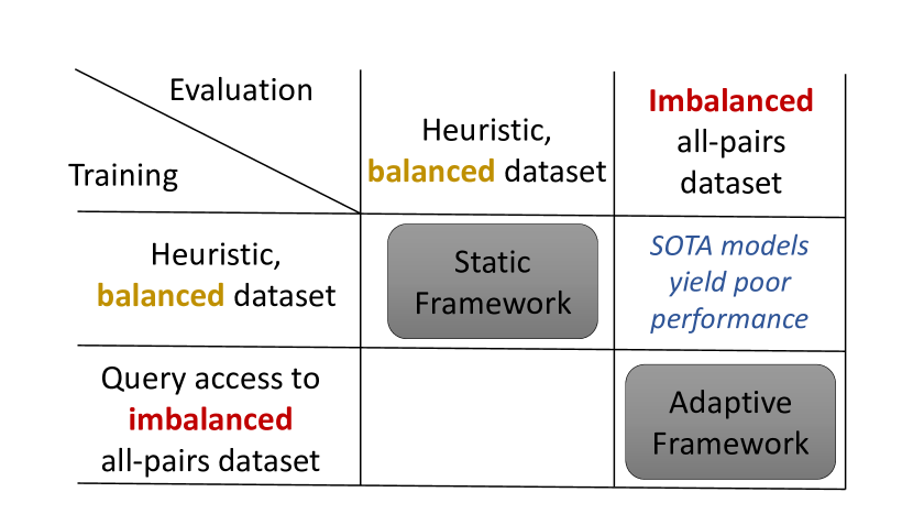
Figure 1: Modern benchmarks often use heuristically balanced data for training and evaluation. We find that models trained on this data perform poorly on the very imbalanced all-pairs distribution and develop adaptive methods to collect training data for this setting.

Instead of heuristically producing static training datasets, we study adaptive data collection methods. In particular, we apply the pool-based active learning framework (Settles, 2009) to extremely imbalanced pairwise tasks. At training time, the system has query access (i.e., the ability to collect a limited subset of the labels) to a large unlabeled dataset formed by taking all utterance pairs from a set of training utterances. For example, in the question deduplication setting, we might have a budget to annotate pairs of questions as “duplicate” or “not duplicate,” and wish to train a model on this data to find new duplicate pairs with high precision.

Data collection for extremely imbalanced pairwise tasks is challenging because the pool of unlabeled examples is very large (as it grows quadratically in the number of utterances) and very few of the examples are positive. We collect balanced training data using uncertainty sampling, an adaptive method that queries labels for examples on which a model trained on previously queried data has high uncertainty (Lewis and Gale, 1994). To lower the computational cost of searching for uncertain points, we propose combining active learning with a BERT embedding model for which uncertain points can be located efficiently using nearest neighbor search.

In this work, we empirically show that our use of adaptive data collection yields significant gains over static heuristics. In order to compare methods without collecting data separately for each method and each run, we perform retrospective data collection with imputed labels to simulate data collection. Uncertainty sampling with our BERT embedding model achieves $32.5\%$ and $20.1\%$ average precision for QQP and WikiQA, respectively. In contrast, state-of-the-art models trained on the original heuristically collected data each have only average precision of $2.4\%$.

2 Setting

The pairwise tasks described above fall under a more general category of binary classification tasks, those with an input space $\mathcal{X}$ and output space $\{0,1\}$. We assume the label $y$ is a deterministic function of $x$, which we write $y(x)$. A classification model $p_{\theta}$ yields probability estimates $p_{\theta}(y\mid x)$ where $x\in\mathcal{X}$.

Our setting has two aspects: The way training data is collected via label queries (Section 2.1) and the way we evaluate the model $p_{\theta}(y\mid x)$ by measuring average precision (Section 2.2). This work focuses on pairwise tasks (Section 2.3), which enables efficient active learning (Section 4).

2.1 Data collection

In our setting, a system is given an unlabeled dataset $D^{\text{train}}_{\text{all}}\subseteq\mathcal{X}$. The system can query an input $x\in D^{\text{train}}_{\text{all}}$ and receive the corresponding label $y(x)$. The system is given a budget of $n$ queries to build a labeled training dataset of size $n$.

2.2 Evaluation

Following standard practice for imbalanced tasks, we evaluate on precision, recall, and average precision (Lewis, 1995; Manning et al., 2008). A scoring function $S:\mathcal{X}\rightarrow\mathbb{R}$ (e.g., $S(x)=p_{\theta}(y=1\mid x)$) is used to rank examples $x$, where an ideal $S$ assigns all positive examples $\{x:y(x)=1\}$ a higher score than all negative examples $\{x:y(x)=0\}$. Given a test dataset $D^{\text{test}}_{\text{all}}\subseteq\mathcal{X}$, define the number of true positives, false positives, and false negatives of a scoring function $S$ at a threshold $\gamma$ as:

$$\text{TP}(S,\gamma) =\sum_{x\in D^{\text{test}}_{\text{all}}}\textbf{1}[y(x)=1\wedge S(x)\geq\gamma]$$ (1)

$$\text{FP}(S,\gamma) =\sum_{x\in D^{\text{test}}_{\text{all}}}\textbf{1}[y(x)=0\wedge S(x)\geq\gamma]$$ (2)

$$\text{FN}(S,\gamma) =\sum_{x\in D^{\text{test}}_{\text{all}}}\textbf{1}[y(x)=1\wedge S(x)<\gamma].$$ (3)

For any threshold $\gamma$, define the precision $P(S,\gamma)$ and recall $R(S,\gamma)$ of a scoring function $S$ as:

$$\text{P}(S,\gamma) =\frac{\text{TP}(S,\gamma)}{\text{TP}(S,\gamma)+\text{FP}(S,\gamma)}$$ (4)

$$\text{R}(S,\gamma) =\frac{\text{TP}(S,\gamma)}{\text{TP}(S,\gamma)+\text{FN}(S,\gamma)}.$$ (5)

Let $\Gamma=\{S(x):x\in D^{\text{test}}_{\text{all}}\}$ be the set of scores of the dataset. By sweeping over all distinct values $\Gamma$ in descending order, we trace out the precision-recall curve. The area under the precision recall curve or average precision (AP) is defined as:

$$\text{AP}(S)=\sum_{i=1}^{|\Gamma|}(\text{R}(S,\gamma_{i})-\text{R}(S,\gamma_{i-1}))\text{P}(S,\gamma_{i}),$$ (6)

where $\gamma_{0}=\infty$ and $\gamma_{1}>\gamma_{2}>\dots\gamma_{|\Gamma|}$ and $\gamma_{i}\in\Gamma$.

Note that high precision requires very high accuracy when the task is extremely imbalanced. For example, if only one in $10,000$ examples in $D^{\text{test}}_{\text{all}}$ is positive and 50% precision at some recall is achieved, that implies 99.99% accuracy.

2.3 Pairwise tasks

In this work, we focus on “pairwise” tasks, meaning that the input space decomposes as $\mathcal{X}=\mathcal{X}_{1}\times\mathcal{X}_{2}$. For instance, $\mathcal{X}_{1}$ could be questions and $\mathcal{X}_{2}$ could be paragraphs for open-domain question answering, and $\mathcal{X}_{1}=\mathcal{X}_{2}$ could be questions for question deduplication. We create the unlabeled all-pairs training set $D^{\text{train}}_{\text{all}}$ by taking the cross product of a subset from $\mathcal{X}_{1}$ and a subset from $\mathcal{X}_{2}$. We follow the same procedure to form the all-pairs test set, $D^{\text{test}}_{\text{all}}$. As is standard practice, we ensure that the train and test all-pairs sets are disjoint.

Many pairwise tasks require high average precision on all-pairs test data. A question deduplication system must compare a new question with all previously asked questions to determine if a duplicate exists. An open-domain question-answering system must search through all available documents for one that answers the question. In both cases, the all-pairs distribution is extremely imbalanced, as the vast majority of pairs are negatives, while standard datasets are artificially balanced.

3 Results training on heuristic datasets

In this section, we show that state-of-the-art models trained on two standard pairwise classification datasets—QQP and WikiQA—do not generalize well to our extremely imbalanced all-pairs test data, which we create from an original dataset by imputing a negative label for all pairs that are not marked as positive. Both QQP and WikiQA were collected using static heuristics that attempt to find points $x\in\mathcal{X}$ that are more likely to be positive. These heuristics are necessary because uniformly sampling from $\mathcal{X}$ is impractical due to the label imbalance: if the proportion of positives is $10^{-4}$, then random sampling would have to label 10,000 examples on average to find one positive example. Standard models can achieve high test accuracy on test data collected with these heuristics, but fare poorly when evaluated on all-pairs data derived from the same data source (Section 3.2). Manual inspection confirms that these models often make surprising false positive errors (Section 3.3).

3.1 Experimental setup

3.1.1 Evaluation

We evaluate models on both heuristically balanced test data and our imbalanced all-pairs test data.

Heuristically balanced evaluation.

Let $D_{\text{pos}}$ denote the set of all positive examples, and $D_{\text{statedneg}}$ denote the set of stated negative examples—negative examples in the original heuristically collected dataset. We define the stated test dataset $D^{\text{test}}_{\text{heur}}$ as the pairs in the original balanced dataset that are also in our defined test dataset: $(D_{\text{pos}}\cup D_{\text{statedneg}})\cap D^{\text{test}}_{\text{all}}$. This is similar to the original QQP test data, but with a different train/test split. We use task-specific evaluation metrics described in the next section.

All-pairs evaluation.

All-pairs evaluation metrics depend on the label of every pair in $D^{\text{test}}_{\text{all}}$. We approximate these labels by imputing (possibly noisy) labels on all pairs using the available labeled data, as described in the next section. In Section 3.3, we manually label examples to confirm our results from this automatic evaluation.

Computing the number of false positives $\text{FP}(S,\gamma)$ requires enumerating all negative examples in $D^{\text{test}}_{\text{all}}$, which is too computationally expensive with our datasets. To get an unbiased estimate of $\text{FP}(S,\gamma)$, we could randomly subsample $D^{\text{test}}_{\text{all}}$, but the resulting estimator has high variance. We instead compute an unbiased estimator that uses importance sampling. In particular, we combine counts of errors on a set of “nearby negative” examples $D^{\text{test}}_{\text{near}}\subseteq D^{\text{test}}_{\text{all}}$, pairs of similar utterances on which we expect more false positives to occur, and random negatives $D^{\text{test}}_{\text{rand}}$ sampled uniformly from negatives in $D^{\text{test}}_{\text{all}}\setminus D^{\text{test}}_{\text{near}}$. Details are provided in Appendix A.2.

3.1.2 Datasets

Quora Question Pairs (QQP).

The task for QQP (Iyer et al., 2017) is to determine whether two questions are paraphrases. The non-paraphrase pairs in the dataset were chosen heuristically, e.g., by finding questions on similar topics. We impute labels on all question pairs by assuming that two questions are paraphrases if and only if they are equivalent under the transitive closure of the equivalence relation defined by the labeled paraphrase pairs. We randomly partition all unique questions into train, dev, and test splits, ensuring that no two questions that were paired (either in positive or negative examples) in the original dataset end up in different splits. Since every question is a paraphrase of itself, we define $D^{\text{train}}_{\text{all}}$ as the set of distinct pairs of questions from the training questions, and define $D^{\text{dev}}_{\text{all}}$ and $D^{\text{test}}_{\text{all}}$ analogously. For heuristically balanced evaluation, we report accuracy and F1 score on $D^{\text{test}}_{\text{heur}}$, as in Wang et al. (2019).

WikiQA.

The task for WikiQA (Yang et al., 2015) is to determine whether a question is answered by a given sentence. The dataset only includes examples that pair a question with sentences from a Wikipedia article believed to be relevant based on click logs. We impute labels by assuming that question-sentence pairs not labeled in the dataset are negative. We partition the questions into train, dev, and test, following the original question-based split of the dataset, and then take the direct product with the set of all sentences in the original dataset to form the train, dev, and test sets. For all WikiQA models, we prepend the title of the source article to the sentence to give the model information about the sentence’s origin, as in Lee et al. (2019).

For heuristically balanced evaluation, we report two evaluation metrics. Following standard practice, we report clean mean average precision (c-MAP), defined as MAP over “clean” test questions—questions that are involved in both a positive and negative example in $D^{\text{test}}_{\text{heur}}$ (Garg et al., 2020). We also report F1 score across all examples in $D^{\text{test}}_{\text{heur}}$ (a-F1), which unlike c-MAP considers the more realistic setting where questions may not be answerable given the available article. This introduces more label imbalance, as positives make up $6\%$ of $D^{\text{test}}_{\text{heur}}$ but $12\%$ of clean examples. The original WikiQA paper advocated a-F1 (Yang et al., 2015), but most subsequent papers do not report it (Shen et al., 2017; Yoon et al., 2019; Garg et al., 2020).

Split	Positives	Total pairs	Ratio	Stated Neg.	Nearby Neg.
QQP
Train	124,625	38B	1:300K	132,796	-
Dev	60,510	8.8B	1:150K	61,645	13.1M
Test	43,413	8.5B	1:190K	60,575	12.8M
WikiQA
Train	1,040	56M	1:53K	19,320	-
Dev	140	7.8M	1:56K	2,593	29,511
Test	293	17M	1:57K	5,872	63,136

Table 1: Statistics of our QQP and WikiQA splits.

Data statistics.

Table 1 shows dataset statistics. Models in this section are trained on the stated training dataset $D^{\text{train}}_{\text{heur}}\triangleq(D_{\text{pos}}\cup D_{\text{statedneg}})\cap D^{\text{train}}_{\text{all}}$, the set of all positives and heuristic negatives in the train split. For all-pairs evaluation, both QQP and WikiQA have extreme label imbalance: Positive examples make up between 1 in 50,000 (WikiQA) and 1 in 200,000 (QQP) of the test examples.

3.1.3 Models

We train four state-of-the-art models that use BERT-base (Devlin et al., 2019), XLNet-base (Yang et al., 2019), RoBERTa-base (Liu et al., 2019), and ALBERT-base-v2 (Lan et al., 2020), respectively. As is standard, all models receive as input the concatenation of $x_{1}$ and $x_{2}$ separated by a special token; we refer to these as concatenation-based (Concat) models. We train on binary cross-entropy loss for 2 epochs on QQP and 3 epochs on WikiQA, chosen to maximize dev all-pairs AP for RoBERTa. We report the average over three random seeds for training.

QQP	Heur. Balanced		All pairs
	Accuracy	F1	P@R20	AP
BERT	$82.5\%$	$77.3\%$	$3.0\%$	$2.4\%$
XLNet	$83.0\%$	$77.9\%$	$1.7\%$	$1.4\%$
RoBERTa	$84.4\%$	$80.2\%$	$2.5\%$	$2.0\%$
ALBERT	$79.6\%$	$73.0\%$	$3.5\%$	$1.9\%$
WikiQA	c-MAP	a-F1	P@R=20	AP
BERT	$79.9\%$	$45.9\%$	$6.5\%$	$2.4\%$
XLNet	$80.5\%$	$46.7\%$	$1.0\%$	$1.0\%$
RoBERTa	$84.6\%$	$53.6\%$	$3.4\%$	$2.3\%$
ALBERT	$78.2\%$	$41.8\%$	$0.7\%$	$0.9\%$

Table 2: State-of-the-art Concat models trained on heuristically collected data generalize to test data from the same distribution, but not to all-pairs data.

3.2 Evaluation results

As shown in Table 2, state-of-the-art models trained only on stated training data do well on heuristically balanced test data but poorly on the extremely imbalanced all-pairs test data. On QQP, the best model gets $80.2\%$ F1 on heuristically balanced test examples. However, on all-pairs test data, the best model can only reach $3.5\%$ precision at a modest $20\%$ recall. On WikiQA, our best c-MAP of $84.6\%$ is higher than the best previously reported c-MAP without using additional question-answering data, $83.6\%$ (Garg et al., 2020). However, on all-pairs test data, the best model gets $6.5\%$ precision at $20\%$ recall. All-questions F1 on heuristically balanced data is also quite low, with the best model only achieving $53.6\%$. Since a-F1 evaluates on a more imbalanced distribution than c-MAP, this further demonstrates that state-of-the-art models deal poorly with test-time label imbalance. Compared with a-F1, all-pairs evaluation additionally shows that models make many mistakes when evaluated on questions paired with less related sentences; these examples should be easier to identify as negatives, but are missing from $D^{\text{train}}_{\text{heur}}$.

QQP, ConcatBERT trained on $D^{\text{train}}_{\text{heur}}$

$x_{1}$: “How do I overcome seasonal affective disorder?”
$x_{2}:$“How do I solve puberty problem?”

 

$x_{1}$: “What will 10000 A.D be like?”

$x_{2}:$“Does not introduction of new Rs.2000 notes ease carrying black money in future?”

 

$x_{1}$: “Can a person with no Coding knowledge learn Machine learning?”

$x_{2}$: “How do I learn Natural Language Processing?”

 

WikiQA, ConcatBERT trained on $D^{\text{train}}_{\text{heur}}$

$x_{1}$: “where does limestone form?”

$x_{2}$: “Glacier cave . A glacier cave is a cave formed within the ice of a glacier .”

 

$x_{1}$: “what is gravy made of?”

$x_{2}$: “Amaretto. It is made from a base of apricot pits or almonds, sometimes both.”

 

Figure 2: Examples of confident false positives from the all-pairs test distribution for models trained on examples from the original QQP and WikiQA datasets. Bold highlights non-equivalent phrases.

3.3 Manual verification of imputed negatives

Our all-pairs evaluation results are based on automatically imputed negative labels, rather than the gold label evaluation metrics. To check the validity of our results, we manually labeled putative false positive errors—examples that our model labeled positively but for which the imputed label was negative—to more accurately estimate precision. We focused on the best QQP model and random seed combination on the development set, which got $8.2\%$ precision at $20\%$ recall. For this recall threshold, we manually labeled 50 randomly chosen putative false positives from $D^{\text{dev}}_{\text{near}}$, and 50 more from $D^{\text{dev}}_{\text{rand}}$. In $72\%$ and $92\%$ of cases, respectively, the imputed label was correct and the model was wrong. Extrapolating from these results, we estimate the true precision of the model to be $9.5\%$, still close to our original estimate of $8.2\%$. See Appendix A.3 for more details. For the remainder of the paper, we simply use the imputed labels, keeping in mind this may underestimate precision.

Figure 2 shows real false positive predictions at $20\%$ recall for the best QQP and WikiQA models. For QQP, models often make surprising errors on pairs of unrelated questions (first two examples), as well as questions that are somewhat related but distinct (third example). For WikiQA, models often predict a positive label when something in the sentence has the same type as the answer to the question, even if the sentence and question are unrelated. While these pairs seem easy to classify, the heuristically collected training data lacks coverage of these pairs, leading to poor generalization.

4 Active learning for pairwise tasks

As shown above, training on heuristically collected balanced data leads to low average precision on all pairs. How can we collect training data that leads to high average precision? We turn to active learning, in which new data is chosen adaptively based on previously collected data. Adaptivity allows us to ignore the vast majority of obvious negatives (unlike random sampling) and iteratively correct the errors of our model (unlike static data collection) by collecting more data around the model’s decision boundary.

4.1 Active learning

Formally, an active learning method takes in an unlabeled dataset $D^{\text{train}}_{\text{all}}\subseteq\mathcal{X}$. Data is collected in a series of $k>1$ rounds. For the $i^{th}$ round, we choose a batch $B_{i}\subseteq D^{\text{train}}_{\text{all}}$ of size $n_{i}$ and observe the outcome as the labels $\{(x,y(x)):x\in B_{i}\}$. The budget $n$ is the total number of points labeled, i.e., $n=\sum_{i=1}^{k}n_{i}$. This process is adaptive because we can choose batch $B_{i}$ based on the labels of the previous $i-1$ batches. Static data collection corresponds to setting $k=1$.

Uncertainty sampling.

The main active learning algorithm we use is uncertainty sampling (Lewis and Gale, 1994), which is simple, effective, and commonly used in practice (Settles, 2009). Uncertainty sampling first uses a static data collection method to select the seed set $B_{1}$. For the next $k-1$ rounds, uncertainty sampling trains a model on all collected data and chooses $B_{i}$ to be the $n_{i}$ unlabeled points in $D^{\text{train}}_{\text{all}}$ on which the model is most uncertain. For binary classification, the most uncertain points are the points where $p_{\theta}(y=1\mid x)$ is closest to $\frac{1}{2}$. Note that a brute force approach to finding $B_{i}$ requires evaluating $p_{\theta}$ on every example in $D^{\text{train}}_{\text{all}}$, which can be prohibitively expensive. In balanced settings, it suffices to choose the most uncertain point from a small random subset of $D^{\text{train}}_{\text{all}}$ (Ertekin et al., 2007); however, this strategy works poorly in extremely imbalanced settings, as a small random subset of $D^{\text{train}}_{\text{all}}$ is unlikely to contain any uncertain points. In Section 4.2, we address this computational challenge with a bespoke model architecture.

Adaptive retrieval.

We also use a related algorithm we call adaptive retrieval, which is like uncertainty sampling but queries the $n_{i}$ unlabeled points in $D^{\text{train}}_{\text{all}}$ with highest $p_{\theta}(y=1\mid x)$ (i.e., pairs the model is most confident are positive). Adaptive retrieval can be seen as greedily maximizing the number of positive examples collected.

4.2 Modeling and implementation

We now fully specify our approach by describing our model, how we find pairs in the unlabeled pool $D^{\text{train}}_{\text{all}}$ to query, and how we choose the seed set $B_{1}$. In particular, a key technical challenge is that the set of training pairs $D^{\text{train}}_{\text{all}}$ is too large to enumerate, as it grows quadratically. We therefore require an efficient way to locate the uncertain points in $D^{\text{train}}_{\text{all}}$. We solve this problem with a model architecture CosineBERT that enables efficient nearest neighbor search (Gillick et al., 2019).

4.2.1 Model

Given input $x=(x_{1},x_{2})$, CosineBERT embeds $x_{1}$ and $x_{2}$ independently and predicts $p_{\theta}(y=1\mid x)$ based on vector-space similarity. More precisely,

$$p_{\theta}(y=1\mid x)=\sigma\left(w\cdot\frac{e_{\theta}(x_{1})\cdot e_{\theta}(x_{2})}{\|e_{\theta}(x_{1})\|\|e_{\theta}(x_{2})\|}+b\right),$$ (7)

where $\sigma$ is the sigmoid function, $w>0$ and $b$ are learnable parameters, and $e_{\theta}:\mathcal{X}_{1}\cup\mathcal{X}_{2}\rightarrow\mathbb{R}^{d}$ is a learnable embedding function. In other words, we compute the cosine similarity of the embeddings of $x_{1}$ and $x_{2}$, and predict $y$ using a logistic regression model with cosine similarity as its only feature. We define $e_{\theta}$ as the final layer output of a BERT model (Devlin et al., 2019) mean-pooled across all tokens (Reimers and Gurevych, 2019). Gillick et al. (2019) used a similar model for entity linking.

4.2.2 Finding points to query

Next, we show how to choose the batch $B_{i}$ of points to query, given a model $p_{\theta}(y\mid x)$ trained on data from batches $B_{1},\dotsc,B_{i-1}$. Recall that uncertainty sampling chooses the points $x$ for which for which $p_{\theta}(y=1\mid x)$ is closest to $\frac{1}{2}$, and adaptive retrieval chooses the points $x$ with largest $p_{\theta}(y=1\mid x)$. Since the set of positives is very small compared to the size of $D^{\text{train}}_{\text{all}}$, the set of uncertain points can be found by finding points with the largest $p_{\theta}(y=1\mid x)$, thus filtering out the confident negatives, and then selecting the most uncertain from those.

To find points with largest $p_{\theta}(y=1\mid x)$, we leverage the structure of our model. Since $w>0$, $p_{\theta}(y=1\mid x)$ is increasing in the cosine similarity of $e_{\theta}(x_{1})$ and $e_{\theta}(x_{2})$. Therefore, it suffices to find pairs $(x_{1},x_{2})$ that are nearest neighbors in the embedding space defined by $e_{\theta}$. In particular, for each $x_{1}\in\mathcal{X}_{1}$, we use the Faiss library (Johnson et al., 2017) to retrieve a set $N(x_{1})$ containing the $m$ nearest neighbors in $\mathcal{X}_{2}$, and define $D^{\text{train}}_{\text{close}}$ to be the set of all pairs $(x_{1},x_{2})$ such that $x_{2}\in N(x_{1})$. We then iterate through $D^{\text{train}}_{\text{close}}$ to find either the most uncertain points (for uncertainty sampling) or points with highest cosine similarity (for adaptive retrieval). Note that this method only requires embedding the number of distinct elements that appear in the training set, rather than the total number of pairs, the requirement for jointly embedding all pairs.

4.2.3 Choosing the seed set

Recall that both of our active learning techniques require a somewhat representative initial seed set $B_{1}$ to start the process. We use the pre-trained BERT model as the embedding $e_{\theta}$ and select the $n_{1}$ pairs with largest $p_{\theta}(y=1\mid x)$. Recall that $w>0$, so this amounts to choosing the pairs with highest cosine similarity.

5 Active learning experiments

5.1 Experimental details

We simulate active learning with the imputed labels so that we can compare different algorithms without performing expensive gold label collection for each algorithm. We collect $n_{1}=2048$ examples in the seed set, and use $k=10$ rounds of active learning for QQP and $k=4$ for WikiQA, as WikiQA is much smaller. At round $i$, we query $n_{i}=n_{1}\cdot(3/2)^{i-1}$ new labels. The exponentially growing $n_{i}$ helps us avoid wasting queries in early rounds, when the model is worse, and also makes training faster in the early rounds. These choices imply a total labeling budget $n$ of 232,100 for QQP and 16,640 for WikiQA. For both datasets, $n$ is slightly less than $|D^{\text{train}}_{\text{heur}}|$ (257,421 for QQP and 20,360 for WikiQA), thus ensuring a meaningful comparison with training on heuristic data. We retrieve $m=1000$ nearest neighbors per $x_{1}\in\mathcal{X}_{1}$ for QQP and $m=100$ for WikiQA. We run all active learning experiments with three different random seeds and report the mean. Training details are given in Appendix A.

5.2 Main results

Method	QQP		WikiQA
	P@R20	AP	P@R20	AP
Random	$4.7\%$	$2.8\%$	$1.3\%$	$1.3\%$
Stated data	$29.3\%$	$15.4\%$	$0.7\%$	$2.2\%$
Static Ret.	$49.2\%$	$25.1\%$	$13.9\%$	$8.2\%$
Adapt. Ret.	$59.1\%$	$32.4\%$	$27.1\%$	$15.1\%$
Uncertainty	$\bf 60.2\%$	$\bf 32.5\%$	$\bf 32.4\%$	$\bf 20.1\%$

Table 3: Main results comparing different data collection strategies on QQP and WikiQA. The two active learning methods, adaptive retrieval and uncertainty sampling, greatly outperform other methods.

Positives Found	QQP	WikiQA
Random sampling	1	1
Static retrieval	16,422	169
Adaptive retrieval	103,181	757
Uncertainty sampling	87,594	742
Total examples collected	232,100	16,640

Table 4: Number of positive points collected by different methods. All methods collect the same number of total examples (last row).

We now compare the two active learning methods, adaptive retrieval and uncertainty sampling, with training on $D^{\text{train}}_{\text{heur}}$ and two other baselines. Random sampling queries $n$ pairs uniformly at random, which creates a very imbalanced dataset. Static retrieval queries the $n$ most similar pairs using the pre-trained BERT embedding, similar to Section 4.2.3. Table 3 shows all-pairs evaluation for CosineBERT trained on these datasets. The two active learning methods greatly outperform other methods: Uncertainty sampling gets $32.5\%$ AP on QQP and $20.1\%$ on WikiQA, while the best static data collection method, static retrieval, gets only $25.1\%$ AP on QQP and $8.2\%$ AP on WikiQA. Recall from Table 2 that ConcatBERT only achieved $2.4\%$ AP on both QQP and WikiQA. When trained on the same data as ConcatBERT, CosineBERT achieves much higher AP on QQP ($15.4\%$) but slightly lower AP on WikiQA ($2.2\%$). Uncertainty sampling slightly outperforms adaptive retrieval on both datasets.

Achieving high precision across all pairs requires collecting both enough positive examples and useful negative examples. Compared to random sampling and static retrieval, active learning collects many more positive examples, as shown in Table 4. $D^{\text{train}}_{\text{heur}}$ contains all positive examples, but models trained on it still have low AP on all pairs. We conclude that the negative examples in $D^{\text{train}}_{\text{heur}}$ are insufficient for generalization to all pairs, while active learning chooses more useful negatives.

5.3 Manual verification of imputed negatives

As in Section 3.3, we manually labeled putative QQP false positives at the threshold where recall is $20\%$ for CosineBERT trained on either stated data or uncertainty sampling data. For each, we labeled 50 putative false positives from $D^{\text{dev}}_{\text{near}}$, and all putative false positives from $D^{\text{dev}}_{\text{rand}}$ (12 for stated data, 0 for uncertainty sampling).

CosineBERT trained on $D^{\text{train}}_{\text{heur}}$.

$67\%$ (8 of 12) of the putative false positives on $D^{\text{dev}}_{\text{rand}}$ were actual errors by the model, but only $36\%$ of putative false positives on $D^{\text{dev}}_{\text{near}}$ were errors. Extrapolating from these results, we update our estimate of development set precision at $20\%$ recall from $28.4\%$ to $41.4\%$.

Overall, this model makes some more reasonable mistakes than the ConcatBERT model, though its precision is still not that high.

CosineBERT model with uncertainty sampling.

Only $32\%$ of putative false positives from $D^{\text{dev}}_{\text{near}}$ were real errors, significantly less than the $72\%$ for ConcatBERT trained on $D^{\text{train}}_{\text{heur}}$ ($p=7\times 10^{-5}$, Mann-Whitney U test). Extrapolating from these results, we update our estimate of development set precision at $20\%$ recall from $55.1\%$ to $79.3\%$, showing that uncertainty sampling yields a more precise model than our imputed labels indicate. In fact, this model provides a high-precision way to identify paraphrase pairs not annotated in the original dataset.

5.4 Comparison with stratified sampling

Method	QQP		WikiQA
	P@R20	AP	P@R20	AP
Strat. match	$35.1\%$	$19.0\%$	$13.2\%$	$8.5\%$
Strat. all pos.	$41.6\%$	$22.2\%$	$13.7\%$	$9.1\%$
Adapt. Ret.	$59.1\%$	$32.4\%$	$27.1\%$	$15.1\%$
Uncertainty	$\bf 60.2\%$	$\bf 32.5\%$	$\bf 32.4\%$	$\bf 20.1\%$

Table 5: Even though stratified sampling has access to oracle information, active learning performs better by collecting more informative negative examples.

Next, we further confirm that having all the positive examples is not sufficient for high precision. In Table 5, we compare with two variants of stratified sampling, in which positive and negative examples are independently subsampled at a desired ratio (Attenberg and Provost, 2010). First, we randomly sample positive and negative training examples to match the number of positives and negatives collected by uncertainty sampling, the best active learning method for both datasets (“Strat. match” in Table 5). Second, we trained on all positive examples and added negatives to match the number of positives on QQP or match the active learning total budget on WikiQA (“Strat. all pos.”). For QQP, this yielded a slightly larger dataset than the first setting. Note that stratified sampling requires oracle information: It assumes the ability to sample uniformly from all positives, even though this set is not known before data collection begins. Nonetheless, stratified sampling trails uncertainty sampling by more than $10$ AP points on both datasets. Since stratified sampling has access to all positives, active learning must be choosing more informative negative examples.

5.5 Training other models on collected data

QQP Data	CosineBERT		ConcatBERT
	P@R20	AP	P@R20	AP
Stated data	$29.3\%$	$15.4\%$	$3.0\%$	$2.4\%$
Static Ret.	$49.2\%$	$25.1\%$	$4.6\%$	$1.9\%$
Stratified	$35.1\%$	$19.0\%$	$29.0\%$	$16.4\%$
Uncertainty	$\bf 60.2\%$	$\bf 32.5\%$	$23.6\%$	$8.9\%$

Table 6: Comparison on QQP of CosineBERT with ConcatBERT. Data collected by active learning (using CosineBERT) is more useful for training ConcatBERT than stated data or static retrieval data. Stratified sampling here matches the label balance of the uncertainty sampling data.

For QQP, data collected with active learning and CosineBERT is useful for training other models on the same task. Table 6 shows that ConcatBERT does better on data collected by active learning—using CosineBERT—compared to the original dataset or static retrieval. ConcatBERT performs best with stratified sampling; recall that this is not a comparable data collection strategy in our setting, as it requires oracle knowledge. CosineBERT outperforms ConcatBERT in all training conditions; we hypothesize that the cosine similarity structure helps it generalize more robustly to pairs of unrelated questions. However, CosineBERT trained on stated data does not do as well on WikiQA, as shown in Table 3.

5.6 Data efficiency

Adaptivity is crucial for getting high AP with less labeled data. Static retrieval, the best static data collection method, gets $21.9\%$ dev AP on QQP with the full budget of 232,100 examples. Uncertainty sampling achieves a higher dev AP of $22.6\%$ after collecting only 16,640 examples, for a $14\times$ data efficiency improvement. See Appendix B.1 for further analysis.

5.7 Effect of seed set

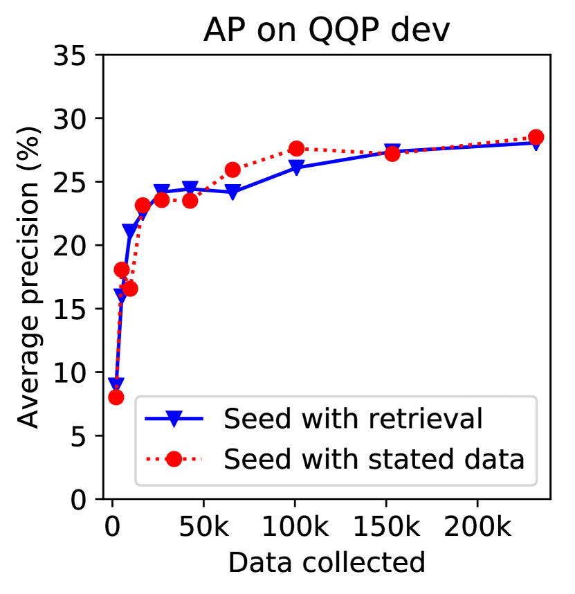
(a) Average precision

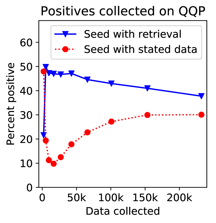
(b) Positives collected

Figure 3: Uncertainty sampling on QQP using different seed sets. (a) Seeding with stated data (one run) does similarly to seeding with retrieval (mean over three runs). (b) Seeding with stated data makes the model poorly calibrated—points it is uncertain about are initially very unlikely to be positive. However, over time the model corrects this behavior.

Our method is robust to choice of the initial seed set for uncertainty sampling. We consider using stated data as the seed set, instead of data chosen via static retrieval. As shown in Figure 3, seeding with stated data performs about as well as static retrieval in terms of AP. Since the stated data artificially overrepresents positive examples, the model trained on stated data is initially miscalibrated—the points it is uncertain about are actually almost all negative points. Therefore, uncertainty sampling initially collects very few additional positive examples. Over time, adaptively querying new data helps correct for this bias.

6 Discussion and related work

In this paper, we have studied how to collect training data that enables generalization to extremely imbalanced test data in pairwise tasks. State-of-the-art models trained on standard, heuristically collected datasets have very low average precision when evaluated on imbalanced test data, while active learning leads to much better average precision.

Gillick et al. (2019) propose a similar model for entity linking and mine hard negative examples, an approach related to adaptive retrieval. However, they have abundant labeled data, whereas we study data collection with a limited labeling budget.

Work in information retrieval often attempts to maximize precision across all pairs of test objects. Machine learning models are commonly used to re-rank candidate pairs from an upstream retriever (Chen et al., 2017; Nogueira and Cho, 2019), while our method learns embeddings to improve the initial retrieval step. Distant supervision has been used to train end-to-end retrieval models for question answering (Lee et al., 2019), but does not extend to other tasks like paraphrase detection. Other work on duplicate question detection on community QA forums trains on labels generated by forum users (dos Santos et al., 2015). Hoogeveen et al. (2016) show that these datasets tend to have many false negatives and suggests additional labeling to correct this problem; active learning provides one way to choose informative pairs to label.

Extreme label imbalance is an important challenge in many non-pairwise NLP tasks, including document classification (Lewis et al., 2004) and relation extraction (Zhang et al., 2017). Most prior work focuses on sampling a fixed training dataset (Chawla et al., 2004; Sun et al., 2009; Dendamrongvit and Kubat, 2009), whereas our work explores data collection. Attenberg and Provost (2010) find stratified sampling outperforms active learning in non-pairwise imbalanced tasks, primarily due to the difficulty of finding a useful seed set. We find pre-trained embeddings effective for seed set collection in pairwise tasks.

Zhang et al. (2019) found that the frequency of questions in QQP leaks information about the label. Evaluating on all pairs avoids such artifacts, as every test utterance appears in the same number of examples. Zhang et al. (2019) re-weight the original dataset to avoid these biases, but re-weighting cannot compensate for the absence of some types of negative examples, unlike active learning.

Many pairwise datasets are generated by asking crowdworkers to generate part or all of the input $x$ (Bowman et al., 2015; Mostafazadeh et al., 2016). Having crowdworkers generate text increases the risk of introducing artifacts (Schwartz et al., 2017; Poliak et al., 2018), while our pool-based approach considers the entire distribution of utterance pairs.

We use active learning, specifically uncertainty sampling Lewis and Gale (1994), to create a balanced training set that leads to models that generalize to the full imbalanced distribution. Ertekin et al. (2007) argues that active learning is capable of providing balanced classes to the learning algorithm by selecting examples close to the decision boundary. Furthermore, active learning can generalize to the full distribution, both empirically (Settles, 2009; Yang and Loog, 2018) and theoretically (Balcan et al., 2007; Balcan and Long, 2013; Mussmann and Liang, 2018).

Finally, this paper addresses two central concerns in NLP today: How to construct fair but challenging tests of generalization (Geiger et al., 2019), and how to collect training data in a way that improves generalization. Evaluating on extremely imbalanced all-pairs data has several advantages over other tests of generalization. Our examples are realistic and natural, unlike adversarial perturbations (Ebrahimi et al., 2018; Alzantot et al., 2018), and diverse, unlike hand-crafted tests of specific phenomena (Glockner et al., 2018; Naik et al., 2018; McCoy et al., 2019). Since we allow querying the label of any training example, generalization to our test data is achievable, while out-of-domain generalization (Levy et al., 2017; Yogatama et al., 2019; Talmor and Berant, 2019) may be statistically impossible. Our work thus offers a natural, challenging, and practically relevant testbed to study both generalization and data collection.

Reproducibility.

Code and data needed to reproduce all results can be found on the CodaLab platform at https://bit.ly/2GzJAgM.

Appendix A Experimental details

A.1 Training details

At each round of active learning, we train for $2$ epochs. We train without dropout, as dropout artificially lowers cosine similarities at training time. We apply batch normalization (Ioffe and Szegedy, 2015) to the cosine similarity layer to rescale the cosine similarities, as they often are very close to 1. We initialize $w$ and $b$ so that high cosine similarities correspond to the positive label, and constrain $w$ to be nonnegative during training. We use a maximum sequence length of 128 word piece tokens. To compensate for BERT’s low learning rate, we increased the learning rate on the $w$ and $b$ parameters by a factor of $10^{4}$.

Below in Table 7, we show hyperparameters for training. Hyperparameters were tuned on the development set of QQP; we found these same hyperparameters also worked well for WikiQA, and so we did not tune them separately for WikiQA. In most cases, we used the default hyperparameters for BERT.

Hyperparameter	Value
Learning rate	$2\times 10^{-5}$
Training epochs	2
Weight decay	$0$
Optimizer	AdamW
AdamW Epsilon	$1\times 10^{-6}$
Batch size	16

Table 7: Hyperparameter choices for QQP and WikiQA

At the end of training, we freeze the embeddings $e_{\theta}$ and train the output layer parameters $w$ and $b$ to convergence, to improve uncertainty estimates for uncertainty sampling. This process amounts to training a two-parameter logistic regression model. We optimize this using (batch) gradient descent with learning rate $1$ and $10,000$ iterations. When training this model, we normalize the cosine similarity feature to have zero mean and unit variance across the training dataset. Training this was very fast compared to running the embedding model.

Each experiment was conducted with a single GPU, most commonly a TITAN V or TITAN Xp. Running one complete uncertainty sampling experiment (i.e., 10 rounds of data collection and model training for QQP, 4 for WikiQA) on a machine with one TITAN V GPU takes about 9 hours for QQP and about 30 minutes for WikiQA. Recall that CosineBERT only adds two additional parameters, $w$ and $b$, on top of a BERT model; we use the uncased BERT-base pre-trained model which has 110M parameters.

A.2 Evaluation details

To evaluate a given scoring function $S$ at threshold $\gamma$ on a test set $D^{\text{test}}_{\text{all}}$, we must compute the number of true positives $\text{TP}(S,\gamma)$, false positives $\text{FP}(S,\gamma)$, and false negatives $\text{FN}(S,\gamma)$. True positives and false negatives are computationally easy to compute, as they only require evaluating $S(x)$ on all the positive inputs $x$ in $D^{\text{test}}_{\text{all}}$. However, without any structural assumptions on $S$, it is computationally infeasible to exactly compute the number of false positives, as that would require evaluating $S$ on every negative example in $D^{\text{test}}_{\text{all}}$, which is too large to enumerate.

Therefore, we devise an approach to compute an unbiased, low-variance estimate of $\text{FP}(S,\gamma)$. Recall that this term is defined as

$$\text{FP}(S,\gamma) =\sum_{x\in D^{\text{test}}_{\text{all}}}\textbf{1}[y(x)=0\wedge S(x)>\gamma]$$ (8)

$$=\sum_{x\in D^{\text{test}}_{\text{neg}}}\textbf{1}[S(x)>\gamma]$$ (9)

where $D^{\text{test}}_{\text{neg}}$ denotes the set of all negative examples in $D^{\text{test}}_{\text{all}}$.

One approach to estimating $\text{FP}(S,\gamma)$ would be simply to randomly subsample $D^{\text{test}}_{\text{neg}}$ to some smaller set $R$, count the number of false positives in $R$, and then multiply the count by $|D^{\text{test}}_{\text{neg}}|/|R|$. This would be an unbiased estimate of $D^{\text{test}}_{\text{neg}}$, but has high variance when the rate of false positive errors is low. For example, if $|D^{\text{test}}_{\text{neg}}|=10^{10}$, $|R|=10^{6}$, and the model makes a false positive error on $1$ in $10^{6}$ examples in $D^{\text{test}}_{\text{neg}}$, then $\text{FP}(S,\gamma)=10^{4}$. However, with probability

$$\left(1-\frac{1}{10^{6}}\right)^{10^{6}}\approx 1/e\approx 0.368,$$

$R$ will contain no false positives, so we will estimate $\text{FP}(S,\gamma)$ as $0$. A similar calculation shows that the probability of having exactly one false positive in $R$ is also roughly $1/e$, which means that with probability roughly $1-2/e\approx 0.264$, we will have at least two false positives in $R$, and therefore overestimate $\text{FP}(S,\gamma)$ by at least a factor of two.

To get a lower variance estimate $\hat{\text{FP}}(S,\gamma)$, we preferentially sample from likely false positives and use importance weighting to get an unbiased estimate of $\text{FP}(S,\gamma)$. In particular, we construct $D^{\text{test}}_{\text{near}}$ to be the pairs in $D^{\text{test}}_{\text{all}}$ with nearby pre-trained BERT embeddings, analogously to how we create the seed set in Section 4.2.3. Points with nearby BERT embeddings are likely to look similar are therefore more likely to be false positives. Note that

$$\text{FP}(S,\gamma) =\sum_{x\in D^{\text{test}}_{\text{near}}}\textbf{1}[S(x)>\gamma]$$

$$+\sum_{x\in D^{\text{test}}_{\text{neg}}\setminus D^{\text{test}}_{\text{near}}}\textbf{1}[S(x)>\gamma]$$ (10)

$$=\sum_{x\in D^{\text{test}}_{\text{near}}}\textbf{1}[S(x)>\gamma]$$

$$+w_{\text{rand}}\cdot\mathbb{E}_{x\sim\text{Unif}(D^{\text{test}}_{\text{neg}}\setminus D^{\text{test}}_{\text{near}})}\textbf{1}[S(x)>\gamma],$$ (11)

where we define $w_{\text{rand}}=|D^{\text{test}}_{\text{neg}}|-|D^{\text{test}}_{\text{near}}|$.

We can compute the first term exactly, since $D^{\text{test}}_{\text{near}}$ is small enough to enumerate, and approximate the second term as

$$w_{\text{rand}}\cdot\frac{1}{|D^{\text{test}}_{\text{rand}}|}\sum_{x\in D^{\text{test}}_{\text{rand}}}\textbf{1}[S(x)>\gamma],$$ (12)

where $D^{\text{test}}_{\text{rand}}$ is a uniformly random subset of $D^{\text{test}}_{\text{neg}}\setminus D^{\text{test}}_{\text{near}}$. Therefore, our final estimate is

$$\hat{\text{FP}}(S,\gamma) =\sum_{x\in D^{\text{test}}_{\text{near}}}\textbf{1}[S(x)>\gamma]$$

$$+\frac{w_{\text{rand}}}{|D^{\text{test}}_{\text{rand}}|}\sum_{x\in D^{\text{test}}_{\text{rand}}}\textbf{1}[S(x)>\gamma].$$ (13)

A.3 Incorporating manual labels

In Section 3.3, we manually label examples that were automatically labeled as false positives, and use this to improve our estimates of the true model precision. We manually label randomly chosen putative false positives from both $D^{\text{dev}}_{\text{near}}$ and $D^{\text{dev}}_{\text{rand}}$, and use this to estimate the proportion of putative false positives in each set that are real false positives. Let $\hat{p}_{\text{near}}$ denote the estimated fraction of putative false positives in $D^{\text{dev}}_{\text{near}}$ that are real false positives, and $\hat{p}_{\text{rand}}$ be the analogous quantity for $D^{\text{dev}}_{\text{rand}}$. Our updated estimate $\hat{\text{FP}}_{\text{manual}}(S,\gamma)$ is then defined as

$$\hat{\text{FP}}_{\text{manual}}(S,\gamma) =\hat{p}_{\text{near}}\sum_{x\in D^{\text{test}}_{\text{near}}}\textbf{1}[S(x)>\gamma]$$

$$+\frac{\hat{p}_{\text{random}}\cdot w_{\text{rand}}}{|D^{\text{test}}_{\text{rand}}|}\sum_{x\in D^{\text{test}}_{\text{rand}}}\textbf{1}[S(x)>\gamma].$$ (14)

We then compute precision using $\hat{\text{FP}}_{\text{manual}}(S,\gamma)$ in place of $\hat{\text{FP}}(S,\gamma)$.

A.4 Comparison with GLUE QQP data

For a few reasons, our QQP in-domain accuracy numbers are lower than those on the GLUE leaderboard, which has accuracies in the low $90$’s. First, our training set is smaller (257K examples versus 364K). Second, our split is more challenging because the model does not see the same questions or even same paraphrase clusters at training time and test time. Finally, our test set is more balanced ($58\%$ negative) than the GLUE QQP dev set ($63\%$ negative; test set balance is unknown). As a sanity check, we confirmed that our RoBERTa implementation can achieve $91.5\%$ dev accuracy when trained and tested on the GLUE train/dev split, in line with previously reported results (Liu et al., 2019).

Appendix B Additional experimental results

B.1 Learning curves and data efficiency

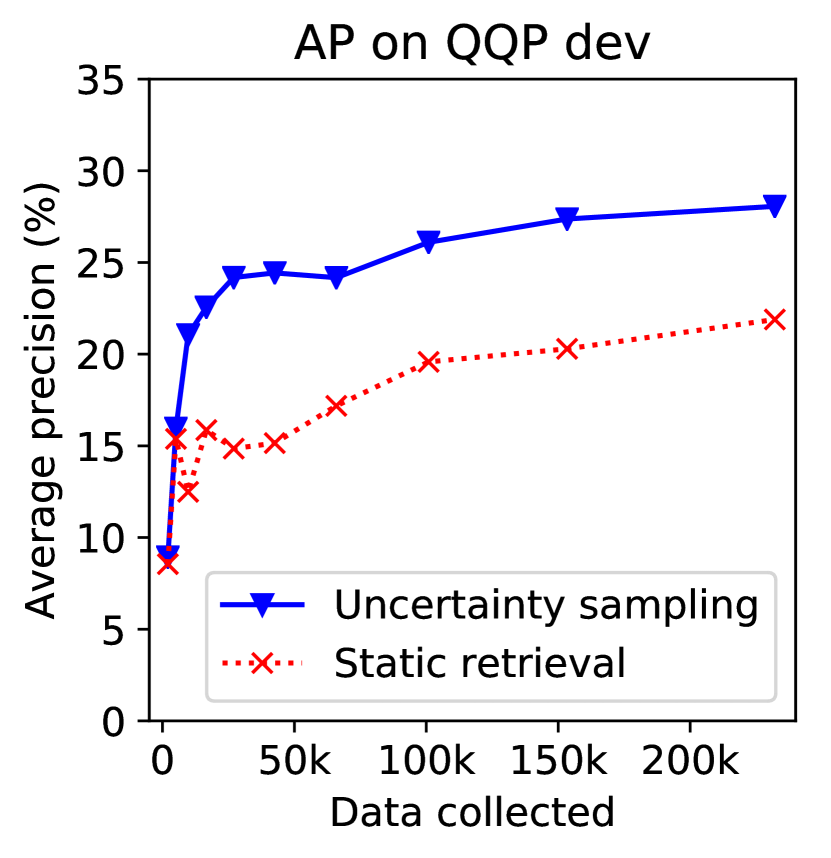
(a) Average precision

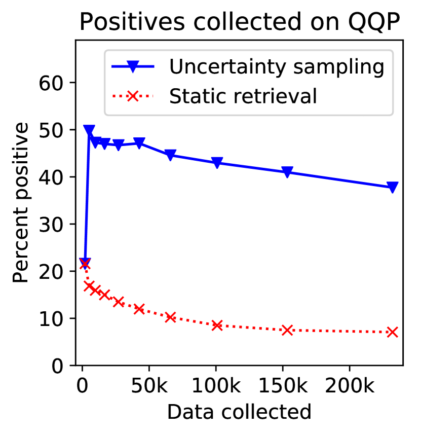
(b) Positives collected

Figure 4: Uncertainty sampling compared with matching amounts of static retrieval data on QQP. (a) Average precision is higher for uncertainty sampling. (b) Percent of all collected data that is positive. Adaptivity helps uncertainty sampling collect more positives.

In Figure 4(a), we plot average precision on the QQP dev set for our model after each round of uncertainty sampling. For comparison, we show a model trained on the same amount of data collected via static retrieval, the best-performing static data collection method. Uncertainty sampling leads to higher AP with much less data. For example, uncertainty sampling only needs to collect 16,640 examples to surpass the average precision of static retrieval collecting all 232,100 examples, for a $14\times$ data efficiency improvement. A big factor for the success of uncertainty sampling is its ability to collect many more positive examples than static retrieval, as shown in Figure 4(b). Static retrieval collects fewer positives over time, as it exhausts the set of positives that are easy to identify. However, uncertainty sampling collects many more positives, especially after the first round of training, because it improves its embeddings over time.

References

- Alzantot et al. (2018) M. Alzantot, Y. Sharma, A. Elgohary, B. Ho, M. Srivastava, and K. Chang. 2018. Generating natural language adversarial examples. In Empirical Methods in Natural Language Processing (EMNLP).
- Attenberg and Provost (2010) J. Attenberg and F. Provost. 2010. Why label when you can search? alternatives to active learning for applying human resources to build classification models under extreme class imbalance. In International Conference on Knowledge Discovery and Data Mining (KDD).
- Balcan et al. (2007) Maria-Florina Balcan, Andrei Broder, and Tong Zhang. 2007. Margin based active learning. In International Conference on Computational Learning Theory, pages 35–50. Springer.
- Balcan and Long (2013) Maria-Florina Balcan and Phil Long. 2013. Active and passive learning of linear separators under log-concave distributions. In Conference on Learning Theory, pages 288–316.
- Bowman et al. (2015) S. Bowman, G. Angeli, C. Potts, and C. D. Manning. 2015. A large annotated corpus for learning natural language inference. In Empirical Methods in Natural Language Processing (EMNLP).
- Chawla et al. (2004) N. V. Chawla, N. Japkowicz, and A. R. Kolcz. 2004. Editorial: Special issue on learning from imbalanced data sets. ACM SIGKDD Explorations Newsletter, 6(1).
- Chen et al. (2017) D. Chen, A. Fisch, J. Weston, and A. Bordes. 2017. Reading Wikipedia to answer open-domain questions. In Association for Computational Linguistics (ACL).
- Dendamrongvit and Kubat (2009) S. Dendamrongvit and M. Kubat. 2009. Undersampling approach for imbalanced training sets and induction from multi-label text-categorization domains. In PAKDD Workshop on New Frontiers in Applied Data Mining.
- Devlin et al. (2019) J. Devlin, M. Chang, K. Lee, and K. Toutanova. 2019. BERT: Pre-training of deep bidirectional transformers for language understanding. In Association for Computational Linguistics (ACL), pages 4171–4186.
- dos Santos et al. (2015) C. dos Santos, L. Barbosa, D. Bogdanova, and B. Zadrozny. 2015. Learning hybrid representations to retrieve semantically equivalent questions. In Association for Computational Linguistics (ACL).
- Ebrahimi et al. (2018) J. Ebrahimi, A. Rao, D. Lowd, and D. Dou. 2018. Hotflip: White-box adversarial examples for text classification. In Association for Computational Linguistics (ACL).
- Ertekin et al. (2007) Seyda Ertekin, Jian Huang, Leon Bottou, and Lee Giles. 2007. Learning on the border: active learning in imbalanced data classification. In Proceedings of the sixteenth ACM conference on Conference on information and knowledge management, pages 127–136.
- Garg et al. (2020) S. Garg, T. Vu, and A. Moschitti. 2020. TANDA: Transfer and adapt pre-trained transformer models for answer sentence selection. In Association for the Advancement of Artificial Intelligence (AAAI).
- Geiger et al. (2019) A. Geiger, I. Cases, L. Karttunen, and C. Potts. 2019. Posing fair generalization tasks for natural language inference. In Empirical Methods in Natural Language Processing (EMNLP).
- Gillick et al. (2019) D. Gillick, S. Kulkarni, L. Lansing, A. Presta, J. Baldridge, E. Ie, and D. Garcia-Olano. 2019. Learning dense representations for entity retrieval. In Computational Natural Language Learning (CoNLL).
- Glockner et al. (2018) M. Glockner, V. Shwartz, and Y. Goldberg. 2018. Breaking NLI systems with sentences that require simple lexical inferences. In Association for Computational Linguistics (ACL).
- Harman (1992) D. K. Harman. 1992. Overview of the first TREC text retrieval conference. In Text Retrieval Conference.
- Hoogeveen et al. (2016) D. Hoogeveen, Karin M. Verspoor, and Timothy Baldwin. 2016. Cqadupstack: Gold or silver? In SIGIR 2016 Workshop on Web Question Answering Beyond Factoids (WebQA 2016).
- Ioffe and Szegedy (2015) S. Ioffe and C. Szegedy. 2015. Batch normalization: Accelerating deep network training by reducing internal covariate shift. In International Conference on Machine Learning (ICML), pages 448–456.
- Iyer et al. (2017) Shankar Iyer, Nikhil Dandekar, and Kornél Csernai. 2017. First quora dataset release: Question pairs. https://www.quora.com/q/quoradata/First-Quora-Dataset-Release-Question-Pairs.
- Ji et al. (2011) H. Ji, R. Grishman, and H. Trang Dang. 2011. Overview of the TAC 2011 knowledge base population track. In Text Analytics Conference.
- Johnson et al. (2017) Jeff Johnson, Matthijs Douze, and Hervé Jégou. 2017. Billion-scale similarity search with gpus. arXiv preprint arXiv:1702.08734.
- Lan et al. (2020) Z. Lan, M. Chen, S. Goodman, K. Gimpel, P. Sharma, and R. Soricut. 2020. ALBERT: A lite BERT for self-supervised learning of language representations. In International Conference on Learning Representations (ICLR).
- Lee et al. (2019) K. Lee, M. Chang, and K. Toutanova. 2019. Latent retrieval for weakly supervised open domain question answering. In Association for Computational Linguistics (ACL).
- Levy et al. (2017) O. Levy, M. Seo, E. Choi, and L. Zettlemoyer. 2017. Zero-shot relation extraction via reading comprehension. In Computational Natural Language Learning (CoNLL).
- Lewis (1995) D. D. Lewis. 1995. Evaluating and optimizing autonomous text classification systems. In ACM Special Interest Group on Information Retreival (SIGIR).
- Lewis et al. (2004) D. D. Lewis, Y. Yang, T. G. Rose, and F. Li. 2004. Rcv1: A new benchmark collection for text categorization research. Journal of Machine Learning Research (JMLR), 5.
- Lewis and Gale (1994) David D Lewis and William A Gale. 1994. A sequential algorithm for training text classifiers. In SIGIR’94, pages 3–12. Springer.
- Liu et al. (2019) Y. Liu, M. Ott, N. Goyal, J. Du, M. Joshi, D. Chen, O. Levy, M. Lewis, L. Zettlemoyer, and V. Stoyanov. 2019. RoBERTa: A robustly optimized BERT pretraining approach. arXiv preprint arXiv:1907.11692.
- Manning et al. (2008) C. Manning, P. Raghavan, and H. Schütze. 2008. Introduction to information retrieval, volume 1. Cambridge University Press.
- McCoy et al. (2019) R. T. McCoy, E. Pavlick, and T. Linzen. 2019. Right for the wrong reasons: Diagnosing syntactic heuristics in natural language inference. In Association for Computational Linguistics (ACL).
- Mostafazadeh et al. (2016) N. Mostafazadeh, N. Chambers, X. He, D. Parikh, D. Batra, L. Vanderwende, P. Kohli, and J. Allen. 2016. A corpus and cloze evaluation for deeper understanding of commonsense stories. In North American Association for Computational Linguistics (NAACL).
- Mussmann and Liang (2018) Stephen Mussmann and Percy S Liang. 2018. Uncertainty sampling is preconditioned stochastic gradient descent on zero-one loss. In Advances in Neural Information Processing Systems, pages 6955–6964.
- Naik et al. (2018) A. Naik, A. Ravichander, N. Sadeh, C. Rose, and G. Neubig. 2018. Stress test evaluation for natural language inference. In International Conference on Computational Linguistics (COLING), pages 2340–2353.
- Nogueira and Cho (2019) R. Nogueira and K. Cho. 2019. Passage re-ranking with BERT. arXiv preprint arXiv:1901.04085.
- Poliak et al. (2018) A. Poliak, J. Naradowsky, A. Haldar, R. Rudinger, and B. V. Durme. 2018. Hypothesis only baselines in natural language inference. arXiv preprint arXiv:1805.01042.
- Reimers and Gurevych (2019) N. Reimers and I. Gurevych. 2019. Sentence-BERT: Sentence embeddings using siamese BERT-networks. In Empirical Methods in Natural Language Processing (EMNLP).
- Schwartz et al. (2017) R. Schwartz, M. Sap, Y. Konstas, L. Zilles, Y. Choi, and N. A. Smith. 2017. The effect of different writing tasks on linguistic style: A case study of the ROC story cloze task. In Computational Natural Language Learning (CoNLL).
- Settles (2009) Burr Settles. 2009. Active learning literature survey. Technical report, University of Wisconsin-Madison Department of Computer Sciences.
- Shen et al. (2017) G. Shen, Y. Yang, and Z. Deng. 2017. Inter-weighted alignment network for sentence pair modeling. In Empirical Methods in Natural Language Processing (EMNLP).
- Sun et al. (2009) A. Sun, E. Lim, and ying Liu. 2009. On strategies for imbalanced text classification using svm: A comparative study. Decision Support Systems, 48(1).
- Talmor and Berant (2019) A. Talmor and J. Berant. 2019. MultiQA: An empirical investigation of generalization and transfer in reading comprehension. In Association for Computational Linguistics (ACL).
- Wang et al. (2019) A. Wang, A. Singh, J. Michael, F. Hill, O. Levy, and S. R. Bowman. 2019. Glue: A multi-task benchmark and analysis platform for natural language understanding. In International Conference on Learning Representations (ICLR).
- Yang et al. (2015) Y. Yang, W. Yih, and C. Meek. 2015. WikiQA: A challenge dataset for open-domain question answering. In Empirical Methods in Natural Language Processing (EMNLP), pages 2013–2018.
- Yang and Loog (2018) Yazhou Yang and Marco Loog. 2018. A benchmark and comparison of active learning for logistic regression. Pattern Recognition, 83:401–415.
- Yang et al. (2019) Z. Yang, Z. Dai, Y. Yang, J. Carbonell, R. Salakhutdinov, and Q. V. Le. 2019. XLNet: Generalized autoregressive pretraining for language understanding. arXiv preprint arXiv:1906.08237.
- Yogatama et al. (2019) D. Yogatama, C. de M. d’Autume, J. Connor, T. Kocisky, M. Chrzanowski, L. Kong, A. Lazaridou, W. Ling, L. Yu, C. Dyer, et al. 2019. Learning and evaluating general linguistic intelligence. arXiv preprint arXiv:1901.11373.
- Yoon et al. (2019) S. Yoon, F. Dernoncourt, D. S. Kim, T. Bui, and K. Jung. 2019. A compare-aggregate model with latent clustering for answer selection. In Conference on Information and Knowledge Management (CIKM).
- Zhang et al. (2019) G. Zhang, B. Bai, J. Liang, K. Bai, S. Chang, M. Yu, C. Zhu, and T. Zhao. 2019. Selection bias explorations and debias methods for natural language sentence matching datasets. In Association for Computational Linguistics (ACL).
- Zhang et al. (2017) Y. Zhang, V. Zhong, D. Chen, G. Angeli, and C. D. Manning. 2017. Position-aware attention and supervised data improve slot filling. In Empirical Methods in Natural Language Processing (EMNLP).