Exact relations and links for two-dimensional thermoelectric composites

1 Nonintroduction

This is a report of the massive multi-year effort by the author and two graduate students Huilin Chen and Sarah Childs to compute all exact relations and links for two-dimensional thermoelectric composites. The size of this report is due to the inclusion of all technical details of calculations, which are customarily omitted in journal articles. At the moment I have no time to prepare a proper “archival quality” manuscript with a good introduction and references. However, I believe that the results, concisely summarized in the last three sections of this report, should be made available to the research community even in this unfinished form.

2 Equations of thermoelectricity

Thermoelectric properties of a material are described by the relations between the gradient $\nabla\mu$ of an electrochemical potential, temperature gradient $\nabla T$, current density $\bm{j}_{E}$ and entropy flux $\bm{j}_{S}$. The total energy $U=U(S,N)$ is a function of entropy and the number of charge carriers $N$. Therefore, the energy flux $\dot{U}$ is given by

$$\dot{U}=T\dot{S}+\mu\dot{N},\quad T=\displaystyle\frac{\partial U}{\partial S},\quad\mu=\displaystyle\frac{\partial U}{\partial N}.$$

where $T$ is the absolute temperature and $\mu$ is the electrochemical potential. Thus, in a general heterogeneous medium we have

$$\bm{j}_{U}=T\bm{j}_{S}+\mu\bm{j}_{E},$$

where $\bm{j}_{U}$ is the total energy flux, $\bm{j}_{S}$ is the entropy flux and $\bm{j}_{E}$ is the electric current (charge crrier flux). The consevation of charge and energy laws are expressed by the equations

$$\nabla\cdot\bm{j}_{E}=0,\qquad\nabla\cdot\bm{j}_{U}=0.$$ (1)

In addition to conservation laws we also postulate linear constitutive laws that relate the electric current and the entropy flux to the nonuniformity of electrochemical potential and temperature. In a thermoelectric material these two driving forces are coupled:

$$\begin{cases}\bm{j}_{E}=\bm{\sigma}\nabla(-\mu)+\bm{\sigma}\bm{S}\nabla(-T),\\ \bm{j}_{S}=\bm{S}^{T}\bm{\sigma}\nabla(-\mu)+\bm{\gamma}\nabla(-T)/T,\end{cases}\qquad\bm{\sigma}^{T}=\bm{\sigma},\quad\bm{\gamma}^{T}=\bm{\gamma}.$$ (2)

The Onsager reciprocity relation is incorporated in the above constitutive laws. The form of the cross-property coupling tensors is chosen in such a way as to make the thermoelectric coupling laws more transparent. We will now show how the general equations (1), (2) relate to the well-known thermoelectric effects.

2.1 Seebeck effect and the figure of merit

The electrochemical potential $\mu$ is a sum of the electrostatic potential and a chemical potential. The latter depends only on the temperature and is therefore constant, when the temperature is constant. In this case $\bm{E}=\nabla(-\mu)$ is the electric field and the first equation in (2) reads $\bm{j}_{E}=\bm{\sigma}\bm{E}$. Therefore, $\bm{\sigma}$ has the physical meaning of the isothermal conductivity tensor. As such it must be represented by a symmetric, positive definite $3\times 3$ matrix. In the absence of the electrical current ($\bm{j}_{E}=\bm{0}$) the gradient of $-\mu$ has the meaning of the electromotive force generated by a temperature gradient. This is called the Seebeck effect. From the first equation in (2) we obtain

$$\bm{e}_{\rm emf}=-\nabla\mu=\bm{S}\nabla T.$$

The $3\times 3$ matrix $\bm{S}$ is called the Seebeck coefficient (tensor). In the literature the Seebeck coefficient is often assumed to be a scalar. However, we will see that in general, a composite made of such materials will have an anisotropic Seeback coefficient. Another a priori assumption is that $\bm{S}$ is symmetric (see e.g. [lusi18]). We will again see that symmetry of $\bm{S}$ is not preserved under homogenization.

The heat flux at zero electric current is characterized by the heat conductivity tensor $\bm{j}_{U}=-\bm{\kappa}\nabla T$, which gives a formula for the tensor $\bm{\gamma}$ in the constitutive equtions in terms of the symmetric, positive definite heat conductivity tensor $\bm{\kappa}$:

$$\bm{\kappa}=\bm{\gamma}-T\bm{S}^{T}\bm{\sigma}\bm{S}.$$

Thus, imposing a temperature gradient on a thermoelectic material creates stored electrical energy with density

$$e_{\rm el}=\bm{\sigma}\bm{e}_{\rm emf}\cdot\bm{e}_{\rm emf}=(\bm{S}^{T}\bm{\sigma}\bm{S}\nabla T)\cdot(\nabla T).$$

This phenomenon can be used to make a “Seebeck generator”, converting heat flux (temperature differences) directly into electrical energy. The efficiency of Seebeck generator is called the figure of merit.

The body not in thermal equilibrium can be used to produce mechanical work. However, not all thermal energy can be used. One of the physical interpretations of entropy is that it is a measure of the inaccessible portion of the total internal energy per degree of temperature. Thus, the density of this non-extractable thermal energy is the product of temperature and the entropy production density:

$$e_{\rm th}=T\nabla\cdot\bm{j}_{S}=\nabla\cdot(T\bm{j}_{S})-\bm{j}_{S}\cdot\nabla T=\nabla\cdot\bm{j}_{U}-\frac{\bm{j}_{U}}{T}\cdot\nabla T=\displaystyle\frac{1}{T}(\bm{\kappa}\nabla T)\cdot\nabla T.$$

In a thermoelectric device we want to maximize the stored electrical energy while minimizing unusable thermal energy. The ratio $E_{\rm electrical}/E_{\rm entropy}$ is therefore a measure of efficiency of the thermoelectric device, since the values of energies depend on specific boundary conditions. If we want a material property that is independent of the boundary conditions we may define the figure of merit as follows

$$Z=\sup_{\bm{h}}\frac{\bm{S}^{T}\bm{\sigma}\bm{S}\bm{h}\cdot\bm{h}}{\bm{\kappa}\bm{h}\cdot\bm{h}}.$$

Thus, $Z$ is the largest eigenvalue of $\bm{\kappa}^{-1}\bm{S}^{T}\bm{\sigma}\bm{S}$.

In the isotropic case, where $\bm{\sigma}$, $\bm{S}$, and $\bm{\kappa}$ are all constant multiples of the identity, we have $Z=S^{2}\sigma/\kappa$.

In summary, our assumptions on the possible values of the tensors $\bm{\sigma}$, $\bm{S}$ and $\bm{\gamma}$ are equivalent to the symmetry and positive definiteness of the $6\times 6$ matrix

$$\mathsf{L}^{\prime}=\left[\begin{array}[]{cc}\displaystyle{\bm{\sigma}}&\displaystyle{\bm{\sigma}\bm{S}}\\[4.30554pt] \displaystyle{\bm{S}^{T}\bm{\sigma}}&\displaystyle{\bm{\kappa}/T+\bm{S}^{T}\bm{\sigma}\bm{S}}\end{array}\right],$$ (3)

that describes constitutive relation (2)

$$\left[\begin{array}[]{c}\displaystyle{\bm{j}_{E}}\\[4.30554pt] \displaystyle{\bm{j}_{S}}\end{array}\right]=\mathsf{L}^{\prime}\left[\begin{array}[]{c}\displaystyle{\nabla(-\mu)}\\[4.30554pt] \displaystyle{\nabla(-T)}\end{array}\right].$$

2.2 The Thomson and Peltier effects

In physically relevant variables we can write equations of thermoelectricity in the form of the following system

$$\begin{cases}\bm{j}_{E}=\bm{\sigma}\nabla(-\mu)+\bm{\sigma}\bm{S}\nabla(-T),\\ \bm{j}_{Q}=T\bm{S}^{T}\bm{j}_{E}+\bm{\kappa}\nabla(-T),\\ \bm{j}_{U}=\bm{j}_{Q}+\mu\bm{j}_{E},\\ \nabla\cdot\bm{j}_{E}=\nabla\cdot\bm{j}_{U}=0,\end{cases}$$ (4)

where $\bm{j}_{Q}=T\bm{j}_{S}$ is the heat flux. In this form it is immediately apparent that adding a constant to the electrochemical potential $\mu$ does not change the flux $\bm{j}_{E}$, while adding a constant multiple of $\bm{j}_{E}$ to $\bm{j}_{U}$. Since $\nabla\cdot\bm{j}_{E}=0$ then adding a constant to the electrochemical potential $\mu$ gives another solution of balance equations (4). This observation will be useful later.

Let us write the conservation of energy law:

$$0=\nabla\cdot\bm{j}_{U}=\nabla\cdot(\bm{\kappa}\nabla(-T))+\nabla\cdot(T\bm{S}^{T}\bm{j}_{E})+\nabla\mu\cdot\bm{j}_{E},$$

where we have used the conservation of charge law $\nabla\cdot\bm{j}_{E}=0$. From the first equation in (4) we have

$$\nabla\mu=-\bm{\sigma}^{-1}\bm{j}_{E}+\bm{S}\nabla(-T),$$

so that the conservation of energy has the form

$$0=\nabla\cdot(\bm{\kappa}\nabla(-T))+\nabla\cdot(T\bm{S}^{T}\bm{j}_{E})-(\bm{\sigma}^{-1}\bm{j}_{E})\cdot\bm{j}_{E}-(\bm{S}\nabla T)\cdot\bm{j}_{E}.$$

We can rewrite it as

$$\nabla\cdot(\bm{\kappa}\nabla(-T))=(\bm{\sigma}^{-1}\bm{j}_{E})\cdot\bm{j}_{E}-T\nabla\cdot(\bm{S}^{T}\bm{j}_{E}).$$ (5)

On the left we have heat production density. On the right we have two heat sources: Joule heating, represented by the first term and the thermoelectric heating or cooling. This second term represents those thermoelectric effects that occur when the current flows through the thermoelectric material. The commonly encountered description of these effects assumes that the Seebeck tensor is scalar: $\bm{S}=S\bm{I}_{3}$. In that case the conservation of charge law allows us to simplify the second term on the right-hand side of (5):

$$\dot{Q}_{\rm thel}=-T\nabla\cdot(\bm{S}^{T}\bm{j}_{E})=-T(\nabla S)\cdot\bm{j}_{E}.$$

The Thompson effect is related to the dependence of the Seebeck coefficient $S$ on $T$. In this case the additional thermoelectric heat production density is

$$\dot{Q}_{\rm thel}=-T\nabla S\cdot\bm{j}_{E}=-TS^{\prime}(T)\nabla T\cdot\bm{j}_{E}=-{\mathcal{K}}\nabla T\cdot\bm{j}_{E}.$$

The coefficient ${\mathcal{K}}=TS^{\prime}(T)$ is called the Thompson coefficient. The Peltier effect occurs at an isothermal junction $\Sigma$ of two different materials with different Seebeck coefficients. At every point $\bm{s}\in\Sigma$

$$\dot{Q}_{\rm thel}=-T\nabla S\cdot\bm{j}_{E}=-T[\![S]\!](\bm{j}_{E}\cdot\bm{n})\delta_{\bm{s}}(\bm{x})=-[\![\Pi]\!](\bm{j}_{E}\cdot\bm{n})\delta_{\bm{s}}(\bm{x}),$$

where $\Pi=TS$ is called the Peltier coefficient and the normal charge flux $\bm{j}_{E}\cdot\bm{n}$ is continuous across the junction $\Sigma$. In general, when $\bm{S}$ is not scalar we can rewrite the thermoelectric heat production term $\dot{Q}_{\rm thel}$ as follows

$$\dot{Q}_{\rm thel}=-T(\nabla\cdot\bm{S})\cdot\bm{j}_{E}-T\langle\mathrm{dev}(\bm{S}),\nabla\bm{j}_{E}\rangle,$$ (6)

where

$$\mathrm{dev}(\bm{S})=\bm{S}-\displaystyle\frac{1}{3}(\mathrm{Tr}\,\bm{S})\bm{I}_{3}$$

is the deviatoric part of $\bm{S}$. The second term in (6) represents the thermoelectric effects of anisotropy, of which there seems to be no evidence in the literature.

In conclusion, aside from the completely undocumented anisotropic effects from (6) the most commonly described effects are due to either inhomogeneity (Peltier effect) or essential nonlinearity (Thomson’s effect due to the dependence of $\bm{S}$ on $T$). In what follows we will focus on the case of small perturbations

$$\mu=\mu_{0}+\epsilon\widetilde{\mu},\qquad T=T_{0}+\epsilon\widetilde{T}.$$

As $\epsilon\to 0$ the equations of theremoelectricity become linear with respect to $\widetilde{\mu}$ and $\widetilde{T}$, with temperature-dependent coefficients set to their values corresponding to $T=T_{0}$. In what follows we use notation $\mu$ and $T$ instead of $\widetilde{\mu}$ and $\widetilde{T}$.

2.3 The canonical form of equations of thermoelectricity

Many physical phenomena and processes are described by systems of linear PDE (partial differential equations). A very large class of these have a common structure that I would like to emphasise. These phenomena deal with various properties of solid bodies (materials). For example, we may be interested in how materials respond to electromagnetic fields, heat or mechanical forces. In each of these cases we identify a pair of vector fields, defined at each point inside the material and taking values in appropriate vector spaces (different in each physical context). The first field in the pair describes what is being done to a material: applied deformation, or an electric field, or a temperature distribution, etc. The second describes how material responds to the applied field, such as forces (stress) that arise in response to a deformation or an electrical current that arises in response to an applied electric field, etc. These physical vector fields obey fundamental laws of classical physics, such as conservation of energy, for example. These laws can be expressed as system of linear differential equations, which combined with the constitutive laws give a full quantitative description of the respective phenomena.

The constitutive law is a linear relation between the two fields in a pair. The linear operator effecting this relation describes material properties in question. If one adds information of how the disturbance is applied to the body (usually through a particular action on the boundary of the body), then one obtains a unique solution. To summarize, we will be looking at

• A pair of vector fields (we will call them $\bm{E}(\bm{x})$ and $\bm{J}(\bm{x})$) defined at each point $\bm{x}$ inside the body $\Omega$, with values in some finite dimensional vector space, equipped with a physically natural inner product;

• Systems of constant coefficient PDEs obeyed by $\bm{E}(\bm{x})$ and $\bm{J}(\bm{x})$

• A linear relation between $\bm{E}(\bm{x})$ and $\bm{J}(\bm{x})$, written in operator form $\bm{J}(\bm{x})=\mathsf{L}(\bm{x})\bm{E}(\bm{x})$, where the linear operator $\mathsf{L}(\bm{x})$ describes material properties (that can be different at different points $\bm{x}\in\Omega$). This operator is almost always symmeteric and positive definite.

We do not include boundary conditions in the above list because answers to questions that we are interested in do not depend on boundary conditions. We will now show how equations of thermoelectricity (4) can be rewritten as a linear relation between a pair of curl-free fields $(\bm{e}_{1},\bm{e}_{2})$ and a pair of divergence-free fields $(\bm{j}_{1},\bm{j}_{2})$

$$\begin{cases}\bm{j}_{1}=\bm{L}_{11}\bm{e}_{1}+\bm{L}_{12}\bm{e}_{2},\\ \bm{j}_{2}=\bm{L}_{12}^{T}\bm{e}_{1}+\bm{L}_{22}\bm{e}_{2}.\end{cases}$$ (7)

Following Callen’s textbook we define new potentials

$$\psi_{1}=\frac{\mu}{T},\qquad\psi_{2}=\displaystyle\frac{1}{T},$$

denoting

$$\bm{e}_{1}=\nabla\psi_{1},\quad\bm{e}_{2}=\nabla\psi_{2},\quad\bm{j}_{1}=-\bm{j}_{E},\quad\bm{j}_{2}=\bm{j}_{U},$$

we obtain the form (7), were

$$\bm{L}_{11}=T\bm{\sigma},\quad\bm{L}_{12}=-T(\mu\bm{\sigma}+T\bm{\sigma}\bm{S}),\quad\bm{L}_{22}=T[\mu^{2}\bm{\sigma}+T\bm{\gamma}+T\mu(\bm{\sigma}\bm{S}+\bm{S}^{T}\bm{\sigma})].$$ (8)

In general the coefficients $\bm{L}_{ij}$ depend on the values of $T$ and $\mu$, and we are considering situations where these quantities change little and equations (7) represent the linearization around the fixed values $T_{0}$ and $\mu_{0}$. We observe that the new material tensor

$$\mathsf{L}=T\left[\begin{array}[]{cc}\displaystyle{\bm{\sigma}}&\displaystyle{-\bm{\sigma}(\mu+T\bm{S})}\\[4.30554pt] \displaystyle{-(\mu+T\bm{S})^{T}\bm{\sigma}}&\displaystyle{T\bm{\kappa}+(\mu+T\bm{S})^{T}\bm{\sigma}(\mu+T\bm{S})}\end{array}\right]$$

is symmetric and positive definite if and only if $\mathsf{L}^{\prime}$, given by (3), is symmetric and positive definite, i.e. if and only if $\bm{\sigma}$ and $\bm{\kappa}$ are symmetric and positive definite $3\times 3$ matrices. In full generality equations of thermoelectricity are very nonlinear, especially in view of the fact that all physical property tensors $\bm{\sigma}$, $\bm{\kappa}$ and $\bm{S}$ depend on temperature $T$. We will be working with linearized version of the equations where both $\mu$ and $T$ do not vary a lot. Mathematically, we look at the leading order asymptotics of solutions $(\mu,T)$ of the form $\mu=\mu_{0}+\epsilon\widetilde{\mu}$ and $T=T_{0}+\epsilon\widetilde{T}$. We have already observed that the full thermoelectric system is invariant with respect to addition of a constant to the electrochemical potential $\mu$. Thus, modifying the potential $\psi_{1}$

$$\psi_{1}\mapsto\frac{\mu-\mu_{0}}{T},$$

we can set $\mu_{0}=0$, without loss of generality. Thus, for linearized problems we can write

$$\mathsf{L}=T_{0}^{2}\left[\begin{array}[]{cc}\displaystyle{\bm{\sigma}/T_{0}}&\displaystyle{-\bm{\sigma}\bm{S}}\\[4.30554pt] \displaystyle{-\bm{S}^{T}\bm{\sigma}}&\displaystyle{\bm{\kappa}+T_{0}\bm{S}^{T}\bm{\sigma}\bm{S}}\end{array}\right],$$ (9)

where all physical property tensors $\bm{\sigma}$, $\bm{\kappa}$ and $\bm{S}$ are evaluated at $T=T_{0}$—the working temperature. We note (for no particular reason other than curiousity) that

$$\mathsf{L}^{-1}=\displaystyle\frac{1}{T_{0}}\left[\begin{array}[]{cc}\displaystyle{\bm{\sigma}^{-1}+T_{0}\bm{S}\bm{\kappa}^{-1}\bm{S}^{T}}&\displaystyle{-\bm{S}\bm{\kappa}^{-1}}\\[4.30554pt] \displaystyle{-\bm{\kappa}^{-1}\bm{S}^{T}}&\displaystyle{\bm{\kappa}^{-1}/T_{0}}\end{array}\right].$$ (10)

Now, the vector fields $\bm{E}=(\bm{e}_{1},\bm{e}_{2})$ and $\bm{J}=(\bm{j}_{1},\bm{j}_{2})$ take their values in the $2d$-dimesnional vector space ${\mathcal{T}}=\mathbb{R}^{d}\oplus\mathbb{R}^{d}$, $d=2$ or 3. (It will be 2 in this paper.) The natural inner product on ${\mathcal{T}}$ is defined by

$$(\bm{E},\bm{E}^{\prime})_{{\mathcal{T}}}=\bm{e}_{1}\cdot\bm{e}^{\prime}_{1}+\bm{e}_{2}\cdot\bm{e}^{\prime}_{2}.$$

The differential equations satisfied by $\bm{E}$ and $\bm{J}$ are

$$\nabla\times\bm{e}_{1}=\nabla\times\bm{e}_{2}=0,\qquad\nabla\cdot\bm{j}_{1}=\nabla\cdot\bm{j}_{2}=0.$$ (11)

The material properties tensor $\mathsf{L}(\bm{x})$ can therefore be written as a $2\times 2$ block matrix

$$\mathsf{L}(\bm{x})=\left[\begin{array}[]{cc}\displaystyle{\bm{L}_{11}(\bm{x})}&\displaystyle{\bm{L}_{12}(\bm{x})}\\[4.30554pt] \displaystyle{\bm{L}_{12}^{T}(\bm{x})}&\displaystyle{\bm{L}_{22}(\bm{x})}\end{array}\right],$$ (12)

where $\bm{L}_{11}$ and $\bm{L}_{22}$ are symmetric (and positive definite) $3\times 3$ matrices. The constitutive relation $\bm{J}=\mathsf{L}\bm{E}$ can also be written as $\bm{J}=\mathsf{L}\bm{E}$. From the block-components of $\mathsf{L}$ we can recover the physical tensors:

$$\bm{\sigma}=\beta_{0}\bm{L}_{11},\quad\bm{S}=-\beta_{0}\bm{L}_{11}^{-1}\bm{L}_{12},\quad\bm{\kappa}=\beta_{0}^{2}(\bm{L}_{22}-\bm{L}_{12}^{T}\bm{L}_{11}^{-1}\bm{L}_{12}),\quad\beta_{0}=\displaystyle\frac{1}{T_{0}}.$$ (13)

With these formulas the figure of merit form is

$$ZT=\max_{\bm{h}}\frac{\bm{L}_{12}^{T}\bm{L}_{11}^{-1}\bm{L}_{12}\bm{h}\cdot\bm{h}}{(\bm{L}_{22}-\bm{L}_{12}^{T}\bm{L}_{11}^{-1}\bm{L}_{12})\bm{h}\cdot\bm{h}}=\frac{\lambda}{1-\lambda},$$ (14)

where $\lambda\in(0,1)$ is the largest eigenvalue of $\bm{L}_{22}^{-1}\bm{L}_{12}^{T}\bm{L}_{11}^{-1}\bm{L}_{12}$.

For isotropic materials $\mathsf{L}=\bm{L}\otimes\bm{I}_{3}$ and their figure of merit is

$$ZT=\frac{L_{12}^{2}}{\det\bm{L}},\qquad\bm{L}=\left[\begin{array}[]{cc}\displaystyle{L_{11}}&\displaystyle{L_{12}}\\[4.30554pt] \displaystyle{L_{12}}&\displaystyle{L_{22}}\end{array}\right].$$

3 Periodic composites

Let $Q=[0,1]^{d}$. It is a unit square when $d=2$ and unit cube when $d=3$. Let us suppose that $Q$ is divided into two complementary subsets $A$ and $B$. We place one thermoelectric material in $A$ and another in $B$. If the corresponding tensors of material properties and denoted by $\mathsf{L}_{A}$ and $\mathsf{L}_{B}$, then the function

$$\mathsf{L}(\bm{x})=\mathsf{L}_{A}\chi_{A}(\bm{x})+\mathsf{L}_{B}\chi_{B}(\bm{x})$$

describes this situation mathematically, since $\mathsf{L}(\bm{x})=\mathsf{L}_{A}$, if and only if $\bm{x}\in A$ and $\mathsf{L}(\bm{x})=\mathsf{L}_{B}$, if and only if $\bm{x}\in B$. Here $\chi_{S}(\bm{x})$ is the characteristic function of a subset $S$, taking value 1, when $\bm{x}\in S$ and value 0, otherwise.

Now we are going to tile the entire space $\mathbb{R}^{d}$ with the copies of the “period cell” $Q$, generating a $Q$-periodic function $\mathsf{L}_{\rm per}(\bm{x})$, $\bm{x}\in\mathbb{R}^{d}$. Specifically, in order to find the value of $\mathsf{L}_{\rm per}(\bm{x})$ at a specific point $\bm{x}\in\mathbb{R}^{d}$ we first find a vector $\bm{z}$ with integer components, such that $\bm{x}-\bm{z}\in Q$ and then define $\mathsf{L}_{\rm per}(\bm{x})=\mathsf{L}(\bm{x}-\bm{z})$. In general $\mathsf{L}_{\rm per}(\bm{x}_{1})=\mathsf{L}_{\rm per}(\bm{x}_{2})$, whenever $\bm{x}_{1}-\bm{x}_{2}$ has integer components.

A periodic composite material would have such a structure on a microscopic level. Mathematically, we choose $\epsilon>0$, representing a microscopic length scale and define $\mathsf{L}_{\epsilon}(\bm{x})=\mathsf{L}_{\rm per}(\bm{x}/\epsilon)$, restricting $\bm{x}$ to lie in a subset $\Omega\subset\mathbb{R}^{d}$ occupied by our composite. On a macroscopic level, such a composite will look as though it is a homogeneous thermoelectric material. Its thermoelectric tensor $\mathsf{L}^{*}$, called the effective tensor of the composite, is a complicated function not only of the tensors $\mathsf{L}_{A}$ and $\mathsf{L}_{B}$ of its constituents, but also of the set $A$ ($B=Q\setminus A$). Specifically, if we keep $\mathsf{L}_{A}$ and $\mathsf{L}_{B}$ fixed and change only the shape of $A$, then the effective tensor $\mathsf{L}^{*}$ will change as well. Understanding how $\mathsf{L}^{*}$ depends on the shape of $A$ is an important (and difficult) problem, that could help design thermoelectric composites with desired properties. Even though, there is a mathematical description of $\mathsf{L}^{*}$ as a function of $A$, it is complicated and we will not be needing or using this description.

4 Exact relations

Let us recall that the thermoelectric tensor $\mathsf{L}$ is a $2\times 2$ block-matrix

$$\mathsf{L}=\left[\begin{array}[]{cc}\displaystyle{\bm{L}_{11}}&\displaystyle{\bm{L}_{12}}\\[4.30554pt] \displaystyle{\bm{L}_{12}^{T}}&\displaystyle{\bm{L}_{22}}\end{array}\right],$$ (15)

where $\bm{L}_{11}$ and $\bm{L}_{22}$ are symmetric $3\times 3$ matrices. Therefore, we are going to think of each such tensor as a point in an $N$-dimensional vector space, where $N=2d^{2}+d$.

Now, let us imagine that we have fixed two such points, representing tensors $\mathsf{L}_{A}$ and $\mathsf{L}_{B}$ and we are making periodic composites with all possible subsets $A\subset Q$. For each choice of the set $A$ we get a point $\mathsf{L}^{*}$ in our $N$-dimensional vector space. The set of all such points corresponding to all possible subsets $A\subset Q$ is called the G-closure of of a two-point set $\{\mathsf{L}_{A},\mathsf{L}_{B}\}$. Generically, this G-closure set will have a non-empty interior is the $N$-dimensional vector space of material tensors. However, there are special cases, all of which we want to describe, where the G-closure set is a submanifold of positive codimension. Equations describing such a submanifold are called exact relations. In the language of composite materials, these relations will be satisfied by all composites, as long as they are made of materials that satisfy these equations.

5 Polycrystals

A general thermoelectric tensor $\mathsf{L}$ is anisotropic, i.e. its $N$ components will change when we rotate the material. Nevertheless, there are isotropic materials, whose tensors are given by

$$\mathsf{L}=\left[\begin{array}[]{cc}\displaystyle{\lambda_{11}\bm{I}_{d}}&\displaystyle{\lambda_{12}\bm{I}_{d}}\\[4.30554pt] \displaystyle{\lambda_{12}\bm{I}_{d}}&\displaystyle{\lambda_{22}\bm{I}_{d}}\end{array}\right]=\bm{\Lambda}\otimes\bm{I}_{d},\qquad\bm{\Lambda}=\left[\begin{array}[]{cc}\displaystyle{\lambda_{11}}&\displaystyle{\lambda_{12}}\\[4.30554pt] \displaystyle{\lambda_{12}}&\displaystyle{\lambda_{22}}\end{array}\right],$$ (16)

when $d=3$. When $d=2$ there is an additional isotropic tensor

$$\mathsf{L}=\bm{\Lambda}\otimes\bm{I}_{2}+\nu\bm{R}_{\perp}\otimes\bm{R}_{\perp},\qquad\bm{R}_{\perp}=\left[\begin{array}[]{cc}\displaystyle{0}&\displaystyle{-1}\\[4.30554pt] \displaystyle{1}&\displaystyle{0}\end{array}\right].$$ (17)

However, if we think that the 2D case is just a special case of 3D, where fields do not change in one of the direction, then the isotropy (17) can be exhibited by anisotropic thermoelectrics that are, for example, only transversely isotropic.

Operators (16) are positive definite if and only if $\lambda_{11}>0$ and $\det\bm{\Lambda}>0$, while operators (17) are positive definite if and only if $\lambda_{11}>0$ and $\det\bm{\Lambda}>\nu^{2}$.

If tensors $\mathsf{L}_{A}$ and $\mathsf{L}_{B}$ are anisotropic, it means that in a composite described above we have to use these materials in one fixed orientation. This is very often impractical, and we will restrict our attention to polycrystals, where we are permitted to use each anisotropic material in any orientation, so that at different points we may have different orientation of the same material. There are a lot fewer exact relations and links for polycrystals, and they will be easier (not easy) to find.

6 Exact relations for thermoelectricity

Recall that in space dimension $d$ the space ${\mathcal{T}}=\mathbb{R}^{d}\oplus\mathbb{R}^{d}$ is $2d$-dimensional and the space $\mathrm{Sym}({\mathcal{T}})$ of all symmetric operators on ${\mathcal{T}}$ is $N=2d(2d+1)/2=2d^{2}+d$ dimensional. A positive definite operator $\mathsf{L}\in\mathrm{Sym}({\mathcal{T}})$ will be thought of as a description of thermoelectric properties of a material via (7), (12) and will be referred to as a tensor of material properties or a thermoelectric tensor. The set of all thermoelectric tensors, i.e. the set of all positive definite symmetric operators on ${\mathcal{T}}$ will be denoted $\mathrm{Sym}^{+}({\mathcal{T}})$. Our first task is to identify all exact relations—submanifolds $\mathbb{M}$ (think surfaces or curves in space) in $\mathrm{Sym}^{+}({\mathcal{T}})$, such that the thermoelectric tensor of any composite made with materials from $\mathbb{M}$ must necessarily be in $\mathbb{M}$. To be precise we are only interested in polycrystalline exact relations $\mathbb{M}$ that have the additional property that $\bm{R}\cdot\mathsf{L}\in\mathbb{M}$ for any $\mathsf{L}\in\mathbb{M}$ and for any rotation $\bm{R}\in SO(d)$. In fact, the complete list of them is known for $d=3$. Our first goal will be to compute all polycrystalline exact relations when $d=2$. This is done by applying the general theory of exact relations that states that every exact relation $\mathbb{M}$ corresponds to a peculiar algebraic object called Jordan multialgebra. Jordan algebras are very-well studied object in algebra. The particle “multi” comes from the fact that in our case each Jordan algebra carries several Jordan multiplications, parametrized by a particular subspace ${\mathcal{A}}\subset\mathrm{Sym}({\mathcal{T}})$.

Definition 6.1.

We say that a subspace $\Pi\subset\mathrm{Sym}({\mathcal{T}})$ is a Jordan ${\mathcal{A}}$-multialgebra if

$$\mathsf{K}_{1}*_{\mathsf{A}}\mathsf{K}_{2}=\displaystyle\frac{1}{2}(\mathsf{K}_{1}\mathsf{A}\mathsf{K}_{2}+\mathsf{K}_{2}\mathsf{A}\mathsf{K}_{1})\in\Pi,\quad\forall\mathsf{K}\in\Pi,\ \mathsf{A}\in{\mathcal{A}}.$$

The subspace ${\mathcal{A}}$ of Jordan multiplications is defined by the formula

$${\mathcal{A}}=\mathrm{Span}\{\bm{\Gamma}_{0}(\bm{n})-\bm{\Gamma}_{0}(\bm{n}_{0}):|\bm{n}|=1\},$$ (18)

where $\bm{\Gamma}_{0}(\bm{n})$ is accociated to an isotropic tensor $\mathsf{L}_{0}$, through which the exact relations manifold $\mathbb{M}$ is passing and is determined by the differential equations (11) satified by the fields $\bm{E}$ and $\bm{J}$, written in Fourier space

$$\bm{\xi}\times\widehat{\bm{e}_{1}}=\bm{\xi}\times\widehat{\bm{e}_{2}}=0,\qquad\bm{\xi}\cdot\widehat{\bm{j}_{1}}=\bm{\xi}\cdot\widehat{\bm{j}_{2}}=0.$$ (19)

We view these equations as definitions of two subspaces ${\mathcal{E}}_{\bm{\xi}}$ and ${\mathcal{J}}_{\bm{\xi}}$ of pairs $(\widehat{\bm{e}_{1}},\widehat{\bm{e}_{2}})$ and $(\widehat{\bm{j}_{1}},\widehat{\bm{j}_{2}})$, respectively, regarding the Fourier wave vector $\bm{\xi}$ as fixed. Specifically,

$${\mathcal{E}}_{\bm{\xi}}=\{(\gamma_{1}\bm{\xi},\gamma_{2}\bm{\xi}):\gamma_{1}\in\mathbb{R},\ \gamma_{1}\in\mathbb{R}\},\qquad{\mathcal{J}}_{\bm{\xi}}=\{(\bm{v}_{1},\bm{v}_{2})\in\mathbb{R}^{d}\oplus\mathbb{R}^{d}:\bm{\xi}\cdot\bm{v}_{1}=\bm{\xi}\cdot\bm{v}_{2}=0\}.$$

We observe that vectors $\bm{\xi}$ and $c\bm{\xi}$, where $c\in\mathbb{R}\setminus\{0\}$ produce the same subspaces ${\mathcal{E}}_{c\bm{\xi}}-{\mathcal{E}}_{\bm{\xi}}$ and ${\mathcal{J}}_{c\bm{\xi}}={\mathcal{J}}_{\bm{\xi}}$. Therefore, we only need to refer to subspaces ${\mathcal{E}}_{\bm{n}}$ and ${\mathcal{J}}_{\bm{n}}$ for unit vectors $\bm{n}$.

Now let $\mathsf{L}_{0}\in\mathrm{Sym}({\mathcal{T}})$ be isotropic (and positive definite), then we define

$$\bm{\Gamma}_{0}(\bm{n})=\mathsf{L}_{0}^{-1}\bm{\Gamma}^{\prime}(\bm{n}),$$ (20)

where $\bm{\Gamma}^{\prime}(\bm{n})$ is the projection onto $\mathsf{L}_{0}{\mathcal{E}}_{\bm{n}}$ along ${\mathcal{J}}_{\bm{n}}$.

In order to compute $\bm{\Gamma}_{0}(\bm{n})$ we take an arbitrary vector $(\bm{u}_{1},\bm{u}_{2})\in{\mathcal{T}}$ and decompose it into the sum

$$(\bm{u}_{1},\bm{u}_{2})=\mathsf{L}_{0}\bm{E}+\bm{J},\qquad\bm{E}\in{\mathcal{E}}_{\bm{n}},\quad\bm{J}\in{\mathcal{J}}_{\bm{n}}.$$

Then $\mathsf{L}_{0}\bm{E}=\bm{\Gamma}^{\prime}(\bm{n})(\bm{u}_{1},\bm{u}_{2})$ and therefore,

$$\bm{E}=\mathsf{L}_{0}^{-1}\bm{\Gamma}^{\prime}(\bm{n})(\bm{u}_{1},\bm{u}_{2})=\bm{\Gamma}_{0}(\bm{n})(\bm{u}_{1},\bm{u}_{2}).$$

The vector $\bm{E}\in{\mathcal{E}}_{\bm{n}}$ is uniquely determined by two scalars $\gamma_{1}$, $\gamma_{2}$: $\bm{E}=(\gamma_{1}\bm{n},\gamma_{2}\bm{n})$, while $\bm{J}=(\bm{j}_{1},\bm{j}_{2})$ must satisfy

$$\bm{j}_{1}\cdot\bm{n}=0,\qquad\bm{j}_{2}\cdot\bm{n}=0.$$ (21)

Finding expressions for $(\bm{j}_{1},\bm{j}_{2})$ from

$$\bm{J}=(\bm{u}_{1},\bm{u}_{2})-\mathsf{L}_{0}(\gamma_{1}\bm{n},\gamma_{2}\bm{n}),$$

where $\mathsf{L}_{0}$ is given by (16) or (17), and substituting into (21) we will obtain two linear equations for the two unknowns $\gamma_{1}$, $\gamma_{2}$. Solving this linear system we will obtain the explicit expressions for $\gamma_{1}$, $\gamma_{2}$ in terms of $\bm{u}_{1}$, $\bm{u}_{2}$, $\bm{n}$ and $\mathsf{L}_{0}$. The obtained expressions will be linear in $\bm{u}_{1}$, $\bm{u}_{2}$, permitting us to write the desired operator $\bm{\Gamma}_{0}(\bm{n})$ in block-matrix form (12).

$$\bm{\Gamma}_{0}(\bm{n})=\bm{\Lambda}^{-1}\otimes(\bm{n}\otimes\bm{n}).$$ (22)

Formula (22) is valid in both cases $d=2$ and $d=3$. We can now use formula (22) in (18) and obtain the explicit formula for the subspace ${\mathcal{A}}$:

$${\mathcal{A}}=\{\bm{\Lambda}^{-1}\otimes\bm{A}:\bm{A}^{T}=\bm{A},\mathrm{Tr}\,\bm{A}=0\}.$$ (23)

Our first task is to identify (explicitly) all SO(d)-invariant Jordan ${\mathcal{A}}$-multialgebras $\Pi\subset\mathrm{Sym}({\mathcal{T}})$. Once this is done, the theory of exact relations, gives an explicit formula for the corresponding exact relation $\mathbb{M}$

$$\mathbb{M}=\{\mathsf{L}\in\mathrm{Sym}^{+}({\mathcal{T}}):W_{\bm{n}}(\mathsf{L})\in\Pi\}$$ (24)

for some unit vector $\bm{n}$, where

$$W_{\bm{n}}(\mathsf{L})=[(\mathsf{L}-\mathsf{L}_{0})^{-1}+\bm{\Gamma}_{0}(\bm{n})]^{-1}.$$

We ephasize that even though transformations $W_{\bm{n}}$ are all different for different $\bm{n}$, the submanifold $\mathbb{M}$ in (24) does not depend on the choice of $\bm{n}$. In fact, we can also compute $\mathbb{M}$ using the transformation

$$W_{\mathsf{M}}(\mathsf{L})=[(\mathsf{L}-\mathsf{L}_{0})^{-1}+\mathsf{M}]^{-1},$$

where the “inversion key” $\mathsf{M}$ is found as the “simplest” isotropic tensor satisfying

$$\mathsf{K}_{1}*_{\bm{\Gamma}_{0}(\bm{n})-\mathsf{M}}\mathsf{K}_{2}\in\Pi,\quad\forall\mathsf{K}\in\Pi.$$ (25)

At this point we note that the subspace ${\mathcal{A}}$ is different for different isotropic reference tensors $\mathsf{L}_{0}$ through which the exact relations manifolds are passing. In many cases, and in ours in particular, this technical complication can be eliminated by means of the “covariance transformations”. The idea is to observe that for any invertible operators $\mathsf{B}$ and $\mathsf{C}$ on ${\mathcal{T}}$ we have

$$\mathsf{B}(\mathsf{K}_{1}*_{\mathsf{A}}\mathsf{K}_{2})\mathsf{C}=(\mathsf{B}\mathsf{K}_{1}\mathsf{C})*_{\mathsf{C}^{-1}\mathsf{A}\mathsf{B}^{-1}}(\mathsf{B}\mathsf{K}_{2}\mathsf{C}).$$

It means that if $\Pi$ is an Jordan ${\mathcal{A}}$-multialgebra, then $\mathsf{B}\Pi\mathsf{C}$ is a Jordan $\mathsf{C}^{-1}\mathsf{A}\mathsf{B}^{-1}$-multialgebra. In order to preserve symmetry of operators and $SO(d)$-invariance of subspaces we have to set $\mathsf{B}=\mathsf{C}^{T}$ and use only isotropic operators $\mathsf{C}$. In the case of ${\mathcal{A}}$, given by (23) we can use $\mathsf{C}=\bm{\Lambda}^{-1/2}\otimes\bm{I}_{d}$, so that

$${\mathcal{A}}_{0}=\mathsf{C}^{-1}\mathsf{A}\mathsf{C}^{-1}=\{\bm{I}_{2}\otimes\bm{A}:\bm{A}^{T}=\bm{A},\mathrm{Tr}\,\bm{A}=0\}$$

is independent of $\mathsf{L}_{0}$. Now, if $\Pi_{0}$ is a Jordan ${\mathcal{A}}_{0}$-multialgebra then we compute a corresponding inversion key $\mathsf{M}_{0}$, which must be an isotropic tensor satisfying

$$\mathsf{K}_{1}*_{\bm{I}_{2}\otimes\bm{I}_{d}-d\mathsf{M}_{0}}\mathsf{K}_{2}\in\Pi_{0},\quad\forall\mathsf{K}\in\Pi_{0}.$$ (26)

In particular, the choice

$$\mathsf{M}_{0}=\displaystyle\frac{1}{d}\bm{I}_{2}\otimes\bm{I}_{d}=\displaystyle\frac{1}{d}{\mathcal{I}}_{{\mathcal{T}}}$$ (27)

satisfies (26). When $d=2$ we will also try two other simpler choices for $\mathsf{M}$: $\mathsf{M}=0$ and $\mathsf{M}=\displaystyle\frac{1}{2}\bm{I}_{2}\otimes(\bm{e}_{1}\otimes\bm{e}_{1})$. Once the inversion key $\mathsf{M}_{0}$ is determined, the corresponding exact relation $\mathbb{M}$ will be computed using

$$\mathbb{M}=\{\mathsf{C}^{-1}\mathsf{L}\mathsf{C}^{-1}:\mathsf{L}\in\mathbb{M}_{0}\},\qquad\mathbb{M}_{0}=\{\mathsf{L}\in\mathrm{Sym}^{+}({\mathcal{T}}):W_{0}(\mathsf{L})\in\Pi_{0}\},$$

where $\mathsf{C}=\bm{\Lambda}^{-1/2}\otimes\bm{I}_{d}$ and

$$W_{0}(\mathsf{L})=[(\mathsf{L}-\mathsf{L}_{0}^{0})^{-1}+\mathsf{M}_{0}]^{-1},$$

where

$$\mathsf{L}_{0}^{0}=\mathsf{C}\mathsf{L}_{0}\mathsf{C}=\begin{cases}\bm{I}_{2}\otimes\bm{I}_{3},&d=3,\\ \bm{I}_{2}\otimes\bm{I}_{2}+\frac{\nu}{\sqrt{\det\bm{\Lambda}}}\bm{R}_{\perp}\otimes\bm{R}_{\perp},&d=2.\end{cases}$$

In summary, our first task is to solve a (very nontrivial) problem of identifying all SO(2)-invariant subspaced $\Pi_{0}\subset\mathrm{Sym}(\mathbb{R}^{2}\oplus\mathbb{R}^{2})$, that are Jordan ${\mathcal{A}}_{0}$-multialgebras. Very often a difficult problem can be made easier by identifying its symmetries. In our case a symmetry is an SO(2)-invariant linear operator $\Phi:\mathrm{Sym}({\mathcal{T}})\to\mathrm{Sym}({\mathcal{T}})$, such that

$$\Phi(\mathsf{K}\mathsf{A}\mathsf{K})=\Phi(\mathsf{K})\mathsf{A}\Phi(\mathsf{K}),\quad\forall\mathsf{K}\in\mathrm{Sym}({\mathcal{T}}),\ \mathsf{A}\in{\mathcal{A}}_{0}.$$ (28)

Such a transformation will be called a gobal SO(2)-invariant Jordan ${\mathcal{A}}_{0}$-multialgebra automorphism of $\mathrm{Sym}({\mathcal{T}})$.

7 SO(2)-invariant subspaces of $\mathrm{Sym}({\mathcal{T}})$

Our task of finding SO(2)-invariant Jordan ${\mathcal{A}}_{0}$-multialgebras will be significantly simplified by first identifying all SO(2)-invariant subspaces of $\mathrm{Sym}({\mathcal{T}})$, a standard task in the representation theory of compact Lie groups, which is particularly easy for a commutative “circle group” $SO(2)$. It is well know that all irreducible representations of $SO(2)$ are of complex type. Therefore, it will be convenient to identify the physical space $\mathbb{R}^{2}$ with complex numbers, so that $\bm{x}=(x_{1},x_{2})\mapsto x=x_{1}+ix_{2}\in\mathbb{C}$. Then

$${\mathcal{T}}=\mathbb{R}^{2}\oplus\mathbb{R}^{2}\cong\mathbb{C}\oplus\mathbb{C}\cong\mathbb{C}^{2},$$ (29)

With corresponding identification

$${\mathcal{T}}\ni\left[\begin{array}[]{c}\displaystyle{\bm{u}}\\[4.30554pt] \displaystyle{\bm{v}}\end{array}\right]\mapsto(u,v)\in\mathbb{C}^{2},\quad u=u_{1}+iu_{2},\ v=v_{1}+iv_{2}.$$

The utility of this isomorphism of $4$-dimensional real vector spaces (${\mathcal{T}}$ and $\mathbb{C}^{2}$) comes from the fact that the set $\mathbb{C}^{2}$ also has a structure of a complex vector space. In order to characterize all rotationally invariant subspaces in $\mathrm{Sym}({\mathcal{T}})$ we observe that rotations $\bm{R}_{\theta}$ of $\mathbb{R}^{2}$ through the angle $\theta$ counterclockwise act on vectors $\bm{u}\in{\mathcal{T}}\cong\mathbb{C}^{2}$ by $\bm{R}_{\theta}\cdot\bm{u}=e^{i\theta}\bm{u}$. Every real operator $\mathsf{K}$ on ${\mathcal{T}}$ can be described by two complex $2\times 2$ matrices $X$ and $Y$ via

$$\mathsf{K}\bm{u}=X\bm{u}+Y\overline{\bm{u}},\qquad\bm{u}\in\mathbb{C}^{2},$$ (30)

where $\bm{u}$ on the left-hand side is an element of ${\mathcal{T}}$, while $\bm{u}$ on the right-hand side is its $\mathbb{C}^{2}$ representation. Henceforth, we will write $K(X,Y)$ to indicate this parametrization of $\mathrm{End}({\mathcal{T}})$.

We compute

$$\left(\left[\begin{array}[]{c}\displaystyle{\bm{u}_{1}}\\[4.30554pt] \displaystyle{\bm{u}_{2}}\end{array}\right],\left[\begin{array}[]{c}\displaystyle{\bm{v}_{1}}\\[4.30554pt] \displaystyle{\bm{v}_{2}}\end{array}\right]\right)_{{\mathcal{T}}}=\bm{u}_{1}\cdot\bm{v}_{1}+\bm{u}_{2}\cdot\bm{v}_{2}=\Re\mathfrak{e}(u_{1}\overline{v_{1}})+\Re\mathfrak{e}(u_{2}\overline{v_{2}})=\Re\mathfrak{e}(\bm{u},\bm{v})_{\mathbb{C}^{2}}.$$

We compute

$$(K(X,Y)\bm{u},\bm{v})_{\mathbb{C}^{2}}=(X\bm{u}+Y\overline{\bm{u}},\bm{v})_{\mathbb{C}^{2}}=(\bm{u},X^{H}\bm{v})_{\mathbb{C}^{2}}+\overline{(\bm{u},\overline{Y^{H}}\overline{\bm{v}})_{\mathbb{C}^{2}}},$$

where $X^{H}=\overline{X}^{T}$ denotes Hermitian conjugation. Hence

$$(K(X,Y)\bm{u},\bm{v})_{{\mathcal{T}}}=\Re\mathfrak{e}(\bm{u},X^{H}\bm{v})_{\mathbb{C}^{2}}+\Re\mathfrak{e}(\bm{u},\overline{Y^{H}}\overline{\bm{v}})_{\mathbb{C}^{2}}=\Re\mathfrak{e}(\bm{u},X^{H}\bm{v}+Y^{T}\overline{\bm{v}})_{\mathbb{C}^{2}}=(\bm{u},\mathsf{K}^{T}\bm{v})_{{\mathcal{T}}}.$$

This shows that $K(X,Y)^{T}=K(X^{H},Y^{T})$. It follows that $K(X,Y)\in\mathrm{Sym}({\mathcal{T}})$ if and only if $X$ is a complex Hermitian $2\times 2$ matrix ($X^{H}=X$) and $Y$ is a complex symmetric $2\times 2$ matrix ($Y^{T}=Y$).

Let us find the characterization of positive definiteness of $K(X,Y)\in\mathrm{Sym}({\mathcal{T}})$ in terms of complex matrices $X$ and $Y$. The first observation is that

$$(K(X,Y)\bm{u},\bm{u})_{{\mathcal{T}}}=\displaystyle\frac{1}{2}\left(\widehat{K}(X,Y)\left[\begin{array}[]{c}\displaystyle{\bm{u}}\\[4.30554pt] \displaystyle{\overline{\bm{u}}}\end{array}\right],\left[\begin{array}[]{c}\displaystyle{\bm{u}}\\[4.30554pt] \displaystyle{\overline{\bm{u}}}\end{array}\right]\right)_{\mathbb{C}^{4}},\qquad\widehat{K}(X,Y)=\left[\begin{array}[]{cc}\displaystyle{X}&\displaystyle{Y}\\[4.30554pt] \displaystyle{\overline{Y}}&\displaystyle{\overline{X}}\end{array}\right].$$

We see that $\widehat{K}(X,Y)\in\mathfrak{H}(\mathbb{C}^{4})$. We now view $\mathbb{C}^{4}=\mathbb{C}^{2}\oplus\mathbb{C}^{2}$ as a real (8-dimensional) vector space with the standard inner product $(\bm{\xi},\bm{\eta})=\Re\mathfrak{e}(\bm{\xi},\bm{\eta})_{\mathbb{C}^{4}}$. It is then easy to check that $\mathbb{C}^{4}$ can be split into the orthogonal sum of subspaces $\mathbb{C}^{4}=S_{+}\oplus S_{-}$,

$$S_{\pm}=\left\{\left[\begin{array}[]{c}\displaystyle{\bm{u}}\\[4.30554pt] \displaystyle{\pm\overline{\bm{u}}}\end{array}\right]:\bm{u}\in\mathbb{C}^{2}\right\}.$$

Moreover, both $S_{+}$ and $S_{-}$ are invariant subspaces for $\widehat{K}(X,Y)$. The final observation is that $S_{-}=iS_{+}$. Now, the positive definiteness of $K(X,Y)$ is equivelent to the positive definiteness of $\widehat{K}(X,Y)$ on $S_{+}$. But $i\bm{\xi}\in S_{+}$ for any $\bm{\xi}\in S_{-}$, and therefore,

$$(\widehat{K}(X,Y)\bm{\xi},\bm{\xi})_{\mathbb{C}^{4}}=(\widehat{K}(X,Y)i\bm{\xi},i\bm{\xi})_{\mathbb{C}^{4}}>0.$$

This implies that the positive definiteness of $\widehat{K}(X,Y)$ on $S_{+}$ is equivalent to the positive definiteness of $\widehat{K}(X,Y)$ on $\mathbb{C}^{4}$. In turn, the positive definiteness of $\widehat{K}(X,Y)$ on $\mathbb{C}^{4}$ is equivalent to

$$X>0,\qquad S_{X}=X-Y\overline{X}^{-1}\overline{Y}>0.$$

We will see later that

$$K(X,Y)^{-1}=K(S_{X}^{-1},-S_{X}^{-1}Y\overline{X}^{-1}).$$

In other words, positive definiteness of $K(X,Y)$ is equivalent to positive definiteness of the “X-components” of both $K(X,Y)$ and $K(X,Y)^{-1}$.

We easily compute the action of rotations $\bm{R}_{\theta}$ on $K(X,Y)$ from the “distributive law”

$$\bm{R}_{\theta}\cdot(K(X,Y)\bm{u})=(\bm{R}_{\theta}\cdot K(X,Y))(\bm{R}_{\theta}\cdot\bm{u})$$

and the formula $\bm{R}_{\theta}\cdot\bm{u}=e^{i\theta}\bm{u}$:

$$e^{i\theta}(X\bm{u}+Y\overline{\bm{u}})=(\bm{R}_{\theta}\cdot K(X,Y))e^{i\theta}\bm{u}.$$

Denoting $e^{i\theta}\bm{u}$ be $\bm{v}$ and substituting $\bm{u}=e^{-i\theta}\bm{v}$ we obtain

$$(\bm{R}_{\theta}\cdot K(X,Y))\bm{v}=X\bm{v}+e^{2i\theta}Y\overline{\bm{v}},$$

which means that

$$\bm{R}_{\theta}\cdot K(X,Y)=K(X,e^{2i\theta}Y).$$ (31)

Therefore, if $\Pi$ is an SO(2)-invariant subspace of $\mathrm{Sym}({\mathcal{T}})$ then

$$\Pi={\mathcal{L}}(V,W){\buildrel\rm def\over{=}}\{K(X,Y):X\in V\subset{\mathcal{H}}(\mathbb{C}^{2}),\ Y\in W\subset\mathrm{Sym}(\mathbb{C}^{2})\},$$

where $V$ can be any subspace of ${\mathcal{H}}(\mathbb{C}^{2})$—the set of all complex Hermitian $2\times 2$ matrices, regarded as a real vector space, and $W$ can be any subspace of $\mathrm{Sym}(\mathbb{C}^{2})$—the set of all complex symmetric $2\times 2$ matrices, regarded as a complex vector space. In this notation the subspace ${\mathcal{A}}_{0}$ corresponds to $V=\{0\}$ and $W=\{z\bm{I}_{2}:z\in\mathbb{C}\}$:

$${\mathcal{A}}_{0}=\{K(0,z\bm{I}_{2}):z\in\mathbb{C}\}.$$

8 SO(2)-invariant Jordan ${\mathcal{A}}_{0}$-multialgebras

Using definition (30) of the action of an operator $\mathsf{K}$ we compute

$$K(X_{1},Y_{1})K(X_{2},Y_{2})=K(X_{1}X_{2}+Y_{1}\overline{Y_{2}},X_{1}Y_{2}+Y_{1}\overline{X_{2}}),$$ (32)

Using this multiplication rule we compute

$$K(X,Y)K(0,z\bm{I}_{2})K(X,Y)=K(zX\overline{Y}+\bar{z}YX,zX\overline{X}+\bar{z}Y^{2})$$

This formula implies that a subspace $\Pi={\mathcal{L}}(V,W)$ is a Jordan ${\mathcal{A}}_{0}$-multialgebra if and only if

$$Y^{2}+XX^{T}\in W,\quad YX+XY^{H}\in V\text{ for all }X\in V,\ Y\in W.$$ (33)

The goal is therefore find all solutions ${\mathcal{L}}(V,W)$ of (33). Equations (33) suggest an obvious strategy. We first identify all 0, 1, 2 and 3-dimensional complex subspace $W\subset\mathrm{Sym}(\mathbb{C}^{2})$ satisfying $Y^{2}\in W$ for all $Y\in W$. Then, for each such $W$ we will look for 0, 1, 2, 3 and 4-dimensional subspaces $V\subset\mathfrak{H}(\mathbb{C}^{2})$, the space of complex Hermitian $2\times 2$ matrices. However, before we begin it will be helpful to identify all symmetries of (33), i.e. all global SO(2)-invariant Jordan ${\mathcal{A}}_{0}$-multialgebra automorphisms.

9 Global SO(2)-invariant Jordan ${\mathcal{A}}_{0}$-multialgebra automorphisms

Let $\Phi:\mathrm{Sym}({\mathcal{T}})\to\mathrm{Sym}({\mathcal{T}})$ be SO(2)-invariant. Any such linear map must have the form

$$\Phi(K(X,Y))=K(\Phi_{11}(X)+\Phi_{12}(Y),\Phi_{21}(X)+\Phi_{22}(Y)),$$

where $\Phi_{ij}$ are real linear maps between the appropriate spaces Then the “distributive law” for rotations says

$$\bm{R}_{\theta}\cdot\Phi(K(X,Y))=\Phi(\bm{R}_{\theta}\cdot K(X,Y))$$

Using formula (31) we obtain

$$K(\Phi_{11}(X)+\Phi_{12}(Y),e^{2i\theta}\Phi_{21}(X)+e^{2i\theta}\Phi_{22}(Y))=K(\Phi_{11}(X)+\Phi_{12}(e^{2i\theta}Y),\Phi_{21}(X)+\Phi_{22}(e^{2i\theta}Y))$$

It follows that

$$\Phi_{12}(Y)=\Phi_{12}(e^{2i\theta}Y),\quad e^{2i\theta}\Phi_{21}(X)=\Phi_{21}(X),\quad e^{2i\theta}\Phi_{22}(Y)=\Phi_{22}(e^{2i\theta}Y).$$

The first two equations imply that $\Phi_{12}=0$ and $\Phi_{21}=0$, while the third equation implies that $\Phi_{22}$ is a complex-linear map on $\mathrm{Sym}(\mathbb{C}^{2})$. Thus, any linear $SO(2)$ automorphism $\Phi$ of $\mathrm{Sym}({\mathcal{T}})$ can be written as

$$\Phi(K(X,Y))=K(\Phi_{0}(X),\Phi_{2}(Y)),$$

where $\Phi_{0}$ is a real-linear automorphism of $\mathfrak{H}(\mathbb{C}^{2})$ and $\Phi_{2}$ is a complex-linear automorphism of $\mathrm{Sym}(\mathbb{C}^{2})$.

Let us now assume that $\Phi$ is also a Jordan ${\mathcal{A}}_{0}$-multialgebra automorphism. In that case the maps $\Phi_{0}$ and $\Phi_{2}$ must satisfy, additionally,

$$\Phi_{2}(XX^{T})=\Phi_{0}(X)\Phi_{0}(X)^{T},\qquad\Phi_{2}(Y^{2})=\Phi_{2}(Y)^{2},$$ (34)

$$\Phi_{0}(X\overline{Y}+YX)=\Phi_{0}(X)\overline{\Phi_{2}(Y)}+\Phi_{2}(Y)\Phi_{0}(X).$$ (35)

Our task is to determine all maps $\Phi_{0}$ and $\Phi_{2}$, satisfying (34), (35).

Observe that $\Phi_{2}(Y^{2})=\Phi_{2}(Y)^{2}$ means $\Phi_{2}$ maps projections (idempotents) into projections. Conversely, if $\Phi_{2}(Y)$ is a projection for some $Y\in\mathrm{Sym}(\mathbb{C}^{2})$, then $\Phi_{2}(Y^{2})=\Phi_{2}(Y)$, which implies that $Y^{2}=Y$, since $\Phi_{2}$ is a bijection. Every non-zero idempotent in $\mathrm{Sym}(\mathbb{C}^{2})$ is either $I_{2}$ or $\bm{a}\otimes\bm{a}$, where $\bm{a}\cdot\bm{a}=1$. Since $\Phi_{2}$ is a bijection it must map all idempotents of the form $\bm{a}\otimes\bm{a}$, except possibly one, into idempotents of the same form. Then the map

$$\bm{a}\mapsto\mathrm{Tr}\,\Phi_{2}(\bm{a}\otimes\bm{a})$$

is continuous and has constant value 1 on almost all $\bm{a}$. Hence, by continuity it must have value 1 on all $\bm{a}$. This implies that $\Phi_{2}(I_{2})=I_{2}$ and $\Phi_{2}(\bm{a}\otimes\bm{a})=C\bm{a}\otimes C\bm{a}$ for some complex linear map $C$ that has the property $C\bm{a}\cdot C\bm{a}=\bm{a}\cdot\bm{a}=1$. Thus, $\Phi_{2}(Y)=CYC^{T}$, where $C\in O(2,\mathbb{C})=\{C\in\mathrm{End}_{\mathbb{C}}(\mathbb{C}^{2}):CC^{T}=I_{2}\}$.

Now we need to compute the map $\Phi_{0}$. We start by determining all possible values of $\Phi_{0}(I_{2})$. To this end we take $X=I_{2}$ in the first equation in (34). Then $\Phi_{0}(I_{2})\Phi_{0}(I_{2})^{T}=I_{2}$. Hence, $\Phi_{0}(I_{2})\in O(2,\mathbb{C})\cap\mathfrak{H}(\mathbb{C}^{2})$. Let us take $X=I_{2}$, $Y=iS$, $S\in\mathrm{Sym}(\mathbb{R}^{2})$ in (35). Then

$$0=-i\Phi_{0}(I)\overline{C}S\overline{C}^{T}+iCSC^{T}\Phi_{0}(I).$$

Using the fact that $C\in O(2,\mathbb{C})$ we obtain that $C^{T}\Phi_{0}(I)\overline{C}$ commutes with every $S\in\mathrm{Sym}(\mathbb{R}^{2})$. This quickly leads, via $\Phi_{0}(I)\Phi_{0}(I)^{T}=I$, to $\Phi_{0}(I)=\pm CC^{H}$. Notice that if $\Phi_{0}$ satisfies our equations, then so does $-\Phi_{0}$. Hence, without loss of generality we assume that $\Phi_{0}(I)=CC^{H}$.

Next we determine $\Phi_{0}$ on real symmetric matrices. Taking $X=I$, $Y=S\in\mathrm{Sym}(\mathbb{R}^{2})$ in (35) we then obtain $\Phi_{0}(S)=CSC^{H}$. It remains to figure out the value of $\Phi_{0}$ on $i\bm{R}_{\perp}$.

Now we take $X=S_{1}$, $Y=iS_{2}$ in (35), where $\{S_{1},S_{2}\}\subset\mathrm{Sym}(\mathbb{R}^{2})$. Then

$$\Phi_{0}(i[S_{2},S_{1}])=-iCS_{1}C^{H}\overline{C}S_{2}C^{H}+iCS_{2}C^{T}CS_{1}C^{H}=iC[S_{2},S_{1}]C^{H}.$$

Hence, $\Phi_{0}(X)=CXC^{H}$ for all $X\in\mathfrak{H}(\mathbb{C}^{2})$. Thus the set of all $SO(2)$ Jordan ${\mathcal{A}}_{0}$-multialgebra automorphisms is given by

$$\Phi(K(X,Y))=K(\pm CXC^{H},CYC^{T}),\qquad C\in O(2,\mathbb{C}).$$ (36)

Finally every $C\in O(2,\mathbb{C})$ has a representation

$$C=C_{+}=\left[\begin{array}[]{cc}\displaystyle{\cos z}&\displaystyle{\sin z}\\[4.30554pt] \displaystyle{-\sin z}&\displaystyle{\cos z}\end{array}\right],\text{ or }C=C_{-}=\left[\begin{array}[]{cc}\displaystyle{\cos z}&\displaystyle{\sin z}\\[4.30554pt] \displaystyle{\sin z}&\displaystyle{-\cos z}\end{array}\right],\qquad z\in\mathbb{C}.$$

In fact, there is a general theorem that guarantees that the set of all $SO(d)$-invariant Jordan multialgebra automorphisms has the form $\Phi(\mathsf{X})=\mathsf{C}\mathsf{X}\mathsf{C}^{T}$ for any isotropic $\mathsf{C}$ preserving $\mathsf{A}$, $\mathsf{C}\widetilde{\bm{\Gamma}}_{0}\mathsf{C}^{T}=\widetilde{\bm{\Gamma}}_{0}$. In addition to these there could be additional automorphisms of the form $\Phi(\mathsf{X})=-\mathsf{C}\mathsf{X}\mathsf{C}^{T}$ for those $\mathsf{C}$ for which $\mathsf{C}\widetilde{\bm{\Gamma}}_{0}\mathsf{C}^{T}=-\widetilde{\bm{\Gamma}}_{0}$ (which can only happen when $\widetilde{\bm{\Gamma}}_{0}$ has the same number of positive and negative eigenvalues). From this and (32) it is easy to get the general form obtained above (using the fact that any isotropic tensor $\mathsf{C}$ has the form $K(C,0)$).

10 Describing all Jordan ${\mathcal{A}}_{0}$-multialgebras

Complex subspace $W\subset\mathrm{Sym}(\mathbb{C}^{2})$ can have dimension 0, 1, 2 or 3.

• $\dim W=0$. Then $W=\{0\}$ and $V$ may contain only those $X$ for which $X^{T}X=0$. If $X\not=0$, then $X$ is rank 1 and Hermitian. Thus, $X=\bm{a}\otimes\overline{\bm{a}}$ for some $\bm{a}\in\mathbb{C}^{2}$, satisfying $\bm{a}\cdot\bm{a}=0$, i.e. $a_{1}^{2}=-a_{2}^{2}$, which is equivalent to $a_{2}=\pm ia_{1}$. Thus, all such $X$ must be real multiples of one of the following 2 matrices

  $$X_{1}=\left[\begin{array}[]{cc}\displaystyle{1}&\displaystyle{i}\\[4.30554pt] \displaystyle{-i}&\displaystyle{1}\end{array}\right],\qquad X_{2}=\overline{X_{1}}.$$

  Hence, either $V=\{0\}$ or $V=\mathbb{R}X_{j}$ for some $j=1,2$. These two are isomorphic by $C=\left[\begin{array}[]{cc}\displaystyle{0}&\displaystyle{1}\\[4.30554pt] \displaystyle{1}&\displaystyle{0}\end{array}\right]\in O(2,\mathbb{C})$ that map $W$ into itslef and maps $X_{1}$ into $X_{2}$ and vice versa.

• $\dim W=1$. If $W$ contains an invertible matrix $Y$, then the Cayley-Hamilton theorem implies that $W$ contains $\bm{I}_{2}$, since

  $$\bm{I}_{2}=\frac{\mathrm{Tr}\,(Y)Y-Y^{2}}{\det(Y)}\in W.$$

  Thus we have two possibilities

  • $W=\mathbb{C}\bm{I}_{2}$. In that case $V$ must contain only matrices $X$ such that $XX^{T}=\lambda\bm{I}_{2}$ for some $\lambda\in\mathbb{C}$. We compute that all such matrices $X$ must have one of two possible forms

    $$F_{1}(\alpha,\beta)=\left[\begin{array}[]{cc}\displaystyle{\alpha}&\displaystyle{i\beta}\\[4.30554pt] \displaystyle{-i\beta}&\displaystyle{\alpha}\end{array}\right],\quad F_{2}(\alpha,\beta)=\left[\begin{array}[]{cc}\displaystyle{\alpha}&\displaystyle{\beta}\\[4.30554pt] \displaystyle{\beta}&\displaystyle{-\alpha}\end{array}\right],\qquad\{\alpha,\beta\}\subset\mathbb{R}.$$

    Then $V$ is either $\{0\}$ or $V_{1}=\{F_{1}(\alpha,\beta):\{\alpha,\beta\}\subset\mathbb{R}\}$, $V_{2}=\{F_{2}(\alpha,\beta):\{\alpha,\beta\}\subset\mathbb{R}\}$, or any 1D subspace of $V_{1}$ or $V_{2}$.

  • $W=\mathbb{C}\bm{a}\otimes\bm{a}$ for some $\bm{a}\in\mathbb{C}^{2}$. Then $V$ must contain only matrices $X$ such that $XX^{T}=\lambda\bm{a}\otimes\bm{a}$. In particular, $X$ must be rank-1 (if it is non-zero). Thus, $V$ is either $\{0\}$ or $\mathbb{R}\bm{a}\otimes\overline{\bm{a}}$. In the latter case $\Pi$ is the annihilator of the 1D complex subspace $U$ of $\mathbb{C}^{2}$, where $U=\mathbb{C}\bm{a}^{\perp}$, where

    $$\bm{a}^{\perp}=\bm{R}_{\perp}\bm{a}=(-a_{2},a_{1}).$$

• $\dim W=2$. Then $W$ must contain an invertible matrix. Indeed, the set of non-zero complex singular $2\times 2$ matrices is a 2D complex manifold and is not a subspace. Hence any 2D subspace cannot be contained in it. By Cayley-Hamilton $\bm{I}_{2}\in W$. Let $W=\mathrm{Span}_{\mathbb{C}}\{\bm{I}_{2},A\}$ for some $A\in\mathrm{Sym}(\mathbb{C}^{2})\setminus\{\lambda\bm{I}_{2}\}$. Observe that without loss of generality, we may assume that $A=\bm{a}\otimes\bm{a}$ for some $\bm{a}\in\mathbb{C}^{2}$ (if $\lambda\in\mathbb{C}$ is an eigenvalue of $A$, then $A-\lambda\bm{I}_{2}\in W$ has rank 1.) So,

  $$W=W_{\bm{a}}=\mathrm{Span}\{\bm{I}_{2},\bm{a}\otimes\bm{a}\},$$

  which obviously satisfies $Y^{2}\in W_{\bm{a}}$ for every $Y\in W_{\bm{a}}$. We can apply the global automorphism $\Phi$ to the Jordan multialgebra $\Pi$ and reduce $W$ to the algebra of complex $2\times 2$ diagonal matrices, if $\bm{a}\cdot\bm{a}\not=0$ or to

  $$W=\left\{\left[\begin{array}[]{cc}\displaystyle{\alpha-\beta}&\displaystyle{\pm i\beta}\\[4.30554pt] \displaystyle{\pm i\beta}&\displaystyle{\alpha+\beta}\end{array}\right]:\{\alpha,\beta\}\subset\mathbb{C}\right\}.$$

  In order to compute all possible subspace $V$, we need to consider the two cases above separately

  • $W$ is the algebra of complex $2\times 2$ diagonal matrices.

    • $\dim V=0$, $V=\{0\}$

    • $\dim V=1$. Then $V=\mathbb{R}H_{0}$ for some $H_{0}\in\mathfrak{H}(\mathbb{C}^{2})$. Condition $H_{0}H_{0}^{T}\in W$ results in 4 possibilities for $H_{0}$:

      $$\left[\begin{array}[]{cc}\displaystyle{h_{1}}&\displaystyle{0}\\[4.30554pt] \displaystyle{0}&\displaystyle{h_{2}}\end{array}\right],\quad\left[\begin{array}[]{cc}\displaystyle{h}&\displaystyle{i\alpha}\\[4.30554pt] \displaystyle{-i\alpha}&\displaystyle{h}\end{array}\right],\quad\left[\begin{array}[]{cc}\displaystyle{h}&\displaystyle{\alpha}\\[4.30554pt] \displaystyle{\alpha}&\displaystyle{-h}\end{array}\right],\quad\left[\begin{array}[]{cc}\displaystyle{0}&\displaystyle{a}\\[4.30554pt] \displaystyle{\overline{a}}&\displaystyle{0}\end{array}\right].$$ (37)

      If both components $H_{11}$ and $H_{22}$ are nonzero, or $H_{12}\not=0$, then $\{YH_{0}+H_{0}\overline{Y}:Y\in W\}\subset V$ will be at least two-dimensional. Hence, there are two possibilities: $H_{0}=\bm{e}_{1}\otimes\bm{e}_{1}$ and $H_{0}=\bm{e}_{2}\otimes\bm{e}_{2}$. These two are isomorphic by $C=\left[\begin{array}[]{cc}\displaystyle{0}&\displaystyle{1}\\[4.30554pt] \displaystyle{1}&\displaystyle{0}\end{array}\right]\in O(2,\mathbb{C})$ that map $W$ into itslef and maps $\bm{e}_{1}\otimes\bm{e}_{1}$ into $\bm{e}_{2}\otimes\bm{e}_{2}$.

    • $\dim V\geq 2$. We notice that the set of all $H\in\mathfrak{H}(\mathbb{C}^{2})$, such that $HH^{T}$ is diagonal is the union of 4 two-dimensional vector spaces (37). Thus, there are no solutions $V$ with dimension greater than 2, while solutions $V$ with $\dim V=2$ must be one of the 4 spaces in (37). We only need to check which of the 4 subspaces $V$ in in (37) have the property $\{YX+X\overline{Y}:Y\in W\}\subset V$ for any $X\in V$. It is easy to verify that only the first and the fourth ones have that property. Hence, For $\dim V=2$ we have the following choices:

      • $V=\left\{\left[\begin{array}[]{cc}\displaystyle{\alpha}&\displaystyle{0}\\[4.30554pt] \displaystyle{0}&\displaystyle{\beta}\end{array}\right]:\{\alpha,\beta\}\subset\mathbb{R}\right\}$

      • $V=\left\{\left[\begin{array}[]{cc}\displaystyle{0}&\displaystyle{\overline{a}}\\[4.30554pt] \displaystyle{a}&\displaystyle{0}\end{array}\right]:a\in\mathbb{C}\right\}$

  • $\displaystyle W=\left\{\left[\begin{array}[]{cc}\displaystyle{\alpha-\beta}&\displaystyle{\pm i\beta}\\[4.30554pt] \displaystyle{\pm i\beta}&\displaystyle{\alpha+\beta}\end{array}\right]:\{\alpha,\beta\}\subset\mathbb{C}\right\}.$
    We note that using $C=\left[\begin{array}[]{cc}\displaystyle{1}&\displaystyle{0}\\[4.30554pt] \displaystyle{0}&\displaystyle{-1}\end{array}\right]\in O(2,\mathbb{C})$ we can transform “$-$” sign above into the “$+$” sign. So, that without loss of generality

    $$W=\left\{\left[\begin{array}[]{cc}\displaystyle{\alpha-\beta}&\displaystyle{i\beta}\\[4.30554pt] \displaystyle{i\beta}&\displaystyle{\alpha+\beta}\end{array}\right]:\{\alpha,\beta\}\subset\mathbb{C}\right\}.$$

    In this case Maple worksheet shows that

    • $\dim V=0$, $V=\{0\}$

    • $\dim V=1$, $V=\mathbb{R}\left[\begin{array}[]{cc}\displaystyle{1}&\displaystyle{i}\\[4.30554pt] \displaystyle{-i}&\displaystyle{1}\end{array}\right]$

    • $\dim V=2$. There is a 1-parameter family of 2D subspaces permuted by the automorphism $\Phi$:

      $$V_{t}=\left\{\left[\begin{array}[]{cc}\displaystyle{x}&\displaystyle{t(x-y)+i\frac{x+y}{2}}\\[4.30554pt] \displaystyle{t(x-y)-i\frac{x+y}{2}}&\displaystyle{y}\end{array}\right]:\{x,y\}\subset\mathbb{R}\right\},$$

      together with

      $$V_{\infty}=\left\{\left[\begin{array}[]{cc}\displaystyle{y}&\displaystyle{x+iy}\\[4.30554pt] \displaystyle{x-iy}&\displaystyle{y}\end{array}\right]:\{x,y\}\subset\mathbb{R}\right\},$$

      which we select to be the representative of the entire family.

    • $\dim V=3$,

      $$V=\left\{X\in\mathfrak{H}(\mathbb{C}^{2}):\mathrm{Tr}\,X=2\mathfrak{Im}(X_{12})\right\}.$$

      Is the only 3D solution.

• $\dim W=3$. Then $W=\mathrm{Sym}(\mathbb{C}^{2})$.
  Let us assume that there is a non-zero $X\in V$. Then for any $\{Y_{1},Y_{2}\}\subset W$ $X^{\prime}=Y_{1}X+XY_{1}^{H}\in V$ and therefore, $Y_{2}X^{\prime}+X^{\prime}Y_{2}^{H}\in V$. We compute

  $$Y_{2}X^{\prime}+X^{\prime}Y_{2}^{H}=Y_{2}Y_{1}X+X(Y_{2}Y_{1})^{H}+Y_{2}XY_{1}^{H}+Y_{1}XY_{2}^{H}\in V.$$

  Switching $Y_{1}$ and $Y_{2}$ we also obtain

  $$Y_{1}Y_{2}X+X(Y_{1}Y_{2})^{H}+Y_{1}XY_{2}^{H}+Y_{2}XY_{1}^{H}\in V.$$

  Adding the two expressions we obtain

  $$(Y_{1}Y_{2}+Y_{2}Y_{1})X+X(Y_{1}Y_{2}+Y_{2}Y_{1})^{H}+2Y_{1}XY_{2}^{H}+2Y_{2}XY_{1}^{H}\in V.$$

  But $Y_{1}Y_{2}+Y_{2}Y_{1}\in W$ for all $\{Y_{1},Y_{2}\}\subset W$ and therefore,

  $$Y_{1}XY_{2}^{H}+Y_{2}XY_{1}^{H}\in V.$$

  for every $\{Y_{1},Y_{2}\}\subset W$.

  Now let $Z\in\mathfrak{H}(\mathbb{C}^{2})$ be orthogonal to $V$. Then for every $\{Y_{1},Y_{2}\}\subset W$ we must have $\langle Y_{1}XY_{2}^{H}+Y_{2}XY_{1}^{H},Z\rangle=0$. We compute

  $$0=\langle Y_{1}XY_{2}^{H}+Y_{2}XY_{1}^{H},Z\rangle=\langle Y_{1},ZY_{2}X\rangle+\langle Y_{1}^{H},XY_{2}^{H}Z\rangle$$

  Restricting to $Y_{1}\in\mathrm{Sym}(\mathbb{R}^{2})$ we obtain

  $$\langle Y_{1},ZY_{2}X+XY_{2}^{H}Z\rangle=0$$

  The matrix $M=ZY_{2}X+XY_{2}^{H}Z$ is self-adjoint and therefore has the form $M_{1}+iM_{2}$, where $M_{1}\in\mathrm{Sym}(\mathbb{R}^{2})$, $M_{2}\in\mathrm{Skew}(\mathbb{R}^{2})$. Thus, $\langle Y_{1},M_{1}\rangle=0$ for every $Y_{1}\in\mathrm{Sym}(\mathbb{R}^{2})$. Hence, $M_{1}=0$ and we conclide that for every $Y_{2}\in\mathrm{Sym}(\mathbb{C}^{2})$

  $$ZY_{2}X+XY_{2}^{H}Z=\left[\begin{array}[]{cc}\displaystyle{0}&\displaystyle{-i\beta}\\[4.30554pt] \displaystyle{i\beta}&\displaystyle{0}\end{array}\right]$$

  for some $\beta=\beta(Y_{2})\in\mathbb{R}$. We repeat the same argument, now restricting $Y_{1}$ to be of the form $Y_{1}=iY_{0}$, $Y_{0}\in\mathrm{Sym}(\mathbb{R}^{2})$. In that case we obtain

  $$\langle Y_{0},ZY_{2}X-XY_{2}^{H}Z\rangle=0,\quad\forall Y_{0}\in\mathrm{Sym}(\mathbb{R}^{2}).$$

  In this case the matrix $M=ZY_{2}X-XY_{2}^{H}Z$ is skew-adjoint and therefore has the form $M=M_{1}+iM_{2}$, where $M_{1}\in\mathrm{Skew}(\mathbb{R}^{2})$, $M_{2}\in\mathrm{Sym}(\mathbb{R}^{2})$ resulting in $\langle Y_{0},M_{2}\rangle=0$ for all $Y_{0}\in\mathrm{Sym}(\mathbb{R}^{2})$. It follows that $M_{2}=0$ and

  $$ZY_{2}X-XY_{2}^{H}Z=\left[\begin{array}[]{cc}\displaystyle{0}&\displaystyle{-\alpha}\\[4.30554pt] \displaystyle{\alpha}&\displaystyle{0}\end{array}\right]$$

  for some $\alpha=\alpha(Y_{2})\in\mathbb{R}$. Adding the two results we obtain that for every $Y_{2}\in\mathrm{Sym}(\mathbb{C}^{2})$ there exists $b=b(Y_{2})\in\mathbb{C}$, such that

  $$ZY_{2}X=\left[\begin{array}[]{cc}\displaystyle{0}&\displaystyle{-b}\\[4.30554pt] \displaystyle{b}&\displaystyle{0}\end{array}\right].$$

  We now choose $Y_{2}=\bm{a}\otimes\bm{a}$ obtaining

  $$Z\bm{a}\otimes X^{T}\bm{a}=\left[\begin{array}[]{cc}\displaystyle{0}&\displaystyle{-b}\\[4.30554pt] \displaystyle{b}&\displaystyle{0}\end{array}\right].$$

  The matrix on the left-hand side has rank at most 1, while the matrix on the right-hand side has rank 2, unless $b=0$. Therefore, $Z\bm{a}\otimes X^{T}\bm{a}=0$ for every $\bm{a}\in\mathbb{C}^{2}$. If $X\not=0$ then either $X^{T}\bm{e}_{1}\not=0$ or $X^{T}\bm{e}_{2}\not=0$. To fix ideas suppose that $X^{T}\bm{e}_{1}\not=0$. But then, for $\bm{a}=\bm{e}_{1}$ we must have $Z\bm{e}_{1}=0$. If $Z\bm{e}_{2}\not=0$ then, for $\bm{a}=\bm{e}_{2}$, we must have that $X^{T}\bm{e}_{2}=0$. Now writing $\bm{a}=a_{1}\bm{e}_{1}+a_{2}\bm{e}_{2}$ we obtain

  $$0=Z(a_{1}\bm{e}_{1}+a_{2}\bm{e}_{2})\otimes X^{T}(a_{1}\bm{e}_{1}+a_{2}\bm{e}_{2})=a_{1}a_{2}Z\bm{e}_{2}\otimes X^{T}\bm{e}_{1}.$$

  We can just choose $a_{1}=a_{2}=1$ and conclude, recalling that $X^{T}\bm{e}_{1}\not=0$, that $Z\bm{e}_{2}=0$ in contradiction to our assumption. Thus, we must have $Z=0$, implying that $V=\mathfrak{H}(\mathbb{C}^{2})$.

Summary

It will be convenient to introduce the “square-free” vector $\bm{z}_{0}=(1,-i)$. We order the 23 solutions by dimension of $(W,V)$ in lexicographic order. We also give them short names for easy reference and identify families of equivalent solutions.

• $W=\{0\}$

  • $V=\{0\}$ $(0,0)$

  • $V=\mathbb{R}\bm{z}_{0}\otimes\overline{\bm{z}_{0}}$ and the equivalent $V=\mathbb{R}\overline{\bm{z}_{0}}\otimes\bm{z}_{0}$ $(0,\mathbb{R}\bm{Z}_{0})$$\sim(0,\mathbb{R}\overline{\bm{Z}}_{0})$

• $W=\mathbb{C}\bm{I}$.

  • $V=\{0\}$ $(\mathbb{C}\bm{I},0)$

  • $V=V_{1}=\left\{\left[\begin{array}[]{cc}\displaystyle{\alpha}&\displaystyle{i\beta}\\[4.30554pt] \displaystyle{-i\beta}&\displaystyle{\alpha}\end{array}\right]:\{\alpha,\beta\}\subset\mathbb{R}\right\}$, $(\mathbb{C}\bm{I},\bm{\Phi})$

  • $V=V_{2}=\left\{\left[\begin{array}[]{cc}\displaystyle{\alpha}&\displaystyle{\beta}\\[4.30554pt] \displaystyle{\beta}&\displaystyle{-\alpha}\end{array}\right]:\{\alpha,\beta\}\subset\mathbb{R}\right\}$, $(\mathbb{C}\bm{I},\bm{\Psi})$

  • $V$ is any 1D subspace of $V_{1}$ or $V_{2}$, which can be “rotated” by $C\in O(2,\mathbb{C})$ into one of the following subspaces

    • $V=\mathbb{R}\bm{I}_{2}$ $(\mathbb{C}\bm{I},\mathbb{R}\bm{I})$$\sim(\mathbb{C}\bm{I},\mathbb{R}\phi_{t})$, $\phi_{t}=\mathbb{R}\left[\begin{array}[]{cc}\displaystyle{\cosh t}&\displaystyle{i\sinh t}\\[4.30554pt] \displaystyle{-i\sinh t}&\displaystyle{\cosh t}\end{array}\right],$ $t\in\mathbb{R}$

    • $V=\mathbb{R}\left[\begin{array}[]{cc}\displaystyle{0}&\displaystyle{1}\\[4.30554pt] \displaystyle{1}&\displaystyle{0}\end{array}\right]$ $(\mathbb{C}\bm{I},\mathbb{R}\psi(i))$$\sim(\mathbb{C}\bm{I},\mathbb{R}\psi(e^{i\alpha}))$, $\psi(e^{i\alpha})=\mathbb{R}\left[\begin{array}[]{cc}\displaystyle{\cos\alpha}&\displaystyle{\sin\alpha}\\[4.30554pt] \displaystyle{\sin\alpha}&\displaystyle{-\cos\alpha}\end{array}\right],$ $\alpha\in[0,\pi)$,

    • $V=\mathbb{R}\left[\begin{array}[]{cc}\displaystyle{0}&\displaystyle{i}\\[4.30554pt] \displaystyle{-i}&\displaystyle{0}\end{array}\right]$ $(\mathbb{C}\bm{I},i\bm{R}_{\perp})$$\sim(\mathbb{C}\bm{I},\mathbb{R}\phi^{\prime}_{t})$, $\phi^{\prime}_{t}=\mathbb{R}\left[\begin{array}[]{cc}\displaystyle{\sinh t}&\displaystyle{i\cosh t}\\[4.30554pt] \displaystyle{-i\cosh t}&\displaystyle{\sinh t}\end{array}\right],$ $t\in\mathbb{R}$

    • $V=\mathbb{R}\bm{z}_{0}\otimes\overline{\bm{z}_{0}}$ $(\mathbb{C}\bm{I},\mathbb{R}\bm{Z}_{0})$$\sim(\mathbb{C}\bm{I},\mathbb{R}\overline{\bm{Z}}_{0})$

• $W=\mathbb{C}\bm{e}_{1}\otimes\bm{e}_{1}\sim\mathbb{C}\bm{a}\otimes\bm{a}$, if $\bm{a}\cdot\bm{a}=1$

  • $V=\{0\}$ $(\bm{e}_{1}\otimes\bm{e}_{1},0)$$\sim(\bm{a}\otimes\bm{a},0)$, $\bm{a}\cdot\bm{a}=1$, ($\pm\bm{a}$ defining the same subspaces)

  • $V=\mathbb{R}\bm{e}_{1}\otimes\bm{e}_{1}\sim\mathbb{R}\bm{a}\otimes\overline{\bm{a}}$ (any vector $\bm{a}$, satisfying $\bm{a}\cdot\bm{a}=1$ can be rotated by $C\in O(2,\mathbb{C})$ into either $\bm{e}_{1}$. ${\rm Ann}(\mathbb{C}\bm{e}_{2})$$\sim{\rm Ann}(\mathbb{C}\overline{\bm{a}}^{\perp})$, where $\bm{a}^{\perp}=\bm{R}_{\perp}\bm{a}=(-a_{2},a_{1}).$

• $W=\mathbb{C}\bm{z}_{0}\otimes\bm{z}_{0}\sim\mathbb{C}\overline{\bm{z}}_{0}\otimes\overline{\bm{z}}_{0}$

  • $V=\{0\}$ $(\bm{z}_{0}\otimes\bm{z}_{0},0)$$\sim(\overline{\bm{z}}_{0}\otimes\overline{\bm{z}}_{0},0)$,

  • $V=\mathbb{R}\bm{z}_{0}\otimes\overline{\bm{z}}_{0}$ ${\rm Ann}(\mathbb{C}\overline{\bm{z}_{0}})$$\sim{\rm Ann}(\mathbb{C}\bm{z}_{0})$

• $W=\mathrm{Span}_{\mathbb{C}}\{\bm{e}_{1}\otimes\bm{e}_{1},\bm{e}_{2}\otimes\bm{e}_{2}\}$, (representing an infinite $O(2,\mathbb{C})$-orbit)

  • $V=\{0\}$, $({\mathcal{D}},0)$$\sim(W_{\bm{a}},0)$, $W_{\bm{a}}=\{Y\in\mathrm{Sym}(\mathbb{C}^{2}):Y\bm{a}\cdot\bm{a}^{\perp}=0\}$.

  • $V=\mathbb{R}\bm{e}_{1}\otimes\bm{e}_{1}$, $({\mathcal{D}},\bm{e}_{1}\otimes\bm{e}_{1})$$\sim(W_{\bm{a}},\mathbb{R}\bm{a}\otimes\overline{\bm{a}})$

  • $V=\mathrm{Span}_{\mathbb{R}}\{\bm{e}_{1}\otimes\bm{e}_{1},\bm{e}_{2}\otimes\bm{e}_{2}\}$ $({\mathcal{D}},{\mathcal{D}})$$\sim(W_{\bm{a}},V_{\bm{a}})$, where we define

    $$V_{\bm{a}}=\{X\in\mathfrak{H}(\mathbb{C}^{2}):(X\bm{a},\bm{a}^{\perp})_{\mathbb{C}^{2}}=0\}.$$

  • $V=\left\{\left[\begin{array}[]{cc}\displaystyle{0}&\displaystyle{\overline{c}}\\[4.30554pt] \displaystyle{c}&\displaystyle{0}\end{array}\right]:c\in\mathbb{C}\right\}$ $({\mathcal{D}},{\mathcal{D}}^{\prime})$$\sim(W_{\bm{a}},V^{\prime}_{\bm{a}})$, where we define

    $$V^{\prime}_{\bm{a}}=\{X\in\mathfrak{H}(\mathbb{C}^{2}):(X\bm{a},\bm{a})_{\mathbb{C}^{2}}=(X\bm{a}^{\perp},\bm{a}^{\perp})_{\mathbb{C}^{2}}=0\}.$$

    In all cases above $\bm{a}\cdot\bm{a}=1$, (where $\pm\bm{a}$ define the same $\Pi$). I all cases, except $({\mathcal{D}},\bm{e}_{1}\otimes\bm{e}_{1})$, vectors $\pm\bm{a}^{\perp}$ also define the same subspace as $\bm{a}$.

• $\displaystyle W=\left\{\left[\begin{array}[]{cc}\displaystyle{\alpha-\beta}&\displaystyle{i\beta}\\[4.30554pt] \displaystyle{i\beta}&\displaystyle{\alpha+\beta}\end{array}\right]:\{\alpha,\beta\}\subset\mathbb{C}\right\}$, (equivalent set coming from $\overline{W}$, $\overline{V}$)

  • $\dim V=0$, $V=\{0\}$ $(W,0)$$\sim(\overline{W},0)$

  • $\dim V=1$, $V=\mathbb{R}\bm{z}_{0}\otimes\overline{\bm{z}_{0}}$ $(W,\mathbb{R}\bm{Z}_{0})$$\sim(\overline{W},\mathbb{R}\overline{\bm{Z}}_{0})$

  • $\dim V=2$. There is a 1-parameter family of 2D subspaces permuted by the automorphism $\Phi$. This $\Phi$-orbit can be represented by

    $$V=\left\{\left[\begin{array}[]{cc}\displaystyle{y}&\displaystyle{x+iy}\\[4.30554pt] \displaystyle{x-iy}&\displaystyle{y}\end{array}\right]:\{x,y\}\subset\mathbb{R}\right\}$$

    We denote this set by $(W,V_{\infty})$$\sim(W,V_{t})\sim(\overline{W},\overline{V_{t}})$,

    $$V_{t}=\left\{\left[\begin{array}[]{cc}\displaystyle{x}&\displaystyle{t(x-y)+i\frac{x+y}{2}}\\[4.30554pt] \displaystyle{t(x-y)-i\frac{x+y}{2}}&\displaystyle{y}\end{array}\right]:\{x,y\}\subset\mathbb{R}\right\},$$

  • $\dim V=3$, $V=\left\{X\in\mathfrak{H}(\mathbb{C}^{2}):\mathrm{Tr}\,X=2\mathfrak{Im}(X_{12})\right\}$ $(W,V)$$\sim(\overline{W},\overline{V})$

• $W=\mathrm{Sym}(\mathbb{C}^{2})$

  • $V=\{0\}$ $(\mathrm{Sym}(\mathbb{C}^{2}),0)$

  • $V=\mathfrak{H}(\mathbb{C}^{2})$ $\mathrm{Sym}({\mathcal{T}})$

The Summary table below also lists subalgebras, squares and ideals of each of the algebras $\Pi(V,W)$. They have been computed with Maple computer algebra package by Huilin Chen.

For the purposes of writing Maple code we will refer to each Jordan multialgebra (labeled in red) by its item number in the list below. The orbit of each equivalence class is also indicated, but will not be used in Maple directly, unless explicitly stated.
item # representative orbit dimensions subalgebras 1 $(0,0)$ * (0,0) [] 2 $(0,\mathbb{R}\bm{Z}_{0})$ $(0,\mathbb{R}\overline{\bm{Z}}_{0})$ (0,1) [1] 3 $(\mathbb{C}\bm{I},0)$ * (1,0) [1] 4 $(\mathbb{C}\bm{I},\mathbb{R}\bm{I})$ $(\mathbb{C}\bm{I},\mathbb{R}\phi_{t})$, $t\in\mathbb{R}$ (1,1) [1,3] 5 $(\mathbb{C}\bm{I},\mathbb{R}\psi(i))$ $(\mathbb{C}\bm{I},\mathbb{R}\psi(e^{i\alpha}))$, $\alpha\in[0,\pi)$ (1,1) [1,3] 6 $(\mathbb{C}\bm{I},i\bm{R}_{\perp})$ $(\mathbb{C}\bm{I},\mathbb{R}\phi^{\prime}_{t})$, $t\in\mathbb{R}$ (1,1) [1,3] 7 $(\mathbb{C}\bm{I},\mathbb{R}\bm{Z}_{0})$ $(\mathbb{C}\bm{I},\mathbb{R}\overline{\bm{Z}}_{0})$ (1,1) [1,2,3] 8 $(\mathbb{C}\bm{I},\bm{\Phi})$ * (1,2) [1,2,3,4,6,7] 9 $(\mathbb{C}\bm{I},\bm{\Psi})$ * (1,2) [1,3,5] 10 $(\bm{e}_{1}\otimes\bm{e}_{1},0)$ $(\bm{a}\otimes\bm{a},0)$, $\bm{a}\sim-\bm{a}$ (1,0) [1] 11 ${\rm Ann}(\mathbb{C}\bm{e}_{2})$ ${\rm Ann}(\mathbb{C}\overline{\bm{a}}^{\perp})$, $\bm{a}\sim-\bm{a}$ (1,1) [1,10] 12 $(\bm{z}_{0}\otimes\bm{z}_{0},0)$ $(\overline{\bm{z}}_{0}\otimes\overline{\bm{z}}_{0},0)$ (1,0) [1] 13 ${\rm Ann}(\mathbb{C}\overline{\bm{z}_{0}})$ ${\rm Ann}(\mathbb{C}\bm{z}_{0})$ (1,1) [1,2,12] 14 $({\mathcal{D}},0)$ $(W_{\bm{a}},0)$, $\pm\bm{a}\sim\pm\bm{a}^{\perp}$ (2,0) [1,3,10] 15 $({\mathcal{D}},\bm{e}_{1}\otimes\bm{e}_{1})$ $(W_{\bm{a}},\mathbb{R}\bm{a}\otimes\overline{\bm{a}})$, $\bm{a}\sim-\bm{a}$ (2,1) [1,3,10,-10,11,14] 16 $({\mathcal{D}},{\mathcal{D}})$ $(W_{\bm{a}},V_{\bm{a}})$, $\pm\bm{a}\sim\pm\bm{a}^{\perp}$ (2,2) [1,3,4,-5,10,11,14,15] 17 $({\mathcal{D}},{\mathcal{D}}^{\prime})$ $(W_{\bm{a}},V^{\prime}_{\bm{a}})$, $\pm\bm{a}\sim\pm\bm{a}^{\perp}$ (2,2) [1,3,5,6,10,14] 18 $(W,0)$ $(\overline{W},0)$ (2,0) [1,3,12] 19 $(W,\mathbb{R}\bm{Z}_{0})$ $(\overline{W},\mathbb{R}\overline{\bm{Z}}_{0})$ (2,1) [1,2,3,7,12,13,18] 20 $(W,V_{\infty})$ $(W,V_{t})\sim(\overline{W},\overline{V_{t}})$ (2,2) [1,2,3,5,7,12,13,18,19] 21 $(W,V)$ $(\overline{W},\overline{V})$ (2,3) [1,2,3,5,7,9,12,13,18,19,20] 22 $(\mathrm{Sym}(\mathbb{C}^{2}),0)$ * (3,0) [1,3,10,12,14,18] 23 $\mathrm{Sym}({\mathcal{T}})$ * (3,4) $[{\color[rgb]{0,0,1}1},2,\ldots,21,22]$

• Symbol * in the “orbit” column means that the orbit consists of a single algebra listed in the “representative” column.

• Vectors $\bm{a}$ always lie on the “complex circle” $\mathbb{S}_{\mathbb{C}}^{1}=\{\bm{a}\in\mathbb{C}^{2}:\bm{a}\cdot\bm{a}=1\}.$

• Algebra -10 in item 15, refers to an algebra from the orbit of item 10, corresponding to $\bm{a}=\bm{e}_{2}$: $(\bm{e}_{2}\otimes\bm{e}_{2},0)$. It is there because among all global automorphisms mapping item 15 into itself none map 10 into -10. Therefore, within item 15 algebras 10 and -10 are not equivalent. There are no other occurrances of such a situation.

• Algebra -5 in item 16 refers to an algebra from the orbit of item 5, corresponding to $\alpha=0$: $(\mathbb{C}\bm{I},\mathbb{R}\psi(1))$.

• If an algebra is not listed as a subalgebra of a particular algebra it means that no algebra from its orbit is a subalgebra of that particular algebra.

• The subalgebras listed in red are squares, the subalgebras listed in blue are ideals.

11 Theory of links

Another related and important part of the project is to discover all possible links. In order to describe a link, consider the opposite exercise. Instead of fixing tensors $\mathsf{L}_{A}$ and $\mathsf{L}_{B}$ we are fixing the set $A$ and varying $\mathsf{L}_{A}$ and $\mathsf{L}_{B}$. If we know $\mathsf{L}^{*}$ for one pair $\mathsf{L}_{A}$, $\mathsf{L}_{B}$, does it give us any information about $\mathsf{L}^{*}$ for other pairs? If the answer is yes for any subset $A$, then we say that we have discovered a link. Links are much harder to characterise. Since, in general they contain a lot more information than exact relations.

In the framework of the theory, links are described by Jordan $\widehat{{\mathcal{A}}}$-multialgebras in $\mathrm{Sym}({\mathcal{T}})\oplus\mathrm{Sym}({\mathcal{T}})$, where

$$\widehat{{\mathcal{A}}}=\mathrm{Span}\left\{\left[\begin{array}[]{cc}\displaystyle{\bm{\Gamma}_{0}^{(1)}(\bm{n})-\bm{\Gamma}_{0}^{(1)}(\bm{n}_{0})}&\displaystyle{0}\\[4.30554pt] \displaystyle{0}&\displaystyle{\bm{\Gamma}_{0}^{(2)}(\bm{n})-\bm{\Gamma}_{0}^{(2)}(\bm{n}_{0})}\end{array}\right]:|\bm{n}|=1\right\},$$

where $\bm{\Gamma}_{0}^{(1)}(\bm{n})$ and $\bm{\Gamma}_{0}^{(2)}(\bm{n})$ are constructed using different reference media $\mathsf{L}_{0}^{(1)}$ and $\mathsf{L}_{0}^{(2)}$, respectively. In our case

$$\widehat{{\mathcal{A}}}=\mathrm{Span}\left\{\left[\begin{array}[]{cc}\displaystyle{\bm{\Lambda}_{1}^{-1}\otimes\bm{A}}&\displaystyle{0}\\[4.30554pt] \displaystyle{0}&\displaystyle{\bm{\Lambda}_{2}^{-1}\otimes\bm{A}}\end{array}\right]:\bm{A}^{T}=\bm{A},\mathrm{Tr}\,\bm{A}=0\right\}.$$

We say that $\widehat{\Pi}\subset\mathrm{Sym}({\mathcal{T}})\oplus\mathrm{Sym}({\mathcal{T}})$ describes a link if

$$\left[\begin{array}[]{cc}\displaystyle{\mathsf{K}_{1}}&\displaystyle{0}\\[4.30554pt] \displaystyle{0}&\displaystyle{\mathsf{K}_{2}}\end{array}\right]\left[\begin{array}[]{cc}\displaystyle{\mathsf{A}_{1}}&\displaystyle{0}\\[4.30554pt] \displaystyle{0}&\displaystyle{\mathsf{A}_{2}}\end{array}\right]\left[\begin{array}[]{cc}\displaystyle{\mathsf{K}_{1}}&\displaystyle{0}\\[4.30554pt] \displaystyle{0}&\displaystyle{\mathsf{K}_{2}}\end{array}\right]\in\Pi,\quad\forall\left[\begin{array}[]{cc}\displaystyle{\mathsf{K}_{1}}&\displaystyle{0}\\[4.30554pt] \displaystyle{0}&\displaystyle{\mathsf{K}_{2}}\end{array}\right]\in\widehat{\Pi},\ \forall\left[\begin{array}[]{cc}\displaystyle{\mathsf{A}_{1}}&\displaystyle{0}\\[4.30554pt] \displaystyle{0}&\displaystyle{\mathsf{A}_{2}}\end{array}\right]\in\widehat{{\mathcal{A}}}.$$

From now on we will be using a more compact notation

$$[\mathsf{K}_{1},\mathsf{K}_{2}]=\left[\begin{array}[]{cc}\displaystyle{\mathsf{K}_{1}}&\displaystyle{0}\\[4.30554pt] \displaystyle{0}&\displaystyle{\mathsf{K}_{2}}\end{array}\right],\qquad[\mathsf{A}_{1},\mathsf{A}_{2}]=\left[\begin{array}[]{cc}\displaystyle{\mathsf{A}_{1}}&\displaystyle{0}\\[4.30554pt] \displaystyle{0}&\displaystyle{\mathsf{A}_{2}}\end{array}\right].$$

As in the case of Jordan ${\mathcal{A}}$-multialgebras we will first apply the convariance transformation

$$\widehat{{\mathcal{A}}}_{0}=\widehat{\mathsf{C}}\widehat{{\mathcal{A}}}\widehat{\mathsf{C}}^{T}$$

where $\widehat{\mathsf{C}}=[\bm{C}_{1}\otimes\bm{I}_{d},\bm{C}_{2}\otimes\bm{I}_{d}]$, and $\bm{C}_{1}$, $\bm{C}_{2}$ are as before: $\bm{C}_{1}=\bm{\Lambda}_{1}^{1/2}$, $\bm{C}_{2}=\bm{\Lambda}_{2}^{1/2}$, so that

$$\widehat{{\mathcal{A}}}_{0}=\{[\bm{A},\bm{A}]:\bm{A}\in{\mathcal{A}}_{0}\},\qquad{\mathcal{A}}_{0}=\{\bm{I}_{2}\otimes\bm{A}:\bm{A}^{T}=\bm{A},\mathrm{Tr}\,\bm{A}=0\}.$$

All Jordan $\widehat{{\mathcal{A}}}$-multialgebras can be described entirely in terms of the algebraic structure of Jordan ${\mathcal{A}}$-multialgebras. In order to describe an $\widehat{{\mathcal{A}}}$-multialgebra $\widehat{\Pi}$ we need the following algebraic data: Jordan ${\mathcal{A}}$-ideals ${\mathcal{I}}_{1}\subset\Pi_{1}$, ${\mathcal{I}}_{2}\subset\Pi_{2}$, such that the factor-algebras $\Pi_{1}/{\mathcal{I}}_{1}$ and $\Pi_{2}/{\mathcal{I}}_{2}$ are isomorphic, since we will also require a Jordan ${\mathcal{A}}$-factoralgebra isomorphism $\Phi:\Pi_{1}/{\mathcal{I}}_{1}\to\Pi_{2}/{\mathcal{I}}_{2}$. In that case

$$\widehat{\Pi}=\{[\mathsf{K}_{1},\mathsf{K}_{2}]\in\Pi_{1}\times\Pi_{2}:\Phi([\mathsf{K}_{1}])=[\mathsf{K}_{2}],\},$$ (38)

where $[\mathsf{K}_{j}]$ denotes the equivalence class of $\mathsf{K}_{j}$ in $\Pi_{j}/{\mathcal{I}}_{j}$, $j=1,2$.

The most common occurrence is the situation, where $\Pi_{1}=\Pi_{2}=\Pi$ and ${\mathcal{I}}_{1}={\mathcal{I}}_{2}=\{0\}$, in which case

$$\widehat{\Pi}=\{[\mathsf{K},\Phi(\mathsf{K})]:\mathsf{K}\in\Pi\}.$$ (39)

Another common occurrence happens when there exists a Jordan ${\mathcal{A}}$-multialgebra $\Pi^{\prime}\subset\Pi$, such that $\Pi={\mathcal{I}}\oplus\Pi^{\prime}$, where ${\mathcal{I}}$ is an ideal in $\Pi$. That means that every $\mathsf{K}\in\Pi$ can be written uniquely as $\mathsf{K}=\mathsf{K}^{\prime}+\mathsf{J}$, where $\mathsf{K}^{\prime}\in\Pi^{\prime}$ and $\mathsf{J}\in{\mathcal{I}}$. The map $\Phi([\mathsf{K}])=\mathsf{K}^{\prime}$ is obviously a factor-algebra isomorphism $\Phi:\Pi/{\mathcal{I}}\to\Pi^{\prime}/\{0\}$. In that case

$$\widehat{\Pi}=\{[\mathsf{K}^{\prime}+\mathsf{J},\mathsf{K}^{\prime}]:\mathsf{K}^{\prime}\in\Pi^{\prime},\ \mathsf{J}\in{\mathcal{I}}\}.$$ (40)

We will see later that in our case only links of the above two types are present.

12 Factor algebra isomorphism classes

A Maple ideal checker has found 11 nontrivial ideals. In each case we have a situation where $\Pi=\Pi^{\prime}\oplus J$, where $\Pi^{\prime}$ is a subalgebra and $J$ is an ideal. In that case, every $\mathsf{K}\in\Pi$ can be written uniquely as $\mathsf{K}=\mathsf{K}^{\prime}+\mathsf{J}$ and hence $\mathsf{K}^{\prime}$ becomes a natural choice of the representative of the equivalence class of $\mathsf{K}$ in $\Pi/J$. This identification is obviously an algebra isomorphism. Then natural projection $\pi:\Pi\to\Pi/J\cong\Pi^{\prime}$ is an algebra isomorphism:

$$[\mathsf{K}*_{\mathsf{A}}\mathsf{K}]=[\mathsf{K}^{\prime}*_{\mathsf{A}}\mathsf{K}^{\prime}+2\mathsf{K}^{\prime}*_{\mathsf{A}}\mathsf{J}+\mathsf{J}*_{\mathsf{A}}\mathsf{J}]=\mathsf{K}^{\prime}*_{\mathsf{A}}\mathsf{K}^{\prime}.$$

1. $(0,\mathbb{R}\bm{Z}_{0})\subset(\mathbb{C}\bm{I},\mathbb{R}\bm{Z}_{0})$. In this case $\Pi=\Pi^{\prime}\oplus J$, where $\Pi^{\prime}=(\mathbb{C}\bm{I},0)$, and therefore, the factor algebra is naturally isomorphic to $\Pi^{\prime}$.

2. $(\bm{e}_{1}\otimes\bm{e}_{1},0)\subset({\mathcal{D}},0)$. In this case $\Pi=\Pi^{\prime}\oplus J$, where $\Pi^{\prime}=(\bm{e}_{2}\otimes\bm{e}_{2},0)$, and therefore, the factor algebra is naturally isomorphic to $\Pi^{\prime}$.

3. $(\bm{e}_{2}\otimes\bm{e}_{2},0)\subset({\mathcal{D}},\bm{e}_{1}\otimes\bm{e}_{1})$. In this case $\Pi=\Pi^{\prime}\oplus J$, where $\Pi^{\prime}={\rm Ann}(\mathbb{C}\bm{e}_{2})$, and therefore, the factor algebra is naturally isomorphic to $\Pi^{\prime}$.

4. ${\rm Ann}(\mathbb{C}\bm{e}_{2})\subset({\mathcal{D}},\bm{e}_{1}\otimes\bm{e}_{1})$. In this case $\Pi=\Pi^{\prime}\oplus J$, where $\Pi^{\prime}=(\bm{e}_{2}\otimes\bm{e}_{2},0)$, and therefore, the factor algebra is naturally isomorphic to $\Pi^{\prime}$.

5. ${\rm Ann}(\mathbb{C}\bm{e}_{2})\subset({\mathcal{D}},{\mathcal{D}})$. In this case $\Pi=\Pi^{\prime}\oplus J$, where $\Pi^{\prime}={\rm Ann}(\mathbb{C}\bm{e}_{1})$, and therefore, the factor algebra is naturally isomorphic to $\Pi^{\prime}$. It remains to recall that the algebras ${\rm Ann}(\mathbb{C}\bm{e}_{1})$ and ${\rm Ann}(\mathbb{C}\bm{e}_{2})$ are isomorphic my means of the global isomorphism. Thus, $({\mathcal{D}},{\mathcal{D}})/{\rm Ann}(\mathbb{C}\bm{e}_{2})\cong{\rm Ann}(\mathbb{C}\bm{e}_{2})$.

6. $(\bm{z}_{0}\otimes\bm{z}_{0},0)\subset(W,0)$. In this case $\Pi=\Pi^{\prime}\oplus J$, where $\Pi^{\prime}=(\mathbb{C}\bm{I},0)$, and therefore, the factor algebra is naturally isomorphic to $\Pi^{\prime}$.

7. $(0,\mathbb{R}\bm{Z}_{0})\subset(W,\mathbb{R}\bm{Z}_{0})$. In this case $\Pi=\Pi^{\prime}\oplus J$, where $\Pi^{\prime}=(W,0)$, and therefore, the factor algebra is naturally isomorphic to $\Pi^{\prime}$.

8. $(\bm{z}_{0}\otimes\bm{z}_{0},0)\subset(W,\mathbb{R}\bm{Z}_{0})$. In this case $\Pi=\Pi^{\prime}\oplus J$, where $\Pi^{\prime}=(\mathbb{C}\bm{I},\mathbb{R}\bm{Z}_{0})$, and therefore, the factor algebra is naturally isomorphic to $\Pi^{\prime}$.

9. ${\rm Ann}(\mathbb{C}\overline{\bm{z}_{0}})\subset(W,\mathbb{R}\bm{Z}_{0})$. In this case $\Pi=\Pi^{\prime}\oplus J$, where $\Pi^{\prime}=(\mathbb{C}\bm{I},0)$, and therefore, the factor algebra is naturally isomorphic to $\Pi^{\prime}$.

10. ${\rm Ann}(\mathbb{C}\overline{\bm{z}_{0}})\subset(W,V_{\infty})$. In this case $\Pi=\Pi^{\prime}\oplus J$, where $\Pi^{\prime}=(\mathbb{C}\bm{I},\mathbb{R}\psi(i))$, and therefore, the factor algebra is naturally isomorphic to $\Pi^{\prime}$.

11. ${\rm Ann}(\mathbb{C}\overline{\bm{z}_{0}})\subset(W,V)$. In this case $\Pi=\Pi^{\prime}\oplus J$, where $\Pi^{\prime}=(\mathbb{C}\bm{I},\bm{\Psi})$, and therefore, the factor algebra is naturally isomorphic to $\Pi^{\prime}$.

Since there are no new factor-algebras in addition to the 23 algebras above, we only need to know the algebra-ideal pairs. This information can kept in a more economical list, observing that if $J\subset\Pi$ is an ideal, then for any other algebra $\Pi^{\prime}$ $J\cap\Pi^{\prime}$ is an ideal in $\Pi\cap\Pi^{\prime}$. In this way, we have a reduced set of algebra-ideal pairs.

1. $({\mathcal{D}},\bm{e}_{1}\otimes\bm{e}_{1})/(\bm{e}_{2}\otimes\bm{e}_{2},0)\cong{\rm Ann}(\mathbb{C}\bm{e}_{2})$

2. $({\mathcal{D}},{\mathcal{D}})/{\rm Ann}(\mathbb{C}\bm{e}_{2})\cong{\rm Ann}(\mathbb{C}\bm{e}_{2})$

3. $(W,\mathbb{R}\bm{Z}_{0})/(0,\mathbb{R}\bm{Z}_{0})\cong(W,0)$

4. $(W,\mathbb{R}\bm{Z}_{0})/(\bm{z}_{0}\otimes\bm{z}_{0},0)\cong(\mathbb{C}\bm{I},\mathbb{R}\bm{Z}_{0})$

5. $(W,V)/{\rm Ann}(\mathbb{C}\overline{\bm{z}_{0}})\cong(\mathbb{C}\bm{I},\bm{\Psi})$

We remark that in the list above algebra/ideal pairs 1 and 2 represent links in the absense of thermoelectric coupling. Item 1 corresponds to the KDM link for 2D conductivity, while item 2 just corresponds to a pair of uncoupled conducting composites and it says that the effective tensor for the pair is a pair of effective tensors of each of the composites.

13 SO(2)-invariant Jordan multialgebra automorphisms

We can partially determine all possible automorphisms $\Phi$ of each of the algebras $\Pi$ by describing all transformations $\Phi_{2}:W\to W$ satisfying (34)₂. There are only 7 possibilities for $W$

1. $W=\{0\}$. Then the only choice is the “identity map” $\Phi_{2}(Y)=Y$.

2. $W=\mathbb{C}\bm{I}_{2}$. Then the only choice is the “identity map” $\Phi_{2}(Y)=Y$.

3. $W=\mathbb{C}\bm{e}_{1}\otimes\bm{e}_{1}$. Then the only choice is the “identity map” $\Phi_{2}(Y)=Y$.

4. $W=\mathbb{C}\bm{z}_{0}\otimes\bm{z}_{0}$. In that case every nonzero linear map satisfies (34)₂: $\Phi(Y)=aY$ for some $a\in\mathbb{C}\setminus\{0\}$.

5. $W={\mathcal{D}}$. Then in addition to the “identity map” $\Phi_{2}(Y)=Y$ there is one more possibility:

   $$\Phi_{2}\left(\left[\begin{array}[]{cc}\displaystyle{x}&\displaystyle{0}\\[4.30554pt] \displaystyle{0}&\displaystyle{y}\end{array}\right]\right)=\left[\begin{array}[]{cc}\displaystyle{y}&\displaystyle{0}\\[4.30554pt] \displaystyle{0}&\displaystyle{x}\end{array}\right].$$

6. $W=\mathrm{Span}_{\mathbb{C}}\{\bm{I}_{2},\bm{z}_{0}\otimes\bm{z}_{0}\}$. In that case $\Phi_{2}$ is determined by its values on basis vectors:

   $$\Phi_{2}(\bm{I}_{2})=\bm{I}_{2},\qquad\Phi_{2}(\bm{z}_{0}\otimes\bm{z}_{0})=a\bm{z}_{0}\otimes\bm{z}_{0},\qquad a\in\mathbb{C}\setminus\{0\}.$$

7. $W=\mathrm{Sym}(\mathbb{C}^{2})$. This case has already been examined (in Section 10). The set of all maps $\Phi_{2}$ is described by

   $$\Phi_{2}(Y)=CYC^{T},\qquad C\in O(2,\mathbb{C}).$$

The problem of determination of $\Phi_{0}$ is trivial when $V=\{0\}$, which is true in 7 cases. It has also been solved by $\Pi=\mathrm{Sym}({\mathcal{T}})$. In another 9 cases $\dim V=1$. Then in order to determine $\Phi_{0}$ we only need to find all real non-zero numbers $\alpha$ for which $\Phi_{0}(X)=\alpha X$. If $X_{0}\in V\setminus\{0\}$, then equations (34), (35) imply

$$\Phi_{2}(Y)X_{0}=YX_{0},\qquad\Phi_{2}(X_{0}X_{0}^{T})=\alpha^{2}X_{0}X_{0}^{T}.$$

In particular, if $X_{0}X_{0}^{T}X_{0}\not=0$, then $\alpha=\pm 1$ are the only choices that can work. If $X_{0}=\bm{Z}_{0}$, then any $\alpha\not=0$ works. Finally, we need to note that in the case $\Pi=({\mathcal{D}},\bm{e}_{1}\otimes\bm{e}_{1})$ the nontrivial map $\Phi_{2}$ is ruled out, since

$$\left[\begin{array}[]{cc}\displaystyle{y}&\displaystyle{0}\\[4.30554pt] \displaystyle{0}&\displaystyle{x}\end{array}\right]\bm{e}_{1}\otimes\bm{e}_{1}\not=\left[\begin{array}[]{cc}\displaystyle{x}&\displaystyle{0}\\[4.30554pt] \displaystyle{0}&\displaystyle{y}\end{array}\right]\bm{e}_{1}\otimes\bm{e}_{1}.$$

Thus, for this algebra, the only nontrivial automorphism is defined by $\Phi_{0}(X)=-X$ and $\Phi_{2}(Y)=Y$. There are only 6 cases (except $\Pi=\mathrm{Sym}({\mathcal{T}})$), where $\dim V>1$. In 2 of these 6 cases $W=\mathbb{C}\bm{I}_{2}$ and therefore $\Phi_{2}(Y)=Y$, while $\Phi_{0}$ satisfies

$$\Phi_{0}(X)\Phi_{0}(X)^{T}=XX^{T},\qquad X\in V.$$

List of all SO(2)-invariant Jordan multialgebra automorphisms

item #	representative	automorphisms
1	$(0,0)$	*
2	$(0,\mathbb{R}\bm{Z}_{0})$	$\Phi_{0}(\bm{Z}_{0})=\alpha\bm{Z}_{0}$
3	$(\mathbb{C}\bm{I},0)$	*
4	$(\mathbb{C}\bm{I},\mathbb{R}\bm{I})$	$\Phi_{0}(\bm{I})=-\bm{I}$
5	$(\mathbb{C}\bm{I},\mathbb{R}\psi(i))$	$\Phi_{0}(\psi(i))=-\psi(i)$
6	$(\mathbb{C}\bm{I},i\bm{R}_{\perp})$	$\Phi_{0}(i\bm{R}_{\perp})=-i\bm{R}_{\perp}$
7	$(\mathbb{C}\bm{I},\mathbb{R}\bm{Z}_{0})$	$\Phi_{0}(\bm{Z}_{0})=\alpha\bm{Z}_{0}$
8	$(\mathbb{C}\bm{I},\bm{\Phi})$	see below
9	$(\mathbb{C}\bm{I},\bm{\Psi})$	see below
10	$(\bm{e}_{1}\otimes\bm{e}_{1},0)$	*
11	${\rm Ann}(\mathbb{C}\bm{e}_{2})$	$\Phi_{0}(\bm{e}_{1}\otimes\bm{e}_{1})=-\bm{e}_{1}\otimes\bm{e}_{1}$
12	$(\bm{z}_{0}\otimes\bm{z}_{0},0)$	$\Phi(\mathsf{K})=a\mathsf{K}$
13	${\rm Ann}(\mathbb{C}\overline{\bm{z}_{0}})$	$\Phi_{2}(\bm{z}_{0}\otimes\bm{z}_{0})=a\bm{z}_{0}\otimes\bm{z}_{0}$, $\Phi_{0}(\bm{Z}_{0})=\alpha\bm{Z}_{0}$
14	$({\mathcal{D}},0)$	$\Phi_{2}(Y)=\psi(i)Y\psi(i)$
15	$({\mathcal{D}},\bm{e}_{1}\otimes\bm{e}_{1})$	$\Phi_{0}(X)=-X$
16	$({\mathcal{D}},{\mathcal{D}})$	$\Phi_{0}(X)=\pm\psi(i)X\psi(i)$, $\Phi_{2}(Y)=\psi(i)Y\psi(i)$
17	$({\mathcal{D}},{\mathcal{D}}^{\prime})$	$\Phi_{0}(X)=-X$, $\Phi_{2}(Y)=Y$ or $\Phi_{0}(X)=\pm X^{T}$, $\Phi_{2}(Y)=\psi(i)Y\psi(i)$
18	$(W,0)$	$\Phi_{2}(\bm{I}_{2})=\bm{I}_{2}$, $\Phi_{2}(\bm{z}_{0}\otimes\bm{z}_{0})=a\bm{z}_{0}\otimes\bm{z}_{0}$
19	$(W,\mathbb{R}\bm{Z}_{0})$	$\Phi_{2}(\bm{I}_{2})=\bm{I}_{2}$, $\Phi_{2}(\bm{z}_{0}\otimes\bm{z}_{0})=a\bm{z}_{0}\otimes\bm{z}_{0}$, $\Phi_{0}(\bm{Z}_{0})=\alpha\bm{Z}_{0}$
20	$(W,V_{\infty})$	see below
21	$(W,V)$	see below
22	$(\mathrm{Sym}(\mathbb{C}^{2}),0)$	$\Phi_{2}(Y)=CYC^{T}$, $C\in O(2,\mathbb{C})$
23	$\mathrm{Sym}({\mathcal{T}})$	$\Phi(K(X,Y))=K(\pm CXC^{H},CYC^{T})$, $C\in O(2,\mathbb{C})$

Item 8: $\Phi_{2}(\bm{I}_{2})=\bm{I}_{2}$ and $\Phi_{0}(\bm{\Phi}(x,y))=\bm{\Phi}(x^{\prime},y^{\prime})$, where

$$\bm{\Phi}(x,y)=\left[\begin{array}[]{cc}\displaystyle{x}&\displaystyle{iy}\\[4.30554pt] \displaystyle{-iy}&\displaystyle{x}\end{array}\right],\qquad\left[\begin{array}[]{c}\displaystyle{x^{\prime}}\\[4.30554pt] \displaystyle{y^{\prime}}\end{array}\right]=\bm{F}\left[\begin{array}[]{c}\displaystyle{x}\\[4.30554pt] \displaystyle{y}\end{array}\right],\qquad\bm{F}^{T}\psi(1)\bm{F}=\bm{I}_{2}.$$

Then,

$$\bm{F}=\pm\left[\begin{array}[]{cc}\displaystyle{\cosh t}&\displaystyle{\sinh t}\\[4.30554pt] \displaystyle{\sinh t}&\displaystyle{\cosh t}\end{array}\right]\text{ or }\bm{F}=\pm\left[\begin{array}[]{cc}\displaystyle{\cosh t}&\displaystyle{\sinh t}\\[4.30554pt] \displaystyle{-\sinh t}&\displaystyle{-\cosh t}\end{array}\right].$$

Item 9: $\Phi_{2}(\bm{I}_{2})=\bm{I}_{2}$ and $\Phi_{0}(\bm{\Psi}(x,y))=\bm{\Psi}(x^{\prime},y^{\prime})$, where

$$\bm{\Psi}(x,y)=\left[\begin{array}[]{cc}\displaystyle{x}&\displaystyle{y}\\[4.30554pt] \displaystyle{y}&\displaystyle{-x}\end{array}\right],\qquad\left[\begin{array}[]{c}\displaystyle{x^{\prime}}\\[4.30554pt] \displaystyle{y^{\prime}}\end{array}\right]=\bm{F}\left[\begin{array}[]{c}\displaystyle{x}\\[4.30554pt] \displaystyle{y}\end{array}\right],\qquad\bm{F}^{T}\bm{F}=\bm{I}_{2}.$$

Then,

$$\bm{F}=\left[\begin{array}[]{cc}\displaystyle{\cos t}&\displaystyle{\sin t}\\[4.30554pt] \displaystyle{-\sin t}&\displaystyle{\cos t}\end{array}\right]\text{ or }\bm{F}=\left[\begin{array}[]{cc}\displaystyle{\cos t}&\displaystyle{\sin t}\\[4.30554pt] \displaystyle{\sin t}&\displaystyle{-\cos t}\end{array}\right].$$

If we denote $z=x+iy$, then $\bm{\Psi}(x,y)=\psi(z)$ and $\Phi_{0}(\psi(z))=\psi(e^{-it}z)$ or $\psi(e^{it}\overline{z})$.

Item 20: Every $X\in V_{\infty}$ has the general form $X=\xi\psi(i)+\eta\bm{Z}_{0}$, $\{\xi,\eta\}\subset\mathbb{R}$, while every $Y\in W$ has the general form $Y=x\bm{I}_{2}+y\bm{z}_{0}\otimes\bm{z}_{0}$, $\{x,y\}\subset\mathbb{C}$. Then

$$\Phi_{0}(\xi\psi(i)+\eta\bm{Z}_{0})=\pm(\xi\psi(i)+\alpha\eta\bm{Z}_{0}),\qquad\Phi_{2}(x\bm{I}_{2}+y\bm{z}_{0}\otimes\bm{z}_{0})=x\bm{I}_{2}+\alpha y\bm{z}_{0}\otimes\bm{z}_{0},\qquad\alpha\in\mathbb{R}\setminus\{0\}.$$

Item 21: Every $X\in V$ has the general form $X=\psi(z)+\eta\bm{Z}_{0}$, $z\in\mathbb{C}$, $\eta\in\mathbb{R}$, while every $Y\in W$ has the general form $Y=x\bm{I}_{2}+y\bm{z}_{0}\otimes\bm{z}_{0}$, $\{x,y\}\subset\mathbb{C}$. Then

$$\Phi_{0}(\psi(z)+\eta\bm{Z}_{0})=\pm(\psi(e^{i\theta}z)+\rho\eta\bm{Z}_{0}),\quad\Phi_{2}(x\bm{I}_{2}+y\bm{z}_{0}\otimes\bm{z}_{0})=x\bm{I}_{2}+\rho e^{i\theta}y\bm{z}_{0}\otimes\bm{z}_{0},\quad\rho e^{i\theta}\in\mathbb{C}\setminus\{0\}.$$

Our next task is to determine which of these automorphisms are not restrictions of the global one to the multialgebra in question. For this purpose we define

$$\bm{C}_{+}(c)=\left[\begin{array}[]{cc}\displaystyle{\cos c}&\displaystyle{\sin c}\\[4.30554pt] \displaystyle{-\sin c}&\displaystyle{\cos c}\end{array}\right],\qquad\bm{C}_{-}(c)=\left[\begin{array}[]{cc}\displaystyle{\cos c}&\displaystyle{\sin c}\\[4.30554pt] \displaystyle{\sin c}&\displaystyle{-\cos c}\end{array}\right],\qquad c\in\mathbb{C}.$$ (41)

We compute

$$\bm{C}_{+}(c)\bm{z}_{0}=e^{-ic}\bm{z}_{0},\qquad\bm{C}_{-}(c)\bm{z}_{0}=e^{-ic}\overline{\bm{z}}_{0}$$

Hence,

$$\bm{C}_{+}(c)\bm{Z}_{0}\bm{C}_{+}(c)^{H}=e^{2\mathfrak{Im}(c)}\bm{Z}_{0},\qquad\bm{C}_{-}(c)\bm{Z}_{0}\bm{C}_{-}(c)^{H}=e^{2\mathfrak{Im}(c)}\overline{\bm{Z}}_{0}.$$

$$\bm{C}_{+}(c)\psi(z)\bm{C}_{+}(c)^{H}=\psi(e^{-2i\Re\mathfrak{e}(c)}z),\qquad\bm{C}_{-}(c)\psi(z)\bm{C}_{-}(c)^{H}=\psi(e^{2i\Re\mathfrak{e}(c)}\overline{z}),\quad z\in\mathbb{C}$$

These formulas show that the Automorphisms of algebras 20 and 21, as well as 9 are all restrictions of the global automorphism.

In Item 19 there are new automorphisms. We can use the global one to set $a=1$. The remaining ones $\Phi_{2}(Y)=Y$, $\Phi_{0}(\bm{Z}_{0})=\alpha\bm{Z}_{0}$, are all new (except when $\alpha=\pm 1$). The same remark hold for item 13. However, all automorphisms are now restrictions of automorphisms of algebra 19.

In order to decide on item 8. We similarly denote $\bm{\Phi}(x,y)$ by $\bm{\Phi}(z)$, where $z=x+iy$. In that case the transformation $\Phi_{0}$ acts by

$$\Phi_{0}^{+}(\bm{\Phi}(z))=\pm\bm{\Phi}(z\cosh t+i\overline{z}\sinh t),\text{ or }\Phi_{0}^{-}(\bm{\Phi}(z))=\pm\bm{\Phi}(\overline{z}\cosh t-iz\sinh t).$$

It remains to compute (via Maple) that

$$\bm{C}_{+}(c)\bm{\Phi}(z)\bm{C}_{+}(c)^{H}=\Phi_{0}^{+}(\bm{\Phi}(z)),\qquad\bm{C}_{-}(c)\bm{\Phi}(z)\bm{C}_{-}(c)^{H}=\Phi_{0}^{-}(\bm{\Phi}(z)),$$

where $t=2\mathfrak{Im}(c)$. Hence, all automorphisms of algebra 8 are generated by the global ones.

The automorphisms of the remaining algebras are easily seen to come from the global ones. This leaves a single family of non-global automorphisms for algebra 19:

$$\Phi_{2}(Y)=Y,\qquad\Phi_{0}(\bm{Z}_{0})=\alpha\bm{Z}_{0},\quad Y\in W,\ \alpha\in\mathbb{R}\setminus\{0\}.$$

14 Eliminating redundancies

We can now eliminate some of the Jordan multialgebras from our list either because they are physically trivial or because they can be obtained as intersections of other multialgebras.

1. is physically trivial

2. $2=7\cap 13$ and $2^{2}=7^{2}\cap 13^{2}$; $\left[\begin{array}[]{cc}\displaystyle{\lambda\bm{I}_{2}}&\displaystyle{\pm(\lambda-1)\bm{R}_{\perp}}\\[4.30554pt] \displaystyle{\mp(\lambda-1)\bm{R}_{\perp}}&\displaystyle{\lambda\bm{I}_{2}}\end{array}\right]$, $\lambda>\displaystyle\frac{1}{2}$, $(\lambda^{*})^{-1}=\langle\lambda^{-1}\rangle$.

3. $3=4\cap 7$

4. $4=8\cap 16$; $\left[\begin{array}[]{cc}\displaystyle{\bm{\sigma}}&\displaystyle{0}\\[4.30554pt] \displaystyle{0}&\displaystyle{\bm{\sigma}}\end{array}\right]$, $\bm{\sigma}>0$.

5. $5=9\cap 17$; $\left[\begin{array}[]{cc}\displaystyle{\bm{L}}&\displaystyle{t\bm{L}}\\[4.30554pt] \displaystyle{t\bm{L}}&\displaystyle{\bm{L}}\end{array}\right]$, $\det\bm{L}=\displaystyle\frac{1}{1-t^{2}}$, $|t|<1$, $\bm{L}>0$;
   $\bm{\sigma}=(t+1)\bm{L}$, $t^{*}=\frac{\det\bm{\sigma}^{*}-1}{\det\bm{\sigma}^{*}+1}$, $\bm{L}^{*}=\dfrac{\det\bm{\sigma}^{*}+1}{2}\cdot\dfrac{\bm{\sigma}^{*}}{\det\bm{\sigma}^{*}}$.
   $5^{\prime}=(\mathbb{C}\bm{I}_{2},\mathbb{R}\psi(1))=9\cap 16$, $\left[\begin{array}[]{cc}\displaystyle{\bm{\sigma}}&\displaystyle{0}\\[4.30554pt] \displaystyle{0}&\displaystyle{\frac{\bm{\sigma}}{\det\bm{\sigma}}}\end{array}\right]$, $\bm{\sigma}>0$.

6. $6=8\cap 17$; $\left[\begin{array}[]{cc}\displaystyle{\bm{L}}&\displaystyle{-t\bm{R}_{\perp}}\\[4.30554pt] \displaystyle{t\bm{R}_{\perp}}&\displaystyle{\bm{L}}\end{array}\right]$, $\det\bm{L}=1+t^{2}$, $t\in\mathbb{R}$, $\bm{L}>0$.

7. $7=8\cap 19$; (see (101))

8. is essential (see (73))

9. $9=21\cap\overline{21}$ (see (90))

10. $10=11\cap 14$

11. is physically trivial because it is an ER in the absense of thermoelectric coupling

12. $12=13\cap 18$ and $12^{2}=13^{2}\cap 18^{2}$ (see (74) and (75))

13. is essential because of the volume fraction relation that accompanies it

14. is physicaly trivial because it is an ER in the absense of thermoelectric coupling

15. is physically trivial because it is an ER in the absense of thermoelectric coupling

16. is physically trivial because it is an ER in the absense of thermoelectric coupling

17. is essential (see (79) or (81))

18. $18=19\cap 22$ (see (97) and (100))

19. $19=20\cap 20_{t}$: $(W,\mathbb{R}\bm{Z}_{0})=(W,V_{\infty})\cap(W,V_{t})$ for any $t\in\mathbb{R}$. (see (97))

20. is essential (see (82)–(85))

21. is essential (see (88) or (89))

22. is essential (see (76) or (78))

23. is physically trivial

15 Verifying 3 and 4-chain properties

Recall that every exact relation corresponds to a Jordan multialgebra. However, theoretically, not every Jordan multialgebra may correspond to an exact relation. Validity of 3 and 4-chain properties for a Jordan multialgebra ensures that it corresponds to an exact relation. Specifically we need to verify

$$\mathsf{K}_{1}\mathsf{A}_{1}\mathsf{K}_{2}\mathsf{A}_{2}\mathsf{K}_{3}+\mathsf{K}_{3}\mathsf{A}_{2}\mathsf{K}_{2}\mathsf{A}_{1}\mathsf{K}_{1}\in\Pi,$$ (42)

$$\mathsf{K}_{1}\mathsf{A}_{1}\mathsf{K}_{2}\mathsf{A}_{2}\mathsf{K}_{3}\mathsf{A}_{3}\mathsf{K}_{4}+\mathsf{K}_{4}\mathsf{A}_{3}\mathsf{K}_{3}\mathsf{A}_{2}\mathsf{K}_{2}\mathsf{A}_{1}\mathsf{K}_{1}\in\Pi$$ (43)

for every $\mathsf{K}_{j}\in\Pi$ and every $\mathsf{A}_{j}\in{\mathcal{A}}$. The algebraic meaning of 3 and 4 chain properties is the existence of an associative ${\mathcal{A}}$-multialgebra $\Pi^{\prime}$ (closed under the associative set of multiplications $\mathsf{K}_{1}\circ_{\mathsf{A}}\mathsf{K}_{2}=\mathsf{K}_{1}\mathsf{A}\mathsf{K}_{2}$), such that $\mathsf{K}\in\Pi^{\prime}$ implies $\mathsf{K}^{T}\in\Pi^{\prime}$ and $\Pi^{\prime}\cap\mathrm{Sym}({\mathcal{T}})=\Pi$. If $\Pi$ is rotationally invariant, then $\Pi$ must necessarily be rotationally invariant, as well. In our setting an $SO(2)$-invariant associative ${\mathcal{A}}$-multialgebra $\Pi^{\prime}$ is characterized by a real subspace $V^{\prime}$ and a complex subspace $W^{\prime}$ of $2\times 2$ complex matrices, such that

$$X\overline{Y},\ YX\in V^{\prime},\quad X_{1}\overline{X}_{2},\ Y_{1}Y_{2}\in W^{\prime}$$

for all $X,X_{1},X_{2}\in V^{\prime}$ and all $Y,Y_{1},Y_{2}\in W^{\prime}$. If

$$X^{H}\in V^{\prime},\quad Y^{T}\in W^{\prime},\quad\forall X\in V^{\prime},\ Y\in W^{\prime}$$

and

$$V=V^{\prime}\cap\mathfrak{H}(\mathbb{C}^{2}),\qquad W=W^{\prime}\cap\mathrm{Sym}(\mathbb{C}^{2}).$$

Then $\Pi(V,W)$ satisfies the 3 and 4-chain properties. For example for the algebra #19 $(W,\mathbb{R}\bm{Z}_{0})$ we can set $W^{\prime}=W$ and $V^{\prime}=\mathbb{C}\bm{Z}_{0}$ and verify that all the relations above hold.

There is also a version of 3 and 4-chain properties for ideals and automorphisms. We say that an ideal ${\mathcal{I}}\subset\Pi$ satisifies the 3 and 4-chain properties if

$$\mathsf{J}\mathsf{A}_{1}\mathsf{K}_{2}\mathsf{A}_{2}\mathsf{K}_{3}+\mathsf{K}_{3}\mathsf{A}_{2}\mathsf{K}_{2}\mathsf{A}_{1}\mathsf{J}\in{\mathcal{I}},$$ (44)

$$\mathsf{K}_{1}\mathsf{A}_{1}\mathsf{K}_{2}\mathsf{A}_{2}\mathsf{K}_{3}\mathsf{A}_{3}\mathsf{K}_{4}+\mathsf{K}_{4}\mathsf{A}_{3}\mathsf{K}_{3}\mathsf{A}_{2}\mathsf{K}_{2}\mathsf{A}_{1}\mathsf{K}_{1}\in{\mathcal{I}}$$ (45)

for every $\mathsf{K}_{j}\in\Pi$, every $\mathsf{A}_{j}\in{\mathcal{A}}$ and every $\mathsf{J}\in{\mathcal{I}}$. Equivalently, if we happen to know the associative ${\mathcal{A}}$-multialgebra $\Pi^{\prime}$ that establishes the 3 and 4-chain properties of $\Pi$, we can look for an associative ideal ${\mathcal{I}}^{\prime}\subset\Pi^{\prime}$, such that ${\mathcal{I}}^{\prime}\cap\mathrm{Sym}({\mathcal{T}})={\mathcal{I}}$. For example, two of the 3 nontrivial ideals belong to the algebra #19. It it is easy to verify that $J^{\prime}=(\mathbb{C}\bm{z}_{0}\otimes\bm{z}_{0},0)$ and $J^{\prime}=(0,\mathbb{C}\bm{Z}_{0})$ are ideals in $(V^{\prime},W^{\prime})$, establishing the 3 and 4-chain properties for $J=(\mathbb{R}\bm{z}_{0}\otimes\bm{z}_{0},0)$ and $J=(0,\mathbb{C}\bm{Z}_{0})$.

The 3 and 4-chain properties for automorphisms are

$$\Phi(\mathsf{K}_{0}\mathsf{A}\mathsf{K}_{1}\mathsf{A}^{\prime}\mathsf{K}_{2}+\mathsf{K}_{2}\mathsf{A}^{\prime}\mathsf{K}_{1}\mathsf{A}\mathsf{K}_{0})=\Phi(\mathsf{K}_{0})\mathsf{A}\Phi(\mathsf{K}_{1})\mathsf{A}^{\prime}\Phi(\mathsf{K}_{2})+\Phi(\mathsf{K}_{2})\mathsf{A}^{\prime}\Phi(\mathsf{K}_{1})\mathsf{A}\Phi(\mathsf{K}_{0})$$

$$\Phi(\mathsf{K}_{0}\mathsf{A}\mathsf{K}_{1}\mathsf{A}^{\prime}\mathsf{K}_{2}\mathsf{A}^{\prime\prime}\mathsf{K}_{3}+\mathsf{K}_{3}\mathsf{A}^{\prime\prime}\mathsf{K}_{2}\mathsf{A}^{\prime}\mathsf{K}_{1}\mathsf{A}\mathsf{K}_{0})=\\ \Phi(\mathsf{K}_{0})\mathsf{A}\Phi(\mathsf{K}_{1})\mathsf{A}^{\prime}\Phi(\mathsf{K}_{2})\mathsf{A}^{\prime\prime}\Phi(\mathsf{K}_{3})+\Phi(\mathsf{K}_{3})\mathsf{A}^{\prime\prime}\Phi(\mathsf{K}_{2})\mathsf{A}^{\prime}\Phi(\mathsf{K}_{1})\mathsf{A}\Phi(\mathsf{K}_{0})$$

for all $\{\mathsf{K}_{0},\mathsf{K}_{1},\mathsf{K}_{2},\mathsf{K}_{3}\}\subset\Pi$, and all $\{\mathsf{A},\mathsf{A}^{\prime},\mathsf{A}^{\prime\prime},\mathsf{A}^{\prime\prime}\}\subset{\mathcal{A}}.$ In our setting the automorphisms $\Phi$ has the 3 and 4-chain properties, if and only if it is a restriction to $(V,W)$ of the automorphism $\Phi^{\prime}$ of $\Pi^{\prime}$, generated by real and complex linear maps $\Phi^{\prime}_{0}$ and $\Phi^{\prime}_{2}$ on $V^{\prime}$ and $W^{\prime}$, respectively, satisfying

$$\Phi^{\prime}_{0}(X\overline{Y})=\Phi^{\prime}_{0}(X)\overline{\Phi^{\prime}_{2}(Y)},\qquad\Phi^{\prime}_{0}(YX)=\Phi^{\prime}_{2}(Y)\Phi^{\prime}_{0}(X),$$

$$\Phi^{\prime}_{2}(X_{1}\overline{X}_{2})=\Phi^{\prime}_{0}(X_{1})\overline{\Phi^{\prime}_{0}(X_{2})},\qquad\Phi^{\prime}_{2}(Y_{1}Y_{2})=\Phi^{\prime}_{2}(Y_{1})\Phi^{\prime}_{2}(Y_{2}).$$

It is easy to verify that the map defined by $\Phi^{\prime}_{2}(Y)=Y$ and $\Phi^{\prime}_{0}(X)=\alpha X$ satisfies all the relations above. Hence, the ER, corresponding to algebra #19 $(W,\mathbb{R}\bm{Z}_{0})$ and the links corresponding to this family of automorphisms, as well as the links corresponding to the two ideals in this algebra hold for all thermoelectric composites.

Finally, there is also a version of 3 and 4-chain properties for volume fraction relations corresponding to situations where $\Pi^{2}\not=\Pi$. In this case we need to verify conditions (42) and (43), except the chains must belong to $\Pi^{2}$, instead of $\Pi$.

Thus, we only need to check the 3 and 4-chain relations for the remaining 7 essential Jordan multialgebras (8,9,13,17,20,21,22), for the volume fraction relation that accompanies algebra #13, as well as for the remaining algebra/ideal pair $(W,V)/{\rm Ann}(\mathbb{C}\overline{\bm{z}_{0}})$. All these checks have been done with Maple by Huilin Chen and confirmed that the 3 and 4-chain relations were satisfied in all cases.

16 Computing inversion keys

We have already mentioned the algorithm for computing the inversion keys for exact relations. Let us restate it in the $K(X,Y)$-language. The inversion key $\mathsf{M}_{0}$ is always sought is the form $\mathsf{M}_{0}=K(M_{0},0)$, where $M_{0}$ is one of the 4 choices: 0, $\bm{e}_{1}\otimes\bm{e}_{1}/2$, $\bm{e}_{2}\otimes\bm{e}_{2}/2$ or $\bm{I}_{2}/2$. It is found from the rule that

$$K(X,Y)K\left(\displaystyle\frac{1}{2}\bm{I}_{2}-M_{0},0\right)K(X,Y)\in\Pi,\quad\forall K(X,Y)\in\Pi.$$

This property holds trivially for the choice $M_{0}=\bm{I}_{2}/2$. Thus, only if we want to use one of the three remaining choices there is something to verify. Obviously, $M_{0}=0$ is the most desirable choice. We can use it only if the Jordan multialgebra $\Pi$ satisifes

$$K(X,Y)^{2}\in\Pi,\quad\forall K(X,Y)\in\Pi.$$ (46)

If (46) fails we will try

$$K(X,Y)K\left(\left[\begin{array}[]{cc}\displaystyle{0}&\displaystyle{0}\\[4.30554pt] \displaystyle{0}&\displaystyle{1}\end{array}\right],0\right)K(X,Y)\in\Pi,\quad\forall K(X,Y)\in\Pi.$$ (47)

If (47) holds, then we will be able to use $M_{0}=\bm{e}_{1}\otimes\bm{e}_{1}/2$. If this condition fails as well, then we will try

$$K(X,Y)K\left(\left[\begin{array}[]{cc}\displaystyle{1}&\displaystyle{0}\\[4.30554pt] \displaystyle{0}&\displaystyle{0}\end{array}\right],0\right)K(X,Y)\in\Pi,\quad\forall K(X,Y)\in\Pi.$$ (48)

If (48) holds, then we will be able to use $M_{0}=\bm{e}_{2}\otimes\bm{e}_{2}/2$. If this condition also fails, then we choose $M_{0}=\bm{I}_{2}/2$.

Now let us describe the algorithm for finding the inversion key for the links. In our case there are 5 of them: 3 are of type (40) and 2 are of type (39). Links $\widehat{\Pi}$ have two components and each can use its own inversion key, so that $\widehat{M}_{0}=[M_{1},M_{2}]$. For simplicity of notation we will denote

$$\Delta_{j}=\displaystyle\frac{1}{2}\bm{I}_{2}-M_{j},\quad j=1,2.$$

The inversion key $\widehat{M}_{0}$ for $\widehat{\Pi}$, given by the algebra ideal pair $\Pi={\mathcal{I}}\oplus\Pi^{\prime}$ via (40) is identified by checking the following 3 properties

1. $K(X^{\prime},Y^{\prime})K(\Delta_{2},0)K(X^{\prime},Y^{\prime})\in\Pi^{\prime}$ for all $K(X^{\prime},Y^{\prime})\in\Pi^{\prime}$ ($M_{2}$ must be an inversion key for $\Pi^{\prime}$.)

2. $K(J_{X},J_{Y})K(\Delta_{1},0)K(X,Y)+K(X,Y)K(\Delta_{1},0)K(J_{X},J_{Y})\in{\mathcal{I}}$ for all $K(X,Y)\in\Pi$ and $K(J_{X},J_{Y})\in{\mathcal{I}}$ ($M_{1}$ must be an inversion key for ${\mathcal{I}}$.)

3. $K(X^{\prime},Y^{\prime})K(M_{1}-M_{2},0)K(X^{\prime},Y^{\prime})\in{\mathcal{I}}$ for all $K(X^{\prime},Y^{\prime})\in\Pi^{\prime}$

In the case of $\widehat{\Pi}$ corresponding to an automorphism of $\Pi$ the inversion key $\widehat{M}_{0}$ is sought in the form $\widehat{M}_{0}=[M_{0},M_{0}]$, where $M_{0}$ is an inversion key for $\Pi$, satisfying additionally the relation

$$\Phi(K(X,Y)K(\Delta_{0},0)K(X,Y))=\Phi(K(X,Y))K(\Delta_{0},0)\Phi(K(X,Y)).$$

Let us show that $\widehat{M}_{0}=[0,0]$ is not an inversion key for the global automorphism. $\widehat{M}_{0}=[0,0]$ is equivalent to the property that all global automorphisms satisfy

$$\Phi(\mathsf{K}^{2})=\Phi(\mathsf{K})^{2}\qquad\forall\mathsf{K}\in\mathrm{Sym}({\mathcal{T}}).$$ (49)

Let us verify that this is not always the case. There are two branches of the global automotphisms:

$$\Phi_{+}(\mathsf{K})=\mathsf{C}\mathsf{K}\mathsf{C}^{T},\qquad\mathsf{C}=K(C,0),\quad C\in O(2,\mathbb{C}).$$

and

$$\Phi_{-}(\mathsf{K})=-\mathsf{C}\mathsf{K}\mathsf{C}^{T},\qquad\mathsf{C}=K(iC,0),\quad C\in O(2,\mathbb{C}).$$

For $\Phi_{\pm}$ equation (49) is equivalent to $\mathsf{C}^{T}\mathsf{C}=\pm\mathsf{I}$. We compute for $C\in O(2,\mathbb{C})$

$$K(C,0)^{T}K(C,0)=K(C^{H}C,0),\qquad K(iC,0)^{T}K(iC,0)=K(C^{H}C,0).$$

We see that $\mathsf{C}^{T}\mathsf{C}=-\mathsf{I}$ is never satisfied, while $\mathsf{C}^{T}\mathsf{C}=\mathsf{I}$ holds if and only if $\mathsf{C}\in O(2,\mathbb{R})$. In fact the inversion key for the global automorphism must be

$$\widehat{M}_{\rm glob}=\left[\displaystyle\frac{1}{2}\bm{I}_{2},\displaystyle\frac{1}{2}\bm{I}_{2}\right].$$ (50)

Nevertheless we can write an arbitrary transformation $\Phi_{+}$ as a superposition of a transformation in $O(2,\mathbb{R})$ and a transformation corresponding to

$$\bm{C}_{+}(t)=\left[\begin{array}[]{cc}\displaystyle{\cosh t}&\displaystyle{i\sinh t}\\[4.30554pt] \displaystyle{-i\sinh t}&\displaystyle{\cosh t}\end{array}\right],\quad t\in\mathbb{R}.$$ (51)

To obtain transformations $\Phi_{-}$ we only need to compose a transformation $\Phi_{+}$ with $\Phi_{*}(K(X,Y))=K(-X,Y)$.

17 Summary of non-redundant and nontrivial ERs and Links

Exact relations

item #	algebra	inversion key
8	$(\mathbb{C}\bm{I},\bm{\Phi})$	$M_{0}=0$
13	${\rm Ann}(\mathbb{C}\overline{\bm{z}_{0}})$	$M_{0}=0$
17	$({\mathcal{D}},{\mathcal{D}}^{\prime})$	$M_{0}=\bm{I}_{2}/2$
20	$(W,V_{\infty})$	$M_{0}=\bm{I}_{2}/2$
21	$(W,V)$	$M_{0}=\bm{I}_{2}/2$
22	$(\mathrm{Sym}(\mathbb{C}^{2}),0)$	$M_{0}=\bm{I}_{2}/2$

Links

item #	algebra	link	inversion key
13	${\rm Ann}(\mathbb{C}\overline{\bm{z}_{0}})$	$\Pi^{2}=\{0\}$	$M_{0}=\bm{I}_{2}/2$
19	$(W,\mathbb{R}\bm{Z}_{0})$	$\Phi_{2}(Y)=Y$, $\Phi_{0}(\bm{Z}_{0})=\alpha\bm{Z}_{0}$	$\widehat{M}_{0}=[\bm{I}_{2}/2,\bm{I}_{2}/2]$
19	$(W,\mathbb{R}\bm{Z}_{0})$	${\mathcal{I}}=(0,\mathbb{R}\bm{Z}_{0})$	$\widehat{M}_{0}=[\bm{I}_{2}/2,\bm{I}_{2}/2]$
19	$(W,\mathbb{R}\bm{Z}_{0})$	${\mathcal{I}}=(\bm{z}_{0}\otimes\bm{z}_{0},0)$	$\widehat{M}_{0}=[\bm{I}_{2}/2,\bm{I}_{2}/2]$
21	$(W,V)$	${\mathcal{I}}={\rm Ann}(\mathbb{C}\overline{\bm{z}_{0}})$	$\widehat{M}_{0}=[\bm{I}_{2}/2,\bm{I}_{2}/2]$
23	$\mathrm{Sym}({\mathcal{T}})$	$\Phi(K(X,Y))=K(\pm CXC^{H},CYC^{T})$, $C\in O(2,\mathbb{C})$	$\widehat{M}_{0}=[\bm{I}_{2}/2,\bm{I}_{2}/2]$

18 Global Link

The global link will actually consist of 3 families of links:

1. One comes from choosing $\bm{C}\in O(2,\mathbb{R})$ (it is obtained using the $\widehat{M}_{0}=[0,0]$ inversion key);

2. The second family comes from the single global automorphism $\Phi(K(X,Y))=K(-X,Y)$;

3. The third family of links corresponds to the family (51) of global automorphisms.

The last two families require using inversion key (50).

18.1 $O(2,\mathbb{R})$ family

Let us begin with the simplest case, where $\widehat{M}_{0}=[0,0]$, i.e. with finding links corresponding to global automorphisms defined by $\bm{C}\in O(2,\mathbb{R})$. The simplified version is

$$\mathsf{L}_{2}=K(\bm{I}_{2}+\beta_{2}i\bm{R}_{\perp},0)-K(\bm{C},0)(\mathsf{L}_{1}-K(\bm{I}_{2}+\beta_{1}i\bm{R}_{\perp},0))K(\bm{C}^{T},0).$$

For $\bm{C}\in O(2,\mathbb{R})$ we obtain

$$\mathsf{L}_{2}=(\beta_{2}\mp(\det\bm{C})\beta_{1})\bm{R}_{\perp}\otimes\bm{R}_{\perp}+(\bm{C}\otimes\bm{I}_{2})\mathsf{L}_{1}(\bm{C}^{T}\otimes\bm{I}_{2})$$

To obtain the general link we replace $\mathsf{L}_{j}$ in the above formula with $(\bm{\Lambda}_{j}^{-1/2}\otimes\bm{I}_{2})\mathsf{L}_{j}(\bm{\Lambda}_{j}^{-1/2}\otimes\bm{I}_{2})$. We obtain, solving for $\mathsf{L}_{2}$

$$\mathsf{L}_{2}=(\beta_{2}\mp(\det\bm{C})\beta_{1})\sqrt{\det\bm{\Lambda}_{2}}\bm{R}_{\perp}\otimes\bm{R}_{\perp}+(\bm{\Lambda}_{2}^{1/2}\bm{C}\bm{\Lambda}_{1}^{-1/2}\otimes\bm{I}_{2})\mathsf{L}_{1}(\bm{\Lambda}_{1}^{-1/2}\bm{C}^{T}\bm{\Lambda}_{2}^{1/2}\otimes\bm{I}_{2})$$

We observe that a polar decomosition of a matrix implies that every non-singular $2\times 2$ real matrix can be written as $\bm{\Lambda}^{1/2}\bm{C}$ for some symmetric positive definite matrix $\bm{\Lambda}$ and $\bm{C}\in O(2,\mathbb{R})$. Therefore, we obtain the link

$$\mathsf{L}_{2}=\beta_{0}\mathsf{T}+(\bm{B}_{0}\otimes\bm{I}_{2})\mathsf{L}_{1}(\bm{B}_{0}^{T}\otimes\bm{I}_{2}),\qquad\mathsf{T}=\bm{R}_{\perp}\otimes\bm{R}_{\perp}.$$ (52)

where $\beta_{0}\in\mathbb{R}$ and $\bm{B}_{0}\in GL(2,\mathbb{R})$ are parameters of the family of links, restricted by the requirement that $\mathsf{L}_{1,2}$ be positive definite. We note that by construction for any pair $\widehat{\mathsf{L}}_{0}=[\mathsf{L}_{0}^{(1)},\mathsf{L}_{0}^{(2)}]$ of isotropic materials, there is a link of the form (52) passing through $\widehat{\mathsf{L}}_{0}$. That means that any link $\mathsf{L}_{2}=\mathfrak{L}(\mathsf{L}_{1})$ passing through $\widehat{\mathsf{L}}_{0}$ can be obtained from a link passing through $\widehat{\mathsf{L}}_{0}^{0}=[\mathsf{I},\mathsf{I}]$. Indeed, let $\mathfrak{L}_{1}$ and $\mathfrak{L}_{2}$ be the links of the form (52), passing through $[\mathsf{L}_{0}^{(1)},\mathsf{I}]$ and $[\mathsf{L}_{0}^{(2)},\mathsf{I}]$, respectively. Then, the function

$$\mathfrak{L}_{0}(\mathsf{L}_{1})=\mathfrak{L}_{2}(\mathfrak{L}(\mathfrak{L}_{1}^{-1}(\mathsf{L}_{1})))$$

is a link passing through $\widehat{\mathsf{L}}_{0}^{0}$. Hence,

$$\mathfrak{L}(\mathsf{L}_{1})=\mathfrak{L}_{2}^{-1}(\mathfrak{L}_{0}(\mathfrak{L}_{1}(\mathsf{L}_{1}))).$$

We therefore, have the option of deriving only the links passing through $\widehat{\mathsf{L}}_{0}^{0}=[\mathsf{I},\mathsf{I}]$, which, combined with (52), will generate all global links. The same goes for exact relations: we only need to compute the ones passing though $\mathsf{L}_{0}=\mathsf{I}$.

18.2 $\Phi(K(X,Y))=K(-X,Y)$ family

Next, let us compute the link corresponding to the map $\Phi(\mathsf{K}(X,Y))=\mathsf{K}(-X,Y)$. This has the form

$$[(\mathsf{L}_{2}-\mathsf{I})^{-1}+\displaystyle\frac{1}{2}\mathsf{I}]^{-1}=K(i\bm{I}_{2},0)[(\mathsf{L}_{1}-\mathsf{I})^{-1}+\displaystyle\frac{1}{2}\mathsf{I}]^{-1}K(i\bm{I}_{2},0),$$ (53)

The idea is to identify two fixed points of this transformation $\mathsf{F}_{+}$ and $\mathsf{F}_{-}$ and then rewrite (53) as

$$(\mathsf{L}_{2}-\mathsf{F}_{-})^{-1}(\mathsf{L}_{2}-\mathsf{F}_{+})=\mathsf{S}_{-}^{-1}(\mathsf{L}_{1}-\mathsf{F}_{-})^{-1}(\mathsf{L}_{1}-\mathsf{F}_{+})\mathsf{S}_{+}$$

We can solve (53) for $\mathsf{L}_{2}$ and then express $(\mathsf{L}_{2}-\mathsf{F}_{-})^{-1}(\mathsf{L}_{2}-\mathsf{F}_{+})$ as $\mathsf{S}_{-}^{-1}(\mathsf{L}_{1}-\mathsf{X}_{-})^{-1}(\mathsf{L}_{1}-\mathsf{X}_{+})\mathsf{S}_{+}$, which leads to the formulas for $\mathsf{S}_{\pm}$:

$$\mathsf{S}_{\pm}=K(i\bm{I}_{2},0)\mathsf{F}_{\pm}.$$

It is reasonable to look for fixed points in the form

$$\mathsf{F}=K\left(\left[\begin{array}[]{cc}\displaystyle{x}&\displaystyle{y}\\[4.30554pt] \displaystyle{\overline{y}}&\displaystyle{x}\end{array}\right],0\right),$$ (54)

since, all tensors in (53), except $\mathsf{L}_{1,2}$, have that form. We compute (using Maple) that there exists a pair of fixed points of the form $\mathsf{F}_{\pm}=\pm\mathsf{T}$. Therefore, $\mathsf{S}_{\pm}=\mp K(\bm{R}_{\perp},0)$. So we have the link $\widehat{\mathbb{M}}_{0}$ of the form

$$(\mathsf{L}_{2}+\mathsf{T})^{-1}(\mathsf{L}_{2}-\mathsf{T})=K(\bm{R}_{\perp},0)(\mathsf{L}_{1}+\mathsf{T})^{-1}(\mathsf{L}_{1}-\mathsf{T})K(\bm{R}_{\perp},0).$$ (55)

We can rewrite (55) by observing that

$$(\mathsf{L}+\mathsf{T})^{-1}(\mathsf{L}-\mathsf{T})-\mathsf{I}=-2(\mathsf{L}+\mathsf{T})^{-1}\mathsf{T}.$$ (56)

Thus, (55) becomes

$$(\mathsf{L}_{2}+\mathsf{T})^{-1}=\mathsf{T}-(\bm{R}_{\perp}\otimes\bm{I}_{2})(\mathsf{L}_{1}+\mathsf{T})^{-1}(\bm{R}_{\perp}^{T}\otimes\bm{I}_{2})$$

Applying the link (52) ($\mathsf{L}_{2}^{\prime}=\mathsf{L}_{2}+\mathsf{T}$ and $\mathsf{L}_{1}^{\prime}=(\bm{R}_{\perp}\otimes\bm{I}_{2})\mathsf{L}_{1}(\bm{R}_{\perp}^{T}\otimes\bm{I}_{2})+\mathsf{T}$) we can simplify our link to

$$\mathsf{L}_{2}^{-1}=\mathsf{T}-\mathsf{L}_{1}^{-1}.$$ (57)

18.3 (51) family

Finally, we need to compute the link, corresponding to $\bm{C}\in O(2,\mathbb{C})$, given by (51). We first compute the link $\widehat{\mathbb{M}}_{0}$ defined by

$$[(\mathsf{L}_{2}-\mathsf{I})^{-1}+\displaystyle\frac{1}{2}\mathsf{I}]^{-1}=\mathsf{C}[(\mathsf{L}_{1}-\mathsf{I})^{-1}+\displaystyle\frac{1}{2}\mathsf{I}]^{-1}\mathsf{C},$$ (58)

where $\mathsf{C}=K(\bm{C},0)$, where $\bm{C}$ is given by (51).

We rewrite (58) in a symmetrical way with respect to $\mathsf{L}_{1}$ and $\mathsf{L}_{2}$ using the fixed points $\mathsf{F}_{\pm}$ of the form

$$\mathsf{F}=K\left(\left[\begin{array}[]{cc}\displaystyle{0}&\displaystyle{y}\\[4.30554pt] \displaystyle{\overline{y}}&\displaystyle{0}\end{array}\right],0\right),$$ (59)

as we discovered before. We also find that

$$\mathsf{S}_{\pm}=\displaystyle\frac{1}{2}(\mathsf{C}^{-1}-\mathsf{C})(\mathsf{I}-\mathsf{F}_{\pm})+\mathsf{C}.$$

Using Maple, we find that $\mathsf{F}_{\pm}=\pm\mathsf{T}$. Then $\mathsf{S}_{\pm}=e^{\mp t}\mathsf{I}$, resulting in the formula

$$(\mathsf{L}_{2}+\mathsf{T})^{-1}(\mathsf{L}_{2}-\mathsf{T})=e^{-2t}(\mathsf{L}_{1}+\mathsf{T})^{-1}(\mathsf{L}_{1}-\mathsf{T}),$$

Equivalently, using (56),

$$(\mathsf{L}_{2}+\mathsf{T})^{-1}=e^{-2t}(\mathsf{L}_{1}+\mathsf{T})^{-1}+e^{-t}\sinh(t)\mathsf{T}.$$ (60)

Applying the link (52) we can simplify our link to

$$\mathsf{L}_{2}^{-1}=\alpha_{0}\mathsf{T}+\mathsf{L}_{1}^{-1},$$ (61)

which forms a group of transformations $\mathfrak{L}_{\alpha_{0}}$, such that $\mathfrak{L}_{\alpha_{0}}\circ\mathfrak{L}_{\beta_{0}}=\mathfrak{L}_{\alpha_{0}+\beta_{0}}$

18.4 General form and properties of the global link

Combining the results obtained so far we conclude that any global link can be obtained as a superposition of the following subgroups of links

$$\begin{cases}\mathsf{L}_{2}^{-1}=\mathsf{T}-\mathsf{L}_{1}^{-1},\\ \mathsf{L}_{2}^{-1}=\alpha_{0}\mathsf{T}+\mathsf{L}_{1}^{-1},\\ \mathsf{L}_{2}=\beta_{0}\mathsf{T}+\mathsf{L}_{1},\\ \mathsf{L}_{2}=(\bm{B}_{0}\otimes\bm{I}_{2})\mathsf{L}_{1}(\bm{B}_{0}^{T}\otimes\bm{I}_{2}).\end{cases}$$ (62)

The most general transformation that can be made by compositing transformations (62) with each other is

$$\Psi(\mathsf{L})=(\bm{B}_{0}\otimes\bm{I}_{2})\mathsf{T}(\alpha_{1}\mathsf{L}+\beta_{1}\mathsf{T})^{-1}(\alpha_{0}\mathsf{L}+\beta_{0}\mathsf{T})(\bm{B}_{0}^{T}\otimes\bm{I}_{2}).$$ (63)

We remark that

$$\Psi(\mathsf{L})=(\bm{B}_{0}\otimes\bm{I}_{2})(\alpha_{0}\mathsf{L}+\beta_{0}\mathsf{T})(\alpha_{1}\mathsf{L}+\beta_{1}\mathsf{T})^{-1}\mathsf{T}(\bm{B}_{0}^{T}\otimes\bm{I}_{2}).$$

If $\Psi(\mathsf{L})$ is given by (63) we will write $\Psi_{\bm{A}_{0},\bm{B}_{0}}(\mathsf{L})$ to refer to it, where

$$\bm{A}_{0}=\left[\begin{array}[]{cc}\displaystyle{\alpha_{0}}&\displaystyle{\beta_{0}}\\[4.30554pt] \displaystyle{\alpha_{1}}&\displaystyle{\beta_{1}}\end{array}\right].$$

Different pairs of matrices $\{\bm{A},\bm{B}\}\subset GL(2,\mathbb{R})$ can define the same transformation $\Psi_{\bm{A},\bm{B}}$. Specifically,

$$\Psi_{\lambda\bm{A},\bm{B}}=\Psi_{\bm{A},\bm{B}},\quad\Psi_{\bm{A},\lambda\bm{B}}=\Psi_{\bm{A}_{\lambda},\bm{B}},\qquad\bm{A}_{\lambda}=\left[\begin{array}[]{cc}\displaystyle{\lambda^{2}}&\displaystyle{0}\\[4.30554pt] \displaystyle{0}&\displaystyle{1}\end{array}\right]\bm{A}$$ (64)

for any nonzero real number $\lambda$. Thus, without loss of generality, we may assume that $|\det\bm{A}|=|\det\bm{B}|=1$. Even with this assumption we still have symmetries

$$\Psi_{-\bm{A},\bm{B}}=\Psi_{\bm{A},\bm{B}},\qquad\Psi_{\bm{A},-\bm{B}}=\Psi_{\bm{A},\bm{B}}.$$

Let us derive the formula for superposition of two transformations (63). We note that $\Psi_{\bm{A},\bm{I}_{2}}(\mathsf{L})=M_{\bm{A}}(\mathsf{L}\mathsf{T})\mathsf{T}$, where $M_{\bm{A}}(z)$ is a fractional-linear Möbius transformation with real matrix $\bm{A}$. The composition law for Möbius transformations then imply that

$$\Psi_{\bm{A}_{1},\bm{I}_{2}}\circ\Psi_{\bm{A}_{2},\bm{I}_{2}}=\Psi_{\bm{A}_{1}\bm{A}_{2},\bm{I}_{2}}.$$

The composition formula $\Psi_{\bm{I}_{2},\bm{B}_{1}}\circ\Psi_{\bm{A},\bm{B}_{2}}=\Psi_{\bm{A},\bm{B}_{1}\bm{B}_{2}}$ is completely evident. Finally, a direct calculation shows that

$$\Psi_{\bm{A},\bm{I}_{2}}\circ\Psi_{\bm{I}_{2},\bm{B}}=\Psi_{\bm{A}^{\bm{B}},\bm{B}},\qquad\bm{A}^{\bm{B}}=\left[\begin{array}[]{cc}\displaystyle{\det\bm{B}}&\displaystyle{0}\\[4.30554pt] \displaystyle{0}&\displaystyle{1}\end{array}\right]^{-1}\bm{A}\left[\begin{array}[]{cc}\displaystyle{\det\bm{B}}&\displaystyle{0}\\[4.30554pt] \displaystyle{0}&\displaystyle{1}\end{array}\right].$$

where we have used the projective invariance property (64). These formulas allow us to derive the full composion formula

$$\Psi_{\bm{A}_{1},\bm{B}_{1}}\circ\Psi_{\bm{A}_{2},\bm{B}_{2}}=\Psi_{\bm{I}_{2},\bm{B}_{1}}\circ\Psi_{\bm{A}_{1},\bm{I}_{2}}\circ\Psi_{\bm{A}_{2}^{\bm{B}_{2}^{-1}},\bm{I}_{2}}\circ\Psi_{\bm{I}_{2},\bm{B}_{2}}=\Psi_{\bm{I}_{2},\bm{B}_{1}}\circ\Psi_{\bm{A}_{1}\bm{A}_{2}^{\bm{B}_{2}^{-1}},\bm{I}_{2}}\circ\Psi_{\bm{I}_{2},\bm{B}_{2}}=\\ \Psi_{\bm{I}_{2},\bm{B}_{1}}\circ\Psi_{(\bm{A}_{1}\bm{A}_{2}^{\bm{B}_{2}^{-1}})^{\bm{B}_{2}},\bm{B}_{2}}=\Psi_{\bm{I}_{2},\bm{B}_{1}}\circ\Psi_{\bm{A}_{1}^{\bm{B}_{2}}\bm{A}_{2},\bm{B}_{2}}=\Psi_{\bm{A}_{1}^{\bm{B}_{2}}\bm{A}_{2},\bm{B}_{1}\bm{B}_{2}}.$$

We note that if $\det\bm{B}_{2}=1$, then $\Psi_{\bm{A}_{1},\bm{B}_{1}}\circ\Psi_{\bm{A}_{2},\bm{B}_{2}}=\Psi_{\bm{A}_{1}\bm{A}_{2},\bm{B}_{1}\bm{B}_{2}}$. The most general transformation $\Psi_{\bm{A},\bm{B}}$, such that $\Psi_{\bm{A},\bm{B}}(\mathsf{I})=\mathsf{I}$ has the form

$$\bm{A}=\left[\begin{array}[]{cc}\displaystyle{\alpha_{0}}&\displaystyle{\beta_{0}}\\[4.30554pt] \displaystyle{\beta_{0}}&\displaystyle{\alpha_{0}}\end{array}\right],\quad\bm{B}\in O(2,\mathbb{R}),\qquad|\alpha_{0}^{2}-\beta_{0}^{2}|=1.$$ (65)

19 Formulas for computing ERs

The relation bewteen $K(X,Y)$ and the $2\times 2$ block-matrix representation (15) is

$$K(X,Y)=\left[\begin{array}[]{cc}\displaystyle{\varphi(X_{11})+\psi(Y_{11})}&\displaystyle{\varphi(X_{12})+\psi(Y_{12})}\\[4.30554pt] \displaystyle{\varphi(X_{21})+\psi(Y_{21})}&\displaystyle{\varphi(X_{22})+\psi(Y_{22})}\end{array}\right],$$ (66)

where

$$\varphi(\alpha+i\beta)=\left[\begin{array}[]{cc}\displaystyle{\alpha}&\displaystyle{-i\beta}\\[4.30554pt] \displaystyle{i\beta}&\displaystyle{\alpha}\end{array}\right],\qquad\psi(\alpha+i\beta)=\left[\begin{array}[]{cc}\displaystyle{\alpha}&\displaystyle{\beta}\\[4.30554pt] \displaystyle{\beta}&\displaystyle{-\alpha}\end{array}\right].$$

When $M_{0}=0$ we have

$$\mathbb{M}_{0}=\{\mathsf{I}+\mathsf{K}\in\mathrm{Sym}^{+}({\mathcal{T}}):\mathsf{K}\in\Pi_{0}\}.$$ (67)

For $M_{0}=\bm{I}_{2}/2$ we have

$$\mathsf{K}=\left[(\mathsf{L}-\mathsf{I})^{-1}+\displaystyle\frac{1}{2}\bm{I}_{2}\right]^{-1}=2(\mathsf{L}+\mathsf{I})^{-1}(\mathsf{L}-\mathsf{I})=2\mathsf{I}-4(\mathsf{L}+\mathsf{I})^{-1}$$ (68)

Equivalently $4(\mathsf{L}+\mathsf{I})^{-1}=2\mathsf{I}-\mathsf{K}$. Solving for $\mathsf{L}$ we obtain

$$\mathsf{L}=\mathsf{I}+2(2\mathsf{I}-\mathsf{K})^{-1}\mathsf{K}=2(\mathsf{I}-\mathsf{K}/2)^{-1}-\mathsf{I}.$$

Since our goal is to compute the image of the subspace $\Pi$ under the above transformation, we may just as well use the formula

$$\mathbb{M}_{0}=\{\mathsf{L}\in\mathrm{Sym}^{+}({\mathcal{T}}):\mathsf{L}=2(\mathsf{I}+\mathsf{K})^{-1}-\mathsf{I},\ \mathsf{K}\in\Pi_{0}\}.$$ (69)

Sometimes it might be easier to characterize $\mathbb{M}_{0}$ by computing $\mathsf{K}$ in terms of $\mathsf{L}$ and writing equations satisfied by $\mathsf{K}$ in terms of $\mathsf{L}$. Then

$$\mathbb{M}_{0}=\left\{\mathsf{L}\in\mathrm{Sym}^{+}({\mathcal{T}}):(\mathsf{L}+\mathsf{I})^{-1}-\displaystyle\frac{1}{2}\mathsf{I}\in\Pi_{0}\right\}.$$ (70)

Both formulas require inverting the $2\times 2$ block-matrices. One may choose to compute block-matrix inverse in two ways: in the $2\times 2$ block-matrix notation or in the $K(X,Y)$ notation. The $2\times 2$ block-matrix formalism is standard. Let us assume that $\bm{F}_{11}$ in

$$\mathsf{F}=\left[\begin{array}[]{cc}\displaystyle{\bm{F}_{11}}&\displaystyle{\bm{F}_{12}}\\[4.30554pt] \displaystyle{\bm{F}_{21}}&\displaystyle{\bm{F}_{22}}\end{array}\right],$$

is invertible. Then, in order to invert $\mathsf{F}$ we need to solve the system of equations:

$$\begin{cases}\bm{F}_{11}\bm{u}_{1}+\bm{F}_{12}\bm{u}_{2}=\bm{v}_{1},\\ \bm{F}_{21}\bm{u}_{1}+\bm{F}_{22}\bm{u}_{2}=\bm{v}_{2}\end{cases}$$

We solve it using the method of elimination. We solve the first equation for $\bm{u}_{1}$:

$$\bm{u}_{1}=\bm{F}_{11}^{-1}\bm{v}_{1}-\bm{F}_{11}^{-1}\bm{F}_{12}\bm{u}_{2},$$

and substitute the result into the second equation:

$$\bm{F}_{21}\bm{F}_{11}^{-1}\bm{v}_{1}+(\bm{F}_{22}-\bm{F}_{21}\bm{F}_{11}^{-1}\bm{F}_{12})\bm{u}_{2}=\bm{v}_{2}.$$

We then solve this for $\bm{u}_{2}$:

$$\bm{u}_{2}=-(\bm{F}_{22}-\bm{F}_{21}\bm{F}_{11}^{-1}\bm{F}_{12})^{-1}\bm{F}_{21}\bm{F}_{11}^{-1}\bm{v}_{1}+(\bm{F}_{22}-\bm{F}_{21}\bm{F}_{11}^{-1}\bm{F}_{12})^{-1}\bm{v}_{2},$$

and substitute this into the formula for $\bm{u}_{1}$:

$$\bm{u}_{1}=(\bm{F}_{11}^{-1}+\bm{F}_{11}^{-1}\bm{F}_{12}(\bm{F}_{22}-\bm{F}_{21}\bm{F}_{11}^{-1}\bm{F}_{12})^{-1}\bm{F}_{21}\bm{F}_{11}^{-1})\bm{v}_{1}-\bm{F}_{11}^{-1}\bm{F}_{12}(\bm{F}_{22}-\bm{F}_{21}\bm{F}_{11}^{-1}\bm{F}_{12})^{-1}\bm{v}_{2}$$

A little matrix algebra shows that

$$\bm{u}_{1}=(\bm{F}_{11}-\bm{F}_{12}\bm{F}_{22}^{-1}\bm{F}_{21})^{-1}\bm{v}_{1}-\bm{F}_{11}^{-1}\bm{F}_{12}(\bm{F}_{22}-\bm{F}_{21}\bm{F}_{11}^{-1}\bm{F}_{12})^{-1}\bm{v}_{2}$$

This gives us a formula for $\mathsf{F}^{-1}$:

$$\mathsf{F}^{-1}=\left[\begin{array}[]{cc}\displaystyle{\bm{S}_{11}^{-1}}&\displaystyle{-\bm{F}_{11}^{-1}\bm{F}_{12}\bm{S}_{22}^{-1}}\\[4.30554pt] \displaystyle{-\bm{S}_{22}^{-1}\bm{F}_{21}\bm{F}_{11}^{-1}}&\displaystyle{\bm{S}_{22}^{-1}}\end{array}\right],$$

where matrices

$$\bm{S}_{11}=\bm{F}_{11}-\bm{F}_{12}\bm{F}_{22}^{-1}\bm{F}_{21},\qquad\bm{S}_{22}=\bm{F}_{22}-\bm{F}_{21}\bm{F}_{11}^{-1}\bm{F}_{12}$$

are called Schur complements of $\bm{F}_{11}$ and $\bm{F}_{22}$, respectively. Of course,

$$\bm{F}_{11}^{-1}\bm{F}_{12}\bm{S}_{22}^{-1}=\bm{S}_{11}^{-1}\bm{F}_{12}\bm{F}_{22}^{-1},\qquad\bm{S}_{22}^{-1}\bm{F}_{21}\bm{F}_{11}^{-1}=\bm{F}_{22}^{-1}\bm{F}_{21}\bm{S}_{11}^{-1}.$$

Therefore, we can write $\mathsf{F}^{-1}$ in two equivalent more symmetrical forms

$$\mathsf{F}^{-1}=\left[\begin{array}[]{cc}\displaystyle{\bm{S}_{11}^{-1}}&\displaystyle{-\bm{S}_{11}^{-1}\bm{F}_{12}\bm{F}_{22}^{-1}}\\[4.30554pt] \displaystyle{-\bm{S}_{22}^{-1}\bm{F}_{21}\bm{F}_{11}^{-1}}&\displaystyle{\bm{S}_{22}^{-1}}\end{array}\right]=\left[\begin{array}[]{cc}\displaystyle{\bm{S}_{11}^{-1}}&\displaystyle{-\bm{F}_{11}^{-1}\bm{F}_{12}\bm{S}_{22}^{-1}}\\[4.30554pt] \displaystyle{-\bm{F}_{22}^{-1}\bm{F}_{21}\bm{S}_{11}^{-1}}&\displaystyle{\bm{S}_{22}^{-1}}\end{array}\right].$$ (71)

Equivalently,

$$\mathsf{F}^{-1}=\left[\begin{array}[]{cc}\displaystyle{\bm{S}_{11}}&\displaystyle{0}\\[4.30554pt] \displaystyle{0}&\displaystyle{\bm{S}_{22}}\end{array}\right]^{-1}\left[\begin{array}[]{cc}\displaystyle{\bm{F}_{11}}&\displaystyle{-\bm{F}_{12}}\\[4.30554pt] \displaystyle{-\bm{F}_{21}}&\displaystyle{\bm{F}_{22}}\end{array}\right]\left[\begin{array}[]{cc}\displaystyle{\bm{F}_{11}}&\displaystyle{0}\\[4.30554pt] \displaystyle{0}&\displaystyle{\bm{F}_{22}}\end{array}\right]^{-1}$$

$$\mathsf{F}^{-1}=\left[\begin{array}[]{cc}\displaystyle{\bm{F}_{11}}&\displaystyle{0}\\[4.30554pt] \displaystyle{0}&\displaystyle{\bm{F}_{22}}\end{array}\right]^{-1}\left[\begin{array}[]{cc}\displaystyle{\bm{F}_{11}}&\displaystyle{-\bm{F}_{12}}\\[4.30554pt] \displaystyle{-\bm{F}_{21}}&\displaystyle{\bm{F}_{22}}\end{array}\right]\left[\begin{array}[]{cc}\displaystyle{\bm{S}_{11}}&\displaystyle{0}\\[4.30554pt] \displaystyle{0}&\displaystyle{\bm{S}_{22}}\end{array}\right]^{-1}$$

A necessary and sufficient condition for $\mathsf{F}$ to be in $\mathrm{Sym}^{+}({\mathcal{T}})$ is $\bm{F}_{11}>0$ and $\bm{S}_{22}>0$ (or $\bm{F}_{22}>0$ and $\bm{S}_{11}>0$).

We can also derive formulas for $K(X,Y)^{-1}$. In this case we solve the equation

$$X\bm{u}+Y\overline{\bm{u}}=\bm{v}$$

for $\bm{u}$ or $\overline{\bm{u}}$:

$$\bm{u}=X^{-1}\bm{v}-X^{-1}Y\overline{\bm{u}},$$

or

$$\overline{\bm{u}}=Y^{-1}\bm{v}-Y^{-1}X\bm{u}.$$

Taking complex conjugates we get

$$\overline{\bm{u}}=\overline{X}^{-1}\overline{\bm{v}}-\overline{X}^{-1}\overline{Y}\bm{u},$$

or

$$\bm{u}=\overline{Y}^{-1}\overline{\bm{v}}-\overline{Y}^{-1}\overline{X}\overline{\bm{u}}.$$

We then substitute this into the original equation:

$$(X-Y\overline{X}^{-1}\overline{Y})\bm{u}=\bm{v}-Y\overline{X}^{-1}\overline{\bm{v}},$$

or

$$(Y-X\overline{Y}^{-1}\overline{X})\overline{\bm{u}}=\bm{v}-X\overline{Y}^{-1}\overline{\bm{v}}.$$

we now solve for $\bm{u}$ (or $\overline{\bm{u}}$):

$$\bm{u}=(X-Y\overline{X}^{-1}\overline{Y})^{-1}\bm{v}-(X-Y\overline{X}^{-1}\overline{Y})^{-1}Y\overline{X}^{-1}\overline{\bm{v}},$$

or

$$\overline{\bm{u}}=(Y-X\overline{Y}^{-1}\overline{X})^{-1}\bm{v}-(Y-X\overline{Y}^{-1}\overline{X})^{-1}X\overline{Y}^{-1}\overline{\bm{v}}.$$

Hence, we obtain two formulas for $K(X,Y)^{-1}$:

$$K(X,Y)^{-1}=K(S_{X}^{-1},-S_{X}^{-1}Y\overline{X}^{-1})=K(-S_{Y}^{-1}\overline{X}Y^{-1},S_{Y}^{-1})=K(S_{X}^{-1},S_{Y}^{-1})$$ (72)

where

$$S_{X}=X-Y\overline{X}^{-1}\overline{Y},\qquad S_{Y}=\overline{Y}-\overline{X}Y^{-1}X$$

play the role of Schur complements of $X$ and $Y$, respectively.

20 $\Pi_{0}=(\mathbb{C}\bm{I}_{2},\bm{\Phi})$ and $\Pi_{0}={\rm Ann}(\mathbb{C}\overline{z_{0}})$

For $\Pi_{0}=(\mathbb{C}\bm{I}_{2},\bm{\Phi})$ we have

$$\mathsf{K}=\left[\begin{array}[]{cc}\displaystyle{\psi(z)}&\displaystyle{0}\\[4.30554pt] \displaystyle{0}&\displaystyle{\psi(z)}\end{array}\right]+\left[\begin{array}[]{cc}\displaystyle{\varphi(\alpha)}&\displaystyle{\varphi(-i\beta)}\\[4.30554pt] \displaystyle{\varphi(i\beta)}&\displaystyle{\varphi(\alpha)}\end{array}\right]=\left[\begin{array}[]{cc}\displaystyle{\psi(z)+\varphi(\alpha)}&\displaystyle{\varphi(-i\beta)}\\[4.30554pt] \displaystyle{\varphi(i\beta)}&\displaystyle{\psi(z)+\varphi(\alpha)}\end{array}\right].$$

Let $\bm{K}=\psi(z)+\varphi(\alpha)\in\mathrm{Sym}(\mathbb{R}^{2})$. This is our change of variables. There is a 1-1 correspondence between $\mathbb{C}\times\mathbb{R}$ and $\mathrm{Sym}(\mathbb{R}^{2})$, given by $\bm{K}=\psi(z)+\varphi(\alpha)\in\mathrm{Sym}(\mathbb{R}^{2})$. Thus, we obtain

$$\mathsf{K}=\left[\begin{array}[]{cc}\displaystyle{\bm{K}}&\displaystyle{-\beta\bm{R}_{\perp}}\\[4.30554pt] \displaystyle{\beta\bm{R}_{\perp}}&\displaystyle{\bm{K}}\end{array}\right]=\bm{I}_{2}\otimes\bm{K}+\beta\bm{R}_{\perp}\otimes\bm{R}_{\perp}.$$

Recall that $\mathsf{L}_{0}=\bm{I}_{2}\otimes\bm{I}_{2}$. Then

$$\mathsf{L}_{0}^{0}+\mathsf{K}=\bm{I}_{2}\otimes(\bm{K}+\bm{I}_{2})+\beta\bm{R}_{\perp}\otimes\bm{R}_{\perp}.$$

We conclude that (denoting $\bm{L}=\bm{K}+\bm{I}_{2}$)

$$\mathbb{M}_{0}=\{\bm{I}_{2}\otimes\bm{L}+\beta\bm{R}_{\perp}\otimes\bm{R}_{\perp}\in\mathrm{Sym}^{+}({\mathcal{T}}):\bm{L}\in\mathrm{Sym}(\mathbb{R}^{2}),\ \beta\in\mathbb{R}\}.$$

Finally (and this is optional, since the global link can map $\mathbb{M}_{0}$ into $\mathbb{M}$), $\mathbb{M}=\{\mathsf{C}_{0}\mathsf{L}\mathsf{C}_{0}:\mathsf{L}\in\mathbb{M}_{0}\}$, where $\mathsf{C}_{0}=\bm{\Lambda}_{0}^{1/2}\otimes\bm{I}_{2}$. We compute

$$(\bm{\Lambda}_{0}^{1/2}\otimes\bm{I}_{2})(\bm{I}_{2}\otimes\bm{L}+\nu\bm{R}_{\perp}\otimes\bm{R}_{\perp})(\bm{\Lambda}_{0}^{1/2}\otimes\bm{I}_{2})=\bm{\Lambda}_{0}\otimes\bm{L}+\nu\sqrt{\det\bm{\Lambda}_{0}}\bm{R}_{\perp}\otimes\bm{R}_{\perp}$$

Hence, (introducing a new variable $t=\nu\sqrt{\det\bm{\Lambda}_{0}}$)

$$\mathbb{M}=\{\bm{\Lambda}_{0}\otimes\bm{L}+t\bm{R}_{\perp}\otimes\bm{R}_{\perp}:\bm{L}\in\mathrm{Sym}^{+}(\mathbb{R}^{2}),\ |t|<\sqrt{\det(\bm{\Lambda}_{0}\bm{L})}\}.$$ (73)

This is a whole family of exact relation manifolds (one for each choice of $\bm{\Lambda}_{0}$) corresponding to $\Pi_{0}=(\mathbb{C}\bm{I}_{2},\bm{\Phi})$. We have computed $\mathbb{M}$ for the sole reason that it just as beautiful as $\mathbb{M}_{0}$. In our next example, this does not seem to be the case, so we leave the exact relations in the $\mathbb{M}_{0}$ form.

For $\Pi_{0}={\rm Ann}(\mathbb{C}\overline{z_{0}})$ we have

$$\mathsf{K}=\left[\begin{array}[]{cc}\displaystyle{\psi(z)}&\displaystyle{\psi(-iz)}\\[4.30554pt] \displaystyle{\psi(-iz)}&\displaystyle{-\psi(z)}\end{array}\right]+\left[\begin{array}[]{cc}\displaystyle{\varphi(\alpha)}&\displaystyle{\varphi(i\alpha)}\\[4.30554pt] \displaystyle{\varphi(-i\alpha)}&\displaystyle{\varphi(\alpha)}\end{array}\right]=\left[\begin{array}[]{cc}\displaystyle{\psi(z)+\varphi(\alpha)}&\displaystyle{\psi(-iz)+\varphi(i\alpha)}\\[4.30554pt] \displaystyle{\psi(-iz)+\varphi(-i\alpha)}&\displaystyle{-\psi(z)+\varphi(\alpha)}\end{array}\right].$$

Let $\bm{K}=\psi(z)+\varphi(\alpha)\in\mathrm{Sym}(\mathbb{R}^{2})$. This is our change of variables. Then

$$\mathsf{K}=\left[\begin{array}[]{cc}\displaystyle{\bm{K}}&\displaystyle{\bm{K}\bm{R}_{\perp}}\\[4.30554pt] \displaystyle{-\bm{R}_{\perp}\bm{K}}&\displaystyle{\mathrm{cof}(\bm{K})}\end{array}\right].$$

$$\mathsf{L}=\mathsf{I}+\mathsf{K}=\left[\begin{array}[]{cc}\displaystyle{\bm{K}+\bm{I}_{2}}&\displaystyle{\bm{K}\bm{R}_{\perp}}\\[4.30554pt] \displaystyle{-\bm{R}_{\perp}\bm{K}}&\displaystyle{\mathrm{cof}(\bm{K}+\bm{I}_{2})}\end{array}\right].$$

Denoting $\bm{L}=\bm{K}+\bm{I}_{2}$ we obtain

$$\mathsf{L}=\left[\begin{array}[]{cc}\displaystyle{\bm{L}}&\displaystyle{(\bm{L}-\bm{I}_{2})\bm{R}_{\perp}}\\[4.30554pt] \displaystyle{\bm{R}_{\perp}^{T}(\bm{L}-\bm{I}_{2})}&\displaystyle{\mathrm{cof}(\bm{L})}\end{array}\right]=\left[\begin{array}[]{cc}\displaystyle{\bm{L}}&\displaystyle{\bm{L}\bm{R}_{\perp}}\\[4.30554pt] \displaystyle{\bm{R}_{\perp}^{T}\bm{L}}&\displaystyle{\mathrm{cof}(\bm{L})}\end{array}\right]+\mathsf{T}.$$ (74)

One can check that $\mathsf{L}>0$ if and only if $\bm{L}>\bm{I}_{2}/2$ in the sense of quadratic forms. The attempts to compute $\mathbb{M}$ have not lead to a very beatiful representation of this exact relation, so we leave it in the $\mathbb{M}_{0}$ form. Application of the inversion formula with $M_{0}=\bm{I}_{2}/2$ will lead the volume fraction relation in the form

$$\bm{L}_{*}^{-1}=\langle\bm{L}^{-1}\rangle.$$ (75)

21 $\Pi_{0}=(\mathrm{Sym}(\mathbb{C}^{2}),0)$ and $\Pi_{0}=({\mathcal{D}},{\mathcal{D}}^{\prime})$

$$\mathsf{K}=\left[\begin{array}[]{cc}\displaystyle{\psi(x)}&\displaystyle{\psi(c)}\\[4.30554pt] \displaystyle{\psi(c)}&\displaystyle{\psi(y)}\end{array}\right],\qquad\{x,y,c\}\subset\mathbb{C}.$$

We can compute the ER using the complex inversion formula (72). According to this formula we have

$$\mathsf{L}+\mathsf{I}=\left(\mathsf{K}+\displaystyle\frac{1}{2}\mathsf{I}\right)^{-1}=K\left(\displaystyle\frac{1}{2}\bm{I},\bm{Y}\right)^{-1}=K\left(2(\bm{I}-4\bm{Y}\overline{\bm{Y}})^{-1},4(4\overline{\bm{Y}}-\bm{Y}^{-1})^{-1}\right).$$

Thus, if we write $\mathsf{L}+\mathsf{I}=K(\bm{U},\bm{Z})$, then

$$\bm{U}=2(\bm{I}-4\bm{Y}\overline{\bm{Y}})^{-1},\qquad\bm{Z}=-4(\bm{I}-4\bm{Y}\overline{\bm{Y}})^{-1}\bm{Y}$$

Thus, $2\bm{Y}=-\bm{U}^{-1}\bm{Z}$. The symmetry of $\bm{Y}$ is equivalent to the equation $\bm{U}^{-1}\bm{Z}=\bm{Z}\overline{\bm{U}^{-1}}$, or equivalently, to

$$\bm{Z}\overline{\bm{U}}=\bm{U}\bm{Z}.$$

Again, due to the symmetry of $\bm{Y}$ we have

$$2\overline{\bm{Y}}=2\bm{Y}^{*}=-\overline{\bm{Z}}\bm{U}^{-1}.$$

Using this in the formula for $\bm{U}$ to eliminate $\bm{Y}$ and $\overline{\bm{Y}}$ we have

$$2\bm{U}^{-1}=\bm{I}-\bm{U}^{-1}\bm{Z}\overline{\bm{Z}}\bm{U}^{-1}\Longleftrightarrow\bm{Z}\overline{\bm{Z}}=\bm{U}^{2}-2\bm{U}=(\bm{U}-\bm{I})^{2}-\bm{I}.$$

Noting that $\mathsf{L}=K(\bm{U}-\bm{I},\bm{Z})=K(\bm{V},\bm{Z})$ we obtain the description of this exact relation as the system of equations:

$$\bm{Z}\overline{\bm{V}}=\bm{V}\bm{Z},\qquad\bm{V}^{2}-\bm{Z}\overline{\bm{Z}}=\bm{I}.$$

This suggests that these equations can be rewritten in terms of the $4\times 4$ matrix multiplication. Let $\mathfrak{I}:\mathrm{Sym}({\mathcal{T}})\to\mathrm{Sym}({\mathcal{T}})$ be given by its action $\mathfrak{I}(K(X,Y))=K(X,-Y)$. Then it is easy to see that our exact relation says

$$\mathsf{L}\mathfrak{I}(\mathsf{L})=\mathsf{I}.$$

We observe that

$$\mathfrak{I}(\mathsf{L})=(\bm{I}\otimes\bm{R}_{\perp})\mathsf{L}(\bm{I}\otimes\bm{R}_{\perp})^{T}.$$

Hence, we have an alternative representation of the ER $(\mathrm{Sym}(\mathbb{C}^{2}),0)$:

$$\mathbb{M}=\{\mathsf{L}>0:\mathsf{L}(\bm{I}\otimes\bm{R}_{\perp})\mathsf{L}(\bm{I}\otimes\bm{R}_{\perp})^{T}=\mathsf{I}\}=\{\mathsf{L}>0:\mathsf{L}(\bm{I}\otimes\bm{R}_{\perp})\mathsf{L}=\bm{I}\otimes\bm{R}_{\perp}\}.$$ (76)

In block-components we can rewrite this as a system of equations

$$\begin{cases}\frac{\bm{L}_{11}}{\det\bm{L}_{11}}=\bm{L}_{11}-\bm{L}_{12}\bm{L}_{22}^{-1}\bm{L}_{12}^{T},\\ \det\bm{L}_{11}+\det\bm{L}_{12}=1,\\ \det\bm{L}_{22}+\det\bm{L}_{12}=1,\end{cases}$$ (77)

where the last equation is redundant and is added to the system for the sake of the symmetry. For the sake of reference

$$\mathbb{M}=\left\{\mathsf{L}>0:\bm{L}_{11}=-\frac{\bm{L}_{12}\mathrm{cof}(\bm{L}_{22})\bm{L}_{12}^{T}}{\det\bm{L}_{12}},\ \det\bm{L}_{22}+\det\bm{L}_{12}=1\right\}.$$ (78)

The form (76) of the ER corresponding to $\Pi_{0}=(\mathrm{Sym}(\mathbb{C}^{2}),0)$ suggests looking for other isotropic tensors $\mathsf{A}$, such that $\mathsf{L}\mathsf{A}\mathsf{L}=\mathsf{B}=$const is an ER. Hence, we are looking for an isotropic tensor $\mathsf{A}=K(\bm{A},0)$, such that $\Pi=\{\mathsf{K}:\mathsf{K}K(\bm{A},0)+K(\bm{A},0)\mathsf{K}=0\}$ is one of the algebras in our list. It is not hard to compute that the only other choice of $\bm{A}$ besides $\left[\begin{array}[]{cc}\displaystyle{i}&\displaystyle{0}\\[4.30554pt] \displaystyle{0}&\displaystyle{i}\end{array}\right]$ is $\left[\begin{array}[]{cc}\displaystyle{i}&\displaystyle{0}\\[4.30554pt] \displaystyle{0}&\displaystyle{-i}\end{array}\right]$, which corresponds to $\Pi=({\mathcal{D}},{\mathcal{D}}^{\prime})$ and

$$\mathsf{A}=K\left(\left[\begin{array}[]{cc}\displaystyle{i}&\displaystyle{0}\\[4.30554pt] \displaystyle{0}&\displaystyle{-i}\end{array}\right],0\right)=\left[\begin{array}[]{cc}\displaystyle{\bm{R}_{\perp}}&\displaystyle{0}\\[4.30554pt] \displaystyle{0}&\displaystyle{-\bm{R}_{\perp}}\end{array}\right]=\bm{J}\otimes\bm{R}_{\perp},\quad\bm{J}=\psi(1)=\left[\begin{array}[]{cc}\displaystyle{1}&\displaystyle{0}\\[4.30554pt] \displaystyle{0}&\displaystyle{-1}\end{array}\right].$$

The Maple calculation confirms that

$$\mathbb{M}=\{:\mathsf{L}(\bm{J}\otimes\bm{R}_{\perp})\mathsf{L}=\bm{J}\otimes\bm{R}_{\perp}\},$$ (79)

since the manifold has the same dimension as $\Pi_{0}$ and every matrix $\mathsf{L}$ of the formb $\mathsf{L}=2\mathsf{F}^{-1}-\mathsf{I}$, $\mathsf{K}\in\Pi_{0}$ satisfies (79). In block-components we can rewrite this as a system of equations:

$$\begin{cases}\frac{\bm{L}_{11}}{\det\bm{L}_{11}}=\bm{L}_{11}-\bm{L}_{12}\bm{L}_{22}^{-1}\bm{L}_{12}^{T},\\ \det\bm{L}_{11}-\det\bm{L}_{12}=1,\\ \det\bm{L}_{22}-\det\bm{L}_{12}=1,\end{cases}$$ (80)

where the last equation is redundant and is added to the system for the sake of the symmetry.

$$\mathbb{M}=\left\{\mathsf{L}>0:\bm{L}_{11}=\frac{\bm{L}_{12}\mathrm{cof}(\bm{L}_{22})\bm{L}_{12}^{T}}{\det\bm{L}_{12}},\ \det\bm{L}_{22}-\det\bm{L}_{12}=1\right\}.$$ (81)

The next idea comes from examining an application of the theory.

22 $\Pi_{0}=(W,V_{\infty})$

Figure 1 shows that $(W,V_{\infty})$, corresponding to $\bm{Y}\not=0$ and $\bm{F}\in\mathbb{R}\bm{Z}_{0}$ is a limiting case of the generic situation, as $\bm{F}\to\bm{F}_{0}\in\mathbb{R}\bm{Z}_{0}$. The limiting position of a family of ERs is also an ER. In other words, the set of ERs is closed in the Grassmannian of $\mathrm{Sym}({\mathcal{T}})$. Our study of the ERs applicable to binary composites made of two isotropic phases shows that the $(W,V_{\infty})$ ER is the limiting position of images of both $({\mathcal{D}},{\mathcal{D}})$ and $({\mathcal{D}},{\mathcal{D}}^{\prime})$ under the action of global outomorphisms

$$K(X,Y)\mapsto K(C(c)XC(c)^{H},C(c)YC(c)^{T}),\qquad C(c)=\left[\begin{array}[]{cc}\displaystyle{\cos(c)}&\displaystyle{\sin(c)}\\[4.30554pt] \displaystyle{-\sin(c)}&\displaystyle{\cos(c)}\end{array}\right],\quad c\in\mathbb{C}.$$

We have understood the action of the automorphism as follows:

• Action on X. We can decompose every $X\in\mathfrak{H}(\mathbb{C}^{2})$ as

  $$X=\psi(x)+\xi\bm{Z}_{0}+\eta\overline{\bm{Z}_{0}},\qquad\bm{Z}_{0}=\bm{z}_{0}\otimes\overline{\bm{z}_{0}},\ \bm{z}_{0}=[1,-i],\ x\in\mathbb{C},\ \{\xi,\eta\}\subset\mathbb{R}.$$

  Then

  $$C(c)XC(c)^{H}=\psi(e^{-2i\Re\mathfrak{e}(c)}x)+\xi e^{2\mathfrak{Im}(c)}\bm{Z}_{0}+\eta e^{-2\mathfrak{Im}(c)}\overline{\bm{Z}_{0}}.$$

• Action on Y. We can decompose every $Y\in\mathrm{Sym}(\mathbb{C}^{2})$ as

  $$Y=a\bm{I}_{2}+y\bm{z}_{0}\otimes\bm{z}_{0}+z\overline{\bm{z}_{0}}\otimes\overline{\bm{z}_{0}},\quad\{a,y,z\}\subset\mathbb{C}.$$

  Then,

  $$C(c)YC(c)^{T}=a\bm{I}_{2}+ye^{-2ic}\bm{z}_{0}\otimes\bm{z}_{0}+ze^{2ic}\overline{\bm{z}_{0}}\otimes\overline{\bm{z}_{0}}.$$

We then describe the $(W,V_{\infty})$ ER in the appropriate basis:

$$W=\{a\bm{I}+y\bm{z}_{0}\otimes\bm{z}_{0}:\{a,y\}\subset\mathbb{C}\},\quad V_{\infty}=\{\psi(it)+\xi\bm{Z}_{0}:\{t,\xi\}\subset\mathbb{R}\}.$$

We also describe the $({\mathcal{D}},{\mathcal{D}}^{\prime})$ ER in the same basis:

$${\mathcal{D}}_{Y}=\{b\bm{I}_{2}+w(\bm{z}_{0}\otimes\bm{z}_{0}+\overline{\bm{z}_{0}}\otimes\overline{\bm{z}_{0}}):\{b,w\}\subset\mathbb{C}\},\quad{\mathcal{D}}^{\prime}_{X}=\{\psi(is)+\eta(\bm{Z}_{0}-\overline{\bm{Z}_{0}}):\{s,\eta\}\subset\mathbb{R}\}.$$

Now we set $c=iM$, where $M>0$ is large. We then reparametrize $({\mathcal{D}},{\mathcal{D}}^{\prime})$ as follows:

$$b=a,\quad w=ye^{-2M},\quad s=t,\quad\eta=e^{-2M}\xi.$$

Then

$$C(c)\cdot({\mathcal{D}},{\mathcal{D}}^{\prime})=(a\bm{I}+y\bm{z}_{0}\otimes\bm{z}_{0}+ye^{-4M}\overline{\bm{z}_{0}}\otimes\overline{\bm{z}_{0}},\psi(it)+\xi\bm{Z}_{0}-\xi e^{-4M}\overline{\bm{Z}_{0}}).$$

This shows that

$$\lim_{M\to+\infty}C(iM)\cdot({\mathcal{D}},{\mathcal{D}}^{\prime})=(W,V_{\infty}).$$

We take as a starting point formula (79) for $({\mathcal{D}},{\mathcal{D}}^{\prime})$ and formula (60) as the action of the subgroup $C(it)$ on material tensors. We then try to apply this transformation with $t=M$ to formula (79), discarding exponentially small terms along the way. At the end we obtain

$$(\mathsf{L}-\mathsf{T})(\bm{J}\otimes\bm{R}_{\perp})(\mathsf{L}-\mathsf{T})=0,\qquad\bm{J}=\psi(1)=\left[\begin{array}[]{cc}\displaystyle{1}&\displaystyle{0}\\[4.30554pt] \displaystyle{0}&\displaystyle{-1}\end{array}\right].$$ (82)

Maple verification confirms the correctness of (82). We can also rewrite (82) in terms of the block-components of $\mathsf{L}$ in the form of 4 independent equations. If we write

$$\mathsf{L}=\left[\begin{array}[]{cc}\displaystyle{\bm{L}_{11}}&\displaystyle{\bm{L}_{12}}\\[4.30554pt] \displaystyle{\bm{L}_{12}^{T}}&\displaystyle{\bm{L}_{22}}\end{array}\right],$$

then (82) is equivalent to

$$\begin{cases}\bm{L}_{11}=(\bm{L}_{12}+\bm{R}_{\perp})\bm{L}_{22}^{-1}(\bm{L}_{12}+\bm{R}_{\perp})^{T},\\ \det\bm{L}_{22}=\det\bm{S}+(\beta+1)^{2}=\det(\bm{L}_{12}+\bm{R}_{\perp}).\end{cases}$$ (83)

Equivalently,

$$\begin{cases}\bm{L}_{22}=(\bm{L}_{12}+\bm{R}_{\perp})^{T}\bm{L}_{11}^{-1}(\bm{L}_{12}+\bm{R}_{\perp}),\\ \det\bm{L}_{11}=\det(\bm{L}_{12}+\bm{R}_{\perp}).\end{cases}$$ (84)

We can also write this ER in terms of $\bm{M}=\bm{L}_{11}^{-1}(\bm{L}_{12}+\bm{R}_{\perp})$:

$$\bm{L}_{12}=\bm{L}_{11}\bm{M}-\bm{R}_{\perp},\quad\bm{L}_{22}=\bm{M}^{T}\bm{L}_{11}\bm{M},\quad\det\bm{M}=1.$$

$$\mathbb{M}=\left\{\left[\begin{array}[]{cc}\displaystyle{\bm{L}}&\displaystyle{\bm{L}\bm{M}-\bm{R}_{\perp}}\\[4.30554pt] \displaystyle{\bm{M}^{T}\bm{L}+\bm{R}_{\perp}}&\displaystyle{\bm{M}^{T}\bm{L}\bm{M}}\end{array}\right]:\det\bm{M}=1,\ \bm{L}>0,\ \bm{L}+2\bm{R}_{\perp}\bm{M}\det\bm{L}<0\right\}.$$ (85)

The choice of the parameter $t=\infty$ in the family $V_{t}$ was probably not the best. A better choice is $t=0$, giving

$$(\mathsf{L}-\mathsf{T})(\bm{J}^{\prime}\otimes\bm{R}_{\perp})(\mathsf{L}-\mathsf{T})=0,\qquad\bm{J}^{\prime}=\psi(i)=\left[\begin{array}[]{cc}\displaystyle{0}&\displaystyle{1}\\[4.30554pt] \displaystyle{1}&\displaystyle{0}\end{array}\right].$$ (86)

Equivalently (obtained by substituting (89) into (86)),

$$\mathbb{M}=\left\{\left[\begin{array}[]{cc}\displaystyle{\bm{L}}&\displaystyle{\bm{L}\bm{M}-\bm{R}_{\perp}}\\[4.30554pt] \displaystyle{\bm{M}^{T}\bm{L}+\bm{R}_{\perp}}&\displaystyle{\bm{M}^{T}\bm{L}\bm{M}}\end{array}\right]:\mathrm{Tr}\,\bm{M}=0,\ \bm{L}>0,\ \bm{L}+2\bm{R}_{\perp}\bm{M}\det\bm{L}<0\right\}.$$ (87)

23 $\Pi_{0}=(W,V)$

Here are several different ways to describe $(W,V)$.

$$W=\{Y\in\mathrm{Sym}(\mathbb{C}^{2}):Y_{22}-Y_{11}+2iY_{12}=0\},\qquad V=\{X\in{\mathcal{H}}(\mathbb{C}^{2}):2\mathfrak{Im}(X_{12})=\mathrm{Tr}\,X\}.$$

or

$$\Pi_{0}=\left\{\mathsf{K}=\left[\begin{array}[]{cc}\displaystyle{\bm{K}_{11}}&\displaystyle{\bm{K}_{12}}\\[4.30554pt] \displaystyle{\bm{K}_{12}^{T}}&\displaystyle{\bm{K}_{22}}\end{array}\right]:\bm{K}_{11}+\bm{R}_{\perp}\bm{K}_{22}\bm{R}_{\perp}^{T}+\bm{K}_{12}\bm{R}_{\perp}-\bm{R}_{\perp}\bm{K}_{12}^{T}=0.\right\}.$$

$\dim\Pi_{0}=7$, co$\dim\Pi_{0}=3$.

We observe that $(W,V)$ contains $(W,V_{\infty})$ as a codimension 1 subspace. It means that $(W,V)$ requires one less equation for its description than $(W,V_{\infty})$. Formula (83) describes $(W,V_{\infty})$ as a set of one matrix and one scalar equation. It is natural to try to see if eliminating the scalar equation results in the correct description of $(W,V)$. Maple check confirms this hypothesis. So, the ER $(W,V)$ can be described as

$$\bm{L}_{11}=(\bm{L}_{12}+\bm{R}_{\perp})\bm{L}_{22}^{-1}(\bm{L}_{12}+\bm{R}_{\perp})^{T}.$$ (88)

The equation says that the Schur complement of $\bm{L}_{22}$ in $\mathsf{L}-\mathsf{T}$ vanishes. Equivalently,

$$\bm{L}_{22}=(\bm{L}_{12}+\bm{R}_{\perp})^{T}\bm{L}_{11}^{-1}(\bm{L}_{12}+\bm{R}_{\perp}).$$

Hence, the Schur complement of $\bm{L}_{11}$ in $\mathsf{L}-\mathsf{T}$ also vanishes.

$$\mathbb{M}=\left\{\left[\begin{array}[]{cc}\displaystyle{\bm{L}}&\displaystyle{\bm{L}\bm{M}-\bm{R}_{\perp}}\\[4.30554pt] \displaystyle{\bm{M}^{T}\bm{L}+\bm{R}_{\perp}}&\displaystyle{\bm{M}^{T}\bm{L}\bm{M}}\end{array}\right]:\bm{L}>0,\ \bm{L}+2\bm{R}_{\perp}\bm{M}\det\bm{L}<0\right\}.$$ (89)

24 Link $(W,V)=(\mathbb{C}\bm{I},\bm{\Psi})\oplus{\rm Ann}(\mathbb{C}\overline{\bm{z}_{0}})$

24.1 $\Pi_{0}=(\mathbb{C}\bm{I},\bm{\Psi})$

In this case $\mathsf{K}\in\Pi$ has the form

$$\mathsf{K}=\left[\begin{array}[]{cc}\displaystyle{\psi(z)}&\displaystyle{0}\\[4.30554pt] \displaystyle{0}&\displaystyle{\psi(z)}\end{array}\right]+\left[\begin{array}[]{cc}\displaystyle{\phi(\alpha)}&\displaystyle{\phi(\beta)}\\[4.30554pt] \displaystyle{\phi(\beta)}&\displaystyle{\phi(-\alpha)}\end{array}\right]=\left[\begin{array}[]{cc}\displaystyle{\bm{K}}&\displaystyle{\beta\bm{I}}\\[4.30554pt] \displaystyle{\beta\bm{I}}&\displaystyle{-\mathrm{cof}(\bm{K})}\end{array}\right],\qquad\bm{K}\in\mathrm{Sym}(\mathbb{R}^{2})$$

$$\mathsf{I}+\mathsf{K}=\left[\begin{array}[]{cc}\displaystyle{\bm{I}_{2}+\bm{K}}&\displaystyle{\beta\bm{I}}\\[4.30554pt] \displaystyle{\beta\bm{I}}&\displaystyle{\bm{I}_{2}-\mathrm{cof}(\bm{K})}\end{array}\right],$$

changing parametrization to $\bm{K}^{\prime}=\bm{I}_{2}+\bm{K}$ and dropping primes we see that we need to compute

$$\mathsf{L}=2\left[\begin{array}[]{cc}\displaystyle{\bm{K}}&\displaystyle{\beta\bm{I}}\\[4.30554pt] \displaystyle{\beta\bm{I}}&\displaystyle{\mathrm{cof}(2\bm{I}_{2}-\bm{K})}\end{array}\right]^{-1}-\mathsf{I}$$

Applying formula for the inverse of the block matrix we conclude that

$$\mathsf{L}=\left[\begin{array}[]{cc}\displaystyle{\bm{L}_{11}}&\displaystyle{\lambda\bm{L}_{11}}\\[4.30554pt] \displaystyle{\lambda\bm{L}_{11}}&\displaystyle{\eta(\lambda,\bm{L}_{11})\bm{L}_{11}}\end{array}\right].$$

Hence, one only needs to determine a scalar function $\eta(\lambda,\bm{L}_{11})$. Applying formula for the inverse of the block matrix to $(\mathsf{L}+\mathsf{I})^{-1}$ we find that the 12-block of $(\mathsf{L}+\mathsf{I})^{-1}$ is

$$\bm{L}_{12}=-\lambda(\bm{L}_{11}+\bm{I}_{2})^{-1}\bm{L}_{11}(\eta\bm{L}_{11}+\bm{I}_{2}-\lambda^{2}\bm{L}_{11}(\bm{L}_{11}+\bm{I}_{2})^{-1}\bm{L}_{11})^{-1}.$$

It is a multiple of the identity if and only if

$$\eta\bm{L}_{11}+\bm{L}_{11}^{-1}-\lambda^{2}\bm{L}_{11}$$

is a multiple of the identity. In other words, we need to choose $\eta$, such that the two eigenvalues of the above matrix are the same. If $\sigma_{1}$ and $\sigma_{2}$ are the eigenvalues of $\bm{L}_{11}$, then we must have

$$\eta\sigma_{1}+\displaystyle\frac{1}{\sigma_{1}}-\lambda^{2}\sigma_{1}=\eta\sigma_{2}+\displaystyle\frac{1}{\sigma_{2}}-\lambda^{2}\sigma_{2},$$

from which we find that

$$\eta=\lambda^{2}+\displaystyle\frac{1}{\sigma_{1}\sigma_{2}}=\lambda^{2}+\displaystyle\frac{1}{\det\bm{L}_{11}}.$$

Hence,

$$\mathbb{M}_{0}=\left\{\left[\begin{array}[]{cc}\displaystyle{1}&\displaystyle{\lambda}\\[4.30554pt] \displaystyle{\lambda}&\displaystyle{\lambda^{2}+\dfrac{1}{\det\bm{L}}}\end{array}\right]\otimes\bm{L}:\lambda\in\mathbb{R},\ \bm{L}>0\right\}=\{\mathsf{L}=\bm{\Lambda}\otimes\bm{L}>0:\det\mathsf{L}=\det\bm{\Lambda}\det\bm{L}=1\}.$$ (90)

The exact relation $\mathbb{M}_{(\mathbb{C}\bm{I},\bm{\Psi})}$ says that if the Seebeck tensor is scalar and heat conductivity is $\bm{\kappa}$ is a constant scalar multiple of $\bm{\sigma}/\det\bm{\sigma}$, then the effective tensor will also have the same form.

24.2 Link calculation

The strategy is use Maple to compute

1. $\mathsf{L}=\mathsf{L}(\bm{L}_{22},\bm{L}_{12})$,

2. $\mathsf{K}=2(\mathsf{L}+\mathsf{I})^{-1}-\mathsf{I}$,

3. Projection $\mathsf{P}$ of $\mathsf{K}$ onto $(\mathbb{C}\bm{I},\bm{\Psi})$

4. $\mathsf{L}^{\prime}=2(\mathsf{P}+\mathsf{I})^{-1}-\mathsf{I}$,

5. $\lambda$: $\lambda\bm{I}_{2}=\bm{L}^{\prime}_{12}(\bm{L}^{\prime}_{11})^{-1}$.

6. $\eta$: $\eta\bm{I}_{2}=\bm{L}^{\prime}_{22}(\bm{L}^{\prime}_{11})^{-1}$.

7. $\bm{L}^{\prime}_{11}$

The link can be written as the map from

$$\mathbb{M}_{(W,V)}=\{\mathsf{L}>0:\bm{L}_{22}=(\bm{L}_{12}+\bm{R}_{\perp})^{T}\bm{L}_{11}^{-1}(\bm{L}_{12}+\bm{R}_{\perp})\}$$

to

$$\mathbb{M}_{(\mathbb{C}\bm{I},\bm{\Psi})}=\{\bm{\Lambda}\otimes\bm{L}:\bm{L}>0,\ \bm{\Lambda}>0,\ \det(\bm{L}\bm{\Lambda})=1\}.$$

We obtain (setting $\Lambda_{11}=1$)

$$\bm{\Lambda}=\left[\begin{array}[]{cc}\displaystyle{1}&\displaystyle{\lambda}\\[4.30554pt] \displaystyle{\lambda}&\displaystyle{\eta}\end{array}\right],\quad\lambda=\frac{\mathrm{Tr}\,\bm{M}}{2},\quad\eta=\det\bm{M},\quad\bm{M}=\bm{L}_{11}^{-1}(\bm{L}_{12}+\bm{R}_{\perp}),\quad\bm{L}=\bm{R}_{\perp}\frac{\lambda\bm{I}_{2}-\bm{M}}{\det\bm{\Lambda}}.$$

This implies that $\bm{M}^{*}=(\bm{L}_{11}^{*})^{-1}(\bm{L}^{*}_{12}+\bm{R}_{\perp})$ depends only on $\bm{M}(\bm{x})=\bm{L}_{11}(\bm{x})^{-1}(\bm{L}_{12}(\bm{x})+\bm{R}_{\perp})$, which can be computed from $(\bm{\Lambda}\otimes\bm{L})^{*}=\bm{\Lambda}^{*}\otimes\bm{L}^{*}$ by expressing $\bm{M}$ in terms of $\bm{L}$ and $\bm{\Lambda}$.

25 Links for $(W,\mathbb{R}\bm{Z}_{0})$

25.1 $\Pi_{0}=(W,\mathbb{R}\bm{Z}_{0})$

$$\Pi_{0}=\{\mathsf{K}:2\bm{K}_{12}=\bm{R}_{\perp}(\bm{K}_{11}-\bm{K}_{22}+(\mathrm{Tr}\,\bm{K}_{22})\bm{I}_{2}),\ \mathrm{Tr}\,(\bm{K}_{11})=\mathrm{Tr}\,(\bm{K}_{22}).\}.$$

$\dim\Pi_{0}=$co$\dim\Pi_{0}=5$. The idea is to compute the representation of $\Pi_{0}$ from the condition that corresponding $\mathsf{L}$ satisfies

$$(\mathsf{L}^{\bm{R}}-\mathsf{T})(\bm{J}\otimes\bm{R}_{\perp})(\mathsf{L}^{\bm{R}}-\mathsf{T})=0,\quad\forall\bm{R}\in SO(2),$$ (91)

where

$$\bm{J}=\left[\begin{array}[]{cc}\displaystyle{1}&\displaystyle{0}\\[4.30554pt] \displaystyle{0}&\displaystyle{-1}\end{array}\right],\qquad\mathsf{L}^{\bm{R}}=(\bm{R}\otimes\bm{I}_{2})\mathsf{L}(\bm{R}^{T}\otimes\bm{I}_{2}).$$

Factoring $\bm{R}\otimes\bm{I}_{2}$ and $\bm{R}^{T}\otimes\bm{I}_{2}$ out and recalling that $\bm{R}_{\perp}$ is isotropic we obtain

$$(\mathsf{L}-\mathsf{T})(\bm{R}\otimes\bm{I}_{2})(\bm{J}\otimes\bm{R}_{\perp})\bm{R}^{T}\otimes\bm{I}_{2}(\mathsf{L}-\mathsf{T})=0$$

Thus, writing $\bm{J}=\psi(1)$ we obtain that $(W,\mathbb{R}\bm{Z}_{0})$ can be described by the equation

$$(\mathsf{L}-\mathsf{T})(\psi(z)\otimes\bm{R}_{\perp})(\mathsf{L}-\mathsf{T})=0\quad\forall z\in\mathbb{C}.$$

In other words

$$\begin{cases}(\mathsf{L}-\mathsf{T})(\psi(1)\otimes\bm{R}_{\perp})(\mathsf{L}-\mathsf{T})=0,\\ (\mathsf{L}-\mathsf{T})(\psi(i)\otimes\bm{R}_{\perp})(\mathsf{L}-\mathsf{T})=0\end{cases}$$

The first equation is written as (83), while the second equation adds one more scalar condition:

$$\mathrm{Tr}\,(\bm{L}_{22}\mathrm{cof}(\bm{S}))=0.$$ (92)

Equivalently, this can also be written as

$$\det(\bm{L}_{22}+\bm{L}_{12})=\det\bm{L}_{22}+\det\bm{L}_{12}.$$

Let us write a complete system of equations for reference purposes:

$$\begin{cases}\bm{L}_{11}=(\bm{L}_{12}+\bm{R}_{\perp})\bm{L}_{22}^{-1}(\bm{L}_{12}+\bm{R}_{\perp})^{T},\\ \det\bm{L}_{22}=\det(\bm{L}_{12}+\bm{R}_{\perp}),\\ \mathrm{Tr}\,(\bm{L}_{22}\mathrm{cof}(\bm{L}_{12}))=0\end{cases}$$ (93)

The third equation can also be written as

$$\det(\bm{L}_{22}+\bm{L}_{12})=\det\bm{L}_{22}+\det\bm{L}_{12}.$$

In order to find a parametrization of $\mathsf{L}$ it will be convenient to write the ER in terms of $\bm{M}=\bm{L}_{11}^{-1}(\bm{L}_{12}+\bm{R}_{\perp})$:

$$\bm{L}_{12}=\bm{L}_{11}\bm{M}-\bm{R}_{\perp},\quad\bm{L}_{22}=\bm{M}^{T}\bm{L}_{11}\bm{M},\quad\det\bm{M}=1,\quad\mathrm{Tr}\,\bm{M}=0.$$ (94)

For example we can write

$$\bm{M}=\left[\begin{array}[]{cc}\displaystyle{m_{11}}&\displaystyle{m_{12}}\\[4.30554pt] \displaystyle{-\frac{m_{11}^{2}+1}{m_{12}}}&\displaystyle{-m_{11}}\end{array}\right]$$ (95)

Another equivalent formulation of constraints satisfied by $\bm{M}$ is $\bm{M}^{2}=-\bm{I}_{2}$. The tensor $\mathsf{L}=\mathsf{L}(\bm{L}_{11},\bm{M})$ is positive definite if and only if

$$\bm{L}_{11}>0,\quad\frac{\bm{L}_{11}}{\det\bm{L}_{11}}+2\bm{R}_{\perp}\bm{M}<0.$$ (96)

Thus we can also write

$$\mathbb{M}=\left\{\left[\begin{array}[]{cc}\displaystyle{\bm{L}}&\displaystyle{\bm{L}\bm{M}-\bm{R}_{\perp}}\\[4.30554pt] \displaystyle{\bm{M}^{T}\bm{L}+\bm{R}_{\perp}}&\displaystyle{\bm{M}^{T}\bm{L}\bm{M}}\end{array}\right]:\bm{M}^{2}=-\bm{I}_{2},\ \bm{L}>0,\ \bm{L}+2\bm{R}_{\perp}\bm{M}\det\bm{L}<0\right\}.$$ (97)

This equation is obtained immediately from the representations (85) and (87) for $(W,V_{\infty})$ and $(W,V_{0})$, respectively.

25.2 Link $(W,\mathbb{R}\bm{Z}_{0})$, $\Phi(K(X,Y))=K(\alpha X,Y)$

The strategy is use Maple to compute

1. $\mathsf{L}=\mathsf{L}(\bm{L}_{22},z)$,

2. $\mathsf{K}=2(\mathsf{L}+\mathsf{I})^{-1}-\mathsf{I}$,

3. $\mathsf{K}^{\alpha}=\Phi_{\alpha}(\mathsf{K})$,

4. $\mathsf{L}^{\alpha}=2(\mathsf{K}_{\alpha}+\mathsf{I})^{-1}-\mathsf{I}$,

5. $\bm{L}_{22}^{\alpha}$ and $z^{\alpha}$.

If we write $\mathsf{L}=\mathsf{L}(\bm{L}_{11},\bm{M})$, where $\bm{M}^{2}=-\bm{I}_{2}$ then for any $\gamma_{0}\in\mathbb{R}$ for which the resulting $\mathsf{L}$ is positive definite we have

$$\mathsf{L}^{\prime}=\mathsf{L}\left(\frac{\bm{Q}\det\bm{L}_{11}}{\det\bm{Q}},\bm{M}\right),\qquad\bm{Q}=\gamma_{0}\bm{L}_{22}+(1+\gamma_{0})\bm{L}_{11}+2\gamma_{0}(\det\bm{L}_{11})\bm{R}_{\perp}\bm{M}.$$ (98)

The parameters $\alpha$ and $\gamma_{0}$ are related by the formula $\alpha=2\gamma_{0}+1$. The restrictions on $\gamma_{0}$ are

$$\bm{Q}>0,\qquad\frac{\bm{Q}}{\det\bm{L}_{11}}+2\bm{R}_{\perp}\bm{M}<0.$$

An even nicer form is obtained if instead of $\bm{Q}$ we use $\bm{P}=\mathrm{cof}(\bm{Q})/\det\bm{L}_{11}$, so that

$$\mathsf{L}^{\prime}=\mathsf{L}\left(\bm{P}^{-1},\bm{M}\right),\qquad\bm{P}=\gamma_{0}\bm{L}^{-1}_{22}+(1+\gamma_{0})\bm{L}^{-1}_{11}+2\gamma_{0}\bm{M}\bm{R}_{\perp},$$ (99)

where the parameter $\gamma_{0}$ is constrained by the inequalities

$$\bm{P}>0,\qquad\bm{P}+2\bm{M}\bm{R}_{\perp}<0,$$

understood in the sense of quadratic forms. We note that the map $\Phi_{\gamma_{0}}$ fails to be bijective for $\gamma_{0}=-1/2$, but it remains a valid link between $\mathbb{M}_{19}$ and ER #18, whose definition includes the additional relation

$$\bm{M}\bm{L}^{-1}-\bm{L}^{-1}\bm{M}^{T}=2\bm{R}_{\perp}$$ (100)

between parameters $\bm{L}$ and $\bm{M}$.

25.3 Link $(W,\mathbb{R}\bm{Z}_{0})=(\mathbb{C}\bm{I},\mathbb{R}\bm{Z}_{0})\oplus(\mathbb{C}(\bm{z}_{0}\otimes\bm{z}_{0}),0)$

25.3.1 $\Pi_{0}=(\mathbb{C}\bm{I},\mathbb{R}\bm{Z}_{0})$

This ER is redundant, but $\Pi_{0}\oplus(\bm{z}_{0}\otimes\bm{z}_{0},0)=(W,\mathbb{R}\bm{Z}_{0})$, where $(\bm{z}_{0}\otimes\bm{z}_{0},0)$ is an ideal in $(W,\mathbb{R}\bm{Z}_{0})$. Both the ER $(W,\mathbb{R}\bm{Z}_{0})$ and the link corresponding to the above decomposition are unresolved. The calculation is therefore considered useful for the puproses of computing the unresolved cases. We have

$$\Pi_{0}=\{K(\rho\bm{Z}_{0},c\bm{I}):\rho\in\mathbb{R},\ c\in\mathbb{C}\}.$$

We will use the inversion formula

$$\mathsf{L}=2(\mathsf{K}+\mathsf{I})^{-1}-\mathsf{I}.$$

$$\mathsf{K}+\mathsf{I}=K(\bm{X},\bm{Y}),\qquad\bm{X}=\left[\begin{array}[]{cc}\displaystyle{\rho+1}&\displaystyle{i\rho}\\[4.30554pt] \displaystyle{-i\rho}&\displaystyle{\rho+1}\end{array}\right],\quad\bm{Y}=c\bm{I}_{2}.$$

We will use formula (72):

$$(\mathsf{K}+\mathsf{I})^{-1}=K(S_{X}^{1},S_{Y}^{-1}),\quad S_{X}=\bm{X}-\bm{Y}\overline{\bm{X}}^{-1}\overline{\bm{Y}},\quad S_{Y}=\overline{\bm{Y}}-\overline{\bm{X}}\bm{Y}^{-1}\bm{X}.$$

We compute

$$\overline{\bm{X}}^{-1}=\frac{\bm{X}}{2\rho+1},\quad\overline{\bm{X}}\bm{X}=(2\rho+1)\bm{I}_{2}.$$

Using these formulas we compute

$$S_{X}=\frac{2\rho+1-|c|^{2}}{2\rho+1}\bm{X},\quad S_{Y}=\frac{|c|^{2}-2\rho-1}{c}\bm{I}_{2}.$$

Hence,

$$S_{X}^{-1}=\frac{\overline{\bm{X}}}{2\rho+1-|c|^{2}},\quad S_{Y}^{-1}=\frac{c}{|c|^{2}-2\rho-1}\bm{I}_{2}.$$

Writing $K(\overline{\bm{X}},0)=(\rho+1)\mathsf{I}+\rho\mathsf{T}$ we compute

$$\mathsf{L}=\frac{(1+|c|^{2})\mathsf{I}+2\rho\mathsf{T}-K(0,2c\bm{I}_{2})}{2\rho+1-|c|^{2}}.$$

Converting to the block matrix form we get

$$\mathsf{L}=\left[\begin{array}[]{cc}\displaystyle{\bm{L}}&\displaystyle{-\theta\bm{R}_{\perp}}\\[4.30554pt] \displaystyle{\theta\bm{R}_{\perp}}&\displaystyle{\bm{L}}\end{array}\right],\quad\bm{L}=\frac{\varphi(1+|c|^{2})-\psi(2c)}{2\rho+1-|c|^{2}},\quad\theta=\frac{2\rho}{2\rho+1-|c|^{2}}.$$

Now it is easy to see that $\det\bm{L}=(1-\theta)^{2}$. Requiring that $\bm{L}>0$ we get the restriction that $2\rho+1-|c|^{2}>0$. If this is satisfied then $\mathsf{L}>0$ holds if and only if $\theta^{2}<\det\bm{L}$. The two constraints can be combined into one:

$$2|\rho|<1-|c|^{2},$$

giving the ER

$$\mathbb{M}=\left\{\left[\begin{array}[]{cc}\displaystyle{\bm{L}}&\displaystyle{\theta\bm{R}_{\perp}}\\[4.30554pt] \displaystyle{-\theta\bm{R}_{\perp}}&\displaystyle{\bm{L}}\end{array}\right]:\det\bm{L}=(1+\theta)^{2},\ \bm{L}>0,\ \theta>-1/2\right\}$$ (101)

Of course the isomorphic ER $(\mathbb{C}\bm{I},\mathbb{R}\overline{\bm{Z}_{0}})$ is obtained from this by replacing $\theta$ with $-\theta$ in the matrix, while keeping all other constraints the same.

25.3.2 Link calculation

The strategy is use Maple to compute

1. $\mathsf{L}=\mathsf{L}(\bm{L}_{11},\bm{M})$, where $\bm{M}$ is given by (95)

2. $\mathsf{K}=2(\mathsf{L}+\mathsf{I})^{-1}-\mathsf{I}$,

3. Projection $\mathsf{P}$ of $\mathsf{K}$ onto $(\mathbb{C}\bm{I},\mathbb{R}\bm{Z}_{0})$

4. $\mathsf{L}^{\prime}=2(\mathsf{P}+\mathsf{I})^{-1}-\mathsf{I}$,

5. $\theta$: $\theta\bm{I}_{2}=\bm{R}_{\perp}^{T}\bm{L}^{\prime}_{12}$.

6. $\bm{L}^{\prime}_{11}$

We obtain

$$\theta+1=-\frac{2\det\bm{L}_{11}}{\mathrm{Tr}\,(\bm{L}_{11}\bm{M}\bm{R}_{\perp})}=-\frac{2}{\mathrm{Tr}\,(\bm{L}_{11}^{-1}\bm{R}_{\perp}\bm{M})}$$

$$\bm{L}^{\prime}_{11}=-(\theta+1)\bm{R}_{\perp}\bm{M}=\frac{2\bm{R}_{\perp}\bm{M}}{\mathrm{Tr}\,(\bm{L}_{11}^{-1}\bm{R}_{\perp}\bm{M})}.$$

If we use the link $(W,\mathbb{R}\bm{Z}_{0})/{\rm Ann}(\mathbb{C}\overline{\bm{z}_{0}})\cong(\mathbb{C}\bm{I},0)$, which is inherited from $(W,V)$, then we obtain that $\bm{\sigma}^{*}=-\bm{R}_{\perp}\bm{M}^{*}$ is the effective conductivity of the 2D conducting composite with local conductivity $\bm{\sigma}(\bm{x})=-\bm{R}_{\perp}\bm{M}(\bm{x})$, also satisfying $\det\bm{\sigma}=1$. This link shows that the scalar $s^{*}=\langle\bm{L}_{11}^{*}/\det\bm{L}^{*}_{11},\bm{\sigma}^{*}\rangle$ depends only on $\bm{\sigma}(\bm{x})$ and $s(x)$ via the effective thermoelectricity in the ER (101).

25.4 Link $(W,\mathbb{R}\bm{Z}_{0})=(W,0)\oplus(0,\mathbb{R}\bm{Z}_{0})$

25.4.1 $(W,0)$

Need to verify that one additional equation that must be added to the system (94) is

$$\bm{L}_{11}\bm{M}-\bm{M}^{T}\bm{L}_{11}=2\det\bm{L}_{11}\bm{R}_{\perp}.$$

If we write $\bm{L}_{12}=\bm{S}+\beta\bm{R}_{\perp}$, then this additional equation says that $\beta+1=\det\bm{L}_{11}$. Recalling the condition of positivity (96) of $\mathsf{L}$ we can also write the extra equation as

$$\bm{L}_{22}=-(\bm{L}_{11}+2\bm{R}_{\perp}\bm{M}\det\bm{L}_{11})>0.$$

25.5 Link calculation

Same strategy using Maple produces a link $\Phi(\mathsf{L}(\bm{L}_{11},\bm{M}))=\mathsf{L}(\bm{L}^{\prime}_{11},\bm{M})$, where $\bm{L}^{\prime}_{11}$ satisfies the additional relation

$$\bm{L}^{\prime}_{11}\bm{M}-\bm{M}^{T}\bm{L}^{\prime}_{11}=2\det\bm{L}^{\prime}_{11}\bm{R}_{\perp}.$$

We compute using Maple:

$$\mathsf{L}^{\prime}=\mathsf{L}\left(\frac{\bm{Q}\det\bm{L}_{11}}{\det\bm{Q}},\bm{M}\right),\qquad\bm{Q}=\frac{\bm{L}_{11}-\bm{L}_{22}}{2}-(\det\bm{L}_{11})\bm{R}_{\perp}\bm{M},$$

which coincides with formula (98) when $\gamma_{0}=-1/2$. Indeed, $\gamma_{0}=-1/2$ corresponds to $\alpha=0$, so that the map $\Phi(K(X,Y))=K(\alpha X,Y)$ is no longer the automorphism, but the link $(W,\mathbb{R}\bm{Z}_{0})=(W,0)\oplus(0,\mathbb{R}\bm{Z}_{0})$ instead.

26 Summary of the essential exact relations and links

Here we refer to various exact relations by their number in the list at the end of Section 10. In order to streamline our notation it will be convenient to introduce the function

$$\mathfrak{L}(\bm{L},\bm{M})=\left[\begin{array}[]{cc}\displaystyle{\bm{L}}&\displaystyle{\bm{L}\bm{M}}\\[4.30554pt] \displaystyle{\bm{M}^{T}\bm{L}}&\displaystyle{\bm{M}^{T}\bm{L}\bm{M}}\end{array}\right]+\mathsf{T},\qquad\mathsf{T}=\bm{R}_{\perp}\otimes\bm{R}_{\perp},$$ (102)

since many of the exact relations below can be described in terms of $\mathfrak{L}(\bm{L},\bm{M})$. Here is the list.

$$\mathbb{M}_{8}=\{\bm{I}_{2}\otimes\bm{L}+t\mathsf{T}:\bm{L}\in\mathrm{Sym}^{+}(\mathbb{R}^{2}),\ \det\bm{L}>t^{2}\},$$

$$\mathbb{M}_{13}=\left\{\mathfrak{L}(\bm{L},\bm{R}_{\perp}):\bm{L}>\displaystyle\frac{1}{2}\bm{I}_{2}\right\},\qquad\bm{L}_{*}=\langle\bm{L}^{-1}\rangle^{-1}.$$

$$\mathbb{M}_{17}=\{\mathsf{L}>0:\mathsf{L}(\bm{J}\otimes\bm{R}_{\perp})\mathsf{L}=\bm{J}\otimes\bm{R}_{\perp}\},\quad\bm{J}=\left[\begin{array}[]{cc}\displaystyle{1}&\displaystyle{0}\\[4.30554pt] \displaystyle{0}&\displaystyle{-1}\end{array}\right].$$

In block-components we can rewrite this as

$$\mathbb{M}_{17}=\left\{\mathsf{L}>0:\bm{L}_{11}=\frac{\bm{L}_{12}\mathrm{cof}(\bm{L}_{22})\bm{L}_{12}^{T}}{\det\bm{L}_{12}},\ \det\bm{L}_{22}-\det\bm{L}_{12}=1\right\}.$$

Of course, there is symmetry between indices and we also have

$$\mathbb{M}_{17}=\left\{\mathsf{L}>0:\bm{L}_{22}=\frac{\bm{L}_{12}^{T}\mathrm{cof}(\bm{L}_{11})\bm{L}_{12}}{\det\bm{L}_{12}},\ \det\bm{L}_{11}-\det\bm{L}_{12}=1\right\}.$$

$$\mathbb{M}_{19}=\left\{\mathfrak{L}(\bm{L},\bm{M}):\bm{M}^{2}=-\bm{I}_{2},\ \bm{L}>0,\ \bm{L}^{-1}+2\bm{M}\bm{R}_{\perp}<0\right\}.$$

This exact relation has two different links, which are not consequences of other relations or links listed here.

1. This is an infinite family of links that we describe in terms of the function $\mathfrak{L}(\bm{L},\bm{M})$, given by (102). The family of links are the maps $\Phi_{\gamma_{0}}:\mathbb{M}_{19}\to\mathbb{M}_{19}$, given by

   $$\Phi_{\gamma_{0}}(\mathfrak{L}(\bm{L},\bm{M}))=\mathfrak{L}\left(\bm{P}_{\gamma_{0}}^{-1},\bm{M}\right),\quad\bm{P}_{\gamma_{0}}=\gamma_{0}\bm{M}\bm{L}^{-1}\bm{M}^{T}+(1+\gamma_{0})\bm{L}^{-1}+2\gamma_{0}\bm{M}\bm{R}_{\perp},$$

   where the parameter $\gamma_{0}$ is constrained by the inequalities

   $$\bm{P}_{\gamma_{0}}>0,\qquad\bm{P}_{\gamma_{0}}+2\bm{M}\bm{R}_{\perp}<0,$$

   understood in the sense of quadratic forms. We note that the map $\Phi_{\gamma_{0}}$ fails to be bijective for $\gamma_{0}=-1/2$, but it remains a valid link between $\mathbb{M}_{19}$ and

   $$\mathbb{M}_{18}=\{\mathfrak{L}(\bm{L},\bm{M}):\bm{M}^{2}=-\bm{I}_{2},\ \bm{M}\bm{L}^{-1}-\bm{L}^{-1}\bm{M}^{T}=2\bm{R}_{\perp},\ \bm{L}>0\}.$$

2. The second link is between $\mathbb{M}_{19}$ and

   $$\mathbb{M}_{7}=\{\mathfrak{L}(\mu\bm{\sigma},\bm{R}_{\perp}\bm{\sigma}):\det\bm{\sigma}=1,\ \bm{\sigma}>0,\ \mu>1/2\}.$$

   The link is then given by the formulas

   $$\bm{\sigma}=-\bm{R}_{\perp}\bm{M},\qquad\mu=\frac{2}{\mathrm{Tr}\,(\bm{L}\bm{\sigma})},$$

   so that $\bm{M}^{*}=\bm{R}_{\perp}\bm{\sigma}^{*}$, where $\bm{\sigma}^{*}$ is the effective conductivity of the 2D polycrystal with texture $\bm{\sigma}(\bm{x})=-\bm{R}_{\perp}\bm{M}(\bm{x})$, as before, while additionally we have

   $$\mathrm{Tr}\,(\bm{L}^{*}\bm{\sigma}^{*})=\frac{2}{\mu^{*}}.$$

$$\mathbb{M}_{20}=\left\{\mathsf{L}>0:(\mathsf{L}-\mathsf{T})(\bm{J}\otimes\bm{R}_{\perp})(\mathsf{L}-\mathsf{T})=0\right\}.$$

We can also write this ER in parametric form

$$\mathbb{M}_{20}=\left\{\mathfrak{L}(\bm{L},\bm{M}):\det\bm{M}=1,\ \bm{L}>0,\ \bm{L}^{-1}<-2\bm{M}\bm{R}_{\perp}\right\},$$

where inequalities are undestood in the sense of quadratic forms.

$$\mathbb{M}_{21}=\left\{\mathfrak{L}(\bm{L},\bm{M}):\bm{L}>0,\ \bm{L}^{-1}<-2\bm{M}\bm{R}_{\perp}\right\}.$$

There is also a link associated with this ER. It says that $\bm{M}^{*}$ does not depend on $\bm{L}(\bm{x})$ in the parametrization (89). The effective tensor $\bm{M}^{*}$ can be computed from the exact relation described by

$$\mathbb{M}_{9}=\{\mathsf{L}=\bm{\Lambda}\otimes\bm{P}>0:\det\mathsf{L}=\det\bm{\Lambda}\det\bm{P}=1\}.$$

Specifically, $\mathsf{L}=\bm{\Lambda}\otimes\bm{P}\in\mathbb{M}_{9}$ is uniquely determined by a pair of symmetric, positive definite $2\times 2$ matrices $\bm{\Lambda}$ and $\bm{P}$, satisfying $\det\bm{\Lambda}\det\bm{P}=1$, provided we fix $\Lambda_{11}=1$. We will denote this parametrization by $\mathsf{L}=\mathsf{L}_{9}(\bm{\Lambda},\bm{P})$. The fact that $\mathbb{M}_{9}$ is an exact relation means that $\mathsf{L}_{9}(\bm{\Lambda},\bm{P})^{*}=\mathsf{L}_{9}(\bm{\Lambda}^{*},\bm{P}^{*})$, for some $\bm{\Lambda}^{*}$ and $\bm{P}^{*}$ that depend on the microstructure of the composite. The link between $\mathbb{M}_{21}$, given by (89) and $\mathbb{M}_{9}$ is given by a bijective transformation $\bm{M}\mapsto(\bm{\Lambda}(\bm{M}),\bm{P}(\bm{M}))$

$$\bm{\Lambda}(\bm{M})=\left[\begin{array}[]{cc}\displaystyle{1}&\displaystyle{\mathrm{Tr}\,\bm{M}/2}\\[4.30554pt] \displaystyle{\mathrm{Tr}\,\bm{M}/2}&\displaystyle{\det\bm{M}}\end{array}\right],\qquad\bm{P}(\bm{M})=-\bm{R}_{\perp}\frac{\bm{M}-(\mathrm{Tr}\,\bm{M})\bm{I}_{2}/2}{\det\bm{\Lambda}(\bm{M})}.$$

The link says that $\bm{M}^{*}$ is determined via the formula

$$\mathsf{L}_{9}(\bm{\Lambda}(\bm{M}),\bm{P}(\bm{M}))^{*}=\mathsf{L}_{9}(\bm{\Lambda}(\bm{M}^{*}),\bm{P}(\bm{M}^{*})),$$

so, that

$$\bm{M}^{*}=\Lambda_{12}^{*}\bm{I}_{2}+\bm{R}_{\perp}\bm{P}^{*}\det\bm{\Lambda}^{*}.$$

$$\mathbb{M}_{22}=\{\mathsf{L}>0:\mathsf{L}(\bm{I}_{2}\otimes\bm{R}_{\perp})\mathsf{L}=\bm{I}_{2}\otimes\bm{R}_{\perp}\}.$$

In block-components we can rewrite this as

$$\mathbb{M}_{22}=\left\{\mathsf{L}>0:\bm{L}_{11}=-\frac{\bm{L}_{12}\mathrm{cof}(\bm{L}_{22})\bm{L}_{12}^{T}}{\det\bm{L}_{12}},\ \det\bm{L}_{22}+\det\bm{L}_{12}=1\right\}.$$

Of course, there is symmetry between indices and we also have

$$\mathbb{M}_{22}=\left\{\mathsf{L}>0:\bm{L}_{22}=-\frac{\bm{L}^{T}_{12}\mathrm{cof}(\bm{L}_{11})\bm{L}_{12}}{\det\bm{L}_{12}},\ \det\bm{L}_{11}+\det\bm{L}_{12}=1\right\}.$$

27 An application: Isotropic polycrystals

The subspace $\Pi_{0}=(\mathrm{Sym}(\mathbb{C}^{2}),0)$ contains the unique isotropic tensor $\mathsf{K}=0$. Therefore, the corresponding exact relation (76) passes through the unique isotropic tensor $\mathsf{L}=\mathsf{I}$. The global automorphisms

$$\Psi_{\alpha,\bm{B}}(\mathsf{L})=(\bm{B}\otimes\bm{I}_{2})(\mathsf{L}-\alpha\mathsf{T})(\bm{B}\otimes\bm{I}_{2}),\quad\bm{B}^{T}=\bm{B}.$$

Map $\mathsf{L}=\mathsf{I}$ into $\bm{B}^{2}\otimes\bm{I}_{2}-(\alpha\det\bm{B})\mathsf{T}$. Every isotropic tensor has the form $\bm{\Lambda}\otimes\bm{I}_{2}+\beta\mathsf{T}$, where $\bm{\Lambda}$ is symmetric and positive definite (additionally we must also have $\det\bm{\Lambda}>\beta^{2}$). Thus, there exists a unique symmetric and positive definite matrix $\bm{B}$, such that $\bm{B}^{2}=\bm{\Lambda}$ and $\alpha=\beta/\det\bm{B}$, so that $\Psi_{\alpha,\bm{B}}(\mathsf{I})=\bm{\Lambda}\otimes\bm{I}_{2}+\beta\mathsf{T}$. We conclude that for every isotropic, symmetric and positive definite tensor $\mathsf{L}$ there exists a unique symmetric and positive definite real $2\times 2$ matrix $\bm{B}$ and real number $|\alpha|<1$, such that $\mathsf{L}=\Psi_{\alpha,\bm{B}}(\mathsf{I})$. Each such transformation maps the exact relation (76) into another exact relation, which are all disjoint and therefore foliate an open neighborhood of the space of isotropic tensors. Suppose $\mathsf{L}_{0}$ is an anisotropic tensor. Then for sufficiently small $\epsilon>0$ the tensor $\epsilon\mathsf{L}_{0}$ will be in that neighborhood foliated by exact relations. Hence, there exists a unique exact relation $\mathbb{M}_{\epsilon}$ isomorphic to (76) that passes through $\epsilon\mathsf{L}_{0}$. But then $\epsilon^{-1}\mathbb{M}_{\epsilon}$ is the exact relation isomorphic to (76) that passes through $\mathsf{L}_{0}$. Thus, regardless of texture, the effective tensor of an isotropic polycrystal made of the single cystallite $\mathsf{L}_{0}$ will be uniquely determined by $\mathsf{L}_{0}$, as in 2D conductivity $\sigma^{*}=\sqrt{\det\bm{\sigma}_{0}}$. If its effective tensor is $\mathsf{L}^{*}$, then if $\Psi_{\alpha,\bm{B}}(\mathsf{L}^{*})=\mathsf{I}$, then $\mathsf{L}^{\prime}=\Psi_{\alpha,\bm{B}}(\mathsf{L}_{0})$ will belong to the exact relation (76). Specifically,

$$2(\mathsf{L}^{\prime}+\mathsf{I})^{-1}-\mathsf{I}\in\Pi_{0}=(\mathrm{Sym}(\mathbb{C}^{2}),0).$$

In order to find equations satisfied by $\bm{B}$ and $\alpha$ we will write $\mathsf{L}_{0}=K(\bm{X},\bm{Y})$. Then

$$\mathsf{L}^{\prime}=\Psi_{\alpha,\bm{B}}(\mathsf{L}_{0})=K(\bm{B}(\bm{X}-i\alpha\bm{R}_{\perp})\bm{B},\bm{B}\bm{Y}\bm{B}).$$

Thus, we need to find $\bm{B}\in\mathrm{Sym}^{+}(\mathbb{R}^{2})$ and $\alpha\in(-1,1)$, such that

$$2K(\bm{B}(\bm{X}-i\alpha\bm{R}_{\perp})\bm{B}+\bm{I}_{2},\bm{B}\bm{Y}\bm{B})^{-1}-K(\bm{I}_{2},0)=K(\bm{0},\cdot).$$

Using formula (72) we obtain $S_{X}=2\bm{I}_{2}$, where

$$S_{X}=\bm{B}(\bm{X}-i\alpha\bm{R}_{\perp})\bm{B}+\bm{I}_{2}-\bm{B}\bm{Y}\bm{B}(\bm{B}(\overline{\bm{X}}+i\alpha\bm{R}_{\perp})\bm{B}+\bm{I}_{2})^{-1}\bm{B}\overline{\bm{Y}}\bm{B}.$$

Hence, the equation $S_{X}=2\bm{I}_{2}$ becomes

$$\bm{X}-i\alpha\bm{R}_{\perp}-\bm{Y}(\overline{\bm{X}}+i\alpha\bm{R}_{\perp}+\bm{B}^{-2})^{-1}\overline{\bm{Y}}=\bm{B}^{-2}$$

We now observe that $\mathsf{L}^{*}=K(\bm{B}^{-2}+i\alpha\bm{R}_{\perp},0)$. Thus, denoting

$$\bm{L}^{*}=\bm{B}^{-2}+i\alpha\bm{R}_{\perp}\in\mathfrak{H}(\mathbb{C}^{2}),$$

we obtain the equation for $\bm{L}^{*}$:

$$\bm{X}-\bm{L}^{*}=\bm{Y}(\overline{\bm{X}}+\bm{L}^{*})^{-1}\overline{\bm{Y}},\quad\mathsf{L}_{0}=K(\bm{X},\bm{Y}),\quad\mathsf{L}^{*}=K(\bm{L}^{*},0).$$ (103)

If we make a change of variables $\bm{Z}=\overline{\bm{X}}+\bm{L}^{*}$ then $\bm{Z}$ is still self-adjoint (and positive definite) and solves

$$\bm{Z}+\bm{Y}\bm{Z}^{-1}\bm{Y}^{H}=\bm{X}+\overline{\bm{X}}.$$ (104)

We can first solve 4 real linear equations with 4 real unknowns:

$$\bm{Z}+\theta\bm{Y}\mathrm{cof}(\bm{Z})^{T}\bm{Y}^{H}=\bm{X}+\overline{\bm{X}},$$ (105)

Obtaining a solution $\widehat{\bm{Z}}(\theta)$. We then find $\theta>0$ from the equation $\theta\det\widehat{\bm{Z}}(\theta)=1$. Let us analyze the linear equation (105), assuming first that $\bm{Y}$ is invertible. Let $\mathfrak{B}_{\bm{Y}}\in\mathrm{End}_{\mathbb{R}}(\mathfrak{H}(\mathbb{C}^{2}))$ be defined by

$$\mathfrak{B}_{\bm{Y}}\bm{Z}=\bm{Y}\mathrm{cof}(\bm{Z})^{T}\bm{Y}^{H}.$$

Let $\lambda$ be an eigenvalue of $\mathfrak{B}_{\bm{Y}}$. Then, taking determinants in the equation $\mathfrak{B}_{\bm{Y}}\bm{Z}=\lambda\bm{Z}$ we obtain

$$\lambda^{2}\det\bm{Z}=|\det\bm{Y}|^{2}\det\bm{Z}.$$

Hence, either $\lambda=\pm|\det\bm{Y}|$ or $\det\bm{Z}=0$. In the latter case, $\bm{Z}$ is a real multiple of $\bm{a}\otimes\overline{\bm{a}}$ for some nonzero vector $\bm{a}\in\mathbb{C}^{2}$. Then

$$\bm{Y}\bm{R}_{\perp}\overline{\bm{a}}\otimes\overline{\bm{Y}}\bm{R}_{\perp}\bm{a}=\lambda\bm{a}\otimes\overline{\bm{a}}.$$

Taking traces we obtain

$$\lambda=\frac{|\bm{Y}\bm{R}_{\perp}\overline{\bm{a}}|^{2}}{|\bm{a}|^{2}}\geq 0.$$

Thus, the only possible negative eigenvalue of $\mathfrak{B}_{\bm{Y}}$ is $\lambda=-|\det\bm{Y}|$. Observing that $\mathfrak{B}_{e^{i\alpha}\bm{Y}}=\mathfrak{B}_{\bm{Y}}$ for any $\alpha\in\mathbb{R}$, we may assume, without loss of generality, that $\det\bm{Y}>0$. It is then easy to see that

$$\mathfrak{B}_{\bm{Y}}\Re\mathfrak{e}(\bm{Y})=(\det\bm{Y})\Re\mathfrak{e}(\bm{Y}),\qquad\mathfrak{B}_{\bm{Y}}\mathfrak{Im}(\bm{Y})=-(\det\bm{Y})\mathfrak{Im}(\bm{Y}).$$

If $\bm{Y}$ is real and symmetric, then

$$\mathfrak{B}_{\bm{Y}}\bm{Z}_{\pm}(c)=(\pm\det\bm{Y})\bm{Z}_{\pm}(c),\quad\bm{Z}_{+}=\phi(c)\bm{Y}+\bm{Y}\phi(\overline{c}),\quad\bm{Z}_{-}=\psi(c)\bm{Y}+\bm{Y}\psi(c)$$

for any $c\in\mathbb{C}$ for which $\bm{Z}_{\pm}(c)\not=0$. In fact, the characteristic polynomial of $\mathfrak{B}_{\bm{Y}}$ (as computed by Maple) is

$$p(x)=(x^{2}-|\det\bm{Y}|^{2})(x^{2}+|\det\bm{Y}|^{2}+x\langle\bm{Y},\mathrm{cof}(\bm{Y})\rangle)),\quad\langle\bm{A},\bm{B}\rangle=\mathrm{Tr}\,(\bm{A}\bm{B}^{H}).$$

One can check that the roots of $p(x)$, other than $\pm|\det\bm{Y}|$, are either both complex or both positive.

Hence, $\widehat{\bm{Z}}(\theta)=(\mathsf{I}+\theta\mathfrak{B}_{\bm{Y}})^{-1}(\bm{X}+\overline{\bm{X}})$ and $\theta$ is found as a positive root of

$$\theta\det\left[(\mathsf{I}+\theta\mathfrak{B}_{\bm{Y}})^{-1}(\bm{X}+\overline{\bm{X}})\right]=1,$$ (106)

such that $(\mathsf{I}+\theta\mathfrak{B}_{\bm{Y}})^{-1}(\bm{X}+\overline{\bm{X}})>\overline{\bm{X}}$.

The case $\det\bm{Y}=0$ was not considered, but being the limiting case of the general one, our conclusion stays the same: $\theta$ is a positive root of (106), such that

$$\bm{L}^{*}=(\mathsf{I}+\theta\mathfrak{B}_{\bm{Y}})^{-1}(\bm{X}+\overline{\bm{X}})-\overline{\bm{X}}>0.$$ (107)

We conjecture that $\theta$ must be the smallest positive root of (106). This is easily verified if $|\bm{Y}|$ is sufficiently small.

In the special case when $\bm{Y}$ is real (or purely imaginary) we can write reasonably compact equations:

$$\bm{Z}=\frac{2\Re\mathfrak{e}(\bm{X})}{1-\theta\det\bm{Y}}-\frac{2\theta\mathrm{Tr}\,(\mathrm{cof}(\bm{Y})\Re\mathfrak{e}(\bm{X}))\bm{Y}}{1-\theta^{2}\det\bm{Y}^{2}}$$

$$\frac{\theta\det\Re\mathfrak{e}(\bm{X})}{(1-\theta\det\bm{Y})^{2}}-\frac{\theta^{2}(\mathrm{Tr}\,(\mathrm{cof}(\bm{Y})\Re\mathfrak{e}(\bm{X})))^{2}}{(1-\theta^{2}\det\bm{Y}^{2})^{2}}=\displaystyle\frac{1}{4}.$$

If we change variables $t=\theta\det\bm{Y}$, then we can write the equation for $t$ as

$$t(1+t)^{2}\det(\bm{Y}^{-1}\Re\mathfrak{e}(\bm{X}))-t^{2}(\mathrm{Tr}\,(\bm{Y}^{-1}\Re\mathfrak{e}(\bm{X})))^{2}=\displaystyle\frac{1}{4}(1-t^{2})^{2}.$$

If $s_{1}$ and $s_{2}$ are the eigenvalues of $(\Re\mathfrak{e}\bm{X})^{1/2}\bm{Y}^{-1}(\Re\mathfrak{e}\bm{X})^{1/2}$, then (assuming, without loss of generality, that $\det\bm{Y}>0$) we obtain $|s_{j}|>1$ as a consequence of positive definteness of $\mathsf{L}_{0}$, while the equation for $t$ reads

$$p(t)=t(1+t)^{2}|s_{1}||s_{2}|-t^{2}(|s_{1}|+|s_{2}|)^{2}-\displaystyle\frac{1}{4}(1-t^{2})^{2}=0.$$

The case $s_{1}=s_{2}=s$ can be solved explicitly. The roots of $p(t)$ are $t=1$ of multiplicity 2 and $t_{\pm}(s)=2s^{2}-1\pm 2s\sqrt{s^{2}-1}$. It is obvious that $p(t)<0$, when $t\leq 0$, so all the real roots of $p(t)$ have to be positive. The product $t_{+}(s)t_{-}(s)=1$, so one of the roots is in $(0,1)$, while the other is in $(1,+\infty)$. The discriminant of $p(t)$ is

$$\Delta[p]=(s_{1}^{2}-1)^{2}(s_{2}^{2}-1)^{2}(s_{1}^{2}-s_{2}^{2})^{2}.$$

Thus, for all $(s_{1},s_{2})\in D=\{(s_{1},s_{2}):s_{1}>s_{2}>1\}$ the number of real roots is the same. We also compute $p(0)=-1/2$ and $p(1)=-(s_{1}-s_{2})^{2}$, which show that the number of roots in $(0,1)$ and in $(1,+\infty)$ remains the same. It is easy to check that there are 4 real roots when $s_{1}=s_{2}+\epsilon$: two in $(0,1)$ and two in $(1,+\infty)$.

28 An application: two phase composites with isotropic phases

The results in this section consitute Master’s thesis of Sarah Childs (MS 2020, Temple University).

28.1 Analysis

If we have two given isotropic tensors $\mathsf{L}_{1}$, $\mathsf{L}_{2}$ we first use the global link to map $\mathsf{L}_{1}$ to $\mathsf{I}$, while $\mathsf{L}_{2}$ will be mapped to some other isotropic tensor $\mathsf{L}_{0}$. Next we compute $\mathsf{K}_{0}=2(\mathsf{L}_{0}+\mathsf{I})^{-1}-\mathsf{I}$ and write is as $\mathsf{K}_{0}=K(\bm{X}_{0},0)$ for some $\bm{X}_{0}\in\mathfrak{H}(\mathbb{C}^{2})$. We then apply the global automorphism (36) and map $\bm{X}_{0}$ to $\bm{C}\bm{X}_{0}\bm{C}^{H}$ using $\bm{C}\in O(2,\mathbb{C})$. Hence, we need to understand the action of $G=O(2,\mathbb{C})$ on $\mathfrak{H}(\mathbb{C}^{2})$. The group $G$ has two connected components $G_{+}=SO(2,\mathbb{C})$ and $G_{-}=\psi(1)G_{+}$. Hence, it is enough to understand the action of the subgroup $G_{+}$ on $\mathfrak{H}(\mathbb{C}^{2})$. We do this by first identifying invariant subspaces of $G_{+}$. The calculations have already been done. These invariant subspaces are $\mathbb{R}\bm{Z}_{0}$, $\mathbb{R}\overline{\bm{Z}_{0}}$, and $\bm{\Psi}$, where

$$\mathfrak{H}(\mathbb{C}^{2})=\mathbb{R}\bm{Z}_{0}\oplus\mathbb{R}\overline{\bm{Z}_{0}}\oplus\bm{\Psi}.$$

We recall that $\bm{\Psi}=\{\psi(z):z\in\mathbb{C}\}$. We then have for $\bm{C}_{+}(c)\in G_{+}$, given by (41)

$$\bm{C}_{+}(c)\psi(z)\bm{C}_{+}(c)^{H}=\psi(e^{-2i\Re\mathfrak{e}(c)}z),$$

and

$$\bm{C}_{+}(c)\bm{Z}_{0}\bm{C}_{+}(c)^{H}=e^{2\mathfrak{Im}(c)}\bm{Z}_{0},\qquad\bm{C}_{+}(c)\overline{\bm{Z}_{0}}\bm{C}_{+}(c)^{H}=e^{-2\mathfrak{Im}(c)}\overline{\bm{Z}_{0}}.$$

These formulas show that $G_{+}$ contains two 1-parameter subgroups

$$H_{+}=\{\bm{C}_{+}(c):c\in\mathbb{R}\}=SO(2,\mathbb{R}),\qquad H_{-}=\{\bm{C}_{+}(c):\Re\mathfrak{e}(c)=0\}.$$

All points in the subspace $\bm{\Psi}$ are fixed by $H_{-}$, while all points in the subspace $\bm{\Phi}=\mathrm{Span}_{\mathbb{R}}\{\bm{Z}_{0},\overline{\bm{Z}_{0}}\}$ are fixed by $H_{+}$. At the same time $H_{+}$ acts by rotations on $\bm{\Psi}$, while $H_{-}$ acts by hyperbolic rotations on $\bm{\Phi}$. Thus, in order to understand how we can transform $\bm{X}_{0}$ by $G_{+}$ we first split $\bm{X}_{0}$ into its $\bm{\Phi}$ and $\bm{\Psi}$ components:

$$\bm{X}_{0}=\bm{F}+\bm{Y},\qquad\bm{F}\in\bm{\Phi},\quad\bm{Y}\in\bm{\Psi}.$$

We first apply $H_{+}$ to transform $\bm{Y}$ as desired, while $\bm{F}$ is unchanged. We then apply $H_{-}$ to transform $\bm{F}$ as desired, while the transformed matrix $\bm{Y}$ is unchanged. What can be accomplished is shown in Fig. 1.

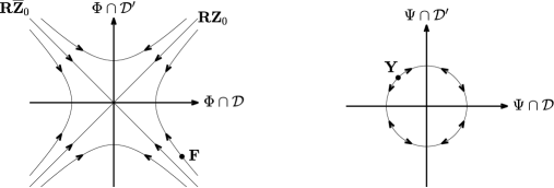
Figure 1: Action of the global automorphism (36) on $\bm{X}_{0}=\bm{F}+\bm{Y}$.

It depends on whether we are in a generic situation, where $\bm{Y}\not=0$ and $\bm{F}$ is neither a real multiple of $\bm{Z}_{0}$ nor of $\overline{\bm{Z}_{0}}$, or in one of the special ones. In the generic case we can rotate $\bm{F}$ to a matrix $f\bm{I}_{2}\in{\mathcal{D}}\cap\bm{\Phi}$ or $if\bm{R}_{\perp}\in{\mathcal{D}}^{\prime}\cap\bm{\Phi}$, depending on whether $|\mathrm{Tr}\,\bm{F}|$ is greater or smaller than $2|\mathfrak{Im}(F_{12})|$, respectively. While we can rotate $\bm{Y}$ to $\psi(y)\in{\mathcal{D}}\cap\bm{\Psi}$ or in $\psi(iy)\in{\mathcal{D}}^{\prime}\cap\bm{\Psi}$, $y>0$, as desired, i.e. according to which space the component $\bm{F}$ can be rotated to. In that case either the physically trivial exact relation $({\mathcal{D}},{\mathcal{D}})$ can be used or an exact relation $({\mathcal{D}},{\mathcal{D}}^{\prime})$ is applicable, unless $\det(\bm{X}_{0})=0$, in which case $\mathrm{Ann}(\mathbb{C}\bm{e}_{2})\subset({\mathcal{D}},{\mathcal{D}})$ exact relation would apply. There are the following special cases

1. $\bm{Y}\not=0$, $\bm{F}\in\mathbb{R}\bm{Z}_{0}$ or $\bm{F}\in\mathbb{R}\overline{\bm{Z}_{0}}$ and $\bm{F}\not=0$. Exact relation $(W,V_{\infty})\sim(\overline{W},\overline{V_{\infty}})$ is applicable.

2. $\bm{Y}\not=0$, $\bm{F}=0$. Exact relation $(\mathbb{C}\bm{I},\mathbb{R}\bm{Y})\sim(\mathbb{C}\bm{I},\mathbb{R}\psi(i))=(\mathbb{C}\bm{I},\Psi)\cap({\mathcal{D}},{\mathcal{D}}^{\prime})$ is applicable.

3. $\bm{Y}=0$, $\bm{F}\not\in\mathbb{R}\bm{Z}_{0}$, $\bm{F}\not\in\mathbb{R}\overline{\bm{Z}_{0}}$. Exact relation $(\mathbb{C}\bm{I},\mathbb{R}\bm{F})$ is applicable. If we are in a strongly coupled case then $(\mathbb{C}\bm{I},\mathbb{R}\bm{F})\sim(\mathbb{C}\bm{I},i\bm{R}_{\perp})=(\mathbb{C}\bm{I},\Psi)\cap({\mathcal{D}},{\mathcal{D}}^{\prime})$, otherwise, $(\mathbb{C}\bm{I},\mathbb{R}\bm{F})\sim(\mathbb{C}\bm{I},\mathbb{R}\bm{I})=(\mathbb{C}\bm{I},\Psi)\cap({\mathcal{D}},{\mathcal{D}})$.

4. $\bm{Y}=0$ and $\bm{F}\in\mathbb{R}\bm{Z}_{0}$ or $\bm{F}\in\mathbb{R}\overline{\bm{Z}_{0}}$ and $\bm{F}\not=0$. Exact relation $(0,\mathbb{R}\bm{Z}_{0})\sim(0,\mathbb{R}\overline{\bm{Z}_{0}})$ is applicable.

Thus, if both components of $\bm{X}_{0}$ are non-zero then there are 4 exact relations between components of $\mathsf{L}^{*}$. What is interesting is that the form of these relations depends very much on specific values of the components. If one of the components of $\bm{X}_{0}$ happens to be 0, then there would be at least 7 exact relations, rising to 9 in a very special case $\bm{X}_{0}=x_{0}\bm{Z}_{0}$ or $\bm{X}_{0}=x_{0}\overline{\bm{Z}_{0}}$, in this very special case all components of $\mathsf{L}^{*}$ will be uniquely determined if the volume fractions of the components are known.

If we write $\mathsf{L}_{j}=\bm{\sigma}_{j}\otimes\bm{I}_{2}+r_{j}\mathsf{T}$. Then the transformation

$$\Psi(\mathsf{L})=(\bm{\sigma}_{1}^{-1/2}\otimes\bm{I}_{2})(\mathsf{L}-r_{1}\mathsf{T})(\bm{\sigma}_{1}^{-1/2}\otimes\bm{I}_{2})$$ (108)

maps $\mathsf{L}_{1}$ to $\mathsf{I}$, while

$$\mathsf{L}^{\prime}=\Psi(\mathsf{L}_{2})=K\left(\bm{\sigma}_{1}^{-1/2}\bm{\sigma}_{2}\bm{\sigma}_{1}^{-1/2}+\frac{r_{2}-r_{1}}{\sqrt{\det{\bm{\sigma}_{1}}}}i\bm{R}_{\perp},0\right).$$

Next we apply transformation $\Psi_{\bm{A},\bm{I}_{2}}$, where

$$\bm{A}=\left[\begin{array}[]{cc}\displaystyle{a_{0}}&\displaystyle{1}\\[4.30554pt] \displaystyle{1}&\displaystyle{a_{0}}\end{array}\right]$$

These transformations have the property that $\Psi(\mathsf{I})=\mathsf{I}$. Then denoting

$$\bm{\sigma}=\bm{\sigma}_{1}^{-1/2}\bm{\sigma}_{2}\bm{\sigma}_{1}^{-1/2},\qquad\rho=\frac{r_{2}-r_{1}}{\sqrt{\det{\bm{\sigma}_{1}}}},$$ (109)

we obtain

$$\Psi_{\bm{A},\bm{I}_{2}}(K(\bm{\sigma}+i\rho\bm{R}_{\perp},0))=K(\bm{L},0),\quad\bm{L}=i\bm{R}_{\perp}(\bm{\sigma}+i(\rho+a_{0})\bm{R}_{\perp})^{-1}(a_{0}\bm{\sigma}+i(a_{0}\rho+1)\bm{R}_{\perp}).$$

Since all the matrices involved in the formula for $\bm{L}$ are $2\times 2$ we have

$$(\bm{\sigma}+i(\rho+a_{0})\bm{R}_{\perp})^{-1}=\frac{\bm{R}_{\perp}^{T}(\bm{\sigma}-i(\rho+a_{0})\bm{R}_{\perp})\bm{R}_{\perp}}{\det\bm{\sigma}-(\rho+a_{0})^{2}}.$$

Thus,

$$\bm{L}=\frac{(1-a_{0}^{2})\bm{\sigma}+i(a_{0}\det\bm{\sigma}-(\rho+a_{0})(a_{0}\rho+1))\bm{R}_{\perp}}{\det\bm{\sigma}-(\rho+a_{0})^{2}}.$$ (110)

Let us now choose $a_{0}$ so that the matrix $\bm{L}$ is real and symmetric. This means that $a_{0}$ must be a root of

$$(a_{0}^{2}+1)\rho=a_{0}(\det\bm{\sigma}-(\rho^{2}+1)).$$ (111)

It is easy to check that the discriminant of the quadratic equation (111) is nonnegative if and only if

$$|r_{1}-r_{2}|\leq\left|\sqrt{\det\bm{\sigma}_{1}}-\sqrt{\det\bm{\sigma}_{2}}\right|.$$ (112)

We will call this case “weakly coupled” because there is a choice of $a_{0}$ (a root of (111)) that eliminates the thermoelectric coupling from both materials. The exceptional cases are $\det\bm{\sigma}=(\rho\pm 1)^{2}$, in which case the inverse in the definition of $\bm{L}$ does not exist. We note that there are several possibilities.

1. We could have mapped $\mathsf{L}_{2}$ to $\mathsf{I}$, instead of $\mathsf{L}_{1}$. That means that instead of a pair of numbers $(\rho,\det\bm{\sigma})$ we will get a pair of numbers

   $$(\rho^{\prime},\det\bm{\sigma}^{\prime})=\left(-\frac{\rho}{\sqrt{\det\bm{\sigma}}},\displaystyle\frac{1}{\det\bm{\sigma}}\right).$$

   It is easy to check that the sign of the discriminant of (111) does not depend on the choice of which $\mathsf{L}_{j}$ gets mapped to $\mathsf{I}$.

2. In each case there are two real roots $a_{0}$. If one root is $a_{0}$, the other root is $1/a_{0}$.

We want $\bm{L}>0$. This means that in each case we must have the inequality

$$\frac{1-a_{0}^{2}}{\det\bm{\sigma}-(\rho+a_{0})^{2}}>0.$$

In the weakly coupled case (111) we have

$$\frac{1-a_{0}^{2}}{\det\bm{\sigma}-(\rho+a_{0})^{2}}=\frac{a_{0}}{\rho+a_{0}}=\frac{a_{0}\rho+1}{\det\bm{\sigma}}.$$

If $a_{1}$ and $a_{2}$ are the two roots of (111), then

$$\frac{a_{1}}{\rho+a_{1}}\cdot\frac{a_{2}}{\rho+a_{2}}=\displaystyle\frac{1}{\det\bm{\sigma}}>0,$$

$$\frac{a_{1}}{\rho+a_{1}}+\frac{a_{2}}{\rho+a_{2}}=\frac{\det\bm{\sigma}-\rho^{2}+1}{\det\bm{\sigma}}.$$

The inequality $\det\bm{\sigma}-\rho^{2}+1>0$ always holds in the weakly coupled case.

In the strongly coupled case, i.e. when inequality (112) is violated, we first apply the transformation

$$\Psi_{0}(\mathsf{L})=(\bm{\sigma}_{1}^{-1/2}\otimes\bm{I}_{2})\mathsf{L}(\bm{\sigma}_{1}^{-1/2}\otimes\bm{I}_{2})$$

which mapps $\bm{L}_{1}$ into $\bm{L}^{\prime}_{1}=\bm{I}_{2}+i\rho_{1}\bm{R}_{\perp}$, and $\bm{L}_{2}$ into $\bm{L}^{\prime}_{2}=\bm{\sigma}+i\rho_{2}\bm{R}_{\perp}$, where

$$\rho_{j}=\frac{r_{j}}{\sqrt{\det{\bm{\sigma}_{1}}}}.$$

In this case we look for a simpler transformation

$$\Psi_{3}(\mathsf{L})=a\mathsf{L}+b\mathsf{T},$$

which maps $\mathsf{L}^{\prime}_{j}$ onto the ER $({\mathcal{D}},{\mathcal{D}}^{\prime})$ if we work in the frame in which $\bm{\sigma}_{11}=\bm{\sigma}_{22}$. The coefficients $a>0$ and $b\in\mathbb{R}$ need to be chosen so that

$$\det(a\bm{I}_{2}+i(a\rho_{1}+b)\bm{R}_{\perp})=\det(a\bm{\sigma}+i(a\rho_{2}+b)\bm{R}_{\perp})=1$$

This means that

$$a^{2}=(a\rho_{1}+b)^{2}+1,\qquad a^{2}\det\bm{\sigma}=(a\rho_{2}+b)^{2}+1.$$

Subtracting the two equations we find

$$b=a\frac{\det\bm{\sigma}-1+\rho_{1}^{2}-\rho_{2}^{2}}{2\rho},$$

where $\rho$ is the same as before. We then find that

$$a^{2}\frac{((\rho+1)^{2}-\det\bm{\sigma})(\det\bm{\sigma}-(\rho-1)^{2})}{4\rho^{2}}=1.$$

We note that since $|\rho_{1}|<1$ and $|\rho_{2}|<\sqrt{\det\bm{\sigma}}$, then

$$|\rho|=|\rho_{2}-\rho_{1}|\leq|\rho_{2}|+|\rho_{1}|<\sqrt{\det\bm{\sigma}}+1.$$

This is equivalent to

$$|r_{2}-r_{1}|<\sqrt{\det\bm{\sigma}_{1}}+\sqrt{\det\bm{\sigma}_{2}}.$$

Using our original parameters we can write

$$a^{2}=\frac{4\Delta r^{2}\det\bm{\sigma}_{1}}{(\Delta r^{2}-(\sqrt{\det\bm{\sigma}_{1}}-\sqrt{\det\bm{\sigma}_{2}})^{2})((\sqrt{\det\bm{\sigma}_{1}}+\sqrt{\det\bm{\sigma}_{2}})^{2}-\Delta r^{2})},\qquad\Delta r=r_{2}-r_{1}$$

This shows that in the strongly coupled regime we can always choose $a>0$. We will therefore write

$$a=2a_{0}\sqrt{\det\bm{\sigma}_{1}},\quad a_{0}=\frac{|\Delta r|}{\sqrt{(\Delta r^{2}-(\sqrt{\det\bm{\sigma}_{1}}-\sqrt{\det\bm{\sigma}_{2}})^{2})((\sqrt{\det\bm{\sigma}_{1}}+\sqrt{\det\bm{\sigma}_{2}})^{2}-\Delta r^{2})}}$$

$$b=a_{0}\frac{\det\bm{\sigma}_{2}+r_{1}^{2}-r_{2}^{2}}{r_{2}-r_{1}}.$$

Let us find the conditions for each case, including special cases explicitly in terms of $\bm{\sigma}_{j}$, $r_{j}$, $j=1,2$. We compute

$$\bm{X}_{0}=2\left(\bm{\sigma}_{1}^{-1/2}\bm{\sigma}_{2}\bm{\sigma}_{1}^{-1/2}+\bm{I}_{2}+\frac{r_{2}-r_{1}}{\sqrt{\det{\bm{\sigma}_{1}}}}i\bm{R}_{\perp}\right)^{-1}-\bm{I}_{2}.$$

It fairly easy to show that $\bm{Y}\not=0$ if and only if $\bm{\sigma}_{1}$ and $\bm{\sigma}_{1}$ are not scalar multiples of one another. it is also easy to show that $\bm{F}=0$ if and only if $r_{1}=r_{2}$ and $\det\bm{\sigma}_{1}=\det\bm{\sigma}_{2}$. In order to split $\bm{X}_{0}$ into the $\bm{\Phi}$ and $\bm{\Psi}$ parts we can use the formula

$$(\varphi(\alpha)+\psi(a)+ir\bm{R}_{\perp})^{-1}=\frac{\varphi(\alpha)-\psi(a)-ir\bm{R}_{\perp}}{\alpha^{2}-|a|^{2}-r^{2}}.$$

So, if $\bm{F}=\varphi(\alpha)+ir\bm{R}_{\perp}$ and $\bm{Y}=\psi(a)$, then we have the equation

$$\bm{\sigma}_{1}^{-1/2}\bm{\sigma}_{2}\bm{\sigma}_{1}^{-1/2}+\bm{I}_{2}+\frac{r_{2}-r_{1}}{\sqrt{\det{\bm{\sigma}_{1}}}}i\bm{R}_{\perp}=2\frac{\varphi(\alpha+1)-\psi(a)-ir\bm{R}_{\perp}}{(\alpha+1)^{2}-|a|^{2}-r^{2}}.$$

Hence we have the following system

$$\begin{cases}\frac{r_{2}-r_{1}}{\sqrt{\det{\bm{\sigma}_{1}}}}=-\frac{2r}{(\alpha+1)^{2}-|a|^{2}-r^{2}},\\ \mathrm{Tr}\,(\bm{\sigma}_{2}\bm{\sigma}_{1}^{-1})+2=\frac{4(\alpha+1)}{(\alpha+1)^{2}-|a|^{2}-r^{2}},\\ \frac{\det\bm{\sigma}_{2}}{\det\bm{\sigma}_{1}}=\det\left(2\frac{\varphi(\alpha+1)-\psi(a)}{(\alpha+1)^{2}-|a|^{2}-r^{2}}-\varphi(1)\right).\end{cases}$$

The condition that $\bm{F}\in\mathbb{R}\bm{Z}_{0}$ or $\bm{F}\in\mathbb{R}\overline{\bm{Z}_{0}}$ is equivalent to $r^{2}=\alpha^{2}$.

$$\begin{cases}|a|^{2}=\frac{\mathrm{Tr}\,(\bm{\sigma}_{1}\mathrm{cof}(\bm{\sigma}_{2}))^{2}-4\det(\bm{\sigma}_{1}\bm{\sigma}_{2})}{(\det(\bm{\sigma}_{1}+\bm{\sigma}_{2})-(r_{1}-r_{2})^{2})^{2}},\\ r^{2}=\frac{4(r_{1}-r_{2})^{2}\det(\bm{\sigma}_{1})}{(\det(\bm{\sigma}_{1}+\bm{\sigma}_{2})-(r_{1}-r_{2})^{2})^{2}},\\ \alpha=\frac{(r_{1}-r_{2})^{2}+\det(\bm{\sigma}_{1})-\det(\bm{\sigma}_{2})}{\det(\bm{\sigma}_{1}+\bm{\sigma}_{2})-(r_{1}-r_{2})^{2}}\end{cases}$$

The condition that $\bm{F}\in\mathbb{R}\bm{Z}_{0}$ or $\bm{F}\in\mathbb{R}\overline{\bm{Z}_{0}}$ is equivalent to

$$|r_{1}-r_{2}|=\left|\sqrt{\det\bm{\sigma}_{1}}-\sqrt{\det\bm{\sigma}_{2}}\right|.$$ (113)

The composite made with the pair of isotropic materials $\mathsf{L}_{j}$ will be called weakly thermoelectrically heterogenerous if

$$|r_{1}-r_{2}|<\left|\sqrt{\det\bm{\sigma}_{1}}-\sqrt{\det\bm{\sigma}_{2}}\right|,$$ (114)

and strongly coupled otherwise. (We note that requirement of positive definteness of $\mathsf{L}_{j}$ implies that $r_{j}^{2}<\det\bm{\sigma}_{j}$.) The thermoelectric interactions in a weakly thermoelectrically heterogenerous composite can be decoupled. Such a decoupling is impossible in a strongly thermoelectrically heterogenerous composite. Here is the summary.

1. $\bm{\sigma}_{1}\not=\theta\bm{\sigma}_{2}$ (generic case)

   1. $|r_{1}-r_{2}|<\left|\sqrt{\det\bm{\sigma}_{1}}-\sqrt{\det\bm{\sigma}_{2}}\right|$ (weakly coupled case)

      1. $|r_{1}-r_{2}|^{2}\not=\det(\bm{\sigma}_{1}-\bm{\sigma}_{2})$: ER $({\mathcal{D}},{\mathcal{D}})$. This implies that the 10 components of $\mathsf{L}^{*}$ depend only on 6 microstructure-dependent parameters. Moreover, the link $({\mathcal{D}},{\mathcal{D}})/{\rm Ann}(\mathbb{C}\bm{e}_{2})\cong{\rm Ann}(\mathbb{C}\bm{e}_{2})$ that relates $\mathsf{L}^{*}$ to the effective tensor of a 2D conducting composite applies.

      2. $|r_{1}-r_{2}|^{2}=\det(\bm{\sigma}_{1}-\bm{\sigma}_{2})$: ER Ann$(\mathbb{C}\bm{e}_{2})$. This implies that the 10 components of $\mathsf{L}^{*}$ depend only on 3 microstructure-dependent parameters. Moreover, they can be expressed in terms of the effective tensor of a 2D conducting composite.

   2. $|r_{1}-r_{2}|>\left|\sqrt{\det\bm{\sigma}_{1}}-\sqrt{\det\bm{\sigma}_{2}}\right|$: ER $({\mathcal{D}},{\mathcal{D}}^{\prime})$ (strongly coupled case) This implies that the 10 components of $\mathsf{L}^{*}$ depend only on 6 microstructure-dependent parameters.

   3. $|r_{1}-r_{2}|=\left|\sqrt{\det\bm{\sigma}_{1}}-\sqrt{\det\bm{\sigma}_{2}}\right|$ (borderline strongly coupled case)

      1. $r_{1}\not=r_{2}$: ER $(W,V_{\infty})$. This implies that the 10 components of $\mathsf{L}^{*}$ depend only on 6 microstructure-dependent parameters. Moreover, the link $(W,V_{\infty})/{\rm Ann}(\mathbb{C}\overline{\bm{z}_{0}})\cong(\mathbb{C}\bm{I},\mathbb{R}\psi(i))$ is applicable. This means that there is a link between this case and the $r_{1}=r_{2}$ case, since ERs $(\mathbb{C}\bm{I},\mathbb{R}\psi(i))$ and $(\mathbb{C}\bm{I},\mathbb{R}\psi(1))$ are isomorphic.

      2. $r_{1}=r_{2}$: ER $(\mathbb{C}\bm{I},\mathbb{R}\psi(1))$. This implies that the 10 components of $\mathsf{L}^{*}$ depend only on 3 microstructure-dependent parameters, expressible in terms of 2D conductivity.

2. $\bm{\sigma}_{1}=\theta_{1}\bm{\sigma}$, $\bm{\sigma}_{2}=\theta_{2}\bm{\sigma}$ (special nongeneric case)

   1. $|r_{1}-r_{2}|<|\theta_{1}-\theta_{2}|\sqrt{\det\bm{\sigma}}$: ER $(\mathbb{C}\bm{I},\mathbb{R}\bm{I})$. This implies that the 10 components of $\mathsf{L}^{*}$ depend only on 3 microstructure-dependent parameters, which are expressible in terms of the effective tensor of a 2D conducting composite.

   2. $|r_{1}-r_{2}|>|\theta_{1}-\theta_{2}|\sqrt{\det\bm{\sigma}}$: ER $(\mathbb{C}\bm{I},i\bm{R}_{\perp})$. This implies that the 10 components of $\mathsf{L}^{*}$ depend only on 3 microstructure-dependent parameters.

   3. $|r_{1}-r_{2}|=|\theta_{1}-\theta_{2}|\sqrt{\det\bm{\sigma}}$: ER $(0,\mathbb{R}\bm{Z}_{0})$. This implies $\mathsf{L}^{*}$ is completely determined, regardless of microstructure, if the volue fractions are known.

An example is a binary composite made with isotropic thermoelectric materials in which the Seebeck coefficient $\bm{S}$ is a scalar. In this case we have $r_{1}=r_{2}=0$. Let $\Sigma^{*}(h)$ be the effective tensor of an isotropic conducting composite made with two isotropic materials, whose conductivities are 1 and $h$. Then $\bm{\Sigma}^{*}$ can be applied to symmetric matrices according to the rule

$$\Sigma^{*}(\bm{S})=\bm{R}\left[\begin{array}[]{cc}\displaystyle{\Sigma^{*}(s_{1})}&\displaystyle{0}\\[4.30554pt] \displaystyle{0}&\displaystyle{\Sigma^{*}(s_{2})}\end{array}\right]\bm{R}^{T},\qquad\bm{S}=\bm{R}\left[\begin{array}[]{cc}\displaystyle{s_{1}}&\displaystyle{0}\\[4.30554pt] \displaystyle{0}&\displaystyle{s_{2}}\end{array}\right]\bm{R}^{T}.$$

Then the effective thermoelectric tensor of such a composite will be isotropic and also have scalar Seebeck coefficient $r^{*}=0$ and

$$\mathsf{L}^{*}=\bm{\sigma}^{*}\otimes\bm{I}_{2},\qquad\bm{\sigma}^{*}=\bm{\sigma}_{1}^{1/2}\Sigma^{*}(\bm{\sigma}_{1}^{-1/2}\bm{\sigma}_{2}\bm{\sigma}_{1}^{-1/2})\bm{\sigma}_{1}^{1/2}.$$

28.2 Results

In many cases the results will be formulated in terms of the microstructure-dependent function $\bm{\Sigma}(h)$, representing the effictive conductivity of a two-phase composite with isotropic constituent conductivities $\bm{I}_{2}$ and $h\bm{I}_{2}$, replacing materials $\mathsf{L}_{1}$, $\mathsf{L}_{2}$ in the original composite. Another convenient notation will be matrices $\bm{S}_{1}$ and $\bm{S}_{2}$ definied by

$$\bm{S}_{1}=\frac{\bm{\sigma}_{2}-\lambda_{1}\bm{\sigma}_{1}}{\lambda_{2}-\lambda_{1}},\qquad\bm{S}_{2}=\frac{\bm{\sigma}_{2}-\lambda_{2}\bm{\sigma}_{1}}{\lambda_{1}-\lambda_{2}},$$

where $\lambda_{1}$ and $\lambda_{2}$ are the two roots of the quadratic equation $\det(\bm{\sigma}_{2}-\lambda\bm{\sigma}_{1})=0$. The ordering of the roots is unimportant. This notation will not be used when $\bm{\sigma}_{1}$ and $\bm{\sigma}_{2}$ are scalar multiples of one another, since in this case $\lambda_{1}=\lambda_{2}$ and the matrices $S_{j}$ are undefined.

$\bullet$ (2(c)) $\bm{\sigma}_{1}=\theta_{1}\bm{\sigma}_{0}$, $\bm{\sigma}_{2}=\theta_{2}\bm{\sigma}_{0}$, $|r_{1}-r_{2}|=|\theta_{1}-\theta_{2}|\sqrt{\det\bm{\sigma}_{0}}$. We apply the global automorphism

$$\Psi(\mathsf{L})=\displaystyle\frac{1}{\theta_{1}}(\bm{\sigma}_{0}^{-1/2}\otimes\bm{I}_{2})(\mathsf{L}-r_{1}\mathsf{T})(\bm{\sigma}_{0}^{-1/2}\otimes\bm{I}_{2}),$$

which maps $\mathsf{L}_{1}$ into $\mathsf{I}$ and $\mathsf{L}_{2}$ into

$$\mathsf{L}_{0}=\left[\begin{array}[]{cc}\displaystyle{\frac{\theta_{2}}{\theta_{1}}\bm{I}_{2}}&\displaystyle{-\frac{r_{2}-r_{1}}{\theta_{1}\sqrt{\det\bm{\sigma}_{0}}}\bm{R}_{\perp}}\\[4.30554pt] \displaystyle{\frac{r_{2}-r_{1}}{\theta_{1}\sqrt{\det\bm{\sigma}_{0}}}\bm{R}_{\perp}}&\displaystyle{\frac{\theta_{2}}{\theta_{1}}\bm{I}_{2}}\end{array}\right],$$

corresponding to the ER $(0,\mathbb{R}\bm{Z}_{0})$ or $(0,\mathbb{R}\overline{\bm{Z}_{0}})$. We choose indexing in such a way that $\theta_{2}\geq\theta_{1}$, so that $\mathsf{L}_{0}>0$. If we denote

$$\lambda=\frac{\theta_{2}}{\theta_{1}}\geq 1,$$

then either

$$\frac{r_{2}-r_{1}}{\theta_{1}\sqrt{\det\bm{\sigma}_{0}}}=\lambda-1,\text{ or }\frac{r_{2}-r_{1}}{\theta_{1}\sqrt{\det\bm{\sigma}_{0}}}=-(\lambda-1),$$

depending on whether $r_{1}-r_{2}=(\theta_{1}-\theta_{2})\sqrt{\det\bm{\sigma}_{0}}$ or $r_{1}-r_{2}=-(\theta_{1}-\theta_{2})\sqrt{\det\bm{\sigma}_{0}}$, respectively. In either case the effective tensor of a composite made with $\mathsf{I}$ and $\mathsf{L}_{0}$ will have the form

$$\mathsf{L}^{*}_{0}=\left[\begin{array}[]{cc}\displaystyle{\lambda^{*}\bm{I}_{2}}&\displaystyle{\mp(\lambda^{*}-1)\bm{R}_{\perp}}\\[4.30554pt] \displaystyle{\pm(\lambda^{*}-1)\bm{R}_{\perp}}&\displaystyle{\lambda^{*}\bm{I}_{2}}\end{array}\right],\qquad\displaystyle\frac{1}{\lambda^{*}}=\langle\lambda(x)^{-1}\rangle=f_{1}+\frac{f_{2}}{\lambda}.$$

Applying $\Psi^{-1}$ transformation we obtain the formula for $\mathsf{L}^{*}=K(\bm{\sigma}^{*}+ir^{*}\bm{R}_{\perp},0)$:

$$\bm{\sigma}^{*}=(f_{1}\bm{\sigma}_{1}^{-1}+f_{2}\bm{\sigma}_{2}^{-1})^{-1},\qquad r^{*}=r_{1}+\frac{(r_{2}-r_{1})f_{2}\theta_{1}}{f_{1}\theta_{2}+f_{2}\theta_{1}}=\frac{r_{1}f_{1}\theta_{1}^{-1}+r_{2}f_{2}\theta_{2}^{-1}}{f_{1}\theta_{1}^{-1}+f_{2}\theta_{2}^{-1}}.$$

In other words,

$$\bm{\sigma}^{*}=\langle\bm{\sigma}(\bm{x})^{-1}\rangle^{-1},\qquad r^{*}=\frac{\langle r(x)\theta(x)^{-1}\rangle}{\langle\theta(x)^{-1}\rangle}.$$ (115)

In every case we will work in the frame in which $\bm{\sigma}_{1}^{-1/2}\bm{\sigma}_{2}\bm{\sigma}_{1}^{-1/2}$ is diagonal! This is not a physical frame. Rather it is a mathematical one, where two different linear combinations of the original curl-free and divergence-free fields are chosen as a pair of intensity and flux fields.

$\bullet$ (1(c)ii) $\bm{L}_{1}=\bm{\sigma}_{1}+ir_{0}\bm{R}_{\perp}$, $\bm{L}_{2}=\bm{\sigma}_{2}+ir_{0}\bm{R}_{\perp}$, moreover, $\det\bm{\sigma}_{1}=\det\bm{\sigma}_{2}$. The global link (108) maps $\bm{L}_{1}$ to $\bm{I}_{2}$ and $\bm{L}_{2}$ to $\bm{\sigma}=\bm{\sigma}_{1}^{-1/2}\bm{\sigma}_{2}\bm{\sigma}_{1}^{-1/2}$, which is always assumed to be diagonal. Since in this case we have $\det\bm{\sigma}=1$ we can write

$$\bm{\sigma}=\left[\begin{array}[]{cc}\displaystyle{\lambda}&\displaystyle{0}\\[4.30554pt] \displaystyle{0}&\displaystyle{\lambda^{-1}}\end{array}\right],$$

where the eigenvalues $\lambda$ and $1/\lambda$ solve the quadratic equation

$$\det(\bm{\sigma}_{2}-\lambda\bm{\sigma}_{1})=0.$$ (116)

The effective tensor of the resulting composite is

$$\mathsf{L}_{0}^{*}=\left[\begin{array}[]{cc}\displaystyle{\bm{\sigma}^{*}}&\displaystyle{0}\\[4.30554pt] \displaystyle{0}&\displaystyle{\frac{\bm{\sigma}^{*}}{\det\bm{\sigma}^{*}}}\end{array}\right]=\left[\begin{array}[]{cc}\displaystyle{1}&\displaystyle{0}\\[4.30554pt] \displaystyle{0}&\displaystyle{\displaystyle\frac{1}{\det\bm{\sigma}^{*}}}\end{array}\right]\otimes\bm{\sigma}^{*},\qquad\bm{\sigma}^{*}=\bm{\Sigma}(\lambda).$$

where $\bm{\sigma}^{*}$ is the effective conductivity of the composite made with 2 isotropic materials of conductivities 1 and $\lambda$ and the same microstructure as the original composite. We conclude that

$$\mathsf{L}^{*}=\bm{\sigma}_{1}^{1/2}\left[\begin{array}[]{cc}\displaystyle{1}&\displaystyle{0}\\[4.30554pt] \displaystyle{0}&\displaystyle{\displaystyle\frac{1}{\det\bm{\sigma}^{*}}}\end{array}\right]\bm{\sigma}_{1}^{1/2}\otimes\bm{\sigma}^{*}+r_{0}\mathsf{T},$$ (117)

where we have used the the form in which terms on both sides of the $\otimes$ sign are invariant with respect to the $\lambda\mapsto\lambda^{-1}$ permutation. We can express the answer without using $\bm{\sigma}_{1}^{1/2}$ by observing that

$$\bm{\sigma}_{1}^{1/2}\bm{I}_{2}\bm{\sigma}_{1}^{1/2}=\bm{\sigma}_{1},\qquad\bm{\sigma}_{1}^{1/2}\bm{\sigma}\bm{\sigma}_{1}^{1/2}=\bm{\sigma}_{2}.$$

In the frame in which $\bm{\sigma}$ is diagonal we obtain

$$\mathsf{L}^{*}=r_{0}\mathsf{T}+((\det\bm{\sigma}^{*}-\lambda^{2})\bm{\sigma}_{1}+\lambda(1-\det\bm{\sigma}^{*})\bm{\sigma}_{2})\otimes\frac{\bm{\sigma}^{*}}{(1-\lambda^{2})\det\bm{\sigma}^{*}},$$

where $\lambda>0$ solves (116) and $\bm{\sigma}^{*}=\Sigma_{\rm 2Dcond}(1,\lambda)$, and the result is independent of the choice of the root in (116). We note that in the notation $\bm{A}\otimes\bm{B}$, the frame of the operator $\bm{B}$ is the physical one, while the frame of $\bm{A}$ is mathematical. In the formula for $\mathsf{L}^{*}$ above the first factor of the tensor product would look the same in the original frame, since the tensors $\bm{\sigma}_{j}$ are transforming together with the mathematical frame. Using our notation $\bm{S}_{1}$ and $\bm{S}_{2}$ are can write the final answer as

$$\mathsf{L}^{*}=r_{0}\mathsf{T}+\left(\frac{\bm{S}_{1}}{\det\bm{\sigma}^{*}}+\bm{S}_{2}\right)\otimes\bm{\sigma}^{*}.$$

$\bullet$ (1(a)ii) $|r_{1}-r_{2}|^{2}=\det(\bm{\sigma}_{1}-\bm{\sigma}_{2})$. In this case the quadratic equation (111) has two solutions $(\lambda_{j}-1)/\rho$, $j=1,2$, where the eigenvalues $\lambda_{1}$ and $\lambda_{2}$ of $\bm{\sigma}$ solve (116). If we choose $a_{0}=(\lambda_{1}-1)/\rho$, then

$$\bm{S}=\left[\begin{array}[]{cc}\displaystyle{\frac{\lambda_{1}}{\lambda_{2}}}&\displaystyle{0}\\[4.30554pt] \displaystyle{0}&\displaystyle{1}\end{array}\right],\qquad\mathsf{L}_{0}^{*}=\left[\begin{array}[]{cc}\displaystyle{\bm{\sigma}^{*}}&\displaystyle{0}\\[4.30554pt] \displaystyle{0}&\displaystyle{\bm{I}_{2}}\end{array}\right],\qquad\bm{\sigma}^{*}=\bm{\Sigma}\left(\frac{\lambda_{1}}{\lambda_{2}}\right).$$ (118)

Inverting our global link that mappled $\mathsf{L}_{1}$ to $\bm{I}_{2}\otimes\bm{I}_{2}$ and $\mathsf{L}_{2}$ to $\bm{S}\otimes\bm{I}_{2}$ we obtain

$$\mathsf{L}^{*}=r_{1}\mathsf{T}+(\bm{\sigma}_{1}^{1/2}\otimes\bm{I}_{2})(\mathsf{T}-a_{0}\mathsf{L}_{0}^{*})(\mathsf{L}_{0}^{*}-a_{0}\mathsf{T})^{-1}\mathsf{T}(\bm{\sigma}_{1}^{1/2}\otimes\bm{I}_{2}).$$

Observe that

$$\mathsf{P}^{*}=(\mathsf{T}-a_{0}\mathsf{L}_{0}^{*})(\mathsf{L}_{0}^{*}-a_{0}\mathsf{T})^{-1}\mathsf{T}=(1-a_{0}^{2})\mathsf{T}(\mathsf{L}_{0}^{*}-a_{0}\mathsf{T})^{-1}\mathsf{T}-a_{0}\mathsf{T}.$$

We then compute (verified by Maple)

$$\mathsf{P}^{*}_{0}=(1-a_{0}^{2})\mathsf{T}(\mathsf{L}_{0}^{*}-a_{0}\mathsf{T})^{-1}\mathsf{T}=\frac{1-a_{0}^{2}}{\det(\bm{\sigma}^{*}-a_{0}^{2})}\left[\begin{array}[]{cc}\displaystyle{\det\bm{\sigma}^{*}-a_{0}^{2}\bm{\sigma}^{*}}&\displaystyle{a_{0}\bm{R}_{\perp}^{T}(\bm{\sigma}^{*}-a_{0}^{2})}\\[4.30554pt] \displaystyle{a_{0}(\bm{\sigma}^{*}-a_{0}^{2})\bm{R}_{\perp}}&\displaystyle{\bm{\sigma}^{*}-a_{0}^{2}}\end{array}\right].$$

Thus,

$$\mathsf{L}^{*}=(r_{1}-a_{0}\sqrt{\det\bm{\sigma}_{1}})\mathsf{T}+(\bm{\sigma}_{1}^{1/2}\otimes\bm{I}_{2})\mathsf{P}^{*}_{0}(\bm{\sigma}_{1}^{1/2}\otimes\bm{I}_{2}).$$ (119)

In order to write $\mathsf{L}^{*}$ without the explicit reference to $\bm{\sigma}_{1}^{1/2}$ we write $\mathsf{P}_{0}^{*}$ as a sum of tensor products. In order to accomplish this we first write $\bm{\sigma}^{*}=\phi(x^{*})+\psi(y^{*})$ and then observe that

$$\bm{R}_{\perp}^{T}\psi(y^{*})=-\psi(iy^{*})=\psi(y^{*})\bm{R}_{\perp}.$$

Thus, we get

$$\mathsf{P}^{*}_{0}=\frac{1-a_{0}^{2}}{\det(\bm{\sigma}^{*}-a_{0}^{2})}\left(\left[\begin{array}[]{cc}\displaystyle{\det\bm{\sigma}^{*}}&\displaystyle{0}\\[4.30554pt] \displaystyle{0}&\displaystyle{-a_{0}^{2}}\end{array}\right]\otimes\bm{I}_{2}+\left[\begin{array}[]{cc}\displaystyle{-a_{0}^{2}}&\displaystyle{0}\\[4.30554pt] \displaystyle{0}&\displaystyle{1}\end{array}\right]\otimes\bm{\sigma}^{*}+a_{0}(x^{*}-a_{0}^{2})\mathsf{T}-a_{0}\psi(i)\otimes\psi(iy^{*})\right)$$

We will then be able to compute $\mathsf{L}^{*}$ in the covariant form, if we can express $\bm{\sigma}_{1}^{1/2}\psi(i)\bm{\sigma}_{1}^{1/2}$, in the covariant form. To do this we first write $\psi(i)=\phi(i)\psi(1)$, and then

$$\bm{\sigma}_{1}^{1/2}\psi(i)\bm{\sigma}_{1}^{1/2}=\bm{\sigma}_{1}^{1/2}\phi(i)\bm{\sigma}_{1}^{1/2}\bm{\sigma}_{1}^{-1}\bm{\sigma}_{1}^{1/2}\psi(1)\bm{\sigma}_{1}^{1/2}=\sqrt{\det\bm{\sigma}_{1}}\bm{R}_{\perp}\bm{\sigma}_{1}^{-1}(\bm{\sigma}_{1}^{1/2}\psi(1)\bm{\sigma}_{1}^{1/2}).$$

Thus, we compute

$$\bm{\sigma}_{1}^{1/2}\psi(1)\bm{\sigma}_{1}^{1/2}=\frac{(\lambda_{1}+\lambda_{2})\bm{\sigma}_{1}-2\bm{\sigma}_{2}}{\lambda_{2}-\lambda_{1}}=\bm{S}_{2}-\bm{S}_{1}.$$

Therefore,

$$\bm{\sigma}_{1}^{1/2}\psi(i)\bm{\sigma}_{1}^{1/2}=\sqrt{\det\bm{\sigma}_{1}}\bm{R}_{\perp}\bm{\sigma}_{1}^{-1}(\bm{S}_{2}-\bm{S}_{1}),$$

which is now in a frame-covariant form. Putting everything together we obtain

$$\mathsf{L}^{*}=\left(r_{1}+a_{0}\left(\frac{(1-a_{0}^{2})(x^{*}-a_{0}^{2})}{\det(\bm{\sigma}^{*}-a_{0}^{2})}-1\right)\sqrt{\det\bm{\sigma}_{1}}\right)\mathsf{T}+\frac{1-a_{0}^{2}}{\det(\bm{\sigma}^{*}-a_{0}^{2})}\times\\ \{\bm{S}_{1}\otimes(\bm{\sigma}^{*}-a_{0}^{2})+\bm{S}_{2}\otimes(\det\bm{\sigma}^{*}-a_{0}^{2}\bm{\sigma}^{*})+a_{0}\sqrt{\det\bm{\sigma}_{1}}\mathsf{T}[\bm{\sigma}_{1}^{-1}(\bm{S}_{1}-\bm{S}_{2})\otimes(\bm{\sigma}^{*}-x^{*})]\}$$ (120)

This expression is invariant with respect to the choice of $\lambda_{1}$ and $\lambda_{2}$. This means that if we interchange $\lambda_{1}$ and $\lambda_{2}$, $\bm{S}_{1}$ and $\bm{S}_{2}$, repalce $a_{0}$ with $1/a_{0}$, and $\bm{\sigma}^{*}$ with $\bm{\sigma}^{*}/\det\bm{\sigma}^{*}$, the value of $\mathsf{L}^{*}$ will not change.

We also want to see if there is a symmetry wrt to material index interchange “1”$\mapsto$”2” (the result should not depend on naming conventions). Hence we need to make the following replacements:

$$\det\bm{\sigma}_{1}\mapsto\lambda_{1}\lambda_{2}\det\bm{\sigma}_{1},\ a_{0}\mapsto a_{0}\sqrt{\frac{\lambda_{2}}{\lambda_{1}}},\ \bm{\sigma}^{*}\mapsto\frac{\lambda_{2}}{\lambda_{1}}\bm{\sigma}^{*},\ \lambda_{j}\mapsto\displaystyle\frac{1}{\lambda_{j}},\ \bm{S}_{j}\mapsto\lambda_{1}\lambda_{2}\frac{\bm{S}_{j}}{\lambda_{j}}.$$

We can verify that the second term is invariant. This is due to the observation that, since

$$a_{0}=\frac{\lambda_{1}-1}{\rho}=\frac{\rho}{\lambda_{2}-1},$$

we can also write

$$a_{0}^{2}=\frac{\lambda_{1}-1}{\lambda_{2}-1}\quad\Rightarrow\quad 1-a_{0}^{2}=\frac{\lambda_{2}-\lambda_{1}}{\lambda_{2}-1}.$$

This shows that under the index-interchange we also have $1-a_{0}^{2}\mapsto\displaystyle\frac{1}{\lambda_{1}}(1-a_{0}^{2})$. The first term was also verified to be invariant, since we can write

$$r_{1}=\frac{r_{1}+r_{2}}{2}-\displaystyle\frac{1}{2}\rho\sqrt{\det\bm{\sigma}_{1}}=\frac{r_{1}+r_{2}}{2}-\displaystyle\frac{1}{2}a_{0}(\lambda_{2}-1)\sqrt{\det\bm{\sigma}_{1}}.$$

If $\bm{\sigma}^{*}=x^{*}\bm{I}_{2}$, the result simplifies:

$$\mathsf{L}^{*}=\left(r_{1}+\frac{(1-x^{*})a_{0}}{x^{*}-a_{0}^{2}}\sqrt{\det\bm{\sigma}_{1}}\right)\mathsf{T}+\frac{1-a_{0}^{2}}{x^{*}-a_{0}^{2}}(\bm{S}_{1}+x^{*}\bm{S}_{2})\otimes\bm{I}_{2}.$$ (121)

In order to verify (120) with Maple we can parametrize this case by $\bm{s}=\bm{\sigma}_{1}^{1/2}$, $\lambda_{1}$, $\rho$, $r_{1}$, so that

$$\bm{\sigma}_{1}=\bm{s}^{2},\quad r_{2}=\rho\det\bm{s}+r_{1},\quad\lambda_{2}=\frac{\rho^{2}}{\lambda_{1}-1}+1,\quad\bm{\sigma}_{2}=\bm{s}\left[\begin{array}[]{cc}\displaystyle{\lambda_{1}}&\displaystyle{0}\\[4.30554pt] \displaystyle{0}&\displaystyle{\lambda_{2}}\end{array}\right]\bm{s},\quad a_{0}=\frac{\lambda_{1}-1}{\rho}.$$

Substituting these and $\mathsf{L}_{0}^{*}$ given by (118) into (119) we obtain (120), as verified by Maple. Formula (121) has also been verified.

Finally we point out that the case $a_{0}=\infty$ corresponding to $r_{1}=r_{2}=r_{0}$ and $\det(\bm{\sigma}_{1}-\bm{\sigma}_{2})=0$ is also included by taking a limit as $a_{0}\to\infty$ in (120):

$$\mathsf{L}^{*}=r_{0}\mathsf{T}+\bm{S}_{1}\otimes\bm{I}_{2}+\bm{S}_{2}\otimes\bm{\Sigma}^{*}(\lambda_{1}),\quad\lambda_{1}\not=1=\lambda_{2}.$$

$\bullet$ (1(c)i): $|r_{1}-r_{2}|=\left|\sqrt{\det\bm{\sigma}_{1}}-\sqrt{\det\bm{\sigma}_{2}}\right|$. The relevant ER is $(W,V_{0})$, described as

$$\left\{\left[\begin{array}[]{cc}\displaystyle{\bm{L}}&\displaystyle{\pm(\bm{L}\bm{M}-\bm{R}_{\perp})}\\[4.30554pt] \displaystyle{\pm(\bm{M}^{T}\bm{L}+\bm{R}_{\perp})}&\displaystyle{\bm{M}^{T}\bm{L}\bm{M}}\end{array}\right]:\mathrm{Tr}\,\bm{M}=0,\ \bm{L}>0,\ \bm{L}+2\bm{R}_{\perp}\bm{M}\det\bm{L}<0\right\}.$$ (122)

The relevant link is as follows. $\bm{M}^{*}=\bm{R}_{\perp}\bm{\sigma}^{*}$, where $\bm{\sigma}^{*}$ is the 2D effective condictivity tensor of the composite with local conductivity $\bm{c}(\bm{x})=-\bm{R}_{\perp}\bm{M}(\bm{x})$, which is symmetric and positive definite for $\bm{M}(\bm{x})$ satisfying the constraints in (122).

Any isotropic tensor $\mathsf{L}$ in this ER must have the form

$$\mathsf{L}=\left[\begin{array}[]{cc}\displaystyle{\lambda_{1}\bm{I}_{2}}&\displaystyle{\pm(\sqrt{\lambda_{1}\lambda_{2}}-1)\bm{R}_{\perp}}\\[4.30554pt] \displaystyle{\mp(\sqrt{\lambda_{1}\lambda_{2}}-1)\bm{R}_{\perp}}&\displaystyle{\lambda_{2}\bm{I}_{2}}\end{array}\right],\qquad\lambda_{1}>0,\ \lambda_{1}\lambda_{2}>\displaystyle\frac{1}{4},$$

corresponding to $\bm{M}=\sqrt{\lambda_{2}/\lambda_{1}}\bm{R}_{\perp}$. Thus,

$$\mathsf{L}_{0}^{*}=\left[\begin{array}[]{cc}\displaystyle{\bm{L}^{*}}&\displaystyle{\pm\bm{R}_{\perp}\mathrm{cof}(\bm{L}^{*})\bm{\sigma}^{*}}\\[4.30554pt] \displaystyle{\pm\bm{\sigma}^{*}\mathrm{cof}(\bm{L}^{*})\bm{R}_{\perp}^{T}}&\displaystyle{\bm{\sigma}^{*}\mathrm{cof}(\bm{L}^{*})\bm{\sigma}^{*}}\end{array}\right]\pm\mathsf{T},$$ (123)

where $\bm{\sigma}^{*}=\bm{\Sigma}^{*}(\sqrt{\lambda_{2}/\lambda_{1}})$, where $\lambda_{1,2}$ are the two roots of (116), and $\bm{L}^{*}$ is microstructure-dependent tensor that depends on material moduli only through $\lambda_{1}$ and $\lambda_{2}$. It is not expressible in terms of the effective conductivity. To compute $\mathsf{L}^{*}$ we take $\Psi^{-1}$ and obtain as in the case 1(a)ii

$$\mathsf{L}^{*}=\bm{S}_{1}\otimes\bm{\sigma}^{*}\mathrm{cof}(\bm{L}^{*})\bm{\sigma}^{*}+\bm{S}_{2}\otimes\bm{L}^{*}+\alpha\mathsf{T}\left[\bm{\sigma}_{1}^{-1}(\bm{S}_{1}-\bm{S}_{2})\otimes\bm{A}^{*}\right]+\beta\mathsf{T},$$

where

$$\bm{A}^{*}=\mathrm{cof}(\bm{L}^{*})\bm{\sigma}^{*}-a^{*}\bm{I}_{2},\quad\bm{\sigma}^{*}=\bm{\Sigma}^{*}\left(\sqrt{\frac{\lambda_{2}}{\lambda_{1}}}\right),\quad a^{*}=\displaystyle\frac{1}{2}\mathrm{Tr}\,(\mathrm{cof}(\bm{L}^{*})\bm{\sigma}^{*}),$$

$$\alpha=\frac{\sqrt{\det\bm{\sigma}_{1}}-\sqrt{\det\bm{\sigma}_{2}}}{r_{1}-r_{2}}\sqrt{\det\bm{\sigma}_{1}},\qquad\beta=r_{1}+\alpha(a^{*}-1).$$

$\bullet$ (2a) $\bm{\sigma}_{1}=\theta_{1}\bm{\sigma}$, $\bm{\sigma}_{2}=\theta_{2}\bm{\sigma}$, $|r_{1}-r_{2}|<|\theta_{1}-\theta_{2}|\sqrt{\det\bm{\sigma}}$. The relevant ER is

$$\left\{\left[\begin{array}[]{cc}\displaystyle{\bm{L}}&\displaystyle{0}\\[4.30554pt] \displaystyle{0}&\displaystyle{\bm{L}}\end{array}\right]:\bm{L}>0\right\}.$$

and the relevant link is that $\bm{L}^{*}$ is the effective conductivity tensor of the conducting composite with local conductivity $\bm{L}(\bm{x})$.

We first apply (108) mappling $\mathsf{L}_{1}$ to $\mathsf{I}$ and $\mathsf{L}_{2}$ to

$$\mathsf{L}^{\prime}_{2}=\frac{\theta_{2}}{\theta_{1}}\bm{I}_{2}\otimes\bm{I}_{2}+\rho\mathsf{T}.$$

Let $a_{0}$ be a root of (111), where $\bm{\sigma}=(\theta_{2}/\theta_{1})\bm{I}_{2}$. Then apply

$$\Psi_{2}(\mathsf{L})=(a_{0}\mathsf{L}+\mathsf{T})(\mathsf{L}+a_{0}\mathsf{T})^{-1}\mathsf{T}=\mathsf{T}(\mathsf{L}+a_{0}\mathsf{T})^{-1}(a_{0}\mathsf{L}+\mathsf{T}).$$ (124)

This gives $\Psi_{2}(\mathsf{I})=\mathsf{I}$ and

$$\Psi_{2}(\mathsf{L}^{\prime}_{2})=\frac{(1-a_{0}^{2})\theta_{1}\theta_{2}}{\theta_{2}^{2}-(\theta_{1}\rho+\theta_{1}a_{0})^{2}}\mathsf{I}.$$

Then defining

$$\bm{\sigma}^{*}=\bm{\Sigma}^{*}\left(\frac{(1-a_{0}^{2})\theta_{1}\theta_{2}}{\theta_{2}^{2}-(\theta_{1}\rho+\theta_{1}a_{0})^{2}}\right)=\bm{\Sigma}^{*}\left(\frac{a_{0}}{\rho+a_{0}}\right)=\bm{\Sigma}^{*}\left(\frac{\theta_{1}}{\theta_{2}}(\rho a_{0}+1)\right)$$

We obtain

$$\mathsf{L}^{*}=\Psi_{1}^{-1}(\Psi_{2}^{-1}(\bm{I}_{2}\otimes\bm{\sigma}^{*})).$$

Recalling that $\Psi_{2}^{-1}$ is $\Psi_{2}$ with $a_{0}$ replaced by $-a_{0}$ and that $\mathfrak{A}:\bm{A}\otimes\bm{B}\mapsto\bm{B}\otimes\bm{A}$ is the algebra automorphism we can write the expression for $\mathsf{L}^{\prime}_{*}=\Psi_{2}^{-1}(\bm{\sigma}^{*}\otimes\bm{I}_{2})$ immediately from (110):

$$\mathsf{L}^{\prime}_{*}=\frac{(1-a_{0}^{2})(\bm{I}_{2}\otimes\bm{\sigma}^{*})}{\det\bm{\sigma}^{*}-a_{0}^{2}}+\frac{a_{0}(1-\det\bm{\sigma}^{*})}{\det\bm{\sigma}^{*}-a_{0}^{2}}\mathsf{T}.$$

Thus,

$$\mathsf{L}^{*}=\frac{(1-a_{0}^{2})(\bm{\sigma}_{1}\otimes\bm{\sigma}^{*})}{\det\bm{\sigma}^{*}-a_{0}^{2}}+\left(r_{1}+\frac{a_{0}(1-\det\bm{\sigma}^{*})\sqrt{\det\bm{\sigma}_{1}}}{\det\bm{\sigma}^{*}-a_{0}^{2}}\right)\mathsf{T}.$$

$\bullet$ (1b) $|r_{1}-r_{2}|>\left|\sqrt{\det\bm{\sigma}_{1}}-\sqrt{\det\bm{\sigma}_{2}}\right|$. The relevant ER is

$$\mathbb{M}_{17}=\{\mathsf{L}>0:\mathsf{L}(\bm{J}\otimes\bm{R}_{\perp})\mathsf{L}=\bm{J}\otimes\bm{R}_{\perp}\},\quad\bm{J}=\left[\begin{array}[]{cc}\displaystyle{1}&\displaystyle{0}\\[4.30554pt] \displaystyle{0}&\displaystyle{-1}\end{array}\right]$$

In this case

$$\mathsf{L}^{*}_{0}=a((\bm{\sigma}_{1}^{-1/2}\otimes\bm{I}_{2})\mathsf{L}^{*}(\bm{\sigma}_{1}^{-1/2}\otimes\bm{I}_{2}))+b\mathsf{T}.$$

Then

$$(a\mathsf{L}^{*}+b\sqrt{\det\bm{\sigma}_{1}}\mathsf{T})(\bm{\sigma}_{1}^{-1/2}\bm{J}\bm{\sigma}_{1}^{-1/2}\otimes\bm{R}_{\perp})(a\mathsf{L}^{*}+b\sqrt{\det\bm{\sigma}_{1}}\mathsf{T})=\bm{\sigma}_{1}^{1/2}\bm{J}\bm{\sigma}_{1}^{1/2}\otimes\bm{R}_{\perp}$$

Observe that

$$\bm{\sigma}_{1}^{-1/2}\bm{J}\bm{\sigma}_{1}^{-1/2}=-\frac{\mathrm{cof}(\bm{\sigma}_{1}^{1/2}\bm{J}\bm{\sigma}_{1}^{1/2})}{\det\bm{\sigma}_{1}}=-\frac{\mathrm{cof}(\bm{M})}{\det\bm{\sigma}_{1}},\qquad\bm{M}=\bm{\sigma}_{1}^{1/2}\bm{J}\bm{\sigma}_{1}^{1/2}$$

Substituting the values of $a$ and $b$ we obtain

$$-(2\Delta r\mathsf{L}^{*}+b_{0}\mathsf{T})(\mathrm{cof}(\bm{M})\otimes\bm{R}_{\perp})(2\Delta r\mathsf{L}^{*}+b_{0}\mathsf{T})=c_{0}\bm{M}\otimes\bm{R}_{\perp},$$

where

$$b_{0}=\det\bm{\sigma}_{2}-\det\bm{\sigma}_{1}+r_{1}^{2}-r_{2}^{2},\quad c_{0}=(\Delta r^{2}-(\sqrt{\det\bm{\sigma}_{1}}-\sqrt{\det\bm{\sigma}_{2}})^{2})((\sqrt{\det\bm{\sigma}_{1}}+\sqrt{\det\bm{\sigma}_{2}})^{2}-\Delta r^{2})$$

In order to compute matrix $\bm{M}$ we recall that we now work in the frame where

$$\bm{\sigma}=\left[\begin{array}[]{cc}\displaystyle{s_{1}}&\displaystyle{s_{2}}\\[4.30554pt] \displaystyle{s_{2}}&\displaystyle{s_{1}}\end{array}\right].$$

The numbers $s_{1}$ and $s_{2}$ are related to the eigenvalues $\lambda_{1}$, $\sigma_{2}$ of $\bm{\sigma}$ via

$$\lambda_{1}=s_{1}+s_{2},\qquad\lambda_{2}=s_{1}-s_{2}.$$

Thus, from

$$\bm{\sigma}=\bm{\sigma}_{1}^{-1/2}\bm{\sigma}_{2}\bm{\sigma}_{1}^{-1/2}=s_{1}\bm{I}_{2}+s_{2}\psi(i)$$

we obtain

$$\bm{\sigma}_{1}^{1/2}\psi(i)\bm{\sigma}_{1}^{1/2}=\frac{\bm{\sigma}_{2}-s_{1}\bm{\sigma}_{1}}{s_{2}}=\bm{S}_{2}-\bm{S}_{1}=\Delta\bm{S}.$$

Thus,

$$\bm{M}=\bm{\sigma}_{1}^{1/2}\psi(i)\phi(i)\bm{\sigma}_{1}^{1/2}=(\bm{S}_{2}-\bm{S}_{1})\bm{\sigma}_{1}^{-1}\sqrt{\det\bm{\sigma}_{1}}\bm{R}_{\perp}.$$

Since $\bm{M}$ is a symmetric matrix we obtain

$$\bm{M}=s(\bm{\sigma}_{2}\bm{\sigma}_{1}^{-1}\bm{R}_{\perp})_{\rm sym}$$

for some scalar $s$. So, we have

$$(\mathsf{L}^{*}+\beta_{0}\mathsf{T})(\mathrm{cof}(\bm{A}(\bm{\sigma}_{1},\bm{\sigma}_{2}))\otimes\bm{R}_{\perp})(\mathsf{L}^{*}+\beta_{0}\mathsf{T})=-\gamma_{0}\bm{A}(\bm{\sigma}_{1},\bm{\sigma}_{2})\otimes\bm{R}_{\perp},$$ (125)

$$\bm{A}(\bm{\sigma}_{1},\bm{\sigma}_{2})=(\bm{\sigma}_{2}\bm{\sigma}_{1}^{-1}\bm{R}_{\perp})_{\rm sym},\quad\beta_{0}=\frac{b_{0}}{2\Delta r},\quad\gamma_{0}=\frac{c_{0}}{4(\Delta r)^{2}}.$$

We have derived the equation for $\mathsf{L}^{*}$:

$$(a\mathsf{S}\mathsf{L}^{*}\mathsf{S}+b\mathsf{T})\mathsf{J}(a\mathsf{S}\mathsf{L}^{*}\mathsf{S}+b\mathsf{T})=\mathsf{J},$$

written to highlight the structure. Now factor out the $\mathsf{S}$s:

$$\mathsf{S}(a\mathsf{L}^{*}+b\mathsf{S}^{-1}\mathsf{T}\mathsf{S}^{-1})\mathsf{S}\mathsf{J}\mathsf{S}(a\mathsf{L}^{*}+b\mathsf{S}^{-1}\mathsf{T}\mathsf{S}^{-1})\mathsf{S}=\mathsf{J},$$

Now multiply by $\mathsf{S}^{-1}$ on both sides:

$$(a\mathsf{L}^{*}+b\mathsf{S}^{-1}\mathsf{T}\mathsf{S}^{-1})\mathsf{S}\mathsf{J}\mathsf{S}(a\mathsf{L}^{*}+b\mathsf{S}^{-1}\mathsf{T}\mathsf{S}^{-1})=\mathsf{S}^{-1}\mathsf{J}\mathsf{S}^{-1}.$$

Observe now that all the tensors aside from $\mathsf{L}^{*}$ are nice tensor products. Multiply them:

$$\mathsf{S}^{-1}\mathsf{T}\mathsf{S}^{-1}=\sqrt{\det\bm{\sigma}_{1}}\mathsf{T},\quad\mathsf{S}\mathsf{J}\mathsf{S}=\bm{\sigma}_{1}^{-1/2}\bm{J}\bm{\sigma}_{1}^{-1/2}\otimes\bm{R}_{\perp},\quad\mathsf{S}^{-1}\mathsf{J}\mathsf{S}^{-1}=\bm{\sigma}_{1}^{1/2}\bm{J}\bm{\sigma}_{1}^{1/2}\otimes\bm{R}_{\perp}.$$

We also have (using $\bm{J}^{-1}=\bm{J}$)

$$\bm{\sigma}_{1}^{-1/2}\bm{J}\bm{\sigma}_{1}^{-1/2}=\frac{\mathrm{cof}(\bm{\sigma}_{1}^{1/2}\bm{J}\bm{\sigma}_{1}^{1/2})}{\det(\bm{\sigma}_{1}^{1/2}\bm{J}\bm{\sigma}_{1}^{1/2})}=-\frac{\mathrm{cof}(\bm{\sigma}_{1}^{1/2}\bm{J}\bm{\sigma}_{1}^{1/2})}{\det\bm{\sigma}_{1}}.$$

It remains to figure out $\bm{\sigma}_{1}^{1/2}\bm{J}\bm{\sigma}_{1}^{1/2}$. Before we do it, divide the equation by $a^{2}$ and use constants $A$ and $B$ from case 2b.

$$(\mathsf{L}^{*}+A\mathsf{T})\mathsf{S}\mathsf{J}\mathsf{S}(\mathsf{L}^{*}+A\mathsf{T})=B\frac{\mathsf{S}^{-1}\mathsf{J}\mathsf{S}^{-1}}{\det\bm{\sigma}_{1}}.$$

Denoting $\bm{Z}=\bm{\sigma}_{1}^{1/2}\bm{J}\bm{\sigma}_{1}^{1/2}$ we obtain

$$-(\mathsf{L}^{*}+A\mathsf{T})\mathsf{T}(\bm{Z}\otimes\bm{R}_{\perp})\mathsf{T}(\mathsf{L}^{*}+A\mathsf{T})=B\bm{Z}\otimes\bm{R}_{\perp}.$$

We work in the frame where

$$\bm{\sigma}=\left[\begin{array}[]{cc}\displaystyle{\mu}&\displaystyle{\nu}\\[4.30554pt] \displaystyle{\nu}&\displaystyle{\mu}\end{array}\right].$$

It is easy to see that the eigenvalues of $\bm{\sigma}$ are $\mu+\nu$ and $\mu-\nu$. These eigenvalues have been denoted $\lambda_{1}$ and $\lambda_{2}$ before, so

$$\lambda_{1}=\mu+\nu,\qquad\lambda_{2}=\mu-\nu.$$

Solving for $\mu$ and $\nu$ we obtain

$$\mu=\frac{\lambda_{1}+\lambda_{2}}{2},\qquad\nu=\frac{\lambda_{1}-\lambda_{2}}{2}.$$

Using relations $\bm{\sigma}_{1}^{1/2}\bm{\sigma}\bm{\sigma}_{1}^{1/2}=\bm{\sigma}_{2}$ and $\bm{\sigma}_{1}^{1/2}\bm{I}_{2}\bm{\sigma}_{1}^{1/2}=\bm{\sigma}_{1}$ we obtain

$$\bm{\sigma}_{2}=\bm{\sigma}_{1}^{1/2}\left[\begin{array}[]{cc}\displaystyle{\mu}&\displaystyle{\nu}\\[4.30554pt] \displaystyle{\nu}&\displaystyle{\mu}\end{array}\right]\bm{\sigma}_{1}^{1/2}=\mu\bm{\sigma}_{1}+\nu\bm{X},$$

where $\bm{X}=\bm{\sigma}_{1}^{1/2}\left[\begin{array}[]{cc}\displaystyle{0}&\displaystyle{1}\\[4.30554pt] \displaystyle{1}&\displaystyle{0}\end{array}\right]\bm{\sigma}_{1}^{1/2}$. Solving for $\bm{X}$ we obtain

$$\bm{X}=\frac{\bm{\sigma}_{2}-\mu\bm{\sigma}_{1}}{\nu}=\frac{2\bm{\sigma}_{2}-(\lambda_{1}+\lambda_{2})\bm{\sigma}_{1}}{\lambda_{1}-\lambda_{2}}=\bm{S}_{2}-\bm{S}_{1}.$$

Now using $\bm{J}=\left[\begin{array}[]{cc}\displaystyle{0}&\displaystyle{1}\\[4.30554pt] \displaystyle{1}&\displaystyle{0}\end{array}\right]\bm{R}_{\perp}$ we get

$$\bm{Z}=\bm{\sigma}_{1}^{1/2}\bm{J}\bm{\sigma}_{1}^{1/2}=\bm{X}\bm{\sigma}_{1}^{-1}\bm{\sigma}_{1}^{1/2}\bm{R}_{\perp}\bm{\sigma}_{1}^{1/2}=\bm{X}\frac{\bm{R}_{\perp}\bm{\sigma}_{1}\bm{R}_{\perp}^{T}}{\det\bm{\sigma}_{1}}\sqrt{\det\bm{\sigma}_{1}}\bm{R}_{\perp}=\frac{\bm{X}\bm{R}_{\perp}\bm{\sigma}_{1}}{\sqrt{\det\bm{\sigma}_{1}}}=\\ \frac{(\bm{S}_{2}-\bm{S}_{1})\bm{R}_{\perp}(\bm{S}_{2}+\bm{S}_{1})}{\sqrt{\det\bm{\sigma}_{1}}}=\frac{\bm{S}_{2}\bm{R}_{\perp}\bm{S}_{1}-\bm{S}_{1}\bm{R}_{\perp}\bm{S}_{2}}{\sqrt{\det\bm{\sigma}_{1}}}$$

The final answer is the equation

$$(\mathsf{L}^{*}+A\mathsf{T})\mathsf{T}(\bm{Z}_{0}\otimes\bm{R}_{\perp})\mathsf{T}(\mathsf{L}^{*}+A\mathsf{T})+B\bm{Z}_{0}\otimes\bm{R}_{\perp}=0,\qquad\bm{Z}_{0}=\bm{S}_{2}\bm{R}_{\perp}\bm{S}_{1}-\bm{S}_{1}\bm{R}_{\perp}\bm{S}_{2}.$$

$\bullet$ (2b) $\bm{\sigma}_{1}=\theta_{1}\bm{\sigma}_{0}$, $\bm{\sigma}_{2}=\theta_{2}\bm{\sigma}_{0}$, $|r_{1}-r_{2}|>|\theta_{1}-\theta_{2}|\sqrt{\det\bm{\sigma}_{0}}$. The formula for the effective tensor is

$$\mathsf{L}^{*}=\bm{\sigma}_{1}\otimes\bm{L}^{*}+t^{*}\mathsf{T},\qquad\det\bm{\sigma}_{1}\det\bm{L}^{*}=\left(t^{*}+A\right)^{2}+B,$$

where $A$ and $B$ are given by (126) and (127), respectively.

You have derived two formulas

$$\det\bm{L}_{0}^{*}=\left(\frac{a}{\sqrt{\det\bm{\sigma}_{1}}}t^{*}+b\right)^{2}+1,$$

and

$$\det\bm{L}^{*}=\displaystyle\frac{1}{a^{2}}\det\bm{L}_{0}^{*}.$$

Now combine the two formulas to eliminate $\bm{L}_{0}^{*}$:

$$\det\bm{L}^{*}=\displaystyle\frac{1}{a^{2}}\left(\frac{a}{\sqrt{\det\bm{\sigma}_{1}}}t^{*}+b\right)^{2}+\displaystyle\frac{1}{a^{2}}.$$

Use the formula $x^{2}y^{2}=(xy)^{2}$ in the first terms and leave the second as it is:

$$\det\bm{L}^{*}=\left(\frac{t^{*}}{\sqrt{\det\bm{\sigma}_{1}}}+\frac{b}{a}\right)^{2}+\displaystyle\frac{1}{a^{2}}.$$

Now multiply both sides by $\det\bm{\sigma}_{1}$ and use the same formula by writing $\det\bm{\sigma}_{1}=(\sqrt{\det\bm{\sigma}_{1}})^{2}$:

$$\det\bm{\sigma}_{1}\det\bm{L}^{*}=\left(t^{*}+\frac{b\sqrt{\det\bm{\sigma}_{1}}}{a}\right)^{2}+\frac{\det\bm{\sigma}_{1}}{a^{2}}.$$

Now let

$$A=\frac{b\sqrt{\det\bm{\sigma}_{1}}}{a},\qquad B=\frac{\det\bm{\sigma}_{1}}{a^{2}}.$$

Let us use the formulas for $a$ and $b$ to derive explicit formulas for $A$ and $B$:

$$b=a\frac{\det\bm{\sigma}-1+\rho_{1}^{2}-\rho_{2}^{2}}{2\rho},\quad a^{2}=\frac{4\rho^{2}}{((\rho+1)^{2}-\det\bm{\sigma})(\det\bm{\sigma}-(\rho-1)^{2})}.$$

For compactness of notation let us denote $\Delta r=r_{2}-r_{1}$, so that

$$\rho=\frac{\Delta r}{\sqrt{\det\bm{\sigma}_{1}}}.$$

We obtain

$$A=\sqrt{\det\bm{\sigma}_{1}}\frac{\frac{\det\bm{\sigma}_{2}}{\det\bm{\sigma}_{1}}-1+\frac{r_{1}^{2}}{\det\bm{\sigma}_{1}}-\frac{r_{2}^{2}}{\det\bm{\sigma}_{1}}}{2\frac{\Delta r}{\sqrt{\det\bm{\sigma}_{1}}}}.$$

Converting to a normal fraction we obtain

$$A=\sqrt{\det\bm{\sigma}_{1}}\frac{\sqrt{\det\bm{\sigma}_{1}}}{\det\bm{\sigma}_{1}}\frac{\det\bm{\sigma}_{2}-\det\bm{\sigma}_{1}+r_{1}^{2}-r_{2}^{2}}{2\Delta r}.$$

The factor in front simplifies to 1 and we obtain

$$A=\frac{\det\bm{\sigma}_{2}-\det\bm{\sigma}_{1}+r_{1}^{2}-r_{2}^{2}}{2\Delta r}.$$ (126)

We perform the same simplification for $B$:

$$B=\frac{((\Delta r+\sqrt{\det\bm{\sigma}_{1}})^{2}-\det\bm{\sigma}_{2})(\det\bm{\sigma}_{2}-(\Delta r-\sqrt{\det\bm{\sigma}_{1}})^{2})}{4(\Delta r)^{2}}.$$

Let us make the numerator $nB$ of $B$ a bit more symmetric:

$$nB=(\Delta r+\sqrt{\det\bm{\sigma}_{1}}-\sqrt{\det\bm{\sigma}_{2}})(\Delta r+\sqrt{\det\bm{\sigma}_{1}}+\sqrt{\det\bm{\sigma}_{2}})\times\\ (\sqrt{\det\bm{\sigma}_{2}}+\Delta r-\sqrt{\det\bm{\sigma}_{1}})(\sqrt{\det\bm{\sigma}_{2}}-\Delta r+\sqrt{\det\bm{\sigma}_{1}}).$$

We now combine first and third terms together and also the other two together:

$$nB=((\Delta r)^{2}-(\sqrt{\det\bm{\sigma}_{1}}-\sqrt{\det\bm{\sigma}_{2}})^{2})((\sqrt{\det\bm{\sigma}_{1}}+\sqrt{\det\bm{\sigma}_{2}})^{2}-(\Delta r)^{2}).$$

This gives

$$B=\frac{((\Delta r)^{2}-(\sqrt{\det\bm{\sigma}_{1}}-\sqrt{\det\bm{\sigma}_{2}})^{2})((\sqrt{\det\bm{\sigma}_{1}}+\sqrt{\det\bm{\sigma}_{2}})^{2}-(\Delta r)^{2})}{4(\Delta r)^{2}}.$$ (127)