Symbolic Parallel Adaptive Importance Sampling for Probabilistic Program Analysis

Abstract.

Probabilistic software analysis aims at quantifying the probability of a target event occurring during the execution of a program processing uncertain incoming data or written itself using probabilistic programming constructs. Recent techniques combine symbolic execution with model counting or solution space quantification methods to obtain accurate estimates of the occurrence probability of rare target events, such as failures in a mission-critical system. However, they face several scalability and applicability limitations when analyzing software processing with high-dimensional and correlated multivariate input distributions.

In this paper, we present SYMbolic Parallel Adaptive Importance Sampling (SYMPAIS), a new inference method tailored to analyze path conditions generated from the symbolic execution of programs with high-dimensional, correlated input distributions. SYMPAIS combines results from importance sampling and constraint solving to produce accurate estimates of the satisfaction probability for a broad class of constraints that cannot be analyzed by current solution space quantification methods. We demonstrate SYMPAIS’s generality and performance compared with state-of-the-art alternatives on a set of problems from different application domains.

1. Introduction

Probabilistic software analysis methods extend classic static analysis techniques to consider the effects of probabilistic uncertainty, whether explicitly embedded within the code – as in probabilistic programs – or externalized in a probabilistic input distribution (Dwyer et al., 2017). Analogously to their classic counterparts, these analyses aim at inferring the probability of a target event to occur during execution, e.g. reaching a program state or triggering an exception.

For the probabilistic analysis of programs written in a general-purpose programming language, probabilistic symbolic execution (PSE) (Geldenhuys et al., 2012; Filieri et al., 2013; Luckow et al., 2014) exploits established symbolic execution engines for the language – e.g.  (Cadar et al., 2008; Păsăreanu and Rungta, 2010) – to extract constraints on probabilistic input or program variables that lead to the occurrence of the target event. The probability of satisfying any such constraints is then computed via model counting (Filieri et al., 2013; Aydin et al., 2018) or inferred via solution space quantification methods (Borges et al., 2014, 2015), depending on the types of the variable and the characteristic of the constraints, and the probability distributions. Variations of PSE include incomplete analyses inferring probability bounds from a finite sample of program paths executed symbolically (Filieri et al., 2014), methods for non-deterministic programs (Luckow et al., 2014) and data structures (Filieri et al., 2015), with applications to reliability (Filieri et al., 2013), security (Phan et al., 2017), and performance analysis (Chen et al., 2016). While PSE can solve more general inference problem, the overhead of symbolic execution is typically justified when the probability of the target event is very low (rare event) or high accuracy standards are required, e.g. for the certification purposes of safety-critical systems.

A core element of PSE is to compute the probability of certain variables satisfying a constraint under the given input probability distribution. In this paper, we focus on estimating the probability of satisfying numerical constraints over floating-point variables. For limited classes of constraints and input distributions, analytical solutions or numerical integration can be computed (Gehr et al., 2016; Büeler et al., 2000). However, these methods become inapplicable for more complex classes of constraints or intractable for high-dimensional problems.

Monte Carlo methods provide a more general and scalable alternative for these estimation problems. These methods estimate the probability of constraint satisfaction by drawing samples from the input distribution and estimating the satisfaction probability as the ratio of samples that satisfy the constraints. Nonetheless, while theoretically insensitive to the dimensionality of problems, care must be taken to apply direct Monte Carlo methods in quantifying the probability of rare events, i.e., when the probability of satisfying required constraints is extremely small.

To improve the accuracy of the estimation in the presence of low satisfaction probability, recent work (Borges et al., 2014, 2015) uses interval constraint propagation and branch-and-bound techniques to partition the input domain of a program into sub-regions that contain only, no, or in part solutions to a constraint. This step analytically eliminates uncertainty about the regions containing only or no solutions, requiring estimation to be performed only for the remaining regions. The local estimates computed within these regions are then composed using a stratified sampling scheme: the probability mass from the input distribution enclosed within each region serves as the weight of the local estimate, effectively bounding the uncertainty that it propagates through the composition. However, the performance of this method degrades exponentially with the dimensionality of the input domain, and it requires an analytical form for the cumulative distribution function of the input distribution to compute the probability mass enclosed within each region. Since the cumulative distribution function of most correlated distributions is not expressible in analytical form, the numerical programs that can be currently analyzed with PSE are restricted to those with independent inputs. In this paper, we propose SYMbolic Parallel Adaptive Importance Sampling (SYMPAIS), a new inference method for the estimation of the satisfaction probability of numerical constraints that exploits adaptive importance sampling to allow the analysis of programs processing high-dimensional, correlated inputs. SYMPAIS does not require the computability of the input cumulative density functions, overcoming the limitations of current state-of-the-art alternatives relying on stratified sampling. We further incorporate results from constraint solving and interval constraint propagation to optimize the accuracy and convergence rate of the inference process, allowing it to scale to handle higher-dimensional and more general input distributions. We implemented SYMPAIS in a Python prototype and evaluated its performance on a set of benchmark problems from different domains.

2. Background

This section recalls program analysis and mathematical results required to ground our contribution and details the limitations of the state of the art we aim to tackle.

2.1. Probabilistic Symbolic Execution

Probabilistic symbolic execution (PSE) (Geldenhuys et al., 2012) is a static analysis technique aiming at quantifying the probability of a target event occurring during execution. It uses a symbolic execution engine to extract conditions on the values of inputs or specified random variables that lead to the occurrence of the target event. It then computes the probability of such constraints being satisfied given a probability distribution over the inputs or specified random variables. These constraints are called path conditions because they uniquely identify the execution path induced by an input satisfying them (King, 1976).

⬇

1// Probabilistic profile

2altitude ::= Gaussian(8000, 100);

3obstacle_x, obstacle_y ::= Gaussian(

4 [-2, -2],

5 [[0.2, 0.1], [0.1, 0.2]]);

6// Program

7if (altitude <= 9000) { ...

8 if (Math.pow(obstacle_x, 2) +

9 Math.pow(obstacle_y, 2) <= 1) {

10 callSupervisor();

11 ...}

12} else { callSupervisor(); }

Listing 1: Example code snippet for an example safety monitor of an autopilot navigation system.

Consider the simplified example in LABEL:listing:safety, adapted from (Borges et al., 2014) using a Java-like syntax and hypothetical random distributions for the input variables. The snippet represents part of the safety controller for a flying vehicle whose purpose is to detect environmental conditions – excessive altitude or collision distance of an obstacle – that may compromise the crew’s safety and call for a supervisor’s intervention. The purpose of the analysis is to estimate the probability of invoking callSupervisor at any point in the code. Safety-critical applications may require this probability to be very small (e.g. $<10^{-7}$) and to be estimated with high accuracy. The symbolic execution of the snippet, where random variables are marked as symbolic, would return the following two path conditions (PCs), corresponding to the possible invocations of callSupervisor: $PC_{0}$: $\texttt{altitude}>9000$; and $PC_{1}$: $\texttt{altitude}\leq 9000\land\operatorname{pow}(\texttt{obstacle\_x},2)+\operatorname{pow}(\texttt{obstacle\_y})\leq 1$.

The probability of satisfying a path condition $PC$ can be computed based on the distributions assigned to the symbolic variables as in Equation 2 (for simplicity, in the remainder of the paper we assume a probability distribution is specified for every symbolic variable or vector of symbolic variables):

(1) $$p_{PC}:=\Pr(x\models PC)=\int_{\boldsymbol{x}}\mathds{1}_{PC}(\boldsymbol{x})p(\boldsymbol{x})\,d\boldsymbol{x}$$

(2) $$\approx\frac{1}{N}\sum_{i=1}^{N}\mathds{1}_{PC}(\boldsymbol{x}^{(i)})=:\hat{p}^{DMC},\;\text{where}\,\boldsymbol{x}^{(i)}\sim p(\boldsymbol{x})$$

where $\mathds{1}_{PC}(\boldsymbol{x})$ denotes the indicator function, which returns 1 if $\boldsymbol{x}\models PC$, that is $\boldsymbol{x}$ satisfies $PC$, and 0 otherwise. For clarity, we will use $\bar{p}(\boldsymbol{x})$ to denote the truncated distribution satisfying the constraints, i.e., , $\bar{p}(\boldsymbol{x}):=\mathds{1}_{PC}(\boldsymbol{x})p(\boldsymbol{x})$.

Because analytical solutions to the integral are in general intractable or infeasible, Monte Carlo methods are used to approximate $p_{PC}$, as formalized in Equation (1). When the samples $\boldsymbol{x}^{(i)}$ are generated independently from their distribution $p(\boldsymbol{x})$, Equation (2) describes a direct Monte Carlo (DMC) integration (also referred to as hit-or-miss), which is an unbiased estimate of the desired probability and its variance $\hat{p}^{DMC}(1-\hat{p}^{DMC})/N$ is a measure of the estimator convergence, which can be used to compute a probabilistic accuracy bound – i.e., the probability of the estimate deviating from the actual (unknown) probability by more than a positive accuracy $\epsilon>0$ (Saw et al., 1984).

Since the path conditions are disjoint (King, 1976) (i.e., $\boldsymbol{x}\models PC_{i}\land\boldsymbol{x}\models PC_{j}\Rightarrow i=j$), an unbiased estimator for the probability of the target event to occur through any execution path is $\hat{p}_{PC}=\sum_{i}{\hat{p}_{PC_{i}}}$ over all the $PC_{i}$ reaching the target event.

Specialized model counting or solution space quantification methods to solve the integral in Equation (2) for PSE application have been proposed for linear integer constraints (Filieri et al., 2013), arbitrary numerical constraints (Borges et al., 2014, 2015), string constraints (Aydin et al., 2018), bounded data structures (Filieri et al., 2015). In this work, we focus on the probabilistic analysis of program processing numerical random variables.

2.2. Compositional Solution Space Quantification

Borges et al. (2014) proposed a compositional Monte Carlo method to estimate the probability of satisfying a path condition over nonlinear numerical constraints with arbitrary small estimation variance – we will refer to this method as qCoral. The integrand function in Equation (2) is an indicator function returning $1$ for variable assignments satisfying a path condition $PC$, and $0$ otherwise. Such function is typically ill-conditioned for standard quadrature methods (Quarteroni et al., 2007) and may suffer from the curse of dimensionality when the number of symbolic variables grows; the ill-conditioning and discontinuities of the integrand may also lead to high-variance for Monte Carlo estimators, and particular care should be placed when dealing with low-probability constraints. qCoral combines insights from program analysis, interval constraint propagation, and stratified sampling to mitigate the complexity of the integration problem and reduce the variance of its estimates.

Constraint slicing and compositionality. As already recalled, the path conditions of a program are mutually exclusive. Therefore the probability estimates of a set of path conditions leading to a target event can be added algebraically – the mean of the sum being the sum of the means, while the variance of the sum can be bounded from the variance of the individual summands (Borges et al., 2014). A second level of compositionality is achieved in qCoral within individual path conditions via constraint slicing. A path condition is the conjunction of atomic constraints on the symbolic variables. Two variables depend directly on each other if they appear in an atomic constraint. The reflexive and transitive closure of this dependency relation induces a partition of the atomic constraints that groups together all and only the constraints predicating on (transitively) dependent variables (Filieri et al., 2013).

Because each group of independent constraints predicate on a separate subset of the program variables, its satisfaction probability can be estimated independently from the other groups. The satisfaction probability of the path conditions is then computed using the product rule to compose the estimates of each independent group (Shao et al., 2008). Besides enabling independent estimation processes to run in parallel, constraint slicing can potentially reduce a high-dimensional integration to the composition of low-dimensional ones – on independent subsets of the symbolic variables, in turn leading to shorter estimation time and higher accuracy for a fixed sampling budget (Borges et al., 2014).

Interval constraint propagation and stratified sampling. To further reduce the variance of the probability estimates of each independent constraint, qCoral uses interval constraint propagation and branch-and-bound methods (Granvilliers and Benhamou, 2006) to find a disjoint union of n-dimensional boxes that reliably encloses all the solutions of a constraint – where $n$ is the number of variables in the constraint. Regions of the input domain outside the boxes are guaranteed to contain no solutions of the constraint ($\mathds{1}_{\cdot}(\cdot)=0$). A box is classified as either an inner box, which contains only solutions, or an outer box, which may contain both solutions and non-solutions. Boxes are formally the conjunction of interval constraints bounding each of the $n$ variables between a lower and an upper bound: $\bigwedge_{i=0}^{n}lb_{i}\leq x_{i}\leq ub_{i}$.

Because the boxes are disjoint, the probabilities of satisfying a constraint $C$ from values sampled from each box can be composed via stratified sampling as the weighted sum of the local estimates, weighted by the cumulative probability mass enclosed within the corresponding box (Owen, 2013). However, since the inner boxes contain only solutions, the probability of satisfying $C$ from values sampled from an inner box is always 1 – no actual sampling required and, consequently, no estimation variance to propagate. Sampling and variance propagation is instead required only for the outer boxes, as per Equation 3:

(3) $$\bar{x}_{C}=\sum_{i=1}^{|O|}p(O_{i})\bar{x}_{C\land O_{i}}+\sum_{j=1}^{|I|}p(I_{i}),\,\bar{v}_{C}=\sum_{i=1}^{|O|}p(O_{i})^{2}\bar{v}_{C\land O_{i}},$$

where $O$ and $I$ are the sets of outer and inner boxes, respectively. $p(\cdot)$ is the cumulative probability mass in a box, and $\bar{x}_{c}$ and $\bar{v}_{c}$ represent the mean and variance of the direct Monte Carlo estimates for constraint $c$. For independent input variables (as assumed in qCoral), the cumulative probability mass enclosed in a box is the product of $\operatorname{CDF}(ub_{i})-\operatorname{CDF}(lb_{i})$ for all the variables $x_{i}$ defining the box. Sampling from within a box is possible if the distribution of a variable $x_{i}$ can be truncated within the interval $[lb_{i},ub_{i}]$.

Figure 1. Left: solution space of $x^{2}+y^{2}\leq 1$. Right: inner and outer boxes produced by RealPaver, in pink and gray, respectively.

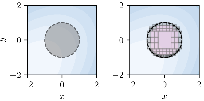
Illustration of the interval boxes produced with the constraint solver (RealPaver)

Stratified sampling with interval constraint propagation can lead to a significant variance reduction in the aggregated estimate by reducing the uncertainty only to the regions of the domain enclosed within the outer boxes, potentially avoiding sampling from large regions of the domain that can be analytically determined as including only or no solutions. Because boxes can be iteratively refined up to arbitrary accuracy, there is a trade-off between the target size (and, consequently, weight) of the boxes and their number (since each outer box requires a Monte Carlo estimation process).

Example. Consider the constraint $x^{2}+y^{2}\leq 1$ from the example in LABEL:listing:safety (variable names abbreviated). Performing interval constraint propagation with RealPaver (Granvilliers and Benhamou, 2006) – an interval constraint solver supporting conjunctive, nonlinear inequality constraints used in qCoral – with the initial input domain $x,y\in[-2,2]$, we obtained the outer and inner boxes depicted in Figure 1 in gray and pink, respectively.

In Figure 1, a large region of the domain falls outside the boxes since it contains no solutions. Hence, the probability of satisfying the constraint for values in this region is $0$. Similarly, the probability of satisfying the constraint with inputs from an inner box is $1$. Therefore, uncertainty is bounded within the outer boxes, and estimation proceeds sampling from their truncated distributions and aggregating the result via stratified sampling.

2.3. Limitations of qCoral

qCoral can produce scalable and accurate estimates for the satisfaction probability for constraints that 1) have low dimensionality or can be reduced to low-dimensional subproblems via constraints slicing, 2) are amenable to scalable and effective interval constraint propagation, and 3) whose input distribution have CDFs in analytical form and allows efficient sampling from their truncated distributions. These constraints typically do not hold for high-dimensional and correlated input distributions.

Constraint slicing assumes that all the inputs are probabilistically independent, with dependencies among variables arising only from computational operations (e.g. $\texttt{if}\;(x+y>0){\dots}$ ). Support for correlated variables requires changing the dependency relation to include also all correlated variable pairs. This may reduce the effectiveness of constraint slicing in reducing the dimensionality of the integration problems.

Interval constraint propagation contributes to reducing estimation variance by pruning out large portions of the input domain that do not contain solutions of a constraint and producing small-size outer boxes to bound the variance propagated from in-box local estimates. However, the complexity of this procedure grows exponentially with the dimensionality of the problem, rendering it ineffective when, after constraint slicing, the number of variables appearing in an independent constraint is still large, e.g. due to correlated inputs that cannot be separate. The effectiveness of interval constraint propagation for nonlinear, non-convex constraints also varies significantly for different formulations of the constraint (e.g. $x^{2}$ vs. $x\times x$) and may require manual tuning for optimal results (Granvilliers and Benhamou, 2006).

Stratified sampling requires analytical solutions of the input CDFs, as well as the ability to sample from truncated distributions. Both requirements are generally unsatisfiable for correlated input variables, whose CDF cannot be computed in closed form. The lack of an analytical CDF would require a separate Monte Carlo estimation problem to quantify the probability mass enclosed within each box and an analysis of how the corresponding uncertainty propagates through the stratified sampling and the composition operators of qCoral. Additionally, sampling from a truncated distribution typically relies on the computation of both the CDF and the inverse CDF of the original distribution, which is inefficient without an analytical form of these functions.

In summary, the main variance reduction strategies of qCoral based on interval constraint propagation and stratified sampling are not applicable for all but trivial correlated input distributions. Constraint slicing can be extended with probabilistic dependencies among input variables, but this results in smaller dimensionality reduction, with exponential impact on interval constraint propagation even when the CDFs of correlated inputs can be computed analytically.

2.4. Importance Sampling

The indicator function in Equation (2) return 1 only within the regions of the input domain satisfying a constraint (e.g. only within the circle in Figure 1). When this region encloses only a small probability mass, direct Monte Carlo methods sampling from the input distribution $p(\boldsymbol{x})$ may struggle to generate enough samples that satisfy the constraint, and therefore fail to estimate the quantity of interest $p_{PC}$. We discussed before how qCoral uses interval constraint propagation and stratified sampling to prune out regions of the domain that contain no solutions, sampling within narrower boxes containing a larger portion of solutions.

An alternative method to improve statistical inference in this problem is importance sampling (IS). Instead of sampling from the input distribution $p(\boldsymbol{x})$, IS generates samples from a different proposal distribution – $q(\boldsymbol{x})$ – that overweighs the important regions of the domain, i.e., the regions containing solutions in our case. Because the samples are generated from a different distribution than $p(\boldsymbol{x})$, the computed statistics need to be re-normalized as in Equation 4:

(4) $$p_{PC}:=\int_{\boldsymbol{x}}\mathds{1}_{PC}(\boldsymbol{x})p(\boldsymbol{x})\,d\boldsymbol{x}=\int_{\boldsymbol{x}}\frac{\mathds{1}_{PC}(\boldsymbol{x})p(\boldsymbol{x})}{q(\boldsymbol{x})}q(\boldsymbol{x})\,d\boldsymbol{x}$$

(5) $$\approx\frac{1}{N}\sum_{i=1}^{N}\frac{\mathds{1}_{PC}(\boldsymbol{x}^{(i)})p(\boldsymbol{x}^{(i)})}{q(\boldsymbol{x}^{(i)})}=:\hat{p}^{IS},\;\text{where}\,\boldsymbol{x}^{(i)}\sim q(\boldsymbol{x}).$$

While any distribution $q(\boldsymbol{x})>0$ over the entire domain guarantees the estimate will eventually converge to the correct value, an optimal choice of $q(\boldsymbol{x})$ determines the convergence rate of the process and its practical efficiency. In our context of estimating the probability of satisfying path conditions $PC$, the optimal proposal distribution $q^{*}(\boldsymbol{x})$ is exactly the truncated, normalized distribution $p(\boldsymbol{x})$ satisfying $PC$,

$$q^{*}(\boldsymbol{x})=\frac{1}{p_{PC}}p(\boldsymbol{x})\mathds{1}_{PC}(\boldsymbol{x}).$$

In general, it is infeasible to sample from $q^{*}(\boldsymbol{x})$ as it requires the calculation of $p_{PC}$ which is exactly our target. Fortunately, as we will demonstrate in Section 3.1, a proposal distribution found via adaptive refinement can allow us to achieve near-optimal performance.

In this paper, we propose a new inference method to estimate the satisfaction probability of numerical constraints on high-dimensional, correlated input distributions. Our method does not require analytical CDFs and can replace qCoral’s variance reduction strategies to analyze constraints where these are not applicable. Our method combines results from constraint solving and adaptive estimation to produce near-optimal proposal distributions aiming at computing high-accuracy estimates suitable for the analysis of low-probability constraints.

3. SYMPAIS: SYMbolic Parallel Adaptive Importance Sampling

In this section, we introduce our new solution space quantification method for probabilistic program analysis: SYMbolic Parallel Adaptive Importance Sampling (SYMPAIS).

Figure 2. Overview of SYMPAIS.

[Overview of SYMPAIS]Overview of SYMPAIS.

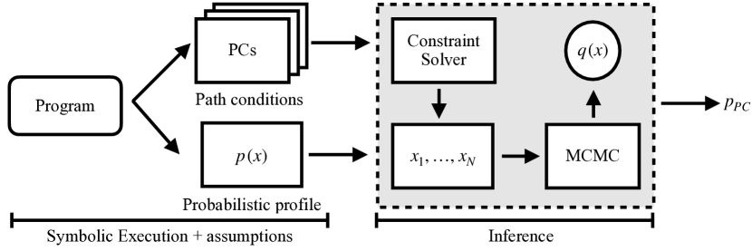
Figure 2 gives an overview of SYMPAIS’s workflow. Following the probabilistic symbolic execution approach, the path conditions leading to the occurrence of a target event are extracted using a symbolic execution engine. For simplicity, we assume that each (vector of) symbolic variables is associated with a probability distribution, either provided explicitly by the user or extracted from the code, where it has been specified via convenient random generators. Independent variables are associated with univariate probability distributions. Vectors of correlated variables are associated with multivariate probability distributions. For example, in LABEL:listing:safety, altitude is associated with a univariate Gaussian distribution with location $8000$ and scale $500$, while $<\texttt{obstacle\_x},\texttt{obstacle\_y}>$ are distributed as a bivariate Gaussian with location $[-2,-2]$ and covariance matrix $[[0.1,0.1],[0.1,0.2]]$. The path conditions are assumed to have been sliced as in (Filieri et al., 2013; Borges et al., 2014), where the dependency relation is augmented with pairwise dependency between the correlated variables, besides the dependencies induced by the program control and data flows. The probability of satisfying each independent constraint is quantified in the inference phase, which is the focus of this work.

Algorithm 1 Symbolic Parallel Interacting Markov Adaptive Sampling (SYMPAIS)

1:Given $C,p(\boldsymbol{x})$ $\triangleright$ SymEx(P), domain knowledge

2:$\overline{p}(\boldsymbol{x})\leftarrow p(\boldsymbol{x})\mathds{1}_{C}(\boldsymbol{x})$

3:$\boldsymbol{x}_{\texttt{init}}\leftarrow models(C)$$\triangleright$ Constraint solver

4:Initialize the proposal distribution $q_{n,0}$ for $n=1,\dots,N$.

5:for $t\leftarrow 1,\dots,T$ do$\triangleright$ Run PI-MAIS for $T$ iterations

6:     Update $N$ proposal distributions $q_{1:N,t}$ using MCMC

7:     Draw $M$ samples from each proposal distribution,

(6) $$\boldsymbol{x}^{(m)}_{n,t}\sim q_{n,t}(\boldsymbol{x}),\quad\text{for}\;m=1:M,\text{and}\,n=1:N.$$

8:     Compute importance-sampling weights,

(7) $$w_{n,t}^{(m)}\leftarrow\frac{\overline{p}(\boldsymbol{x}_{n,t}^{(m)})}{\frac{1}{N}\sum_{j=1}^{N}{q_{j,t}(\boldsymbol{x}_{n,t}^{(m)})}}$$

9:end for

10:Obtain PI-MAIS esitmate,

(8) $$\hat{p}_{\text{PIMAIS}} \leftarrow\frac{1}{T\cdot N\cdot M}\sum_{t=1}^{T}\sum_{n=1}^{N}\sum_{m=1}^{M}w^{(m)}_{n,t},$$

(9) $$\hat{v}^{2}_{\text{PIMAIS}} \leftarrow\frac{1}{T\cdot N\cdot M}\sum_{t=1}^{T}\sum_{n=1}^{N}\sum_{m=1}^{M}(w^{2(m)}_{n,t}-\hat{p}_{\text{PIMAIS}})^{2}$$

11:return $\hat{p}_{\text{PIMAIS}}$, $\hat{v}^{2}_{\text{PIMAIS}}$

The main steps of SYMPAIS are summarized in Algorithm 1. SYMPAIS takes as input a constraint $C$, which may be a path condition of $P$ or an independent portion of the path condition after constraint slicing, $C$ is assumed to be the conjunction of inequalities (or equalities) on numerical functions of the inputs. In addition to the constraint $C$, SYMPAIS requires specifying a probability distribution $p(\boldsymbol{x})$ over the symbolic variables in the program. Such distribution can be provided by the user or specified in the code via convenient random generators. For simplicity, we refer to the probability distribution over all of the symbolic variables as the input distribution.

Overview. The core part of SYMPAIS is the adaptive importance sampling process implemented in the for loop at 5. The goal of this process is to iteratively refine an importance sampling proposal that maximizes sample efficiency, i.e., it is very likely to generate sample points within the solution space of the input constraint $C$. Due to the wide range of possible constraint forms (e.g. linear, non-linear, non-convex) and of different types of distributions, optimal proposal distributions cannot be obtained analytically. It is instead approximated via a hierarchical probability distribution whose parameters are iteratively refined via a Markov Chain Monte Carlo (MCMC) algorithm (Metropolis et al., 1953; Neal, 2011) to best approximate the intractable optimal proposal. MCMC algorithms generate sequences of samples that, when the process converges to its steady state, the samples are distributed according to a target distribution whose analytical form may be unknown or from which it is not possible or intractably complex to sample directly. The MCMC samples can thus be used to iteratively estimate the parameters of the proposal distribution towards approximating the optimal distribution. The algorithm returns the estimate of the satisfaction probability, as well as the estimator variance. The latter may be used to reason about the dispersion of the estimate, e.g., constructing confidence intervals to decide if more sampling is desirable. Notice however that, similarly to qCoral (Borges et al., 2014), the estimator variance is centered around the estimate (Formula (9) in Algorithm 1). This requires enough samples to have been collected for the estimate to stabilize first in order for the variance to represent the estimator dispersion around it.

In the remaining of the section (Section 3.1), we will formally define the adaptive importance sampling strategy of SYMPAIS and the MCMC methods it adopts for the adaptive refinement of the proposal distribution. Results from constraint solving will be brought in to mitigate the complexity of the estimation process and accelerate its convergence. A set of optimizations to improve the practical performance of the methods will be discussed in Section 3.2, while implementation details and an experimental evaluation will be reported in Section 4.

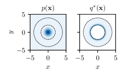
Running example. To illustrate the different features of SYMPAIS, we will use a 3-dimensional, nonlinear and non-convex constraint – torus –, which is defined in Equation (10):

(10) $$(\sqrt{x^{2}+y^{2}}-R)^{2}+z^{2}\leq r^{2},$$

with the constant parameters $R=3$, $r=1$. At first, we will associate to each of the three variables an independent univariate Gaussian distribution: i.e., $x,y,z\sim{\mathcal{N}}(0,0.5)$. We will later generalize the method to correlated inputs.

3.1. SYMPAIS Adaptive Importance Sampling

As recalled in Section 2.4, importance sampling (IS) methods aim at constructing a proposal distribution $q(\boldsymbol{x})$ that increases the likelihood of generating samples that satisfy a constraint $C$. This allows us to focus the estimation problem to the regions of the input domain that satisfy $C$, while avoiding the need to find a stratification of the input domain and computing the inverse CDFs for the distribution truncation that prevent the use of qCoral for high-dimensional and correlated input distributions.

Figure 3. Left: input distribution $p(\boldsymbol{x})$ for torus projected on the x-y plane. Right: the optimal importance sampling proposal $q^{*}(\boldsymbol{x})$. The intensity of the blue shadowing is proportional to the probability density. The solution space lays between the dashed circles.

Visualizing the input distribution and optimal proposal

The choice of a proposal distribution $q(\boldsymbol{x})$ largely affects the efficiency of IS. However, it is usually difficult to obtain an analytical form for the theoretically optimal $q^{*}(\boldsymbol{x})$ or to sample from. Instead, we use an adaptive scheme to iteratively refine a proposal distribution to approximate $q^{*}(\boldsymbol{x})$.

3.1.1. Adaptive proposal refinement

To construct and refine the IS proposal distribution, SYMPAIS adapts the parallel interacting Markov adaptive sampling (PI-MAIS) schema defined in (Martino et al., 2017). The proposal distribution in PI-MAIS is a hierarchical model parameterized by $N$ sub-proposals $q_{1},\dots,q_{N}$. To sample from the proposal distribution, we first choose a sub proposal $q_{i}$ and then draw samples $\boldsymbol{x}$ from $q_{i}$. Together, the sub-proposals form a mixture distribution. PI-MAIS adapts the sub-proposals to the target distribution by running parallel-chain MCMC (Line 6) so that it can form efficient proposal distributions for target distributions that are multimodal and non-linear.

In this paper, we use sub-proposals parameterized by Gaussian distributions $q_{i}(\boldsymbol{x})={\mathcal{N}}(\boldsymbol{x};\boldsymbol{\mu}_{i},\Sigma)$. The probability density function (PDF) for the proposal distribution is then given by a Gaussian:

$$q(\cdot)=\frac{1}{N}\sum_{i=1}^{N}{\mathcal{N}}(\cdot,\boldsymbol{\mu}_{i},\Sigma),$$

where the mean vectors $\left\{\boldsymbol{\mu}_{i}\right\}_{i=1}^{N}$ are adapted by running $N$ parallel MCMC samplers so that the proposal distribution approximates more accurately $q^{*}(\boldsymbol{x})$. At each step $t$, a sampler produces a set of samples $\{\boldsymbol{x}_{n,t}\}$. The proposal distribution at step $t$ is:

$$q_{t}(\cdot)=\frac{1}{N}\sum_{n=1}^{N}q_{n,t}(\cdot)=\frac{1}{N}\sum_{n=1}^{N}{\mathcal{N}}(\cdot|\boldsymbol{x}_{n,t},\Sigma).$$

When the refinement process stabilizes, the estimate for the probability of satisfying the constraint $C$ given the input distribution $p(\boldsymbol{x})$ (i.e., the solution of the integration problem in Equation (1)) is:

$$\hat{p}^{PIMAIS}\approx\frac{1}{T}\frac{1}{N}\frac{1}{M}\sum_{t=1}^{T}\sum_{n=1}^{N}\sum_{m=1}^{M}w_{t,n,m},\,w_{t,n,m}=\frac{\overline{p}(\boldsymbol{x}^{(m)}_{n,t})}{q_{t}(\boldsymbol{x}^{(m)}_{n,t})},$$

where $\boldsymbol{x}^{(m)}_{n,t}$ are samples drawn from $q_{n,t}(\boldsymbol{x})$. Please refer to (Martino et al., 2017) for the convergence proofs of the PI-MAIS scheme.

To update the proposal distribution, we implemented two MCMC samplers in SYMPAIS: random-walk Metropolis-Hastings (RWMH) and Hamiltonian Monte Carlo (HMC). The former provides a general procedure that only requires the ability to evaluate the density of the constrained input distribution $\bar{p}(\boldsymbol{x})=p(\boldsymbol{x})\mathds{1}_{C}$ for a given value $\boldsymbol{x}$. The latter requires the $p(x)$ to be differentiable and exploits the gradient information to achieve higher efficiency in many cases, especially for higher dimensional problems. For space reason, in the remainder of this section we will mostly focus on RWMH while additional details on our HMC implementation are provided in (Luo et al., 2021).

Random-Walk Metropolis-Hasting for adaptation.

MCMC methods generate a sequence of samples where each sample is via a probabilistic transition from its predecessor. Random-Walk Metropolis-Hasting (RWMH) (Owen, 2013; Metropolis et al., 1953) is an MCMC algorithm where the next sample $\boldsymbol{x}^{\prime}$ is generated from its predecessor $\boldsymbol{x}$ from a proposal distribution (or proposal kernel) $\kappa(\boldsymbol{x}^{\prime}|\boldsymbol{x})$. The newly proposed sample $\boldsymbol{x}^{\prime}$ is accepted and added to the sequence randomly with probability $\alpha=\min\left(1,\frac{\overline{p}(\boldsymbol{x}^{\prime})\kappa(\boldsymbol{x}\mid\boldsymbol{x}^{\prime})}{\overline{p}(\boldsymbol{x})\kappa(\boldsymbol{x}^{\prime}\mid\boldsymbol{x})}\right)$, otherwise the new sample is rejected and $\boldsymbol{x}$ is retained.

For RWMH within SYMPAIS, we use $\kappa(\boldsymbol{x}^{\prime}|\boldsymbol{x})={\mathcal{N}}(\boldsymbol{x}^{\prime};\boldsymbol{x},\Sigma)$, i.e., the next candidate sample is generated by adding a white Gaussian noise with covariance $\Sigma$ to the current sample $\boldsymbol{x}$. After the generation process converges at steady state, a value $\boldsymbol{x}$ should appear in the sequence with a frequency proportional to its probability in the target distribution $\overline{p}(\boldsymbol{x})$. Because $\overline{p}(\boldsymbol{x})$ is zero outside the solution space of the constraint $C$, all the samples that do not satisfy $C$ will be rejected. High rejection rate slows down the convergence and can be mitigated by tuning $\Sigma$, using a different proposal kernel (Owen, 2013), or switching to more sophisticated methods to generate the next sample, such as a Hamiltonian proposal.

3.1.2. SYMPAIS estimation process

Each of the parallel MCMC processes used to refine the importance sampling proposal requires an initial value $\boldsymbol{x}_{init}$ to start from. In theory, any point from the input domain can be chosen to start the MCMC processes. However, principled choices of $\boldsymbol{x}_{init}$ can speed up the converge of the Markov chain to a steady state and reduce the sample rejection rate. The choice of the initial points is particularly important when the constrained distribution $\overline{p}(\boldsymbol{x})$ is multimodal – i.e., its density function has two or more peaks –, either because the original input distribution $p(\boldsymbol{x})$ is itself multimodal or because the restriction to the solution space of $C$ induces multiple modes in $\overline{p}(\boldsymbol{x})$. We will discuss the problem of multiple modes and SYMPAIS’s mitigation strategies in Section 3.2 while focus here on SYMPAIS’s use of constraint solving to initialize the MCMC processes.

In statistical inference literature, the initial sample of an MCMC process is typically randomly assigned by a value within the input domain. However, if the satisfaction probability of the constraint $C$ is small, randomly generating a value of $\boldsymbol{x}$ that satisfies the constraint may require a large number of attempts. Instead, we use a constraint solver (Z3 (de Moura and Bjørner, 2008) in this work) to generate one or more models for the constraint $C$ to seed the MCMC processes.

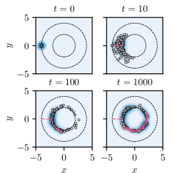
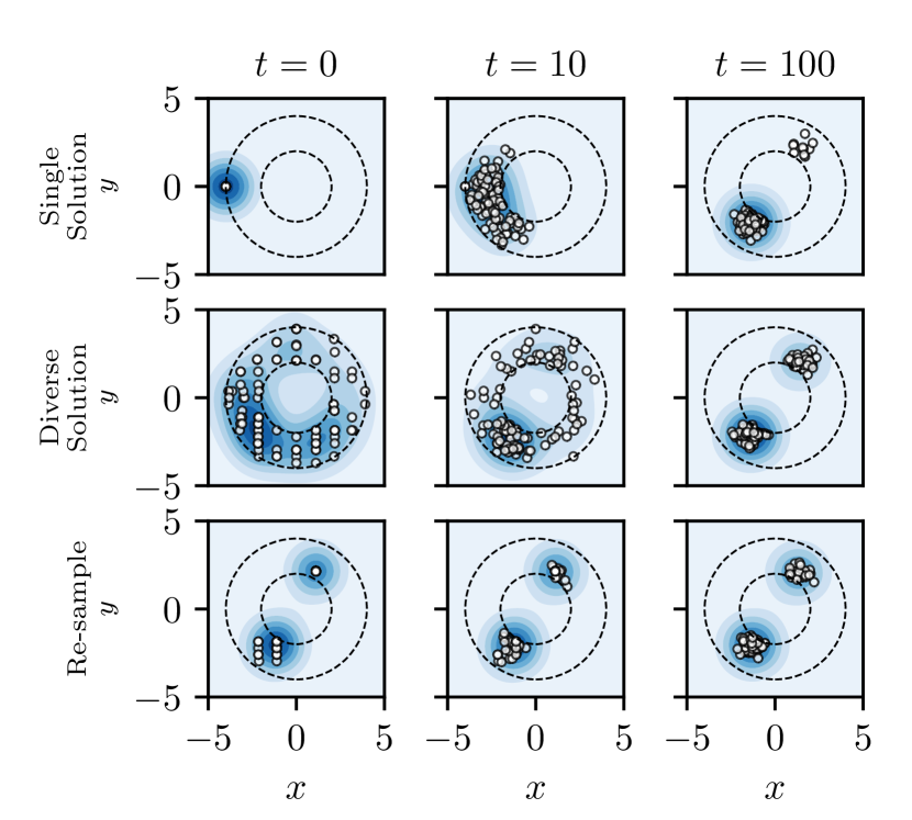
. [Graphical illustration of learning the adaptive proposal in SYMPAIS.]Graphical illustration of learning the adaptive proposal in SYMPAIS.

Figure 4. Graphical illustration of learning the adaptive proposal in SYMPAIS.

Figure 4 demonstrates visually the evolution of the proposal distribution through the iterations of the SYMPAIS loop (Line 5) towards the optimal proposal distribution depicted in Figure 3. We use a projection of the torus constraint on the x-y plane again as an example. At the beginning ($t=0$), the process is initialized with a solution produced by Z3. The importance sampling proposal distribution is concentrated around that point, where darker shadows of blue represent higher probability density. At iteration $t=10$, the proposal distribution translated towards the inner border of the solution space, where the constrained input distribution $\overline{p}(\boldsymbol{x})$ has a higher density. The white dots represent the samples $\boldsymbol{x}_{n,t}$ from the MCMC processes that are also used to refine the mean vectors of the importance sampling proposal $q_{n,t}$. Proceeding through the iterative refinement, at iteration $t=1000$ the proposal distribution approximates the optimal proposal very closely. The red line in the rightmost subfigure shows a trajectory – a sequence of values – generated by one of the MCMC processes, which touches portions of the solution space approximately proportionally to their density in the optimal distribution.

The accurate approximation of the optimal proposal distribution allows SYMPAIS to effectively sweep the solution space of $C$ and estimate its satisfaction probability.

Correlated input distributions. The adaptive importance sampling strategy, as well as the MCMC processes described in this section, do not require the input distributions to be independent. Correlated distributions (such as the bivariate Gaussian in LABEL:listing:safety) can be seamlessly processed by SYMPAIS. The requirement for RWMC is the ability to evaluate the PDF of the distribution, while HMC requires its differentiability. Computing the CDF (and its inverse) as required for qCoral’s stratified sampling does instead involve an integration problem that usually has no analytical solution and requires a separate Monte Carlo integration. SYMPAIS thus complements qCoral to allow the probabilistic analysis of a broader range of programs. We will demonstrate applications of SYMPAIS to correlated input distributions in Section 4.

3.2. Optimizations

The target distribution of SYMPAIS is $\overline{p}(\boldsymbol{x})=p(\boldsymbol{x})\mathds{1}_{PC}(\boldsymbol{x})$, where the indicator function zeroes the input distribution’s density outside the solution space of $C$. However, the MCMC processes are not aware of the geometry or location of the solution space of $C$. The volume and shape of the solution space may affect the rejection rate of the processes – how often the random walk reaches non-solution points – and may induce multiple modes in $\overline{p}(\boldsymbol{x})$ even if $p(\boldsymbol{x})$ is unimodal. Intuitively, each mode is a peak in the density function of $\overline{p}(\boldsymbol{x})$, which behaves as an attractor for the MCMC processes, requiring a longer time to converge to covering all the modes.

Example. Figure 5 shows how the optimal proposal distribution $q^{*}(\boldsymbol{x})$ for a unimodal, correlated input distribution $p(\boldsymbol{x})$ – we used a Student’s T distribution with 2 degrees of freedom for the plot – degenerates into a bimodal optimal proposal when constrained within the solution space of $C$ (torus constraint projected to the x-y plane). An MCMC process initialized in the neighborhood of one of the mode may take a long time before “jumping” in the neighborhood of the other mode, having to traverse a low probability path across the non-convex solution space.

Figure 5. Left: unimodal correlated input distribution $p(\boldsymbol{x})$. Right: optimal bi-modal proposal distribution $q^{*}(\boldsymbol{x})$.

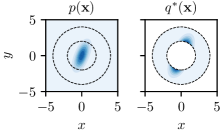
Illustration of the input distribution and optimal proposal distribution.

While a complete characterization of $C$’s geometry is intractable, in this section, we propose three heuristic optimizations that may mitigate the impact of ill geometries of the solution space on SYMPAIS adaptive importance sampling.

3.2.1. Diverse initial solutions.

For an effective importance sampling, the adaptive proposal distribution should capture all the modes of $q^{*}(\boldsymbol{x})$. Running multiple MCMC processes in parallel increases the chances of at least any of them covering each mode. In the statistical inference literature, each chain is typically initialized with an independent random sample from the input distribution to maximize the chances of reaching all the modes on the whole. However, as discussed before, if the satisfaction probability of $C$ is small, it is unlikely to randomly generate valid solutions and even less likely to also cover multiple modes.

Initializing all the chains with a feasible solution generated by the constraint solver may result in the MCMC processes exploring, in a finite time, only the mode closest to the initial solution. We observed this phenomenon in particular for RWMH, but multimodal distributions require longer convergence times also with HMC. The top row in Figure 6 shows the evolution of the adaptive importance sampling proposal $q(\boldsymbol{x})$ of SYMPAIS initialized with a single solution from the constraint solver. This time, the optimal proposal distribution $q^{*}(\boldsymbol{x})$ is the one on the right-hand side of Figure 5. After $t=100$ iterations, $q(\boldsymbol{x})$ still fails to converge to $q^{*}(\boldsymbol{x})$, with most of the samples still generated around one of the two modalities – which have instead the same density in $q^{*}(\boldsymbol{x})$.

Figure 6. Convergence of the adaptive proposal distribution with different initialization strategies.

Convergence of the adaptive proposal distribution with different initialization strategies.

To mitigate this problem, SYMPAIS tries to generate multiple diverse solutions of $C$ to increase the probability of obtaining at least one in the neighborhood of each mode. We explored two different approaches for this purpose. In principle, initial solutions diversity can be achieved using an optimizing solver where each solution is chosen to maximize the distance from all the previous ones. This method is general and flexible (e.g. it allows customizing the distance function based on domain-specific information), but computationally heavy for non-linear, non-convex constraints.

An alternative, more scalable method relies on interval constraint propagation and branch and bound algorithms to single out regions of the input domain that satisfy $C$. In our implementation, we use RealPaver’s depth-first search mode with a coarse accuracy (Granvilliers and Benhamou, 2006) ($10^{-2}$ in this example, but the configuration can be tuned based on the length of the domain dimensions) to generate several boxes that contain solutions of $C$. This mode differs from the standard paving used in qCoral because it does not require the computed boxes enclosing all the solutions, but potentially only a subset of them, making it more scalable even for higher-dimensional problems. For each box, SYMPAIS calculates the center and, if it satisfies $C$, adds it to the MCMC initialization points.

An example of the SYMPAIS adaptive proposal distribution using this heuristic is shown in the middle row of Figure 6. The initial solutions cover, with different concentrations, several parts of the solution space of $C$. While the initial iterations result in a very spread proposal $q(\boldsymbol{x})$ – contrary to the highly concentrated optimal proposal – the diversity of the initial points allows the adaptive refinement to converge to covering both optimal proposal’s modes.

While the heuristics of using depth-first interval constraint propagation may fail to produce solutions at the center of its boxes, or to refine the boxes enough for it to happen, when applicable, it is an efficient alternative to solving heavier optimization problems.

3.2.2. Re-sampling

The diversification of the initial solutions described in the previous section uses only information about the constraint to generate diverse initial points. However, the constraint solver is not aware of the underlying input distribution and may generate many solutions that are far from the modes of $q^{*}(\boldsymbol{x})$. When the $N$ parallel MCMC processes are initialized with solutions taken uniformly at random from those generated by constraint solver, many of these solutions are likely to be far from the modes, therefore requiring longer warmup of the Markov chains to move towards the modes. This can be observed in the wide spread of the proposal $q(\boldsymbol{x})$ for $t=0,10$ in the middle row of Figure 6.

To reduce the number of samples used for warmup, we sample the initial solutions proportionally to their likelihood in the input distribution. Let $\{\boldsymbol{x}_{i}\}_{i=1}^{F}$ be the initial solutions found by the constraint solver. We sample $N$ initial points $\{\boldsymbol{x}^{\prime}_{i}\}_{i=1}^{N}$ from

$$q(\boldsymbol{x}^{\prime})=\sum_{i=1}^{F}w_{i}\,\delta_{\boldsymbol{x}_{i}}(\boldsymbol{x}^{\prime}),\quad w_{i}=p(\boldsymbol{x}_{i})/\sum_{j=1}^{F}p(\boldsymbol{x}_{j}),$$

to be the initial states for the $N$ parallel MCMC chains.

The initial solutions seeding the MCMC chains now reflect both the location of the solutions space – from the constraint solver – and the distribution of the input probability across the solution space – from the resampling. An example of the effects on the convergence speed of SYMPAIS adaptation is shown in the bottom row of Figure 6.

3.2.3. Truncated kernel for RWMH

The proposal kernel for RWMH defined in the previous section generates the next sample by adding Gaussian noise to the current one: $\kappa(\boldsymbol{x}^{\prime}|\boldsymbol{x})={\mathcal{N}}(\boldsymbol{x}^{\prime};\boldsymbol{x},\Sigma)$. While arbitrarily concentrated around $\boldsymbol{x}$ by the value of $\Sigma$, this kernel may propose new samples far away from the solution space of $C$, which would then be rejected.

A way to reduce the rejection rate is to replace the kernel with a Gaussian noise truncated within a smaller region of the input domain that contains the solution space of $C$. We obtain this region in the form of the smallest n-dimensional box that contains $C$. Such a box can be efficiently computed when an interval contractor function is defined for $C$ (Araya et al., 2012). Efficient interval contractors are implemented for a broad class of numerical constraints, e.g.  (Goldsztejn and Chabert, 2021), and can be used to compute the smallest box $\mathcal{B}$ that encloses the solutions space of $C$. The Gaussian proposal kernel of RWMH can then also be replaced by the truncated Gaussian proposal kernel $\kappa_{\mathcal{B}}(\boldsymbol{x}^{\prime}|\boldsymbol{x})={\mathcal{N}}_{\mathcal{B}}(\boldsymbol{x}^{\prime};\boldsymbol{x},\Sigma)$ to increase the probability of generate candidate samples $\boldsymbol{x}^{\prime}$ that are still solutions of $C$.

Notice that this optimization does not require us to truncate the input distribution $p(\boldsymbol{x})$, as required by qCoral. Instead, it truncates the uncorrelated Gaussian distribution of the proposal kernel of RWMH, which can be done efficiently. Notably, the rejection rate does not go to zero because $\mathcal{B}$ may be a coarse bounding of the solution space of $C$, which may also be non-convex. Nonetheless, it usually increases the probability of sampling solutions of $C$.

4. Evaluation

In this section, we report an experimental evaluation of SYMPAIS. We include direct Monte Carlo (DMC) estimation as a baseline, qCoral for the uncorrelated input distributions, and SYMPAIS and SYMPAIS-H where we configure SYMPAIS to use the RWMH and the HMC algorithms for the MCMC samples, respectively. We include two geometrical microbenchmarks to expose the features of SYMPAIS and six benchmarks from path conditions extracted from a ReLU neural network and subjects from qCoral. Because the dependability of Monte Carlo estimators’ variance depends on the convergence of their estimates (cf. Section 3, overview), we use the relative absolute error (RAE) to compare the estimates against the ground truth, instead of performing statistical tests on the variance that are particularly challenging with the rare events considered in this paper. Details about the experimental environment and set-up are available in the extended version (Luo et al., 2021). Code is available at (Luo and Filieri, 2021).

4.1. Geometrical Microbenchmarks

4.1.1. Sphere

The first constraint we consider the d-dimensional sphere: $C:=\left\{\left\lVert\boldsymbol{x}-\boldsymbol{c}\right\rVert^{2}\leq 1\right\}$, where $\boldsymbol{x}\in[-10,10]^{d}\cap\mathbb{R}^{d}$ is the input domain, and $\boldsymbol{c}\in\mathbb{R}^{d}$ is the center of the sphere. We use $p(\boldsymbol{x})={\mathcal{N}}(0,I)$ – i.e., uncorrelated Gaussian – as the input distribution and set $\boldsymbol{c}=\mathbf{1}$. Despite its simplicity, this problem illustrates the challenges faced by direct Monte Carlo methods as well as qCoral in high-dimensionality problems where $C$’s satisfaction probability is small.

Specifically, as $d$ increases, the probability of the event happening decreases, which makes estimation by DMC increasingly challenging. Moreover, the increase in $d$ also leads to coarser paving of $d$-dimensional boxes, which reduces the effectiveness of variance reduction via stratified sampling.

Figure 7. RAE and convergence rates for spheres of different dimensionality.

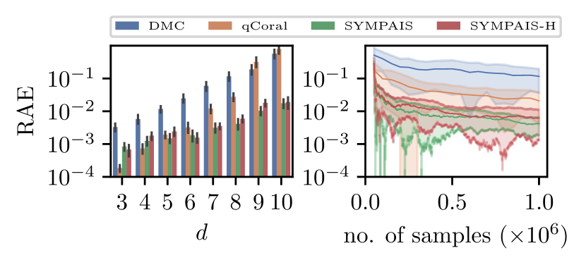
RAE and convergence rates for spheres of different dimensionality.

The RAE results are illustrated in Figure 7 (left). As expected: DMC achieves the worst performance throughout all tests. For low-dimensional problems ($d\leq 4$), qCoral is the most efficient, while its performance deteriorates significantly when the $d$ increases and RealPaver fails to prune out large portions of the domain that contain no solutions. SYMPAIS’s performance is comparable to qCoral in low dimensions, but up to one order of magnitude more accurate when the dimensionality grows ($d\geq 8$).

Figure 7 (right) shows the convergence rate of RAE for different methods over sample size for $d=8$. SYMPAIS achieves the final RAE of DMC with $<5\%$ of the sampling budget and the final RAE of qCoral with $<10\%$. SIMPAIS-H only marginally outperforms SYMPAIS for $8\leq d\leq 10$. The improvement in sample efficiency becomes more significant for $d>8$.

4.1.2. Torus

Torus is a three-dimensional constraint introduced in Section 3 as a running example. We evaluate the different methods for both independent and correlated inputs.

Independent inputs. We first consider the uncorrelated input distribution $p(\boldsymbol{x})={\mathcal{N}}(\mathbf{0},0.5\mathbf{I})$ with input domain $\boldsymbol{x}\in[-5,5]^{3}\cap\mathbb{R}^{3}$. Figure 8 (left) shows the RAE performance of the four methods. While performing marginally better than the baseline DMC, qCoral achieve poor performance on this non-convex subject because RealPaver fails to effectively prune out the inner empty region of the domain within the torus, effectively reducing qCoral to a DMC sampling over most of the input domain.

RealPaver can be fine-tuned for a torus constraints by using different consistency configurations (see (Granvilliers and Benhamou, 2006) for instructions on the matter). However, this may require human ingenuity to select and tune the correct settings. Finally, we observed the performance of RealPaver varies for equivalent formulations of the constraint (e.g., $x^{2}$ vs $x\times x$ or reformulating the constraint without $sqrt(\cdot)$). We conjecture that using different interval constraint propagation algorithms or clever simplifications of the constraint may improve the performance of qCoral for this problem. Both variations of SYMPAIS achieve an order of magnitude lower RAE.

Figure 8. RAE comparison for torus.

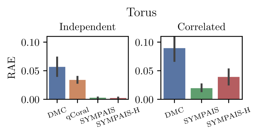
RAE comparison for torus.

Correlated inputs. Consider the correlated distribution

$$p(x,y,z)=\mathcal{T}_{2}(0,0.5){\mathcal{N}}(x,0.5){\mathcal{N}}(x,0.5),$$

where ${T}_{2}$ denotes a Student’s T distribution with 2 degrees of freedom. Similarly to the situation illustrated in Figure 5, the distribution constrained within the solution space of torus is bi-modal. In this case, the input distribution is correlated, with $y$ and $z$ probabilistically dependent on $x$.

Correlated and potentially multimodal input distributions are commonly used to describe real-world inputs arising from physical phenomena. More recently, the success of deep learning has encouraged incorporating deep neural networks for generative modeling of high-dimensional data distributions (Rezende and Mohamed, 2015; Rezende et al., 2014; Kingma and Welling, 2014), trained from observed data. For these distributions, the PDFs are often tractable, while CDFs often are not. This in turn makes the stratified sampling and truncations of the input distribution intractable for qCoral.

On the other hand, SYMPAIS can handle these problems because it only requires evaluating the PDF of the input distribution, not its CDF. Since qCoral cannot handle correlated inputs, Figure 8 (right) shows how both SYMPAIS and SYMPAIS-H outperforms the baseline DMC by nearly one order of magnitude. As discussed in Section 3.2, seeding the MCMC processes with re-sampled diverse solutions from the constraint solver improves SYMPAIS(-H)’s convergence for multimodal distributions as in this experiment.

4.2. ACAS Xu

Figure 9. RAE comparison for ACAS Xu activation patterns.

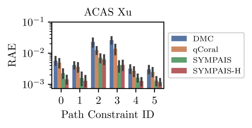
RAE comparison for ACAS Xu activation patterns.

ACAS Xu (Julian et al., 2016) is a benchmark neural network implementing a safety-critical collision avoidance system for unmanned aircraft control. Its inputs are readings from a set of sensors, including: distance from the other vehicle, angle of the other vehicles relative to ownship direction, heading angle of other vehicle, speed of ownship, and speed of the other vehicle. The outputs of the networks are either clear-of-conflict – no risk of collision between ownship and the other vehicle – or one of four possible collision avoidance maneuvers the ownship can take to avoid a collision. The US Federal Aviation Administration is experimenting with an implementation of ACAS Xu to evaluate its safety for replacing the current rule-based system (Converse et al., 2020).

This subject is has been used to benchmark several verification methods (e.g.  (Katz et al., 2017)), including performing a probabilistic robustness analysis that computes bounds on the probability of the network producing inconsistent decisions for small perturbations on the inputs (Converse et al., 2020). A central component of the analysis method in (Converse et al., 2020) consists of computing reliable bounds for the probability of satisfying a constraint that corresponds to a unique activation pattern of the network when white noise is added to an initial sensor reading.

For this experiment, we extract the constraints corresponding to six random activation patterns and estimate their satisfaction probability with different methods.

Consider a neural network with one hidden layer of $m$ neurons that receives input $\boldsymbol{x}\in\mathbb{R}^{d}$. The neural network computes the output as

$$\mathbf{z}=\mathbf{W}_{0}\boldsymbol{x}+\mathbf{b}_{0},\;\mathbf{a}=\operatorname{ReLU}(\mathbf{z}),\;\mathbf{y}=\mathbf{W}_{1}^{T}\mathbf{a}+\mathbf{b}_{1},$$

where $\operatorname{ReLU}$ is the Rectified Linear Unit defined as $\operatorname{ReLU}(\boldsymbol{x})=\max(0,\boldsymbol{x})$ evaluated component-wise on $\boldsymbol{x}$. $\mathbf{W}_{0},\mathbf{W}_{1},\mathbf{b}_{0}$ and $\mathbf{b}_{1}$ are the pre-trained weights of the neural network. A hidden unit $\mathbf{a}_{i}$ is active if the constraint $\mathbf{z}_{i}\geq 0$ is satisfied and inactive otherwise (i.e., $\mathbf{z}_{i}<0$). An activation pattern is defined as the conjunction of the activation constraints of the hidden units $\left\{\mathbf{a}_{i}\right\}_{i=1}^{m}$. We select the network with one hidden layer of five neurons for analysis (https://bit.ly/3fjAlOW). The selected network generates 32 possible combinations of activation patterns and we select randomly six activation patterns for analysis. We use ${\mathcal{N}}(0,1)$ to model the distribution of each input dimension $x_{i}$ of the neural network and additionally impose a domain of $[-100,100]\cap\mathbb{R}$ for each dimension. The bounded input and independent constraints allow the use of qCoral as well. However, neural networks tend to generate high-dimensional problems because they establish control dependencies among all their inputs, which prevents effective constraint slicing.

Figure 10. RAE achieved by the different methods on volComp subjects.

RAE achieved by the different methods on volComp subjects.

Figure 9 reports the RAE achieved by the different estimation methods for each of the six randomly sampled activation patterns. For this experiment, we used a single initial solution computed by Z3 to initialize the MCMC chains of SYMPAIS and SYMPAIS-H. Being the conjunction of ReLU activations, the constraints produced by ACAS Xu are convex (intersection of half-planes) and do not induce multiple modes on the constrained input distribution. Already using a single initial solution, SYMPAIS converged to better estimates than DMC and qCoral with the same sampling budget.

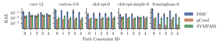
4.3. volComp

Finally, in this section we experiment with a set of constraints from the benchmark volComp (Sankaranarayanan et al., 2013), also used to evaluate qCoral (Borges et al., 2014, 2015). We picked the first five path conditions for each of the subjects named in Figure 10 from the public qCoral replication package. Because most of the input variables in these subjects are computationally independent, constraint slicing would reduce to constraints with dimensionality $<3$; we instead skip slicing and evaluate the original constraints having between 5 and 25 variables. The constraints are linear, with convex solution spaces. In this situation, RealPaver can produce a tight approximation of the solution space, with significant benefits for qCoral’s stratified sampling efficiency. The input CDF can be computed analytically (independent truncated Gaussian from qCoral’s replication package “normal”). Among the different experiments in (Borges et al., 2014), these subjects represent a sweet spot for the stratified sampling method of qCoral and are included here as SYMPAIS’s worst-case comparison scenario.

Our current implementation of the HMC kernel proposal does not support JIT-compilable truncated distributions. Thus we run only SYMPAIS with RWMH for this set of subjects.

Figure 10 shows the RAE of the different methods. The ground truth is computed with Mathematica. For all the subjects in this experiment, except cart-12, $99\%$ of the input domain enclosed within RealPaver’s boxes contains only solutions of the constraint. For all the subjects, except framingham-0, qCoral and SYMPAIS produce comparable RAE. A deeper inspection of framingham-0 showed that most of the constraint is effectively the intersection of boxes, which are identified as inner boxes by RealPaver and require no further sampling for probability estimation (Equation (3)). The experiment demonstrates that while the adaptive importance sampling strategy of SYMPAIS is designed to estimate the satisfaction probability of high-dimensional constraints with multimodal, correlated input distributions, it can match the performance of stratified sampling for most simpler problems where stratified sampling can be applied. The analysis of the same constraints with correlated inputs would instead not be possible with stratified sampling.

5. Related Work

Probabilistic symbolic execution (Geldenhuys et al., 2012) relies on symbolic execution to extract the path conditions characterizing the inputs that lead to the occurrence of a target event; the probability of satisfying the path condition constraints given an input distribution is then quantified using model counting or solution space quantification methods. PSE has been applied in several domains, including reliability (Filieri et al., 2013) security (Malacaria et al., 2018; Brennan et al., 2018) and performance analyses (Chen et al., 2016), with variations implemented for nondeterministic (Luckow et al., 2014) and probabilistic (Malacaria et al., 2018) programs. Quantification methods have been proposed for uniform or discretized distributions over linear integer constraints (Filieri et al., 2013), string constraints (Aydin et al., 2018), bounded data structured (Filieri et al., 2015), and numerical constraints over continuous input distributions (Borges et al., 2014, 2015).

In the probabilistic programming literature, Chaganty et al. (2013) proposed breaking a probabilistic program with branches and loops into small programs focused on only some execution paths and use pre-image analysis to perform efficient importance sampling. Differently from Chaganty et al. (2013), we use PI-MAIS and MCMC processes to further adapt the proposal distributions for the analysis of individual path conditions. Nori et al. (2014) similarly uses the idea of pre-image analysis to design a proposal distribution that generates samples that are less likely to be rejected in MCMC. These analyses complement our approach and can potentially be incorporated to improve our MCMC scheme. Recent work by Zhou et al. (2020) motivates the decomposition into subproblems by considering universal probabilistic programs with stochastic support, i.e., depending on the values of the samples, the program may take on different control-flow paths, and the number of random variables evaluated along each path varies as a result. This makes designing a proposal distribution for efficient MCMC difficult. Zhou et al. (2020) approaches this issue by decomposing the problem into small straight-line programs (SLPs) for which the support is fixed and posterior inference is tractable. However, differently from PSE approaches, SLPs are execution paths sampled via a specialized MCMC algorithm, which adds an additional degree of uncertainty to the results of probabilistic analysis and is not suitable for the analysis of rare events.

6. Conclusions and Future Work

We introduced SYMPAIS, a new inference method for estimating the satisfaction probability of numerical constraints on high-dimensional, correlated input distributions. SYMPAIS combines a sample-efficient importance sampling scheme with constraint solvers to extend the applicability of probabilistic symbolic execution to a broader class of programs processing correlated inputs that cannot be analyzed with existing methods. While we currently implemented only RWMH and HMC kernel as adaptive proposals, SYMPAIS can be extended with additional kernels to improve its performance on different classes of constraints. Finally, it is also worth investigating the integration of kernels and parametric importance sampling proposals for discrete distributions, aiming at supporting integer input variables that cannot be analyzed with our current algorithms.

Appendix

Appendix A Experimental settings details

Implementation. We implemented SYMPAIS in Python 3.8 using Google’s JAX framework (Bradbury et al., 2018) to implement the mathematical procedures and generate random samples. JAX provides automated differentiation, which we use for HMC, and allows for just-in-time compile the numerical routines of SYMPAIS for faster execution, mainly due to the use of its automatic vectorization features.

Execution environment. All the experiments have been run on an AMD EPYC 7401P CPU with 448Gb of memory. However, SYMPAIS was limited to using only two cores and never exceeded 4Gb of memory consumption in our experiments.

Configuration. The RWMH kernel is configured with scale $\sigma=1.0$. The HMC trajectory is simulated for $T=20$ steps, with each time step duration $\epsilon=0.1$; we use standard leapfrog steps to generate the Hamiltonian trajectory (Neal, 2011) (mathematical formulation in the Appendix). We use $N=100$ parallel MCMC chains. Each chain is warmed up with $500$ samples – i.e., $500$ samples are used to bring the chain near convergence and discarded; only the samples from the $501-th$ on are actually used. Overall, the $100$ chains take $50,000$ samples to warm up. For the RWMH kernel, we also implement adaptation of the scale parameter following in scheme used by PyMC3 (https://bit.ly/2HrpHJK).

For the adaptive importance sampling distribution $q_{n,t}(\cdot)$, we use ${\mathcal{N}}(\cdot|\boldsymbol{x}{n,t},0.5\Lambda)$ where $\Lambda$ is the covariance of the input distribution $p(\boldsymbol{x})$. For the input distributions where the covariance of $p(\boldsymbol{x})$ is analytically intractable, SYMPAIS uses the sample variance (estimated from $100$ samples). We draw $M=5$ samples from each sub-proposal $q_{n,t}$ during each iteration of the adaptation loop. RealPaver is configured with accuracy $0.1$ to generate the initial inputs of the MCMC chains and the truncated kernel proposal bounds (min/max over RealPaver’s boxes vertices). RealPaver for paving in qCoral computes up to 1024 boxes.

Experimental settings. We allow each of the four methods the same budget of $10^{6}$ samples. For SYMPAIS, this includes the samples used to warm up the MCMC chains and to estimate the covariance of the input distribution when not given. RealPaver executions for qCoral and SYMPAIS are not time-limited. However, all the experiments completed their execution within 2 minutes for the geometrical microbenchmarks and 5 minutes for the other subjects. The compilation time of JAX varies between $\tilde{2}0$ seconds and $\tilde{2}5$ minutes; reimplementing SYMPAIS with a compiled language might make the compilation time more predictable.

Each experiment is repeated $20$ times unless otherwise specified. To compare the estimates of the different methods, we use the relative absolute error (RAE) against a ground truth value computed with Mathematica (accuracy and precision goals = 15) or via a large direct Monte Carlo samples ($20\cdot 10^{8}$) for the geometrical microbenchmarks. The RAE is preferred to the absolute error because normalizing by the ground truth probability allows a homogenous comparison over constraints with different satisfaction probabilities.

Appendix B Hamiltonian Monte Carlo estimators

The Hamiltonian Markov Chain Monte Carlo (HMC) algorithm (Neal, 2011; Betancourt, 2018) uses derivatives of the target distribution and auxiliary variables to generate candidate samples more efficiently than RWMH when $p(\boldsymbol{x})$ is differentiable.

HMC generates the next sample $\boldsymbol{x}^{\prime}$ by simulating the movement of a particle pushed in a random direction starting from the location $\boldsymbol{x}$ across the surface defined by the probability density function of $p(\boldsymbol{x})$. Intuitively, regions where $p(\boldsymbol{x})$ is larger are at a “lower altitude” on the surface and are thus more likely to attract the particle. The random direction and energy of the push can allow the particle to reach any point of the surface. The position of the particle after a predefined fixed time $T$ will be the new candidate sample $\boldsymbol{x}^{\prime}$. A mathematical formulation of the HMC process implemented in SYMPAIS is reported in the Appendix, while for a broader presentation of the method, the reader is referred to (Betancourt, 2018).

To sample from the target distrbution of $\boldsymbol{x}$, HMC augments the original probability distribution $\overline{p}(\boldsymbol{x})$ with auxiliary momentum variables $\boldsymbol{\rho}$ and considers the joint density $\overline{p}(\boldsymbol{x},\boldsymbol{\rho})=p(\boldsymbol{\rho})\overline{p}(\boldsymbol{x})$ where $p(\boldsymbol{\rho}\nolinebreak\mid\boldsymbol{x})$ can be chosen as ${\mathcal{N}}(\mathbf{0},\mathbf{I})$, $\mathbf{I}$ being the identity matrix with size $|\boldsymbol{x}|$. Define the Hamiltonian $H$ as

$$H(\boldsymbol{x},\boldsymbol{\rho}) =-\log\overline{p}(\boldsymbol{x},\boldsymbol{\rho})$$

$$=-\log p(\boldsymbol{\rho})-\log\overline{p}(\boldsymbol{x})$$

$$=K(\boldsymbol{\rho})+U(\boldsymbol{x})$$

where $K(\boldsymbol{\rho})=-\log p(\boldsymbol{\rho})$ is called the kinetic energy and $U(\boldsymbol{x})=-\log\overline{p}(\boldsymbol{x})$ is called the potential energy.

A proposal $\boldsymbol{x}^{\prime}$ is made by simulating the Hamiltonian dynamics

$$\frac{d\boldsymbol{x}}{dt}=\nabla_{\boldsymbol{\rho}}K(\boldsymbol{\rho}),\;\frac{d\boldsymbol{\rho}}{dt}=-\nabla_{\boldsymbol{x}}U(\boldsymbol{x}),$$

which can be discretized and solved numerically by a symplectic integrator such as the Leapfrog method for $T_{\text{leapfrog}}$ steps with a step size of $\epsilon$

$$\boldsymbol{\rho}_{t+\epsilon/2} =\boldsymbol{\rho}_{t}-(\epsilon/2)\nabla_{\boldsymbol{x}}U(\boldsymbol{x}_{t}),$$

$$\boldsymbol{x}_{t+\epsilon} =\boldsymbol{x}_{t}+\epsilon\nabla_{\boldsymbol{\rho}}K(\boldsymbol{\rho}_{t+\epsilon/2}),$$

$$\boldsymbol{\rho}_{t+\epsilon} =\boldsymbol{\rho}_{t+\epsilon/2}-(\epsilon/2)\nabla_{\boldsymbol{x}}U(\boldsymbol{x}_{t+\epsilon})$$

for $t\in\{1,\dots,T_{\text{leapfrog}}\}$.

Choice of hyperparameters parameters such as the step size $\epsilon$ and the number of Leapfrog steps $T_{\text{leapfrog}}$ affects the efficiency of HMC methods. The No-U-Turn Sampler  (Hoffman and Gelman, 2014) is an extension to the HMC method which mitigates the effect of hyperparameter settings on HMC methods.

While potentially more efficient than RWMH, especially for higher-dimensional problems, – i.e., fewer candidate samples are rejected – HMC requires the target density function to be differentiable, which makes it less general than RWMH. In particular, it cannot be applied for input distribution with discrete parameters. Improvements to the original HMC algorithm and extensions exist to handle this limitation (Nishimura et al., 2020). Because SYMPAIS’s target distribution is $\bar{p}(\boldsymbol{x})=p(\boldsymbol{x})\mathds{1}_{C}$, instead of the original input distribution $p(\boldsymbol{x})$, the probability density is not differentiable at the boundary of the solution space of the constraint $C$, and simulations crossing that boundary have to be rejected. Extensions to HMC specialized for sampling from constrained spaces have been proposed for several classes of constraints and will be investigated for future extensions of SYMPAIS (Afshar and Domke, 2015; Betancourt, 2018; Nishimura et al., 2020; Neal, 2011).

Appendix C Additional discussion

Handling broader families of $p(\boldsymbol{x})$. Since SYMPAIS does not require CDF of $p(\boldsymbol{x})$ to be tractable, we only require that the PDF can be evaluated. This allows us to handle a broader family of distributions compared to qCoral. This is a trade-off between efficiency and generality. By assuming that the truncated CDF can be evaluated. qCoral can perform additional pruning that further eliminates probability masses where $\mathds{1}_{PC}(\boldsymbol{x})=0$. While stratified sampling can be used to reduce variance (Keramat and Kielbasa, 1998), most of the variance reduction in qCoral comes from pruning out irrelevant solution space instead of stratification. SYMPAIS, on the other hand, relaxes the assumption of having tractable truncated CDFs but instead reduces variance with IS. The interval contraction optimization allows us to reduce variance compared to AIS in the original space, but this can still produce a larger truncated proposal compared to qCoral. However, IS may provide additional variance reduction to compensate for the inefficiency in the stratified sampler in qCoral. In this case, SYMPAIS complements qCoral in situations where the stratification strategy is inefficient. When the truncated CDF is available, which method works better is likely problem-specific. In this case, the most practical solution is probably a combination of both. One can first do a preliminary run with a smaller number of samples to identify which method would work better and exploit the more efficient method.

Future improvements Improvements to the MCMC algorithm can improve SYMPAIS’s efficiency. In particular, it would benefit from improvements in MCMC that can explore multimodal posterior efficiently. Note that, however, the MCMC does not have to be perfect. For the PI-MAIS adaptation scheme, the crucial thing is that the parallel chains should capture the modes in $q^{*}(\boldsymbol{x})$ in a way the modes are relatively weighted in $q^{*}(\boldsymbol{x})$. This may explain why we do not observe improvements in performance when using the HMC kernel. Importance sampling can be dangerous if the adapted $q$ misses the modes of $q^{*}$; this is partly mitigated in SYMPAIS, which uses an adaptive mixture proposal that can approximate multimodal posteriors. Additionally, we plan to further improve the robustness of SYMPAIS against multimodal distributions adding supplementary diagnostics (e.g. Effective sample sizes (ESS)) and defensive importance sampling (Owen, 2013; Hesterberg, 1995).

References

- (1)
- Afshar and Domke (2015) Hadi Mohasel Afshar and Justin Domke. 2015. Reflection, Refraction, and Hamiltonian Monte Carlo. In Proceedings of the 28th International Conference on Neural Information Processing Systems - Volume 2 (NIPS’15). MIT Press, 3007–3015.
- Araya et al. (2012) Ignacio Araya, Gilles Trombettoni, and Bertrand Neveu. 2012. A Contractor Based on Convex Interval Taylor. In Integration of AI and OR Techniques in Contraint Programming for Combinatorial Optimzation Problems (Lecture Notes in Computer Science), Nicolas Beldiceanu, Narendra Jussien, and Éric Pinson (Eds.). Springer, 1–16. https://doi.org/10.1007/978-3-642-29828-8_1
- Aydin et al. (2018) Abdulbaki Aydin, William Eiers, Lucas Bang, Tegan Brennan, Miroslav Gavrilov, Tevfik Bultan, and Fang Yu. 2018. Parameterized Model Counting for String and Numeric Constraints. In Proceedings of the 2018 26th ACM Joint Meeting on European Software Engineering Conference and Symposium on the Foundations of Software Engineering. ACM, 400–410. https://doi.org/10.1145/3236024.3236064
- Betancourt (2018) Michael Betancourt. 2018. A Conceptual Introduction to Hamiltonian Monte Carlo. arXiv:1701.02434 [stat] (July 2018). arXiv:1701.02434 [stat]
- Borges et al. (2015) Mateus Borges, Antonio Filieri, Marcelo D’Amorim, and Corina S. Păsăreanu. 2015. Iterative Distribution-Aware Sampling for Probabilistic Symbolic Execution. In Proceedings of the 2015 10th Joint Meeting on Foundations of Software Engineering. ACM, 866–877. https://doi.org/10.1145/2786805.2786832
- Borges et al. (2014) Mateus Borges, Antonio Filieri, Marcelo d’Amorim, Corina S. Păsăreanu, and Willem Visser. 2014. Compositional Solution Space Quantification for Probabilistic Software Analysis. In Proceedings of the 35th ACM SIGPLAN Conference on Programming Language Design and Implementation. ACM, 123–132. https://doi.org/10.1145/2594291.2594329
- Bradbury et al. (2018) James Bradbury, Roy Frostig, Peter Hawkins, Matthew James Johnson, Chris Leary, Dougal Maclaurin, George Necula, Adam Paszke, Jake VanderPlas, Skye Wanderman-Milne, and Qiao Zhang. 2018. JAX: Composable Transformations of Python+NumPy Programs. https://github.com/google/jax
- Brennan et al. (2018) Tegan Brennan, Seemanta Saha, Tevfik Bultan, and Corina S. Păsăreanu. 2018. Symbolic Path Cost Analysis for Side-Channel Detection. In Proceedings of the 27th ACM SIGSOFT International Symposium on Software Testing and Analysis. ACM, 27–37. https://doi.org/10.1145/3213846.3213867
- Büeler et al. (2000) Benno Büeler, Andreas Enge, and Komei Fukuda. 2000. Exact Volume Computation for Polytopes: A Practical Study. In Polytopes — Combinatorics and Computation, Gil Kalai and Günter M. Ziegler (Eds.). Birkhäuser Basel, 131–154. https://doi.org/10.1007/978-3-0348-8438-9_6
- Cadar et al. (2008) Cristian Cadar, Daniel Dunbar, and Dawson Engler. 2008. KLEE: Unassisted and Automatic Generation of High-Coverage Tests for Complex Systems Programs. In Proceedings of the 8th USENIX Conference on Operating Systems Design and Implementation (OSDI’08). USENIX Association, 209–224.
- Chaganty et al. (2013) Arun Chaganty, Aditya Nori, and Sriram Rajamani. 2013. Efficiently Sampling Probabilistic Programs via Program Analysis. In Proceedings of the Sixteenth International Conference on Artificial Intelligence and Statistics (Proceedings of Machine Learning Research, Vol. 31), Carlos M. Carvalho and Pradeep Ravikumar (Eds.). PMLR, 153–160.
- Chen et al. (2016) Bihuan Chen, Yang Liu, and Wei Le. 2016. Generating Performance Distributions via Probabilistic Symbolic Execution. In Proceedings of the 38th International Conference on Software Engineering. ACM, 49–60. https://doi.org/10.1145/2884781.2884794
- Converse et al. (2020) Hayes Converse, Antonio Filieri, Divya Gopinath, and Corina S. Pasareanu. 2020. Probabilistic Symbolic Analysis of Neural Networks. In 2020 IEEE 31st International Symposium on Software Reliability Engineering (ISSRE). IEEE, 148–159. https://doi.org/10.1109/ISSRE5003.2020.00023
- de Moura and Bjørner (2008) Leonardo de Moura and Nikolaj Bjørner. 2008. Z3: An Efficient SMT Solver. In Tools and Algorithms for the Construction and Analysis of Systems (Lecture Notes in Computer Science), C. R. Ramakrishnan and Jakob Rehof (Eds.). Springer, 337–340. https://doi.org/10.1007/978-3-540-78800-3_24
- Dwyer et al. (2017) Matthew B. Dwyer, Antonio Filieri, Jaco Geldenhuys, Mitchell Gerrard, Corina S. Păsăreanu, and Willem Visser. 2017. Probabilistic Program Analysis. In Grand Timely Topics in Software Engineering, Jácome Cunha, João P. Fernandes, Ralf Lämmel, João Saraiva, and Vadim Zaytsev (Eds.). Vol. 10223. Springer International Publishing, 1–25. https://doi.org/10.1007/978-3-319-60074-1_1
- Filieri et al. (2015) Antonio Filieri, Marcelo F. Frias, Corina S. Păsăreanu, and Willem Visser. 2015. Model Counting for Complex Data Structures. In Model Checking Software (Lecture Notes in Computer Science), Bernd Fischer and Jaco Geldenhuys (Eds.). Springer International Publishing, 222–241. https://doi.org/10.1007/978-3-319-23404-5_15
- Filieri et al. (2013) Antonio Filieri, Corina S. Pasareanu, and Willem Visser. 2013. Reliability Analysis in Symbolic PathFinder. In 2013 35th International Conference on Software Engineering (ICSE). IEEE, 622–631. https://doi.org/10.1109/ICSE.2013.6606608
- Filieri et al. (2014) Antonio Filieri, Corina S. Păsăreanu, Willem Visser, and Jaco Geldenhuys. 2014. Statistical Symbolic Execution with Informed Sampling. In Proceedings of the 22nd ACM SIGSOFT International Symposium on Foundations of Software Engineering. ACM, 437–448. https://doi.org/10.1145/2635868.2635899
- Gehr et al. (2016) Timon Gehr, Sasa Misailovic, and Martin Vechev. 2016. PSI: Exact Symbolic Inference for Probabilistic Programs. In Computer Aided Verification, Swarat Chaudhuri and Azadeh Farzan (Eds.). Vol. 9779. Springer International Publishing, 62–83. https://doi.org/10.1007/978-3-319-41528-4_4
- Geldenhuys et al. (2012) Jaco Geldenhuys, Matthew B. Dwyer, and Willem Visser. 2012. Probabilistic Symbolic Execution. In Proceedings of the 2012 International Symposium on Software Testing and Analysis - ISSTA 2012. ACM Press, 166. https://doi.org/10.1145/2338965.2336773
- Goldsztejn and Chabert (2021) Alexandre Goldsztejn and Gilles Chabert. 2021. ibex-lib. Retrieved Jun 4, 2021 from http://www.ibex-lib.org
- Granvilliers and Benhamou (2006) Laurent Granvilliers and Frédéric Benhamou. 2006. Algorithm 852: RealPaver: An Interval Solver Using Constraint Satisfaction Techniques. ACM Trans. Math. Software 32, 1 (March 2006), 138–156. https://doi.org/10.1145/1132973.1132980
- Hesterberg (1995) Tim Hesterberg. 1995. Weighted Average Importance Sampling and Defensive Mixture Distributions. Technometrics 37, 2 (1995), 185–194. https://doi.org/10.2307/1269620
- Hoffman and Gelman (2014) Matthew D. Hoffman and Andrew Gelman. 2014. The No-U-Turn Sampler: Adaptively Setting Path Lengths in Hamiltonian Monte Carlo. The Journal of Machine Learning Research 15, 1 (Jan. 2014), 1593–1623.
- Julian et al. (2016) Kyle D. Julian, Jessica Lopez, Jeffrey S. Brush, Michael P. Owen, and Mykel J. Kochenderfer. 2016. Policy Compression for Aircraft Collision Avoidance Systems. In 2016 IEEE/AIAA 35th Digital Avionics Systems Conference (DASC). IEEE, 1–10. https://doi.org/10.1109/DASC.2016.7778091
- Katz et al. (2017) Guy Katz, Clark Barrett, David L. Dill, Kyle Julian, and Mykel J. Kochenderfer. 2017. Reluplex: An Efficient SMT Solver for Verifying Deep Neural Networks. In Computer Aided Verification (Lecture Notes in Computer Science), Rupak Majumdar and Viktor Kunčak (Eds.). Springer International Publishing, 97–117. https://doi.org/10.1007/978-3-319-63387-9_5
- Keramat and Kielbasa (1998) M. Keramat and R. Kielbasa. 1998. A Study of Stratified Sampling in Variance Reduction Techniques for Parametric Yield Estimation. IEEE Transactions on Circuits and Systems II: Analog and Digital Signal Processing 45, 5 (May 1998), 575–583. https://doi.org/10.1109/82.673639
- King (1976) James C. King. 1976. Symbolic Execution and Program Testing. Commun. ACM 19, 7 (July 1976), 385–394. https://doi.org/10.1145/360248.360252
- Kingma and Welling (2014) Diederik P. Kingma and Max Welling. 2014. Auto-Encoding Variational Bayes.. In 2nd International Conference on Learning Representations, ICLR 2014, Banff, AB, Canada, April 14-16, 2014, Conference Track Proceedings.
- Luckow et al. (2014) Kasper Luckow, Corina S. Păsăreanu, Matthew B. Dwyer, Antonio Filieri, and Willem Visser. 2014. Exact and Approximate Probabilistic Symbolic Execution for Nondeterministic Programs. In Proceedings of the 29th ACM/IEEE International Conference on Automated Software Engineering. ACM, 575–586. https://doi.org/10.1145/2642937.2643011
- Luo and Filieri (2021) Yicheng Luo and Antonio Filieri. 2021. SYMPAIS Implementation. https://github.com/ethanluoyc/sympais.
- Luo et al. (2021) Yicheng Luo, Antonio Filieri, and Yuan Zhou. 2021. Symbolic Parallel Adaptive Importance Sampling for Probabilistic Program Analysis. (2021). arXiv:2010.05050 [cs.LG]
- Malacaria et al. (2018) Pasquale Malacaria, Mhr Khouzani, Corina S. Pasareanu, Quoc-Sang Phan, and Kasper Luckow. 2018. Symbolic Side-Channel Analysis for Probabilistic Programs. In 2018 IEEE 31st Computer Security Foundations Symposium (CSF). IEEE, 313–327. https://doi.org/10.1109/CSF.2018.00030
- Martino et al. (2017) L. Martino, V. Elvira, D. Luengo, and J. Corander. 2017. Layered Adaptive Importance Sampling. Statistics and Computing 27, 3 (May 2017), 599–623. https://doi.org/10.1007/s11222-016-9642-5
- Metropolis et al. (1953) Nicholas Metropolis, Arianna W. Rosenbluth, Marshall N. Rosenbluth, Augusta H. Teller, and Edward Teller. 1953. Equation of State Calculations by Fast Computing Machines. The Journal of Chemical Physics 21, 6 (June 1953), 1087–1092. https://doi.org/10.1063/1.1699114
- Neal (2011) Radford Neal. 2011. MCMC Using Hamiltonian Dynamics. In Handbook of Markov Chain Monte Carlo, Steve Brooks, Andrew Gelman, Galin Jones, and Xiao-Li Meng (Eds.). Vol. 20116022. Chapman and Hall/CRC. https://doi.org/10.1201/b10905-6
- Nishimura et al. (2020) Akihiko Nishimura, David B Dunson, and Jianfeng Lu. 2020. Discontinuous Hamiltonian Monte Carlo for Discrete Parameters and Discontinuous Likelihoods. Biometrika 107, 2 (June 2020), 365–380. https://doi.org/10.1093/biomet/asz083
- Nori et al. (2014) Aditya V. Nori, Chung-Kil Hur, Sriram K. Rajamani, and Selva Samuel. 2014. R2: An Efficient MCMC Sampler for Probabilistic Programs. In Proceedings of the Twenty-Eighth AAAI Conference on Artificial Intelligence (AAAI’14). AAAI Press, 2476–2482.
- Owen (2013) Art B. Owen. 2013. Monte Carlo Theory, Methods and Examples. https://statweb.stanford.edu/~owen/mc/
- Păsăreanu and Rungta (2010) Corina S. Păsăreanu and Neha Rungta. 2010. Symbolic PathFinder: Symbolic Execution of Java Bytecode. In Proceedings of the IEEE/ACM International Conference on Automated Software Engineering - ASE ’10. ACM Press, 179. https://doi.org/10.1145/1858996.1859035
- Phan et al. (2017) Quoc-Sang Phan, Lucas Bang, Corina S. Pasareanu, Pasquale Malacaria, and Tevfik Bultan. 2017. Synthesis of Adaptive Side-Channel Attacks. In 2017 IEEE 30th Computer Security Foundations Symposium (CSF). IEEE, 328–342. https://doi.org/10.1109/CSF.2017.8
- Quarteroni et al. (2007) Alfio Quarteroni, Riccardo Sacco, and Fausto Saleri. 2007. Numerical Mathematics (second ed.). Springer-Verlag. https://doi.org/10.1007/b98885
- Rezende and Mohamed (2015) Danilo Rezende and Shakir Mohamed. 2015. Variational Inference with Normalizing Flows. In Proceedings of the 32nd International Conference on Machine Learning (Proceedings of Machine Learning Research, Vol. 37), Francis Bach and David Blei (Eds.). PMLR, 1530–1538.
- Rezende et al. (2014) Danilo Jimenez Rezende, Shakir Mohamed, and Daan Wierstra. 2014. Stochastic Backpropagation and Approximate Inference in Deep Generative Models. In Proceedings of the 31st International Conference on Machine Learning (Proceedings of Machine Learning Research, Vol. 32), Eric P. Xing and Tony Jebara (Eds.). PMLR, 1278–1286.
- Sankaranarayanan et al. (2013) Sriram Sankaranarayanan, Aleksandar Chakarov, and Sumit Gulwani. 2013. Static Analysis for Probabilistic Programs: Inferring Whole Program Properties from Finitely Many Paths. In Proceedings of the 34th ACM SIGPLAN Conference on Programming Language Design and Implementation - PLDI ’13. ACM Press, 447. https://doi.org/10.1145/2491956.2462179
- Saw et al. (1984) John G. Saw, Mark C.K. Yang, and Tse Chin Mo. 1984. Chebyshev Inequality with Estimated Mean and Variance. The American Statistician 38, 2 (May 1984), 130–132. https://doi.org/10.1080/00031305.1984.10483182
- Shao et al. (2008) Jun Shao, S Fienberg, and I Olkin. 2008. Mathematical Statistics.
- Zhou et al. (2020) Yuan Zhou, Hongseok Yang, Yee Whye Teh, and Tom Rainforth. 2020. Divide, Conquer, and Combine: A New Inference Strategy for Probabilistic Programs with Stochastic Support. In Proceedings of the 37th International Conference on Machine Learning (Proceedings of Machine Learning Research, Vol. 119), Hal Daumé III and Aarti Singh (Eds.). PMLR, 11534–11545.