On Long-Tailed Phenomena in Neural Machine Translation

Abstract

State-of-the-art Neural Machine Translation (NMT) models struggle with generating low-frequency tokens, tackling which remains a major challenge. The analysis of long-tailed phenomena in the context of structured prediction tasks is further hindered by the added complexities of search during inference. In this work, we quantitatively characterize such long-tailed phenomena at two levels of abstraction, namely, token classification and sequence generation. We propose a new loss function, the Anti-Focal loss, to better adapt model training to the structural dependencies of conditional text generation by incorporating the inductive biases of beam search in the training process. We show the efficacy of the proposed technique on a number of Machine Translation (MT) datasets, demonstrating that it leads to significant gains over cross-entropy across different language pairs, especially on the generation of low-frequency words. We have released the code to reproduce our results.

1 Introduction

Autoregressive sequence to sequence (seq2seq) models such as Transformers Vaswani et al. (2017) are trained to maximize the log-likelihood of the target sequence, conditioned on the input sequence. Furthermore, approximate inference (search) is typically done using the beam search algorithm Reddy (1988), which allows for a controlled exploration of the exponential search space. However, seq2seq models (or structured prediction models in general) suffer from a discrepancy between token level classification during learning and sequence level inference during search. This discrepancy also manifests itself in the form of the curse of sentence length i.e. the models’ proclivity to generate shorter sentences during inference, which has received considerable attention in the literature Pouget-Abadie et al. (2014); Murray and Chiang (2018).

In this work, we focus on how to better model long-tailed phenomena, i.e. predicting the long-tail of low-frequency words/tokens Zhao and Marcus (2012), in seq2seq models, on the task of Neural Machine Translation (NMT). Essentially, there are two mechanisms by which tokens with low frequency receive lower probabilities during prediction: firstly, the norms of the embeddings of low frequency tokens are smaller, which means that during the dot-product based softmax operation to generate a probability distribution over the vocabulary, they receive less probability. This has been well known in Image Classification Kang et al. (2020) and Neural Language Models Demeter et al. (2020). Since NMT shares the same dot-product softmax operation, we observe that the same phenomenon holds true for NMT as well. For example, we observe a Spearman’s Rank Correlation of 0.43 between the norms of the token embeddings and their frequency, when a standard transformer model is trained on the IWSLT-14 De-En dataset (more details in section 2). Secondly, for transformer based NMT, the embeddings for low frequency tokens lie in a different subregion of space than semantically similar high frequency tokens, due to the different rates of updates Gong et al. (2018), thereby, making rare words token embeddings ineffective. Since these token embeddings have to match to the context vector for getting next-token probabilities, the dot-product similarity score is lower for low frequency tokens, even when they are semantically similar to the high frequency tokens.

Further, better modeling long-tailed phenomena has significant implications for several text generation tasks, as well as for compositional generalization Lake and Baroni (2018); Raunak et al. (2019). To this end, we primarily ask and seek answers to the following two fundamental questions in the context of NMT:

1. To what extent does better modeling long-tailed token classification improve inference?

2. How can we leverage intuitions from beam search to better model token classification?

By exploring these questions, we arrive at the conclusion that the widely used cross-entropy (CE) loss limits NMT models’ expressivity during inference and propose a new loss function to better incorporate the inductive biases of beam search.

2 Characterizing the Long-Tail

In this section, we quantitatively characterize the long-tailed phenomena under study at two levels of abstraction, namely at the level of token classification and at the level of sequence generation. To illustrate the phenomena empirically, we use a six-layer Transformer model with embedding size 512, FFN layer dimension 1024 and 4 attention heads trained on the IWSLT 2014 De-En dataset Cettolo et al. (2014), with cross-entropy and label smoothing of 0.1, which achieves a BLEU score of 35.14 on the validation set using a beam size of 5.

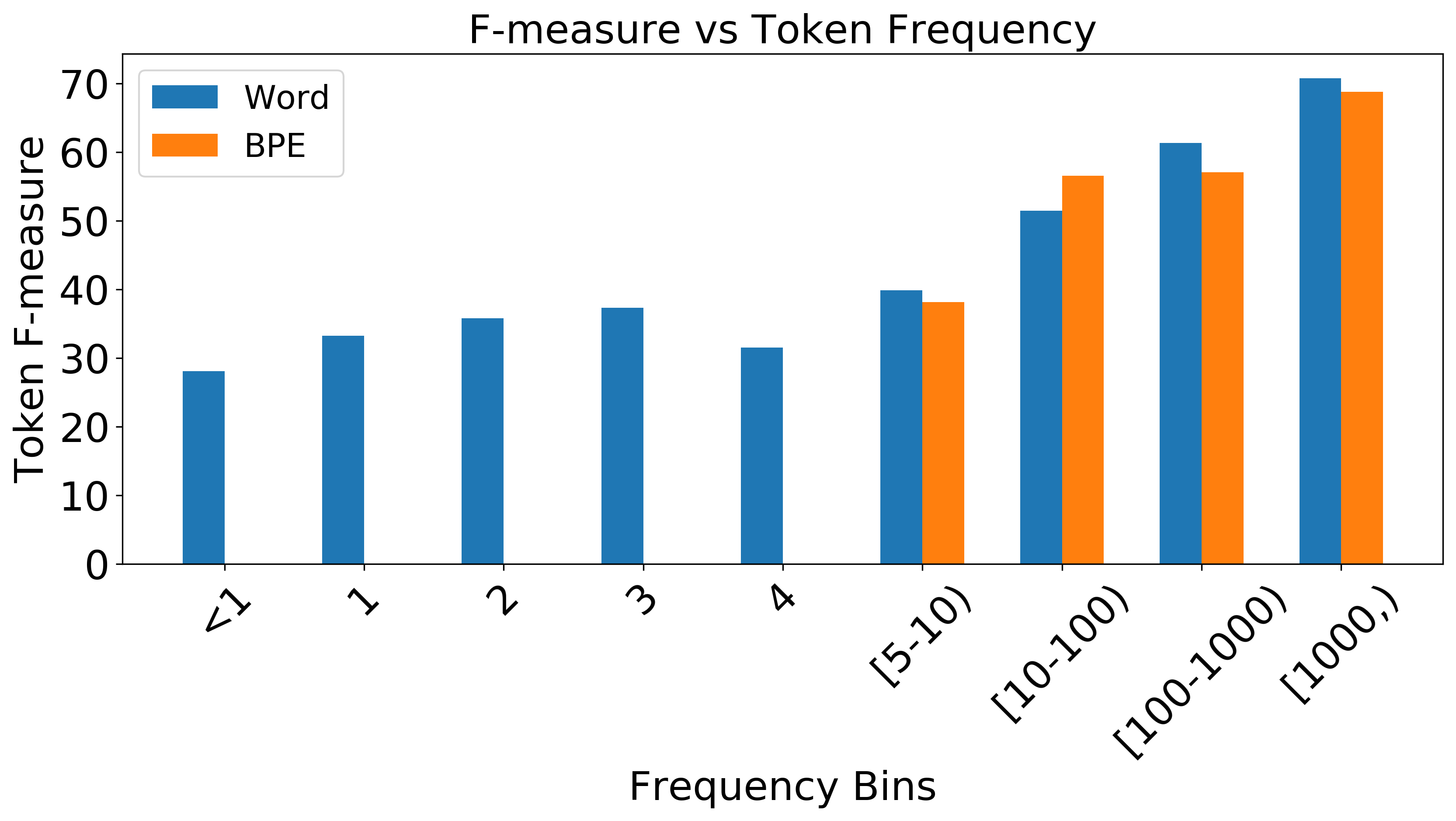
Figure 1: Token F-measure bucketed by Frequency: F-measure correlates with the tokens’ training frequency.

2.1 Token Level

At the token level, Zipf’s law Powers (1998) serves as the primary culprit for the long-tail in word distributions, and consequently, for sub-word (such as BPE Sennrich et al. (2016)) distributions . Figure 1 shows the F-measure Neubig et al. (2019) of the target tokens bucketed by their frequency in the training corpus, as evaluated on the validation set. Clearly, for tokens occurring only a few times, the F-measure is considerably lower for both words and subwords, demonstrating that the model isn’t able to effectively generate low-frequency tokens in the output. Next, we study how this phenomenon is exhibited at the sequence (sentence) level.

2.2 Sequence Level

To quantify the long-tailed phenomena manifesting at the sentence level, we define a simple measure named the Frequency-Score, $F_{S}$ of a sentence, computed simply as the average frequency of the tokens in the sentence. Precisely, for a sequence $x$ comprising of $N$ tokens $[x_{1},\ldots,x_{i},\ldots,x_{N}]$, we define the Frequency-Score $F_{S}$ as: $F_{S}(x)=\cfrac{\sum_{i=1}^{N}f(x_{i})}{N}$, where $f(x_{i})$ is the frequency of the token $x_{i}$ in the training corpus. We compute $F_{S}$ for each source sequence in the IWSLT 2014 De-En validation set, and split it into three parts of $2400$ sentences each, in terms of decreasing $F_{S}$ of the source sequences. The splits are constructed by dividing the validation set into three equal parts based on the Frequency-score, so that we can compare the performance between the three splits for a given model.

Table 1 shows the model performance on the three splits. Scores for 3 widely used MT metrics Clark et al. (2011): BLEU, METEOR and TER as well as the Recall BERT-Score (R-BERT) Zhang et al. (2020) are reported. The arrows represent the direction of better scores. The table shows that model performance across all metrics deteriorates as the mean $F_{S}$ value, $\hat{F_{S}}$ of the split decreases. On aggregate, this demonstrates that the model isn’t able to effectively handle sentences with low $F_{S}$.

Split	$\cfrac{\boldsymbol{\hat{F_{S}}}}{10^{4}}$	BLEU $\uparrow$	METEOR $\uparrow$	TER $\downarrow$	R-BERT $\uparrow$
Highest	7.8	38.6	36.4	41.0	65.2
Medium	5.3	34.1	34.2	45.5	61.0
Least	3.4	33.0	34.1	46.2	60.6

Table 1: Sequence Level Long-Tailed Phenomena: The performance across different metrics deteriorates with the mean Frequency-Score $\hat{F_{S}}$.

3 Related Work

At a high level, we categorize the solutions to better model long-tailed phenomena into three groups, namely, learning better representations, improving (long-tailed) classification and improvements in sequence inference algorithms. In this work, we will be mainly concerned with the interaction between (long-tailed) classification and sequence inference.

Better Representations

Many recent works Qi et al. (2018); Gong et al. (2018); Zhu et al. (2020) propose to either learn better representations for low-frequency tokens or to integrate pre-trained representations into NMT models. To better capture long range semantic structure, Chen et al. (2019) argue for sequence level supervision during learning.

Long-Tailed Classification

A number of works, Lin et al. (2017); Kang et al. (2020), have focused on designing algorithms that improve classification of low-frequency classes. Below, we list two such algorithms, used as baselines in section 5:

Focal Loss

Proposed in Lin et al. (2017), Focal loss (FL) increases the relative loss of low-confidence predictions vis-à-vis high confidence predictions, when compared to cross-entropy. It is described in equation 1, where $\gamma>0$ and $p$ refers to the probability/confidence of the prediction.

$$\vspace{-0.25em}\text{FL}(p)=-(1-p)^{\gamma}\log(p)$$ (1)

$\tau$-Normalization

Kang et al. (2020) link the norms of the penultimate (pre-softmax) layer to the frequency of the class in image classification (also shown to be true in the context of language models Demeter et al. (2020)), and show that normalizing their weights $w_{i}$ i.e. leads to improved classification:

$$\vspace{-0.25em}\tilde{w_{i}}=\cfrac{w_{i}}{\lvert\lvert w_{i}\rvert\rvert^{\tau}}$$ (2)

Here, $\tau$ is a hyperparameter. The intuition behind $\tau$-Normalization is based on the simple observation that the norms of the penultimate layer dictate the feature span of the corresponding class during prediction.

At the sequence level, a parallel line of work has explored penalizing overconfident predictions Meister et al. (2020), e.g., Label smoothing has been shown to yield consistent gains in seq2seq tasks Müller et al. (2019).

Sequence Inference

Vijayakumar et al. (2018); Huang et al. (2017) try to modify beam search to allow for better exploring the output state space.

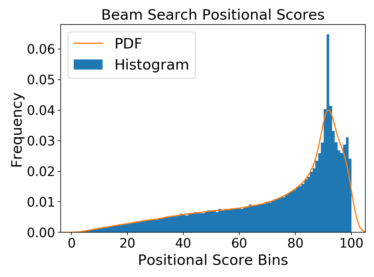
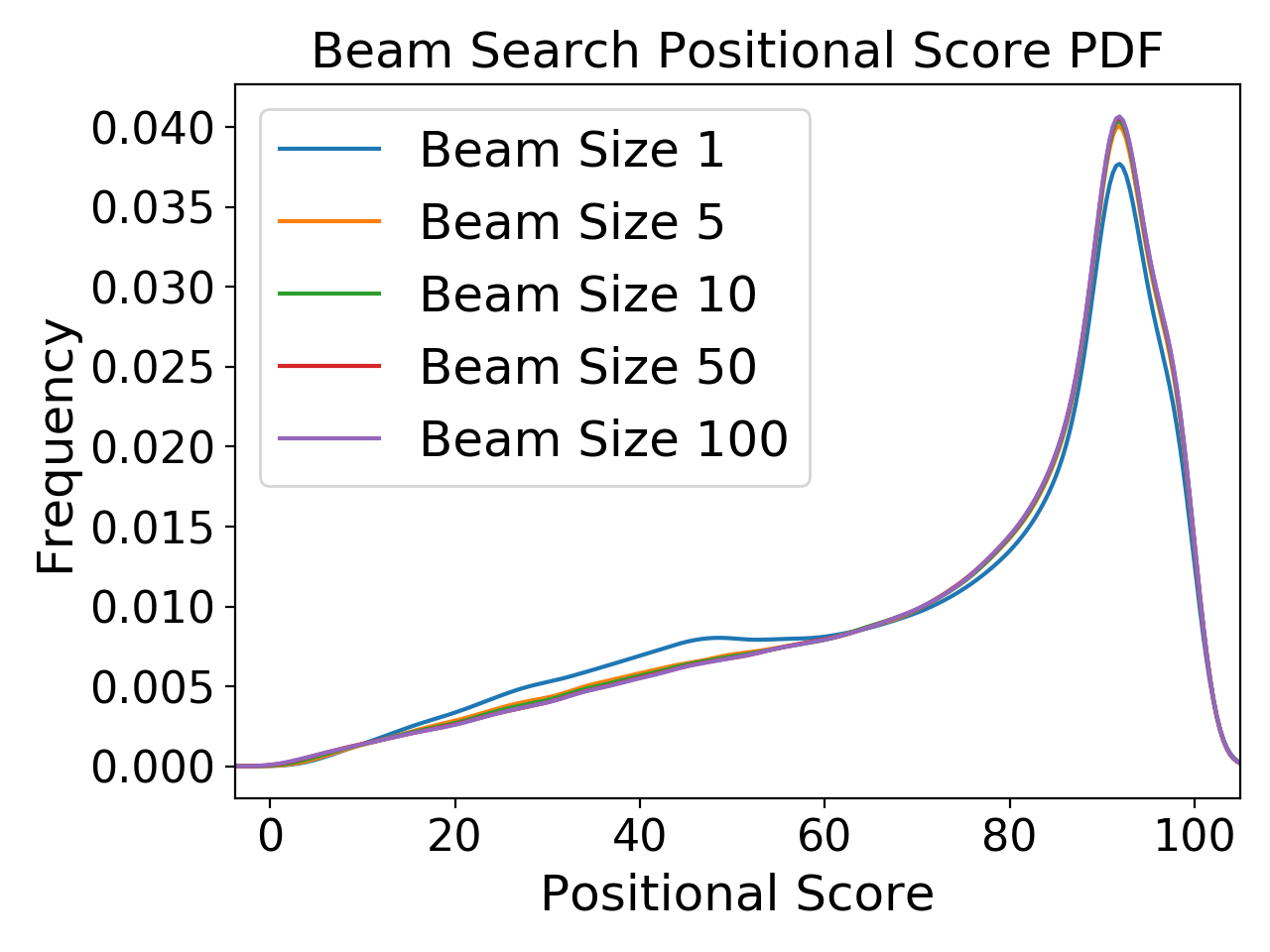
Figure 2: Beam Search Analysis: (Top) Positional scores for Beam size = $5$ and (Bottom) PDFs for different Beam sizes. Scores aggregated over the validation set using the IWSLT 14 De-En Model from section 2.

4 Modeling the Long Tail

To improve the generation of the long-tail of low frequency tokens, it is important to study how low-frequency tokens could appear in the candidate hypotheses during search. Subsequently, we could leverage any such biases from sequence level inference to better model token classification.

Beam Search Analysis To better establish the link between token level classification and beam search inference, we study the distribution of positional scores, i.e. the probabilities selected during each step of decoding, for the top hypothesis finally selected during beam search. The top plot in Figure 2 shows the histogram of the positional scores, aggregated on the validation set. A Gaussian Kernel density estimator is fitted to the histograms as well, and probability density functions (PDFs) for positional scores are plotted for different beam sizes in Figure 2 (the bottom plot).

An analysis of the positional scores (Figure 2, top) reveals that approximately 40 $\%$ of the tokens selected in the top hypothesis have probabilities below 0.75. Further, the bottom plot in Figure 2 shows that this distribution is consistent across different beam sizes. These observations show that the approximate inference procedure of beam-search relies significantly on low confidence predictions. However, if low-confidence predictions are excessively penalized, the conditional probability distribution will be pushed to lower and lower entropy, hurting effective search. Therefore, we argue that a better trade-off between token level classification and sequence level inference in NMT could be established by allowing low-confidence predictions to suffer less penalization vis-à-vis cross-entropy.

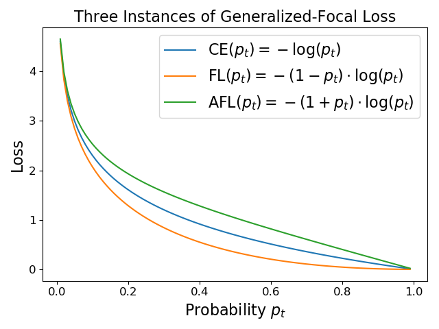
Figure 3: Comparison of the Loss Functions: Focal loss penalizes low-confidence predictions most aggressively, while Anti-Focal loss relaxes the relative loss for low-confidence predictions vis-à-vis cross-entropy.

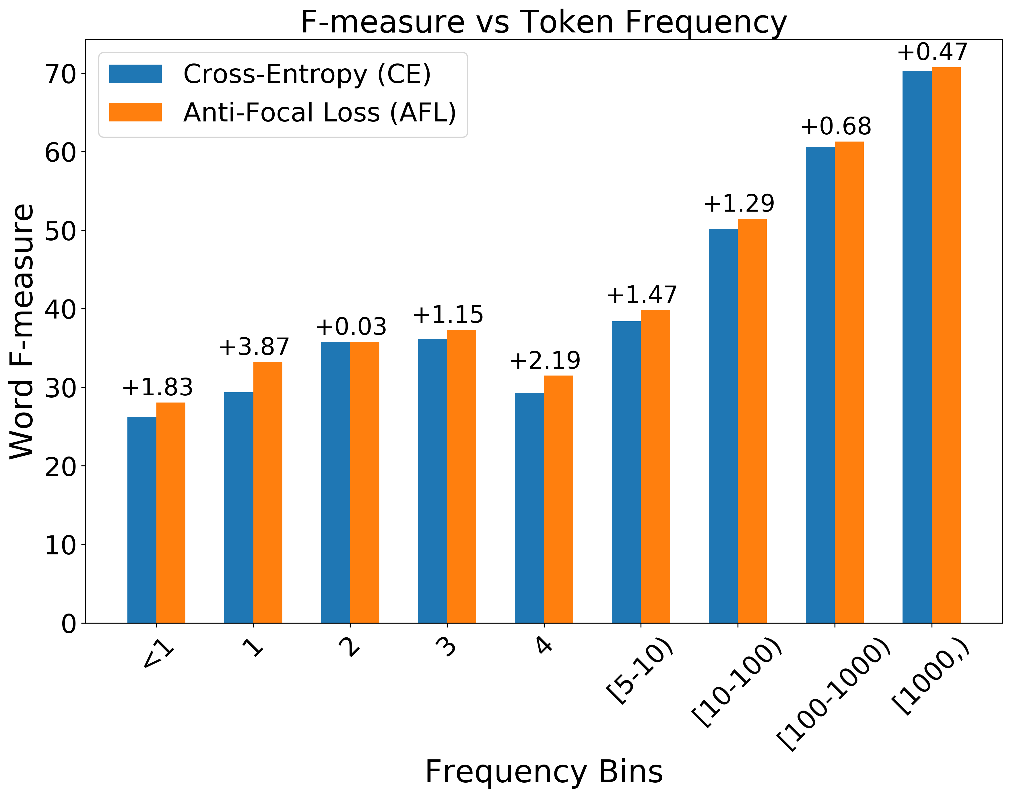
Figure 4: Test Word F-measure bucketed by Training Frequency: AFL leads to gains in F-measure across different frequency bins, especially in low-frequency bins.

			FL		CE + $\tau$-Norm		AFL		AFL + $\tau$-Norm
Dataset	Pair	CE	$\gamma=1$	$\gamma=2$	$\tau=0.2$	$\tau=0.4$	$\alpha=0.5$	$\alpha=1$	$\alpha=1$, $\tau=0.2$
IWSLT 14	De-En	32.15	31.53	30.60	32.62	32.48	32.95	33.17	33.41
IWSLT 14	En-De	26.93	26.27	25.35	27.16	26.69	27.35	27.05	27.31
IWSLT 14	Es-En	38.95	38.30	37.41	39.29	39.28	39.33	39.47	39.86
IWSLT 17	En-Fr	34.40	34.60	32.60	34.30	33.70	35.40	34.90	34.80
IWSLT 17	Fr-En	34.60	34.00	33.30	35.10	34.60	35.00	35.00	35.30
TED Talks	Ru-En	25.22	24.24	23.68	25.22	24.97	25.39	25.64	25.70
TED Talks	Pt-En	34.31	32.78	31.17	34.68	34.56	34.43	35.06	35.31
TED Talks	Gl-En	13.66	13.53	13.26	13.86	13.73	14.82	13.73	13.84
TED Talks	Be-En	03.56	04.01	04.28	03.78	03.92	03.97	04.63	04.69

Table 2: Test BLEU Scores of the Baselines & the Proposed Method. Anti-Focal loss consistently leads to significant gains over cross-entropy, with a $p$-value < $0.01$ for each language pair Clark et al. (2011). Here CE, FL, and AFL represent cross-entropy, focal, Anti-focal loss respectively. Validation results are presented in Appendix C.

Anti-Focal Loss

Now, we try to establish a better trade-off for penalizing low-confidence predictions, which could help improve search, while being simple and automatic. Firstly, we generalize Focal loss by introducing a new term $\alpha$ in equation 1:

$$\vspace{-0.25em}\text{Generalized-FL}(p)=-(1+\alpha\cdot p)^{\gamma}\log(p)\vspace{-0.25em}$$ (3)

Clearly, for $\alpha=-1$ and $\gamma>0$, Generalized-FL (equation 3) reduces to the Focal loss, while for $\alpha=0$, it reduces to the cross-entropy loss. Since we intend to increase the entropy of the conditional token classifier in NMT, we propose to use Generalized-FL with $\alpha>0$ and $\gamma>0$, which we name as Anti-Focal loss (AFL). To understand how AFL realizes the intuition derived through beam search analysis, consider Figure 3. Figure 3 shows the plot for CE, FL with $\gamma=1$ and AFL with $\gamma=1$ and $\alpha=1$. In general, AFL allocates less relative loss to low-confidence predictions. For example, if we compare the relative loss term $\cfrac{loss(p=0.6)}{loss(p=0.9)}$ for the three different losses in Figure 3, then CE has a score of 4.85, FL has a score of 19.39, while AFL has a score of 4.08. Further, using $\alpha$ and $\gamma$, we can manipulate the relative loss. Empirically, we find that $\gamma=1$ and $\alpha\in\{0.5,1.0\}$ works well for AFL in practice.

5 Experiments and Results

We evaluate our proposed Anti-Focal loss against different baselines (CE, FL, $\tau$-Norm) on the task of NMT and analyze the results for further insights.

Datasets and Baselines

We evaluate the proposed algorithm on the widely studied IWSLT 14, IWSLT 17 Cettolo et al. (2017) and the Multilingual TED Talks datasets Qi et al. (2018) (details in Appendix A). For model training, we replicate the hyperparameter settings of Zhu et al. (2020), except that we do not include label-smoothing for a fair comparison of the loss functions (CE, FL, AFL). $\gamma=1$ is set for AFL. Further, $\tau$-Normalization ($\tau$-Norm) was applied post-training both for CE, AFL. Hyperparameters $\gamma,\alpha,\tau$ were manually tuned.

Experimental Settings

For experiments, we use fairseq Ott et al. (2019) (more details in Appendix B). For each language pair, BPE with a joint token vocabulary of 10K was applied over tokenized text. A six-layer Transformer model with embedding size 512, FFN layer dimension 1024 and 4 attention heads (42M parameters), was trained for 50K updates for IWSLT datasets and 40K updates for TED Talks datasets. A batch size of 4K tokens, dropout of 0.3 and tied encoder-decoder embeddings were used. BLEU evaluation (tokenized) for IWSLT 14 and TED talks datasets is done using multi-bleu.perl, while for IWSLT 17 datasets SacreBLEU is used Post (2018). All models were trained on one Nvidia 2080Ti GPU and a beam size of 5 was used for each evaluation.

Results

The trends in Table 2 show that AFL consistently leads to significant gains over cross-entropy. Further, in Table 3 we compare CE and AFL ($\alpha=1$) for the three validation splits created in section 2.2, for the IWSLT 14 De-En dataset. Table 3 shows that AFL improves the model the most on the split with the least $\hat{F_{S}}$, while leading to consistent gains on all the three splits.

Further, Figure 4 shows that AFL also leads to gains in word F-measure across different low-frequency bins (evaluated on the test set), implying better generation of low-frequency words. Here, the analysis was done on semantically meaningful word units, using the generated output after the BPE merge operations. Figure 5 in Appendix D shows that similar trend holds true for BPE tokens as well. Table 2 also shows that $\tau$-Normalization helps improve BLEU for both CE and AFL, except on En-Fr, providing a simple way to improve NMT models. In general, $\tau$-Norm + AFL leads to the best BLEU scores in Table 2.

Discussion.

The results show that AFL ameliorates low-frequency word generation in NMT, leading to improvements for long-tailed phenomena both at the token and sentence level. Further, on the two very low-resource language pairs of Be-En and Gl-En, FL leads to improvements, suggesting that under severely poor conditional modeling i.e token classification, explicitly improving long-tailed token classification helps sequence generation in NMT. However, since FL is more aggressive than CE in pushing low-confidence predictions to higher confidence values, in high-resource pairs (with better token classification), FL ends up hurting beam search. Conversely, AFL achieves significant gains in BLEU scores by incorporating the inductive biases of beam search, e.g. in the comparatively higher-resource IWSLT-17 En-Fr dataset (237K training sentence pairs). Here, we also hypothesize that the long-tailed phenomena have considerably different characteristics for low-resource and high-resource language pairs, but leave further analysis for future work.

Split	Loss	BLEU $\uparrow$	METEOR $\uparrow$	TER $\downarrow$	R-BERT $\uparrow$
Highest	CE	36.7	35.5	41.7	64.0
Highest	AFL	37.1	35.7	41.4	64.3
Medium	CE	32.3	33.3	46.3	59.9
Medium	AFL	33.3	33.6	45.4	60.5
Least	CE	31.3	33.2	46.9	59.7
Least	AFL	32.1	33.5	46.4	60.4

Table 3: Sequence Level Long-Tailed Phenomena: CE vs AFL for different MT metrics, for IWSLT 14 De-En.

6 Conclusion and Future Work

In this work, we characterized the long-tailed phenomena in NMT and demonstrated that NMT models aren’t able to effectively generate low-frequency tokens in the output. We proposed a new loss function, the Anti-Focal loss, to incorporate the inductive biases of beam search into the NMT training process. We conducted comprehensive evaluations on 9 language pairs with different amounts of training data from the IWSLT and TED corpora. Our proposed technique leads to gains across a range of metrics, improving long-tailed NMT at both the token as well as at the sequence level. In future, we wish to explore its connections to entropy regularization and model calibration and whether we can fully encode the inductive biases of label smoothing in the loss function itself.

Appendix A Dataset Statistics

The dataset statistics are highlighted in Table 6, while descriptions of the language pairs are provided in Table 5. The preparation of validation and test sets for IWSLT 14 and 17 datasets is done using fairseq Ott et al. (2019) scripts, following Zhu et al. (2020) for the corresponding datasets. The TED talks dataset is provided with train, validation and test sets Qi et al. (2018). Further, the TED talks dataset is tokenized using moses, and the data preparation script is based on the IWSLT 14 data preparation script in fairseq. We have provided the data preparation scripts as well, from download to pre-processing for each of the datasets, in the code.

			FL		CE + $\tau$-Norm		AFL		AFL + $\tau$-Norm
Dataset	Pair	CE	$\gamma=1$	$\gamma=2$	$\tau=0.2$	$\tau=0.4$	$\alpha=0.5$	$\alpha=1$	$\alpha=1$, $\tau=0.2$
IWSLT 14	De-En	33.44	33.39	33.17	33.86	33.64	33.98	34.34	34.64
IWSLT 14	En-De	28.02	27.22	26.37	27.87	27.20	28.35	28.23	28.27
IWSLT 14	Es-En	41.19	40.36	39.31	41.39	41.08	41.26	41.26	41.65
IWSLT 17	En-Fr	34.60	33.67	33.67	33.98	33.41	34.81	33.93	34.12
IWSLT 17	Fr-En	32.73	32.16	31.89	33.05	32.82	32.56	33.12	33.16
TED Talks	Ru-En	25.50	24.85	24.33	25.65	24.67	25.86	25.88	25.95
TED Talks	Pt-En	35.34	33.42	32.47	35.47	35.09	35.68	35.71	36.05
TED Talks	Be-En	04.24	05.25	05.43	04.54	04.39	05.46	05.35	05.71
TED Talks	Gl-En	14.64	14.66	13.54	14.95	14.87	15.72	15.17	14.97

Table 4: BLEU Scores of the Baselines and the Proposed Method on the Validation set.

Dataset	Source	Target	Lang-Pair
IWSLT 14	German	English	De-En
IWSLT 14	English	German	En-De
IWSLT 14	Spanish	English	Es-En
IWSLT 17	English	French	En-Fr
IWSLT 17	French	English	Fr-En
TED Talks	Russian	English	Ru-En
TED Talks	Portuguese	English	Pt-En
TED Talks	Belarusian	English	Be-En
TED Talks	Galician	English	Gl-En

Table 5: Dataset Language Pair Details: The abbreviations for the language pairs are used throughout.

Dataset	Pairs	Train	Valid	Test
IWSLT 14	En-De	160,239	7,283	6,750
IWSLT 14	De-En	160,239	7,283	6,750
IWSLT 14	Es-En	169,028	7,683	5,593
IWSLT 17	En-Fr	236,652	890	1,210
IWSLT 17	Fr-En	236,652	890	1,210
TED Talks	Ru-En	208,106	4,805	5,476
TED Talks	Pt-En	051,785	1,193	1,803
TED Talks	Gl-En	010,017	0682	1,007
TED Talks	Be-En	004,509	0248	0664

Table 6: Dataset Statistics: Train, Validation and Test Splits for each of the Language Pairs.

Appendix B Model Details

The Transformer model is the iwslt-de-en model architecture in fairseq , also used in Zhu et al. (2020). It is a six-layer Transformer model (6 layers in both the encoder and decoder) with embedding size 512, FFN layer dimension 1024 and 4 attention heads. The optimizer used is Adam, with a learning rate of 0.0005, with 4K warmup updates a warmup initial learning rate of $1e-07$. We have provided training as well as evaluation scripts for each of the datasets in the code. The loss functions are implemented by subclassing cross-entropy in the fairseq framework and are available in the Criterions directory.

Appendix C Validation Results

Table 4 provides the results for the Validation set, corresponding to the test set evaluation done in Table 2 in section 5 of the main paper. The evaluation settings remain the same as in Section 5, except that, the validation results for IWSLT 17 are obtained using multi-bleu.perl instead of SacreBLEU Post (2018). In general, Validation set results also adhere to the same trend as in Section 5. In particular, Anti-Focal, combined with $\tau$-Normalization (AFC + $\tau$-Norm) leads to gains in cross-entropy over each of the datasets.

Appendix D F-Measure Comparison

Figure 5 presents the token-level comparison on the generated output without merging the BPE tokens, i.e. Figure 5 is the BPE token analogue of Figure 4 in Section 5. Here also, we observe similar trend for AFL, i.e. AFL leads to considerable gains in F-measure in the lower frequency buckets (e.g. [5-10)), when compared to cross-entropy.

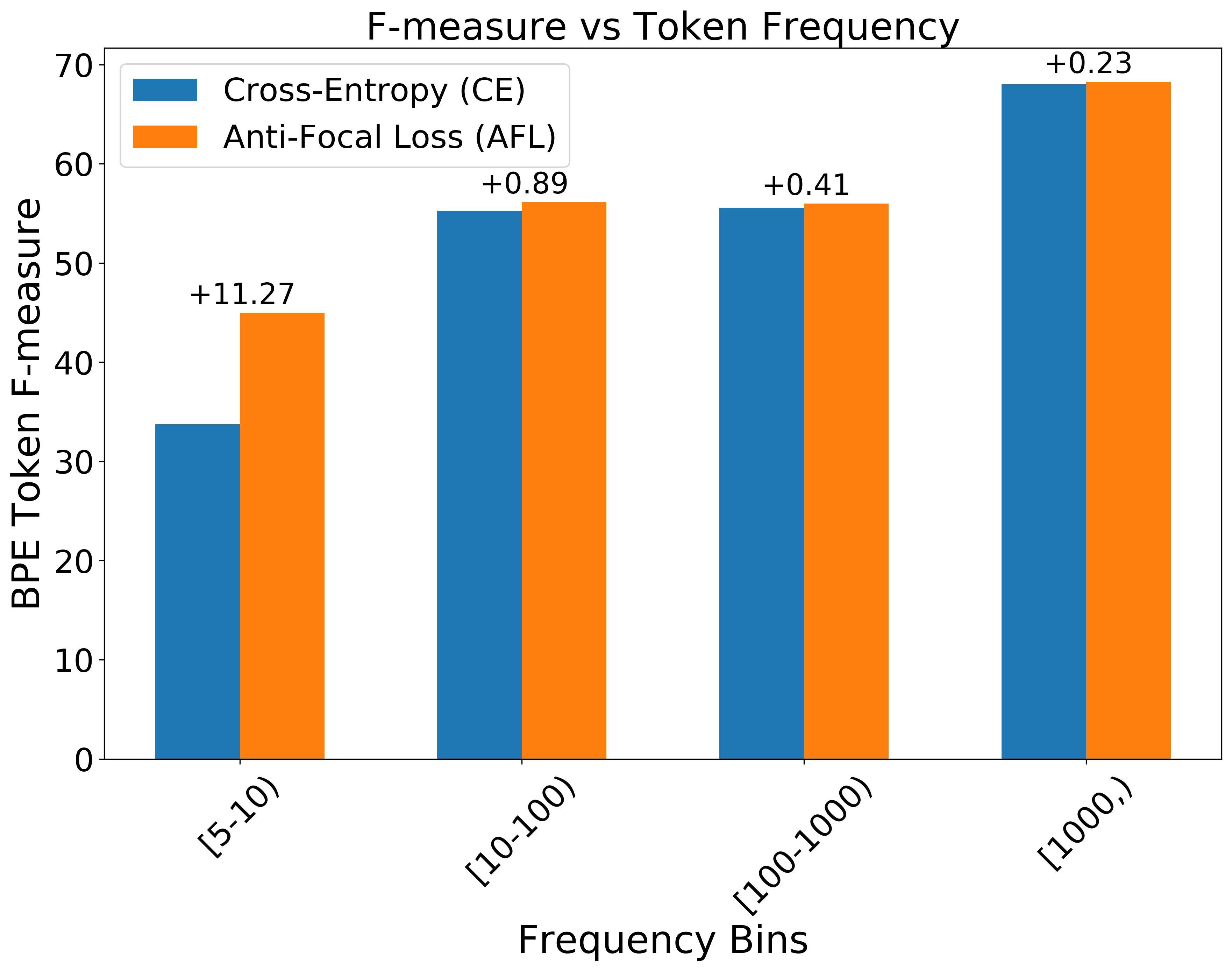
Figure 5: Test F-measure for BPE tokens bucketed by Training Frequency: AFL leads to gains in F-measure across different frequency bins, especially in low-frequency bins.

References

- Cettolo et al. (2017) Mauro Cettolo, Marcello Federico, Luisa Bentivogli, Niehues Jan, Stüker Sebastian, Sudoh Katsuitho, Yoshino Koichiro, and Federmann Christian. 2017. Overview of the IWSLT 2017 evaluation campaign. In International Workshop on Spoken Language Translation, pages 2–14.
- Cettolo et al. (2014) Mauro Cettolo, J Niehues, S Stüker, Luisa Bentivogli, and Marcello Federico. 2014. Report on the 11th IWSLT Evaluation Campaign, IWSLT 2014. In IWSLT-International Workshop on Spoken Language Processing, pages 2–17.
- Chen et al. (2019) Liqun Chen, Yizhe Zhang, Ruiyi Zhang, Chenyang Tao, Zhe Gan, Haichao Zhang, Bai Li, Dinghan Shen, Changyou Chen, and Lawrence Carin. 2019. Improving Sequence-to-Sequence Learning via Optimal Transport. In International Conference on Learning Representations.
- Clark et al. (2011) Jonathan H. Clark, Chris Dyer, Alon Lavie, and Noah A. Smith. 2011. Better Hypothesis Testing for Statistical Machine Translation: Controlling for Optimizer Instability. In Proceedings of the 49th Annual Meeting of the Association for Computational Linguistics: Human Language Technologies, pages 176–181, Portland, Oregon, USA. Association for Computational Linguistics.
- Demeter et al. (2020) David Demeter, Gregory Kimmel, and Doug Downey. 2020. Stolen Probability: A Structural Weakness of Neural Language Models. In Proceedings of the 58th Annual Meeting of the Association for Computational Linguistics, pages 2191–2197, Online. Association for Computational Linguistics.
- Gong et al. (2018) Chengyue Gong, Di He, Xu Tan, Tao Qin, Liwei Wang, and Tie-Yan Liu. 2018. FRAGE: Frequency-Agnostic Word Representation. In Advances in Neural Information Processing Systems 31, pages 1334–1345.
- Huang et al. (2017) Liang Huang, Kai Zhao, and Mingbo Ma. 2017. When to Finish? Optimal Beam Search for Neural Text Generation (modulo beam size). In Proceedings of the 2017 Conference on Empirical Methods in Natural Language Processing, pages 2134–2139, Copenhagen, Denmark. Association for Computational Linguistics.
- Kang et al. (2020) Bingyi Kang, Saining Xie, Marcus Rohrbach, Zhicheng Yan, Albert Gordo, Jiashi Feng, and Yannis Kalantidis. 2020. Decoupling Representation and Classifier for Long-Tailed Recognition. In International Conference on Learning Representations.
- Lake and Baroni (2018) Brenden M. Lake and Marco Baroni. 2018. Generalization without Systematicity: On the Compositional Skills of Sequence-to-Sequence Recurrent Networks. In Proceedings of the 35th International Conference on Machine Learning, ICML 2018, Stockholm, Sweden, volume 80 of Proceedings of Machine Learning Research, pages 2879–2888. PMLR.
- Lin et al. (2017) Tsung-Yi Lin, Priya Goyal, Ross Girshick, Kaiming He, and Piotr Dollár. 2017. Focal loss for dense object detection. In Proceedings of the IEEE international conference on computer vision, pages 2980–2988.
- Meister et al. (2020) Clara Meister, Elizabeth Salesky, and Ryan Cotterell. 2020. Generalized Entropy Regularization or: There’s Nothing Special about Label Smoothing. In Proceedings of the 58th Annual Meeting of the Association for Computational Linguistics, pages 6870–6886, Online. Association for Computational Linguistics.
- Müller et al. (2019) Rafael Müller, Simon Kornblith, and Geoffrey E Hinton. 2019. When does label smoothing help? In Advances in Neural Information Processing Systems 32, pages 4694–4703.
- Murray and Chiang (2018) Kenton Murray and David Chiang. 2018. Correcting Length Bias in Neural Machine Translation. In Proceedings of the Third Conference on Machine Translation: Research Papers, pages 212–223, Brussels, Belgium. Association for Computational Linguistics.
- Neubig et al. (2019) Graham Neubig, Zi-Yi Dou, Junjie Hu, Paul Michel, Danish Pruthi, and Xinyi Wang. 2019. compare-mt: A Tool for Holistic Comparison of Language Generation Systems. In Proceedings of the 2019 Conference of the North American Chapter of the Association for Computational Linguistics (Demonstrations), pages 35–41, Minneapolis, Minnesota. Association for Computational Linguistics.
- Ott et al. (2019) Myle Ott, Sergey Edunov, Alexei Baevski, Angela Fan, Sam Gross, Nathan Ng, David Grangier, and Michael Auli. 2019. fairseq: A Fast, Extensible Toolkit for Sequence Modeling. In Proceedings of the 2019 Conference of the North American Chapter of the Association for Computational Linguistics (Demonstrations), pages 48–53, Minneapolis, Minnesota. Association for Computational Linguistics.
- Post (2018) Matt Post. 2018. A Call for Clarity in Reporting BLEU Scores. In Proceedings of the Third Conference on Machine Translation: Research Papers, pages 186–191, Brussels, Belgium. Association for Computational Linguistics.
- Pouget-Abadie et al. (2014) Jean Pouget-Abadie, Dzmitry Bahdanau, Bart van Merriënboer, Kyunghyun Cho, and Yoshua Bengio. 2014. Overcoming the Curse of Sentence Length for Neural Machine Translation using Automatic Segmentation. In Proceedings of SSST-8, Eighth Workshop on Syntax, Semantics and Structure in Statistical Translation, pages 78–85, Doha, Qatar. Association for Computational Linguistics.
- Powers (1998) David M. W. Powers. 1998. Applications and Explanations of Zipf’s Law. In New Methods in Language Processing and Computational Natural Language Learning.
- Qi et al. (2018) Ye Qi, Devendra Sachan, Matthieu Felix, Sarguna Padmanabhan, and Graham Neubig. 2018. When and Why Are Pre-Trained Word Embeddings Useful for Neural Machine Translation? In Proceedings of the 2018 Conference of the North American Chapter of the Association for Computational Linguistics: Human Language Technologies, Volume 2 (Short Papers), pages 529–535, New Orleans, Louisiana. Association for Computational Linguistics.
- Raunak et al. (2019) Vikas Raunak, Vaibhav Kumar, and Florian Metze. 2019. On compositionality in neural machine translation. NeurIPS Workshop, Context and Compositionality in Biological and Artificial Neural Systems.
- Reddy (1988) Raj Reddy. 1988. Foundations and Grand Challenges of Artificial Intelligence: AAAI Presidential Address. AI Magazine, 9(4):9–9.
- Sennrich et al. (2016) Rico Sennrich, Barry Haddow, and Alexandra Birch. 2016. Neural Machine Translation of Rare Words with Subword Units. In Proceedings of the 54th Annual Meeting of the Association for Computational Linguistics (Volume 1: Long Papers), pages 1715–1725, Berlin, Germany. Association for Computational Linguistics.
- Vaswani et al. (2017) Ashish Vaswani, Noam Shazeer, Niki Parmar, Jakob Uszkoreit, Llion Jones, Aidan N Gomez, Ł ukasz Kaiser, and Illia Polosukhin. 2017. Attention is All you Need. In Advances in Neural Information Processing Systems 30, pages 5998–6008.
- Vijayakumar et al. (2018) Ashwin K Vijayakumar, Michael Cogswell, Ramprasaath R Selvaraju, Qing Sun, Stefan Lee, David Crandall, and Dhruv Batra. 2018. Diverse beam search: Decoding diverse solutions from neural sequence models. In Thirty-Second AAAI Conference on Artificial Intelligence.
- Zhang et al. (2020) Tianyi Zhang, Varsha Kishore, Felix Wu, Kilian Q. Weinberger, and Yoav Artzi. 2020. BERTScore: Evaluating Text Generation with BERT. In International Conference on Learning Representations.
- Zhao and Marcus (2012) Qiuye Zhao and Mitch Marcus. 2012. Long-Tail Distributions and Unsupervised Learning of Morphology. In Proceedings of COLING 2012, pages 3121–3136, Mumbai, India. The COLING 2012 Organizing Committee.
- Zhu et al. (2020) Jinhua Zhu, Yingce Xia, Lijun Wu, Di He, Tao Qin, Wengang Zhou, Houqiang Li, and Tie-Yan Liu. 2020. Incorporating BERT into Neural Machine Translation. In International Conference on Learning Representations.