Lindblad equation approach to the determination of the optimal working point in nonequilibrium stationary states of an interacting electronic one-dimensional system: Application to the spinless Hubbard chain in the clean and in the weakly disordered limit

Abstract

Using the Lindblad equation approach, we derive the range of the parameters of an interacting one-dimensional electronic chain connected to two reservoirs in the large bias limit in which an optimal working point (corresponding to a change in the monotonicity of the stationary current as a function of the applied bias) emerges in the nonequilibrium stationary state.

In the specific case of the one-dimensional spinless fermionic Hubbard chain, we prove that an optimal working point emerges in the dependence of the stationary current on the coupling between the chain and the reservoirs, both in the interacting and in the noninteracting case.

We show that the optimal working point is robust against localized defects of the chain, as well as against a limited amount of quenched disorder.

Eventually, we discuss the importance of our results for optimizing the performance of a quantum circuit by tuning its components as close as possible to their optimal working point.

I Introduction

Connecting a mesoscopic device with two or more electronic reservoirs, biased at different temperatures or chemical potentials, gives rise to finite currents flowing through the system, between the reservoirs. At a low bias, the (equilibrium) transport properties of the system are well accounted for, both analytically and numerically, within linear response approach Mello and Kumar (2004). Conversely, when the system is driven to the nonequilibrium regime (large bias), a fully analytical approach is in practice unfeasible, due to the strong dependence of the dynamics on the system and on the reservoirs separately, as well as on the nature of the coupling between the two of them Prosen (2008).

Despite the technical difficulties to approach it, the large bias regime is of great interest, as it is directly related to, e.g., control of heat flow Henrich et al. (2007), as well as quantum information processing Burgarth and Giovannetti (2007). For this reason, a large number of theoretical approaches has been developed to investigate the nature of nonequilibrium states, both in noninteracting, as well as in interacting systems, such as the Landauer-Buttiker formalism You et al. (2000); Datta (1993), the quantum master equation approach Gorini et al. (1976); Lindblad (1976), the renormalization group techniques Schoeller (2009); Berges and Mesterházy (2012) (including the functional renormalization group approach Jakobs et al. (2007)), and the bosonization methods Gutman et al. (2010); Ngo Dinh et al. (2012); Levkivskyi (2012). Yet, each of these methods has only a limited range of applicability and, typically, none of them is able to fully catch all the relevant aspects of nonequilibrium physics, due to the complexity of the systems, to the strength of the interaction, to the peculiar nature of the stationary states that eventually set in, et cetera.

Therefore, to fully recover the nonequilibrium physics, one has to resort to a fully numerical approach, possibly complemented, when possible, with (approximate) analytical methods. In fact, when connected to one, or more, reservoirs, (open) quantum systems can be described through a master equation, aimed to represent the true quantum evolution after integrating over the reservoir degrees of freedom. The derivation of such equation usually relies on the so-called Markovian approximation, which consists of neglecting memory effects under the assumption that the bath relaxation time is much shorter than the characteristic timescales of the system Breuer and Petruccione (2002); Weiss (1993). The Lindblad equation (LE) Lindblad (1976) is among the most used master equations: it stems from modeling the reservoirs as local “jump” operators injecting, or removing, particles through the boundaries of the system. Aside of its universality, the LE can be readily approached by means of a number of numerical methods, including Quantum Monte Carlo techniques Carlo et al. (2003, 2004); Benenti et al. (2009a), time-dependent density matrix renormalization group ($t$-DMRG) Vidal (2003, 2004); White and Feiguin (2004); Brenes et al. (2018) or current density functional approach Langer et al. (2009).

Most of the literature concerning the numerical approach to the LE has been focused onto quantum $XXZ$ spin chains connected to reservoirs. The $XXZ$ spin-1/2 spin chain, indeed, provides a remarkable paradigmatic model where to address several key issues, such as the interplay between integrability breaking and asymptotic evolution of the system towards an appropriate nonequilibrium stationary state (NESS) Benenti et al. (2009b), the characterization of the NESS by looking at the real-space average magnetization in the $z$-direction and at the stationary spin current flowing through the chain, the effects of isolated impurities as well as of quenched disorder on the NESS Brenes et al. (2018); Sabetta and Misguich (2013), and so on. In addition, the quantum $XXZ$ spin chain is well-known to map onto a model for spinless interacting one-dimensional lattice fermions (which throughout the paper we dub “spinless fermionic Hubbard model” (1HM), according to the widely used terminology Sznajd and Becker (2005); Thomaz et al. (2014)), via Jordan-Wigner transformation Jordan and Wigner (1928). Finally, it has been shown that it is possible to realize quantum spin-1/2 $XXZ$ spin chains with tunable impurities at pertinently engineered junctions of one-dimensional Josephson junction arrays Giuliano and Sodano (2005, 2008, 2009); Cirillo et al. (2011).

A typical feature characterizing the NESS in the $XXZ$ spin-1/2 spin chain is the tendency of the system, driven out of equilibrium, to develop ferromagnetic domains, separated by domain walls that conspire to reduce the spin-flip rate and, therefore, to reduce the nonequilibrium stationary spin current through the chain Benenti et al. (2009b); Karevski and Platini (2009). Similarly, the NESS in the 1HM is characterized by the emergence of domains in the chain with a uniform charge distributions, separated by charge domain walls that generate a counterfield reducing the total current $I_{\rm st}$ flowing across the system in the NESS. The domain walls give rise, at large enough bias between the reservoirs, to a remarkable negative differential conductance (NDC), that is, to a region in which the current decreases if the bias increases. The NDC is a feature of mesoscopic systems, such as semiconductor superlattices Esaki and Tsu (1970), interacting quantum gases Labouvie et al. (2015), single molecule junctions Perrin et al. (2013), carbon nanotubes Pop et al. (2005), graphene transistors Britnell et al. (2013), and quantum dots coupled to electrodes Thielmann et al. (2005). Also, it can arise as an effect of electron-phonon coupling Zazunov et al. (2006). In a quantum chain driven out of equilibrium the NDC emerges as a combined effect of the coherent many-body correlations and the incoherent charge pumping in the chain from the reservoirs Benenti et al. (2009b).

In general, quantum transport properties in many-body systems strongly depend on the interplay between bulk hopping processes, electron-electron interaction, noise and impurity distribution, and boundary driving strength Nazarov and Blanter (2009); Barontini et al. (2013); Ortega et al. (2016). Typically, at small bias, the current induced in the system exhibits Ohmic law behavior, linearly increasing with increasing applied bias. The change in the monotonicity of $I_{\rm st}$ as a function of the applied bias necessarily implies the existence of an ”optimal working point“ (OWP), at which $I_{\rm st}$ takes the maximum value, given the other system parameters. In the 1HM the dependence of the OWP on the interaction has been extensively discussed in Ref.[Benenti et al., 2009a] (a similar analysis in the $XXZ$ chain has been performed in Ref.[Benenti et al., 2009b]). It has been found that, if the coupling strengths between the reservoirs and the 1HM are fixed, a necessary condition to recover the OWP is having a nonzero interaction between the electrons. More generally, making a quantum system that is part of a quantum circuit work at the OWP, means maximizing the current flow supported by that part of the circuit at a given bias. Identifying the OWP for each component of the circuit is a necessary preliminary step to eventually make the circuit operate at its maximum possible efficiency. Moreover, an analogous optimization procedure for, e.g., the energy transport would have striking consequences for optimizing the control of the energy transfer between different part of mesoscopic devices. In addition, the OWP can be associated with nontrivial effects like the tendency to enhance nonuniformities Conwell (1967); Xu and Teitsworth (2007); Cross and Greenside (2009) or the Gunn effect Knight and Peterson (1966, 1967); Qi et al. (2006). Finally, it is worth noticing how the emergence of the OWP is a typical behavior found in fundamental traffic flow diagrams Nagatani (2002, 1998), where the free flow phase and the congested phase are separated by an optimal value of the density, at which the traffic flow (the “current”) is maximum. In fact, this observation would suggest that a quantum chain (or a network) at large bias might potentially work as a “quantum simulator” of the fundamental traffic flow diagram, with potentially countless applications to real-life problems. Therefore, characterizing the OWP and its emergence as a function of the system parameters is of the utmost importance for the implementations of controlled quantum circuits Pamplin (1970); Japaridze et al. (2009); Deng et al. (2000); Chiesa et al. (2019); Asadian et al. (2013). It is, therefore, crucial to extend the analysis of Ref.[Benenti et al., 2009a] to a larger manifold in parameter space, which should possibly include parameters such as the coupling strengths between the reservoirs and the 1HM, the amount of disorder in the system, and so on.

In this paper we systematically analyze the emergence and the characteristics of the OWP in the current $I_{\rm st}$ in the NESS in interacting one-dimensional electronic systems connected to reservoirs, in the large bias limit. Complementing and extending the analysis of Ref.[Benenti et al., 2009a], we search for the OWP by considering how $I_{\rm st}$ changes as a function of the coupling strengths between the reservoirs and the electronic system. To drive the system toward the NESS, we implement the Lindblad master equation for a graph of $N$-sites connected with two, or more reservoirs. In particular, we treat the interaction within mean field (MF) approximation. Verifying, when possible, the consistency of our results with the one already present in the literature, we check that, while allowing us for considerably simplifying the calculations, our method enables us to catch all the fundamental features characterizing the NESS, such as the dependence of $I_{\rm st}$ on the system parameters and the stationary distribution of the particle density in real space.

Specifically, after presenting our approach in the general case of an interacting electronic system defined on a graph connected to an arbitrary number of reservoirs, we address the case study of a 1HM in the large bias limit, first with homogeneous system parameters, then adding a single (“site”- or “bond”-) impurity to the chain, and eventually in the presence of a finite amount of quenched disorder in the system. In all the cases we focus on, we characterize the NESS in terms of the dependence of $I_{\rm st}$ on the coupling strengths between the reservoirs and the electronic system, and of the stationary distribution of the particle density in real space. Doing so, we show that, as a function of the tuning parameters, the OWP emerges at the NESS even in the absence of electronic interaction. Moreover, we directly check that, in the noninteracting, as well as in the interacting case, the OWP is pretty robust against defects in the chain (isolated impurities), as well as against a moderate amount of quenched disorder. Independently tuning the interaction strength and the amount of disorder, we construct the phase diagram of the system in the disorder - interaction strength parameter space and, in particular, we draw the transition region beyond which the OWP disappears, $I_{\rm st}$ becomes zero and the whole system undergoes a Griffiths-like transition from a conducting to an insulating phase. Eventually, we check that our phase diagram is consistent with the one derived in Ref.[Brenes et al., 2018].

Besides characterizing the NESS and the emergence of the OWP, taking advantage of the simplicity and of the effectiveness of our method, we can follow the evolution in time of our system toward the NESS, with no need for running long lasting numerical simulations. This allows us to map out, in various cases of interest, the details of how the 1HM evolves toward the NESS in real time. In particular, doing so we argue how the NESS is largely independent of the state we begin with and, in this respect, how it is a “universal” property of the chain-plus-reservoir system. Also, we indirectly address the interplay between the integrability and the evolution of the system toward the NESS. In general, the conservation laws associated to the integrability Fioravanti and Rossi (2003a, b, 2005) are known to prevent the system from thermalizing toward a state characterized by a macroscopic hydrodynamical behavior in its transport properties Zotos et al. (1997); Benenti et al. (2013). Breaking the integrability by adding a local impurity term to the otherwise integrable Hamiltonian should definitely trigger an evolution toward a well defined NESS Rigol (2009). Yet, we directly verify that the evolution and the NESS itself barely depend on whether the chain is homogeneous, or with an isolated impurity. This highlights how coupling the chain to the reservoirs already breaks the integrability, thus letting the system evolve toward the NESS and, therefore, how, in this specific case, adding an additional impurity to the chain has very little effect, if none at all, on the time evolution toward the NESS and on the NESS itself.

The paper is organized as follows:

• In Section II we present the model Hamiltonian for an interacting electronic system defined over a generic graph. We therefore discuss our MF approach to the electronic interaction, apply it to the graph system Hamiltonian and derive the corresponding LE. Eventually, we write down the conditions defining the NESS and explicitly solve them in the absence of interaction.

• In Section III we present a specific application of our approach to a noninteracting electronic chain connected to two reservoirs at its endpoints. By sampling $I_{\rm st}$ and the charge density distribution from the equilibrium to the large bias limit, as well as by varying the strength of the coupling between the chain and the reservoirs, we show that an OWP emerges, even in the absence of interaction, when considering $I_{\rm st}$, as a function of the coupling strength, taken in the large bias limit.

• In Section IV we extend the analysis of Section III to the 1HM connected to two reservoirs at the endpoints of the chain, at a generic value of the electronic interaction. Doing so, we evidence the rich set of phases generated in the system by turning on the interaction, by particularly focusing on the conductor to insulator phase transition that emerges, in the large bias limit, at strong enough values of the interaction itself, and on its effects on the OWP.

• In Section V we analyze how adding an impurity term to the homogeneous 1HM Hamiltonian affects, in the large bias limit, the evolution of the system toward the NESS and the NESS itself. Specifically, we focus onto two different types of impurities: a “site” impurity, realized by altering on a single site the otherwise uniform chemical potential, and a “bond” impurity, realized by changing the electronic hopping strength of a single bond of the chain.

• In Section VI we analyze the effects of a finite density of impurities (quenched disorder) in the 1HM by systematically discussing the phase diagram of the system, in the large bias limit, in the disorder strength - interaction space, and how the NESS and the OWP are affected by the simultaneous presence of a finite disorder strength and of a nonzero electronic interaction.

• In Section VII we summarize our results and discuss possible further perspectives of our work.

• In Appendix A we present a simple variational calculation that, despite its simplicity, is able to qualitatively catch the main features of the NESS that emerges in the chain in the large bias limit, both in the homogeneous case and in presence of a single site impurity.

II Model Hamiltonian and Lindblad equation

As a model Hamiltonian for a system of spinless, interacting electrons over an $N$-site graph, we use $H$, given by

$$H=-\sum_{j\neq k=1}^{N}J_{j,k}c_{j}^{\dagger}c_{k}-\sum_{j=0}^{N}\mu_{j}c_{j}^{\dagger}c_{j}+\sum_{j\neq k=1}^{N}U_{j,k}n_{j}n_{k}\>\>\>\>.$$ (1)

In Eq.(1), $c_{j},c_{j}^{\dagger}$ are respectively the single-fermion creation and annihilation operator at lattice site $j$, satisfying the canonical anticommutation relations $\left\{c_{j},c_{j^{\prime}}^{\dagger}\right\}=\delta_{j,j^{\prime}}$. $n_{j}=c_{j}^{\dagger}c_{j}$ is the fermion number operator at site $j$. $J_{j,k}$ is the single-fermion hopping strength between sites $j$ and $k$, $\mu_{j}$ is the chemical potential at site $j$, $U_{j,k}$ is the density-density interaction strength between sites $j$ and $k$. Eq.(1) comprises the most general spinless Hubbard-like Hamiltonian for lattice spinless fermions (see, e.g., Ref.[Essler et al., 2005] for a comprehensive review about the one-dimensional Hubbard model). In principle, we allow any site of the lattice to be connected to an external reservoir. In Fig.1a), we provide a sketch of the corresponding graph, with the blue dots representing generic sites and the red dots sites connected to the external reservoirs, as well as to other sites of the graph. A straight line connecting two sites represents a nonzero hopping strength and/or a nonzero interaction strength between the two sites. Following the same drawing code, in Fig.1b) we show the simple graph representing the system on which we focus most of the discussion of the following Sections: a linear chain connected to two reservoirs at its endpoints.

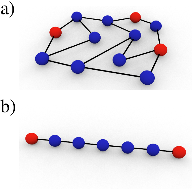
Figure 1:
a): Sketch of a generic graph described by the Hamiltonian $H$ in Eq.(1): the blue dots represent generic sites connected to “internal” sites only, while the red dots represent sites connected to the external reservoirs, as well. A straight line connecting two sites represents a nonzero hopping strength and/or a nonzero interaction strength between the two sites;
b): The special graph we discuss in detail in our paper: a linear chain connected to two reservoirs at its endpoints through two red dots.

To describe the dynamics of the system represented by $H$ in Eq.(1), once it is connected to the external reservoirs, we resort to the master equation (ME) approach to open quantum systems Lindblad (1976); Pearle (2012). Within the ME equaton framework, we derive the effective dynamics of the system by integrating over the reservoir degrees of freedom. Doing so, we resort to the so-called Markovian approximation, consisting in neglecting memory effects under the assumption that the bath relaxation time is much shorter than the characteristic timescales of the system Breuer and Petruccione (2002); Weiss (1993). Eventually, we derive the LE for the open system connected to the reservoirs. The LE is among the most used master equations Adler (2000); Müller and Stace (2017); Nava and Fabrizio (2019); Bácsi et al. (2020): its general form consists of a first order differential equation for the time evolution of the system density matrix $\rho(t)$, given by

$$\dot{\rho}(t)=-i[H,\rho(t)]+\sum_{k}(L_{k}\rho(t)L_{k}^{\dagger}-\frac{1}{2}\{L_{k}^{\dagger}L_{k},\rho(t)\})\>\>\>\>.$$ (2)

The first term at the right-hand side of Eq.(2) is the so-called Liouvillian that describes the unitary evolution determined by $H$. The second term, the so-called Lindbladian, includes dissipation and decoherence on the system dynamics. It depends on the so-called “jump” operators $L_{k}$, which are determined by the coupling between the system and the reservoirs. Specifically, the Liouvillian describes the unitary evolution brought by $H$, while the Lindbladian includes the dissipation and the decoherence in the dynamics.

In the following, we consider reservoirs that locally inject to, or extract fermions from a generic site $j$ of the lattice, at given and fixed rates. Consistently, we describe the injecting and extracting reservoirs at site $j$ in terms of the Lindblad operators $L_{in,j}$ and $L_{out,j}$, given by

$$L_{in,j} = \sqrt{\Gamma_{j}}c_{j}^{\dagger}$$

$$L_{out,j} = \sqrt{\gamma_{j}}c_{j}\>\>\>\>,$$ (3)

with $\Gamma_{j}$ and $\gamma_{j}$ being the coupling strengths respectively determining the creation and the annihilation of a fermion at site $j$.

Once we determine $\rho(t)$ by solving Eq.(2), we compute the (time dependent) expectation value of any observable $O$, $O(t)$ using

$$O(t)={\rm Tr}[O\rho\left(t\right)]\>\>\>\>.$$ (4)

Taking into account Eq.(4) and using the identities

$$\left[A,BC\right] = B\left[A,C\right]+\left[A,B\right]C$$

$$\left[A,BC\right] = \left\{A,B\right\}C-B\left\{A,C\right\}$$

$${\rm Tr}\left(\left[A,B\right]\right) = 0\;\;\;\;,$$ (5)

with $A,B,C$ being operators acting over the same Hilbert space, we employ Eq.(2) to write down the ME directly for $O(t)$. Specifically, we obtain

$$\frac{d}{dt}O(t) = {\rm Tr}(O\dot{\rho}(t))=i{\rm Tr}[[H,O]\rho(t)]$$

$$+ \sum_{k}({\rm Tr}[L_{k}^{\dagger}OL_{k}\rho(t)]-\frac{1}{2}{\rm Tr}[\{L_{k}^{\dagger}L_{k},O\}\rho(t)])\>\>\>\>.$$

For the sake of our analysis, in the following we will need to compute the average value of the occupation number for a generic site $j$ of the system, $n_{j}(t)={\rm Tr}[n_{j}\rho(t)]$, as well as of the currents flowing from the reservoirs into the site $j$, $I_{in,j}(t)$, or from site $j$ to the reservoir, $I_{out,j}(t)$. These are given by

$$I_{in,j}(t) = \Gamma_{i}(1-n_{j}(t))$$

$$I_{out,j}(t) = \gamma_{i}n_{j}(t)\>\>\>\>,$$ (7)

so that the net current exchanged at time $t$ between the reservoirs and the site $j$ is given by $I_{j}(t)=I_{in,j}(t)-I_{out,j}(t)$. In addition, we also need to derive the average value of the current flowing between two connected sites of the graph, say $j$ and $k$, $I_{j,k}$. This is given by

$$I_{j,k}(t)=-iJ_{j,k}{\cal I}_{j,k}(t)+{\rm c.c.}\>\;\;\;,$$ (8)

with ${\cal I}_{j,k}(t)={\rm Tr}[c_{j}^{\dagger}c_{k}\rho(t)]$ and with ${\rm c.c.}$ denoting the complex conjugate.

In principle, solving the full set of Lindblad equations for $n_{j}(t)$, $I_{in,j}(t)$, $I_{out,j}(t)$, and $I_{j,k}(t)$ would allow us to recover the full current pattern over a generic $N$-site graph connected to external reservoirs. However, on increasing $N$, solving the Lindblad equations, even numerically, becomes soon a pretty formidable task to achieve. Indeed, we should solve a hierarchical set of equations in which the expectation values of any combination of $N$ creation and annihilation operators depends on the expectation values of combinations of $N$+2 creation and annihilation operators. In order to exactly describe the system dynamics we should in principle compute the evolution of all the matrix elements of the density matrix, whose dimension is $2^{N}$. Apparently, this becomes soon a hardly accomplishable task, even resorting to a fully numerical approach. For this reason, in the following we resort to a MF approximation, by replacing any occurrence of four-fermion operators with the corresponding approximated expression derived by means of a pertinent Hartree-Fock MF decoupling. Eventually, we check the consistency of our method with a fully numerical approach Benenti et al. (2009a) by comparing the corresponding results in small-size (i.e., $L\leq 16$) systems. In particular, we set

$$n_{j}n_{k} \approx n_{j}(t)n_{k}+n_{k}(t)n_{j}$$ (9)

$$- {\cal I}_{j,k}(t)c_{k}^{\dagger}c_{j}-{\cal I}_{k,j}(t)c_{j}^{\dagger}c_{k}\>\>\>\>.$$

with the first two contributions at the right-hand side of Eq.(9) corresponding to the Hartree terms, the second two contributions to the Fock ones. An important observation to ground the validity of Eq.(9) is that we are assuming an over-all repulsive interaction between fermions. This rules out the possibility of p-wave superconducting pairing (anomalous) correlations, which would otherwise have to be accounted for by adding the corresponding anomalous (pairing) term to the right-hand side of Eq.(9).

Going through the MF decoupling, we trade $H$ for the corresponding MF Hamiltonian $\bar{H}(t)$, given by

$$\bar{H}(t) = \sum_{j,k=1}^{N}\>c_{j}^{\dagger}\>\{[{\cal H}_{0}]_{j,k}+[{\cal H}_{U}(t)]_{j,k}\}\;c_{k}$$ (10)

$$\equiv \sum_{j,k=1}^{N}\>c_{j}^{\dagger}\>[\bar{\cal H}(t)]_{j,k}\>c_{k}\;\;\;\;,$$

with

$$[{\cal H}_{0}]_{j,k} = -J_{j,k}-\mu_{j}\delta_{j,k}$$

_j,k $$= -U_{j,k}{\cal I}_{j,k}(t)+\delta_{j,k}\sum_{i=1}^{N}U_{j,i}n_{i}(t)\>\>\>\>.$$ (11)

From Eqs.(10,11), we see that, within MF approximation, $H$ is traded for the bilinear Hamiltonian $\bar{H}(t)$, with effective time-dependent parameters determined by the time evolution of the system. As a result, the LE becomes nonlinear. In particular, for our system made of $N$ interconnected points, it can be written in matrix form as

$$\dot{\hat{C}}(t)=i[\bar{\mathcal{H}}^{t}(t),\hat{C}(t)]+\hat{\Gamma}-\frac{1}{2}\{(\hat{\Gamma}+\hat{\gamma}),\hat{C}(t)\}\;\;\;\;,$$ (12)

with the matrix $\bar{\cal H}(t)$ introduced in Eq.(10), the bilinear expectation matrix elements $[\hat{C}(t)]_{i,j}=n_{i}(t)\delta_{i,j}+{\cal I}_{i,j}(t)[1-\delta_{i,j}]$, and the system-bath coupling matrix elements $[\hat{\Gamma}]_{i,j}=\delta_{i,j}\Gamma_{i}$ and $[\hat{\gamma}]_{i,j}=\delta_{i,j}\gamma_{i}$.

Using Eq.(12) we can describe a generic system, noninteracting, as well as interacting (in this latter case within MF approximation). Letting the system evolve with $t$, it asymptotically flows to a NESS, which we determine from the condition $\dot{\hat{C}}(t)=0$. In particular, in the noninteracting case, we can find analytical solutions for the $\hat{C}$ matrix characterizing the NESS, $\hat{C}_{*}$, by imposing $\dot{\hat{C}}_{*}=0$ in Eq.(10). In order to present the solutions in a simple, compact form, we define the column vectors $\hat{C}_{f}$ and $\hat{\Gamma}_{f}$ by “flattening” the tensors $\hat{C}$ and $\hat{\Gamma}$, that is, by setting $\hat{C}_{f}\equiv([\hat{[}C]_{1,1},\ldots,[\hat{C}]_{1,N},\ldots[\hat{C}]_{2,N},\ldots)^{t}$ and by analogously defining $\hat{\Gamma}_{f}$. As a result, we find

$$[\hat{C}_{*}]_{f}=[\hat{M}_{1}-\hat{M}_{2}]^{-1}\hat{\Gamma}_{f}\;\;\;\;,$$ (13)

with the $N^{2}\times N^{2}$ matrices $\hat{M}_{1}$ and $\hat{M}_{2}$ defined as

$$\hat{M}_{1} = \left\{i[{\cal H}_{0}]^{t}-\frac{1}{2}[\hat{\Gamma}+\hat{\gamma}]\right\}\otimes{\bf I}_{N\times N}$$

$$\hat{M}_{2} = {\bf I}_{N\times N}\otimes\left\{i[{\cal H}_{0}]+\frac{1}{2}[\hat{\Gamma}+\hat{\gamma}]\right\}\>\>\>\>,$$ (14)

with ${\bf I}_{N\times N}$ being the $N\times N$ identity matrix.

In the interacting case, as we discuss above, resorting to the MF approximation, induces nonlinearities in Eqs.(12), resulting in a much richer set of possible NESSs, depending on the values of the system parameters. Apparently, in this case Eq.(13) does no longer apply and, in order to find the corresponding fixed points, we have to resort to a fully numerical approach.

In the following, we apply Eq.(12) to different systems of physical interest, both in the noninteracting, as well as in the interacting case.

III One-dimensional noninteracting chain

As a first application of the LE introduced in the previous Section, we now study a single, $L$-site fermionic chain in the noninteracting limit. Following the notation introduced in Eq.(1), we set $J_{j,k}=J$ if $j,k$ label nearest neighboring sites of the chain, 0 otherwise, $\mu_{j}=\mu$, that is, constant chemical potential, independent of $j$, and $U_{j,k}=0$ $\forall j,k$. Accordingly, the chain Hamiltonian $H_{c}$ is given by

$$H_{c}=-J\sum_{j=1}^{L-1}\{c_{j}^{\dagger}c_{j+1}+c_{j+1}^{\dagger}c_{j}\}-\mu\sum_{j=1}^{L}c_{j}^{\dagger}c_{j}\>\>\>\>.$$ (15)

We assume that the chain is coupled to two reservoirs at its endpoints corresponding to the sites $j=1$ and $j=L$. Both reservoirs can inject electrons into the chain and absorb electrons from the chain. Therefore, the coupling between the chain and the reservoirs is described by a total of four, in principle independent, coupling strengths, $\Gamma_{1}$, $\gamma_{1}$, $\Gamma_{L}$ and $\gamma_{L}$. When recovering the above couplings from the microscopic theory, we see that they can be expressed in terms of the Fermi distribution function at the chemical potential of the reservoir, $f$ and of the reservoir spectral density at the chemical potential of the reservoir, $g$. Specifically, we obtain Breuer and Petruccione (2002); Gardiner and Zoller (2000)

$$\Gamma_{i} = g_{i}f_{i}$$

$$\gamma_{i} = g_{i}(1-f_{i})\;\;\;\;,$$ (16)

with (labeling each reservoir with the index of the site it is connected to) $i=1,L$.

As paradigmatic regimes, we consider the symmetric driving, corresponding to $g_{1}=g_{L}=g$, $f_{1}=\frac{1}{2}\left(1+f\right)$ and $f_{L}=\frac{1}{2}\left(1-f\right)$, and the large bias regime, corresponding to $f_{1}=1$ and $f_{L}=0$. In the symmetric case we parametrize the reservoirs in terms of the overall coupling $g$ and of the difference $f=f_{1}-f_{L}$ (with, assuming, without loss of generality, $f_{1}\geq f_{L}$, $0\leq f\leq 1$). $f\approx 0$ corresponds to the linear response regime. In the large bias limit, the system is driven to the out-of-equilibrium regime, in which the reservoir coupled to site $1$ acts as an electron “source”, by only injecting electrons in the chain from the reservoir, and the reservoir coupled to site $L$ acts as an electron “drain”, by only absorbing electrons from the system. As a result, electrons enter the chain at site 1 and must travel all the way down to site $L$, in order to be able to exit the chain. Accordingly, the boundary dynamics is determined only by the coupling strengths $\Gamma_{1}$ and $\gamma_{L}$, while the bulk dynamics only depends on the hopping strength $J$.

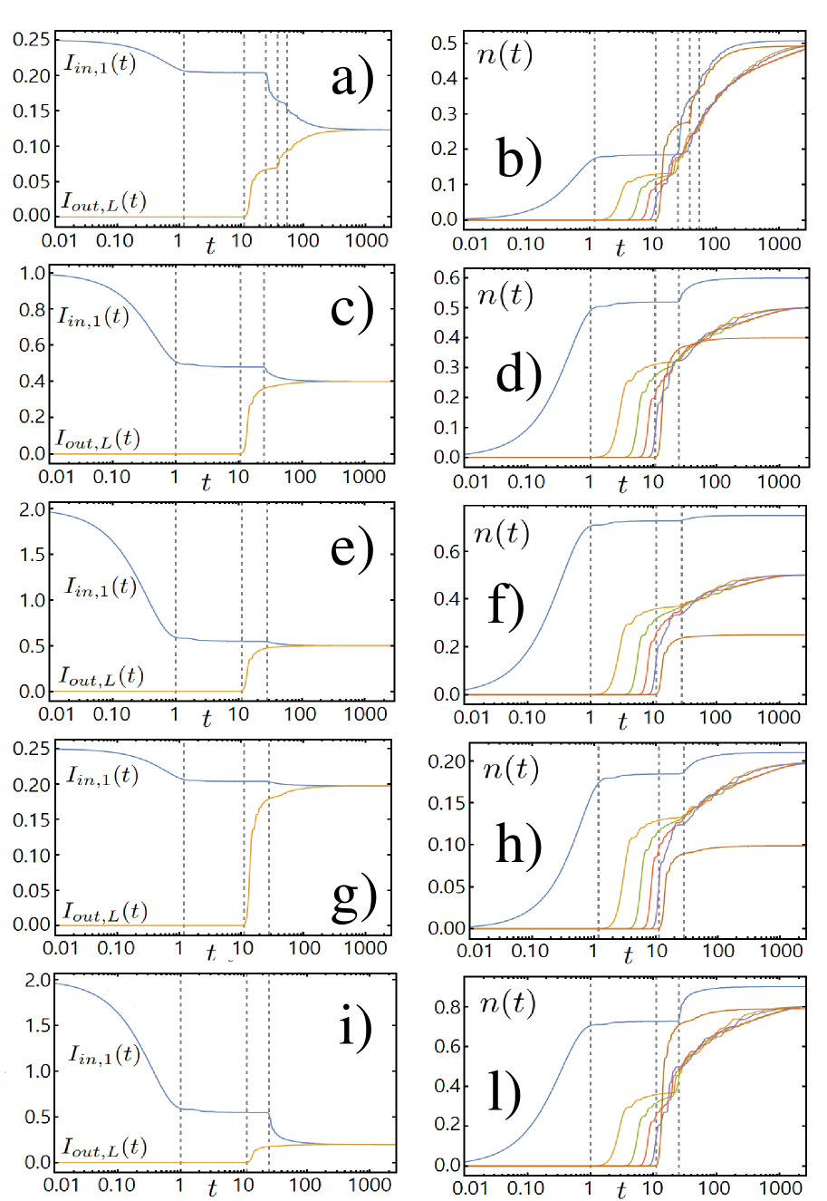
Figure 2:
a): $I_{1,in}(t)$ (blue curve) and $I_{out,L}(t)$ (yellow curve) currents as a function of time $t$ (on a logarithmic scale) measured in units of $J^{-1}$, in an $L=25$ chain with $J=1$ and $\mu=0$, taken to the large bias regime for $(\Gamma_{1}=0.25,\gamma_{L}=0.25)$;
b) $n_{1}(t)$ (blue curve), $n_{5}(t)$ (yellow curve), $n_{10}(t)$ (green curve), $n_{15}(t)$ (red curve), $n_{20}(t)$ (purple curve), and $n_{25}(t)$ (orange curve) computed in the same chain as we used to draw a). The vertical dashed lines mark the boundaries of the plateaus corresponding to quasistationary NESSs (see the main text for the discussion of this point);
c) Same as in a), but with $(\Gamma_{1}=1,\gamma_{L}=1)$;
d) Same as in b), but with $(\Gamma_{1}=1,\gamma_{L}=1)$;
e) Same as in a), but with $(\Gamma_{1}=2,\gamma_{L}=2)$;
f) Same as in b), but with $(\Gamma_{1}=2,\gamma_{L}=2)$;
g) Same as in a), but with $(\Gamma_{1}=0.25,\gamma_{L}=2)$;
h) Same as in b), but with $(\Gamma_{1}=0.25,\gamma_{L}=2)$;
i) Same as in a), but with $(\Gamma_{1}=2,\gamma_{L}=0.25)$;
l) Same as in b), but with $(\Gamma_{1}=2,\gamma_{L}=0.25)$. All the plots are drawn by setting $J=1$ and $\mu=0$.

Due to the asymmetric role played by the couplings between the chain and the reservoirs, we see that, even in the absence of interaction, our system can reach a NESS, provided one waits a long enough time (note that, in the case of symmetric couplings, in order for the system to reach a NESS in a finite time one has to have a nonzero interaction Benenti et al. (2009a)). To evidence this point, in Fig.2 we draw $I_{in,1}(t)$ and $I_{out,L}(t)$, as well as $n_{j}(t)$ at selected lattice sites, in a noninteracting $L=25$ chain with $J=1$ and $\mu=0$ connected to two reservoirs, with the parameters selected as discussed above. In particular, in Fig.2a), c), e), g), i), we draw both $I_{in,1}(t)$ (blue curve) and $I_{out,L}(t)$ (yellow curve) as a function of time (measured in units of $J^{-1}$), by initializing our system at $t=0$ and by assuming that $n_{j}(t=0)=0$ $\forall j$. Moving from plot to plot, we change the couplings to the reservoirs, $\Gamma_{1},\gamma_{L}$, as detailed in the figure caption. By synoptically looking at all the plots, we note the important common feature that, whatever the values of $\Gamma_{1}$ and of $\gamma_{L}$ are, the chain always reaches a NESS at a finite time $t_{\rm NESS}$, corresponding at the point where the blue and the yellow curves merge into each other. In addition to $t_{\rm NESS}$, we also evidence other (preceding) values of $t$ at which the currents reach values that keep stationary for pretty large intervals of time.

To physically interpretate the onset of the plateaus in the current, in Fig.2b), d), f), h), l) we display $n_{j}(t)$ at selected sites of the chain as a function of $t$. In particular, in each plot we show $n_{1}(t)$ (blue curve), $n_{5}(t)$ (yellow curve), $n_{10}(t)$ (green curve), $n_{15}(t)$ (red curve), $n_{20}(t)$ (purple curve), and $n_{25}(t)$ (orange curve). The values of $\Gamma_{1}$, $\gamma_{L}$ are the same as for the corresponding plots at the left-hand side (see figure caption for details). Over all, we observe a similar qualitative behavior for all the plots, with $\Gamma_{1}$ and $\gamma_{L}$ only affecting numerical values of the various quantities. At the start, we see that electrons enter from site $j=1$ and start to fill the chain by propagating to the right. During this “pure filling” phase all the local densities increase in time, in decreasing order, from the one corresponding to the leftmost site ($j=1$). In particular, at about $t=1$ (marked by the leftmost dashed vertical line in the plots), the entering current and density at the boundary site $j=1$ reach “quasistationary” values that keep constant for a large interval of values of $t$ and only depend on $\Gamma_{1}$ (and on $J$, of course). These values correspond to what would be the “true” NESS solution in the thermodynamic limit, $L\rightarrow\infty$. Instead, in our chain the finite size effects determine a breakdown of the NESS above. Indeed, at $t\sim 10$ (second dashed vertical line from the left), electrons have had enough time to reach the endpoint of the chain opposite to the injection point. Accordingly, the density at $j=L$ starts to grow. At the same time, the outgoing current increases with a slope depending on $\gamma_{L}$. However not all the electrons reaching the endpoint of the chain exit to the right-hand reservoir: a finite fraction of them is backscattered toward the left-hand endpoint. This gives rise to a “countercurrent”, flowing from the right to the left, and to a corresponding further increase of the local densities, this time in reverse order ($j=L$ first). The countercurrent and the further increase of the local densities are exactly the features that take the system out of the first putative NESS to a second putative NESS, corresponding to the second shorter plateau in the plots of Fig.2. They are a consequence of having a finite-$L$ chain and, as we argue above, are expected to disappear as $L\to\infty$, where the putative NESS becomes the actual NESS of the system.

Going further ahead in time, at $t\sim 28$ (third dashed vertical line from the left), the countercurrent hits the left-hand endpoint of the chain, with the effect of further increasing $n_{1}(t)$ and of reducing the incoming current. At this point, the second NESS breaks down, as well. Going ahead in time, we see that electrons propagate back and forth inside the chain, with a series of consecutive bounces that manifest themselves in the plots as a series of steps and plateaus, till the system reaches the “true”, asymptotic NESS. The number, the size and the distance of the steps, as well as the details of the asymptotic NESS, depend in a non trivial way on $\Gamma_{1}$ and $\gamma_{L}$.

Looking at the plots in Fig.2 we readily note that the NESS is characterized by the convergence (in time) of $I_{in,1}(t)$ and of $I_{out,L}(t)$ towards a single, time independent, value of the current, $I_{\rm st}$, that is a typical feature of the stationary state. Moreover, we also see that $n_{j}(t)$ at any site $j\neq 1,L$ flows toward a unique value $n_{\rm st}$, thus yielding a profile of the real space electron density in the NESS, $n_{{\rm st},j}$, constant everywhere but at the endpoints of the chain. Whether the system is interacting, or not, throughout all the paper we characterize the NESS in terms of $I_{\rm st}$ and of $n_{{\rm st},j}$, in particular referring to $n_{\rm st}$ in the flat part of the density profile. In the noninteracting case, both $I_{\rm st}$ and $n_{\rm st}$ can be analytically determined. Specifically, using Eq.(14), we obtain

$$I_{\rm st} = \lim_{t\rightarrow\infty}\{\Gamma_{1}(1-n_{1}(t))-\gamma_{1}n_{1}(t)\}$$

$$= \lim_{t\rightarrow\infty}\{-\Gamma_{L}(1-n_{L}(t))+\gamma_{L}n_{L}(t)\}$$

$$= \frac{4J^{2}(\Gamma_{1}\gamma_{L}-\gamma_{1}\Gamma_{L})}{(\Gamma_{1}+\gamma_{1}+\Gamma_{L}+\gamma_{L})[4J^{2}+(\Gamma_{1}+\gamma_{1})(\Gamma_{L}+\gamma_{L})]}\>\>\>\>.$$

From Eq.(III), we see that, as it must be, $I_{\rm st}$ is independent of $L$: the length of the chain only affects the time windows corresponding to each putative NESS. Similarly, defining $n_{\rm st}$ as

$$n_{\rm st}=\lim_{t\rightarrow\infty}\frac{1}{L-2}\sum_{i=2}^{L-1}\>n_{i}(t)\>\>\>\>,$$ (18)

we obtain

$$n_{\rm st}=$$ (19)

$$\frac{4J^{2}(\Gamma_{1}+\Gamma_{L})+\gamma_{1}^{2}\Gamma_{L}+\Gamma_{1}[(2\gamma_{1}+\Gamma_{1})\Gamma_{L}+(\gamma_{L}+\Gamma_{L})^{2}]}{(\Gamma_{1}+\gamma_{1}+\Gamma_{L}+\gamma_{L})[4J^{2}+(\Gamma_{1}+\gamma_{1})(\Gamma_{L}+\gamma_{L})]}\>\>\>\>,$$

which, as expected, is independent of $L$, as well.

From Eq.(19) we see that $n_{\rm st}=1/2$ for any values of $f$ and $g$ in the symmetric regime and for $\Gamma_{1}=\gamma_{L}$ in the large bias regime. At variance, at generic values of $\Gamma_{1}$ and $\gamma_{L}$ and in the large bias regime, we find

$$n_{\rm st}=\frac{\Gamma_{1}(4J^{2}+\gamma_{L}^{2})}{(\Gamma_{1}+\gamma_{L})(4J^{2}+\Gamma_{1}\gamma_{L})}\>\>\>\>.$$ (20)

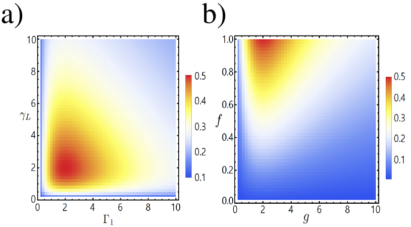
Figure 3:
a): $I_{\rm st}$ computed in the $L=25$ chain for $J=1$ and $\mu=0$ both as a function of $\Gamma_{1}$ and $\gamma_{L}$ in the large bias limit;
b): $I_{\rm st}$ as a function of $f$ and $g$ in the symmetric regime $\Gamma_{1}=\gamma_{L}$. Red areas correspond to high values of $I_{\rm st}$, blue areas to low values (see the color code for details).

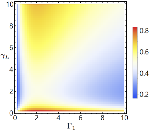
Figure 4: $n_{\rm st}$ computed in the $L=25$ chain for $J=1$ and $\mu=0$ as a function of $\Gamma_{1}$ and $\gamma_{L}$ in the large bias limit. Red areas correspond to high values of $n_{\rm st}$, blue areas to low values (see the color code for details).

To highlight the main features of our chain in the absence of interaction, in Fig.3 we plot $I_{\rm st}$ both as a function of $\Gamma_{1}$ and $\gamma_{L}$ in the large bias limit (Fig.3a)) , and as a function of $f$ and $g$ in the symmetric regime $\Gamma_{1}=\gamma_{L}$ (Fig.3b)) , while in Fig.4 we plot $n_{\rm st}$ in the large bias regime. Two interesting features emerge. First, we observe the emergence of an OWP in the $\Gamma_{1}-\gamma_{L}$ parameter space at which $I_{\rm st}$ is maximum. Specifically, from Fig.3 we see that the OWP corresponds to $f=1$ (largest possible bias), and to symmetric couplings, $\Gamma_{1,max}=\gamma_{L,max}=g_{max}=2$. Second, synoptically considering $I_{\rm st}$ in Fig.3 and $n_{\rm st}$ in Fig.4, we note that the former is, in general, a non-monotonic function of the latter. In particular, we see that for both high- and low-values of $n_{\rm st}$, $I_{\rm st}$ is lower than its maximum value $1/2$. This is a typical behavior found in fundamental traffic flow diagrams Nagatani (2002, 1998), where the free flow phase and the congested phases are separated by an optimal value of the density, at which the traffic flow (the “current”) is maximum. So, from Figs.3 and 4 we see that our system might potentially work as a “quantum simulator” of the fundamental traffic flow diagram. Aside the fascinating correspondence with traffic flow phase diagram, we definitely evidence how pertinently managing for the couplings between the chain and the reservoirs may affect in a nontrivial way the current propagation into the system.

In order to compare the LE formalism with alternative approaches to nonequilibrium transport problems, such as the non-equilibrium Green function, or the Landauer-Büttiker method, we refer to the detailed analysis of Ref.[Guimarães et al., 2016]. In particular, we note that, while we do not expect any substantial qualitative difference between the results obtained within those two methods and ours, in order to exactly reproduce the results using the LE method for $U=0$ one should generalize the LE to the case of multisite reservoirs, as extensively discussed, and rigorously proven, in Ref.[Guimarães et al., 2016] , where it is shown how the expression for the nonequilibrium steady-state current of a quantum chain coupled to two multisite reservoirs at both boundaries, each one consisting of $L_{Res}$ sites, reduces back to the Landauer-Büttiker formula for the electronic current through a tunneling junction, in the limit $L_{Res}\to\infty$ and for a small voltage bias between the two reservoirs.

We now generalize our discussion to the case in which a nonzero electron interaction turns on in the chain.

IV One-dimensional spinless Hubbard chain

Turning on a finite on-site interaction strength $U$ in the chain described by $H_{c}$ in Eq.(15), we get the Hamiltonian $H_{i}$ given by

$$H_{i}=-J\sum_{j=1}^{L-1}\{c_{j}^{\dagger}c_{j+1}+c_{j+1}^{\dagger}c_{j}\}-\mu\sum_{j=1}^{L}c_{j}^{\dagger}c_{j}+U\sum_{j=1}^{L-1}n_{j}n_{j+1}\>\>\>\>.$$ (21)

$H_{i}$ in Eq.(21) is 1HM Hamiltonian over an $L$-site chain Essler et al. (2005). To recover it from the generic $H$ in Eq.(1), we simply set $N=L$, $[{\cal H}_{0}]_{j,k}=-J\{\delta_{j,k+1}(1-\delta_{k,L})+\delta_{j,k-1}(1-\delta_{k,1})\}-\mu\delta_{j,k}$, and $[{\cal H}_{U}]_{j,k}=U\{\delta_{j,k+1}(1-\delta_{k,L})+\delta_{j,k-1}(1-\delta_{k,1})\}$.

Beside being a paradigmatic model for one-dimensional correlated electronic systems, the 1HM also provides an equivalent description of an $XXZ$ spin-1/2 quantum spin chain, which is mapped onto it via the Jordan-Wigner transformation Jordan and Wigner (1928). Therefore, by the same token, when connecting the external reservoirs to the 1HM described by $H_{i}$ in Eq.(21), we also recover a mean to study the spin current across a quantum spin chain connected to external reservoirs Benenti et al. (2009b, a); Langer et al. (2009); Xianlong et al. (2008). Moreover, the 1HM has also been shown to effectively describe a one-dimensional lattice model of interacting bosons in the limit of strong on-site repulsion between bosons, once the chemical potential is tuned so to make the states at each site populated with $n$ and $n+1$ bosons to be degenerate with each other Giuliano et al. (2013). Therefore, we expect our analysis of the interacting fermionic chain to be of relevance for all the different physical systems effectively described by the 1HM.

$H_{i}$ in Eq.(21) is a simple, prototypical example of a strongly correlated fermionic model. While the LE approach can be implemented in order to study the equilibrium properties of a quantum system, we do not expect that the mean field approximation works in the equilibrium case for one-dimensional electronic chains. Instead, in this regime different methods, such as the functional renormalization group Markhof et al. (2018) or the Thermodynamic Bethe Ansatz Takahashi and Shiroishi (2002), can be used to study the phase diagram of the system. Both methods can be successfully extended to nonequilbrium systems: the Thermodynamic Bethe Ansatz can be implemented successfully to analyze nonequilibrium homogeneous quantum chains Castro-Alvaredo et al. (2014), or quantum impurity models Mehta and Andrei (2006); nonequilibrium extensions of the functional renormalization group approach have been proposed to study the non equilibrium properties of a quantum wire coupled to two reservoirs Jakobs et al. (2007); Berges and Mesterházy (2012).

In one spatial dimension, it is well known that, to analytically describe equilibrium physics of the 1HM, one has to resort to sophisticated mathematical techniques, such as the bosonic Luttinger liquid (LL) approach (see, for instance, Ref.[Giamarchi, 2003] for a comprehensive review on the subject). As LL is basically a low-energy, long-wavelength effective theory for the correlated fermionic system, its applications to strongly out-of-equilibrium states, such as the ones we discuss here, are not straightforward, not even after resorting to clever out-of-equilibrium implementation of the method, such as the one based on the nonequilibrium functional renormalization group approach Jakobs et al. (2007). As it is out forward in detail in Refs.[Benenti et al., 2009a; Brenes et al., 2018] and as we discuss in detail in the following, the NESS that sets in in the nonequilibrium chain corresponds to a (combination of) highly-excited states of $H_{i}$ in Eq.(21), which are expected to be out-of-reach of the standard LL approach. Moreover, while nonequilibrium renormalization group approach might in principle be employed to recover the NESS in the nonequilibrium 1HM, the unavoidable technical difficulty of extending the approach beyond the regime of weak coupling between the reservoirs and the system makes it pretty challenging to recover the density profile and the current pattern characterizing the NESS. At variance, as we highlight below, our MF approximation provide a simple analytical mean to access features of the NESS that are in a good agreement with results recovered within alternative numerical methods Benenti et al. (2009a, b); Brenes et al. (2018).

In general, $U$ can either be positive, or negative. In the following we restrict ourselves to the $U\geq 0$ case only. The negative-$U$ 1HM can nevertheless be straightforwardly analyzed by methods analogous to the ones we employ here. Also, in all our calculations, we set $\mu$ according to the condition that, at equilibrium, the chain is half-filled. This implies choosing $\mu$ so to cancel the chemical potential renormalization due to a finite $U$. A simple calculation provides the condition $\mu_{\rm eff}=0$, with $\mu_{\rm eff}=\mu+\frac{U}{2}$. In the following, we assume that this condition is already satisfied, unless explicitly stated otherwise. To analyze the 1HM connected to the external reservoirs, we systematically implement the MF decoupling of Eq.(9). In fact, at the price of using an effective, time-dependent Hamiltonian in the LE, the MF massively eases the numerical solution of the LE, compared to fully numerical approaches Benenti et al. (2009b, a); Langer et al. (2009); Xianlong et al. (2008); Mühlbacher and Rabani (2008), thus allowing for exploring pretty large windows of variations of the system parameters.

Applying Eq.(9) to the interaction $Un_{j}n_{j+1}$, we obtain the corresponding MF decoupling

$$Un_{j}n_{j+1} \to U\{n_{j}(t)n_{j+1}+n_{j}n_{j+1}(t)$$ (22)

$$- {\cal I}_{j+1,j}(t)c_{j}^{\dagger}c_{j+1}-{\cal I}_{j,j+1}(t)c_{j+1}^{\dagger}c_{j}\}\;\;\;\;,$$

with the explicit dependence on $t$ of the average values being a direct consequence of the nonequilibrium due to the coupling to the reservoirs. In principle, to determine the time evolution of the system within MF approximation, we have to solve Eq.(2) for $\rho(t)$ using the Lindblad operators in Eqs.(3) and the time-dependent Hamiltonian $\tilde{H}_{i}(t)$, given by

$$\tilde{H}_{i}(t)=$$ (23)

$$-\sum_{j=1}^{L-1}\{[J+U{\cal I}_{j+1,j}(t)]c_{j}^{\dagger}c_{j+1}+[J+U{\cal I}_{j,j+1}(t)]c_{j+1}^{\dagger}c_{j}\}$$

$$-\sum_{j=1}^{L}[\mu+Un_{j-1}(t)(1-\delta_{j,1})+Un_{j+1}(t)(1-\delta_{j,L})]n_{j}\;\>\>\>.$$

Nevertheless, $\tilde{H}_{i}(t)$ contains time-dependent averages of operators, which require the explicit knowledge of the density matrix at time $t$, in order to be computed. For this reason, we numerically solve the nonlinear ME equations (Eq.(II)), directly written for the time-dependent averages $n_{j}(t)$ and ${\cal I}_{j,j\pm 1}(t)$. Numerically integrating the nonlinear equations and taking the large-time limit of the final result, we eventually extend to the interacting case the characterization of the NESS in terms of $I_{\rm st}$ and of $n_{{\rm st},j}$.

In Fig.5 we plot $I_{in,1}(t)$ (blue curve) and $I_{out,L}(t)$ (yellow curve) as a function of $t$ (on a logarithmic scale) measured in units of $J^{-1}$, in an $L=20$ chain with $J=1$ and $\mu_{\rm eff}=0$, in the large-bias regime, with $\Gamma_{1}=\gamma_{L}=g=1$, for $U=1$ (Fig.5a)), and for $U=0$ (Fig.5b)). In both cases we set the initial state of the chain with $n_{j}(t=0)=0$ $\forall j$. While, from the qualitative point of view, we see no relevant differences between the two plots, quantitatively we note a remarkable reduction in $I_{\rm st}$ for $U=1$. Such a behavior is known from numerical simulations to emerge in the out-of-equilibrium chain, due to the peculiar nonequilibrium charge density distribution (spin magnetization distribution in the corresponing $XXZ$ spin chain) that sets in the system at the NESS Benenti et al. (2009a); Brenes et al. (2018). While we extensively discuss about this point in the following of this Section, we now consider Fig.6, where we plot the average particle densities at various sites, computed for the same values of the system parameters we used to draw Fig.5, for $U=1$ (left-hand plot) and for $U=0$ (right-hand plot). Specifically, in both plots we draw $n_{1}(t)$ (blue curve), $n_{5}(t)$ (yellow curve), $n_{10}(t)$ (brown curve), $n_{15}(t)$ (orange curve), and $n_{20}(t)$ (purple curve). Apparently, the interacting case is qualitatively similar to the noninteracting one, except that it takes a longer time for the sites distant from the current injection point to be filled with particles, due to the repulsive interaction between electrons.

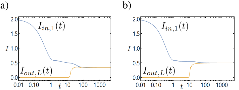
Figure 5:
a): $I_{in,1}(t)$ (blue curve) and $I_{out,L}(t)$ (yellow curve) currents as a function of time $t$ (on a logarithmic scale) measured in units of $J^{-1}$, in an $L=20$ interacting chain with $U=1$, taken to the large bias regime for $\Gamma_{1}=\gamma_{L}=g=1$, $J=1$, and $\mu_{\rm eff}=0$.
b): Same as in a), but with $U=0$.

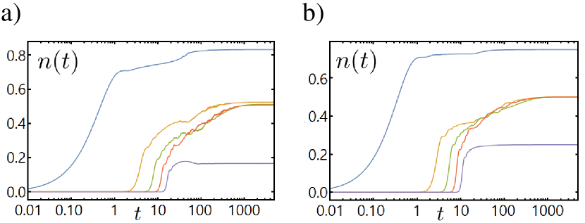
Figure 6:
a): $n_{1}(t)$ (blue curve), $n_{5}(t)$ (yellow curve), $n_{10}(t)$ (brown curve), $n_{15}(t)$ (orange curve), and $n_{20}(t)$ (purple curve) as a function of time $t$ (on a logarithmic scale) measured in units of $J^{-1}$, in an $L=20$ interacting chain with $U=1$, taken to the large bias regime for $\Gamma_{1}=\gamma_{L}=g=1$, $J=1$, and $\mu_{\rm eff}=0$;
b): Same as in a), but with $U=0$.

To characterize the NESS, we look at the dependence of $I_{\rm st}$ and of $n_{{\rm st},j}$ on the system parameters, starting from the interaction strength $U$. In Fig.7, we plot $I_{\rm st}$ as a function of $U$ for specific values of the interaction, ranging from $U=0$ to $U=2$. $I_{\rm st}$ is finite, though decreasing with $U$, as long as $\frac{U}{J}\leq 2$. At $\frac{U}{J}=2$, $I_{\rm st}$ becomes zero and keeps zero at any $U>2J$. Apparently, this is a conductor-to-insulator transition that, once one goes through the appropriate Jordan-Wigner transformation, is the analog of the behavior of the spin current across an $XXZ$ chain connected to two reservoirs kept at large bias, when the Ising anisotropy $\Delta>1$ (which corresponds to $\frac{U}{J}>2$ in our units) Benenti et al. (2009b).

About the onset of the insulating phase, it is worth pointing out, here, that it is different from the Mott transition toward the insulating charge density wave (CDW) phase that takes place at large enough $U$ in the 1HM close to half-filling Giamarchi (2003). Indeed, the CDW sets in as an ordered, staggered pattern in the spatial charge distribution in the equilibrium state of the chain. Instead, in the nonequilibrium 1HM we recover a fully different NESS, as we discuss in detail next.

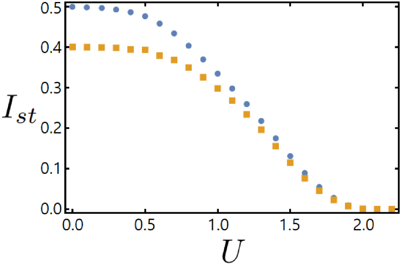
Figure 7: $I_{\rm st}$ as a function of $U$ in an $L=20$ chain with $J=1,\mu_{\rm eff}=0$, computed in the large bias limit, with $\Gamma_{1}=\gamma_{L}=g=1$ (orange squares) and with $\Gamma_{1}=\gamma_{L}=g=2$ (blue circles). There is an apparent conductor to insulator transition at $U=2$ in both cases.

To discuss the nonequilibrium NESS in the interacting model, we refer to Ref.[Benenti et al., 2009b], where it is noted how, when connecting a spin-1/2 $XXZ$ spin chain with $\Delta>1$ to two fully polarized spin reservoirs with opposite spin polarizations (which corresponds to our large bias limit), the reservoirs induce a net magnetization within the chain along the same direction of their spin polarization. Being the reservoirs oppositely polarized, at strong enough interaction, a domain wall arises at the center of the chain, where smoothly, though rapidly (in real space) the magnetization profile matches the opposite, “asymptotic” values (see Fig.3 of Ref.[Benenti et al., 2009b] for details). The formation of the domain wall strongly suppresses the spin current across the chain, thus effectively inducing a transition between a “spin conducting” and a “spin insulating” phase. By analogy, in our case we expect a charge domain wall to emerge in the real space profile of $n_{{\rm st},j}$ at $\frac{U}{J}=2$. To check this point, in Fig.8 we plot $n_{{\rm st},j}$, at each site of an $L=20$ chain with $J=1,\mu_{\rm eff}=0$, taken to the large bias limit, with $\Gamma_{1}=\gamma_{L}=g=2$, and with $U=0$ (blue circles - blue interpolating curve), $U=0.5$ (orange squares - orange interpolating curve), $U=1$ (green rhombi - green interpolating curve), $U=1.5$ (red triangles - red interpolating curve), and $U=2$ (purple rotated triangles - purple interpolating curve). While the plot at $U=2$ apparently matches the corresponding one, drawn at $\Delta=1$, in Fig.3 of Ref.[Benenti et al., 2009b], for $\frac{U}{J}<2$, we see extended flat regions in the profile of $n_{{\rm st},j}$, eventually bending upward or downward close to the endpoints of the chain.

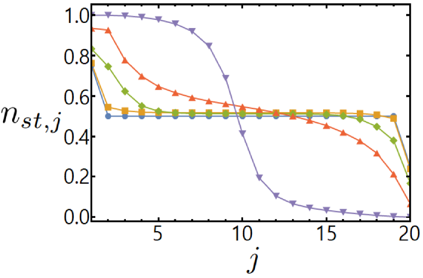
Figure 8: $n_{{\rm st},j}$ at each site $j$ of an $L=20$ chain with $J=1,\mu_{\rm eff}=0$, computed in the large bias limit, with $\Gamma_{1}=\gamma_{L}=g=2$, and with $U=0$ (blue circles - blue interpolating curve), $U=0.5$ (orange squares - orange interpolating curve), $U=1$ (green rhombi - green interpolating curve), $U=1.5$ (red triangles - red interpolating curve), and $U=2$ (purple rotated triangles - purple interpolating curve)

In Appendix A, we provide a physical interpretation of the behavior of $I_{\rm st}$ and of $n_{{\rm st},j}$. In particular, resorting to a simple, though qualitatively effective, variational method combined a pertinent MF approach to the 1HM Misguich et al. (2019), we argue how, in order for our system to support a finite $I_{\rm st}$ for $\frac{U}{J}\leq 2$, there has to be a flat region of values in $n_{{\rm st},j}$ throughout the middle part of the chain, with a respectively upward and a downward turn close to the endpoints of the chain, that are required to match $n_{{\rm st},1}$ and $n_{{\rm st},L}$ as determined by the constancy of $I_{\rm st}$. On increasing $U$, the flat region shortens, till it shrinks at $U=2$, by taking a “kink-like” profile, with a corresponding blocking of the current transport ($I_{\rm st}=0$), for $U\geq 2$ Benenti et al. (2009a, b). Therefore, when characterizing the NESS by looking at $I_{\rm st}$ and of $n_{{\rm st},j}$, we are apparently led to associate the emergence of a flat density region in the middle of the chain with a finite value of the stationary state current and, at variance, a kink-like profile in the density plot with a blocking of the charge flow, that is, with $I_{\rm st}=0$. The bending of the flat density profile as $\frac{U}{J}$ increases corresponds to the reduction of $I_{\rm st}$ at increasing $U$, which we display in Fig.5.

To discuss the emergence of the OWP in the extended parameter space including $U$ and the coupling strengths, we first, following Ref.[Benenti et al., 2009a], look at the maximum value of $I_{\rm st}$ as a function of $f$ in an $L=20$ chain with $J=1,\mu_{\rm eff}=0$, in the symmetric case and for various values of $U$ (Fig.9a)). Then, we extend the parameter space by considering $I_{\rm st}$ as a function of $g$ in the same chain, in the large-bias limit, for $\Gamma_{1}=\gamma_{L}=g$ (Fig.9b)), at increasing values of $U$. As in Ref.[Benenti et al., 2009a], we find that, at finite $U>0$, an OWP emerges, at a value of $f_{\rm OWP}$ at which $I_{\rm st}$ reaches its maximum value. Moreover, the larger is $U$, the more $f_{\rm OWP}$ is pushed towards lower values of $f$. In addition, from Fig.9b), we also recover one the most important original results of our work, that is, that turning on $U$ is not a necessary condition to get the OWP (see also Appendix A for a separate discussion of this point). Indeed, we see a maximum in the plots of $I_{\rm st}$ as a function of $g$ even when $U=0$, provided we tune the system at the large-bias limit. So, we directly prove that, increasing the number of tuning parameters, we may recover the OWP even in regions in parameter space where it does not emerge if the system is close to the equilibrium. More specifically, to make a quantitative comparison with the results of Refs.[Benenti et al., 2009a, b], we focus onto the purple curve of Fig.9a). Apparently, this exhibits a reasonable qualitative agreement with the purple (bottom) curve of Fig.11 of Ref.[Benenti et al., 2009a], though with a stronger bending toward the zero-current axis as $L\to 20$, which is motivated by the slightly larger total number of sites (20 rather than 16) and by the observation that the system should be insulating in the thermodynamic limit at $\frac{U}{J}=2$. More generally, the MF approach is expected to underestimate fluctuations in short chains and, therefore, to work fine for long enough chains. To check this point, in Fig.9c) we plot $I_{\rm st}$ as a function of $f$ with the same system parameters used to draw Fig.9a), for $L=4$ (blue dots, blue interpolating curve) and for $L=16$ (yellow squares, yellow interpolating curve). We note a better agreement between the corresponding plots of Fig.11 of Ref.[Benenti et al., 2009a] relative to the longer chain ($L=16$), rather than the shorter one ($L=4$).

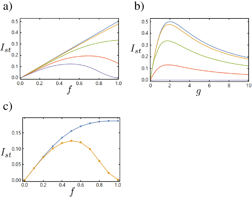
Figure 9:
a): $I_{\rm st}$ as a function of $f$, with $g$ set so that $I_{\rm st}$ is maximum, computed in an $L=20$ chain with $J=1$, $\mu_{\rm eff}=0$, and $U=0$ (blue curve), $U=0.5$ (yellow curve), $U=1$ (green curve), $U=1.5$ (red curve) and $U=2$ (purple curve);
b): Maximum value of $I_{\rm st}$ as a function of $g$ in the large bias regime for $g=\Gamma_{1}=\gamma_{L}$. The system parameters and the color code for the curves drawn at different values of $U$ are the same as in the left-hand plot;
c): $I_{\rm st}$ as a function of $f$, with $g$ set so that $I_{\rm st}$ is maximum, computed in a chain with $J=1$, $\mu_{\rm eff}=0$, $U=2$, with $L=4$(blue dots, blue interpolating curve) and with $L=16$ (yellow squares, yellow interpolating curve).

To conclude this Section, we briefly discuss the dependence of the NESS on the initial state of the system. This is an important point to verify, so to make sure that the NESS is unique and there are no “bifurcations” in the time evolution described by Lindblad equations, which in some cases may affect the time evolution of the system toward the NESS Nava and Fabrizio (2019). In particular, in Fig.10a) we show $I_{in,1}(t)$ (blue curve) and $I_{out,L}(t)$ (yellow curve) as a function of time $t$ in the same system as the ones we have used to derive Figs.5,6, but with the initial state characterized by $n_{j}(t=0)=1$ $\forall j$. While the evolution in time of the two currents is completely different from the one that we report in Fig.5a), we see that, as $t\to\infty$, they converge to the same $I_{\rm st}$ as in the case in which one has $n_{j}(t=0)=0$ $\forall j$. For comparison, in Fig.10b), we draw $n_{1}(t)$ (blue curve), $n_{5}(t)$ (yellow curve), $n_{10}(t)$ (green curve), $n_{15}(t)$ (orange curve), and $n_{20}(t)$ (purple curve) as a function of time $t$. Except for the green curve, we find an acceptable consistency with the values of $n_{{\rm st},j}$ extrapolated from Fig.6a). Being the density a local operator, it is strongly affected by the finite size of the chain, by the distance from the reservoirs, et cetera. Likely, working with longer chains and extrapolating the results over longer time would wash out this discrepancy, as well. So, we may readily infer that, though the initial states in the two cases are completely different, the NESS in the two systems is the same, independently of the initial state.

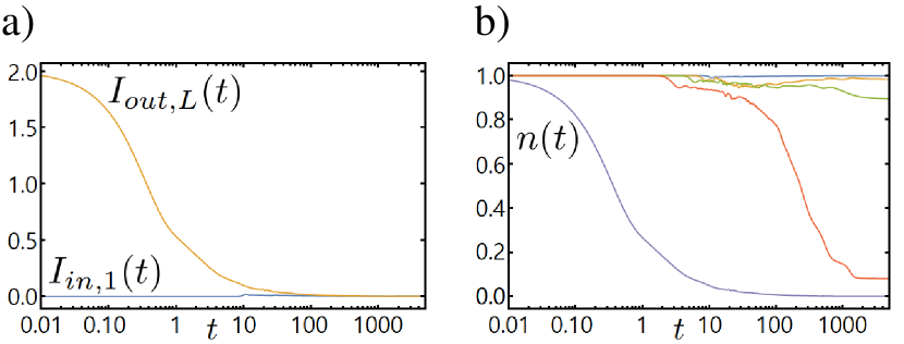
Figure 10:
a): $I_{in,1}(t)$ (blue curve) and $I_{out,L}(t)$ (yellow curve) currents as a function of time $t$ (on a logarithmic scale) measured in units of $J^{-1}$, in an $L=20$ interacting chain with $J=1$, $\mu_{\rm eff}=0$, and $U=2$, taken to the large bias regime for $\Gamma_{1}=1,\gamma_{L}=g=1$, $J=1$, with the system prepared, at $t=0$ in the state with $n_{j}(t=0)=1$ $\forall j$;
b): $n_{1}(t)$ (blue curve), $n_{5}(t)$ (yellow curve), $n_{10}(t)$ (green curve), $n_{15}(t)$ (orange curve), and $n_{20}(t)$ (purple curve) as a function of time $t$ (on a logarithmic scale) measured in units of $J^{-1}$, in an $L=20$ interacting chain with $J=1$, $\mu_{\rm eff}=0$, and $U=2$, taken to the large bias regime for $\Gamma_{1}=1,\gamma_{L}=g=1$, $J=1$, with the system prepared, at $t=0$ in the state with $n_{j}(t=0)=1$ $\forall j$.

We now discuss the effects of nonzero disorder on the time evolution of our system and on the formation of the corresponding NESS. To do so, we first discuss the case of a single, isolated defect in the chain (an “impurity”). Therefore, we consider a finite density of random impurities in the chain (“quenched disorder”).

V A single impurity in the chain at large bias

Impurities in a quantum chain can be either realized by tuning $\mu_{\rm eff}$ at a site $\bar{j}$ to a value $\mu_{d}$ different from all the other sites (“site impurity”), or by changing the electronic hopping strength of a single bond of the chain (“bond impurity”). While the equilibrium physics of impurities in the 1HM (or in the $XXZ$ spin-1/2 quantum spin chain) can be analytically addressed within a number of effective methods, such as LL approach, Eggert and Affleck (1992); Sorensen et al. (1993); Kane and Fisher (1992a, b); Giuliano and Sodano (2005); Giuliano et al. (2017, 2018), it is definitely challenging to analytically deal with transport across impurities in the 1HM connected to reservoirs in the large bias limit, even after resorting to powerful analytical methods, such as the functional renormalization group approach developed in Ref.[Jakobs et al., 2007]. Nevertheless, as we discuss in this Section, despite its simplicity, our MF approach is able to catch the relevant physics of the NESS state in the out-of-equilibrium 1HM.

First of all, we recall that both the 1HM and $XXZ$ spin chain are integrable models. In general, the conservation laws associated to integrability are known to prevent the system from thermalizing toward a state characterized by a macroscopic hydrodynamical behavior in its transport properties Zotos et al. (1997); Benenti et al. (2013). On this respect, a crucial problem is analyzing how a perturbation breaking the integrability of the system (even locally) affects the evolution toward the NESS in the large bias limit Rigol (2009). In this direction, the simplest possible way of breaking integrability is by just making the system inhomogeneous by adding a local impurity term to the otherwise integrable Hamiltonian.

Following the approach of Ref.[Brenes et al., 2018], in this Section we analyze how adding an impurity term to the Hamiltonian in Eq.(21) affects the evolution of the system toward the NESS, and the structure of the NESS itself, once the chain is connected to the reservoirs out of equilibrium. For the sake of simplicity in both cases, with no loss of generality, we symmetrically realize the impurity at the center of the chain, which requires $L$ to be odd for the site impurity and even for the bond impurity.

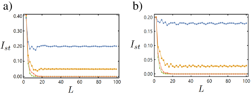
Figure 11:
a): $I_{\rm st}$ as a function of $L$ computed in the 1HM with a site impurity of strength $\mu_{d}=1.5$, with $J=1$ and $U=1.0$ (blue circles, blue interpolating curve), $U=1.7$ (yellow squares, yellow interpolating curve), $U=2.0$ (orange triangles, orange interpolating curve), $U=3.0$ (green rhombi, green interpolating curve);
b): $I_{\rm st}$ as a function of $L$ computed in the 1HM with a bond impurity of strength $J_{d}=0.5$, with $J=1$ and $U=1.0$ (blue circles, blue interpolating curve), $U=1.7$ (yellow squares, yellow interpolating curve), $U=2.0$ (orange triangles, orange interpolating curve), $U=3.0$ (green rhombi, green interpolating curve)

To check the reliability of our method, in the case of the site impurity we compare our results with the analogous ones of Ref.[Brenes et al., 2018] obtained within $t$-DMRG approach. Taking $L$ odd, we realize the site impurity by adding to $H_{i}$ in Eq.(21) the impurity Hamiltonian $H_{\rm site}$ given by

$$H_{\rm site}=-\mu_{d}n_{\frac{L+1}{2}}=-\mu_{d}c^{\dagger}_{\frac{L+1}{2}}c_{\frac{L+1}{2}}\>\>\>\>.$$ (24)

As we have done in the homogeneous case, we characterize the NESS by looking at $I_{\rm st}$ and at $n_{{\rm st},j}$. To highlight the effects of increasing the impurity interaction strength, in Fig.12a) we show $n_{{\rm st},j}$, computed in an 1HM with $L=19$, $J=1$, $\mu_{\rm eff}=0$, and $U=0$, in the large bias limit with $\Gamma_{1}=\gamma_{L}=g=2$, with the impurity symmetrically located at site $\bar{j}=10$, at various values of the on-site chemical potential $\mu_{d}$ (see figure caption for details). At variance, to evidence the effects of the bulk interaction, in Fig.12b) we again show $n_{{\rm st},j}$, computed for the same parameters as in the left-hand plot, except that now we fix $\mu_{d}=1.5$ and vary $U$ from plot to plot (see figure caption for details). Finally, to make sure that there are no finite-size effects spoiling our results, we compute $I_{\rm st}$ as a function of $L$ for both the site impurity and the bond impurity for selected values of $U$ up to $L\sim 100$, where, as we show in Fig.11a) for the site impurity and in Fig.11b) for the bond impurity, apparently $I_{\rm st}$ has reached its asymptotic value in the thermodynamic limit.

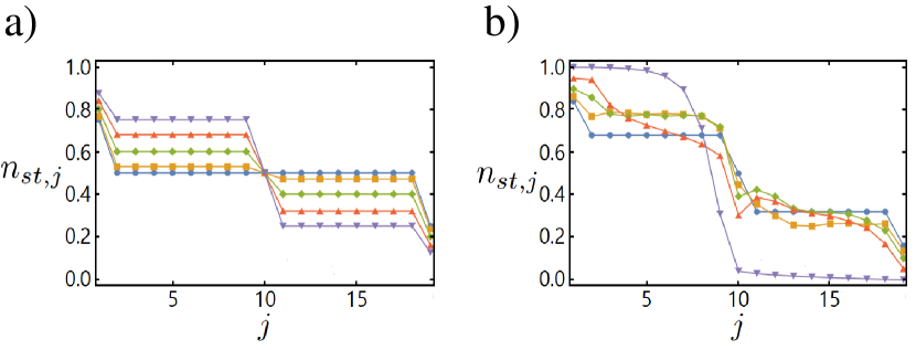
Figure 12:
a): $n_{{\rm st},j}$, computed in an HM with $L=19$, $J=1$, $\mu_{\rm eff}=0$, and $U=0$, in the large bias limit with $\Gamma_{1}=\gamma_{L}=g=2$, with a site corresponding to the Hamiltonian in Eq.(24) with $\mu_{d}=0.0$ (blue dots, blue interpolating curve), $\mu_{d}=0.5$ (orange squares, orange interpolating curve), $\mu_{d}=1.0$ (green rhombi, green interpolating curve), $\mu_{d}=1.5$ (red upward pointing triangles, red interpolating curve), and $\mu_{d}=2.0$ (purple downward pointing triangles, purple interpolating curve);
b): $n_{{\rm st},j}$, computed in an HM with $L=19$, $J=1$, $\mu_{\rm eff}=0$, in the large bias limit with $\Gamma_{1}=\gamma_{L}=g=2$, with a site corresponding to the Hamiltonian in Eq.(24) with $\mu_{d}=1.5$, computed for $U=0.0$ (blue dots, blue interpolating curve), $U=0.5$ (orange squares, orange interpolating curve), $U=1.0$ (green rhombi, green interpolating curve), $U=1.5$ (red upward pointing triangles, red interpolating curve), and $U=2.0$ (purple downward pointing triangles, purple interpolating curve).

By synoptically looking at the plots in Fig.12, we readily note that a nonzero $\mu_{d}$ triggers the emergence of a kink in the middle of the chain, even for $\frac{U}{J}\leq 2$. This feature appears similar to the formation of the kink in the middle of the chain that marks the transition from the conducting to the insulating phase of the nonequilibrium 1HM (see Ref.[Benenti et al., 2009b] as well as our Appendix A for a detailed discussion of this point). However, the persistence of finite regions in real space where the density keeps flat, a feature that is associated to the conducting phase of the 1HM Brenes et al. (2018), is already a clue that the NESS in the presence of a site impurity is only quantitatively, not qualitatively, different from the NESS that sets in the homogenous chain for $\frac{U}{J}\leq 2$. To double check this conclusion, in Fig.13 we plot $I_{\rm st}$ as a function of $\mu_{d}$ computed in the same $L=19$ chain we used to derive the plots of Fig.12, with $J=1$, $\mu_{\rm eff}=0$, and $U=0$ (Fig.12a)), and $U=1.5$ (Fig.12b)), in the large bias limit with $\Gamma_{1}=\gamma_{L}=g=2$. Whether $U=0$ or $U$ takes a finite value, we see that while, turning on $\mu_{d}$ slightly reduces $I_{\rm st}$, at the same time the current keeps finite within the NESS. This enforces the conclusion that turning on a site impurity in the chain does not qualitatively affect the NESS. Therefore, we conclude that both in the case of a homogeneous 1HM, as well as in the presence of a site impurity, our system flows toward a conducting NESS, with an extended, flat regions in the profile of $n_{{\rm st},j}$ in the middle of the chain, and with a finite value of $I_{\rm st}$. In fact, as discussed in detail in Ref.[Brenes et al., 2018], for this range of values of $\frac{U}{J}$ $I_{\rm st}$ is expected to scale with $L$ as $L^{-\nu}$, with $\nu=0$, that is, what is expected for a ballistic conducting channel. Indeed, as we show in Fig.11a), that is what we find within our MF approach, with also a reduction in the (uniform) value of $I_{\rm st}$ as $\frac{U}{J}$ increases, that is again consistent with Ref.[Brenes et al., 2018]. For $\frac{U}{J}>2$, the chain turns into a diffusive transport regime, characterized by an exponent $\nu>0$, corresponding to a suppression of the current in the thermodynamic limit. Again, this is consistent with the result we display in Fig.11a). Yet, it is worth stressing that the flow of $I_{\rm st}$ towards its thermodynamic limit, at increasing values of $L$, is characterized by short-distance features, such as subleading power-law decays and/or small oscillations in the current (in the bond impurity case). We believe that it would be extremely interesting to recover analytical formulas for those features, particularly concerning their relation to the value of $\frac{U}{J}$ and/or to the impurity strength, an issue that goes beyond that scope of this work and which might possibly require a pertinent implementation of sophisticated analytical methods, such as the ones discussed in Ref.[Jakobs et al., 2007].

Concerning the role of integrability and of integrability breaking, we note how, connecting the homogeneous 1HM to the reservoirs already breaks the integrability of the model, thus triggering a flow in real time toward a uniquely defined NESS. Indeed, the very fact that adding an additional term breaking the integrability ($H_{\rm site}$) gives rise to a feature (the “central kink”) analogous to the ones arising at the endpoints of the chain when it is connected to the reservoirs evidences how in both cases we break integrability, which is consistent with our results of Sections III,IV.

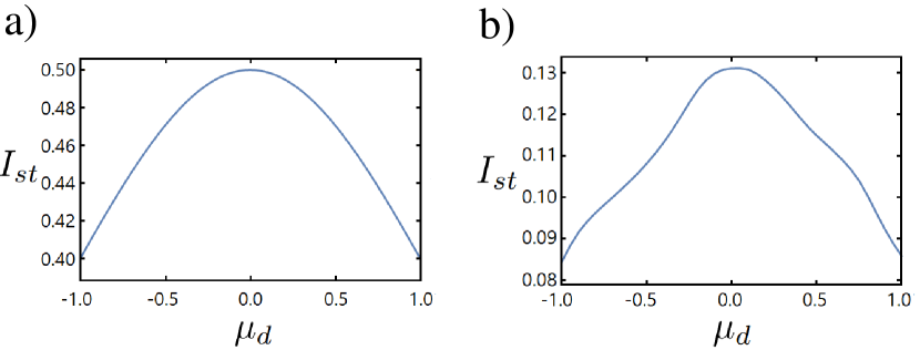
Figure 13:
a: $I_{\rm st}$ as a function of $\mu_{d}$ computed in an HM with $L=19$, $J=1$, $\mu_{\rm eff}=0$, and $U=0$, in the large bias limit with $\Gamma_{1}=\gamma_{L}=g=2$, with a site corresponding to the Hamiltonian in Eq.(24);
b: The same as in a), but with $U=1.5$.

We now discuss the case of a bond impurity, which we symmetrically locate in the middle of an even-$L$ chain. Specifically, we use the impurity Hamiltonian $H_{\rm bond}$, given by

$$H_{\rm bond}=-\delta J\>\{c_{\frac{L}{2}}^{\dagger}c_{\frac{L}{2}+1}+c_{\frac{L}{2}+1}^{\dagger}c_{\frac{L}{2}}\}\>\>\>\>.$$ (25)

In Fig.14a), we plot $n_{{\rm st},j}$, computed in an 1HM with $L=20$, $J=1$, $\mu_{\rm eff}=0$, and $U=0$, in the large bias limit with $\Gamma_{1}=\gamma_{L}=g=2$, with the bond impurity symmetrically located between sites $\bar{j}=10$ and $\bar{j}+1=11$, at various values of the total bond strength $J_{d}=J+\delta J$ (see figure caption for details). At variance, to evidence the effects of the bulk interaction, in Fig.14b) we again show the NESS particle density in real space as a function of the position in the chain, computed for the same parameters as in the left-hand plot, except that now we fix $J_{d}=0.5$ and vary $U$ from plot to plot (see figure caption for details).

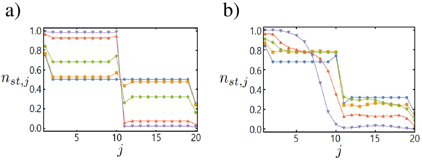
Figure 14:
a: $n_{{\rm st},j}$ computed in an 1HM with $L=20$, $J=1$, $\mu_{\rm eff}=0$, and $U=0$, in the large bias limit with $\Gamma_{1}=\gamma_{L}=g=2$, with the bond impurity symmetrically located between sites $\bar{j}=10$ and $\bar{j}+1=11$, at $J_{d}=1.0$ (blue dots, blue interpolating curve), $J_{d}=0.8$ (orange squares, orange interpolating curve), $J_{d}=0.5$ (green rhombi, green interpolating curve), $J_{d}=0.2$ (red upward pointing triangles, red interpolating curve), and $J_{d}=0.1$ (purple downward pointing triangles, purple interpolating curve);
b: $n_{{\rm st},j}$ computed in an HM with $L=20$, $J=1$, $\mu_{\rm eff}=0$, in the large bias limit with $\Gamma_{1}=\gamma_{L}=g=2$, with the bond impurity symmetrically located between sites $\bar{j}=10$ and $\bar{j}+1=11$, at $J_{d}=0.5$, and with (blue dots, blue interpolating curve), $U=0.5$ (orange squares, orange interpolating curve), $U=1.0$ (green rhombi, green interpolating curve), $U=1.5$ (red upward pointing triangles, red interpolating curve), and $U=2.0$ (purple downward pointing triangles, purple interpolating curve).

Aside for quantitative differences, the plots in Fig.14 exhibit the same behavior as the ones in Fig.12. Thus, we conclude that, changing the type of isolated impurity in the chain, does not substantially affect the charge-density distribution in the NESS. Again, the result in Fig.14 is pertinently complemented by looking at $I_{\rm st}$, as a function of $J_{d}$. Repeating the analysis we have performed above in the case of a site impurity, in Fig.15 we plot $I_{\rm st}$ as a function of $J_{d}$ in the case $U=0$ (Fig.15a)), and for $U=1.5$ (Fig.15b)). Also, in Fig.11b) we draw plots of $I_{\rm st}$ as a function of $L$ up to $L\sim 100$ and for various values of $\frac{U}{J}$, finding results qualitatively similar to the ones we display in Fig.11a) for the site impurity.

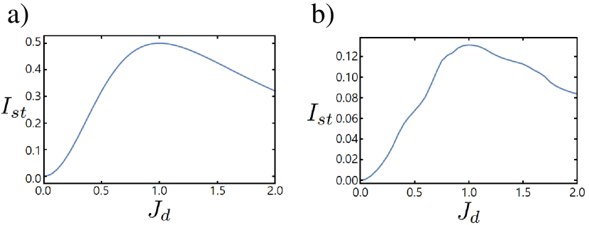
Figure 15: a: $I_{\rm st}$ as a function of $J_{d}$ computed in an HM with $L=20$, $J=1$, $\mu_{\rm eff}=0$, and $U=0$, in the large bias limit with $\Gamma_{1}=\gamma_{L}=g=2$, with the bond impurity corresponding to the Hamiltonian in Eq.(25). b; The same as in a), but with $U=1.5$.

Basically, the same conclusions we reach in the case of a site impurity apply to $I_{\rm st}$ in the NESS in the presence of a bond impurity. The main difference, due to the “directional” nature of the bond impurity, compared to the site impurity, is that, in this case, the current is not symmetrically distributed about $J_{d}=1.0$ (corresponding to $\delta J=0$).

To summarize, we have provided evidences that a single impurity in the chain (either a site impurity, or a bond impurity) does not qualitatively affect the NESS with respect to what happens in a homogeneous 1HM. So, we expect no relevant modifications in the location and in the characteristics of the OWP with respect to the one emerging in the homogeneous chain.

In the next section, we extend this analysis to the case of a finite density of impurities in the chain (quenched disorder), particularly focusing on how, and to what extent, the emergence of the OWP in the system in the large bias limit is affected by the disorder.

VI NESS and OWP in the presence of a finite density of impurities

In the previous Section we have argued how the OWP should not be substantially affected by a single localized defect in the chain. At variance, as it is well estabilished how a finite amount of disorder affects the transport properties of the system in the NESS Žnidarič et al. (2016); Mendoza-Arenas et al. (2019); Schulz et al. (2018), we expect that it affects the OWP, as well, in principle even determining it disappearance, in the strong disorder limit. Motivated by these observations, in this Section we extend the analysis of the effects of the impurities by considering the case in which a finite density of impurities is present in the system, by particularly focusing onto the effects of disorder on the OWP.

To introduce disorder in the 1HM we can, e.g., randomize the chemical potential $\mu$ and/or the bond electron hopping strength $J$ and/or the interaction strength $U$, et cetera. Yet, apart for differences in the structure of the final phase that are realized in the system as a consequence of the disorder (see, for instance, Ref.[Doty and Fisher, 1992] for a comprehensive discussion about this point), disorder is, in general, expected to substantially affect the transport properties of the system, especially in lower dimensions Abrahams et al. (1979). Taking this into account and also to be able to make a systematic comparison with the results of Ref.[Žnidarič et al., 2016], in the following we focus onto a model with a random chemical potential, corresponding to a random applied field in the $z$-direction in the $XXZ$ spin chain discussed in Ref.[Žnidarič et al., 2016]. Technically, we realize this by setting

$$\mu_{\rm eff}\to\mu_{j}=\bar{\mu}+\delta\mu_{j}\;\;\;\;,$$ (26)

with $j=1,...,L$ and with $\{\delta\mu_{j}\}$ independent random variables described by a probability distribution $P[\{\delta\mu_{j}\}]=\prod_{j=1}^{\ell}p(\delta\mu_{j})$. Specifically, we choose $p(\delta\mu)$ to be the probability distribution for $\delta\mu$ with average $\bar{\delta\mu}=\int\>d\delta\mu\>\delta\mu p(\delta\mu)=0$, and with variance $\sigma_{\mu}^{2}=\int\>d\delta\mu\>\delta\mu^{2}p(\delta\mu)$. As a result, we obtain

$$\overline{\delta\mu_{j}} = \int\>\prod_{r=1}^{\ell}d\delta\mu_{r}\>P[\{\delta\mu_{r}\}]\delta\mu_{j}=0$$ (27)

$$\overline{\delta\mu_{i}\delta\mu_{j}} = \int\>\prod_{r=1}^{\ell}d\delta\mu_{r}\>P[\{\delta\mu_{r}\}]\delta\mu_{i}\delta\mu_{j}=\sigma_{\mu}^{2}\delta_{i,j}\>\>\>\>,$$

with $\overline{O[\{\delta\mu_{j}\}]}$ denoting the ensemble average of a generic functional of $\{\delta\mu_{j}\}$ with respect to the probability distribution $P[\{\delta\mu_{j}\}]$. We use the uniform probability distribution given by

$$p(\delta\mu)\>=\>\Biggl{\{}\begin{array}[]{l}\frac{1}{2\sqrt{3}\sigma_{\mu}}\;\;,\;{\rm for}\>-\sqrt{3}\sigma_{\mu}\leq V\leq\sqrt{3}\sigma_{\mu}\\ 0\>\>,\>{\rm otherwise}\end{array}\>\>\>\>.$$ (28)

Having assumed the probability distribution in Eq.(28), we use it to estimate the disorder-averaged current distribution at given values of $\sigma_{\mu}$ and $U$. In particular, having stated that, in the “clean” limit and at large bias, the 1HM is insulating for $\frac{U}{J}>2$, in the following we focus onto the interval of values $0\leq\frac{U}{J}\leq 2$. As for what concerns $\sigma_{\mu}$, we restrict ourselves to the interval $0\leq\frac{\sigma_{\mu}}{J}\leq 1$ which, as we show in the following, for the specific system we focus on, is enough to trigger a transition to an insulating phase for any value of $U$, given the values of the system parameters that we consider here.

We report in Fig.16 our main result for $\bar{I}_{\rm st}$ in the $\sigma_{\mu}-U$ plane, obtained by ensemble averaging $I_{\rm st}$ derived in a 1HM with $L=20$-sites with $J=1$, $\bar{\mu}=0$, in the large bias limit with $\Gamma_{1}=\gamma_{L}=g=2$, over $N=50$ realizations of the disorder. As a main remark, we note an over-all consistency with the analogous diagram reported in Fig.1 of Ref.[Brenes et al., 2018], despite the differences in the parameters of the systems considered in the two cases.

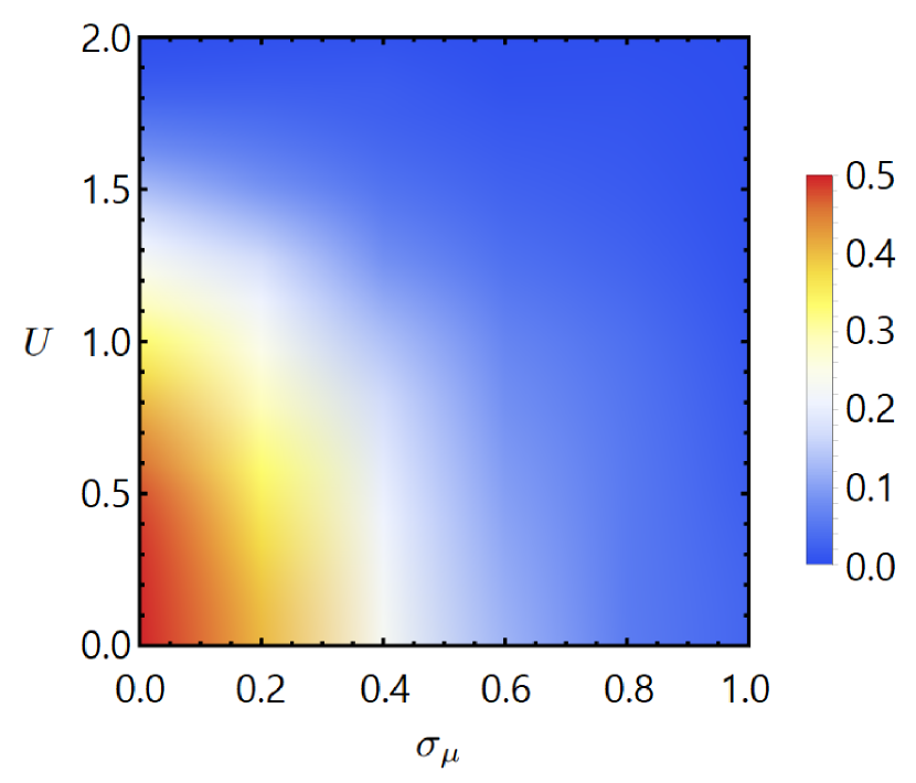
Figure 16: $\bar{I}_{\rm st}$ in the $\sigma_{\mu}-U$ plane, obtained by ensemble averaging $I_{\rm st}$ derived in 1HM with $L=20$-sites with $J=1$, $\bar{\mu}=0$, in the large bias limit with $\Gamma_{1}=\gamma_{L}=g=2$, over $N=50$ realizations of the disorder. The color code for the value of $\bar{I}_{\rm st}$ is summarized in the side vertical bar.

As expected, the larger is $\sigma_{\mu}$ (at fixed $U$), the lower is the values of $U$ at which the transition from the conducting to the insulating phase takes place. This basically gives rise to a “critical line” in the $\sigma_{\mu}-U$ plan, with a shading of the transition line due to the disorder-triggered nature of the phase transition. Indeed, the conductor to insulator phase transition can be pictured as a proliferation of the “kinks” localized at each defect in the chain, which eventually, at a strong enough value of $\sigma_{\mu}$, coalesce into a single larger kink distributed throughout the whole chain. When this happens, the conduction gets blocked (similarly to what happens in the clean system for $\frac{U}{J}>2$). So, the mechanism appears to be analogous to what happens at the Griffiths phase transition in disordered system, with a similar effect on the spreading of the critical line between the two phases Altland and Zirnbauer (1997); Motrunich et al. (2001); Nava et al. (2017). To highlight the combined effect of a finite $U$ and a finite $\sigma_{\mu}$ in triggering the transition to the insulating phase, in Fig.17 we plot $\bar{I}_{\rm st}$ along two cuts of Fig.16, respectively corresponding to the segment $\sigma_{\mu}=0.2,0\leq U\leq 2$ (Fig.17a)) and to $U=0.5,0\leq\sigma_{\mu}\leq 1$ (Fig.17b)), computed in an $L=20$ chain with $J=1$, $\bar{\mu}=0$, in the large bias limit with $\Gamma_{1}=\gamma_{L}=g=2$. In both cases, we clearly see the transition from the conducting to the insulating regime. Apparently, following the analysis of Ref.[Žnidarič et al., 2016], our result implies that the localization length of the system, $L_{*}$, (which is expected to be a function of both $\sigma_{\mu}$ and $U$), is always $\leq L$, so to allow for the disorder-induced transition (in fact a crossover) to the insulating phase in the $L=20$ chain.

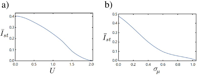
Figure 17:
a: $\bar{I}_{\rm st}$ computed in an $L=20$ chain with $J=1$, $\bar{\mu}=0$ in the large-bias limit with $\Gamma_{1}=\gamma_{L}=g=2$. along the cut of Fig.16 corresponding to the segment $\sigma_{\mu}=0.2,0\leq U\leq 2$ and to $U=0.5,0\leq\sigma_{\mu}\leq 1$;
b: $\bar{I}_{\rm st}$ computed in the same system as in a) and evaluated along the cut of Fig.16 corresponding to the segment $U=0.5,0\leq\sigma_{\mu}\leq 1$.

Having checked the consistency of our results with the phase diagram of Ref.[Žnidarič et al., 2016], we now discuss the effects of the disorder on the OWP. To do so, we first move along the horizontal line of Fig.16 corresponding to $U=0$. Repeating the analysis of Section III in the presence of disorder, we compute $\bar{I}_{\rm st}$ as a function of $f$ in a 1HM with $L=20$-sites with $J=1$, $\bar{\mu}=0$, $U=0$, with $\Gamma_{1}=\gamma_{L}=g=2$, by ensemble averaging over $N=50$ realizations of the disorder and for different values of $\sigma_{\mu}$ (Fig.18a)), as well as at nonequilibrium, as a function of $g$, in the same system and using the same procedure, again for different values of $\sigma_{\mu}$ (Fig.18b)).

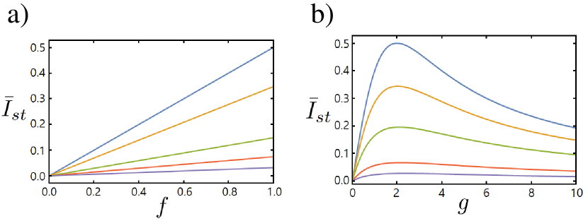
Figure 18:
a: $\bar{I}_{\rm st}$ as a function of $f$ in a 1HM with $L=20$-sites with $J=1$, $\bar{\mu}=0$, $U=0$, and $\Gamma_{1}=\gamma_{L}=g=2$, computed by ensemble averaging over $N=50$ realizations of the disorder for different values of $\sigma_{\mu}$;
b: $\bar{I}_{\rm st}$ as a function of $g$ in a 1HM $L=20$-sites with $J=1$, $\bar{\mu}=0$, $U=0$, taken to the large bias limit with $\Gamma_{1}=\gamma_{L}=g=2$, computed by ensemble averaging over $N=50$ realizations of the disorder, again for different values of $\sigma_{\mu}$. In both panels we have set: $\sigma_{\mu}=0.0$ (blue line), $\sigma_{\mu}=0.5$ (yellow line), $\sigma_{\mu}=1.0$ (green line), $\sigma_{m}u=1.5$ (red line), and $\sigma_{\mu}=2.0$ (purple line).

Remarkably, from Fig.18b), we see that a limited amount of disorder does not spoil our result that the OWP point in $I_{\rm st}$ as a function of $g$ appears in the chain when it is taken out of equilibrium even when $U=0$. Eventually, a strong disorder washes out the OWP which, from Fig.18a), we find to happen simultaneously with a reduction of $\bar{I}_{\rm st}$ to 0, that is, to the phase transition from the conducting to the insulating phase.

Consistently with our result that a limited amount of disorder does not wash out the OWP at $U=0$, we expect that the same happens at $U>0$. To check this guess, in Fig.19 we plot $\bar{I}_{\rm st}$ computed in the same system as the one we used to derive Fig.18, but choosing $U=1.5$. As expected, disorder does not substantially affect the OWP, which proves to be pretty stable against the presence of impurities in the chain, both in the noninteracting case, as well as for a finite value of $U$.

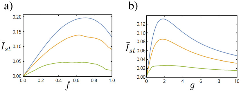
Figure 19:
a: $\bar{I}_{\rm st}$ as a function of $f$ in a 1HM at equilibrium with $L=20$-sites with $J=1$, $\bar{\mu}=0$, $U=1.5$, and $\Gamma_{1}=\gamma_{L}=g=2$, computed by ensemble averaging over $N=50$ realizations of the disorder for different values of $\sigma_{\mu}$;
b: $\bar{I}_{\rm st}$ as a function of $g$ in a 1HM $L=20$-sites with $J=1$, $\bar{\mu}=0$, $U=1.5$, taken to the large bias limit with $\Gamma_{1}=\gamma_{L}=g=2$, computed by ensemble averaging over $N=50$ realizations of the disorder, again for different values of $\sigma_{\mu}$. In both panels we have set: $\sigma_{\mu}=0.0$ (blue line), $\sigma_{\mu}=0.25$ (yellow line), $\sigma_{\mu}=0.5$ (green line).

Our sampling analysis, combined with the over-all phase diagram of the disordered 1HM in the $\sigma_{\mu}-U$-plane in Fig.16, let us infer that, at any point of the phase diagram characterized by a finite value of the ensemble averaged $\bar{I}_{\rm st}$, it is always possible, in the large bias limit, to tune the system at the OWP by pertinently operating over the parameters $\Gamma_{1},\gamma_{L},g$ and $f$. This result, together with our finding that tuning $g$ allows for recovering the OWP even when $U=0$, shows that the emergence of the OWP itself and the corresponding onset of a negative differential conductivity in the chain, are pretty universal features, robust against both the electronic interaction as well as the disorder in the chain.

VII Conclusions

Using the Lindblad equation approach we have discussed the main features of the NESS arising in an interacting one-dimensional electronic chain connected to two reservoirs in the large bias limit. To do so, we have characterized the NESS by synoptically monitoring both the stationary current $I_{\rm st}$ and the stationary charge distribution in real space, $n_{{\rm st},j}$, characterizing the NESS. In the noninteracting case, we were able to do so within a fully analytical approach, by providing explicit formulas for $I_{\rm st}$ and $n_{{\rm st},j}$ in the NESS.

In the presence of a nonzero electronic interaction, we have resorted to a MF approach to the interaction, which allowed us to perform a systematic characterization of the NESS as a function of the bias between the reservoirs, of the strength of the couplings between the chain and the reservoirs, of the bulk interaction in the chain and, eventually, when breaking the chain homogeneity with an isolated impurity, as a function of the type and of the strength of the impurity potential. Finally, we have introduced a finite density of impurities in the chain to discuss how the NESS depends on the amount of quenched disorder, as well.

Our analysis allowed us to characterize the emergence of an OWP in the multi-parameter space, at which $I_{\rm st}$ is maximized with respect to the values of the various parameters. Eventually, we showed that the OWP is robust against the presence of a limited amount of disorder in the chain, while a strong enough disorder washes it out, by triggering, at the same time, a disorder-induced transition from a conducting to an insulating NESS.

The importance of our results is strictly related to the importance of both understanding the nature of the OWP and, after that, of tuning a device at the OWP in a large number of cases of physical interest.

Because of its simplicity, combined with its reliability, which we checked by comparing our results to the ones available in the literature about LE approach to nonequilibrium quantum systems, we plan to extend our approach to, e.g., look for novel phases/phase transitions arising in the phase diagram of junctions of interacting fermionic systems Oshikawa et al. (2006); Hou and Chamon (2008); Giuliano and Affleck (2019); Kane et al. (2020); Giuliano and Nava (2015); Giuliano et al. (2020a) and/or spin chains Tsvelik (2013); Giuliano et al. (2016); Giuliano et al. (2020b), or to define systematical optimization procedure for the parameters determining the working point of a quantum device, and so on.

Acknowledgements – We gratefully thank D. Rossini for insightful discussions.

A. N. was financially supported by POR Calabria FESR-FSE 2014/2020 - Linea B) Azione 10.5.12, grant no. A.5.1. D. G. and M. R. acknowledge financial support from Italy’s MIUR PRIN projects TOP-SPIN (Grant No. PRIN 20177SL7HC).

Appendix A Variational approach to the stationary current and to the real space charge distribution in the nonequilibrium stationary state

In this appendix we present a simple variational approach to the “kink confinement”, and to the corresponding conductor-to-insulator phase transition, which we found in the 1HM connected to two reservoirs, in the large bias limit. To do so, we first of all remark that, via the (inverse) Jordan-Wigner transformation, the Hamiltonian in Eq.(21) at $\mu_{\rm eff}=0$ is mapped onto the Hamiltonian for the $XXZ$ spin chain in a zero magnetic field, $H_{XXZ}$, given by

$$H_{XXZ}=-J\sum_{j=1}^{L-1}\{S_{j}^{+}S_{j+1}^{-}+S_{j}^{-}S_{j+1}^{+}\}+J\Delta\sum_{j=1}^{L-1}S_{j}^{z}S_{j+1}^{z}\>\>\>\;,$$ (29)

with $S^{+}_{j}=c_{j}^{\dagger}\>e^{i\pi\sum_{t=1}^{j-1}c_{t}^{\dagger}c_{t}}$ and $S_{j}^{z}=c_{j}^{\dagger}c_{j}-\frac{1}{2}$. In particular, $\frac{U}{J}<(>)2$ in the 1HM corresponds to $\Delta<(>)1$ in $H_{XXZ}$ in Eq.(29). Along the correspondence between operators in the 1HM and in the $XXZ$ Hamiltonian, we find that the charge density at site $j$ and the current density through the link between $j$ and $j+1$ in the former model are respectively expressed in terms of operators in the latter model as

$$n_{j} = S_{j}^{z}+\frac{1}{2}$$

$$I_{j,j+1} = -iJ\{S_{j}^{+}S_{j+1}^{-}-S_{j+1}^{+}S_{j}^{-}\}\>\>\>\>.$$ (30)

Once the reservoirs have driven the system towards the NESS, the current must be uniform throughout the chain and equal to $I_{\rm st}$. At the same time, setting $n_{{\rm st},j}=\langle n_{j}\rangle_{\rm st}$, where $\langle\ldots\rangle_{\rm st}$ denotes averaging within the NESS, in the large bias regime $I_{\rm st}$ is related to both $n_{{\rm st},1}$ and $n_{{\rm st},j}$ through the relations

$$I_{\rm st} = \Gamma_{1}\>[1-n_{{\rm st},1}]=\Gamma_{1}\left\{\frac{1}{2}-\langle S_{1}^{z}\rangle_{\rm st}\right\}$$

$$I_{\rm st} = \gamma_{L}\>n_{{\rm st},L}=\gamma_{L}\left\{\frac{1}{2}+\langle S_{L}^{z}\rangle_{\rm st}\right\}\>\>\>\>,$$ (31)

with the relation with the average local magnetization in the $XXZ$ model explicitly evidenced. Choosing, as we have done in Section IV, $\Gamma_{1}=\gamma_{L}$, implies therefore $\langle S_{1}^{z}\rangle_{\rm st}=-\langle S_{L}^{z}\rangle_{\rm st}\equiv m_{\rm bou}$. Resorting to the $XXZ$ spin chain framework we can therefore adapt the semiclassical approach introduced in Ref.[Alcaraz et al., 1995] to discuss the kink dynamics for $\Delta\geq 1$ to a generic value of $\Delta$ and, in particular, to the case $|\Delta|\leq 1$, which is the one we focus on in Section IV.

Following Ref.[Alcaraz et al., 1995], we treat the spin operators in $H_{XXZ}$ as classical variables, for which we make an appropriate variational ansatz. Computing the energy of the corresponding state using Eq.(29) supplemented with the constraints implied by Eqs.(31) and minimizing the corresponding result with respect to the variational parameters, we find out how the kink solution varies as a function of the $I_{\rm st}$ as well as of $U$. Letting $\vec{\cal S}_{j}$ be our variational ansatz for the spin operator at site $j$ (to be eventually identified with $\langle\vec{S}_{j}\rangle_{\rm st}$), we set (assuming that, at the boundaries, the spin are fully polarized in the $z$-direction, due to the coupling with the reservoirs)

$$\vec{\cal S}_{j}\equiv\left[\begin{array}[]{c}{\cal S}_{j}^{x}\\ {\cal S}_{j}^{y}\\ {\cal S}_{j}^{z}\end{array}\right]=\left[\begin{array}[]{c}\cos(\varphi_{j})\sin(\vartheta_{j})\\ \sin(\varphi_{j})\sin(\vartheta_{j})\\ \cos(\vartheta_{j})\end{array}\right]\>\>\>\>,$$ (32)

with $\vartheta_{j},\varphi_{j}$ being smooth functions of the real space variable, so to enable us to treat them as smooth functions of a continuous coordinate variable $x$. In order to choose ${\cal S}_{j}^{z}=\cos(\vartheta_{j})$ so to match the density profiles in Fig.8, we make a “minimal” variational ansatz, that is, we fit the magnetization profile with a trial function depending on one variational parameter only. As we discuss below, though being a pretty crude approximation, our variational ansatz is apparently good enough to allow for qualitatively recovering all the key features highlighted in Sections III,IV. Specifically, we choose our trial function so that (resorting to a the continuous variable $x$)

$${\cal S}_{j}^{z} \to \frac{1}{2}\>\left\{\frac{1}{1+e^{(x-\ell)}}-\frac{1}{1+e^{(L-x-\ell)}}\right\}$$ (33)

$$\equiv \frac{1}{2}\>\cos(\vartheta(x=aj))\>\>\>\>,$$

with $a$ being the lattice step and $L$ being the length of the chain. The only variational parameter entering the function in Eq.(33) is the length scale $\ell$.

To variationally determine $\ell$, we estimate the energy for the Hamiltonian in Eq.(29) corresponding to our variational solution in Eq.(33), ${\cal E}[\ell]$, by using the MF result of Ref.[Misguich et al., 2019]. Doing so, we set

$${\cal E}[\ell]\approx\frac{J}{2}\int_{0}^{L}dx\left\{\left(\frac{d\vec{\cal S}}{dx}\right)^{2}-2(\Delta-1)({\cal S}^{z})^{2}\right\}$$ (34)

$$= \frac{J}{2}\int_{0}^{L}dx\biggl{\{}\left(\frac{d\vartheta(x)}{dx}\right)^{2}+\sin^{2}(\vartheta(x))\left(\frac{d\varphi(x)}{dx}\right)^{2}$$

$$- 2(\Delta-1)\cos^{2}(\vartheta(x))\biggr{\}}\>\>\>\>.$$

In addition to $\vartheta(x)$, ${\cal E}[\ell]$ also depends on $\varphi(x)$. To determine this latter function we employ the current conservation within the NESS, which implies that $I_{\rm st}$ is the same independently of the position in the chain. Within MF approximation Misguich et al. (2019), we get $I_{\rm st}=J\>\sin^{2}(\vartheta(x))\frac{d\varphi(x)}{dx}$. Therefore, we obtain

$$I_{\rm st} \approx J\>\sin^{2}(\vartheta(x))\frac{d\varphi(x)}{dx}$$ (35)

$$\Rightarrow \frac{d\varphi(x)}{dx}=\frac{I_{\rm st}}{J}\>\sin^{-2}(\vartheta(x))\>\>\>\>.$$

Using Eq.(35), we may rewrite Eq.(34) as

$${\cal E}[\ell] = \frac{J}{2}\int_{0}^{L}dx\biggl{\{}\left(\frac{d\vartheta(x)}{dx}\right)^{2}+\left(\frac{I_{\rm st}}{J\sin^{2}(\vartheta(x))}\right)^{2}$$ (36)

$$- 2(\Delta-1)\cos^{2}(\vartheta(x))\biggr{\}}\>\>\>\>.$$

To explicitly put the right-hand side of Eq.(36) in a form depending on $\ell$ only, we recall that, from Eqs.(31), we obtain

$$I_{\rm st}=\Gamma_{1}\>\left\{\frac{1}{2}-m_{\rm bou}\right\}=\Gamma_{1}\>\left\{\frac{1}{2}-\frac{\cos(\vartheta(0))}{2}\right\}\>\>\>\>.$$ (37)

To recover the results of Figs.7,8, we minimized, with respect to $\ell$, ${\cal E}[\ell]$ computed at fixed $\Gamma_{1}=\gamma_{L}=g=2$ and for a given $\Delta$. Once we had estimated in this way the parameter in the trial function of Eq.(33), we computed $n_{{\rm st}}$ throughout the chain as a function of $U$, as well as $m_{\rm bou}$. Knowing $m_{\rm bou}$, we eventually used Eq.(37) to compute $I_{\rm st}$ as a function of $U$. In Fig.20 we draw $I_{\rm sp}$ computed within our variational approach as a function of $U$ in the large bias limit with $\Gamma_{1}=\gamma_{L}=g=2$ (blue dots), together with the analogous quantity computed using the numerical approach of Section IV (orange squares), in an $L=20$ chain with $J=1$ and $\mu_{\rm eff}=0$. While, possibly due to our oversimplified choice for the trial wavefunction, there is a rather weak quantitative agreement between the points, we believe that the qualitative agreement is satisfactory enough and witnesses the reliability of our method: indeed, we see that in both cases $I_{\rm st}$ monotonically decreases on increasing $U$ from 0 to positive values and eventually becomes 0 as soon as $U\geq 2$, which is also consistent with Refs.[Benenti et al., 2009b, a]. Moreover, as pointed out in Ref.[Misguich et al., 2019], the effective continuum energy functional in Eq.(34) is expected to be mostly reliable for $\Delta\sim 1$, corresponding to $\frac{U}{J}\sim 2$ in our model, where, indeed, the agreement between the two plots is pretty good, even quantitatively.

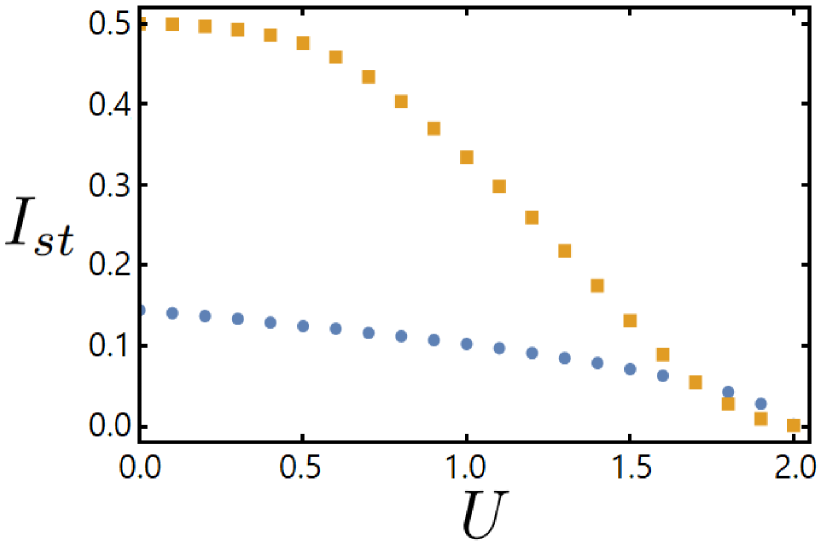
Figure 20: $I_{\rm st}$ as a function of $U$ computed within our variational approach in an $L=20$ chain with $J=1$ and $\mu_{\rm eff}=0$, in the large bias limit with $\Gamma_{1}=\gamma_{L}=g=2$ (blue dots), and using the numerical approach of Section IV with the same values of the system parameters (orange squares).

In Fig.21, we plot $n_{\rm st}$ within the NESS as a function of $x$ computed within the variational approach. Apparently, using the variational approach allows us for recovering a pretty good agreement with the trend evidenced in Fig.8: as long as the system supports a nonzero $I_{\rm st}$, $n_{\rm st}$ is flat at $n_{\rm st}=\frac{1}{2}$ throughout the middle part of the chain, with a respectively upward and downward turn close to the endpoints of the chain, that are required to match $n_{{\rm st},1}$ and $n_{{\rm st},L}$ as determined by the constancy of $I_{\rm st}$. On increasing $U$, the extent of the flat region gets reduced, till the region shrinks at $U=2$, where $n_{\rm st}$ takes a “kink-like” profile, with a corresponding blocking of the current transport ($I_{\rm st}=0$), for $U>2$ Benenti et al. (2009a, b).

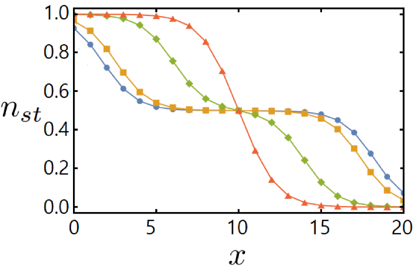
Figure 21: $n_{\rm st}$ as a function of $x$ computed within our variational approach in an $L=20$ chain with $J=1$ and $\mu_{\rm eff}=0$, in the large bias limit with $\Gamma_{1}=\gamma_{L}=g=2$, and with $U=0$ (blue circles - blue interpolating curve), $U=1.5$ (orange rhombi - orange interpolating curve), $U=1.9$ (green squares - green interpolating curve), and $U=2.1$ (red triangles - red interpolating curve). Note that, to account for errors induced by the crude approximations in our choice of the trial function, the values of $U$ are slightly larger than what is expected from the numerical results of Section IV. Yet, the qualitative agreement with the numerical results is pretty good.

Before concluding this Appendix, it is worth mentioning that, by means of a simple extension of the crude variational approach we discussed above, we are able to catch the remarkable emergence of an OWP in the plot of $I_{\rm st}$ as a function of $\Gamma_{1}=\gamma_{L}=g$, derived in the fully nonequilibrium limit $f=1$ and in the noninteracting case $U=0$. In fact, while, consistently with Refs.[Benenti et al., 2009a], in Section IV we find no OWP when plotting $I_{\rm st}$ as a function of $f$ for $\Gamma_{1}=\gamma_{L}=g$ and for $U=0$, instead, we do find the OWP in the plot of $I_{\rm st}$ as a function of $\Gamma_{1}=\gamma_{L}=g$, as we show throughout Section III, as well as in Fig.9b). To recover the OWP for $U=0$ we used the energy functional in Eq.(34) with $\Delta=0$ and a variational function obtained by applying a rigid translation by $x_{0}$ to the function of Eq.(33), that is

$${\cal S}_{j}^{z} \to \frac{1}{2}\>\left\{\frac{1}{1+e^{(x-x_{0}-\ell)}}-\frac{1}{1+e^{(L-x+x_{0}-\ell)}}\right\}$$ (38)

$$\equiv \frac{1}{2}\>\cos(\vartheta(x=aj))\>\>\>\>.$$

We determine the parameters $\ell$ and $x_{0}$ by imposing the constraint that the values of $m_{{\rm bou},1},m_{{\rm bou},L}$ obtained from Eq.(38) are consistent with Eq.(31). Doing so, we obtain the plot in Fig.22, where we draw $I_{\rm st}$ computed using the variational approach at $J=1$, $L=20$ and $U=0$, at large bias, as a function of $\gamma_{L}=\Gamma_{1}=g$ (blue curve) and as a function of $\gamma_{L}=g$ at $\Gamma_{1}=2$ (orange curve). In both cases the location of the OWP is consistent with the results of Section III, though, due to the pretty crude approximations behind our variational approach, the calculated value of $I_{\rm st}$ is lower than the one numerically computed by a factor of 4. Yet, this is consistent with the analogous reduction of $I_{\rm st}$ vs. $U$ in Fig.20 as $U\to 0$.

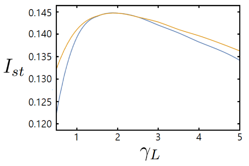
Figure 22: $I_{\rm st}$ computed using the variational approach at $J=1$, $L=20$ and $U=0$, at large bias, as a function of $\gamma_{L}=\Gamma_{1}=g$ (blue curve) and as a function of $\gamma_{L}=g$ at $\Gamma_{1}=2$ (orange curve). The reduction by a factor of 4 with respect to the numerical results of Section III is consistent with the analogous reduction of $I_{\rm st}$ vs. $U$ in Fig.20 as $U\to 0$.

References

- Mello and Kumar (2004) P. A. Mello and N. Kumar, Quantum Transport in Mesoscopic Systems (Oxford University Press, Oxford, U.K., 2004).
- Prosen (2008) T. Prosen, New Journal of Physics 10, 043026 (2008).
- Henrich et al. (2007) M. J. Henrich, G. Mahler, and M. Michel, Phys. Rev. E 75, 051118 (2007).
- Burgarth and Giovannetti (2007) D. Burgarth and V. Giovannetti, Phys. Rev. Lett. 99, 100501 (2007).
- You et al. (2000) J. Q. You, C.-H. Lam, and H. Z. Zheng, Phys. Rev. B 62, 1978 (2000).
- Datta (1993) S. Datta, Keldysh Formalism and the Landauer Approach (Springer US, Boston, MA, 1993), pp. 299–331, ISBN 978-1-4899-2415-5.
- Gorini et al. (1976) V. Gorini, A. Kossakowski, and E. C. G. Sudarshan, Journal of Mathematical Physics 17, 821 (1976).
- Lindblad (1976) G. Lindblad, Communications in Mathematical Physics 48, 119 (1976).
- Schoeller (2009) H. Schoeller, The European Physical Journal Special Topics 168, 179–266 (2009).
- Berges and Mesterházy (2012) J. Berges and D. Mesterházy, Nuclear Physics B - Proceedings Supplements 228, 37 (2012).
- Jakobs et al. (2007) S. G. Jakobs, V. Meden, and H. Schoeller, Phys. Rev. Lett. 99, 150603 (2007).
- Gutman et al. (2010) D. B. Gutman, Y. Gefen, and A. D. Mirlin, Phys. Rev. B 81, 085436 (2010).
- Ngo Dinh et al. (2012) S. Ngo Dinh, D. A. Bagrets, and A. D. Mirlin, Annals of Physics 327, 2794 (2012).
- Levkivskyi (2012) I. Levkivskyi, Equilibrium and Non-Equilibrium Bosonization (Springer Berlin Heidelberg, Berlin, Heidelberg, 2012), pp. 41–53.
- Breuer and Petruccione (2002) H.-P. Breuer and F. Petruccione, The Theory of Open Quantum Systems (Oxford University Press, 2002).
- Weiss (1993) U. Weiss, Quantum Dissipative Systems (WORLD SCIENTIFIC, Singapore, 1993).
- Carlo et al. (2003) G. G. Carlo, G. Benenti, and G. Casati, Phys. Rev. Lett. 91, 257903 (2003).
- Carlo et al. (2004) G. G. Carlo, G. Benenti, G. Casati, and C. Mejía-Monasterio, Phys. Rev. A 69, 062317 (2004).
- Benenti et al. (2009a) G. Benenti, G. Casati, T. Prosen, D. Rossini, and M. Žnidarič, Phys. Rev. B 80, 035110 (2009a).
- Vidal (2003) G. Vidal, Phys. Rev. Lett. 91, 147902 (2003).
- Vidal (2004) G. Vidal, Phys. Rev. Lett. 93, 040502 (2004).
- White and Feiguin (2004) S. R. White and A. E. Feiguin, Phys. Rev. Lett. 93, 076401 (2004).
- Brenes et al. (2018) M. Brenes, E. Mascarenhas, M. Rigol, and J. Goold, Phys. Rev. B 98, 235128 (2018).
- Langer et al. (2009) S. Langer, F. Heidrich-Meisner, J. Gemmer, I. P. McCulloch, and U. Schollwöck, Phys. Rev. B 79, 214409 (2009).
- Benenti et al. (2009b) G. Benenti, G. Casati, T. Prosen, and D. Rossini, EPL (Europhysics Letters) 85, 37001 (2009b).
- Sabetta and Misguich (2013) T. Sabetta and G. Misguich, Phys. Rev. B 88, 245114 (2013).
- Sznajd and Becker (2005) J. Sznajd and K. W. Becker, Journal of Physics: Condensed Matter 17, 7359 (2005).
- Thomaz et al. (2014) M. Thomaz, E. Corrêa Silva, and O. Rojas, Condensed Matter Physics 17 (2014).
- Jordan and Wigner (1928) P. Jordan and E. P. Wigner, Zeitschrift für Physik 47, 631 (1928).
- Giuliano and Sodano (2005) D. Giuliano and P. Sodano, Nuclear Physics B 711, 480 (2005).
- Giuliano and Sodano (2008) D. Giuliano and P. Sodano, New Journal of Physics 10, 093023 (2008).
- Giuliano and Sodano (2009) D. Giuliano and P. Sodano, Nuclear Physics B 811, 395 (2009).
- Cirillo et al. (2011) A. Cirillo, M. Mancini, D. Giuliano, and P. Sodano, Nuclear Physics B 852, 235 (2011).
- Karevski and Platini (2009) D. Karevski and T. Platini, Phys. Rev. Lett. 102, 207207 (2009).
- Esaki and Tsu (1970) L. Esaki and R. Tsu, IBM Journal of Research and Development 14, 61 (1970).
- Labouvie et al. (2015) R. Labouvie, B. Santra, S. Heun, S. Wimberger, and H. Ott, Phys. Rev. Lett. 115, 050601 (2015).
- Perrin et al. (2013) M. L. Perrin, C. J. O. Verzijl, C. A. Martin, A. J. Shaikh, R. Eelkema, J. H. van Esch, J. M. van Ruitenbeek, J. M. Thijssen, H. S. J. van der Zant, and D. Dulić, Nature Nanotechnology 8, 282 (2013).
- Pop et al. (2005) E. Pop, D. Mann, J. Cao, Q. Wang, K. Goodson, and H. Dai, Phys. Rev. Lett. 95, 155505 (2005).
- Britnell et al. (2013) L. Britnell, R. V. Gorbachev, A. K. Geim, L. A. Ponomarenko, A. Mishchenko, M. T. Greenaway, T. M. Fromhold, K. S. Novoselov, and L. Eaves, Nature Communications 4, 1794 (2013).
- Thielmann et al. (2005) A. Thielmann, M. H. Hettler, J. König, and G. Schön, Phys. Rev. B 71, 045341 (2005).
- Zazunov et al. (2006) A. Zazunov, D. Feinberg, and T. Martin, Phys. Rev. B 73, 115405 (2006).
- Nazarov and Blanter (2009) Y. V. Nazarov and Y. M. Blanter, Quantum Transport: Introduction to Nanoscience (Cambridge University Press, 2009).
- Barontini et al. (2013) G. Barontini, R. Labouvie, F. Stubenrauch, A. Vogler, V. Guarrera, and H. Ott, Phys. Rev. Lett. 110, 035302 (2013).
- Ortega et al. (2016) A. Ortega, T. Stegmann, and L. Benet, Phys. Rev. E 94, 042102 (2016).
- Conwell (1967) E. M. Conwell, Solid State Pbysics (1967).
- Xu and Teitsworth (2007) H. Xu and S. W. Teitsworth, Phys. Rev. B 76, 235302 (2007).
- Cross and Greenside (2009) M. Cross and H. Greenside, Pattern Formation and Dynamics in Nonequilibrium Systems (Cambridge University Press, 2009).
- Knight and Peterson (1966) B. W. Knight and G. A. Peterson, Phys. Rev. 147, 617 (1966).
- Knight and Peterson (1967) B. W. Knight and G. A. Peterson, Phys. Rev. 155, 393 (1967).
- Qi et al. (2006) Y. Qi, Z.-G. Yu, and M. E. Flatté, Phys. Rev. Lett. 96, 026602 (2006).
- Nagatani (2002) T. Nagatani, Reports on Progress in Physics 65, 1331 (2002).
- Nagatani (1998) T. Nagatani, Phys. Rev. E 58, 4271 (1998).
- Pamplin (1970) B. R. Pamplin, Contemporary Physics 11, 1 (1970).
- Japaridze et al. (2009) G. I. Japaridze, H. Johannesson, and A. Ferraz, Phys. Rev. B 80, 041308 (2009).
- Deng et al. (2000) J. Deng, R. Gaska, M. S. Shur, M. A. Khan, and J. W. Yang, MRS Internet Journal of Nitride Semiconductor Research 5, 355–361 (2000).
- Chiesa et al. (2019) A. Chiesa, E. Macaluso, P. Santini, S. Carretta, and E. Pavarini, Phys. Rev. B 99, 235145 (2019).
- Asadian et al. (2013) A. Asadian, D. Manzano, M. Tiersch, and H. J. Briegel, Phys. Rev. E 87, 012109 (2013).
- Fioravanti and Rossi (2003a) D. Fioravanti and M. Rossi, Journal of High Energy Physics 07, 031 (2003a).
- Fioravanti and Rossi (2003b) D. Fioravanti and M. Rossi, Journal of High Energy Physics 08, 042 (2003b).
- Fioravanti and Rossi (2005) D. Fioravanti and M. Rossi, Journal of High Energy Physics 08, 010 (2005).
- Zotos et al. (1997) X. Zotos, F. Naef, and P. Prelovsek, Phys. Rev. B 55, 11029 (1997).
- Benenti et al. (2013) G. Benenti, G. Casati, and J. Wang, Phys. Rev. Lett. 110, 070604 (2013).
- Rigol (2009) M. Rigol, Phys. Rev. Lett. 103, 100403 (2009).
- Essler et al. (2005) F. H. L. Essler, H. Frahm, F. Göhmann, A. Klümper, and V. E. Korepin, The One-Dimensional Hubbard Model (Cambridge University Press, 2005).
- Pearle (2012) P. Pearle, European Journal of Physics 33, 805 (2012).
- Adler (2000) S. Adler, Physics Letters A 265, 58 (2000).
- Müller and Stace (2017) C. Müller and T. M. Stace, Phys. Rev. A 95, 013847 (2017).
- Nava and Fabrizio (2019) A. Nava and M. Fabrizio, Phys. Rev. B 100, 125102 (2019).
- Bácsi et al. (2020) A. Bácsi, C. P. Moca, and B. Dóra, Phys. Rev. Lett. 124, 136401 (2020).
- Gardiner and Zoller (2000) C. Gardiner and P. Zoller, Quantum Noise (Springer, 2000).
- Guimarães et al. (2016) P. H. Guimarães, G. T. Landi, and M. J. de Oliveira, Phys. Rev. E 94, 032139 (2016).
- Xianlong et al. (2008) G. Xianlong, M. Polini, D. Rainis, M. P. Tosi, and G. Vignale, Phys. Rev. Lett. 101, 206402 (2008).
- Giuliano et al. (2013) D. Giuliano, D. Rossini, P. Sodano, and A. Trombettoni, Phys. Rev. B 87, 035104 (2013).
- Markhof et al. (2018) L. Markhof, B. Sbierski, V. Meden, and C. Karrasch, Phys. Rev. B 97, 235126 (2018).
- Takahashi and Shiroishi (2002) M. Takahashi and M. Shiroishi, Phys. Rev. B 65, 165104 (2002).
- Castro-Alvaredo et al. (2014) O. Castro-Alvaredo, Y. Chen, B. Doyon, and M. Hoogeveen, Journal of Statistical Mechanics: Theory and Experiment 2014, P03011 (2014).
- Mehta and Andrei (2006) P. Mehta and N. Andrei, Phys. Rev. Lett. 96, 216802 (2006).
- Giamarchi (2003) T. Giamarchi, Quantum Physics in One Dimension (Oxford University Press, Oxford, U.K., 2003).
- Mühlbacher and Rabani (2008) L. Mühlbacher and E. Rabani, Phys. Rev. Lett. 100, 176403 (2008).
- Misguich et al. (2019) G. Misguich, N. Pavloff, and V. Pasquier, SciPost Phys. 7, 25 (2019).
- Eggert and Affleck (1992) S. Eggert and I. Affleck, Phys. Rev. B 46, 10866 (1992).
- Sorensen et al. (1993) E. S. Sorensen, S. Eggert, and I. Affleck, Journal of Physics A: Mathematical and General 26, 6757 (1993).
- Kane and Fisher (1992a) C. L. Kane and M. P. A. Fisher, Phys. Rev. Lett. 68, 1220 (1992a).
- Kane and Fisher (1992b) C. L. Kane and M. P. A. Fisher, Phys. Rev. B 46, 15233 (1992b).
- Giuliano et al. (2017) D. Giuliano, P. Sodano, and A. Trombettoni, Phys. Rev. A 96, 033603 (2017).
- Giuliano et al. (2018) D. Giuliano, D. Rossini, and A. Trombettoni, Phys. Rev. B 98, 235164 (2018).
- Žnidarič et al. (2016) M. Žnidarič, A. Scardicchio, and V. K. Varma, Phys. Rev. Lett. 117, 040601 (2016).
- Mendoza-Arenas et al. (2019) J. J. Mendoza-Arenas, M. Žnidarič, V. K. Varma, J. Goold, S. R. Clark, and A. Scardicchio, Phys. Rev. B 99, 094435 (2019).
- Schulz et al. (2018) M. Schulz, S. R. Taylor, C. A. Hooley, and A. Scardicchio, Phys. Rev. B 98, 180201 (2018).
- Doty and Fisher (1992) C. A. Doty and D. S. Fisher, Phys. Rev. B 45, 2167 (1992).
- Abrahams et al. (1979) E. Abrahams, P. W. Anderson, D. C. Licciardello, and T. V. Ramakrishnan, Phys. Rev. Lett. 42, 673 (1979).
- Altland and Zirnbauer (1997) A. Altland and M. R. Zirnbauer, Phys. Rev. B 55, 1142 (1997).
- Motrunich et al. (2001) O. Motrunich, K. Damle, and D. A. Huse, Phys. Rev. B 63, 224204 (2001).
- Nava et al. (2017) A. Nava, R. Giuliano, G. Campagnano, and D. Giuliano, Phys. Rev. B 95, 155449 (2017).
- Oshikawa et al. (2006) M. Oshikawa, C. Chamon, and I. Affleck, Journal of Statistical Mechanics: Theory and Experiment 2006, P02008 (2006).
- Hou and Chamon (2008) C.-Y. Hou and C. Chamon, Phys. Rev. B 77, 155422 (2008).
- Giuliano and Affleck (2019) D. Giuliano and I. Affleck, Nuclear Physics B 944, 114645 (2019).
- Kane et al. (2020) C. L. Kane, D. Giuliano, and I. Affleck, Phys. Rev. Research 2, 023243 (2020).
- Giuliano and Nava (2015) D. Giuliano and A. Nava, Phys. Rev. B 92, 125138 (2015).
- Giuliano et al. (2020a) D. Giuliano, L. Lepori, and A. Nava, Phys. Rev. B 101, 195140 (2020a).
- Tsvelik (2013) A. M. Tsvelik, Phys. Rev. Lett. 110, 147202 (2013).
- Giuliano et al. (2016) D. Giuliano, P. Sodano, A. Tagliacozzo, and A. Trombettoni, Nuclear Physics B 909, 135 (2016).
- Giuliano et al. (2020b) D. Giuliano, A. Nava, and P. Sodano, Nuclear Physics B 960, 115192 (2020b).
- Alcaraz et al. (1995) F. C. Alcaraz, S. R. Salinas, and W. F. Wreszinski, Phys. Rev. Lett. 75, 930 (1995).