Large-scale randomized experiment reveals machine learning helps people learn and remember more effectively

Abstract

Machine learning has typically focused on developing models and algorithms that would ultimately replace humans at tasks where intelligence is required. In this work, rather than replacing humans, we focus on unveiling the potential of machine learning to improve how people learn and remember factual material. To this end, we perform a large-scale randomized controlled trial with thousands of learners from a popular learning app in the area of mobility. After controlling for the length and frequency of study, we find that learners whose study sessions are optimized using machine learning remember the content over $\sim$67% longer than those whose study sessions are generated using two alternative heuristics. Our randomized controlled trial also reveals that the learners whose study sessions are optimized using machine learning are $\sim$50% more likely to return to the app within 4–7 days.

1 Introduction

The greater degree of control and personalization offered by learning apps and online platforms promise to facilitate the design and implementation of automated, data-driven teaching policies that adapt to each learner’s knowledge over time, improving upon the traditional one-size-fits-all human instruction. However, to fulfill this promise, it is necessary to develop adaptive data-driven models of the learners, which accurately quantify their knowledge, and efficient methods to find teaching policies that are provably optimal under the learners’ models [1, 2].

In this context, research in the (theoretical) computer science literature has been typically focused on finding teaching policies that enjoy optimality guarantees under simplified mathematical models of the learner’s knowledge [3, 4, 5, 6, 7]. In contrast, research in cognitive sciences has focused on measuring the effectivity of a variety of heuristic teaching policies informed by psychologically valid models of the learner’s knowledge using (small) randomized control trials [8, 9, 10, 11]. Only very recently, Tabibian et al. [12] has introduced a machine learning modeling framework that bridges the gap between both lines of research—their framework can be used to determine the optimal rate of study a learner should follow under a model of the learner’s memory state that is informed by real human memory data. However, in the evaluation of their framework, the authors resort to a natural experiment using data from a popular language-learning online platform rather than a randomized control trial, the gold standard in the cognitive sciences literature. As a result, it has been argued that, in an interventional setting, an actual learner following the rate of study may fail to achieve optimal performance [1].

In this paper, we build upon the modeling framework of Tabibian et al. [12] and design Select, a simple, efficient and adaptive machine learning algorithm with theoretical guarantees to determine which questions to include in a learner’s sessions of study over time, rather than optimizing the rate of study as in Tabibian et al., which is typically chosen by the learner. Then, we perform a large-scale randomized controlled trial involving 50,700 learners from a popular learning app in the area of mobility to quantify to evaluate what extent our algorithm can help people learn and remember more effectively. By the end of the randomized controlled trial, we recorded more than $\sim$16.75 million answers to $\sim$1,900 questions in $\sim$628,000 study sessions. After controlling for how long learners study a question and how many times they review the question, we find that learners whose study sessions are optimized using our machine learning algorithm remember the content over 92% longer than those whose study sessions are generated at random and 67% longer than those whose study sessions are generated using smarter heuristic, which has been already used in production before our randomized controlled trial. Our randomized controlled trial also reveals that the learners whose study sessions are optimized using our algorithm are more engaged. More specifically, they are $\sim$50% more likely to return to the app within 4-7 days. To facilitate research at the intersection of cognitive science and machine learning, we are releasing open-source implementation of our algorithm and all the data gathered during our randomized control trial at https://github.com/Networks-Learning/spaced-selection/.

2 Methods

Given a set of questions I whose answers a learner wants to learn, we represent each study session as a triplet $e:=(t,{\mathcal{S}},r_{\mathcal{S}})$, where ${\mathcal{S}}\subseteq\mathcal{I}$ is the set of questions that the learner reviewed at time $t$ and $r_{\mathcal{S}}$ is a vector in which each entry corresponds to a question in the set ${\mathcal{S}}$ and indicates whether the learner recalled ($r=1$) or forgot ($r=0$) the answer to the question. Here, note that in the learning app that we used in our randomized experiment, the learner is tested in each study session, similar to most spaced repetition software and online platforms such as Mnemosyne, Synap, and Duolingo, and the seminal work of Reidiger and Karpicke [13].

Given the above representation, we keep track of the study times using a counting process $N(t)$, which counts the number of study sessions up to time $t$. Following the literature on temporal point processes [14], we characterize this counting process using its corresponding intensity $u(t)$, i.e., $E[dN(t)]=u(t)dt$, and think of the set of questions ${\mathcal{S}}$ and vector $r_{\mathcal{S}}$ as its binary marks. Moreover, we utilize two well-known memory models from the psychology literature, the exponential and the power-law forgetting curve models with binary recalls [15, 16, 17, 18], to estimate the probability $m_{i}(t)$ that a learner recalls (forgets) the answer to a question $i$ at time $t$. Under both the exponential and the power-law models, the recall probability depends on the time since the last review $\Delta_{i}(t)$ and the forgetting rate $n_{i}(t)\in\mathbb{R}^{+}$, which may depend on many factors, e.g., number of previous (un)successful recalls of the answer to the question. To estimate the value of the forgetting rate $n_{i}(t)$, we use (a variant of) half-life regression [11]. Half-life regression implicitly assumes that: (i) each question has an initial forgetting rate $n_{i}(0)$, which captures the difficulty of the question; (ii) a successful recall of the answer to a question $i$ at time $t^{\prime}$ during a review change the forgetting rate by $(1-\alpha_{i})$, i.e., $n_{i}(t)=(1-\alpha_{i})n_{i}(t^{\prime}),\,0\leq\alpha_{i}\leq 1$; and, (iii) an unsuccessful recall changes the forgetting rate by $(1+\beta_{i})$, i.e., $n_{i}(t)=(1+\beta_{i})n_{i}(t^{\prime}),\,\beta_{i}\geq 0$.

Finally, given a set of questions $\mathcal{I}$, we cast the optimization of the study sessions as the search for the optimal selection probabilities $p_{i}(t):=\mathbb{P}[i\in{\mathcal{S}}]$ for each question $i\in\mathcal{I}$ that minimize the expected value of a particular (convex) loss function $l(\bm{m}(t),\bm{n}(t),\mathbf{\Delta}(t),\bm{p}(t))$ of the recall probability of the answers to the questions $\bm{m}(t)=[m_{i}(t)]_{i\in\mathcal{I}}$, the forgetting rates $\bm{n}(t)=[n_{i}(t)]_{i\in\mathcal{I}}$, the times since their last review $\mathbf{\Delta}(t)=[\Delta_{i}(t)]_{i\in\mathcal{I}}$, and the selection probabilities $\bm{p}(t)=[p_{i}(t)]_{i\in\mathcal{I}}$ over a time window $(t_{0},t_{f}]$, i.e.,

$$\text{minimize}_{p(t_{0},t_{f}]}\quad\mathbb{E}\left[\phi(\bm{m}(t),\bm{n}(t),\Delta(t))+\int_{t_{0}}^{t_{f}}l(\bm{m}(\tau),\bm{n}(\tau),\mathbf{\Delta}(\tau),\bm{p}(\tau))\,d\tau\right]$$ (1)

where $p(t_{0},t_{f}]$ denotes the selection probabilities from $t_{0}$ to $t_{f}$, the expectation is taken over all possible realizations of the selection probabilities, the counting process $N(t)$ and the recalls of the answers to the questions, the loss function is nonincreasing (nondecreasing) with respect to the recall probabilities and the times since their last review (forgetting rates and selection probabilities) so that it rewards long-lasting learning while limiting the number of reviews, and $\phi(\bm{m}(t),\bm{n}(t),\Delta(t))$ is an arbitrary penalty function. Here, note that the rate of study session $u(t)$ is unknown and is not under our control, i.e., the learner chooses when to study.

To solve the optimization problem defined by Eq. 1, we proceed similarly as in Tabibian et al. [12] and resort to the theory of stochastic optimal control of jump SDEs [19]. However, in contrast with Tabibian et al., rather than optimizing the rate of study, we optimize the selection probability of each question in each study session. More specifically, if we penalize quadratically the probability of unsuccessful recall of the answer to a question upon review and the probability of studying the question, i.e.,

$$l(\bm{m}(t),\bm{n}(t),\mathbf{\Delta}(t),\bm{p}(t))=\sum_{i\in\mathcal{I}}\frac{1}{2}(1-m_{i}(t))^{2}u(t)+\frac{1}{2}q\,p_{i}^{2}(t)u(t),$$ (2)

where $q\geq 1$ is a given parameter, which trades off recall probability upon review and the size of the study sessions—the higher its value, the shorter the study sessions. Then, we can show that, for each question $i\in{\mathcal{S}}$, the optimal selection probability is given by (refer to Appendix A for more details)

$$p_{i}^{*}(t)=\frac{1}{\sqrt{q}}(1-m_{i}(t))$$ (3)

Finally, since the optimal selection probability depends only on the recall probability, which is estimated either the exponential or the power-law forgetting curve model, we can implement a very efficient procedure to construct study sessions, which we name Select. Algorithm 1 provides a pseudocode implementation of Select.

Algorithm 1 Select Find the probability of selection of an item for study for one learner

1:Input: Set of items $\mathcal{J}$, number of (un)successful recalls $n^{\text{\char 51}}_{i}(t)$ and $n^{\text{\char 55}}_{i}(t)$, initial difficulties $\{n_{i}(0)\}$, last review times $\{t_{i}\}$ and parameters $\alpha$, $\beta$ and $q$.

2:Output: Probability of selection of each item $\mathbf{p}(t)$.

3:$\mathbf{p}(t)\leftarrow\mathbf{0}$

4:for $i\in\mathcal{J}$ do

5:     $n_{i}(t)\leftarrow n_{i}(0)(1-\alpha)^{n^{\text{\char 51}}_{i}(t)}(1+\beta)^{n^{\text{\char 55}}_{i}(t)}$

6:     $m_{i}(t)\leftarrow\exp{\left(-n_{i}(t)(t-t_{i})\right)}$ $\triangleright$ Using exponential memory model

7:     $p_{i}(t)=\frac{1}{\sqrt{q}}(1-m_{i}(t))$

8:end for

9:return $\mathbf{p}(t)$

3 Experimental Design

We conduct a randomized controlled trial with all learners of at least 18 years of age in Germany who signed up for iTheorie Führerschein Auto, a popular app to study for the written portion of the driver’s permit, from December 2019 to July 2020 (refer to Appendix B for additional details on the iTheorie Führerschein Auto).

Before the start of our randomized controlled trial, we recorded the study sessions of all the learners who used the app from February 2019 to June 2019 to estimate the parameters of the memory models using a variant of half-life regression [11], as discussed in Methods. Here, we fit a single set of parameters $\alpha$ and $\beta$ for all questions and a different initial forgetting rate $n_{i}(0)$ per question (refer to Appendix C for a series of benchmarks and evaluations for the fitted memory models). We define a session as a continuous period of question answering with a gap of less than 5 minutes between answers.

During the randomized controlled trial, each learner was randomly assigned to a ‘select’ group, a ‘difficulty’ group, or a ‘random’ group throughout her entire usage of the app. In the select group ($n=10{,}151$ learners), the questions of each study session are chosen according to the optimal selection probabilities $p_{i}^{*}(t)$ under the fitted exponential forgetting curve model. In the difficulty group ($n=34{,}029$), they are chosen in circular order proportionally to the initial difficulty $n_{i}(0)$, i.e., easier questions first. In the random group ($n=13{,}600$), they are chosen uniformly at random. By the end of the randomized controlled trial, we recorded more than $\sim$$16.75$ million answers to $\sim$$1{,}900$ questions by $\sim$$50{,}700$ learners in $\sim$$628{,}000$ study sessions.

For consistency, we remove the data from the $6{,}774$ learners who re-installed the app during the trial period and were assigned to a different group after the re-installation (or installed the app on different devices). Moreover, since we do not expect any algorithm, including ours, to help learners who are cramming for tests, we skip data from the $32{,}445$ learners who used the app for less than 2 days. After these preprocessing steps, the resulting dataset contains data from $\sim$$313{,}000$ study sessions by $11{,}481$ learners. Moreover, for each group (select, difficulty or random), the dataset contains $\sim$$894{,}000$, $\sim$$3.3$ million and $\sim$$693{,}000$ unique (learner, question) reviewing sequences due to $1{,}564$, $7{,}582$ and $2{,}335$ learners, respectively. This indicates a reduction of about 78% for ‘select’, 73% for ‘difficulty’, and 74% for ‘random’. This discrepancy in the relative reduction can partially be explained by a corresponding slight decrease in the number of crash-free users everyday, ie, a median decrease of 0.17% per day between ‘difficulty’ and ‘select’. The marginally higher complexity of the Select algorithm initially caused over/under flow problems which could have prompted learners to stop using the app before they reached the 2 days of learning activity.

For each (learner, question) reviewing sequence, we compare learners from each of the groups using the empirical forgetting rate [12], defined as $\hat{n}=-(\log\hat{m}(t_{n}))/(t_{n}-t_{n-1})$, where $t_{n}-t_{n-1}$ is the last retention interval and $\hat{m}(t)=\max(\epsilon,\min(1-\epsilon,r(t)))$, with $\epsilon=0.01$, indicates whether the learner was able to or unable to remember the answer at time $t$ (The results presented are agnostic to the exact constant $\epsilon$ chosen here). Moreover, for a fairer comparison across questions, we normalize each empirical forgetting rate using the average empirical initial forgetting rate of the corresponding question at the beginning of the observation window across learners who studied the question, and control for the number of attempts learners have made at answering the question (and, hence, seen the answer) and the duration for which they have used the app.

4 Results

We first compare learners of the ‘select’, ‘difficulty’ and ‘random’ groups in terms of normalized empirical forgetting rate. Figure 1 summarizes the results, where each triplet of bars in the figures corresponds to (learner, question) pairs in which the learner reviewed the question the same number of times during approximately the same period of time. For example, the bar corresponding to # reviews = 5 in Figure 1b contains (learner, question) pairs in which the learner reviewed the question five times during $5\pm 1.2$ days. Moreover, note that, in the y-axis, the scale is logarithmic and the sign * indicate statistically significant differences (Matt-Whitney U-test; $p$-value $=0.05$).

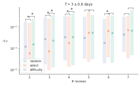
(a) T $=3\pm 0.8$ days

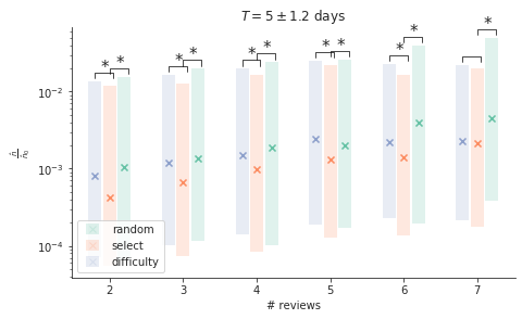
(b) T $=5\pm 1.2$ days

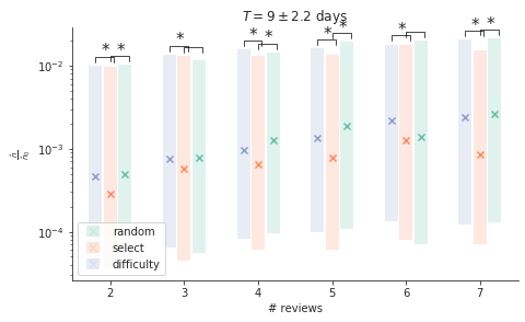
(c) T $=9\pm 2.2$ days

Figure 1: Normalized empirical forgetting rate (lower is better). Each triplet of bars in the figures corresponds to (learner, question) pairs in which the learner reviewed the question the same number of times (# reviews) for approximately the same period of time (T). Boxes indicate 25% and 75% quantiles and crosses indicate median values, where lower values indicate better performance. For each triple of bars, $*$ indicates a statistically significant difference (Matt-Whitney U-test; P-value = 0.05).

The results show that, in 83.5% of the cases, the empirical forgetting rate for the learners in the ‘select’ group is lower than that of the learners in the ‘difficulty’ and ‘random’ groups and, in 75% of cases, the decrease is statistically significant. Moreover, the median empirical forgetting rate for learners in the ‘select’ group is 48% lower than that of learners in the ‘random’ group and 40% lower than that of learners in the ‘difficulty’ group. In other words, the Select algorithm will help a median learner retain the answer to a median question 92% and 67% longer, respectively.

Next, we evaluate to what extent our algorithm can help increase (learner) engagement. To this end, we compare learners of the ‘select’, ‘difficulty’ and ‘random’ groups using Firebase Analytics. Table 1 summarizes the results, where engagement (retention in Firebase Analytics) indicates how likely is that a learner returns to the app within 4–7 days. We can conclude that, in terms of engagement, learners of the ‘select’ (‘difficulty’) group were 50.6% (47.6%) more likely, in median, to return to the app within 4–7 days than learners of the ‘random’ group. Moreover, Firebase Analytics estimates that, with probability 80%, the Select algorithm is the top performer in terms of engagement.

Algorithm	Median improvement in engagement (95%-ile)	Probability to be best
random	Baseline	$<0.1\%$
difficulty	+46.7% (+40.9% to +54.7%)	20%
select	+50.6% (+43.7% to +57.7%)	80%

Table 1: Learner engagement for the ‘random’, ‘difficulty’ and ‘select’ groups. Engagement indicates how likely is that a learner returns to the app within 4–7 days. The 95%-ile indicates the range in which the real value of the increase in engagement over baseline is contained with 95% probability.

Acknowledgements. We thank Robert West, Klein Lars Henning, Roland Aydin, and Behzad Tabibian for helpful conversations.

Appendix A Finding the optimal selection probabilities

In this section, we derive the optimal selection probabilities $\mathbf{p}(t)$ for the power-law memory model [16, 17] following a similar proof technique as in Tabibian et al. [12]. The derivation for the exponential memory model [14, 15] can be done similarly.

First, we express the dynamics of the forgetting rates $n_{i}(t)$ using the following stochastic differential equation (SDE) with jumps:

$$dn_{i}(t)=-\alpha_{i}n_{i}(t)r_{i}(t)dN_{i}(t)+\beta n_{i}(t)(1-r_{i}(t))dN_{i}(t)$$ (4)

where $E[dN_{i}(t)]=p_{i}(t)u(t)\,dt$. Now, we can use the above expression, Eq. 1 in the main paper, and Itö’s calculus [26] to express the dynamics of the recall probabilities $m_{i}(t)$ and the times since the last reviews $\Delta_{i}(t)$ using also SDEs with jumps, i.e.,

$$dm_{i}(t) =-\frac{n_{i}(t)m_{i}(t)dt}{(1+\Delta_{i}(t))}+(1-m_{i}(t))dN_{i}(t)$$ (5)

$$d\Delta_{i}(t) =dt-\Delta_{i}(t)dN_{i}(t)$$ (6)

Then, given the above expressions, we can decompose the optimization problem defined by Eq. 2 in the main paper into $K$ independent problems, i.e.,

$$\underset{p_{i}(t_{0},t_{f}]}{\text{minimize}}\leavevmode\nobreak\ \leavevmode\nobreak\ \mathbb{E}_{(N_{i},r_{i})(t_{0},t_{f}]}\big{[}\phi(m_{i}(t_{f}),n_{i}(t_{f}),\Delta_{i}(t_{f}))+\int_{t_{0}}^{t_{f}}\ell(m_{i}(\tau),n_{i}(\tau),\Delta_{i}(\tau),p_{i}(\tau))\,d\tau\big{]},$$ (7)

which can be solved separately.

Given a fixed question $i$, we denote $m(t)=m_{i}(t)$, $n(t)=n_{i}(t)$, $\Delta(t)=\Delta_{i}(t)$ and $p(t)=p_{i}(t)$, define the optimal cost-to-go function $J(m(t),n(t),\Delta(t),t)$ for the corresponding optimization problem as

$$J(m(t),n(t),\Delta(t),t)=\underset{p(t,t+dt]}{\text{min}}\mathbb{E}[J(m(t+dt),n(t+dt),\tau(t+dt),t+dt)]+\ell(m(t),n(t),\Delta(t),p(t))dt$$ (8)

and use Bellman’s principle of optimality to derive the corresponding HJB equation [26]. In particular, we can first rewrite the above equation as

$$0=\underset{p(t,t+dt]}{\text{min}}\mathbb{E}[dJ(m(t),n(t),\Delta(t),t)]+\ell(m(t),n(t),\Delta(t),p(t))dt,$$ (9)

where $dJ(m(t),n(t),\Delta(t),t)=J(m(t+dt),n(t+dt),\Delta(t+dt),t+dt)-J(m(t),n(t),\Delta(t),t)$, and then use the following technical Lemma, which can be proved using Itö’s calculus [26], to differentiate $J$ with respect to their parameters.

Lemma 1.

Let $x(t)$, $y(t)$, $k(t)$ be three jump-diffusion processes defined by the following jump SDEs:

$$dx(t)= f(x(t),y(t),k(t),t)dt+g(x(t),y(t),k(t),t)z(t)dN(t)+h(x(t),y(t),k(t),t)(1-z(t))dN(t)$$

$$dy(t)= p(x(t),y(t),k(t),t)dt+q(x(t),y(t),k(t),t)dN(t)$$

$$dk(t)= s(x(t),y(t),k(t),t)dt+v(x(t),y(t),k(t),t)dN(t)$$

where $N(t)$ is a jump process and $z(t)\in\{0,1\}$. If function $F(x(t),y(t),k(t),t)$ is once continuously differentiable in $x(t)$, $y(t)$, $k(t)$, and $t$, then,

$$dF(x(t),y(t),k(t),t) =(F_{t}+fF_{x}+pF_{y}+sF_{k})(x(t),y(t),k(t),t)dt$$

$$+\left[F(x+g,y+q,k+v,t)z(t)+F(x+h,y+q,k+v,t)(1-z(t))-F(x,y,t)\right]dN(t),$$

where for notational simplicity we dropped the arguments of the functions $f$, $g$, $h$, $p$ and $q$.

More specifically, we can write $dJ(m(t),n(t),\Delta(t),t)$ in Eq. 9 as

$$dJ(m(t),n(t),\Delta(t),t) =J_{t}(m(t),n(t),\Delta(t),t)-\frac{n(t)m(t)}{\Delta(t)+1}J_{m}(m(t),n(t),\Delta(t),t)+J_{\tau}(m,n,\tau,t)$$

$$+[J(1,(1-\alpha)n(t),0,t)r(t)+J(1,(1+\beta)n(t),0,t)(1-r(t))-$$

$$\leavevmode\nobreak\ \leavevmode\nobreak\ \leavevmode\nobreak\ \leavevmode\nobreak\ J(m(t),n(t),\Delta(t),t)]dN(t).$$

and thus write the HJB equation as:

$$0 =J_{t}(m(t),n(t),\Delta(t),t)-\frac{n(t)m(t)}{\Delta(t)+1}J_{m}(m(t),n(t),\Delta(t),t)+J_{\tau}(m(t),n(t),\Delta(t),t)$$

$$+\underset{u(t,t+dt]}{\text{min}}\big{\{}\ell(m(t),n(t),u(t))$$

$$+\left[J(1,(1-\alpha)n(t),0,t)m(t)+J(1,(1+\beta)n(t),0,t)(1-m(t))-J(m(t),n(t),\Delta(t),t)\right]p(t)u(t)\big{\}}$$ (10)

To solve the above differential equation, we need to define the loss $\ell$. Following the literature on stochastic control [26], we consider the following quadratic form, which penalizes quadratically the probability of unsuccessful recall of the answer to the question upon review and the probability of reviewing the question:

$$\ell(m(t),n(t),\Delta(t),p(t))=\frac{1}{2}(1-m(t))^{2}u(t)+\frac{1}{2}q\,p^{2}(t)u(t)$$ (11)

Now, if we plug in the above loss into the HJB equation and set its derivative with respect to $p(t)$ to zero to derive the optimal $p^{*}(t)$, we obtain:

$$p^{*}(t) =\frac{1}{q}\left[J(m(t),n(t),\Delta(t),t)-J(1,(1-\alpha)n(t),0,t)m(t)-J(1,(1+\beta)n(t),0,t)(1-m(t))\right]_{(0,q)},$$ (12)

where the operator $[\cdot]_{(a,b)}:=\min{(\max{(a,\cdot)},b)}$ is required to ensure that $0\leq p(t)\leq 1$. However, we will simplify these constraints to only positivity constraint and later verify that, by appropriately setting the tuning parameter $q$, we can make $p^{*}(t)\leq 1$ as well. Hence, if we plug in

$$p^{*}(t)=\frac{1}{q}\left[J(m(t),n(t),\Delta(t),t)-J(1,(1-\alpha)n(t),0,t)m(t)-J(1,(1+\beta)n(t),0,t)(1-m(t))\right]_{+}.$$ (13)

back into the HJB equation, we find that the optimal cost-to-go J needs to satisfy the following nonlinear differential equation:

$$0 =J_{t}(m(t),n(t),\Delta(t),t)-\frac{n(t)m(t)}{\Delta(t)+1}J_{m}(m(t),n(t),t)+J_{\tau}(m(t),n(t),\Delta(t),t)+\frac{1}{2}(1-m(t))^{2}$$

$$-\frac{u(t)}{2q}\left[J(m(t),n(t),\Delta(t),t)-J(1,(1-\alpha)n(t),0,t)m(t)-J(1,(1+\beta)n(t),0,t)(1-m(t))\right]_{+}^{2}.$$

To solve it, we rely on the following technical Lemma:

Lemma 2.

Consider the following family of losses with parameter $d>0$,

$$\ell_{d}(m(t),n(t),p(t)) =h_{d}(m(t),n(t),\Delta(t))+g_{d}^{2}(m(t),n(t))+\frac{1}{2}q\,p^{2}(t)u(t),$$

$$g_{d}(m(t),n(t)) =\sqrt{\frac{u(t)}{2}}\left[c_{2}\frac{\log(d)}{-m(t)^{2}+2m(t)-d}-c_{2}\frac{\log(d)}{1-d}+c_{1}m(t)\log\left(\frac{1+\beta}{1-\alpha}\right)-c_{1}\log(1+\beta)\right],$$

$$h_{d}(m(t),n(t),\Delta(t)) =-{\sqrt{q}}\frac{m(t)n(t)}{1+\Delta(t)}c_{2}\frac{(-2m(t)+2)\log(d)}{(-m(t)^{2}+2m(t)-d)^{2}}$$ (14)

where $c_{1},c_{2}\in\mathbb{R}$ are arbitrary constants. Then, the cost-to-go $J_{d}(m(t),n(t),\Delta(t),t)$ that satisfies the HJB equation, defined by Eq. 10, is given by:

$$J_{d}(m(t),n(t),\Delta(t),t) ={\sqrt{q}}\left(c_{1}\log(n(t))+c_{2}\frac{\log(d)}{-m(t)^{2}+2m(t)-d}\right)$$ (15)

$$\implies\frac{\partial J_{d}(m(t),n(t),\Delta(t),t)}{\partial t} =0$$ (16)

$$\frac{\partial J_{d}(m(t),n(t),\Delta(t),t)}{\partial\Delta} =0$$ (17)

$$\frac{\partial J_{d}(m(t),n(t),\Delta(t),t)}{\partial m(t)} =-c_{2}\frac{(-2m(t)+2)\log(d)}{(-m(t)^{2}+2m(t)-d)^{2}}$$ (18)

and the optimal intensity is given by:

$$p^{*}(t)=q^{-1/2}\left[c_{2}\frac{\log(d)}{-m(t)^{2}+2m(t)-d}-c_{2}\frac{\log(d)}{1-d}+c_{1}m(t)\log\left(\frac{1+\beta}{1-\alpha}\right)-c_{1}\log(1+\beta)\right]_{+}.$$

Proof.

Consider the family of losses defined by Eq. 14 and the functional form for the cost-to-go defined by Eq. 15. Then, for any parameter value $d>0$, the optimal intensity $p^{*}_{d}(t)$ is given by

$$p_{d}^{*}(t) =\frac{1}{q}\left[J_{d}(m(t),n(t),\Delta(t),t)-J_{d}(1,(1-\alpha)n(t),0,t)m(t)-J_{d}(1,(1+\beta)n(t),0,t)(1-m(t))\right]_{+}$$

$$=\frac{1}{\sqrt{q}}\left[c_{2}\frac{\log(d)}{-m^{2}+2m-d}-c_{2}\frac{\log(d)}{1-d}+c_{1}m(t)\log\left(\frac{1+\beta}{1-\alpha}\right)-c_{1}\log(1+\beta)\right]_{+},$$

and the HJB equation is satisfied:

$$\frac{\partial J_{d}(m,n,\Delta,t)}{\partial t}-\frac{mn}{1+\Delta}\frac{\partial J_{d}(m,n,\Delta,t)}{\partial m}+\frac{\partial J_{d}(m,n,\Delta,t)}{\partial\Delta}+h_{d}(m,n,\Delta)+g_{d}^{2}(m,n)$$

$$-\frac{u}{2q}\left[J_{d}(m,n,\Delta,t)-J_{d}(1,(1-\alpha)n,0,t)m-J_{d}(1,(1+\beta)n,0,t)(1-m)\right]_{+}^{2}$$

$$=\frac{mn}{1+\Delta}\underbrace{\sqrt{q}c_{2}\frac{(-2m+2)\log(d)}{(-m^{2}+2m-d)^{2}}}_{\frac{\partial J_{d}(m,n,\Delta,t)}{\partial m}}+h_{d}(m,n,\Delta)+g_{d}^{2}(m,n)$$

$$\quad-\frac{u}{2}\left[c_{1}\log(n)+c_{2}\frac{\log(d)}{-m^{2}+2m-d}-m\left(c_{1}\log(n(1-\alpha))+c_{2}\frac{\log(d)}{1-d}\right)-(1-m)\left(c_{1}\log(n(1+\beta))+c_{2}\frac{\log(d)}{1-d}\right)\right]_{+}^{2}$$

$$=\frac{mn}{1+\Delta}\sqrt{q}c_{2}\frac{(-2m+2)\log(d)}{(-m^{2}+2m-d)^{2}}\underbrace{-\sqrt{q}\frac{mn}{1+\Delta}c_{2}\frac{(-2m+2)\log(d)}{(-m^{2}+2m-d)^{2}}}_{h_{d}(m,n,\Delta)}$$

$$\quad-\frac{u}{2}\big{[}c_{2}\frac{\log(d)}{-m^{2}+2m-d}-c_{2}\frac{\log(d)}{1-d}+c_{1}m\log(\frac{1+\beta}{1-\alpha})-c_{1}\log(1+\beta)\big{]}_{+}^{2}$$

$$\quad+\underbrace{\frac{u}{2}\big{[}c_{2}\frac{\log(d)}{-m^{2}+2m-d}-c_{2}\frac{\log(d)}{1-d}+c_{1}m\log(\frac{1+\beta}{1-\alpha})-c_{1}\log(1+\beta)\big{]}_{+}^{2}}_{g_{d}(m,n)^{2}}=0,$$

where for notational simplicity $m=m(t)$, $n=n(t)$, $\Delta=\Delta(t)$ and $u=u(t)$. ∎

More specifically, note that $\lim_{d\rightarrow 1}l_{d}(m(t),n(t),p(t))=\frac{1}{2}(1-m(t))^{2}u(t)+\frac{1}{2}q\,p^{2}(t)u(t)$ and thus

$$p^{*}(t)=\lim_{d\rightarrow 1}p^{*}_{d}(t)=\frac{1}{\sqrt{q}}\left[c_{1}m(t)\log{\frac{1+\beta}{1-\alpha}}-c_{1}\log{(1+\beta)}-c_{2})\right]$$

Then, if we set $c_{1}=\frac{1}{\log{\frac{1-\alpha}{1+\beta}}}$ and $c_{2}=\frac{\log{(1-\alpha)}}{\log{\frac{1-\alpha}{1+\beta}}}$, we can readily conclude that the optimal selection probability is given by:

$$p^{*}(t)=\frac{1}{\sqrt{q}}(1-m(t))$$ (19)

Finally, note that $1-m(t)\in[0,1]$ and hence, as long as $q\geq 1$, we have $p^{*}(t)\leq 1$, which will satisfy the constraints required in Eq. 12.

Appendix B Additional details on iTheorie Führerschein Auto

Learners use the iTheorie Führerschein Auto to prepare for the written section of the driving lessons. When a learner installs the app, she is assigned to one of the three item selection algorithms randomly via Google Analytics. The learner does not know which item selection algorithm has been used to create his or her study sessions.

Upon starting the app, the learners are greeted with a screen where they can select the lessons they would like to take, shown in Figure 2a. Once they select a category, a study session starts and they are given questions to answer, as shown in Figure 2b. The selection of items in each section is done using the algorithm assigned to the user by Google Analytics. A study session continues until the learner takes a break of longer than 5 minutes. Figures 2c and 2d show the notification shown to the user after a correct and incorrect answer respectively.

(a) Lesson selection

(b) Session start

(c) Correct response

(d) Incorrect response

Figure 2: The iTheory learning app.

Appendix C Predictive performance of the memory model

In this section, we evaluate the predictive performance of the exponential and the power-law memory models using data from February 2019 to June 2019. In both cases, we fit the model parameters $n_{i}(0)$, $\alpha$ and $\beta$ using the variant of half-life regression proposed by Tabibian et al.. [See Appendix, Section 8] and performed a grid search to determine the optimal values of the hyper-parameters.

Table 2 summarizes the results. In terms of mean average error (MAE) in predicting the recall of items and in terms of correlation between the predicted and empirically observed half-life for the items (COR_h), the exponential model clearly outperforms the power-law model. However, in terms of Area Under the Curve (AUC), the power-law model performs slightly better than the exponential model.

Given these results, we decided to use the exponential memory model to estimate the recall probability during our randomized controlled trial.

	Exponential	Power-law
MAE$\downarrow$	0.139	0.282
AUC$\uparrow$	0.887	0.901
COR${}_{h}\uparrow$	0.611	0.571

Table 2: Predictive performance of the exponential and power-law forgetting curve models. The arrows indicate whether a higher value of the metric is better ($\uparrow$) or a lower value ($\downarrow$).

References

- [1] Michael C Mozer, Melody Wiseheart, and Timothy P Novikoff. Artificial intelligence to support human instruction. Proceedings of the National Academy of Sciences, 116(10):3953–3955, 2019.
- [2] Florian Sense, Tiffany S Jastrzembski, Michael C Mozer, Michael Krusmark, and Hedderik van Rijn. Perspectives on computational models of learning and forgetting. In International Conference on Cognitive Modeling, 2019.
- [3] Joel Brewster Lewis and Nan Li. Combinatorial aspects of flashcard games. Annals of Combinatorics, 18(3):459–472, 2014.
- [4] Joel Nishimura. Critically slow learning in flashcard learning models. Chaos: An Interdisciplinary Journal of Nonlinear Science, 28(8):083115, 2018.
- [5] Timothy P Novikoff, Jon M Kleinberg, and Steven H Strogatz. Education of a model student. Proceedings of the National Academy of Sciences, 109(6):1868–1873, 2012.
- [6] Siddharth Reddy, Igor Labutov, Siddhartha Banerjee, and Thorsten Joachims. Unbounded human learning: Optimal scheduling for spaced repetition. In Proceedings of the 22nd ACM SIGKDD international conference on knowledge discovery and data mining, pages 1815–1824, 2016.
- [7] Anette Hunziker, Yuxin Chen, Oisin Mac Aodha, Manuel Gomez Rodriguez, Andreas Krause, Pietro Perona, Yisong Yue, and Adish Singla. Teaching multiple concepts to a forgetful learner. In Advances in Neural Information Processing Systems, pages 4048–4058, 2019.
- [8] Philip I Pavlik and John R Anderson. Using a model to compute the optimal schedule of practice. Journal of Experimental Psychology: Applied, 14(2):101, 2008.
- [9] Claudia Metzler-Baddeley and Roland J Baddeley. Does adaptive training work? Applied Cognitive Psychology: The Official Journal of the Society for Applied Research in Memory and Cognition, 23(2):254–266, 2009.
- [10] Robert V Lindsey, Jeffery D Shroyer, Harold Pashler, and Michael C Mozer. Improving students’ long-term knowledge retention through personalized review. Psychological science, 25(3):639–647, 2014.
- [11] Burr Settles and Brendan Meeder. A trainable spaced repetition model for language learning. In Proceedings of the 54th annual meeting of the association for computational linguistics (volume 1: long papers), pages 1848–1858, 2016.
- [12] Behzad Tabibian, Utkarsh Upadhyay, Abir De, Ali Zarezade, Bernhard Schölkopf, and Manuel Gomez-Rodriguez. Enhancing human learning via spaced repetition optimization. Proceedings of the National Academy of Sciences, 116(10):3988–3993, 2019.
- [13] Henry L Roediger III and Jeffrey D Karpicke. Test-enhanced learning: Taking memory tests improves long-term retention. Psychological science, 17(3):249–255, 2006.
- [14] Odd Aalen, Ornulf Borgan, and Hakon Gjessing. Survival and event history analysis: a process point of view. Springer Science & Business Media, 2008.
- [15] John T Wixted, Shana K Carpenter, et al. The wickelgren power law and the ebbinghaus savings function. Psychological Science, 18(2):133, 2007.
- [16] Lee Averell and Andrew Heathcote. The form of the forgetting curve and the fate of memories. Journal of Mathematical Psychology, 55(1):25–35, 2011.
- [17] Hermann Ebbinghaus. Memory: A contribution to experimental psychology. 1885.
- [18] Geoffrey R Loftus. Evaluating forgetting curves. Journal of Experimental Psychology: Learning, Memory, and Cognition, 11(2):397, 1985.
- [19] Floyd B Hanson. Applied stochastic processes and control for jump-diffusions: modeling, analysis and computation. SIAM, 2007.