Baseline System of Voice Conversion Challenge 2020 with Cyclic Variational Autoencoder and Parallel WaveGAN

Abstract

In this paper, we present a description of the baseline system of Voice Conversion Challenge (VCC) 2020 with a cyclic variational autoencoder (CycleVAE) and Parallel WaveGAN (PWG), i.e., CycleVAEPWG. CycleVAE is a nonparallel VAE-based voice conversion that utilizes converted acoustic features to consider cyclically reconstructed spectra during optimization. On the other hand, PWG is a non-autoregressive neural vocoder that is based on a generative adversarial network for a high-quality and fast waveform generator. In practice, the CycleVAEPWG system can be straightforwardly developed with the VCC 2020 dataset using a unified model for both Task 1 (intralingual) and Task 2 (cross-lingual), where our open-source implementation is available at https://github.com/bigpon/vcc20_baseline_cyclevae. The results of VCC 2020 have demonstrated that the CycleVAEPWG baseline achieves the following: 1) a mean opinion score (MOS) of 2.87 in naturalness and a speaker similarity percentage (Sim) of 75.37% for Task 1, and 2) a MOS of 2.56 and a Sim of 56.46% for Task 2, showing an approximately or nearly average score for naturalness and an above average score for speaker similarity.

Index Terms: voice conversion challenge, CycleVAE, nonparallel spectral modeling, cross-lingual, Parallel WaveGAN

1 Introduction

Voice conversion (VC) [1] is a framework for changing the voice characteristics of a source speaker into those of a desired target speaker while retaining the linguistic contents of the source speech. VC is very useful for many real-world applications, such as speech database augmentation [2], improvement of impaired speech [3], entertainment purposes [4], expressive speech synthesis [5], and improvement of speaker verification systems [6]. To support the research and development of VC techniques, during the past six years, three VC challenges have been carried out, i.e., VC challenge (VCC) 2016 [7], VCC 2018 [8], and VCC 2020 [9]. In this paper, we provide a description for a baseline system in VCC 2020, where our goal is to provide a straightforward baseline implementation using freely available software that can be developed even with only the VCC 2020 dataset.

In performing VC, the changes in characteristics can be affected by mainly two factors, namely, voice timbre and prosody. Voice timbre is related to the spectral characteristics of the vocal tract during phonation, whereas prosody is related to suprasegmental factors, such as pitch/intonation, duration, and stress. To develop a clear-cut implementation, in this work, we keep the duration of the speech unchanged and use a transformation of fundamental frequency (F0) to change pitch characteristics. On the other hand, we focus on the VC development using a mapping model for spectral features, such as mel-cepstrum parameters [10] obtained from the vocal tract spectral envelope.

Spectral modeling in VC can be developed in two ways, i.e., the parallel method using paired utterances between speakers and the nonparallel method without using paired utterances. Many methods have been developed for parallel spectral modeling, such as the codebook-based method [1], methods using the Gaussian mixture model [11, 12], methods using dynamic kernel partial least squares regression [13], and the exemplar-based method [14]. The nonparallel spectral modeling approach has also been adopted in the recent years for the frequency warping method [15], restricted Boltzmann machine [16], generative adversarial network [17], and variational autoencoder (VAE)-based model [18], among others. In this paper, considering the versatility of the nonparallel method, especially for cross-lingual VC, we focus on the use of nonparallel VAE-based spectral modeling.

VAE-based VC is usually developed by assuming that the latent space contains speaker-independent characteristics, such as phonetics, while the speaker-dependent space is handled with a time-invariant one-hot speaker code [18]. However, as has been studied in [19], optimization with only spectral features reconstruction does not yield sufficient conversion performance. It has been found that with a cycle-consistent approach, i.e., cyclic VAE (CycleVAE), significant improvements have been observed for the accuracy of converted speech. During the optimization of a CycleVAE, converted spectral features that are generated with the speaker code of the desired target speaker are used to generate cyclically reconstructed spectra that can also be optimized.

To synthesize a converted speech waveform from converted acoustic features generated from a VC model, two different approaches can be used, i.e., using a conventional vocoder, such as STRAIGHT [20] or WORLD [21], and using a neural vocoder, such as WaveNet [22, 23]. The latter is capable of producing natural-quality speech in a copy-synthesis procedure and natural-to-high-quality speech in text-to-speech [24] or VC [25] systems. In this work, instead of using an autoregressive (AR) neural vocoder, such as WaveNet, we use a non-AR neural vocoder that generates waveform samples in parallel, which will be more convenient for user-friendly baseline implementation. In particular, we use the recent non-AR neural vocoder based on a generative adversarial network (GAN), i.e., Parallel WaveGAN (PWG) [26], which provides real-time decoding with GPU and is able to generate high-quality output.

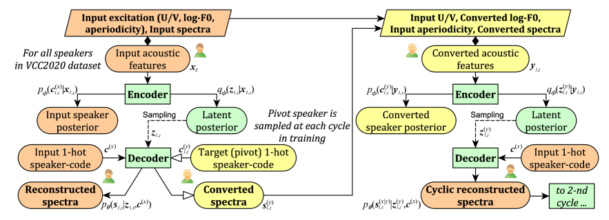
Figure 1: Process flow of CycleVAE-based spectral modeling within the 1${}^{\text{st}}$ cycle, where converted acoustic features of a sampled target (pivot) speaker are used to generate cyclically reconstructed spectra that can also be utilized during optimization. (pale-orange color refers to input-speaker part; pale-yellow color refers to pivot-/target-speaker part; green color refers to speaker-normalized part)

To obtain better converted speech waveforms, we further reduce the mismatches [27] between the typical natural acoustic features used to train a neural vocoder and the converted acoustic features generated from a VC model. Specifically, we obtain reconstructed and cyclically reconstructed spectra from a CycleVAE-based spectral model, and use them alongside the natural spectra to train a PWG-based neural vocoder. In practice, the CycleVAE and PWG (CycleVAEPWG) baseline system can be developed in a straightforward manner using our open-source implementation with the VCC 2020 dataset.

2 CycleVAE-based Spectral Modeling

2.1 Model formulation

Let $\bm{{x}}_{t}=[\bm{{s}}^{(x)^{\top}}_{t},\bm{{e}}^{(x)^{\top}}_{t}]^{\top}$ be an input acoustic feature vector, where $\bm{{s}}^{(x)}_{t}$ and $\bm{{e}}^{(x)}_{t}$ respectively denote an input spectral feature vector, such as that of mel-cepstrum parameters, and an input excitation feature vector, such as that of fundamental frequency (F0), unvoiced/voiced (U/V) decision, and aperiodicity, at time $t$. Likewise, the target (pivot) acoustic feature vector is denoted as $\bm{{y}}_{t}=[\bm{{s}}^{(y)^{\top}}_{t},\bm{{e}}^{(y)^{\top}}_{t}]^{\top}$ and the input acoustic feature vector conditioned on the pivot speaker is denoted as $\bm{{x}}^{(y)}_{t}=[\bm{{s}}^{(x|y)^{\top}}_{t},\bm{{e}}^{(x|y)^{\top}}_{t}]^{\top}$ at time $t$.

As described in [19, 28], the variational lower bound for the CycleVAE model at the $n$-th cycle is given by

$$\mathcal{L}(\bm{{\theta}}\!,\bm{{\phi}};\bm{{x}}_{n,t},\bm{{x}}_{n,t}^{(y)})\!=\!\mathbb{E}_{q_{\bm{{\phi}}}(\bm{{z}}_{n,t}|\bm{{x}}_{n,t})}[\log p_{\bm{{\theta}}}(\bm{{s}}^{(x)}_{n,t}\!=\!\bm{{s}}^{(x)}_{t}|\bm{{z}}_{n,t},\bm{{c}}^{(x)})]$$

$$\>+\mathbb{E}_{q_{\bm{{\phi}}}(\bm{{z}}^{(y)}_{n,t}|\bm{{y}}_{n,t})}[\log p_{\bm{{\theta}}}(\bm{{s}}^{(x|y)}_{n,t}=\bm{{s}}^{(x)}_{t}|\bm{{z}}^{(y)}_{n,t},\bm{{c}}^{(x)})]$$

$$\>-\!D_{\text{KL}}(q_{\bm{{\phi}}}(\bm{{z}}_{n,t}|\bm{{x}}_{n,t})||p_{\bm{{\theta}}}(\bm{{z}}_{n,t}))\!-\!D_{\text{KL}}(q_{\bm{{\phi}}}(\bm{{z}}^{(y)}_{n,t}|\bm{{y}}_{n,t})||p_{\bm{{\theta}}}(\bm{{z}}^{(y)}_{n,t}))$$

$$\>+\log p_{\bm{{\phi}}}(\bm{{c}}^{(x)}_{n,t}\!=\!\bm{{c}}^{(x)}|\bm{{x}}_{n,t})\!+\!\log p_{\bm{{\phi}}}(\bm{{c}}^{(y)}_{n,t}\!=\!\bm{{c}}^{(y)}_{n}|\bm{{y}}_{n,t}),\!\!\!\!$$ (1)

where

$$\bm{{s}}^{(x)}_{n,t} =g_{\bm{{\theta}}}(\bm{{z}}_{n,t},\bm{{c}}^{(x)});\bm{{s}}^{(x|y)}_{n,t}=g_{\bm{{\theta}}}(\bm{{z}}^{(y)}_{n,t},\bm{{c}}^{(x)}),$$ (2)

$$\bm{{z}}_{n,t} =f_{\bm{{\phi}}}(\bm{{x}}_{n,t})^{(\bm{{\mu}})}-f_{\bm{{\phi}}}(\bm{{x}}_{n,t})^{(\bm{{\sigma}})}\odot\bm{{\epsilon}},$$ (3)

$$\bm{{z}}^{(y)}_{n,t} =f_{\bm{{\phi}}}(\bm{{y}}_{n,t})^{(\bm{{\mu}})}-f_{\bm{{\phi}}}(\bm{{y}}_{n,t})^{(\bm{{\sigma}})}\odot\bm{{\epsilon}},$$ (4)

$$\bm{{\epsilon}} =\operatorname{sign}(\bm{{U}})\ln(1\!-\!2|\bm{{U}}|),\,\text{s.t.}\>\bm{{U}}\!\!\sim\!(-1/2,1/2],$$ (5)

$$\bm{{x}}_{n,t} =[\bm{{s}}^{(x|y)^{\top}}_{n-1,t},\bm{{e}}^{(x)^{\top}}_{t}]^{\top};\bm{{s}}^{(x|y)}_{0,t}=\bm{{s}}^{(x)}_{t}$$ (6)

$$\bm{{y}}_{n,t} =[\bm{{s}}^{(y)^{\top}}_{n,t},\bm{{e}}^{(y)^{\top}}_{n,t}]^{\top};\bm{{s}}^{(y)}_{n,t}=g_{\bm{{\theta}}}(\bm{{z}}_{n,t},\bm{{c}}^{(y)}_{n}),$$ (7)

$$\bm{{c}}^{(x)}_{n,t} =f_{\bm{{\phi}}}(\bm{{x}}_{n,t})^{(\bm{{c}})};\bm{{c}}^{(y)}_{n,t}=f_{\bm{{\phi}}}(\bm{{y}}_{n,t})^{(\bm{{c}})},$$ (8)

$$p_{\bm{{\theta}}}(\bm{{z}}_{n,t}) =p_{\bm{{\theta}}}(\bm{{z}}^{(y)}_{n,t})=\mathcal{L}(\bm{{0}},\bm{{I}});\bm{{c}}^{(y)}_{n}\in\bm{{C}}\setminus\bm{{c}}^{(x)}.$$ (9)

Here, the time-invariant speaker code of the input speaker is denoted as $\bm{{c}}^{(x)}$ and that of the pivot speaker is denoted as $\bm{{c}}^{(y)}_{n}$. The set of all available speaker codes is denoted as $\bm{{C}}$.

The set of parameters of the inference (encoder) network and that of the generative (decoder) network are respectively denoted as $\bm{{\phi}}$ and $\bm{{\theta}}$. The feedforward functions of the encoder and decoder are respectively denoted as $f_{\bm{{\phi}}}(\cdot)$ and $g_{\bm{{\theta}}}(\cdot)$. The latent feature vectors are denoted as $\bm{{z}}_{n,t}$ and $\bm{{z}}_{n,t}^{(y)}$. The standard Laplacian distribution is denoted as $\mathcal{L}(\bm{{0}},\bm{{I}})$. The encoder network outputs the parameters of latent posterior distribution, i.e., location ($\bm{{\mu}}$) and scale ($\bm{{\sigma}}$), and the logits of speaker posterior ($\bm{{c}}$). The excitation feature vector of the sampled target speaker at the $n$-th cycle $\bm{{e}}^{(y)}_{n,t}$ consists of the transformed F0 [12], input U/V decisions, and the input aperiodicity of $\bm{{e}}^{(x)}_{t}$.

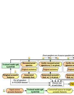
Figure 2: Process flow for data augmentation with generated acoustic features from CycleVAE-based spectral model to train PWG-based neural vocoder, which is used to generate converted speech from the converted acoustic features in the conversion phase. (pale-orange color refers to source-speaker features part; pale-yellow color refers to target-speaker features part; gradient pale-orange-yellow color refers to the features set of all speakers; gradient orange-yellow color refers to the waveform set of all speakers)

2.2 Network architecture and training procedure

An overview of the process flow for the CycleVAE-based spectral model, as described in Eqs. (1)–(9), is shown in Fig. 1. The CycleVAE network architecture [19] consists of convolutional input layers and a recurrent layer with one fully connected output layer, where its output is fed back to the recurrent layer. This structure applies to both encoder and decoder networks. The extraction of acoustic features requires the annotation of the F0 range and power threshold values for each speaker, as described in [29]. During optimization, a power threshold is used to automatically discard starting and ending silence frames. A loss function based on mel-cepstral distortion [12] is used for the conditional probability density function (pdf) terms of the spectral features in Eq. (1), whereas a cross-entropy loss function is used for the corresponding conditional pdf terms of the speaker codes. In this baseline system, only the VCC 2020 dataset is used to develop the CycleVAE-based spectral model, as well as the PWG-based neural vocoder.

3 PWG-based Neural Vocoder

3.1 Network architecture and optimization

Parallel WaveGAN (PWG) [26] is a GAN-based neural vocoder composed of a generator (G) network and a discriminator (D) network. The generator network is designed to be similar to the WaveNet architecture conditioned on auxiliary acoustic features, where the output layer directly generates waveform samples in parallel from input noise. The generator learns the waveform distribution by trying to deceive the discriminator in identifying the generated waveform samples as the real ones, i.e., adversarial training. The discriminator tries to identify the original waveform samples as the real ones and the generated waveform samples as the fake ones. To improve the modeling of waveform samples, a set of multiresolution short-time Fourier transform (STFT) losses is also further included.

3.2 Training procedure with data augmentation

In this system, we perform data augmentation for the acoustic features to obtain a more robust PWG-based neural vocoder with respect to the mismatches [27] between naturally extracted spectral features $\bm{{s}}^{(x)}_{t}$ and converted spectral features $\bm{{s}}^{(y)}_{1,t}$, which are generated from the CycleVAE model as given in Section 2.1. Specifically, reconstructured spectral features $\bm{{s}}^{(x)}_{1,t}$ and cyclically reconstructed spectral features $\bm{{s}}^{(x|y)}_{1,t}$ are used alongside the natural spectral features $\bm{{s}}^{(x)}_{t}$ to train the PWG, as shown in Fig. 2.

Therefore, the optimization for PWG can be written as

$$\{\hat{\bm{{\vartheta}}},\hat{\bm{{\varphi}}}\}=\operatorname*{arg\,min}_{\bm{{\vartheta}}}\operatorname*{arg\,max}_{\bm{{\varphi}}}\mathbb{E}_{\bm{{h}}}[(1-D_{\bm{{\varphi}}}(G_{\bm{{\vartheta}}}(\bm{{h}}|\bm{{x}})))^{2}]$$

$$+\!\!\mathbb{E}_{\bm{{h}}}[(1\!-\!D_{\bm{{\varphi}}}(G_{\bm{{\vartheta}}}(\bm{{h}}|\hat{\bm{{x}}})))^{2}]\!+\!\sum_{p=1}^{P}\!\mathbb{E}_{\bm{{h}}}[(1\!-\!D_{\bm{{\varphi}}}(G_{\bm{{\vartheta}}}(\bm{{n}}|\hat{\bm{{x}}}^{(y_{p})})))^{2}]$$

$$+\!\!\mathbb{E}_{\bm{{w}}}[D_{\bm{{\varphi}}}(\bm{{w}})^{2}]\!+\!\mathbb{E}_{\bm{{h}},\bm{{w}}}[\text{STFT}_{\!m}\!(\bm{{w}},\!\hat{\bm{{w}}})]\!+\!\mathbb{E}_{\bm{{h}}\!,\bm{{w}}}[\text{STFT}_{\!m}\!(\bm{{w}}\!,\!\hat{\bm{{w}}}^{(x)})]$$

$$+\!\!\sum_{p=1}^{P}\!\mathbb{E}_{\bm{{h}}\!,\bm{{w}}\!}[\text{STFT}_{\!m}\!(\bm{{w}}\!,\!\hat{\bm{{w}}}^{(x|y_{p})})]\,\text{s.t}\,\bm{{h}}\!\sim\!\!\mathcal{N}(0,\!I),\!\bm{{w}}\!\!\sim\!\!p(\bm{{w}}),\!\!\!$$ (10)

where $\bm{{h}}=[h_{1},\dotsc,h_{T}]^{\top}$ denotes the sequence of white noise and the standard Gaussian distribution is denoted as $\mathcal{N}(0,I)$. The parameter sets of the generator and discriminator are denoted as $\bm{{\vartheta}}$ and $\bm{{\varphi}}$, respectively. The sequences of real and generated waveform samples are denoted as $\bm{{w}}=[w_{1},\dotsc,w_{T}]^{\top}$ and $\hat{\bm{{w}}}=[\hat{w}_{1},\dotsc,\hat{w}_{T}]^{\top}$, respectively, where $\hat{\bm{{w}}}=G_{\bm{{\vartheta}}}(\bm{{h}}|\bm{{x}})$. The distribution of the real waveform samples is denoted as $p(\bm{{w}})$. $\text{STFT}_{\!m}(\cdot)$ denotes $m$ sets of multiresolution STFT losses as in [26]. $\hat{\bm{{x}}}=[\hat{\bm{{x}}}_{1}^{\top},\dotsc,\hat{\bm{{x}}}_{T}^{\top}]^{\top}$ denotes the sequence of reconstructed acoustic features with $\hat{\bm{{x}}}_{t}=[\bm{{s}}_{1,t}^{(x)},\bm{{e}}^{(x)}_{t}]^{\top}$ and $\hat{\bm{{x}}}^{(y_{p})}=[\hat{\bm{{x}}}^{(y_{p})^{\top}}_{1},\dotsc,\hat{\bm{{x}}}^{(y_{p})^{\top}}_{T}]^{\top}$ denotes the sequence of cyclically reconstructed acoustic features with $\hat{\bm{{x}}}^{(y_{p})}_{t}=[\bm{{s}}_{1,t}^{(x|y_{p})},\bm{{e}}^{(x)}_{t}]^{\top}$. Hence, $\hat{\bm{{w}}}^{(x)}=G_{\bm{{\vartheta}}}(\bm{{h}}|\hat{\bm{{x}}}^{(x)})$ and $\hat{\bm{{w}}}^{(x|y_{p})}=G_{\bm{{\vartheta}}}(\bm{{h}}|\hat{\bm{{x}}}^{(x|y_{p})})$. For each speaker $x$, the number of pivot speakers $p$ to generate cyclically reconstructed spectra $\bm{{s}}_{1,t}^{(x|y_{p}))}$ in Eq. (2) is $P$.

4 Results of VCC 2020

4.1 CycleVAEPWG baseline system conditions

We used WORLD [21] to perform acoustic feature extraction. As the spectral features, $49$-dimensional mel-cepstrum parameters, including the $0$-th power coefficient, were extracted from the speech spectral envelope with $0.466$ frequency warping coefficient. CheapTrick [30] was used to extract the spectral envelope, Harvest [31] was used to extract F0 values, and D4C [32] was used to extract the aperiodicity spectrum, which was interpolated into $3$-dimensional code aperiodicity. The sampling rate of the speech signal was $24000~{}$Hz. The number of FFT points in the analysis was $2048$. The frame shift was set to $5~{}$ms.

The VCC 2020 dataset [9] consisted of 14 speakers, where 4 of them were the source speakers and the remaining 10 were the target speakers. The set of source speakers consisted of 2 male and 2 female English speakers. The set of target speakers consisted of another 4 English speakers (2 males and 2 females), 2 German, 2 Finnish, and 2 Mandarin speakers, where the latter three sets consisted of 1 male and 1 female. The number of utterances for each speaker was 70 in the speaker’s language. The English sets had 20 parallel utterances between the source and target speakers. The sets of each of the other languages were parallel. To train both CycleVAE and PWG, 60 utterances from each speaker were used in the training set, whereas the remaining 10 utterances were used in the validation set. The evaluation set in the official test consisted of another 25 utterances in English. Task 1 of VCC 2020 was intralingual conversion, whereas Task 2 was cross-lingual conversion. The CycleVAEPWG baseline system was developed using only the VCC 2020 dataset.

Figure 3: Evaluation result of VCC 2020 Task 1 (intralingual conversion) consisting of MOS for naturalness ($x$-axis) and speaker-similarity percentage ($y$-axis), where the CycleVAEPWG baseline is denoted as T16, the other baseline systems are denoted as T11 and T22, and the top system is denoted as T10. The values are the average of the results of Japanese and English listeners. The average of all systems (31 including 3 baseline systems) is denoted as Avg.

Our CycleVAEPWG implementation is freely available at https://github.com/bigpon/vcc20_baseline_cyclevae. The hyperparameters of CycleVAE were those in [19]. The differences were that the CycleVAE of VCC 2020 baseline system was implemented for many-to-many VC on a unified encoder–decoder using standard Laplacian prior and only 2 cycles as in [28]. The CycleVAE spectral model was trained for $\sim\!\!2$ days with NVIDIA Titan V.

The hyperparameters of PWG were those in [26] with the same configurations for STFT losses. The difference was that the conditioning acoustic features consisted of mel-cepstrum parameters and the same excitation parameters as in [33]. Furthermore, the generator of PWG was trained for 100K steps without a discriminator and adversarial losses, i.e., only STFT losses, and another 300K steps with a discriminator and adversarial losses. For the data augmentation procedure described in Section 3.2, each of the 4 source speakers had the 10 target speakers as the pivot speakers $p$, and vice versa. The PWG neural vocoder was trained for $\sim\!\!3$ days with NVIDIA Titan V.

4.2 VCC 2020 evaluation conditions

In the VCC 2020 evaluation [9], a large-scale listening test was conducted, where there were 206 Japanese listeners and 68 English listeners. There were three baseline systems including CycleVAEPWG for both Tasks 1 and 2. The total number of participant systems including the three baseline systems for Task 1 was 31, whereas that for Task 2 was 28. The listening test consisted of 1) naturalness evaluation, where each listener was asked to evaluate the naturalness of each audio sample using a 5-scale mean opinion score (MOS), and 2) speaker similarity evaluation, where each listener was presented with two audio samples (converted and reference) and asked to evaluate whether the two samples were produced by the same speaker using a 4-scale similarity score. In the evaluation results, the baseline CycleVAEPWG is denoted as T16, whereas the other two baseline systems are denoted as T11 [25] and T22 [34]. The top system in the VCC 2020 is denoted as T10.

Figure 4: Evaluation result of VCC 2020 Task 2 (cross-lingual conversion) consisting of MOS for naturalness ($x$-axis) and speaker-similarity percentage ($y$-axis), where the CycleVAEPWG baseline is denoted as T16, the other baseline systems are denoted as T11 and T22, and the top system is denoted as T10. The values are the average of the results of Japanese and English listeners. The average of all systems (28 including 3 baseline systems) is denoted as Avg.

4.3 Evaluation results of Tasks 1 and 2

The result of Task 1 (intralingual) is shown in Fig. 3 and the result of Task 2 (cross-lingual) is shown in Fig. 4, where the average score of all participant systems including the baseline systems is denoted as Avg. The values are the average results of Japanese and English listeners. It can be observed that for Tasks 1 and 2, the CycleVAEPWG baseline achieves similarity percentages of 75.37% and 56.46%, which are above the average similarity percentages of 66.76% and 50.03%, respectively. As for naturalness, the CycleVAEPWG baseline achieves MOSs of 2.87 and 2.56 for Tasks 1 and 2, respectively, which are about the same as the average MOS for Task 1 and below the average MOS for Task 2, i.e., 2.89 and 2.81, respectively. Note that one other team, T23 [35], also uses the CycleVAE-based spectral model, but with the AR neural vocoder, i.e., WaveNet, for Task 2, which yields a significantly higher MOS of 3.20.

5 Conclusions

We have presented the description of CycleVAEPWG baseline system for the VCC 2020. The CycleVAEPWG baseline consists of the cyclic variational autoencoder (CycleVAE)-based spectral model and Parallel WaveGAN (PWG)-based neural vocoder, which is developed with only the VCC 2020 dataset using freely available software. In the training, CycleVAE optimizes reconstructed and cyclically reconstructed spectra, where the latter is obtained by recycling converted acoustic features. The results of VCC 2020 have demonstrated that the CycleVAEPWG baseline 1) achieves an average MOS of approximately 2.87 for naturalness for Task 1 (intralingual) and a below average MOS of 2.56 for Task 2 (cross-lingual), 2) achieves above average speaker similarity percentages of 75.37% and 56.46% for Tasks 1 and 2, respectively. This system merits further research because of its solid performance for intra- and cross-lingual VC, and its clear-cut implementation, which is freely available.

6 Acknowledgements

This work was partly supported by JSPS KAKENHI Grant Number 17H06101 and JST, CREST Grant Number JPMJCR19A3.

References

- [1] M. Abe, S. Nakamura, K. Shikano, and H. Kuwabara, “Voice conversion through vector quantization,” J. Acoust. Soc. of Jpn. (E), vol. 11, no. 2, pp. 71–76, 1990.
- [2] A. Kain and M. W. Macon, “Spectral voice conversion for text-to-speech synthesis,” in Proc. ICASSP, Seatle, Washington, USA, May 1998, pp. 285–288.
- [3] K. Tanaka, T. Toda, G. Neubig, S. Sakti, and S. Nakamura, “A hybrid approach to electrolaryngeal speech enhancement based on spectral subtraction and statistical voice conversion,” in Proc. INTERSPEECH, Lyon, France, Sep. 2013, pp. 3067–3071.
- [4] K. Kobayashi, T. Toda, and S. Nakamura, “Intra-gender statistical singing voice conversion with direct waveform modification using log-spectral differential,” Speech Commun., vol. 99, pp. 211–220, 2018.
- [5] O. Türk and M. Schröder, “Evaluation of expressive speech synthesis with voice conversion and copy resynthesis techniques,” IEEE/ACM Trans. Audio Speech Lang. Process., vol. 18, no. 5, pp. 965–973, 2010.
- [6] M. Todisco, X. Wang, V. Vestman, M. Sahidullah, H. Delgado, A. Nautsch, J. Yamagishi, N. Evans, T. Kinnunen, and K. A. Lee, “ASVspoof 2019: Future horizons in spoofed and fake audio detection,” in Proc. INTERSPEECH, Graz, Austria, Sep. 2019, pp. 1008–1012.
- [7] T. Toda, L.-H. Chen, F. Villavicencio, Z. Wu, and J. Yamagishi, “The Voice Conversion Challenge 2016,” in Proc. INTERSPEECH, San Francisco, USA, Sep. 2016, pp. 1632–1636.
- [8] J. Lorenzo-Trueba, J. Yamagishi, T. Toda, D. Saito, F. Villavicencio, T. Kinnunen, and Z. Ling, “The Voice Conversion Challenge 2018: Promoting development of parallel and nonparallel methods,” in Proc. Odyssey, Les Sables d’Olonne, France, Jun. 2018, pp. 195–202.
- [9] Y. Zhao, W.-C. Huang, X. Tian, J. Yamagishi, R. K. Das, T. Kinnunen, Z. Ling, and T. Toda, “Voice Conversion Challenge 2020 –- intra-lingual semi-parallel and cross-lingual voice conversion –-,” in ISCA Joint Workshop for the Blizzard Challenge and Voice Conversion Challenge 2020. ISCA, 2020.
- [10] K. Tokuda, T. Kobayashi, T. Masuko, and S. Imai, “Mel-generalized cepstral analysis - a unified approach to speech spectral estimation,” in Proc. ICSLP, Yokohama, Japan, Sep. 1994, pp. 1043–1046.
- [11] Y. Stylianou, O. Cappé, and E. Moulines, “Continuous probabilistic transform for voice conversion,” IEEE Trans. Speech Audio Process., vol. 6, no. 2, pp. 131–142, 1998.
- [12] T. Toda, A. W. Black, and K. Tokuda, “Voice conversion based on maximum-likelihood estimation of spectral parameter trajectory,” IEEE Trans. Audio Speech Lang. Process., vol. 15, no. 8, pp. 2222–2235, 2007.
- [13] E. Helander, H. Silén, T. Virtanen, and M. Gabbouj, “Voice conversion using dynamic kernel partial least squares regression,” IEEE Trans. Audio Speech Lang. Process., vol. 20, no. 3, pp. 806–817, 2011.
- [14] Z. Wu, T. Virtanen, E. S. Chng, and H. Li, “Exemplar-based sparse representation with residual compensation for voice conversion,” IEEE Trans. Audio Speech Lang. Process., vol. 22, no. 10, pp. 1506–1521, 2014.
- [15] D. Erro, A. Moreno, and A. Bonafonte, “Voice conversion based on weighted frequency warping,” IEEE Trans. Audio Speech Lang. Process., vol. 18, no. 5, pp. 922–931, 2010.
- [16] T. Nakashika, T. Takiguchi, and Y. Minami, “Non-parallel training in voice conversion using an adaptive restricted boltzmann machine,” IEEE/ACM Trans. Audio Speech Lang. Process., vol. 24, no. 11, pp. 2032–2045, 2016.
- [17] H. Kameoka, T. Kaneko, K. Tanaka, and N. Hojo, “StarGAN-VC: Non-parallel many-to-many voice conversion using star generative adversarial networks,” in Proc. SLT, Athens, Greece, Dec. 2018, pp. 266–273.
- [18] C.-C. Hsu, H.-T. Hwang, Y.-C. Wu, Y. Tsao, and H.-M. Wang, “Voice conversion from non-parallel corpora using variational auto-encoder,” in Proc. APSIPA, Jeju, South Korea, Dec. 2016, pp. 1–6.
- [19] P. L. Tobing, Y.-C. Wu, T. Hayashi, K. Kobayashi, and T. Toda, “Non-parallel voice conversion with cyclic variational autoencoder,” in Proc. INTERSPEECH, Graz, Austria, Sep. 2019, pp. 674–678.
- [20] H. Kawahara, I. Masuda-Katsuse, and A. De Cheveigné, “Restructuring speech representations using a pitch-adaptive time-frequency smoothing and an instantaneous-frequency-based F0 extraction: Possible role of a repetitive structure in sounds,” Speech Commun., vol. 27, pp. 187–207, 1999.
- [21] M. Morise, F. Yokomori, and K. Ozawa, “WORLD: A vocoder-based high-quality speech synthesis system for real-time applications,” IEICE Trans. Inf. Syst., vol. 99, no. 7, pp. 1877–1884, 2016.
- [22] A. van den Oord, S. Dieleman, H. Zen, K. Simonyan, O. Vinyals, A. Graves, N. Kalchbrenner, A. W. Senior, and K. Kavukcuoglu, “WaveNet: A generative model for raw audio,” CoRR arXiv preprint arXiv:1609.03499, 2016.
- [23] A. Tamamori, T. Hayashi, K. Kobayashi, K. Takeda, and T. Toda, “Speaker-dependent WaveNet vocoder,” in Proc. INTERSPEECH, Stockholm, Sweden, Aug. 2017, pp. 1118–1122.
- [24] J. Shen, R. Pang, Weiss, R.J., M. Schuster, N. Jaitly, Z. Yang, Z. Chen, Y. Zhang, Y. Wang, R. Skerrv-Ryan, and R. Saurous, “Natural TTS synthesis by conditioning WaveNet on mel spectrogram predictions,” in Proc. ICASSP, Calgary, Canada, Apr. 2018, pp. 4779–4783.
- [25] L.-J. Liu, Z.-H. Ling, Y. Jiang, M. Zhou, and L.-R. Dai, “WaveNet vocoder with limited training data for voice conversion,” in Proc. INTERSPEECH, Hyderabad, India, Sep. 2018, pp. 1983–1987.
- [26] R. Yamamoto, E. Song, and J.-M. Kim, “Parallel WaveGAN: A fast waveform generation model based on generative adversarial networks with multi-resolution spectrogram,” in Proc. ICASSP, Barcelona, Spain, May 2020, pp. 6119–6203.
- [27] P. L. Tobing, Y.-C. Wu, T. Hayashi, K. Kobayashi, and T. Toda, “Voice conversion with CycleRNN-based spectral mapping and finely tuned WaveNet vocoder,” IEEE Access, vol. 7, pp. 171 114–171 125, 2019.
- [28] P. L. Tobing, T. Hayashi, Y.-C. Wu, K. Kobayashi, and T. Toda, “Cyclic spectral modeling for unsupervised unit discovery into voice conversion with excitation and waveform modeling,” Accepted for INTERSPEECH 2020.
- [29] K. Kobayashi and T. Toda, “sprocket: Open-source voice conversion software,” in Proc. Odyssey, Les Sables d’Olonne, France, Jun. 2018, pp. 203–210.
- [30] M. Morise, “CheapTrick, a spectral envelope estimator for high-quality speech synthesis,” Speech Commun., vol. 67, pp. 1–7, 2015.
- [31] ——, “A high-performance fundamental frequency estimator from speech signals,” in Proc. INTERSPEECH, Stockholm, Sweden, Aug. 2017, pp. 2321–2325.
- [32] ——, “D4C, a band-aperiodicity estimator for high-quality speech synthesis,” Speech Commun., vol. 84, pp. 57–65, 2016.
- [33] Y.-C. Wu, T. Hayashi, T. Okamoto, H. Kawai, and T. Toda, “Quasi-Periodic Parallel WaveGAN: A non-autoregressive raw waveform generative model with pitch-dependent dilated convolution neural network,” arXiv preprint arXiv:2007.12955, 2020.
- [34] W.-C. Huang, T. Hayashi, S. Watanabe, and T. Toda, “The sequence-to-sequence baseline for the Voice Conversion Challenge 2020: Cascading ASR and TTS,” in ISCA Joint Workshop for the Blizzard Challenge and Voice Conversion Challenge 2020. ISCA, 2020.
- [35] W.-C. Huang, P. L. Tobing, Y.-C. Wu, K. Kobayashi, and T. Toda, “The NU voice conversion system for the Voice Conversion Challenge 2020: On the effectiveness of sequence-to-sequence models and autoregressive neural vocoders,” in ISCA Joint Workshop for the Blizzard Challenge and Voice Conversion Challenge 2020. ISCA, 2020.