Reversible Computation in Cyclic Petri Nets

Abstract

Petri nets are a mathematical language for modeling and reasoning about distributed systems. In this paper we propose an approach to Petri nets for embedding reversibility, i.e., the ability of reversing an executed sequence of operations at any point during operation. Specifically, we introduce machinery and associated semantics to support the three main forms of reversibility namely, backtracking, causal reversing, and out-of-causal-order reversing in a variation of cyclic Petri nets where tokens are persistent and are distinguished from each other by an identity. Our formalism is influenced by applications in biochemistry but the methodology can be applied to a wide range of problems that feature reversibility. In particular, we demonstrate the applicability of our approach with a model of the ERK signalling pathway, an example that inherently features reversible behavior.

1 Introduction

Reversible computation is an unconventional form of computing that uses reversible operations, that is, operations that can be easily and exactly reversed, or undone. Its study originates in the 1960’s when it was observed that maintaining physical reversibility avoids the dissipation of heat [15]. Thus, the design of reversible logic gates and circuits can help to reduce the overall energy dissipation of computation and lead to low-power computing. Subsequently, motivation for studying reversibility has stemmed from a wide variety of applications which naturally embed reversible behaviour. These include biological processes where computation may be carried out in forward or backward direction [24, 14], and the field of system reliability where reversibility can be used as a means of recovering from failures [11, 16].

One line of work in the study of reversible computation has been the investigation of its theoretical foundations. During the last few years a number of formal models have been developed aiming to provide understanding of the basic principles of reversibility along with its costs and limitations, and to explore how it can be used to support the solution of complex problems. In the context of concurrent and distributed computation this study has led to the definition of different forms of reversibility: While in the sequential setting reversibility is generally understood as the ability to execute past actions in the exact inverse order in which they have occurred, a process commonly referred to as backtracking, in a concurrent scenario it can be argued that reversal of actions can take place in a more liberal fashion. The main alternatives proposed are those of causal-order reversibility, a form of reversing where an action can be undone provided that all of its effects (if any) have been undone beforehand, and out-of-causal order reversibility, a form of reversing featured most notably in biochemical systems. These concepts have been studied within a variety of formalisms.

To begin with, a large amount of work has focused on providing a formal understanding of reversibility within process calculi. The main challenge in these works has been to maintain the information needed to reverse executed computation, e.g., to keep track of the history of execution and the choices that have not been made. The first works handling reversibility in process calculi are the Chemical Abstract Machine [4], a calculus inspired by reactions between molecules whose operational semantics define both forward and reverse computations, and RCCS [10] an extension of the Calculus of Communicating Systems (CCS) [20] equipped with a reversible mechanism that uses memory stacks for concurrent threads, further developed in [11, 12]. This mechanism was represented at an abstract level using categories with an application to Petri nets [13]. Subsequently, a general method for reversing process calculi with CCSK being a special instance of the methodology was proposed in [23]. This proposal introduced the use of communication keys to bind together communication actions as needed for isolating communicating partners during action reversal. Reversible versions of the $\pi$-calculus include $\rho\pi$ [18] and $R\pi$ [8]. While all the above concentrate on the notion of causal reversibility, approaches considering other forms of reversibility have also been proposed. In [14] a new operator is introduced for modelling local reversibility, a form of out-of-causal-order reversibility, whereas mechanisms for controlling reversibility have also been considered in roll-$\pi$ [17] and croll-$\pi$ [16]. The modelling of bonding within reversible processes and event structures was considered in [25], whereas a reversible computational calculus for modelling chemical systems composed of signals and gates was proposed in [7]. The study of reversible process calculi has also triggered research on various other models of concurrent computation such as reversible event structures [29].

In this work we focus on Petri nets (PNs) [26], a graphical mathematical language that can be used for the specification and analysis of discrete event systems. PNs are associated with a rich mathematical theory and a variety of tools, and they have been used extensively for modelling and reasoning about a wide range of applications. The first study of reversible computation within PNs was proposed in [2, 3]. In these works, the authors investigate the effects of adding reversed versions of selected transitions in a Petri net and they explore decidability problems regarding reachability and coverability in the resulting Petri net. Through adding new transitions, this approach results in increasing the PN size and enabling reversal of not previously executed transitions (due to backward conflict in the structure of a Petri net). Addressing this issue, our previous work of [21], introduces reversing Petri nets (RPNs), a variation of acyclic Petri nets where executed transitions can be reversed according to the notions of backtracking, causal reversibility and out-of-causal-order reversibility. A main feature of the formalism is that during a transition firing, tokens can be bonded with each other. The creation of bonds is considered to be the effect of a transition, whereas their destruction is the effect of the transition’s reversal. The proposal is motivated by applications from biochemistry, but can be applied to a wide range of problems featuring reversibility.

It was shown that RPNs can be translated to bounded Coloured Petri Nets (CPNs), an extension of traditional Petri Nets, where tokens carry data values, demonstrating that the abstract model of RPNs, and thus the principles of reversible computation, can be emulated in CPNs [1]. Furthermore, a mechanism for controlling reversibility in RPNs was proposed in [22]. This control is enforced with the aid of conditions associated with transitions, whose satisfaction/violation acts as a guard for executing the transition in the forward/backward direction, respectively. Recently, an alternative approach to that of RPNs [19] introduces reversibility in Petri nets by unfolding the original Petri net into occurrence nets and coloured Petri nets. The authors encode causal memories while preserving the original computation by adding for each transition its reversible counterpart.

Contribution.

In this work we present reversing Petri nets as a model that captures the main strategies for reversing computation, i.e., backtracking, causal reversibility, and out-of-causal-order reversibility within the Petri net framework. The paper extends [21] by introducing cycles into the framework and including the proofs of all results. The extension of RPNs to the cyclic case turns out to be quite nontrivial since the presence of cycles exposes the need to define causality of actions within a cyclic structure. Indeed there are different ways of introducing reversible behaviour depending on how causality is defined. In our approach, we follow the notion of causality as defined by Carl Adam Petri for one-safe nets that provides the notion of a run of a system where causal dependencies are reflected in terms of a partial order [26]. A causal link is considered to exist between two transitions if one produces tokens that are used to fire the other. In this partial order, causal dependencies are explicitly defined as an unfolding of an occurrence net, which is an acyclic net that does not have backward conflicts. We prove that the amount of flexibility allowed in causal reversibility indeed yields a causally-consistent semantics. We also demonstrate that out-of-causal-order reversibility is able to create new states unreachable by forward-only execution which, nonetheless, only returns tokens to places that they have previously visited. Additionally, we establish the relationship between the three forms of reversing and define a transition relation that can capture each of the three strategies modulo the enabledness condition for each strategy. We demonstrate the framework with a model of the ERK pathway, an example that inherently features out-of-causal-order reversibility.

Paper organisation.

In the next section we give an overview of the different types of reversibility and their characteristics and we discuss the challenges of modelling reversibility in the context of Petri nets. In Section 3 we introduce the formalism of Reversing Petri nets including cycles. In Sections 4 and 5 we present semantics and associated results for forward execution, backtracking, causal and out-of-causal-order reversibility, and we study their relationship. In Section 6 we illustrate the framework with a model of the ERK pathway, and Section 7 concludes the paper.

2 Forms of Reversibility and Petri Nets

Reversing computational processes in concurrent and distributed systems has many promising applications but also presents some technical and conceptual challenges. In particular, a formal model for concurrent systems that embeds reversible computation needs to be able to compute without forgetting and to identify the legitimate backward moves at any point during computation.

The first challenge applies to both concurrent and sequential systems. Since processes typically do not remember their past states, reversing their execution is not directly supported. This challenge can be addressed with the use of memories. When building a reversible variant of a formal language, its syntax can be extended to include appropriate representations for computation memories to allow processes to keep track of past execution.

The second challenge regards the strategy to be applied when going backwards. Several approaches for performing and undoing steps have been explored in the literature over the last decade, which differ in the order in which steps are taken backwards. The most prominent are backtracking, causal reversibility, and out-of-causal-order reversibility. Backtracking is well understood as the process of rewinding one’s computation trace, that is, computational steps are undone in the exact inverse order to the one in which they have occurred. This strategy ensures that at any state in a computation there is at most one predecessor state, yielding the property of backwards determinism. In the context of reversible systems, this form of reversibility can be thought of as overly restrictive since undoing moves only in the order in which they were taken, induces fake causal dependencies on backward sequences of actions: actions which could have been reversed in any order, e.g., actions belonging to independent threads, are forced to be undone in the precise order in which they occurred. To relax the rigidity of backtracking, causal reversibility provides a more flexible form of reversing by allowing events to reverse in an arbitrary order, assuming that they respect the causal dependencies that hold between them. Thus, in the context of causal reversibility, reversing does not have to follow the exact inverse order for events as long as caused actions, also known as effects, are undone before the reversal of the actions that have caused them. A main feature of causal reversibility is that reversing an action returns a thread into a previously executed state, thus, any continuation of the computation after the reversal would also be possible in a forward-only execution where the specific step was not taken in the first place.

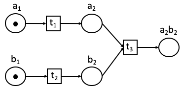
Figure 1: Causal Reversibility

For example consider the Petri net in Figure 1. We may observe that transitions $t_{\_}1$ and $t_{\_}2$ are independent from each other as they may be taken in any order, and they are both prerequisites for transition $t_{\_}3$. Backtracking the sequence of transitions $\langle t_{\_}1,t_{\_}2,t_{\_}3\rangle$ would require that the three transitions should be reversed in exactly the reverse order, i.e. $\langle t_{\_}3,t_{\_}2,t_{\_}1\rangle$. Instead, causal flexibility allows the inverse computation to rewind $t_{\_}3$ and then $t_{\_}1$ and $t_{\_}2$ in any order, but never $t_{\_}1$ or $t_{\_}2$ before $t_{\_}3$.

Both backtracking and causal reversing are cause-respecting. There are, however, many important examples where concurrent systems violate causality since undoing things in an out-of-causal order is either inherent or could be beneficial, e.g., biochemical reactions or mechanisms driving long-running transactions. This is due to the distinguishing characteristic of out-of-causal-order reversibility to allow a system to discover states that are inaccessible in any forward-only execution. This can be achieved since, reversing in out-of-causal order allows reversing an action before its effects are undone and subsequently exploring new computations while the effects of the reversed action are still present. As such, out-of-order reversibility can create fresh alternatives of current states that were formerly inaccessible by any forward-only execution path.

Since out-of-order reversibility contradicts program order, it comes with its own peculiarities that need to be taken into consideration while designing reversible systems. To appreciate these peculiarities and obtain insights towards our approach on addressing reversibility within Petri nets, consider the process of catalysis from biochemistry, whereby a substance called catalyst enables a chemical reaction between a set of other elements. Specifically consider a catalyst $c$ that helps the otherwise inactive molecules $a$ and $b$ to bond. This is achieved as follows: catalyst $c$ initially bonds with $a$ which then enables the bonding between $a$ and $b$. Finally, the catalyst is no longer needed and its bond to the other two molecules is released. A Petri net model of this process is illustrated in Figure 2. The Petri net executes transition $t_{\_}1$ via which the bond $ca$ is created, followed by action $t_{\_}2$ to produce $cab$. Finally, action $\underline{t_{\_}1}$ “reverses” the bond between $a$ and $c$, yielding $ab$ and releasing $c$. (The figure portrays the final state of the execution assuming that initially exactly one token existed in places $a$, $b$, and $c$.)

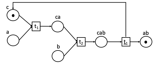
Figure 2: Catalysis in classic Petri nets

This example illustrates that Petri nets are not reversible by nature, in the sense that every transition cannot be executed in both directions. Therefore an inverse action, (e.g., transition $\underline{t_{\_}1}$ for undoing the effect of transition $t_{\_}1$) needs to be added as a supplementary forward transition for achieving the undoing of a previous action. This explicit approach of modelling reversibility can prove cumbersome in systems that express multiple reversible patterns of execution, resulting in larger and more intricate systems. Furthermore, it fails to capture reversibility as a mode of computation. The intention of our work is to study an approach for modelling reversible computation that does not require the addition of new, reversed transitions but instead offers as a basic building block transitions that can be taken in both the forward as well as the backward direction, and, thereby, explore the theory of reversible computation within Petri nets.

However, when attempting to model the catalysis example while executing transitions in both the forward and the backward directions, we may observe a number of obstacles. At an abstract level, the behaviour of the system should exhibit a sequence of three transitions: execution of $t_{\_}1$ and $t_{\_}2$, followed by the reversal of transition $t_{\_}1$. The reversal of transition $t_{\_}1$ should implement the release of $c$ from the bond $cab$ and make it available for further instantiations of transitions, if needed, while the bond $ab$ should remain in place. This implies that a reversing Petri net model should provide resources $a$, $b$ and $c$ as well as $ca$, $cab$ and $ab$ and implement the reversal of action $t_{\_}1$ as the transformation of resource $cab$ into $c$ and $ab$. Note that resource $ab$ is inaccessible during the forward execution of transitions $t_{\_}1$ and $t_{\_}2$ and only materialises after the reversal of transition $t_{\_}1$, i.e., only once the bond between $a$ and $c$ is broken. Given the static nature of a Petri net, this suggests that resources such as $ab$ should be represented at the token level (as opposed to the place level). As a result, the concept of token individuality is of particular relevance to reversible computation in Petri nets while other constructs/functions at token level are needed to capture the effect and reversal of a transition.

Indeed, reversing a transition in an out-of-causal order may imply that while some of the effects of the transition can be reversed (e.g., the release of the catalyst back to the initial state), others must be retained due to computation that succeeded the forward execution of the next transition (e.g., token $a$ cannot be released during the reversal of $t_{\_}1$ since it has bonded with $b$ in transition $t_{\_}2$). This latter point is especially challenging since it requires to specify a model in a precise manner so as to identify which effects are allowed to be “undone” when reversing a transition. Thus, as highlighted by the catalysis example, reversing transitions in a Petri net model requires close monitoring of token manipulation within a net and clear enunciation of the effects of a transition.

As already mentioned, the concept of token individuality can prove useful to handle these challenges. This concept has also been handled in various works, e.g., [31, 30, 28], where each token is associated with information regarding its causal path, i.e., the places and transitions it has traversed before reaching its current state. In our approach, we also implement the notion of token individuality where instead of maintaining extensive histories for recording the precise evolution of each token through transitions and places, we employ a novel approach inspired by out-of-causal reversibility in biochemistry as well as approaches from related literature [25]. The resulting framework is light in the sense that no memory needs to be stored per token to retrieve its causal path while enabling reversible semantics for the three main types of reversibility. Specifically, we introduce two notions that intuitively capture tokens and their history: the notion of a base and a new type of tokens called bonds. A base is a persistent type of token which cannot be consumed and therefore preserves its individuality through various transitions. For a transition to fire, the incoming arcs identify the required tokens/bonds and the outgoing arcs may create new bonds or transfer already existing tokens/bonds along the places of a PN. Therefore, the effect of a transition is the creation of new bonds between the tokens it takes as input and the reversal of such a transition involves undoing the respective bonds. In other words, a token can be a base or a coalition of bases connected via bonds into a structure.

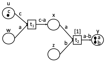
Figure 3: Catalysis in reversing Petri nets

Based on these ideas, we may describe the catalysis example in our proposed framework as shown in Figure 3. In this setting $a$, and $c$ are bases which are connected via a bond into place $x$ during transition $t_{\_}1$, while transition $t_{\_}2$ brings into place a new bond between $a$ and $b$. In Figure 3 we see the state that arises after the execution of $t_{\_}1$ and $t_{\_}2$ and the reversal of transition $t_{\_}1$. In this state, base $c$ has returned to its initial place $u$ whereas bond $a-b$ has remained in place $y$. A thorough explanation of the notation is given in the next section.

Finally, in order to identify at each point in time the history of execution, thus to discern the transitions that can be reversed given the presence of backward nondeterminism of Petri nets, we associate transitions with a history storing keys in increasing order each time an instance of the transition is executed. This allows to backtrack computation as well as to extract the causes of bonds as needed in causal and out-of-causal-order reversibility.

3 Reversing Petri Nets

We define reversing Petri nets as follows:

Definition 1.

A reversing Petri net (RPN) is a tuple $(A,P,B,T,F)$ where:

1. $A$ is a finite set of bases or tokens ranged over by $a$, $b$, $\ldots$ $\overline{A}=\{\overline{a}\mid a\in A\}$ contains a negative instance for each token and we write ${\cal{A}}=A\cup\overline{A}$.

2. $P$ is a finite set of places.

3. $B\subseteq A\times A$ is a set of undirected bonds ranged over by $\beta$, $\gamma$, $\ldots$ We use the notation $a\!-\!b$ for a bond $(a,b)\in B$. $\overline{B}=\{\overline{\beta}\mid\beta\in B\}$ contains a negative instance for each bond and we write ${\cal{B}}=B\cup\overline{B}$.

4. $T$ is a finite set of transitions.

5. $F:(P\times T\cup T\times P)\rightarrow 2^{{\cal{A}}\cup{\cal{B}}}$ defines a set of directed arcs each associated with a subset of ${\cal{A}}\cup{\cal{B}}$.

A reversing Petri net is built on the basis of a set of bases or tokens. We consider each token to have a unique name. In this way, tokens may be distinguished from each other, their persistence can be guaranteed and their history inferred from the structure of a Petri net (as implemented by function $F$, discussed below). Tokens correspond to the basic entities that occur in a system. They may occur as stand-alone elements but they may also merge together to form bonds. Places and transitions have the standard meaning.

Directed arcs connect places to transitions and vice versa and are labelled by a subset of ${\cal{A}}\cup{\cal{B}}$ where $\overline{A}=\{\overline{a}\mid a\in A\}$ is the set of negative tokens expressing token absence, and $\overline{B}=\{\overline{\beta}\mid\beta\in B\}$ is the set of negative bonds expressing bond absence. For a label $\ell=F(x,t)$ or $\ell=F(t,x)$, we assume that each token $a$ can appear in $\ell$ at most once, either as $a$ or as $\overline{a}$, and that if a bond $(a,b)\in\ell$ then $a,b\in\ell$. Furthermore, for $\ell=F(t,x)$, it must be that $\ell\cap(\overline{A}\cup\overline{B})=\emptyset$, that is, negative tokens/bonds may only occur on arcs incoming to a transition. Intuitively, these labels express the requirements for a transition to fire when placed on arcs incoming the transition, and the effects of the transition when placed on the outgoing arcs. Thus, if $a\in F(x,t)$ this implies that token $a$ is required for the transition $t$ to fire, and similarly for a bond $\beta\in F(x,t)$. On the other hand, $\overline{a}\in F(x,t)$ expresses that token $a$ should not be present in the incoming place $x$ of $t$ for the transition to fire and similarly for a bond $\beta$, $\overline{\beta}\in F(x,t)$. Note that negative tokens/bonds are close in spirit to the inhibitor arcs of extended Petri nets. Finally, note that $F(x,t)=\emptyset$ implies that there is no arc from place $x$ to transition $t$ and similarly for $F(t,x)=\emptyset$.

We introduce the following notations. We write $\circ t=\{x\in P\mid F(x,t)\neq\emptyset\}$ and $t\circ=\{x\in P\mid F(t,x)\neq\emptyset\}$ for the incoming and outgoing places of transition $t$, respectively. Furthermore, we write $\mathsf{pre}(t)=\bigcup_{\_}{x\in P}F(x,t)$ for the union of all labels on the incoming arcs of transition $t$, and $\mathsf{post}(t)=\bigcup_{\_}{x\in P}F(t,x)$ for the union of all labels on the outgoing arcs of transition $t$.

Definition 2.

A reversing Petri net $(A,P,B,T,F)$ is well-formed if it satisfies the following conditions for all $t\in T$:

1. $A\cap\mathsf{pre}(t)=A\cap\mathsf{post}(t)$,

2. If $a\!-\!b\in\mathsf{pre}(t)$ then $a\!-\!b\in\mathsf{post}(t)$,

3. $F(t,x)\cap F(t,y)=\emptyset$ for all $x,y\in P$, $x\neq y$.

According to the above we have that: (1) transitions do not erase tokens, (2) transitions do not destroy bonds, that is, if a bond $a\!-\!b$ exists in an input place of a transition, then it is maintained in some output place, and (3) tokens/bonds cannot be cloned into more than one outgoing place.

As with standard Petri nets, we employ the notion of a marking. A marking is a distribution of tokens and bonds across places, $M:P\rightarrow 2^{A\cup B}$ where $a\!-\!b\in M(x)$, for some $x\in P$, implies $a,b\in M(x)$. In addition, we employ the notion of a history, which assigns a memory to each transition of a reversing Petri net as $H:T\rightarrow 2^{\mathbb{N}}$. Intuitively, a history of $H(t)=\emptyset$ for some $t\in T$ captures that the transition has not taken place, and a history of $H(t)=\{k_{\_}1,\ldots,k_{\_}n\}$ captures that the transition was executed and not reversed $n$ times where $k_{\_}i$, $1\leq i\leq n$, indicates the order of execution of the $i^{th}$ instance amongst non-reversed actions. Note that this machinery, extending the exposition of [21], is needed to accommodate the presence of cycles, which yield the possibility of repeatedly executing the same transitions. $H_{\_}0$ denotes the initial history where $H_{\_}0(t)=\emptyset$ for all $t\in T$. A pair of a marking and a history describes a state of a PN based on which execution is determined. We use the notation $\langle{M},{H}\rangle$ to denote states.

In a graphical representation, tokens are indicated by $\bullet$, places by circles, transitions by boxes, and bonds by lines between tokens. Furthermore, histories are presented over the respective transitions as the list $[k_{\_}1,...,k_{\_}n]$ when $H(t)=\{k_{\_}1,\ldots,k_{\_}n\}$, $n>0$, and omitted when $H(t)=\emptyset$.

As the last piece of our machinery, we define a notion that identifies connected components of tokens and their associated bonds within a place. Note that more than one connected component may arise in a place due to the fact that various unconnected tokens may be moved to a place simultaneously by a transition, while the reversal of transitions, which results in the destruction of bonds, may break down a connected component into various subcomponents. We define $\mathsf{con}(a,C)$, where $a$ is a base and $C\subseteq A\cup B$ to be the tokens connected to $a$ via sequences of bonds as well as the bonds creating these connections according to set $C$.

$$\mathsf{con}(a,C)=(\{a\}\cap C)\cup\{\beta,b,c\mid\exists w\mbox{ s.t. }\mathsf{path}(a,w,C),\beta\in w\mbox{, and }\beta=(b,c)\}$$

where $\mathsf{path}(a,w,C)$ if $w=\langle\beta_{\_}1,\ldots,\beta_{\_}n\rangle$, and for all $1\leq i\leq n$, $\beta_{\_}i=(a_{\_}{i-1},a_{\_}i)\in C\cap B$, $a_{\_}i\in C\cap A$, and $a_{\_}0=a$.

Returning to the example of Figure 3, we may see a reversing net with three tokens $a$, $b$, and $c$, transition $t_{\_}1$, which bonds tokens $a$ and $c$ within place $x$, and transition $t_{\_}2$, which bonds the $a$ of bond $c\!-\!a$ with token $b$ into place $y$. Note that to avoid overloading figures, we omit writing the bases of bonds on the arcs of RPNs, so, e.g., on the arc between $t_{\_}1$ and $x$, we write $a\!-\!b$ as opposed to $\{a\!-\!b,a,b\}$. (The marking depicted in the figure is the one arising after the execution of transitions $t_{\_}1$ and $t_{\_}2$ and subsequently the reversal of transition $t_{\_}1$ by the semantic relations to be defined in the next section.)

We may now define the various types of execution for reversing Petri nets. In what follows we restrict our attention to well-formed RPNs $(A,P,B,T,F)$ with initial marking $M_{\_}0$ such that for all $a\in A$, $|\{x\mid a\in M_{\_}0(x)\}|=1$.

4 Forward Execution

In this section we consider the standard, forward execution of RPNs.

Definition 3.

Consider a reversing Petri net $(A,P,B,T,F)$, a transition $t\in T$, and a state $\langle{M},{H}\rangle$. We say that $t$ is forward-enabled in $\langle{M},{H}\rangle$ if the following hold:

1. if $a\in F(x,t)$, for some $x\in\circ t$, then $a\in M(x)$, and if $\overline{a}\in F(x,t)$ for some $x\in\circ t$, then $a\not\in M(x)$,

2. if $\beta\in F(x,t)$, for some $x\in\circ t$, then $\beta\in M(x)$, and if $\overline{\beta}\in F(x,t)$ for some $x\in\circ t$, then $\beta\not\in M(x)$,

3. if $a\in F(t,y_{\_}1)$, $b\in F(t,y_{\_}2)$, $y_{\_}1\neq y_{\_}2$, then $b\not\in\mathsf{con}(a,M(x))$ for all $x\in\circ t$, and

4. if $\beta\in F(t,x)$ for some $x\in t\circ$ and $\beta\in M(y)$ for some $y\in\circ t$, then $\beta\in F(y,t)$.

Thus, $t$ is enabled in state $\langle{M},{H}\rangle$ if (1), (2), all tokens and bonds required for the transition to take place are available in the incoming places of $t$ and none of the tokens/bonds whose absence is required exists in an incoming place of the transition, (3) if a transition forks into outgoing places $y_{\_}1$ and $y_{\_}2$ then the tokens transferred to these places are not connected to each other in the incoming places of the transition, and (4) if a pre-existing bond appears in an outgoing arc of a transition, then it is also a precondition of the transition to fire. Contrariwise, if the bond appears in an outgoing arc of a transition ($\beta\in F(t,x)$ for some $x\in t\circ$) but is not a requirement for the transition to fire ($\beta\not\in F(y,t)$ for all $y\in\circ t$), then the bond should not be present in an incoming place of the transition ($\beta\not\in M(y)$ for all $y\in\circ t$).

We observe that the new bonds created by a transition are exactly those that occur in the outgoing edges of a transition but not in the incoming edges. Thus, we define the effect of a transition as

$$\mathsf{eff}(t)=\mathsf{post}(t)-\mathsf{pre}(t)$$

This will subsequently enable the enunciation of transition reversal by the destruction of exactly the bonds in $\mathsf{eff}(t)$.

Definition 4.

Given a reversing Petri net $(A,P,B,T,F)$, a state $\langle M,H\rangle$, and a transition $t$ enabled in $\langle{M},{H}\rangle$, we write $\langle{M},{H}\rangle\stackrel{{\scriptstyle t}}{{\longrightarrow}}\langle{M^{\prime}},{H^{\prime}}\rangle$ where:

$$\begin{array}[]{rcl}M^{\prime}(x)&=&\left\{\begin{array}[]{ll}M(x)-\bigcup_{\_}{a\in F(x,t)}\mathsf{con}(a,M(x))&\textrm{if }x\in\circ{t}\\ M(x)\cup F(t,x)\cup\bigcup_{\_}{a\in F(t,x)\cap F(y,t)}\mathsf{con}(a,M(y))&\textrm{if }x\in t\circ\\ M(x),&\textrm{otherwise}\end{array}\right.\end{array}$$

and

$$\begin{array}[]{rcl}H^{\prime}(t^{\prime})&=&\left\{\begin{array}[]{lll}H(t^{\prime})\cup\{\max(\{0\}\cup\{k\mid k\in H(t^{\prime\prime}),t^{\prime\prime}\in T\})+1\},\hskip 7.22743pt\textrm{if }t^{\prime}=t\\ H(t^{\prime}),\hskip 216.81pt\textrm{ otherwise}\end{array}\right.\end{array}$$

Thus, when a transition $t$ is executed in the forward direction, all tokens and bonds occurring in its incoming arcs are relocated from the input places to the output places along with their connected components. An example of forward transitions can be seen in Figure  4 where transitions $t_{\_}1$ and $t_{\_}2$ take place with the histories of the two transitions becoming $[1]$ and $[2]$, respectively.

Figure 4: Forward execution

We may prove the following result, which verifies that bases are preserved during forward execution in the sense that transitions neither erase nor clone them. As far as bonds are concerned, the proposition states that forward execution may create but not destroy bonds.

Proposition 1 (Token and bond preservation).

Consider a reversing Petri net $(A,P,B,T,F)$, a state $\langle M,H\rangle$ such that for all $a\in A$, $|\{x\in P\mid a\in M(x)\}|=1$, and a transition $\langle{M},{H}\rangle\stackrel{{\scriptstyle t}}{{\longrightarrow}}\langle{M^{\prime}},{H^{\prime}}\rangle$. Then:

1. for all $a\in A$, $|\{x\in P\mid a\in M^{\prime}(x)\}|=1$, and

2. for all $\beta\in B$, $|\{x\in P\mid\beta\in M(x)\}|\leq|\{x\in P\mid\beta\in M^{\prime}(x)\}|\leq 1$.

Proof:

The proof of the result follows the definition of forward execution and relies on the well-formedness of RPNs. Consider a reversing Petri net $(A,P,B,T,F)$, a state $\langle M,H\rangle$ such that $|\{x\in P\mid a\in M(x)\}|=1$ for all $a\in A$, and suppose $\langle{M},{H}\rangle\stackrel{{\scriptstyle t}}{{\longrightarrow}}\langle{M^{\prime}},{H^{\prime}}\rangle$.

For the proof of clause (1) let $a\in A$. Two cases exist:

1. $a\in\mathsf{con}(b,M(x))$ for some $b\in F(x,t)$. Note that $x$ is unique by the assumption that $|\{x\in P\mid a\in M(x)\}|=1$. Furthermore, according to Definition 4, we have that $M^{\prime}(x)=M(x)-\{\mathsf{con}(b,M(x))\mid b\in F(x,t)\}$, which implies that $a\not\in M^{\prime}(x)$. On the other hand, by Definition 2(1), $b\in\mathsf{post}(t)$. Thus, there exists $y\in t\circ$, such that $b\in F(t,y)$. Note that this $y$ is unique by Definition 2(3). As a result, by Definition 4, $M^{\prime}(y)=M(y)\cup F(t,y)\cup\{\mathsf{con}(b,M(x))\mid b\in F(t,y),x\in\circ{t}\}$. Since $b\in F(x,t)\cap F(t,y)$, $a\in\mathsf{con}(b,M(x))$, this implies that $a\in M^{\prime}(y)$.

   Now suppose that $a\in\mathsf{con}(c,M(x))$ for some $c\neq b$, $c\in F(t,y^{\prime})$. Then, by Definition 3(3), it must be that $y=y^{\prime}$. As a result, we have that $\{z\in P\mid a\in M^{\prime}(z)\}=\{y\}$ and the result follows.

2. $a\not\in\mathsf{con}(b,M(x))$ for all $b\in F(x,t)$, $x\in P$. This implies that $\{x\in P\mid a\in M^{\prime}(x)\}=\{x\in P\mid a\in M(x)\}$ and the result follows.

To prove clause (2) of the proposition, consider a bond $\beta\in B$, $\beta=(a,b)$. We observe that, since $|\{x\in P\mid a\in M(x)\}|=1$ for all $a\in A$, $|\{x\in P\mid\beta\in M(x)\}|\leq 1$. The proof follows by case analysis as follows:

1. Suppose $|\{x\in P\mid\beta\in M(x)\}|=0$. Two cases exist:

   • Suppose $\beta\not\in F(t,x)$ for all $x\in P$. Then, by Definition 4, $\beta\not\in M^{\prime}(x)$ for all $x\in P$. Consequently, $|\{x\in P\mid\beta\in M^{\prime}(x)\}|=0$ and the result follows.

   • Suppose $\beta\in F(t,x)$ for some $x\in P$. Then, by Definition 2(3), $x$ is unique, and by Definition 4, $\beta\in M^{\prime}(x)$. Consequently, $|\{x\in P\mid\beta\in M^{\prime}(x)\}|=1$ and the result follows.

2. Suppose $|\{x\in P\mid\beta\in M(x)\}|=1$. Two cases exist:

   • $\beta\not\in\mathsf{con}(c,M(x))$ for all $c\in F(x,t)$. This implies that $\{x\in P\mid\beta\in M^{\prime}(x)\}=\{x\in P\mid\beta\in M(x)\}$ and the result follows.

   • $\beta\in\mathsf{con}(c,M(x))$ for some $c\in F(x,t)$. Then, according to Definition 4, we have that $M^{\prime}(x)=M(x)-\{\mathsf{con}(c,M(x))\mid c\in F(x,t)\}$, which implies that $\beta\not\in M^{\prime}(x)$. On the other hand, by the definition of well-formedness, Definition 2(1), $c\in\mathsf{post}(t)$. Thus, there exists $y\in t\circ$, such that $c\in F(t,y)$. Note that this $y$ is unique by Definition 2(3). As a result, by Definition 4, $M^{\prime}(y)=M(y)\cup F(t,y)\cup\{\mathsf{con}(c,M(x))\mid c\in F(t,y),x\in\circ{t}\}$. Since $c\in F(x,t)\cap F(t,y)$, $\beta\in\mathsf{con}(c,M(x))$, this implies that $\beta\in M^{\prime}(y)$.

     Now suppose that $\beta\in\mathsf{con}(d,M(x))$ for some $d\neq c$, $c\in F(d,y^{\prime})$. Then, by Definition 3, and since $\mathsf{con}(c,M(x))=\mathsf{con}(d,M(x))$, it must be that $y=y^{\prime}$. As a result, we have that $\{z\in P\mid\beta\in M^{\prime}(z)\}=\{y\}$ and the result follows.

   $\Box$

5 Reverse Execution

5.1 Backtracking

Let us now proceed to the simplest form of reversibility, namely, backtracking. We define a transition to be bt-enabled (backtracking-enabled) if it was the last executed transition:

Definition 5.

Consider a state $\langle{M},{H}\rangle$ and a transition $t\in T$. We say that $t$ is $bt$-enabled in $\langle{M},{H}\rangle$ if $k\in H(t)$ with $k\geq k^{\prime}$ for all $k^{\prime}\in H(t^{\prime})$, $t^{\prime}\in T$.

Thus, a transition $t$ is $bt$-enabled if its history contains the highest value among all transitions. The effect of backtracking a transition in a reversing Petri net is as follows:

Definition 6.

Given a reversing Petri net $(A,P,B,T,F)$, a state $\langle M,H\rangle$, and a transition $t$ that is $bt$-enabled in $\langle{M},{H}\rangle$, we write $\langle{M},{H}\rangle\stackrel{{\scriptstyle t}}{{\rightsquigarrow}}_{b}\langle{M^{\prime}},{H^{\prime}}\rangle$ where:

$$\begin{array}[]{rcl}M^{\prime}(x)&=&\left\{\begin{array}[]{ll}M(x)\cup\bigcup_{\_}{y\in t\circ,a\in F(x,t)\cap F(t,y)}\mathsf{con}(a,M(y)-\mathsf{eff}(t)),&\textrm{if }x\in\circ{t}\\ M(x)-\bigcup_{\_}{a\in F(t,x)}\mathsf{con}(a,M(x)),&\textrm{if }x\in t\circ\\ M(x)&\textrm{otherwise}\end{array}\right.\end{array}$$

and

$$\begin{array}[]{rcl}H^{\prime}(t^{\prime})&=&\left\{\begin{array}[]{lll}H(t^{\prime})-\{k\},&\textrm{if }t^{\prime}=t,k=\max(H(t))\\ H(t^{\prime})&\textrm{otherwise}\end{array}\right.\end{array}$$

Figure 5: Backtracking execution

When a transition $t$ is reversed in a backtracking fashion all tokens and bonds in the postcondition of the transition, as well as their connected components, are transferred to the incoming places of the transition and any newly-created bonds are broken. Furthermore, the largest key in the history of the transition is removed.

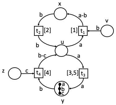
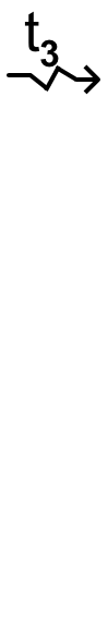
Figure 6: Backtracking execution where $\sigma=\langle t_{\_}1,t_{\_}2,t_{\_}3,t_{\_}4,t_{\_}3\rangle$

An example of backtracking extending the example of Figure 4 can be seen in Figure 5 where we observe transitions $t_{\_}2$ and $t_{\_}1$ being reversed with the histories of the two transitions being eliminated. A further example can be seen in Figure 6 where after the execution of transition sequence $\langle t_{\_}1,t_{\_}2,t_{\_}3,t_{\_}4,t_{\_}3\rangle$, only transition $t_{\_}3$ is $bt$-enabled since it was the last transition to be executed. During its reversal, the component $a\!-\!b\!-\!c$ is returned to place $u$. Furthermore, the largest key of the history of $t_{\_}3$ becomes empty.

We may prove the following result, which verifies that bases are preserved during backtracking execution in the sense that there exists exactly one instance of each base and backtracking transitions neither erase nor clone them. As far as bonds are concerned, the proposition states that at any time there may exist at most one instance of a bond and that backtracking transitions may only destroy bonds.

Proposition 2 (Token preservation and bond destruction).

Consider a reversing Petri net $(A,P,B,T,F)$, a state $\langle M,H\rangle$ such that for all $a\in A$, $|\{x\in P\mid a\in M(x)\}|=1$, and a transition $\langle{M},{H}\rangle\stackrel{{\scriptstyle t}}{{\rightsquigarrow}}_{b}\langle{M^{\prime}},{H^{\prime}}\rangle$. Then:

1. for all $a\in A$, $|\{x\in P\mid a\in M^{\prime}(x)\}|=1$, and

2. for all $\beta\in B$, $1\geq|\{x\in P\mid\beta\in M(x)\}|\geq|\{x\in P\mid\beta\in M^{\prime}(x)\}|$.

Proof:

The proof of the result follows the definition of backward execution and relies on the well-formedness of reversing Petri nets. Consider RPN $(A,P,B,T,F)$, a state $\langle M,H\rangle$ such that $|\{x\in P\mid a\in M(x)\}|=1$ for all $a\in A$, and suppose $\langle{M},{H}\rangle\stackrel{{\scriptstyle t}}{{\rightsquigarrow}}_{b}\langle{M^{\prime}},{H^{\prime}}\rangle$.

We begin with the proof of clause (1) and let $a\in A$. Two cases exist:

1. $a\in\mathsf{con}(b,M(x))$ for some $b\in F(t,x)$. Note that by the assumption of $|\{x\in P\mid a\in M(x)\}|=1$, $x$ must be unique. Let us choose $b$ such that, additionally, $a\in\mathsf{con}(b,M(x)-\mathsf{eff}(t))$. Note that such a $b$ must exist, otherwise the forward execution of $t$ would not have transferred $a$ along with $b$ to place $x$.

   According to Definition 6, we have that $M^{\prime}(x)=M(x)-\{\mathsf{con}(b,M(x))\mid b\in F(t,x)\}$, which implies that $a\not\in M^{\prime}(x)$. On the other hand, note that by the definition of well-formedness, Definition 2(1), $b\in\mathsf{pre}(t)$. Thus, there exists $y\in\circ t$, such that $b\in F(y,t)$. Note that this $y$ is unique. If not, then there exist $y$ and $y^{\prime}$ such that $y\neq y^{\prime}$ with $b\in F(y,t)$ and $b\in F(y^{\prime},t)$. By the assumption, however, that there exists at most one token of each base, and Proposition 1, $t$ would never be enabled, which leads to a contradiction. As a result, by Definition 6, $M^{\prime}(y)=M(y)\cup\{\mathsf{con}(b,M(x)-\mathsf{eff}(t))\mid b\in F(y,t)\cap F(t,x)\}$. Since $b\in F(y,t)\cap F(t,x)$, $a\in\mathsf{con}(b,M(x)-\mathsf{eff}(t))$, this implies that $a\in M^{\prime}(y)$.

   Now suppose that $a\in\mathsf{con}(c,M(x)-\mathsf{eff}(t))$, $c\neq b$, and $c\in F(y^{\prime},t)$. Since $a\in\mathsf{con}(b,M(x)-\mathsf{eff}(t))$, it must be that $\mathsf{con}(b,M(x)-\mathsf{eff}(t))=\mathsf{con}(c,M(x)-\mathsf{eff}(t))$. Since $b$ and $c$ are connected to each other but the connection was not created by transition $t$ (the connection is present in $M(x)-\mathsf{eff}(t)$), it must be that the connection was already present before the forward execution of $t$ and, by token uniqueness, we conclude that $y=y^{\prime}$.

2. $a\not\in\mathsf{con}(b,M(x))$ for all $b\in F(t,x)$, $x\in P$. This implies that $\{x\in P\mid a\in M^{\prime}(x)\}=\{x\in P\mid a\in M(x)\}$ and the result follows.

Let us now prove clause (2) of the proposition. Consider a bond $\beta\in B$, $\beta=(a,b)$. We observe that, since $|\{x\in P\mid a\in M(x)\}|=1$ for all $a\in A$, $|\{x\in P\mid\beta\in M(x)\}|\leq 1$. The proof follows by case analysis as follows:

1. $\beta\in\mathsf{con}(c,M(x))$ for some $c\in F(t,x)$, $x\in P$. By the assumption of $|\{x\in P\mid\beta\in M(x)\}|=1$, $x$ must be unique. Then, according to Definition 6, we have that $M^{\prime}(x)=M(x)-\{\mathsf{con}(c,M(x))\mid c\in F(x,t)\}$, which implies that $\beta\not\in M^{\prime}(x)$. Two cases exist:

   • If $\beta\in\mathsf{eff}(t)$, then $\beta\not\in M^{\prime}(y)$ for all places $y\in P$.

   • If $\beta\not\in\mathsf{eff}(t)$ then let us choose $c$ such that $\beta\in\mathsf{con}(c,M(x)-\mathsf{eff}(t))$. Note that such a $c$ must exist, otherwise the forward execution of $t$ would not have connected $\beta$ with $c$. By the definition of well-formedness, Definition 2(1), $c\in\mathsf{pre}(t)$. Thus, there exists $y\in\circ t$, such that $c\in F(y,t)$. Note that this $y$ is unique (if not, $t$ would not have been enabled). As a result, by Definition 6, $\beta\in M^{\prime}(y)$.

     Now suppose that $\beta\in\mathsf{con}(d,M(x)-\mathsf{eff}(t))$, $d\neq c$, and $d\in M^{\prime}(y^{\prime})$. Since $\beta\in\mathsf{con}(c,M(x)-\mathsf{eff}(t))$, it must be that $\mathsf{con}(c,M(x)-\mathsf{eff}(t))=\mathsf{con}(d,M(x)-\mathsf{eff}(t))$. Since $c$ and $d$ are connected to each other but the connection was not created by transition $t$ (the connection is present in $M(x)-\mathsf{eff}(t)$), it must be that the connection was already present before the forward execution of $t$ and, by token uniqueness, we conclude that $y=y^{\prime}$. This implies that $\{z\in P\mid\beta\in M^{\prime}(z)\}=\{y\}$.

   The above imply that $\{z\in P\mid\beta\in M(z)\}=\{x\}$ and $\{z\in P\mid\beta\in M^{\prime}(z)\}\subseteq\{y\}$ and the result follows.

2. $\beta\not\in\mathsf{con}(c,M(x))$ for all $c\in F(t,x)$, $x\in P$. This implies that $\{x\in P\mid\beta\in M^{\prime}(x)\}=\{x\in P\mid\beta\in M(x)\}$ and the result follows. $\Box$

Let us now consider the combination of forward and backward moves in executions. We write $\stackrel{{\scriptstyle}}{{\longmapsto}}_{b}$ for $\stackrel{{\scriptstyle}}{{\longrightarrow}}\cup\stackrel{{\scriptstyle}}{{\rightsquigarrow}}_{b}$. The following result establishes that in an execution beginning in the initial state of a reversing Petri net, bases are preserved, bonds can have at most one instance at any time and a new occurrence of a bond may be created during a forward transition that features the bond as its effect whereas a bond can be destroyed during the backtracking of a transition that features the bond as its effect. This last point clarifies that the effect of a transition characterises the bonds that are newly-created during the transition’s forward execution and the ones that are destroyed during its reversal.

Proposition 3.

Given a reversing Petri net $(A,P,B,T,F)$, an initial state $\langle M_{\_}0,H_{\_}0\rangle$ and an execution $\langle{M_{\_}0},{H_{\_}0}\rangle\stackrel{{\scriptstyle t_{\_}1}}{{\longmapsto}}_{b}\langle{M_{\_}1},{H_{\_}1}\rangle\stackrel{{\scriptstyle t_{\_}2}}{{\longmapsto}}_{b}\ldots\stackrel{{\scriptstyle t_{\_}n}}{{\longmapsto}}_{b}\langle{M_{\_}n},{H_{\_}n}\rangle$, the following hold:

1. For all $a\in A$ and $i$, $0\leq i\leq n$, $|\{x\in P\mid a\in M_{\_}i(x)\}|=1$.

2. For all $\beta\in B$ and $i$, $0\leq i\leq n$,

   1. $0\leq|\{x\in P\mid\beta\in M_{\_}i(x)\}|\leq 1$,

   2. if $t_{\_}i$ is executed in the forward direction and $\beta\in\mathsf{eff}(t_{\_}i)$, then $\beta\in M_{\_}{i}(x)$ for some $x\in P$ where $\beta\in F(t_{\_}i,x)$, and $\beta\not\in M_{\_}{i-1}(y)$ for all $y\in P$,

   3. if $t_{\_}i$ is executed in the forward direction, $\beta\in M_{\_}{i-1}(x)$ for some $x\in P$, and $\beta\not\in\mathsf{eff}(t_{\_}i)$ then, if $\beta\in\mathsf{con}(a,M_{\_}{i-1}(x))$ and $a\in F(t_{\_}i,y)$, then $\beta\in M_{\_}{i}(y)$, otherwise $\beta\in M_{\_}i(x)$,

   4. if $t_{\_}i$ is executed in the reverse direction and $\beta\in\mathsf{eff}(t_{\_}i)$ then $\beta\in M_{\_}{i-1}(x)$ for some $x\in P$ where $\beta\in F(t_{\_}i,x)$, and $\beta\not\in M_{\_}{i}(y)$ for all $y\in P$, and

   5. if $t_{\_}i$ is executed in the reverse direction, $\beta\in M_{\_}{i-1}(x)$ for some $x\in P$, and $\beta\not\in\mathsf{eff}(t_{\_}i)$ then, if $\beta\in\mathsf{con}(a,M_{\_}{i-1}(x))$ and $a\in F(y,t_{\_}i)$, then $\beta\in M_{\_}{i}(y)$, otherwise $\beta\in M_{\_}i(x)$.

Proof:

To begin with, we observe that the proofs of clauses (1) and (2)(a) follow directly from clauses (1) and (2) of Propositions 1 and 2. Clause (2)(b) follows from Definition 3(4) and Definition 4. Clause (2)(c) follows from Definition 4 and the condition refers to whether the bond is part of a component manipulated by the forward execution of $t_{\_}i$. Similarly,to (2)(a) clause (2)(d) stems from Definition 6. Finally, Clause (2)(e) follows from Definition 6 and the condition refers to whether the bond is part of a component manipulated by the reverse execution of $t_{\_}i$. $\Box$

In this setting we may establish a loop lemma:

Lemma 1 (Loop).

For any forward transition $\langle{M},{H}\rangle\stackrel{{\scriptstyle t}}{{\longrightarrow}}\langle{M^{\prime}},{H^{\prime}}\rangle$ there exists a backward transition $\langle{M^{\prime}},{H^{\prime}}\rangle\stackrel{{\scriptstyle t}}{{\rightsquigarrow}}_{b}\langle{M},{H}\rangle$ and vice versa.

Proof:

Suppose $\langle{M},{H}\rangle\stackrel{{\scriptstyle t}}{{\longrightarrow}}\langle{M^{\prime}},{H^{\prime}}\rangle$. Then $t$ is clearly $bt$-enabled in $H^{\prime}$. Furthermore, $\langle{M^{\prime}},{H^{\prime}}\rangle\stackrel{{\scriptstyle t}}{{\rightsquigarrow}}_{b}\langle{M^{\prime\prime}},{H^{\prime\prime}}\rangle$ where $H^{\prime\prime}=H$. In addition, all tokens and bonds involved in transition $t$ (except those in $\mathsf{eff}(t)$) will be returned from the outgoing places of transition $t$ back to its incoming places. Specifically, for all $a\in A$, it is easy to see by the definition of $\stackrel{{\scriptstyle}}{{\rightsquigarrow}}_{b}$ that $a\in M^{\prime\prime}(x)$ if and only if $a\in M(x)$. Similarly, for all $\beta\in B$, $\beta\in M^{\prime\prime}(x)$ if and only if $\beta\in M(x)$. The opposite direction can be argued similarly. $\Box$

5.2 Causal-order reversibility

We now move on to consider causal-order reversibility in RPNs. To define such as reversible semantics in the presence of cycles, a number of issues need to be resolved. To begin with, consider a sequence of transitions pertaining to the repeated execution of a cycle. Adopting the view that reversible computation has the ability to rewind every executed action of a system, we require that each of these transitions is executed in reverse as many times as it was executed in the forward direction. Furthermore, the presence of cycles raises questions about the causal relationship between transitions of a cycle as well as of overlapping or even structurally distinct cycles. In the next subsection we discuss our adopted notion of transition causality. Subsequently, we develop a theory for causal-order reversibility in RPNs.

5.2.1 Causality in cyclic reversing Petri nets

A cycle in a reversing Petri net is associated with a cyclic path in the net’s graph structure. It contains a sequence of transitions where an outgoing place of the last transition coincides with an incoming place of the first transition. Note that a cycle in the graph of a reversing Petri net does not necessarily imply the repeated execution of its transitions since, for instance, entrance to the cycle may require a token or a bond that has been directed into a different part of the net during execution of the cycle.

In the standard approach to causality in classical Petri nets [26], a causal link is considered to exist between two transitions if one produces tokens that are used to fire the other. This relation is used to define a “causal order”, $\prec$, which is transitive so that if a transition $t_{\_}1$ causally precedes $t_{\_}2$ and $t_{\_}2$ causally precedes $t_{\_}3$, then $t_{\_}1$ also causally precedes $t_{\_}3$.

Adapting this notion in the context of cycle execution, consider a cycle with transitions $t_{\_}1$ and $t_{\_}2$, executed twice yielding the transition instances $t_{\_}1^{1}$, $t_{\_}2^{1}$, $t_{\_}1^{2}$, $t_{\_}2^{2}$, where $t_{\_}i^{j}$ denotes the $j$-th execution of transition $t_{\_}i$. Furthermore, suppose that $t_{\_}1$ produces tokens that are consumed by $t_{\_}2$ and vice versa. This implies the causal order relation $\prec$, such that $t_{\_}1^{1}\prec t_{\_}2^{1}\prec t_{\_}1^{2}\prec t_{\_}2^{2}$, allowing us to conclude that each execution of the cycle causally precedes any subsequent executions. This is a natural conclusion in the case of the consecutive execution of cycles, since a second execution of a cycle cannot be initiated before the first one is completed. This is because the tokens manipulated by the first transition of the cycle need to return to its input places before the transition can be repeated.

Let us now move on to determining when a token produced by a transition is consumed by another. In RPNs this concept acquires an additional complexity due to the fact that tokens are distinguished by names and the fact that the creation of bonds between tokens may disguise the causal relation between transitions. For instance, consider the example of Figure 7. This RPN features two overlapping cycles, which can be executed sequentially. Suppose we execute the outer cycle (transition sequence $\langle t_{\_}1,t_{\_}2,t_{\_}3,t_{\_}4,t_{\_}5,t_{\_}6\rangle$) followed by the inner cycle (transition sequence $\langle t_{\_}1,t_{\_}2,t_{\_}7,t_{\_}6\rangle$).

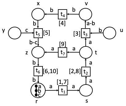
Figure 7: RPN with overlapping cycles $\sigma_{\_}1=\langle t_{\_}1,t_{\_}2,t_{\_}3,t_{\_}4,t_{\_}5,t_{\_}6\rangle$ and $\sigma_{\_}2=\langle t_{\_}1,t_{\_}2,t_{\_}7,t_{\_}6\rangle$, and the state arising after the forward execution of $\sigma=\sigma_{\_}1\sigma_{\_}2$

Observing the token manipulation of the transition instances as captured by the arcs of the transition, we obtain the order $t_{\_}1^{1}\prec t_{\_}2^{1}\prec t_{\_}3^{1}\prec t_{\_}4^{1}\prec t_{\_}5^{1}\prec t_{\_}6^{1}$ and $t_{\_}1^{2}\prec t_{\_}2^{2}\prec t_{\_}7^{1}\prec t_{\_}6^{2}$. However by simply observing the structure of the RPN there is no evidence that $t_{\_}1$ consumes tokens produced by $t_{\_}6$. Nonetheless, in this scenario transition instance $t_{\_}3^{1}$ has bonded tokens $a$ and $b$ and, thus, transition instance $t_{\_}1^{2}$ requires bond $a-b$ to be produced and placed at $r$ by $t_{\_}6$ before transition $t_{\_}1$ can be executed for the second time. Thus, $t_{\_}6^{1}\prec t_{\_}1^{2}$ also holds.

Note that, if the two cycles were not considered to be causally dependent and were allowed to reverse in any order, then, reversal of the first before the second one would disable the reversal of the second cycle. This is because reversing transition $t_{\_}3$ would return token $b$ to place $u$, thus disabling a second reversal of transition $t_{\_}6$ (and consequently the reversal of the inner cycle).

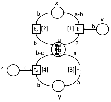
Figure 8: Causally dependent cycles, where $\sigma=\langle t_{\_}1,t_{\_}2,t_{\_}3,t_{\_}4\rangle$

Similarly, in the example of Figure 8 we observe two cycles that are structurally independent but where the presence of common tokens between the two cycles creates a dependence between their executions. For instance, suppose that the upper cycle is initially selected via execution of transition $t_{\_}1$. This choice disables the lower cycle, which is only re-enabled once the upper cycle is completed and token $a$ is returned to place $u$. As a result, the execution of $t_{\_}3$, and thus the lower cycle, following an execution of the upper cycle, is considered to be causally dependent on the execution of $t_{\_}2$.

The above examples highlight that syntactic token independence between two transitions or cycles does not preclude their causal dependence. Instead, causal dependence is determined by the path that tokens follow: two transition occurrences are causally dependent, if a token produced by the one occurrence was subsequently used to fire the other occurrence. To capture this type of dependencies, we adopt the following definitions.

Definition 7.

Consider a state $\langle{M},{H}\rangle$ and a transition $t$. We refer to $(t,k)$ as a transition occurrence in $\langle{M},{H}\rangle$ if $k\in H(t)$.

Definition 8.

Consider a state $\langle{M},{H}\rangle$ and suppose $\langle{M},{H}\rangle\stackrel{{\scriptstyle t}}{{\longrightarrow}}\langle{M^{\prime}},{H^{\prime}}\rangle$ with $(t,k)$, $(t^{\prime},k^{\prime})$ transition occurrences in $\langle{M^{\prime}},{H^{\prime}}\rangle$, $k=\max(H(t))$. We say that $(t,k)$ causally depends on $(t^{\prime},k^{\prime})$ denoted by $(t^{\prime},k^{\prime})\prec(t,k)$, if $k^{\prime}<k$ and there exists $a\in F(x,t)$ where $\mathsf{con}(a,M(x))\cap\mathsf{post}(t^{\prime})\neq\emptyset$.

Thus, a transition occurrence $(t,k)$ causally depends on a preceding transition occurrence $(t^{\prime},k^{\prime})$ if one or more tokens used during the firing of $(t,k)$ was produced by $(t^{\prime},k^{\prime})$. Note that the tokens employed during a transition in a specific marking are determined by the connected components of $F(x,t)$ in the marking. For example, in Figure 7 we have $(t_{\_}5,5)\prec(t_{\_}7,9)$ and in Figure 8 $(t_{\_}1,1)\prec(t_{\_}4,4)$, where in each case token $a$ has been transferred from its initial place through $(t_{\_}5,5)$ to $(t_{\_}7,9)$ and through $(t_{\_}1,1)$ to $(t_{\_}4,4)$, respectively.

5.2.2 Causal reversing

Following this approach to causality, we now move on to define causal-order reversibility in reversing Petri nets. As expected, we consider a transition $t$ to be enabled for causal-order reversal only if all transitions that are causally dependent on it have either been reversed or not executed. To this respect, relation $\prec$ becomes an important piece of machinery and we extend the notion of a state for the purposes of causal dependence to a triple $\langle{M},{H},{\prec}\rangle$ where $\prec$ captures the causal dependencies that have formed up to the creation of the state. We assume that in the initial state $\prec=\emptyset$ and we extend the definition of forward execution as follows:

Definition 9.

Given a reversing Petri net $(A,P,B,T,F)$, a state $\langle M,H,\prec\rangle$, and a transition $t$ forward-enabled in $\langle{M},{H}\rangle$, we write $\langle{M},{H},{\prec}\rangle\stackrel{{\scriptstyle t}}{{\longrightarrow}}\langle{M^{\prime}},{H^{\prime}},{\prec^{\prime}}\rangle$ where $M^{\prime}$ and $H^{\prime}$ are defined as in Definition 4, and

$$\prec^{\prime}\;=\;\prec\cup\{((t^{\prime},k^{\prime}),\!(t,k))\mid k\!=\!\max(H^{\prime}(t)),(t,k)\mbox{ causally depends on }(t^{\prime},k^{\prime})\}$$

We may now define that a transition is enabled for causal-order reversal as follows:

Definition 10.

Consider a state $\langle{M},{H},{\prec}\rangle$ and a transition $t\in T$. Then $t$, $H(t)\neq\emptyset$, is $co$-enabled (causal-order reversal enabled) in $\langle M,H,\prec\rangle$ if

1. for all $x\in t\circ$, if $a\in F(t,x)$ then $a\in M(x)$ and if $\beta\in F(t,x)$ then $\beta\in M(x)$, and

2. there is no transition occurrence $(t^{\prime},k^{\prime})\in\langle M,H,\prec\rangle$ with $(t,k)\prec(t^{\prime},k^{\prime})$, for $k=max(H(t))$.

According to the definition, an executed transition is $co$-enabled if all tokens and bonds required for its reversal (i.e., in $\mathsf{post}(t)$) are available in its outgoing places and there are no transitions which depend on it causally. Note that the second condition becomes relevant in the presence of cycles since it is possible that, while more than one transitions simultaneously have available the tokens required for their reversal, only one of them is $co$-enabled. Such an example can be seen in the final state of Figure 8 and transitions $t_{\_}2$ and $t_{\_}4$.

Reversing a transition in a causally-respecting manner is implemented similarly to backtracking, i.e. the tokens are moved from the outgoing places to the incoming places of the transition and all bonds created by the transition are broken. In addition, the history function is updated in the same manner as in backtracking, where we remove the key of the reversed transition. Finally, the causal dependence relation removes all references to the reversed transition occurrence.

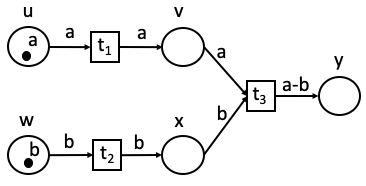
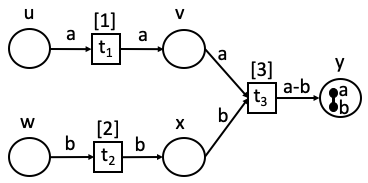
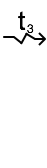
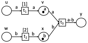
Figure 9: Causal-order example

Definition 11.

Given a state $\langle M,H,\prec\rangle$ and a transition $t$ $co$-enabled in $\langle M,H,\prec\rangle$, we write $\langle{M},{H},{\prec}\rangle\stackrel{{\scriptstyle t}}{{\rightsquigarrow}}_{c}\langle{M^{\prime}},{H^{\prime}},{\prec^{\prime}}\rangle$ for $M^{\prime}$ and $H^{\prime}$ as in Definition 6, and $\prec^{\prime}$ such that

$$\prec^{\prime} = \{((t_{\_}1,k_{\_}1),(t_{\_}2,k_{\_}2))\in\prec\;\mid\;k_{\_}2\neq k,k=\max(H(t))\}$$

An example of causal-order reversibility can be seen in Figure 9. Here we have two independent transitions, $t_{\_}1$ and $t_{\_}2$ causally preceding transition $t_{\_}3$. Once the transitions are executed in the order $t_{\_}1$, $t_{\_}2$, $t_{\_}3$, the example demonstrates a causally-ordered reversal where $t_{\_}3$ is (the only transition that can be) reversed, followed by the reversal of its two causes $t_{\_}1$ and $t_{\_}2$. In general $t_{\_}1$ and $t_{\_}2$ can be reversed in any order although in the example $t_{\_}1$ is reversed before $t_{\_}2$. Whenever a transition occurrence is reversed its key is eliminated from the history of the transition.

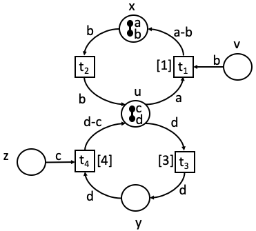
Figure 10: Causal execution where $\sigma=\langle t_{\_}1,t_{\_}2,t_{\_}3,t_{\_}4\rangle$

As a further example consider the example in Figure 10 demonstrating a cyclic RPN. Assume that $\sigma=\langle t_{\_}1,t_{\_}2,t_{\_}3,t_{\_}4\rangle$, i.e. from the initial state of the RPN the upper cycle is executed followed by the lower cycle. The transitions of the two cycles are causally independent since they manipulate different sets of tokens and therefore they can be reversed in any order. The figure illustrates the reversal of $t_{\_}2$ before $t_{\_}4$, which returns the bond between $a\!-\!b$ to place $x$.

In what follows we write $\stackrel{{\scriptstyle}}{{\longmapsto}}_{c}$ for $\stackrel{{\scriptstyle}}{{\longrightarrow}}\cup\stackrel{{\scriptstyle}}{{\rightsquigarrow}}_{c}$. The following result, similarly to Proposition 3, establishes that under the causal-order reversibility semantics, tokens are unique and preserved, bonds are unique, and they can only be created during forward execution and destroyed during reversal. Note that in what follows we will often omit the causal dependence relation and simply write $\langle{M},{H}\rangle$ for states when it is not relevant to the discussion.

Proposition 4.

Given a reversing Petri net $(A,P,B,T,F)$, an initial state $\langle M_{\_}0,H_{\_}0\rangle$ and an execution $\langle{M_{\_}0},{H_{\_}0}\rangle\stackrel{{\scriptstyle t_{\_}1}}{{\longmapsto}}_{c}\langle{M_{\_}1},{H_{\_}1}\rangle\stackrel{{\scriptstyle t_{\_}2}}{{\longmapsto}}_{c}\ldots\stackrel{{\scriptstyle t_{\_}n}}{{\longmapsto}}_{c}\langle{M_{\_}n},{H_{\_}n}\rangle$, the following hold:

1. For all $a\in A$ and $i$, $0\leq i\leq n$, $|\{x\in P\mid a\in M_{\_}i(x)\}|=1$.

2. For all $\beta\in B$ and $i$, $0\leq i\leq n$,

   1. $0\leq|\{x\in P\mid\beta\in M_{\_}i(x)\}|\leq 1$,

   2. if $t_{\_}i$ is executed in the forward direction and $\beta\in\mathsf{eff}(t_{\_}i)$, then $\beta\in M_{\_}{i}(x)$ for some $x\in P$ where $\beta\in F(t_{\_}i,x)$, and $\beta\not\in M_{\_}{i-1}(y)$ for all $y\in P$,

   3. if $t_{\_}i$ is executed in the forward direction, $\beta\in M_{\_}{i-1}(x)$ for some $x\in P$, and $\beta\not\in\mathsf{eff}(t_{\_}i)$, then, if $\beta\in\mathsf{con}(a,M_{\_}{i-1}(x))$ and $a\in F(t_{\_}i,y)$ then $\beta\in M_{\_}{i}(y)$, otherwise $\beta\in M_{\_}i(x)$

   4. if $t_{\_}i$ is executed in the reverse direction and $\beta\in\mathsf{eff}(t_{\_}i)$, then $\beta\in M_{\_}{i-1}(x)$ for some $x\in P$ where $\beta\in F(t_{\_}i,x)$, and $\beta\not\in M_{\_}{i}(y)$ for all $y\in P$, and

   5. if $t_{\_}i$ is executed in the reverse direction, $\beta\in M_{\_}{i-1}(x)$ for some $x\in P$, and $\beta\not\in\mathsf{eff}(t_{\_}i)$, then, if $\beta\in\mathsf{con}(a,M_{\_}{i-1}(x))$ and $a\in F(y,t_{\_}i)$ then $\beta\in M_{\_}{i}(y)$, otherwise $\beta\in M_{\_}i(x)$.

Proof:

The proof follows along the same lines as that of Proposition 3 with $\stackrel{{\scriptstyle}}{{\rightsquigarrow}}_{b}$ replaced by $\stackrel{{\scriptstyle}}{{\rightsquigarrow}}_{c}$. $\Box$

We may now establish the causal consistency of our semantics. First we define some auxiliary notions. Given a transition $\langle{M},{H}\rangle\stackrel{{\scriptstyle t}}{{\longmapsto}}_{c}\langle{M^{\prime}},{H^{\prime}}\rangle$, we say that the action of the transition is $t$ if $\langle{M},{H}\rangle\stackrel{{\scriptstyle t}}{{\longrightarrow}}\langle{M^{\prime}},{H^{\prime}}\rangle$ and $\underline{t}$ if $\langle{M},{H}\rangle\stackrel{{\scriptstyle t}}{{\rightsquigarrow}}_{c}\langle{M^{\prime}},{H^{\prime}}\rangle$ and we may write $\langle{M},{H}\rangle\stackrel{{\scriptstyle\underline{t}}}{{\longmapsto}}_{c}\langle{M^{\prime}},{H^{\prime}}\rangle$. We use $\alpha$ to range over $\{t,\underline{t}\mid t\in T\}$ and write $\underline{\underline{\alpha}}=\alpha$. We extend this notion to sequences of transitions and, given an execution $\langle{M_{\_}0},{H_{\_}0}\rangle\stackrel{{\scriptstyle t_{\_}1}}{{\longmapsto}}_{c}\ldots\stackrel{{\scriptstyle t_{\_}n}}{{\longmapsto}}_{c}\langle{M_{\_}n},{H_{\_}n}\rangle$, we say that the trace of the execution is $\sigma=\langle\alpha_{\_}1,\alpha_{\_}2,\ldots,\alpha_{\_}n\rangle$, where $\alpha_{\_}i$ is the action of transition $\langle{M_{\_}{i-1}},{H_{\_}{i-1}}\rangle\stackrel{{\scriptstyle t_{\_}i}}{{\longmapsto}}_{c}\langle{M_{\_}i},{H_{\_}i}\rangle$, and write $\langle{M},{H}\rangle\stackrel{{\scriptstyle\sigma}}{{\longmapsto}}_{c}\langle{M_{\_}n},{H_{\_}n}\rangle$. Given $\sigma_{\_}1=\langle\alpha_{\_}1,\ldots,\alpha_{\_}k\rangle$, $\sigma_{\_}2=\langle\alpha_{\_}{k+1},\ldots,\alpha_{\_}n\rangle$, we write $\sigma_{\_}1;\sigma_{\_}2$ for $\langle\alpha_{\_}1,\ldots,\alpha_{\_}n\rangle$. We may also use the notation $\sigma_{\_}1;\sigma_{\_}2$ when $\sigma_{\_}1$ or $\sigma_{\_}2$ is a single transition.

An execution of a Petri net can be partitioned as a set of independent flows of execution running through the net. We capture these flows by the notion of causal paths:

Definition 12.

Given a state $\langle{M},{H},{\prec}\rangle$ and transition occurrences $(t_{\_}i,k_{\_}i)$ in $\langle{M},{H},{\prec}\rangle$, $1\leq i\leq n$, we say that $(t_{\_}1,k_{\_}1),\ldots,(t_{\_}n,k_{\_}n)$ is a causal path in $\langle{M},{H},{\prec}\rangle$, if $(t_{\_}i,k_{\_}i)\prec(t_{\_}{i+1},k_{\_}{i+1})$, for all $0\leq i<n$.

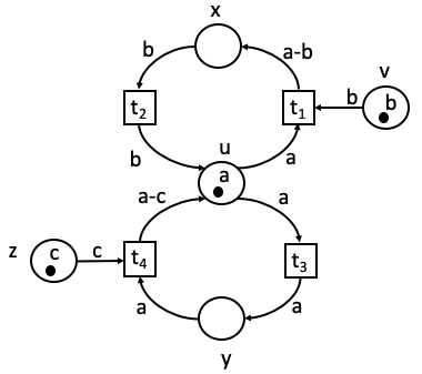
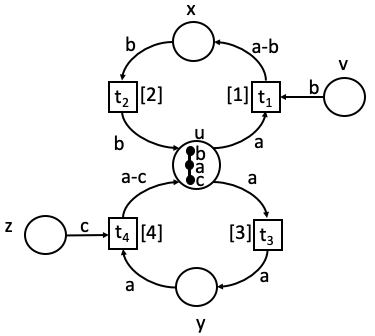
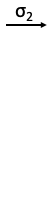
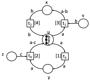
Figure 11: Causal paths in the context of independent cycles, where $\sigma_{\_}1=\langle t_{\_}1,t_{\_}2,t_{\_}3,t_{\_}4\rangle$ and $\sigma_{\_}2=\langle t_{\_}3,t_{\_}4,t_{\_}1,t_{\_}2\rangle$

As an example, consider the RPN in Figure 11 where we denote the first execution by $\langle{M_{\_}0},{H_{\_}0},{\emptyset}\rangle\stackrel{{\scriptstyle\sigma_{\_}1}}{{\longrightarrow}}\langle{M_{\_}4},{H_{\_}4},{\prec}\rangle$ for $\sigma_{\_}1=\langle t_{\_}1,t_{\_}2,t_{\_}3,t_{\_}4\rangle$, and the second execution by $\langle{M_{\_}0},{H_{\_}0},{\emptyset}\rangle\stackrel{{\scriptstyle\sigma_{\_}2}}{{\longrightarrow}}\langle{M_{\_}4^{\prime}},{H_{\_}4^{\prime}},{\prec^{\prime}}\rangle$ for $\sigma_{\_}2=\langle t_{\_}3,t_{\_}4,t_{\_}1,t_{\_}2\rangle$. In the case of $\sigma_{\_}1$ we have $\prec$ to be the transitive closure of $\{((t_{\_}1,1),(t_{\_}2,2)),$ $((t_{\_}2,2),(t_{\_}3,3)),((t_{\_}3,3),(t_{\_}4,4))\}$, which results in the causal path $(t_{\_}1,1),(t_{\_}2,2),$ $(t_{\_}3,3),(t_{\_}4,4)$. In the case of $\sigma_{\_}2$ where the cycles are executed in the opposite order, $\prec^{\prime}$ is the transitive closure of $\{((t_{\_}3,1),(t_{\_}4,2)),((t_{\_}4,2),(t_{\_}1,3)),((t_{\_}1,3),$ $(t_{\_}2,4))\}$, and the corresponding causal path is $(t_{\_}3,1),(t_{\_}4,2),(t_{\_}1,3),(t_{\_}2,4)$.

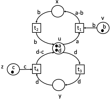
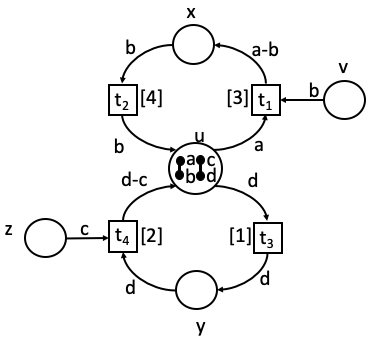
Figure 12: Causal paths in the context of independent cycles, where $\sigma_{\_}1=\langle t_{\_}1,t_{\_}2,t_{\_}3,t_{\_}4\rangle$ and $\sigma_{\_}2=\langle t_{\_}3,t_{\_}4,t_{\_}1,t_{\_}2\rangle$

This comes in contrast to the RPN of Figure 12, which contains two independent cycles. Here, the causal dependencies of the first execution (trace $\sigma_{\_}1$) are constructed as $(t_{\_}1,1)\prec(t_{\_}2,2)$ and $(t_{\_}3,3)\prec(t_{\_}4,4)$, which results in the two independent causal paths $\langle(t_{\_}1,1),(t_{\_}2,2)\rangle$ and $\langle(t_{\_}3,3),(t_{\_}4,4)\rangle$. Similarly, after execution of $\sigma_{\_}2$, the causal dependencies are $(t_{\_}1,3)\prec(t_{\_}2,4)$ and $(t_{\_}3,1)\prec(t_{\_}4,2)$, which results in the causal paths $\langle(t_{\_}1,3),(t_{\_}2,4)\rangle$ and $\langle(t_{\_}3,1),(t_{\_}4,2)\rangle$.

As seen from the examples in Figures 11 and 12, the causal paths of an execution capture its causal behavior. Based on this concept, we define the notion of causal equivalence for histories by requiring that two histories $H$ and $H^{\prime}$ are causally equivalent if and only if they contain the same causal paths:

Definition 13.

Consider a reversing Petri net $(A,P,B,T,F)$ and two executions $\langle{M},{H},{\prec}\rangle\stackrel{{\scriptstyle\sigma}}{{\longmapsto}}_{c}\langle{M^{\prime}},{H^{\prime}},{\prec^{\prime}}\rangle$ and $\langle{M},{H},{\prec}\rangle\stackrel{{\scriptstyle\sigma^{\prime}}}{{\longmapsto}}_{c}\langle{M^{\prime\prime}},{H^{\prime\prime}},{\prec^{\prime\prime}}\rangle$. Then the histories $H^{\prime}$ and $H^{\prime\prime}$ are causally equivalent, denoted by $H^{\prime}\asymp H^{\prime\prime}$, if for each causal path $(t_{\_}1,k_{\_}1),\ldots,(t_{\_}n,k_{\_}n)$ in $\langle{M^{\prime}},{H^{\prime}},{\prec^{\prime}}\rangle$, there is a causal path $(t_{\_}1,k_{\_}1^{\prime}),\ldots,(t_{\_}n,k_{\_}n^{\prime})$ in $\langle{M^{\prime\prime}},{H^{\prime\prime}},{\prec^{\prime\prime}}\rangle$, and vice versa.

We extend this notion and write $\langle{M},{H},{\prec}\rangle\asymp\langle{M^{\prime}},{H^{\prime}},{\prec^{\prime}}\rangle$ if and only if $M=M^{\prime}$ and $H\asymp H^{\prime}$.

Returning to the example in Figure 11 we observe that while the two executions result in the same marking, the resulting states do not have the same causal paths and, as such, they are not considered as causally equivalent.

We may now establish the Loop lemma.

Lemma 2 (Loop).

For any forward transition $\langle{M},{H}\rangle\stackrel{{\scriptstyle t}}{{\longrightarrow}}\langle{M^{\prime}},{H^{\prime}}\rangle$ there exists a backward transition $\langle{M^{\prime}},{H^{\prime}}\rangle\stackrel{{\scriptstyle t}}{{\rightsquigarrow}}_{c}\langle{M},{H}\rangle$ and for any backward transition $\langle{M},{H}\rangle\stackrel{{\scriptstyle t}}{{\rightsquigarrow}}_{c}\langle{M^{\prime}},{H^{\prime}}\rangle$ there exists a forward transition $\langle{M^{\prime}},{H^{\prime}}\rangle\stackrel{{\scriptstyle t}}{{\longrightarrow}}\langle{M},{H^{\prime\prime}}\rangle$ where $H\asymp H^{\prime\prime}$.

Proof:

The proof of the first direction follows along the same lines as that of Lemma 1 with $\stackrel{{\scriptstyle}}{{\rightsquigarrow}}_{b}$ replaced by $\stackrel{{\scriptstyle}}{{\rightsquigarrow}}_{c}$. For the other direction suppose $\langle{M},{H}\rangle\stackrel{{\scriptstyle t}}{{\rightsquigarrow}}_{c}\langle{M^{\prime}},{H^{\prime}}\rangle\stackrel{{\scriptstyle t}}{{\longrightarrow}}\langle{M},{H^{\prime\prime}}\rangle$. To begin with, we may observe that, as with Lemma 1, $M=M^{\prime\prime}$. To show that $H\asymp H^{\prime\prime}$, we observe that $H=H^{\prime\prime}$ with the exception of $t$, where, if $k=\max(H(t))$, and $k^{\prime}=\max(\{0\}\cup\{k^{\prime\prime}|(t^{\prime},k^{\prime\prime})\in H^{\prime}(t^{\prime}),t^{\prime}\in T\})+1$, then $H^{\prime\prime}(t)=(H(t)-\{k\})\cup\{k^{\prime}\})$. Furthermore, since $t$ is $co$-enabled in $\langle{M},{H}\rangle$, $(t,k)$ must be the last transition occurrence in all the causal paths it occurs in, and we may observe that $H^{\prime\prime}$ contains the same causal paths with $(t,k)$ replaced by $(t,k^{\prime})$. As a result it must be that $H\asymp H^{\prime\prime}$ and the result follows. $\Box$

We now proceed to define causal equivalence on traces, a notion that employs the concept of concurrent transitions:

Definition 14.

Actions $\alpha_{\_}1$ and $\alpha_{\_}2$ are concurrent in state $\langle{M},{H},{\prec}\rangle$, if whenever $\langle{M},{H},{\prec}\rangle\stackrel{{\scriptstyle\alpha_{\_}1}}{{\longmapsto}}_{c}\langle{M_{\_}1},{H_{\_}1},{\prec_{\_}1}\rangle$ and $\langle{M},{H},{\prec}\rangle\stackrel{{\scriptstyle\alpha_{\_}2}}{{\longmapsto}}_{c}\langle{M_{\_}2},{H_{\_}2},{\prec_{\_}2}\rangle$ then $\langle{M_{\_}1},{H_{\_}1},{\prec_{\_}1}\rangle\stackrel{{\scriptstyle\alpha_{\_}2}}{{\longmapsto}}_{c}\langle{M^{\prime}},{H^{\prime}},{\prec^{\prime}}\rangle$ and $\langle{M_{\_}2},{H_{\_}2},{\prec_{\_}2}\rangle\stackrel{{\scriptstyle\alpha_{\_}1}}{{\longmapsto}}_{c}$ $\langle{M^{\prime\prime}},{H^{\prime\prime}},{\prec^{\prime\prime}}\rangle$, where $\langle{M^{\prime}},{H^{\prime}},{\prec^{\prime}}\rangle\asymp\langle{M^{\prime\prime}},{H^{\prime\prime}},{\prec^{\prime\prime}}\rangle$.

Thus, two actions are concurrent if execution of the one does not preclude the other and the two execution orderings lead to causally equivalent states. The condition on final states being equivalent is required to rule out transitions constituting self-loops to/from the same place that are causally dependent on each other.

Definition 15.

Causal equivalence on traces, denoted by $\asymp$, is the least equivalence relation closed under composition of traces such that (i) if $\alpha_{\_}1$ and $\alpha_{\_}2$ are concurrent actions then $\alpha_{\_}1;\alpha_{\_}2\asymp\alpha_{\_}2;\alpha_{\_}1$ and (ii) $\alpha;\underline{\alpha}\asymp\epsilon$.

The first clause states that in two causally-equivalent traces concurrent actions may occur in any order and the second clause states that it is possible to ignore transitions that have occurred in both the forward and the reverse direction.

The following proposition establishes that two transition instances belonging to distinct causal paths are in fact concurrent transitions and thus can be executed in any order.

Proposition 5.

Consider a reversing Petri net $(A,P,B,T,F)$ and suppose $\langle M,H,{\prec}\rangle\stackrel{{\scriptstyle t_{\_}1}}{{\longrightarrow}}\langle{M_{\_}1},{H_{\_}1},{\prec_{\_}1}\rangle\stackrel{{\scriptstyle t_{\_}2}}{{\longrightarrow}}\langle{M_{\_}2},{H_{\_}2},{\prec_{\_}2}\rangle$, where the executions of $t_{\_}1$ and $t_{\_}2$ correspond to transition instances $(t_{\_}1,k_{\_}1)$ and $(t_{\_}2,k_{\_}2)$ in $\langle{M_{\_}2},{H_{\_}2},{\prec_{\_}2}\rangle$. If there is no causal path $\pi$ in $\langle{M_{\_}2},{H_{\_}2},{\prec_{\_}2}\rangle$ with $(t_{\_}1,k_{\_}1)\in\pi$ and $(t_{\_}2,k_{\_}2)\in\pi$, then $(t_{\_}1,k_{\_}1)$ and $(t_{\_}2,k_{\_}2)$ are concurrent transition occurrences in $\langle{M},{H},{\prec}\rangle$.

Proof:

Since there is no causal path containing both $(t_{\_}1,k_{\_}1)$ and $(t_{\_}2,k_{\_}2)$ in $\langle{M_{\_}2},{H_{\_}2},{\prec_{\_}2}\rangle$, we conclude that $(t_{\_}1,k_{\_}1)\not\prec_{\_}2(t_{\_}2,k_{\_}2)$. This implies that the two transition occurrences do not handle any common tokens and they can be executed in any order leading to the same marking. Thus, they are concurrent in $\langle{M},{H},{\prec}\rangle$. $\Box$

We note that causally-equivalent states can execute the same transitions.

Proposition 6.

Consider a reversing Petri net $(A,P,B,T,F)$ and states $\langle M,H_{\_}1,{\prec_{\_}1}\rangle\asymp\langle M,H_{\_}2,{\prec_{\_}2}\rangle$. Then $\langle{M},{H_{\_}1},{\prec_{\_}1}\rangle\stackrel{{\scriptstyle\alpha}}{{\longmapsto}}_{c}\langle{M_{\_}1},{H_{\_}1^{\prime}},{\prec_{\_}1^{\prime}}\rangle$ if and only if $\langle{M},{H_{\_}2},{\prec_{\_}2}\rangle\stackrel{{\scriptstyle\alpha}}{{\longmapsto}}_{c}\langle{M_{\_}2},{H_{\_}2^{\prime}},{\prec_{\_}2^{\prime}}\rangle$, where $\langle M_{\_}1,H_{\_}1^{\prime},{\prec_{\_}1^{\prime}}\rangle\asymp\langle M_{\_}2,H_{\_}2^{\prime},{\prec_{\_}2^{\prime}}\rangle$.

Proof:

It is easy to see that if a transition $\alpha$ is enabled in $\langle{M},{H_{\_}1},{\prec_{\_}1}\rangle$ it is also enabled in $\langle{M},{H_{\_}2},{\prec_{\_}2}\rangle$. Therefore, if $\langle{M},{H_{\_}1},{\prec_{\_}1}\rangle\stackrel{{\scriptstyle\alpha}}{{\longmapsto}}_{c}\langle{M_{\_}1},{H_{\_}1^{\prime}},{\prec_{\_}1^{\prime}}\rangle$ then $\langle{M},{H_{\_}2},{\prec_{\_}2}\rangle\stackrel{{\scriptstyle\alpha}}{{\longmapsto}}_{c}\langle{M_{\_}2},{H_{\_}2^{\prime}},{\prec_{\_}2^{\prime}}\rangle$ where $M_{\_}1=M_{\_}2$, and vice versa. In order to show that $H_{\_}1^{\prime}\asymp H_{\_}2^{\prime}$ two cases exist:

• Suppose $\alpha$ is a forward transition corresponding to transition occurrence $(t,k_{\_}1)$ in $\langle{M_{\_}1},{H_{\_}1^{\prime}},{\prec_{\_}1^{\prime}}\rangle$ and transition occurrence $(t,k_{\_}2)$ in $\langle;_{\_}2,H_{\_}2^{\prime},$ $\prec_{\_}2^{\prime}\rangle$. Suppose that $(t^{\prime},k_{\_}1^{\prime})\prec_{\_}1^{\prime}(t,k_{\_}1)$. Then, $\mathsf{post}(t^{\prime})\cap\mathsf{con}(a,M(x))\neq\emptyset$ for some $a\in F(x,t)$. Since $H_{\_}1\asymp H_{\_}2$, this implies that $(t^{\prime},k_{\_}2^{\prime})\prec_{\_}2^{\prime}(t,k_{\_}2)$ where $k_{\_}2^{\prime}=\max(H_{\_}2(t^{\prime}))$. since $H_{\_}1\asymp H_{\_}2$.) Therefore, for all causal paths $\pi$ in $\langle{M},{H_{\_}1},{\prec_{\_}1}\rangle$, if the last transition occurrence of $\pi$ causes $(t,k_{\_}1)$ then $\pi;(t,k_{\_}1)$ is a causal path of $\langle{M_{\_}1},{H_{\_}1^{\prime}},{\prec_{\_}1^{\prime}}\rangle$ and, if not, then $\pi$ is a causal path in $\langle{M_{\_}1},{H_{\_}1^{\prime}},{\prec_{\_}1^{\prime}}\rangle$. The same holds for causal paths in $\langle{M_{\_}2},{H_{\_}2^{\prime}},{\prec_{\_}2^{\prime}}\rangle$ and $(t,k_{\_}2)$. Consequently, we deduce that $H_{\_}1^{\prime}\asymp H_{\_}2^{\prime}$, as required.

• Suppose that $\alpha$ is a reverse transition, i.e. $\alpha=\underline{t}$ for some $t$, and consider the causal paths of $H_{\_}1^{\prime}$ and $H_{\_}2^{\prime}$. Since $\alpha$ is a reverse transition, there exists no transition occurrence caused by $(t,\max(H_{\_}1(t)))$ in $\langle{M},{H_{\_}1},{\prec_{\_}1}\rangle$ and no transition occurrence caused by $(t,\max(H_{\_}2(t)))$ in $\langle{M},{H_{\_}2},{\prec_{\_}2}\rangle$. As such, $(t,\max(H_{\_}1(t)))$ and $(t,\max(H_{\_}2(t)))$ are the last transition occurrences in all paths in $\langle{M},{H_{\_}1},{\prec_{\_}1}\rangle$ and $\langle{M},{H_{\_}2},{\prec_{\_}2}\rangle$, respectively, in which they belong. Reversing the transition occurrences results in their elimination from these causal paths. Therefore, we observe that for each causal path in $\langle{M_{\_}1},{H_{\_}1^{\prime}},{\prec_{\_}1^{\prime}}\rangle$ there is an equivalent causal path in $\langle{M_{\_}2},{H_{\_}2^{\prime}},{\prec_{\_}2^{\prime}}\rangle$, and vice versa. Thus $H_{\_}1^{\prime}\asymp H_{\_}2^{\prime}$ as required. $\Box$

Note that the above result can be extended to sequences of transitions:

Corollary 1.

Consider a reversing Petri net $(A,P,B,T,F)$ and states $\langle M,$ $H_{\_}1,{\prec_{\_}1}\rangle\asymp\langle M,H_{\_}2,{\prec_{\_}2}\rangle$. Then $\langle{M},{H_{\_}1},{\prec_{\_}1}\rangle\stackrel{{\scriptstyle\sigma}}{{\longmapsto}}_{c}\langle{M_{\_}1},{H_{\_}1^{\prime}},{\prec_{\_}1^{\prime}}\rangle$ if and only if $\langle{M},{H_{\_}2},{\prec_{\_}2}\rangle\stackrel{{\scriptstyle\sigma}}{{\longmapsto}}_{c}\langle{M_{\_}2},{H_{\_}2^{\prime}},{\prec_{\_}2^{\prime}}\rangle$, where $\langle M_{\_}1,H_{\_}1^{\prime},{\prec_{\_}1^{\prime}}\rangle\asymp\langle M_{\_}2,H_{\_}2^{\prime},{\prec_{\_}2^{\prime}}\rangle$.

The main result, Theorem 1 below, states that two computations beginning in the same initial state lead to equivalent states if and only if the sequences of executed transitions of the two computations are causally equivalent. This guarantees the consistency of the approach since reversing transitions in causal order is in a sense equivalent to not executing the transitions in the first place. Reversal does not give rise to previously unreachable states, on the contrary, it gives rise to exactly the same markings and causally-equivalent histories due to the different keys being possibly assigned because of the different ordering of transitions.

Theorem 1.

Consider executions $\langle{M},{H}\rangle\stackrel{{\scriptstyle\sigma_{\_}1}}{{\longmapsto}}_{c}\langle{M_{\_}1},{H_{\_}1}\rangle$ and $\langle{M},{H}\rangle\stackrel{{\scriptstyle\sigma_{\_}2}}{{\longmapsto}}_{c}\langle{M_{\_}2},{H_{\_}2}\rangle$. Then, $\sigma_{\_}1\asymp\sigma_{\_}2$ if and only if $\langle{M_{\_}1},{H_{\_}1}\rangle\asymp\langle{M_{\_}2},{H_{\_}2}\rangle$.

For the proof of Theorem 1 we employ some intermediate results. To begin with, the lemma below states that causal equivalence allows the permutation of reverse and forward transitions that have no causal relations between them. Therefore, computations are allowed to reach for the maximum freedom of choice going backward and then continue forward.

Lemma 3.

Let $\sigma$ be a trace. Then there exist traces $r,r^{\prime}$ both forward such that $\sigma\asymp\underline{r};r^{\prime}$ and if $\langle{M},{H}\rangle\stackrel{{\scriptstyle\sigma}}{{\longmapsto}}\langle{M^{\prime}},{H^{\prime}}\rangle$ then $\langle{M},{H}\rangle\stackrel{{\scriptstyle\underline{r};r^{\prime}}}{{\longmapsto}}\langle{M^{\prime}},{H^{\prime\prime}}\rangle$, where $H^{\prime}\asymp H^{\prime\prime}$.

Proof:

We prove this by induction on the length of $\sigma$ and the distance from the beginning of $\sigma$ to the earliest pair of transitions that contradicts the property $\underline{r};r^{\prime}$. If there is no such contradicting pair then the property is trivially satisfied. If not, we distinguish the following cases:

1. If the first contradicting pair is of the form $t;\underline{t}$ then we have $\langle{M},{H}\rangle\stackrel{{\scriptstyle\sigma_{\_}1}}{{\longmapsto}}_{c}\langle{M_{\_}1},{H_{\_}1}\rangle\stackrel{{\scriptstyle t}}{{\longmapsto}}_{c}\langle{M_{\_}2},{H_{\_}2}\rangle\stackrel{{\scriptstyle\underline{t}}}{{\longmapsto}}_{c}\langle{M_{\_}3},{H_{\_}3}\rangle\stackrel{{\scriptstyle\sigma_{\_}2}}{{\longmapsto}}_{c}\langle{M^{\prime}},{H^{\prime}}\rangle$ where $\sigma=\sigma_{\_}1;t;\underline{t};\sigma_{\_}2$. By the Loop Lemma $\langle{M_{\_}1},{H_{\_}1}\rangle=\langle{M_{\_}3},{H_{\_}3}\rangle$, which yields $\langle{M},{H}\rangle\stackrel{{\scriptstyle\sigma_{\_}1}}{{\longmapsto}}_{c}\langle{M_{\_}1},{H_{\_}1}\rangle\stackrel{{\scriptstyle\sigma_{\_}2}}{{\longmapsto}}_{c}\langle{M^{\prime}},{H^{\prime}}\rangle$. Thus we may remove the two transitions from the sequence, the length of $\sigma$ decreases, and the proof follows by induction.

2. If the first contradicting pair is of the form $t;\underline{t}^{\prime}$ then we observe that the specific occurrences of $t$ and $\underline{t}^{\prime}$ must be concurrent. Specifically we have $\langle{M},{H}\rangle\stackrel{{\scriptstyle\sigma_{\_}1}}{{\longmapsto}}_{c}\langle{M_{\_}1},{H_{\_}1}\rangle\stackrel{{\scriptstyle t}}{{\longmapsto}}_{c}\langle{M_{\_}2},{H_{\_}2}\rangle\stackrel{{\scriptstyle\underline{t^{\prime}}}}{{\longmapsto}}_{c}\langle{M_{\_}3},{H_{\_}3}\rangle\stackrel{{\scriptstyle\sigma_{\_}2}}{{\longmapsto}}_{c}\langle{M^{\prime}},{H^{\prime}}\rangle$ where $\sigma=\sigma_{\_}1;t;\underline{t^{\prime}};\sigma_{\_}2$. Since action $t^{\prime}$ is being reversed, all transition occurrences that are causally dependent on it have either not been executed up to this point or they have already been reversed. This implies that in $\langle{M_{\_}2},{H_{\_}2}\rangle$ it was not the case that $(t^{\prime},max(H_{\_}2(t^{\prime}))$ was causally dependent on $(t,max(H_{\_}2(t))$. As such, by Proposition 5, $\underline{t^{\prime}}$ and $t$ are concurrent transitions and $t^{\prime}$ can be reversed before the execution of $t$ to yield $\langle{M},{H}\rangle\stackrel{{\scriptstyle\sigma_{\_}1}}{{\longmapsto}}_{c}\langle{M_{\_}1},{H_{\_}1}\rangle\stackrel{{\scriptstyle\underline{t^{\prime}}}}{{\longmapsto}}_{c}\langle{M_{\_}2^{\prime}},{H_{\_}2^{\prime}}\rangle\stackrel{{\scriptstyle t}}{{\longmapsto}}_{c}\langle{M_{\_}3},{H_{\_}3^{\prime}}\rangle\stackrel{{\scriptstyle\sigma_{\_}2}}{{\longmapsto}}_{c}\langle{M^{\prime}},{H^{\prime\prime}}\rangle$, where $H_{\_}3^{\prime}\asymp H_{\_}3$ and $H^{\prime}\asymp H^{\prime\prime}$. This results in a later earliest contradicting pair and by induction the result follows. $\Box$

From the above lemma we conclude the following corollary establishing that causal-order reversibility is consistent with standard forward execution in the sense that causal execution will not generate states that are unreachable in forward execution:

Corollary 2.

Suppose that $H_{\_}0$ is the initial history. If $\langle{M_{\_}0},{H_{\_}0}\rangle\stackrel{{\scriptstyle\sigma}}{{\longmapsto}}_{c}\langle{M},{H}\rangle$, and $\sigma$ is a trace with both forward and backward transitions then there exists a transition $\langle{M_{\_}0},{H_{\_}0}\rangle\stackrel{{\scriptstyle\sigma^{\prime}}}{{\longmapsto}}_{c}\langle{M},{H^{\prime}}\rangle$, where $H\asymp H^{\prime}$ and $\sigma^{\prime}$ a trace of forward transitions.

Proof:

According to Lemma 3, $\sigma\asymp\underline{r};r^{\prime}$ where both $r$ and $r^{\prime}$ are forward traces. Since, however, $H_{\_}0$ is the initial history it must be that $r$ is empty. This implies that $\langle{M_{\_}0},{H_{\_}0}\rangle\stackrel{{\scriptstyle r^{\prime}}}{{\longmapsto}}_{c}\langle{M},{H^{\prime}}\rangle$, $H\asymp H^{\prime}$ and $r^{\prime}$ is a forward trace. Consequently, writing $\sigma^{\prime}$ for $r^{\prime}$, the result follows. $\Box$

Lemma 4.

Suppose $\langle{M},{H}\rangle\stackrel{{\scriptstyle\sigma_{\_}1}}{{\longmapsto}}_{c}\langle{M^{\prime}},{H_{\_}1}\rangle$ and $\langle{M},{H}\rangle\stackrel{{\scriptstyle\sigma_{\_}2}}{{\longmapsto}}_{c}\langle{M^{\prime}},{H_{\_}2}\rangle$, where $H_{\_}1\asymp H_{\_}2$ and $\sigma_{\_}2$ is a forward trace. Then, there exists a forward trace $\sigma_{\_}1^{\prime}$ such that $\sigma_{\_}1\asymp\sigma_{\_}1^{\prime}$.

Proof:

If $\sigma_{\_}1$ is forward then $\sigma_{\_}1=\sigma_{\_}1^{\prime}$ and the result follows trivially. Otherwise, we may prove the lemma by induction on the length of $\sigma_{\_}1$. We begin by noting that, by Lemma 3, $\sigma_{\_}1\asymp\underline{r};r^{\prime}$ and $\langle{M},{H}\rangle\stackrel{{\scriptstyle\underline{r};r^{\prime}}}{{\longmapsto}}_{c}\langle{M^{\prime}},{H_{\_}1}\rangle$. Let $\underline{t}$ be the last action in $\underline{r}$. Given that $\sigma_{\_}2$ is a forward execution that simulates $\sigma_{\_}1$, it must be that $r^{\prime}$ contains a forward execution of transition $t$ so that $\langle{M^{\prime}},{H_{\_}1}\rangle$ and $\langle{M^{\prime}},{H_{\_}2}\rangle$ contain the same causal paths involving transition $t$ (if not we would have $|H_{\_}1(t)|<|H_{\_}2(t)|$ leading to a contradiction). Consider the earliest occurrence of $t$ in $r^{\prime}$. If $t$ is the first transition in $r^{\prime}$, by the Loop Lemma we may remove the pair of opposite transitions and the result follows by induction. Otherwise, suppose $\langle{M},{H}\rangle\stackrel{{\scriptstyle\underline{r_{\_}1}}}{{\longmapsto}}_{c}\stackrel{{\scriptstyle\underline{t}}}{{\longmapsto}}_{c}\stackrel{{\scriptstyle{r_{\_}1^{\prime}}}}{{\longmapsto}}_{c}\langle{M_{\_}1},{H_{\_}3}\rangle\stackrel{{\scriptstyle t*}}{{\longmapsto}}_{c}\stackrel{{\scriptstyle t}}{{\longmapsto}}_{c}\langle{M_{\_}1^{\prime}},{H_{\_}4}\rangle\stackrel{{\scriptstyle r_{\_}2^{\prime}}}{{\longmapsto}}_{c}\langle{M^{\prime}},{H_{\_}1}\rangle$, where $r=r_{\_}1;t$ and $r^{\prime}=r_{\_}1^{\prime};t*;t;r_{\_}2$. Two cases exist:

1. Suppose $t*\in\sigma_{\_}2$. Let us denote by $num(t,\sigma)$, the number of executions of transition $t$ in a sequence of transitions $\sigma$. We observe that since $\sigma_{\_}2$ contains no reverse executions of $t$, it must be that $num(t,r^{\prime})=num(t,\sigma_{\_}2)+num(t,r)$. Suppose that the transition occurrences of $t*$ and $t$ as shown in the execution belong to a common causal path. We may extend this path with the succeeding occurrences of $t$ and obtain a causal path such that $t*$ is succeeded by $num(t,\sigma_{\_}2)+num(t,r)$ occurrences of $t$. We observe that it is impossible to obtain such a causal path in $\langle{M^{\prime}},{H_{\_}2}\rangle$, since $t*$ is followed by fewer occurrences of $t$ in $\sigma_{\_}2$. This contradicts the assumption that $H_{\_}1\asymp H_{\_}2$. We conclude that the transition occurrences of $t$ and $t*$ above do not belong to any common causal path and therefore, by Proposition 5, the two transition occurrences are concurrent in $\langle{M_{\_}1},{H_{\_}3}\rangle$.

2. Now suppose that $t*\not\in\sigma_{\_}2$. Since $H_{\_}1(t*)\neq\emptyset$ it must be that $H_{\_}2(t*)\neq\emptyset$ and $|H(t*)|=|H_{\_}1(t*)|=|H_{\_}2(t*)|$. As such, it must be that $t*\in r$ and that its reversal has preceded the reversal of $t$. Let us suppose that the transition occurrences of $t*$ and $t$ as shown in the execution belong to a common causal path. This implies that a causal path with $t*$ preceding $t$ also occurs in $H_{\_}2$ as well as in $H$. If we observe that $t*$ has reversed before $t$ we conclude that $t*$ does not cause the preceding occurrence of $t$. As such there is no causal path within $\langle{M},{H}\rangle$ or $\langle{M^{\prime}},{H_{\_}2}\rangle$ containing both $t$ and $t*$, which results in a contradiction. We conclude that the forward occurrences of $t$ and $t*$ are, by Proposition 5, concurrent in $\langle{M_{\_}1},{H_{\_}3}\rangle$.

Given the above, since the occurrences of $t$ and $t*$ are concurrent the two occurrences may be swapped to yield $\langle{M},{H}\rangle\stackrel{{\scriptstyle\underline{r_{\_}1}}}{{\longmapsto}}_{c}\stackrel{{\scriptstyle\underline{t}}}{{\longmapsto}}_{c}\stackrel{{\scriptstyle{r_{\_}1^{\prime}}}}{{\longmapsto}}_{c}\langle{M_{\_}1},{H_{\_}3}\rangle\stackrel{{\scriptstyle t}}{{\longmapsto}}_{c}\stackrel{{\scriptstyle t*}}{{\longmapsto}}_{c}\langle{M_{\_}1^{\prime}},{H_{\_}4^{\prime}}\rangle\stackrel{{\scriptstyle r_{\_}2^{\prime}}}{{\longmapsto}}_{c}\langle{M^{\prime}},{H_{\_}1^{\prime}}\rangle$ where $H_{\_}4\asymp H_{\_}4^{\prime}$ and, by Corollary 1, $H_{\_}1\asymp H_{\_}1^{\prime}$. By repeating the process for the remaining transition occurrences in $r_{\_}1^{\prime}$, this implies that we may permute $t$ with transitions in $r_{\_}1^{\prime}$ to yield the sequence $\underline{t};t$. By the Loop Lemma we may remove the pair of opposite transitions and obtain a shorter equivalent trace, also equivalent to $\sigma_{\_}2$ and conclude by induction. $\Box$

We now proceed with the proof of Theorem 1:

Proof of Theorem 1:

Suppose $\langle{M},{H}\rangle\stackrel{{\scriptstyle\sigma_{\_}1}}{{\longmapsto}}_{c}\langle{M_{\_}1},{H_{\_}1}\rangle$, $\langle{M},{H}\rangle\stackrel{{\scriptstyle\sigma_{\_}2}}{{\longmapsto}}_{c}\langle{M_{\_}2},{H_{\_}2}\rangle$ with $\langle{M_{\_}1},{H_{\_}1}\rangle\asymp\langle{M_{\_}2},{H_{\_}2}\rangle$. We prove that $\sigma_{\_}1\asymp\sigma_{\_}2$ by using a lexicographic induction on the pair consisting of the sum of the lengths of $\sigma_{\_}1$ and $\sigma_{\_}2$ and the depth of the earliest disagreement between them. By Lemma 3 we may suppose that $\sigma_{\_}1$ and $\sigma_{\_}2$ satisfy the property $\underline{r};r^{\prime}$. Call $t_{\_}1$ and $t_{\_}2$ the earliest actions where they disagree. There are three cases in the argument depending on whether these are forward or backward.

1. If $t_{\_}1$ is backward and $t_{\_}2$ is forward, we have $\sigma_{\_}1=\underline{r};\underline{t_{\_}1};u$ and $\sigma_{\_}2=\underline{r};t_{\_}2;v$ for some $r,u,v$. Lemma 4 applies to $t_{\_}2;v$, which is forward, and $\underline{t_{\_}1};u$, which contains both forward and backward actions and thus, by the lemma, it has a shorter forward equivalent. Thus, $\sigma_{\_}1$ has a shorter forward equivalent and the result follows by induction.

2. If $t_{\_}1$ and $t_{\_}2$ are both forward then it must be the case that $\sigma_{\_}1={\underline{r};r^{\prime}};t_{\_}1;u$ and $\sigma_{\_}2={\underline{r};r^{\prime}};t_{\_}2;v$, for some $r$, $u$, $v$. Note that it must be that $t_{\_}1\in v$ and $t_{\_}2\in u$. If not, we would have $|H_{\_}1(t_{\_}1)|\neq|H_{\_}2(t_{\_}1)|$, and similarly for $t_{\_}2$, which contradicts the assumption that ${H_{\_}1}\asymp{H_{\_}2}$. As such, we may write $\sigma_{\_}1={\underline{r};r^{\prime}};t_{\_}1;u_{\_}1;t_{\_}2;u_{\_}2$, where $u=u_{\_}1;t_{\_}2;u_{\_}2$ and $t_{\_}2$ is the first occurrence of $t_{\_}2$ in $u$. Consider $t*$ the action immediately preceding $t_{\_}2$. We observe that $t*$ and $t_{\_}2$ cannot belong to a common causal path in $\langle{M_{\_}1},{H_{\_}1}\rangle$, since an equivalent causal path is impossible to exist in $\langle{M_{\_}2},{H_{\_}2}\rangle$. This is due to the assumption that $\sigma_{\_}1$ and $\sigma_{\_}2$ coincide up to transition sequence $\underline{r};r^{\prime}$. Thus, we conclude by Proposition 5 that $t*$ and $t_{\_}2$ are in fact concurrent and can be swapped. The same reasoning may be used for all transitions preceding $t_{\_}2$ up to and including $t_{\_}1$, which leads to the conclusion that $\sigma_{\_}1\asymp{\underline{r};r^{\prime}};t_{\_}2;t_{\_}1;u_{\_}1;u_{\_}2$. This results in an equivalent execution of the same length with a later earliest divergence with $\sigma_{\_}2$ and the result follows by the induction hypothesis.

3. If $t_{\_}1$ and $t_{\_}2$ are both backward, we have $\sigma_{\_}1=\underline{r};\underline{t_{\_}1};u$ and $\sigma_{\_}2=\underline{r};\underline{t_{\_}2};v$ for some $r,u,v$. Two cases exist:

   1. If $\underline{t_{\_}1}$ occurs in $v$, then we have that $\sigma_{\_}2=\underline{r};\underline{t_{\_}2};\underline{v_{\_}1};\underline{t_{\_}1};v_{\_}2$. Given that $t_{\_}1$ reverses right after $\underline{r}$ in $\sigma_{\_}1$, we may conclude that there is no transition occurrence at this point that causally depends on $t_{\_}1$. As such it cannot have caused the transition occurrences of $t_{\_}2$ and ${v_{\_}1}$ whose reversal precedes it in $\sigma_{\_}2$. This implies that the reversal of $t_{\_}1$ may be swapped in $\sigma_{\_}2$ with each of the preceding transitions, to give $\sigma_{\_}2\asymp\underline{r};\underline{t_{\_}1};\underline{t_{\_}2};\underline{v_{\_}1};v_{\_}2$. This results in an equivalent execution of the same length with a later earliest divergence with $\sigma_{\_}1$ and the result follows by the induction hypothesis.

   2. If $\underline{t_{\_}1}$ does not occur in $v$, this implies that $t_{\_}1$ occurs in the forward direction in $u$, i.e. $\sigma_{\_}1=\underline{r};\underline{t_{\_}1};u_{\_}1;t_{\_}1;u_{\_}2$, where $u=u_{\_}1;t_{\_}1;u_{\_}2$ with the specific occurrence of $t_{\_}1$ being the first such occurrence in $u$. Using similar arguments as those in Lemma 4, we conclude that $\sigma_{\_}1\asymp\underline{r};\underline{t_{\_}1};t_{\_}1;u_{\_}1;u_{\_}2\asymp\underline{r};u_{\_}1;u_{\_}2$, an equivalent execution of shorter length for $\sigma_{\_}1$ and the result follows by the induction hypothesis.

   We may now prove the opposite direction. Suppose that $\sigma_{\_}1\asymp\sigma_{\_}2$ and $\langle{M},{H}\rangle\stackrel{{\scriptstyle\sigma_{\_}1}}{{\longmapsto}}_{c}\langle{M_{\_}1},{H_{\_}1}\rangle$ and $\langle{M},{H}\rangle\stackrel{{\scriptstyle\sigma_{\_}2}}{{\longmapsto}}_{c}\langle{M_{\_}2},{H_{\_}2}\rangle$. We will show that $\langle{M_{\_}1},{H_{\_}1}\rangle\asymp\langle{M_{\_}2},{H_{\_}2}\rangle$. The proof is by induction on the number of rules, $k$, applied to establish the equivalence $\sigma_{\_}1\asymp\sigma_{\_}2$. For the base case we have $k=0$, which implies that $\sigma_{\_}1=\sigma_{\_}2$ and the result trivially follows. For the inductive step, let us assume that $\sigma_{\_}1\asymp\sigma_{\_}1^{\prime}\asymp\sigma_{\_}2$, where $\sigma_{\_}1$ can be transformed to $\sigma_{\_}1^{\prime}$ with the use of $k=n-1$ rules and $\sigma_{\_}1^{\prime}$ can be transformed to $\sigma_{\_}2$ with the use of a single rule. By the induction hypothesis, we conclude that $\langle{M},{H}\rangle\stackrel{{\scriptstyle\sigma_{\_}1^{\prime}}}{{\longmapsto}}_{c}\langle{M_{\_}1},{H_{\_}1^{\prime}}\rangle$, where $H_{\_}1\asymp H_{\_}1^{\prime}$. We need to show that $\langle{M_{\_}1},{H_{\_}1^{\prime}}\rangle\asymp\langle{M_{\_}2},{H_{\_}2}\rangle$. Let us write $\sigma_{\_}1^{\prime}=u;w;v$ and $\sigma_{\_}2=u;w^{\prime};v$, where $w$, $w^{\prime}$ refer to the parts of the two executions where the equivalence rule has been applied. Furthermore, suppose that $\langle{M},{H}\rangle\stackrel{{\scriptstyle u}}{{\longmapsto}}_{c}\langle{M_{\_}u},{H_{\_}u}\rangle\stackrel{{\scriptstyle w}}{{\longmapsto}}_{c}\langle{M_{\_}w},{H_{\_}w}\rangle\stackrel{{\scriptstyle v}}{{\longmapsto}}_{c}\langle{M_{\_}1},{H_{\_}1^{\prime}}\rangle$ and $\langle{M},{H}\rangle\stackrel{{\scriptstyle u}}{{\longmapsto}}_{c}\langle{M_{\_}u},{H_{\_}u}\rangle\stackrel{{\scriptstyle w^{\prime}}}{{\longmapsto}}_{c}\langle{M_{\_}w^{\prime}},{H_{\_}w^{\prime}}\rangle\stackrel{{\scriptstyle v}}{{\longmapsto}}_{c}\langle{M_{\_}2},{H_{\_}2}\rangle$. Three cases exist:

   1. $w=t_{\_}1;t_{\_}2$ and $w^{\prime}=t_{\_}2;t_{\_}1$ with $t_{\_}1$ and $t_{\_}2$ concurrent

   2. $w=t;\underline{t}$ and $w^{\prime}=\epsilon$

   3. $w=\underline{t};t$ and $w^{\prime}=\epsilon$

   In all the cases above, we have that $\langle{M_{\_}w},{H_{\_}w}\rangle\asymp\langle{M_{\_}w^{\prime}},{H_{\_}w^{\prime}}\rangle$: for (a) this follows by the definition of concurrent transitions, whereas for (b) and (c) by the Loop Lemma. Given the equivalence of these two states, by Corollary 2, we have that $\langle{M_{\_}w},{H_{\_}w}\rangle\stackrel{{\scriptstyle v}}{{\longmapsto}}_{c}\langle{M_{\_}1},{H_{\_}1^{\prime}}\rangle$ and $\langle{M_{\_}w^{\prime}},{H_{\_}w^{\prime}}\rangle\stackrel{{\scriptstyle v}}{{\longmapsto}}_{c}\langle{M_{\_}2},{H_{\_}2}\rangle$, where $\langle{M_{\_}1},{H_{\_}1^{\prime}}\rangle\asymp\langle{M_{\_}2},{H_{\_}2}\rangle$, as required. This completes the proof. $\Box$

5.3 Out-of-causal-order reversibility

While in backtracking and causal-order reversibility reversing is cause respecting, there are many examples of systems where undoing actions in an out-of-causal order is either inherent or desirable. In this section we consider this type of reversibility in the context of RPNs. We begin by specifying that in out-of-causal-order reversibility any executed transition can be reversed at any time.

Definition 16.

Consider a reversing Petri net $(A,P,B,T,F)$, a state $\langle{M},{H}\rangle$, and a transition $t\in T$. We say that $t$ is $o$-enabled in $\langle{M},{H}\rangle$, if $H(t)\neq\emptyset$.

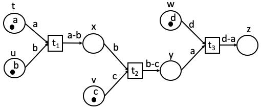
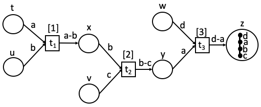
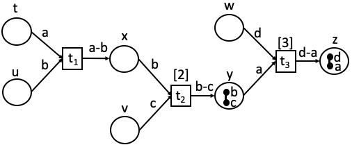
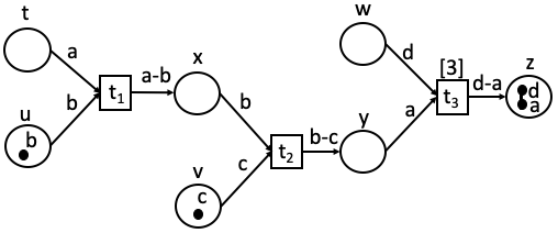
Figure 13: Out-of-causal-order example

Let us begin to consider out-of-causal-order reversibility via the example of Figure 13. The first two nets in the figure present the forward execution of the transition sequence $\langle t_{\_}1,t_{\_}2,t_{\_}3\rangle$. Suppose that transition $t_{\_}1$ is to be reversed out of order. The effect of this reversal should be the destruction of the bond between $a$ and $b$. This means that the component $d\!-\!a\!-\!b\!-\!c$ is broken into the bonds $d\!-\!a$ and $b\!-\!c$, which should backtrack within the net to capture the reversal of the transition. Nonetheless, the tokens of $d\!-\!a$ must remain at place $z$. This is because a bond exists between them that has not been reversed and was the effect of the immediately preceding transition $t_{\_}3$. However, in the case of $b\!-\!c$, the bond can be returned to place $y$, which is the place where the two tokens were connected and from where they could continue to participate in any further computation requiring their coalition. Once transition $t_{\_}2$ is subsequently reversed, the bond between $b$ and $c$ is destroyed and thus the two tokens are able to return to their initial places as shown in the third net in the figure. Finally, when subsequently transition $t_{\_}3$ is reversed, the bond between $d$ and $a$ breaks and, given that neither $d$ nor $a$ are connected to other elements, the tokens return to their initial places. As with the other types of reversibility, when reversing a transition histories are updated by removing the greatest key identifier of the executed transition.

Summing up, the effect of reversing a transition in out-of-causal order is that all bonds created by the transition are undone. This may result in tokens backtracking in the net. Further, if the reversal of a transition causes a coalition of bonds to be broken down into a set of subcomponents due to the destruction of bonds, then each of these coalitions should flow back, as far back as possible, after the last transition in which this sub-coalition participated. To capture this notion of “as far backwards as possible” we introduce the following:

Definition 17.

Given a reversing Petri net $(A,P,B,T,F)$, an initial marking $M_{\_}0$, a history $H$, and a set of bases and bonds $C\subseteq A\cup B$ we write:

$$\begin{array}[]{rcl}\mathsf{last}_{T}(C,H)&=&\left\{\begin{array}[]{ll}t,\;\;\textrm{ if }\exists t,\;\mathsf{post}(t)\cap C\neq\emptyset,\;H(t)\neq\emptyset,\mbox{ and }\\ \hskip 18.06749pt\not\exists t^{\prime},\;\mathsf{post}(t^{\prime})\cap C\neq\emptyset,\;H(t^{\prime})\neq\emptyset\;,\\ \hskip 18.06749ptmax(H(t^{\prime}))\geq max(H(t))\\ \bot,\;\textrm{ otherwise }\end{array}\right.\end{array}$$

$$\begin{array}[]{rcl}\mathsf{last}_{P}(C,H)&=&\left\{\begin{array}[]{ll}x,\;\;\textrm{ if }t=\mathsf{last}_{T}(C,H),\{x\}=\{y\in t\circ\mid F(t,y)\cap C\neq\emptyset\}\\ \hskip 18.06749pt\textrm{or, if }\bot=\mathsf{last}_{T}(C,H),C\subseteq M_{\_}0(x)\\ \bot,\;\textrm{ otherwise }\end{array}\right.\end{array}$$

Thus, if component $C$ has been manipulated by some previously-executed transition, then $\mathsf{last}_{T}(C,H)$ is the last executed such transition. Otherwise, if no such transition exists (e.g., because all transitions involving $C$ have been reversed), then $\mathsf{last}_{T}(C,H)$ is undefined ($\bot$). Similarly, $\mathsf{last}_{P}(C,H)$ is the outgoing place connected to $\mathsf{last}_{T}(C,H)\neq\bot$ having common tokens with $C$, assuming that such a place is unique, or the place in the initial marking in which $C$ existed if $\mathsf{last}_{T}(C,H)=\bot$, and undefined otherwise.

Transition reversal in an out-of-causal order can thus be defined as follows:

Definition 18.

Given a reversing Petri net $(A,P,B,T,F)$, an initial marking $M_{\_}0$, a state $\langle M,H\rangle$ and a transition $t$ that is $o$-enabled in $\langle{M},{H}\rangle$, we write $\langle{M},{H}\rangle\stackrel{{\scriptstyle t}}{{\rightsquigarrow}}_{o}\langle{M^{\prime}},{H^{\prime}}\rangle$ where $H^{\prime}$ is defined as in Definition 6 and we have:

$$M^{\prime}(x) = \Big{(}M(x)\cup\bigcup_{\_}{a\in M(y){\cap\mathsf{post}(t)},\mathsf{last}_{P}(C_{\_}{a,y},H^{\prime})=x}C_{\_}{a,y}\Big{)}$$

$$-\Big{(}\mathsf{eff}(t)\cup\bigcup_{\_}{a\in M(x){\cap\mathsf{post}(t)},\mathsf{last}_{P}(C_{\_}{a,x},H^{\prime})\neq x}C_{\_}{a,x}\Big{)}$$

where we use the shorthand $C_{\_}{b,z}=\mathsf{con}(b,M(z)-\mathsf{eff}(t))$ for $b\in A$, $z\in P$.

Thus, when a transition $t$ is reversed in an out-of-causal-order fashion all bonds that were created by the transition in $\mathsf{eff}(t)$ are undone. Furthermore, tokens and bonds involved in the transition are relocated back to the place where they would have existed if transition $t$ never took place, as defined by $\mathsf{last}_{P}(C,H^{\prime})$. Note that if the destruction of a bond divides a component into smaller connected sub-components then each of these sub-components is relocated separately. Specifically, the definition states that: if a token $a$ and its connected components involved in transition $t$, last participated in some transition with outgoing place $y$ other than $x$, then the sub-component is removed from place $x$ and returned to place $y$, otherwise it is returned to the place where it occurred in the initial marking.

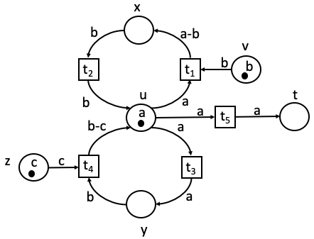
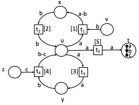
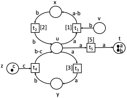
Figure 14: Out-of-causal-order reversing where $\sigma=\langle t_{\_}1,t_{\_}2,t_{\_}3,t_{\_}4,t_{\_}5\rangle$.

An example of out-of-causal-order reversibility in a cyclic RPN can be seen in Figure 14. Here the cycles $\langle t_{\_}1,t_{\_}2\rangle$ and $\langle t_{\_}3,t_{\_}4\rangle$ are executed in this order followed by transition $t_{\_}5$. We reverse in out-of-causal order transition $t_{\_}4$, which breaks the bond between $b\!-\!c$ and returns token $c$ back to its original place $z$. Moreover, the bond between $a\!-\!b$ remains in place $t$, which is the outgoing place of the last transition of token $a$. Note that this state did not occur during the forward execution of the RPN.

The following results describe how tokens and bonds are manipulated during out-of-causal-order reversibility, where we write $\stackrel{{\scriptstyle}}{{\longmapsto}}_{o}$ for $\stackrel{{\scriptstyle}}{{\longrightarrow}}\cup\stackrel{{\scriptstyle}}{{\rightsquigarrow}}_{o}$.

Proposition 7.

Suppose $\langle{M},{H}\rangle\stackrel{{\scriptstyle t}}{{\longmapsto}}_{o}\langle{M^{\prime}},{H^{\prime}}\rangle$ and let $a\in A$ where $a\in M(x)$ and $a\in M^{\prime}(y)$. Then, $\mathsf{con}(a,M^{\prime}(y))=\mathsf{con}(a,M(x)\cup C)$, where $C=\mathsf{eff}(t)\cup\{\mathsf{con}(b,M(u))\mid a-b\in\mathsf{eff}(t),b\in M(u)\})$, if $t$ is a forward transition, and $\mathsf{con}(a,M^{\prime}(y))=\mathsf{con}(a,M(x)-\mathsf{eff}(t))$, if $t$ is a reverse transition.

Proof:

The proof is straightforward by the definition of the firing rules. $\Box$

Proposition 8.

Given a reversing Petri net $(A,P,B,T,F)$, an initial state $\langle M_{\_}0,H_{\_}0\rangle$, and an execution $\langle{M_{\_}0},{H_{\_}0}\rangle\stackrel{{\scriptstyle t_{\_}1}}{{\longmapsto}}_{o}\langle{M_{\_}1},{H_{\_}1}\rangle\stackrel{{\scriptstyle t_{\_}2}}{{\longmapsto}}_{o}\ldots\stackrel{{\scriptstyle t_{\_}n}}{{\longmapsto}}_{o}\langle{M_{\_}n},{H_{\_}n}\rangle$ the following hold for all $0\leq i\leq n$:

1. For all $a\in A$, $|\{x\in P\mid a\in M_{\_}i(x)\}|=1$, and $a\in M_{\_}i(x)$ where $x=\mathsf{last}_{P}(\mathsf{con}(a,M_{\_}{i}(x)),H_{\_}i)$.

2. For all $\beta\in B$,

   1. $0\leq|\{x\in P\mid\beta\in M_{\_}i(x)\}|\leq 1$.

   2. if $|\{x\in P\mid\beta\in M_{\_}{i-1}(x)\}|=0$ and $|\{x\in P\mid\beta\in M_{\_}i(x)\}|=1$, then $t_{\_}i$ is a forward transition and $\beta\in\mathsf{eff}(t_{\_}i)$,

   3. if $|\{x\in P\mid\beta\in M_{\_}{i-1}(x)\}|=1$ and $|\{x\in P\mid\beta\in M_{\_}i(x)\}|=0$, then $t_{\_}i$ is a reverse transition and $\beta\in\mathsf{eff}(t_{\_}i)$,

   4. if $|\{x\in P\mid\beta\in M_{\_}{i-1}(x)\}|=|\{x\in P\mid\beta\in M_{\_}i(x)\}|$, then $\beta\not\in\mathsf{eff}(t_{\_}i)$.

Proof:

Consider a reversing Petri net $(A,P,B,T,F)$, an initial state $\langle M_{\_}0,H_{\_}0\rangle$, and an execution $\langle{M_{\_}0},{H_{\_}0}\rangle\stackrel{{\scriptstyle t_{\_}1}}{{\longmapsto}}_{o}\langle{M_{\_}1},{H_{\_}1}\rangle\stackrel{{\scriptstyle t_{\_}2}}{{\longmapsto}}_{o}\ldots\stackrel{{\scriptstyle t_{\_}n}}{{\longmapsto}}_{o}\langle{M_{\_}n},{H_{\_}n}\rangle$. The proof is by induction on $n$.

Base Case.

For $n=0$, by our assumption of token uniqueness and the definitions of $\mathsf{last}_{\_}P$ and $\mathsf{last}_{\_}T$ the claim follows trivially.

Induction Step.

Suppose the claim holds for all but the last transition and consider transition $t_{\_}n$. Two cases exist, depending on whether $t_{\_}n$ is a forward or a reverse transition:

• Suppose that $t_{\_}n$ is a forward transition. Then by Proposition 1, for all $a\in A$, $|\{x\in P\mid a\in M_{\_}n(x)\}|=1$. Additionally, we may see that if $a\in M_{\_}n(x)$ two cases exists. If $a\in\mathsf{con}(b,M_{\_}{n-1}(y))$, for some $b\in F(t_{\_}n,z)$ then $x=z=\mathsf{last}_{P}(\mathsf{con}(a,M_{\_}n(x)),H_{\_}n)$. Otherwise, it must be that $a\in M_{\_}{n-1}(x)$ where, by the induction hypothesis, $x=\mathsf{last}_{P}(\mathsf{con}(a,M_{\_}{n-1}(x)),H_{\_}{n-1})$. Since $a\not\in\mathsf{eff}(t_{\_}n)$, by clause 2(b) we may deduce that $\mathsf{con}(a,M_{\_}{n-1}(x))=\mathsf{con}(a,M_{\_}{n}(x))$, which leads to $x=\mathsf{last}_{P}((\mathsf{con}(a,M_{\_}{n-1}(x)),H_{\_}{n-1})=\mathsf{last}_{P}(\mathsf{con}(a,M_{\_}n(x)),H_{\_}n)$. Thus, the result follows.

  Now let $\beta\in B$. To begin with, clause (2)(a) follows by Proposition 1. Furthermore, we may see that the forward transition $t_{\_}n$ may only create exactly the bonds in $\mathsf{eff}(t_{\_}n)$ and it maintains all remaining bonds. Thus, clauses 2(b) and 2(d) follow.

• Suppose that $t_{\_}n$ is a reverse transition. Consider $a\in A$ with $a\in M_{\_}{n-1}(x)$ for some $x\in P$. Two cases exist:

  • Suppose $\mathsf{last}_{T}(\mathsf{con}(a,M_{\_}{n-1}(x)-\mathsf{eff}(t_{\_}n)),H_{\_}n)=\bot$. Then, it must be that $\mathsf{con}(a,M_{\_}{n-1}(x)-\mathsf{eff}(t_{\_}n))\subseteq M_{\_}0(y)$ for some $y$ such that $a\in M_{\_}0(y)$. Suppose that this is not the case. Then there must exist some $\beta\in\mathsf{con}(a,M_{\_}{n-1}(x)-\mathsf{eff}(t_{\_}n))$ with $\beta\not\in M_{\_}0(y)$. By the induction hypothesis, there exists some $t_{\_}i$ in the execution such that $\beta\in\mathsf{eff}(t_{\_}i)$ which was not reversed, i.e. $H_{\_}n(t_{\_}i)\neq\emptyset$. This however implies that $t_{\_}i$ is a transition that has manipulated the connected component $\mathsf{con}(a,M_{\_}{n-1}(x)-\mathsf{eff}(t_{\_}n))$, which contradicts our assumption of $\mathsf{last}_{T}(\mathsf{con}(a,M_{\_}{n-1}(x)-\mathsf{eff}(t_{\_}n)),H_{\_}n)=\bot$. Therefore, $a\in M_{\_}n(y)$, where $a\in M_{\_}0(y)$ and by Proposition 7 $\mathsf{con}(a,M_{\_}{n-1}(x)-\mathsf{eff}(t_{\_}n))=\mathsf{con}(a,M_{\_}{n}(y))$ which gives $y=\mathsf{last}_{P}(\mathsf{con}(a,M_{\_}n(y)),H_{\_}n)$ and the result follows.

  • Suppose $\mathsf{last}_{T}(\mathsf{con}(a,M_{\_}{n-1}(x)-\mathsf{eff}(t_{\_}n)),H_{\_}n)=t_{\_}k$. Then, it must be that there exists a unique $y\in t_{\_}k\circ$ such that $\mathsf{con}(a,M_{\_}{n-1}(x)-\mathsf{eff}(t_{\_}n))\cap F(t_{\_}k,z)\neq\emptyset$. Suppose that this is not the case. Then there must exist some $\beta=(a,b)\in\mathsf{con}(a,M_{\_}{n-1}(x)-\mathsf{eff}(t_{\_}n))$ with $a\in F(t_{\_}k,y_{\_}1)$, $b\in F(t_{\_}k,y_{\_}2)$, and $y_{\_}1\neq y_{\_}2$. Since $\beta\in M_{\_}n(y)$, by the induction hypothesis, there exists some $t_{\_}i$ in the execution such that $\beta\in\mathsf{eff}(t_{\_}i)$, $i>k$ which was not reversed, i.e. $H_{\_}n(t_{\_}i)\neq\emptyset$. This however implies that $t_{\_}i$ is a transition that has manipulated the connected component $\mathsf{con}(a,M_{\_}{n-1}(x)-\mathsf{eff}(t_{\_}n))$ later than $t_{\_}k$, which contradicts our assumption of $\mathsf{last}_{T}(\mathsf{con}(a,M_{\_}{n-1}(x)-\mathsf{eff}(t_{\_}n)),H_{\_}n)=t_{\_}k$. Therefore, there exists a unique $y\in t_{\_}k\circ$ such that $\mathsf{con}(a,M_{\_}{n-1}(x)-\mathsf{eff}(t_{\_}n))\cap F(t_{\_}k,z)\neq\emptyset$, $a\in M_{\_}n(y)$. Furthermore, by Proposition 7 $\mathsf{con}(a,M_{\_}{n-1}(x)-\mathsf{eff}(t_{\_}n))=\mathsf{con}(a,M_{\_}{n}(y))$ which gives $y=\mathsf{last}_{P}(\mathsf{con}(a,M_{\_}n(y)),H_{\_}n)$ and the result follows.

  Now consider $\beta\in B$. By clause 1, we may deduce clause 2(a). Finally, we may observe that the reverse transition $t_{\_}n$ may only remove exactly the bonds in $\mathsf{eff}(t_{\_}n)$ and it maintains all remaining bonds, thus, clauses 2(b)-2(d) follow. $\Box$

As we have already discussed (e.g., see Figures 2 and 14), unlike causal-order reversibility, out-of-causal-order reversibility may give rise to states that cannot be reached by forward-only execution. Nonetheless, note that the proposition establishes that during out-of-causal-order reversing it is not the case that tokens and bonds may reach places they have not previously occurred in. On the contrary, a component will always return to the place following the last transition that has manipulated it. This observation also gives rise to the following corollary, which characterises the marking of a state during computation.

Corollary 3.

Given a reversing Petri net $(A,P,B,T,F)$, an initial state $\langle M_{\_}0,H_{\_}0\rangle$, and an execution $\langle{M_{\_}0},{H_{\_}0}\rangle\stackrel{{\scriptstyle t_{\_}1}}{{\longmapsto}}_{o}\langle{M_{\_}1},{H_{\_}1}\rangle\stackrel{{\scriptstyle t_{\_}2}}{{\longmapsto}}_{o}\ldots\stackrel{{\scriptstyle t_{\_}n}}{{\longmapsto}}_{o}\langle{M_{\_}n},{H_{\_}n}\rangle$, then for all $x\in P$ we have

$$M_{\_}n(x)=\bigcup_{\_}{a\in M_{\_}n(y),\mathsf{last}_{P}(C_{\_}{a,y},H_{\_}n)=x}C_{\_}{a,y}$$

where $C_{\_}{a,y}=\mathsf{con}(a,M_{\_}n(y))$.

Proof:

According to Proposition 8 clauses (1) and 2(a) the result follows. $\Box$

The dependence of the position of a connected component and a transition sequence can be exemplified by the following proposition.

Proposition 9.

Consider executions $\langle{M_{\_}0},{H_{\_}0}\rangle\stackrel{{\scriptstyle\sigma_{\_}1}}{{\longmapsto}}_{o}\langle{M_{\_}1},{H_{\_}1}\rangle$, $\langle{M_{\_}0},{H_{\_}0}\rangle\stackrel{{\scriptstyle\sigma_{\_}2}}{{\longmapsto}}_{o}\langle{M_{\_}2},{H_{\_}2}\rangle$, and a token $a$ such that $a\in M_{\_}1(x)$, $a\in M_{\_}2(y)$, for some $x$, $y\in P$, and $\mathsf{con}(a,M_{\_}1(x))=\mathsf{con}(a,M_{\_}2(x))$. Then, $\mathsf{last}_{T}(\mathsf{con}(a,M_{\_}1(x)),H_{\_}1)=\mathsf{last}_{T}(\mathsf{con}(a,M_{\_}2(y)),H_{\_}2)$ implies $x=y$.

Proof:

Consider executions $\langle{M_{\_}0},{H_{\_}0}\rangle\stackrel{{\scriptstyle\sigma_{\_}1}}{{\longmapsto}}_{o}\langle{M_{\_}1},{H_{\_}1}\rangle$, $\langle{M_{\_}0},{H_{\_}0}\rangle\stackrel{{\scriptstyle\sigma_{\_}2}}{{\longmapsto}}_{o}\langle{M_{\_}2},{H_{\_}2}\rangle$ and a token $a$ such that $a\in M_{\_}1(x)$, $a\in M_{\_}2(x)$. Further, let us assume that $\mathsf{last}_{T}(\mathsf{con}(a,M_{\_}1(x)),H_{\_}1)=\mathsf{last}_{T}(\mathsf{con}(a,M_{\_}2(y)),H_{\_}2)$. Two cases exist:

• $\mathsf{last}_{T}(\mathsf{con}(a,M_{\_}1(x)),H_{\_}1)=\mathsf{last}_{T}(\mathsf{con}(a,M_{\_}2(y)),H_{\_}2)=\bot$. This implies that no transition has manipulated any of the tokens and bonds of the two connected components. As such, by Proposition 8, $\mathsf{con}(a,M_{\_}1(x))\subseteq M_{\_}0(x)$ and $\mathsf{con}(a,M_{\_}2(y))\subseteq M_{\_}0(y)$, and by the uniqueness of tokens we conclude that $x=y$ as required.

• $\mathsf{last}_{T}(\mathsf{con}(a,M_{\_}1(x)),H_{\_}1)=\mathsf{last}_{T}(\mathsf{con}(a,M_{\_}2(y)),H_{\_}2)=t$. This implies that there is $b\in\mathsf{con}(a,M_{\_}1(x))=\mathsf{con}(a,M_{\_}2(y))$ such that $b\in F(t,z)$ for some place $z$. By definition, we deduce that $\mathsf{last}_{P}(\mathsf{con}(a,M_{\_}1(x)),H_{\_}1)$ $=z=\mathsf{last}_{P}(\mathsf{con}(a,M_{\_}2(y)),H_{\_}2)$, thus, $x=y$ as required. $\Box$

From the above result we may prove the following proposition establishing that executing two causally equivalent sequences of transitions in the out-of-causal-order setting will give rise to causally equivalent states.

Proposition 10.

Suppose $\langle{M_{\_}0},{H_{\_}0}\rangle\stackrel{{\scriptstyle\sigma_{\_}1}}{{\longmapsto}}_{o}\langle{M_{\_}1},{H_{\_}1}\rangle$ and $\langle{M_{\_}0},{H_{\_}0}\rangle\stackrel{{\scriptstyle\sigma_{\_}2}}{{\longmapsto}}_{o}\langle{M_{\_}2},{H_{\_}2}\rangle$. If $\sigma_{\_}1\asymp\sigma_{\_}2$ then $\langle{M_{\_}1},{H_{\_}1}\rangle\asymp\langle{M_{\_}2},{H_{\_}2}\rangle$.

Proof:

Suppose $\langle{M_{\_}0},{H_{\_}0}\rangle\stackrel{{\scriptstyle\sigma_{\_}1}}{{\longmapsto}}_{o}\langle{M_{\_}1},{H_{\_}1}\rangle$, $\langle{M_{\_}0},{H_{\_}0}\rangle\stackrel{{\scriptstyle\sigma_{\_}2}}{{\longmapsto}}_{o}\langle{M_{\_}2},{H_{\_}2}\rangle$ and $\sigma_{\_}1\asymp\sigma_{\_}2$. Since $\sigma_{\_}1\asymp\sigma_{\_}2$ it must be that the two executions contain the same causal paths, therefore, $H_{\_}1\asymp H_{\_}2$. To show that $M_{\_}1=M_{\_}2$ consider token $a$ such that $a\in M_{\_}1(x)\cap M_{\_}2(y)$. Since $\sigma_{\_}1\asymp\sigma_{\_}2$, we may conclude that the two executions contain the same set of executed and not reversed transitions. Thus, by Proposition 8(2), we have $\mathsf{con}(a,M_{\_}1(x))=\mathsf{con}(a,M_{\_}2(y))$. Furthermore, it must be that $t_{\_}1=\mathsf{last}_{T}(\mathsf{con}(a,M_{\_}1(x)),H_{\_}1)=\mathsf{last}_{T}(\mathsf{con}(a,M_{\_}2(y)),H_{\_}2)=t_{\_}2$. If not, since $\sigma_{\_}1\asymp\sigma_{\_}2$, we would have that $t_{\_}1$ and $t_{\_}2$ are concurrent, which is not possible since they manipulate the same connected component and thus a causal relation exists between them. Therefore, by Proposition 9, $x=y$. This implies by Corollary 3 that $M_{\_}1(x)=M_{\_}2(x)$, for all places $x$, which completes the proof. $\Box$

We finally establish a Loop Lemma for out-of-causal reversibility.

Lemma 5 (Loop).

For any forward transition $\langle{M},{H}\rangle\stackrel{{\scriptstyle t}}{{\longrightarrow}}\langle{M^{\prime}},{H^{\prime}}\rangle$ there exists a reverse transition $\langle{M^{\prime}},{H^{\prime}}\rangle\stackrel{{\scriptstyle t}}{{\rightsquigarrow}}_{o}\langle{M},{H}\rangle$.

Proof:

Suppose $\langle{M},{H}\rangle\stackrel{{\scriptstyle t}}{{\longrightarrow}}\langle{M^{\prime}},{H^{\prime}}\rangle$. Then $t$ is clearly $o$-enabled in $H^{\prime}$. Furthermore, $\langle{M^{\prime}},{H^{\prime}}\rangle\stackrel{{\scriptstyle t}}{{\rightsquigarrow}}_{o}\langle{M^{\prime\prime}},{H^{\prime\prime}}\rangle$ where $H^{\prime\prime}=H$ by the definition of $\stackrel{{\scriptstyle}}{{\rightsquigarrow}}_{o}$. In addition, for all $a\in A$, we may prove that $a\in M^{\prime\prime}(x)$ if and only if $a\in M(x)$. Suppose $a\in M(y)$, we distinguish two cases. If $\mathsf{con}(a,M(y))\cap\mathsf{pre}(t)=\emptyset$, then we may see that $a\in M^{\prime}(y)$ and $a\in M^{\prime\prime}(y)$, and the result follows. Otherwise, if $\mathsf{con}(a,M(y))\cap\mathsf{pre}(t)\neq\emptyset$, then $a\in M^{\prime}(z)$, where $F(t,z)\cap\mathsf{con}(a,M(y))\neq\emptyset$. Furthermore, suppose that $a\in M^{\prime\prime}(w)$. By Proposition 7 we have that $\mathsf{con}(a,M^{\prime}(z))=\mathsf{con}(a,M(y)\cup C)$, $C=\mathsf{eff}(t)\cup\{\mathsf{con}(b,M(u))\mid a-b\in\mathsf{eff}(t),b\in M(u)\}$, and $\mathsf{con}(a,M^{\prime\prime}(w))=\mathsf{con}(a,M^{\prime}(z)-\mathsf{eff}(t))=\mathsf{con}(a,(M(y)\cup C)-\mathsf{eff}(t))=\mathsf{con}(a,M(y))$. Furthermore, $y=\mathsf{last}_{P}(\mathsf{con}(a,M(y)),H)$, by Corollary 3. Since $H=H^{\prime\prime}$, we have $w=\mathsf{last}_{P}(\mathsf{con}(a,M^{\prime\prime}(w)),H^{\prime\prime}))=\mathsf{last}_{P}(\mathsf{con}(a,M(y)),H))=y$, and the result follows. $\Box$

Note that in the case of out-of-causal-order reversibility, the opposite direction of the lemma does not hold. This is because reversing a transition in an out-of-causal-order fashion may bring a system to a state not reachable by forward-only transitions, and where the transition is not enabled in the forward direction. As an example, consider the RPN of Figure 13 and after the reversal of transition $t_{\_}2$. In this state, transition $t_{\_}2$ is not forward enabled since token $b$ is not available in place $x$, as required for the transition to fire.

5.4 Relationship between reversibility notions

We continue to study the relationship between the three forms of reversibility. Our first result confirms the relationship between the enabledness conditions for each of backtracking, causal-order, and out-of-causal-order reversibility.

Proposition 11.

Consider a state $\langle M,H\rangle$, and a transition $t$. Then, if $t$ is $bt$-enabled in $\langle M,H\rangle$ it is also $co$-enabled. Furthermore, if $t$ is $co$-enabled in $\langle M,H\rangle$ then it is also $o$-enabled.

Proof:

The proof is immediate by the respective definitions. $\Box$

We next demonstrate a “universality” result of the $\stackrel{{\scriptstyle}}{{\rightsquigarrow}}_{o}$ transition relation by showing that it manipulates the state of a reversing Petri net in an identical way to $\stackrel{{\scriptstyle}}{{\rightsquigarrow}}_{c}$, in the case of $co$-enabled transitions, and to $\stackrel{{\scriptstyle}}{{\rightsquigarrow}}_{b}$, in the case of $bt$-enabled transitions. Central to the proof is the following result establishing that during causal-order reversibility a component is returned to the place following the last transition that has manipulated it or, if no such transition exists, in the place where it occurred in the initial marking.

Proposition 12.

Given a reversing Petri net $(A,P,B,T,F)$, an initial state $\langle M_{\_}0,H_{\_}0\rangle$, and an execution $\langle{M_{\_}0},{H_{\_}0}\rangle\stackrel{{\scriptstyle t_{\_}1}}{{\longmapsto}}_{c}\langle{M_{\_}1},{H_{\_}1}\rangle\stackrel{{\scriptstyle t_{\_}2}}{{\longmapsto}}_{c}\ldots\stackrel{{\scriptstyle t_{\_}n}}{{\longmapsto}}_{c}\langle{M_{\_}n},{H_{\_}n}\rangle$. Then for all $a\in A$, $a\in M_{\_}n(x)$ where $x=\mathsf{last}_{P}(\mathsf{con}(a,M_{\_}{n}(x)),H_{\_}n)$.

Proof:

The proof is by induction on $n$ and it follows along similar lines to the proof of Proposition 8(1). $\Box$

Propositions 8 and 12 yield the following corollary for forward-only execution.

Corollary 4.

Given a reversing Petri net $(A,P,B,T,F)$, an initial state $\langle M_{\_}0,H_{\_}0\rangle$, and an execution $\langle{M_{\_}0},{H_{\_}0}\rangle\stackrel{{\scriptstyle t_{\_}1}}{{\longrightarrow}}\langle{M_{\_}1},{H_{\_}1}\rangle\stackrel{{\scriptstyle t_{\_}2}}{{\longrightarrow}}\ldots\stackrel{{\scriptstyle t_{\_}n}}{{\longrightarrow}}\langle{M_{\_}n},{H_{\_}n}\rangle$, for all $a\in A$, $a\in M_{\_}n(x)$ where $x=\mathsf{last}_{P}(\mathsf{con}(a,M_{\_}{n}(x)),H_{\_}n)$.

We may now verify that the causal-order and out-of-causal-order reversibility have the same effect when reversing a $co$-enabled transition.

Proposition 13.

Consider a state $\langle M,H\rangle$ and a transition $t$ $co$-enabled in $\langle M,H\rangle$. Then, $\langle M,H\rangle\stackrel{{\scriptstyle t}}{{\rightsquigarrow}}_{c}\langle M^{\prime},H^{\prime}\rangle$ if and only if $\langle M,H\rangle\stackrel{{\scriptstyle t}}{{\rightsquigarrow}}_{o}\langle M^{\prime},H^{\prime}\rangle$.

Proof:

Let us suppose that transition $t$ is $co$-enabled and $\langle M,H\rangle\stackrel{{\scriptstyle t}}{{\rightsquigarrow}}_{c}\langle M_{\_}1,H_{\_}1\rangle$. By Proposition 11, $t$ is also $o$-enabled. Suppose $\langle M,H\rangle\stackrel{{\scriptstyle t}}{{\rightsquigarrow}}_{o}\langle M_{\_}2,H_{\_}2\rangle$. It is easy to see that in fact $H_{\_}1=H_{\_}2$ (the two histories are as $H$ with the exception that $H_{\_}1(t)=H_{\_}2(t)=H(t)-\{\max(H(t))\}$).

To show that $M_{\_}1=M_{\_}2$ first we observe that for all $a\in A$, by Proposition 12 we have $a\in M_{\_}1(x)$ where $x=\mathsf{last}_{P}(\mathsf{con}(a,M_{\_}1(x)),H_{\_}1)$ and by Proposition 8 we have $a\in M_{\_}1(y)$ where $y=\mathsf{last}_{P}(\mathsf{con}(a,M_{\_}2(y)),H_{\_}2)$. We may also see that $\mathsf{con}(a,M_{\_}1(x))=\mathsf{con}(a,M(z)-\mathsf{eff}(t))=\mathsf{con}(a,M_{\_}2(y))$, where $a\in M(z)$. Since in addition we have $H_{\_}1=H_{\_}2$ the result follows.

Now let $\beta\in B$. We must show that $\beta\in M_{\_}1(x)$ if and only if $\beta\in M_{\_}2(x)$. Two cases exist:

• If $\beta\in\mathsf{eff}(t)$ then by Propositions 4 and 8, $\beta\not\in M_{\_}1(x)$ and $\beta\not\in M_{\_}2(x)$ for all $x\in P$.

• if $\beta\not\in\mathsf{eff}(t)$ then by Propositions 4 and 8, $|\{x\in P\mid\beta\in M_{\_}1(x))\}|=|\{x\in P\mid\beta\in M_{\_}2(x))\}|=1$ and by the analysis on tokens $\beta\in M_{\_}1(x)$ if and only if $\beta\in M_{\_}2(x)$ and the result follows.

This completes the proof. $\Box$

An equivalent result can be obtained for backtracking.

Proposition 14.

Consider a state $\langle M,H\rangle$, and a transition $t$, $bt$-enabled in $\langle M,H\rangle$. Then, $\langle M,H\rangle\stackrel{{\scriptstyle t}}{{\rightsquigarrow}}_{b}\langle M^{\prime},H^{\prime}\rangle$ if and only if $\langle M,H\rangle\stackrel{{\scriptstyle t}}{{\rightsquigarrow}}_{o}\langle M^{\prime},H^{\prime}\rangle$.

Proof:

Consider a state $\langle M,H\rangle$ and suppose that transition $t$ is $bt$-enabled and $\langle M,H\rangle\stackrel{{\scriptstyle t}}{{\rightsquigarrow}}_{b}\langle M^{\prime},H^{\prime}\rangle$. Then, by Proposition 11, there exists $k\in H(t)$, such that for all $t^{\prime}\in T$, $k^{\prime}\in H(t^{\prime})$, it holds that $k\geq k^{\prime}$. This implies that $t$ is also $co$-enabled, and by the definition of $\stackrel{{\scriptstyle}}{{\rightsquigarrow}}_{c}$, we conclude that $\langle M,H\rangle{\stackrel{{\scriptstyle t}}{{\rightsquigarrow}}_{c}}\langle M^{\prime},H^{\prime}\rangle$. Furthermore, by Proposition 13 $\langle M,H\rangle{\stackrel{{\scriptstyle t}}{{\rightsquigarrow}}_{o}}\langle M^{\prime},H^{\prime}\rangle$, and the result follows. $\Box$

We obtain the following corollary confirming the expectation that backtracking is an instance of causal reversing, which in turn is an instance of out-of-causal-order reversing. It is easy to see that both inclusions are strict, as for example illustrated in Figures 5, 9, and 13.

Corollary 5.

$\stackrel{{\scriptstyle}}{{\rightsquigarrow}}_{b}\subset\stackrel{{\scriptstyle}}{{\rightsquigarrow}}_{c}\subset\stackrel{{\scriptstyle}}{{\rightsquigarrow}}_{o}$.

Proof:

The proof follows from Propositions 13 and 14. $\Box$

We note that in addition to establishing the relationship between the three notions of reversibility, the above results provide a unification of the different reversal strategies, in the sense that a single firing rule, $\stackrel{{\scriptstyle}}{{\rightsquigarrow}}_{o}$, may be paired with the three notions of transition enabledness to provide the three different notions of reversibility. This fact may be exploited in the proofs of results that span the three notions of reversibility. Such a proof follows in the following proposition that establishes a reverse diamond property for RPNs. According to this property, the execution of a reverse transition does not preclude the execution of another reverse transition and their execution leads to the same state. In what follows we write $\stackrel{{\scriptstyle}}{{\longmapsto}}$ for $\stackrel{{\scriptstyle}}{{\longrightarrow}}\cup\stackrel{{\scriptstyle}}{{\rightsquigarrow}}$ where $\stackrel{{\scriptstyle}}{{\rightsquigarrow}}$ could be an instance of one of $\stackrel{{\scriptstyle}}{{\rightsquigarrow}}_{b}$, $\stackrel{{\scriptstyle}}{{\rightsquigarrow}}_{c}$, and $\stackrel{{\scriptstyle}}{{\rightsquigarrow}}_{o}$.

Proposition 15 (Reverse Diamond).

Consider a state $\langle{M},{H}\rangle$, and reverse transitions $\langle{M},{H}\rangle\stackrel{{\scriptstyle t_{\_}1}}{{\rightsquigarrow}}\langle{M_{\_}1},{H_{\_}1}\rangle$ and $\langle{M},{H}\rangle\stackrel{{\scriptstyle t_{\_}2}}{{\rightsquigarrow}}\langle{M_{\_}2},{H_{\_}2}\rangle$, $t_{\_}1\neq t_{\_}2$. Then $\langle{M_{\_}1},{H_{\_}1}\rangle\stackrel{{\scriptstyle t_{\_}2}}{{\rightsquigarrow}}\langle{M^{\prime}},{H^{\prime}}\rangle$ and $\langle{M_{\_}2},{H_{\_}2}\rangle\stackrel{{\scriptstyle t_{\_}1}}{{\rightsquigarrow}}\langle{M^{\prime}},{H^{\prime}}\rangle.$

Proof:

Let us suppose that $\langle{M},{H}\rangle\stackrel{{\scriptstyle t_{\_}1}}{{\rightsquigarrow}}\langle{M_{\_}1},{H_{\_}1}\rangle$ and $\langle{M},{H}\rangle\stackrel{{\scriptstyle t_{\_}2}}{{\rightsquigarrow}}\langle{M_{\_}2},{H_{\_}2}\rangle$, $t_{\_}1\neq t_{\_}2$. First we note that $\stackrel{{\scriptstyle}}{{\rightsquigarrow}}$ may be an instance of $\stackrel{{\scriptstyle}}{{\rightsquigarrow}}_{c}$ or $\stackrel{{\scriptstyle}}{{\rightsquigarrow}}_{o}$ but not $\stackrel{{\scriptstyle}}{{\rightsquigarrow}}_{b}$, since in the case of $\stackrel{{\scriptstyle}}{{\rightsquigarrow}}_{b}$ the backward transition is uniquely determined as the transition with the maximum key. Furthermore, we observe that $t_{\_}2$ remains backward-enabled in $\langle{M_{\_}1},{H_{\_}1}\rangle$ and likewise $t_{\_}1$ in $\langle{M_{\_}2},{H_{\_}2}\rangle$. Specifically, if $\stackrel{{\scriptstyle}}{{\rightsquigarrow}}=\stackrel{{\scriptstyle}}{{\rightsquigarrow}}_{c}$, since $t_{\_}1$ and $t_{\_}2$ are $co-$enabled in $\langle{M},{H}\rangle$, by Definition 10 we conclude that $(t_{\_}2,max(H(t_{\_}2)))$ is not causally dependent on $(t_{\_}1,max(H(t_{\_}1)))$ and vice versa, which continues to hold after the reversal of each of these transitions. In the case of $\stackrel{{\scriptstyle}}{{\rightsquigarrow}}=\stackrel{{\scriptstyle}}{{\rightsquigarrow}}_{o}$ this is straightforward from the definition of $o$-enabledness.

So, let us suppose that $\langle{M_{\_}1},{H_{\_}1}\rangle\stackrel{{\scriptstyle t_{\_}2}}{{\rightsquigarrow}}_{c}\langle{M_{\_}1^{\prime}},{H_{\_}1^{\prime}}\rangle$ and $\langle{M_{\_}2},{H_{\_}2}\rangle\stackrel{{\scriptstyle t_{\_}1}}{{\rightsquigarrow}}_{c}\langle{M_{\_}2^{\prime}},{H_{\_}2^{\prime}}\rangle$. It is easy to see that $H_{\_}1^{\prime}=H_{\_}2^{\prime}$ since both of these histories are identical with $H$ with the maximum keys of $t_{\_}1$ and $t_{\_}2$ removed.

To show that $M_{\_}1^{\prime}=M_{\_}2^{\prime}$ first we observe that for all $a\in A$, by Propositions 8 and 12 we have $a\in M_{\_}1^{\prime}(x)$, $a\in M_{\_}2^{\prime}(y)$ where $x=\mathsf{last}_{P}(\mathsf{con}(a,M_{\_}1^{\prime}(x)),$ $H_{\_}1^{\prime})$ and $y=\mathsf{last}_{P}(\mathsf{con}(a,M_{\_}2^{\prime}(y)),H_{\_}2^{\prime})$. We may see that $\mathsf{con}(a,M_{\_}1^{\prime}(x))=\mathsf{con}(a,M(z)-(\mathsf{eff}(t_{\_}1)\cup\mathsf{eff}(t_{\_}2))=\mathsf{con}(a,M_{\_}2^{\prime}(y))$, where $a\in M(z)$. Since in addition we have $H_{\_}1^{\prime}=H_{\_}2^{\prime}$ the result follows.

Now let $\beta\in B$. We must show that $\beta\in M_{\_}1^{\prime}(x)$ if and only if $\beta\in M_{\_}2^{\prime}(x)$. Two cases exist:

• If $\beta\in\mathsf{eff}(t_{\_}1)\cup\mathsf{eff}(t_{\_}2)$ then by Propositions 4 and 8, $\beta\not\in M_{\_}1^{\prime}(x)$ and $\beta\not\in M_{\_}2^{\prime}(x)$ for all $x\in P$.

• if $\beta\not\in\mathsf{eff}(t_{\_}1)\cup\mathsf{eff}(t_{\_}2)$ then by Propositions 4 and 8, $|\{x\in P\mid\beta\in M_{\_}1^{\prime}(x))\}|=|\{x\in P\mid\beta\in M_{\_}2^{\prime}(x))\}|$ and, by the analysis on tokens, $\beta\in M_{\_}1^{\prime}(x)$ if and only if $\beta\in M_{\_}2^{\prime}(x)$.

This completes the proof. $\Box$

Corollary 6.

Consider a state $\langle{M},{H}\rangle$, and traces $\sigma_{\_}1,\sigma_{\_}2$ permutations of the same reverse transitions where $\langle{M},{H}\rangle\stackrel{{\scriptstyle\sigma_{\_}1}}{{\longmapsto}}\langle{M^{\prime}},{H^{\prime}}\rangle$ and $\langle{M},{H}\rangle\stackrel{{\scriptstyle\sigma_{\_}2}}{{\longmapsto}}\langle{M^{\prime\prime}},{H^{\prime\prime}}\rangle$. Then $\langle{M^{\prime}},{H^{\prime}}\rangle=\langle{M^{\prime\prime}},{H^{\prime\prime}}\rangle$.

Proof:

The proof follows by induction on the sum of the length $|\sigma_{\_}1|=|\sigma_{\_}2|$ and the depth of the earliest disagreement between the two traces, and uses similar arguments to those found in the proof of Proposition 15. $\Box$

We note that the analogue of Proposition 15 for forward transitions, i.e. the Forward Diamond property, does not hold for RPNs. To begin with $t_{\_}1$ and $t_{\_}2$ may be in conflict. The proposition fails to hold even in the case of joinable transitions (i.e. transitions that may yield the same marking after a sequence of forward moves) due to the case of co-initial, independent cycles: Even though such cycles can be executed in any order, it is impossible to complete the square for their initial transitions.

6 Case Study

Biochemical systems, such as covalent bonds, constitute the ideal setting to study reversible computation especially in its out-of-causal-order form. In particular, the ERK signalling pathway is one of many real-life examples that naturally feature reversibility that violates the causal ordering established by forward execution. This pathway has been modelled in various formalisms including CCSK [24], PEPA [6], BioNetGen [5], and Kappa [9]. In this section we illustrate how reversing Petri nets allow us to capture naturally this form of out-of-causal-order reversible system.

In Figure 15 we demonstrate the extracellular-signal-regulated kinase (ERK) pathway, also known as Ras/Raf-1, MEK, ERK pathway, which is one of the major signalling cassettes of the mitogen activated protein kinase (EMAPK) signalling pathway. The ERK pathway is a chain of proteins in the cell that delivers mitogenic and differentiation signals from the membrane of a cell to the DNA in the nucleus, and is regulated by the protein RKIP. The starting point of the pathway is when a signalling molecule binds to a receptor on the cell surface and is spatially organised so that, when a signal arrives at the membrane, it can be transmitted to the nucleus via a cascade of biological reactions that involves protein kinases. A kinase is an enzyme that catalyses the transfer of a phosphate group from a donor molecule to an acceptor. The main $\mathit{MAPK/ERK}$ kinase kinase (MEKK) component is the kinase component Raf-1 that phosphorylates the serine residue on the MAPK/ERK kinase MEK. We denote Raf*-1 with F, MEK with M, ERK with E, RKIP with R, and the phosphorylation of the bonded molecule is denoted by P.

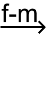
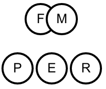
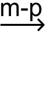
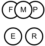
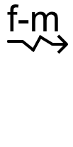
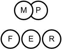
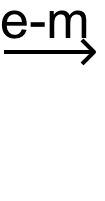
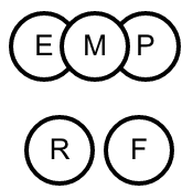
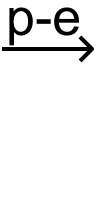
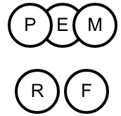
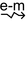
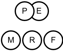
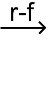
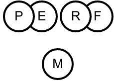
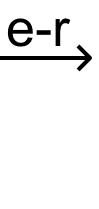
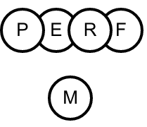
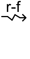
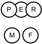
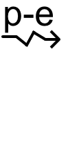
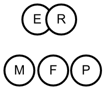
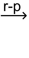
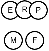
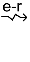
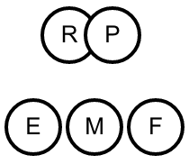
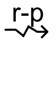
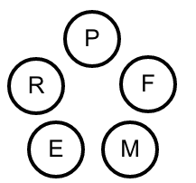
Figure 15: Reactions in the ERK-pathway where F denotes Raf*-1, M denotes MEK, E denotes ERK, R denotes RKIP, and P denotes the phosphorylation of the bonded molecule.

The pathway begins with the activation of the protein kinase of Raf-1 by the $G$ protein Ras that has been activated near a receptor on the cell’s membrane. Ras activates a kinase Raf-1 to become Raf*-1, which is generally known as a mitogen-activated protein kinase kinase kinase (MAP-KKK) and can be inhibited by RKIP. Subsequently, as we may see in Figure 15, Raf*-1 ($F$) may bind with MEK ($F\!-\!M$) by facilitating the next step in the cascade (MAPKK), which is the phosphorylation of the MEK ($F\!-\!M\!-\!P$) protein and the release of Raf*-1 ($M\!-\!P$). The phosphorylated MEK ($M\!-\!P$) activates a mitogen-activated protein kinase, ERK ($E\!-\!M\!-\!P$), which in turn becomes phosphorylated and releases MEK ($P\!-\!E$). Finally, the phosphorylation of MAPK allows the phosphorylated ERK ($P\!-\!E$) to function as an enzyme and translocate in order to signal the nucleus. Now the regulation sequence consumes the phosphorylated ERK ($P\!-\!E$) in order to deactivate RKIP ($R$) from regulating Raf*-1 ($F$). Therefore, when RKIP binds Raf*-1 ($R\!-\!F$), the resulting complex binds to a phosphorylated ERK ($P\!-\!E\!-\!R\!-\!F$). In the end, the complex breaks releasing Raf*-1 ($P\!-\!E\!-\!R$), which can get involved in the cascade and after the phosphorylation of RKIP ($E\!-\!R\!-\!P$) the system releases ERK ($R\!-\!P$) and the phosphorylated RKIP.

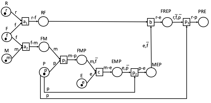
Figure 16: ERK-pathway example in Reversing Petri Nets

We now describe the biochemical reactions of the ERK signalling pathway as the RPN demonstrated in Figure 16. On this RPN we represent molecules as tokens that can bond with each other, thus creating more complex molecules, and these composite molecules can be dissolved back to single tokens. The building blocks of the system are the base tokens representing the associated molecules.

We begin our execution from the already activated Raf-1 kinase that has become Raf*-1. The molecule of Raf*-1 is represented by base token $f$ and resides in place $F$. The token availability of base $m$, which represents MEK in place $M$ enables the firing of transition $a_{\_}2$ denoting that $f$ has bonded with $m$ and thus creating molecule $f\!-\!m$. The firing of transition $a_{\_}2$ facilitates the next step in the cascade, which is transition $p_{\_}1$ representing the phosphorylation of $m$ as the binding between $p$ and $m$. Since transition $a_{\_}2$ has enabled the execution of $p_{\_}1$ the transition $a_{\_}2$ is now reversed and therefore releases $f$ back to place $F$. This reversal in necessary for the next step of the execution where the absence of $f$ is a condition for transition $c$ to fire. Indeed, in transition $c$, the phosphorylated $m$ is now able to activate the kinase ERK denoted by base $e$ and thus creating a bond between $m\!-\!e$ along with $p$ that shows that $m$ is already phosphorylated. In the next step, transition $p_{\_}1$ reverses in order to release $p$, which can then be used in the firing of transition $p_{\_}2$ to phosphorylate $e$ and therefore creating the molecule $p\!-\!e$. After transition $p_{\_}2$ transition $c$ is reversed in order to release $m$ back to $M$. Finally, after the phosphorylation of $p\!-\!e$, transition $a_{\_}1$ executes in order to bond $f\!-\!r$ where $r$ represents molecule $RKIP$. Base $r$ functions as an enzyme and by enabling transition $b$ represents the passing of the signal to the nucleus which can then consume $p\!-\!e$ by creating a connected component between $f\!-\!r\!-\!e\!-\!p$. In the end, the complex breaks by reversing $a_{\_}1$ in order to release $f$ and $p_{\_}2$ to release $p$ which then in action $p_{\_}3$ phosphorylates $r$. Finally, the system reverses $b$ to release $e$ followed by the reversal of $p_{\_}3$, which releases both $r$ and $p$ and therefore returns the system back to its initial marking.

We show below an execution of the reversing Petri net that illustrates the process until the signal that arrived at the membrane is transmitted to the nucleus. The following states of the net (with histories omitted) represent a cascade of reactions that involve protein kinases $F$, $M$, $E$, $P$, $R$, with initial marking $M_{\_}0$ such that $M_{\_}0(R)=\{r\}$, $M_{\_}0(F)=\{f\}$, $M_{\_}0(M)=\{m\}$, $M_{\_}0(P)=\{p\}$, $M_{\_}0(E)=\{e\}$, and $M_{\_}0(p)=\emptyset$ for all remaining places. (In the following, the markings of places with no tokens are omitted.)

$M_{\_}0\xrightarrow{a_{\_}2}M_{\_}1$,	where	$M_{\_}1(R)=\{r\}$, $M_{\_}1(P)=\{p\}$, $M_{\_}1(E)=\{e\}$,
$M_{\_}1(FM)=\{f\!-\!m\}$
$M_{\_}1\xrightarrow{p_{\_}1}M_{\_}2$,	where	$M_{\_}2(R)=\{r\}$, $M_{\_}2(E)=\{e\}$,
$M_{\_}2(FMP)=\{f\!-\!m,m\!-\!p\}$
$M_{\_}2\stackrel{{\scriptstyle a_{\_}2}}{{\rightsquigarrow}}M_{\_}3$,	where	$M_{\_}3(R)=\{r\}$, $M_{\_}3(F)=\{f\}$, $M_{\_}3(E)=\{e\}$,
$M_{\_}3(FMP)=\{m\!-\!p\}$
$M_{\_}3\xrightarrow{c}M_{\_}4$,	where	$M_{\_}4(R)=\{r\}$, $M_{\_}4(F)=\{f\}$,
$M_{\_}4(EMP)=\{m\!-\!e,m\!-\!p\}$
$M_{\_}4\stackrel{{\scriptstyle p_{\_}1}}{{\rightsquigarrow}}M_{\_}5$,	where	$M_{\_}5(R)=\{r\}$, $M_{\_}5(F)=\{f\}$, $M_{\_}5(P)=\{p\}$,
$M_{\_}5(EMP)=\{m\!-\!e\}$
$M_{\_}5\xrightarrow{p_{\_}2}M_{\_}6$,	where	$M_{\_}6(R)=\{r\}$, $M_{\_}6(F)=\{f\}$,
$M_{\_}6(MEP)=\{m\!-\!e,e\!-\!p\}$
$M_{\_}6\stackrel{{\scriptstyle c}}{{\rightsquigarrow}}M_{\_}7$,	where	$M_{\_}7(R)=\{r\}$, $M_{\_}7(F)=\{f\}$, $M_{\_}7(M)=\{m\}$,
$M_{\_}7(MEP)=\{e\!-\!p\}$
$M_{\_}7\xrightarrow{a_{\_}1}M_{\_}8$,	where	$M_{\_}8(M)=\{m\}$, $M_{\_}8(RF)=\{r\!-\!f\}$,
$M_{\_}8(MEP)=\{e\!-\!p\}$
$M_{\_}8\xrightarrow{b}M_{\_}9$,	where	$M_{\_}9(M)=\{m\}$, $M_{\_}9(FREP)=\{r\!-\!f,r\!-\!e,e\!-\!p\}$
$M_{\_}9\stackrel{{\scriptstyle a_{\_}1}}{{\rightsquigarrow}}M_{\_}{10}$,	where	$M_{\_}{10}(M)=\{m\}$, $M_{\_}{10}(F)=\{f\}$,
$M_{\_}{10}(FREP)=\{r\!-\!e,e\!-\!p\}$
$M_{\_}{10}\stackrel{{\scriptstyle p_{\_}2}}{{\rightsquigarrow}}M_{\_}{11}$,	where	$M_{\_}{11}(M)=\{m\}$, $M_{\_}{11}(F)=\{f\},M_{\_}{11}(P)=\{p\}$,
$M_{\_}{11}(FREP)=\{r\!-\!e\}$
$M_{\_}{11}\xrightarrow{p_{\_}3}M_{\_}{12}$,	where	$M_{\_}{12}(M)=\{m\}$, $M_{\_}{12}(F)=\{f\}$,
$M_{\_}{12}(PRE)=\{r\!-\!e,p\!-\!r\}$
$M_{\_}{12}\stackrel{{\scriptstyle b}}{{\rightsquigarrow}}M_{\_}{13}$,	where	$M_{\_}{13}(M)=\{m\}$, $M_{\_}{13}(F)=\{f\}M_{\_}{13}(E)\{e\}$,
$M_{\_}{13}(PRE)=\{p\!-\!r\}$
$M_{\_}{13}\stackrel{{\scriptstyle p3}}{{\rightsquigarrow}}M_{\_}{14}$,	where	$M_{\_}{14}(R)=\{r\}$, $M_{\_}{14}(F)=\{f\}$, $M_{\_}{14}(M)=\{m\}$,
$M_{\_}{14}(P)=\{p\}$, $M_{\_}{14}(E)=\{e\}$

7 Conclusions

This paper proposes a reversible approach to Petri nets that allows the modelling of reversibility as realised by backtracking, causal-order reversing and out-of-causal-order reversing. To the best of our knowledge, this is the first such proposal in the context of Petri nets. For instance, the work of [2, 3] introduces reversed transitions in a Petri net and studies various decidability problems in this setting. This approach, however, does not precisely capture reversible behavior due to the property of backward conflict in PNs. Moreover, the work of [19] proposes a causal semantics for P/T nets by identifying the causalities and conflicts of a P/T net through unfolding it into an equivalent occurrence net and subsequently introducing appropriate reverse transitions to create a coloured Petri net that captures a causal-consistent reversible semantics. The colours in this net capture causal histories. On the other hand, our proposal consists of a reversible approach to Petri nets, where the formalism supports the reversible semantics without explicitly introducing reverse transitions. This is achieved with the use of bonds of tokens, which can be thought of as colours and, combined with the history function of the semantics, capture the memory of an execution as needed to implement reversibility. Furthermore, the approach allows to implement both causal-order and out-of-causal-order reversibility.

A main main contribution of this work has been the addition of cycles in the RPN model of [21]. To enable this, additional machinery has been necessary to capture causal dependencies in the presence of cycles. As also in [19], our goal has been to allow a causally-consistent semantics reflecting causal dependencies as a partial order, and allowing an event to be reversed only if all its consequences have already been undone. To achieve this goal we have defined a causal dependence relation that resorts to the marking of a net. As illustrated via examples (e.g. see Figures 7 and 8), this is central in capturing causal dependencies and the intended causal-consistent semantics.

In a related line of work, we are also investigating the expressiveness relationship between RPNs and CPNs. Specifically, in [1] a subclass of RPNs with trans-acyclic structures has been encoded in coloured PNs. Currently, we are extending this work with ultimate objective to provide and prove the correctness of the translation between the two formalisms and analyse the associated trade-offs in terms of Petri net size.

Controlling reversibility in RPNs is another topic of current work. Specifically, in [22, 27] we have extended RPNs with conditions that control reversibility, and we have applied our framework in the context of wireless communications. This experience has illustrated that resource management can be studied and understood in terms of RPNs as, along with their visual nature, they offer a number of features, such as token persistence, that is especially relevant in these contexts. In future work, we would like to further apply our framework in the specific fields as well as in the fields of biochemistry and long-running transactions.

Finally, our current work focuses on relaxing the remaining restrictions of RPNS, to allow multiple tokens of the same base/type to occur in a model and to develop reversible semantics in the presence of bond destruction.

Acknowledgents:

This research was partially supported by the EU COST Action IC1405.

References

- [1] K. Barylska, A. Gogolinska, L. Mikulski, A. Philippou, M. Piatkowski, and K. Psara. Reversing computations modelled by coloured Petri nets. In Proceedings ATAED 2018, pages 91–111, 2018.
- [2] K. Barylska, M. Koutny, L. Mikulski, and M. Piatkowski. Reversible computation vs. reversibility in Petri nets. In Proceedings of RC 2016, LNCS 9720, pages 105–118. Springer, 2016.
- [3] K. Barylska, L. Mikulski, M. Piatkowski, M. Koutny, and E. Erofeev. Reversing transitions in bounded Petri nets. In Proceedings of CS&P 2016, volume 1698 of CEUR Workshop Proceedings, pages 74–85, 2016.
- [4] G. Berry and G. Boudol. The chemical abstract machine. Theoretical Computer Science, 96(1):217–248, 1992.
- [5] M. L. Blinov, J. Yang, J. R. Faeder, and W. S. Hlavacek. Graph theory for rule-based modeling of biochemical networks. Transactions on Computational Systems Biology VII, pages 89–106, 2006.
- [6] M. Calder, S. Gilmore, and J. Hillston. Modelling the influence of RKIP on the ERK signalling pathway using the stochastic process algebra PEPA. In Transactions on Computational Systems Biology, LNCS 4230, pages 1–23. Springer, 2006.
- [7] L. Cardelli and C. Laneve. Reversible structures. In Proceedings of CMSB 2011, pages 131–140. ACM, 2011.
- [8] I. Cristescu, J. Krivine, and D. Varacca. A compositional semantics for the reversible pi-calculus. In Proceedings of ACM/IEEE 2013, pages 388–397, 2013.
- [9] V. Danos, J. Feret, W. Fontana, R. Harmer, and J. Krivine. Rule-based modelling of cellular signalling. In Proceedings of CONCUR 2007, LNCS 4703, pages 17–41. Springer, 2007.
- [10] V. Danos and J. Krivine. Reversible communicating systems. In Proceedings of CONCUR 2004, LNCS 3170, pages 292–307. Springer, 2004.
- [11] V. Danos and J. Krivine. Transactions in RCCS. In Proceedings of CONCUR 2005, LNCS 3653, pages 398–412. Springer, 2005.
- [12] V. Danos and J. Krivine. Formal molecular biology done in CCS-R. Electronic Notes in Theoretical Computer Science, 180(3):31–49, 2007.
- [13] V. Danos, J. Krivine, and P. Sobocinski. General reversibility. Electronic Notes in Theoretical Computer Science, 175(3):75–86, 2007.
- [14] S. Kuhn and I. Ulidowski. A calculus for local reversibility. In Proceedings of RC 2016, LNCS 9720, pages 20–35. Springer, 2016.
- [15] R. Landauer. Irreversibility and heat generation in the computing process. IBM Journal of Research and Development, 5(3):183–191, 1961.
- [16] I. Lanese, M. Lienhardt, C. A. Mezzina, A. Schmitt, and J. Stefani. Concurrent flexible reversibility. In Proceedings of ESOP 2013, LNCS 7792, pages 370–390. Springer, 2013.
- [17] I. Lanese, C. A. Mezzina, A. Schmitt, and J. Stefani. Controlling reversibility in higher-order pi. In Proceedings of CONCUR 2011, LNCS 6901, pages 297–311. Springer, 2011.
- [18] I. Lanese, C. A. Mezzina, and J. Stefani. Reversing higher-order pi. In Proceedings of CONCUR 2010, LNCS 6269, pages 478–493. Springer, 2010.
- [19] H. C. Melgratti, C. A. Mezzina, and I. Ulidowski. Reversing P/T nets. In Proceedings of COORDINATION 2019, LNCS 11533, pages 19–36. Spinger, 2019.
- [20] R. Milner. Communication and concurrency, volume 84. Prentice Hall, 1989.
- [21] A. Philippou and K. Psara. Reversible computation in Petri nets. In Proceedings of RC 2018, LNCS 11106, pages 84–101, 2018.
- [22] A. Philippou, K. Psara, and H. Siljak. Controlling reversibility in reversing Petri nets with application to wireless communications. In Proceedings of RC 2019, LNCS 11497, pages 238–245. Springer, 2019.
- [23] I. Phillips and I. Ulidowski. Reversing algebraic process calculi. In Proceedings of FOSSACS 2006, LNCS 3921, pages 246–260. Springer, 2016.
- [24] I. Phillips, I. Ulidowski, and S. Yuen. A reversible process calculus and the modelling of the ERK signalling pathway. In Proceedings of RC 2012, LNCS 7581, pages 218–232. Springer, 2012.
- [25] I. Phillips, I. Ulidowski, and S. Yuen. Modelling of bonding with processes and events. In Proceedings of RC 2013, LNCS 7947, pages 141–154. Springer, 2013.
- [26] W. Reisig. Understanding Petri Nets - Modeling Techniques, Analysis Methods, Case Studies. Springer, 2013.
- [27] H. Siljak, K. Psara, and A. Philippou. Distributed antenna selection for massive MIMO using reversing Petri nets. IEEE Wireless Commununication Letters, 8(5):1427–1430, 2019.
- [28] D. G. Stork and R. J. van Glabbeek. Token-controlled place refinement in hierarchical Petri nets with application to active document workflow. In Proceedings of ICATPN 2002, LNCS 2360, pages 394–413. Springer, 2002.
- [29] I. Ulidowski, I. Phillips, and S. Yuen. Concurrency and reversibility. In Proceedings of RC 2014, LNCS 8507, pages 1–14. Springer, 2014.
- [30] R. J. van Glabbeek. The individual and collective token interpretations of Petri nets. In Proceedings of CONCUR 2005, LNCS 3653, pages 323–337. Springer, 2005.
- [31] R. J. van Glabbeek, U. Goltz, and J. Schicke. On causal semantics of Petri nets. In Proceedings of CONCUR 2011, LNCS 6901, pages 43–59. Springer, 2011.