Predicting Typological Features in WALS using Language Embeddings and Conditional Probabilities: ÚFAL Submission to the SIGTYP 2020 Shared Task

Abstract

We present our submission to the SIGTYP 2020 Shared Task on the prediction of typological features. We submit a constrained system, predicting typological features only based on the WALS database. We investigate two approaches. The simpler of the two is a system based on estimating correlation of feature values within languages by computing conditional probabilities and mutual information. The second approach is to train a neural predictor operating on precomputed language embeddings based on WALS features. Our submitted system combines the two approaches based on their self-estimated confidence scores. We reach the accuracy of 70.7% on the test data and rank first in the shared task.

1 Introduction

The World Atlas of Language Structures (WALS) Dryer and Haspelmath (2013) is a database of over 2,000 languages, which lists structural properties (‘features’) of each language, gathered from reference grammars. The properties/features are phonological (such as the number of distinct consonants), grammatical (such as morphological devices or dominant word order) and lexical (such as the inventory of lexemes for colors). WALS can be browsed online and the database is also available for download. It has been used in cross-lingual NLP to identify languages that are grammatically similar, and to cope with expected dissimilarities O’Horan et al. (2016).

Unfortunately the WALS database is sparse as many feature values for many languages are missing. The goal of the present shared task is to predict the missing features with the help of the information that is known. Some typological properties are mutually dependent Greenberg (1963) and implications among the feature values can be found Daumé III and Campbell (2007).

We try to learn these implications from the WALS data using a combination of two machine learning approaches. After summarizing the task setup in Section 2, we describe our systems in Section 3, including models which we tested but did not use in the final submission. We thoroughly evaluate the systems in Section 4.

2 Task and Data

The SIGTYP 2020 shared task Bjerva et al. (2020) splits the WALS data into training, development and test portion. In the blind test data, some feature values are masked and the participating system is supposed to predict them based on the remaining features that are left visible.

The task specification envisions a constrained and an unconstrained track, where the constrained systems can use only the provided WALS data, while an unconstrained system can use additional external resources, such as texts or pre-trained word vectors. We stay within the constrained track as for most languages we do not have any other data anyway.

The training data consists of 1,125 languages, the development data has 83 and the test data has 149 languages. Each language has 7 general properties, which are always filled in: the WALS language code, language name, genus, family, latitude, longitude and country codes (more than one country can be listed for a language). Then there are up to 185 linguistic properties. No language has all of them and no linguistic property has a known value for all languages. Within the training data, the best described language is English with 159 linguistic properties; the least described languages have just four linguistic properties each, and the median is 28. The most covered linguistic property is 83A Order of Object and Verb, filled in for 785 languages; the median is 168 languages, and the two least covered properties appear with 8 languages each. We refer to all language properties (general and linguistic) as features.

To be able to use the development data for evaluation, we randomly masked about one half of the linguistic properties (equivalent to about 42% of all features) and let the system predict them. On average, a language had 26.9 non-empty features and 19.2 features to predict. Minimum knowledge was 8 non-empty features (i.e., the 7 general properties plus one linguistic property), with 3 features to predict. Note that the organizers did not reveal in advance what would be the proportion of known and unknown features in the blind test data; in the end it turned out to be very similar to the proportion we used in our development data.

3 Systems

We tried several approaches to the problem, two of which yielded promising results. We refer to them as the Probabilistic System (Section 3.1) and the Neural System (Section 3.2). Our final setup is a combination of the two (Section 3.3); the output of this setup was submitted to the shared task evaluation. We also briefly mention other setups that we considered and abandoned because they did not fare well in preliminary evaluation (Section 3.4).

3.1 The Probabilistic System

Our simplest system works directly with the assumption that there are correlations between individual language properties. This assumption is widely accepted in typology, instantiated in particular in the Greenberg universals Greenberg (1963). For example, universal number 17 says that “with overwhelmingly more than chance frequency, languages with dominant order VSO have the adjective after the noun.” Carried over to WALS, the universal implies that if feature 81A Order of Subject, Object and Verb has value 3 VSO, then feature 87A Order of Adjective and Noun should have the value 2 Noun-Adjective. If we know the universal and we see that the dominant word order in a language is VSO while the value of 87A is unknown, we can guess its value with high confidence. However, we do not let our model look at the list of Greenberg universals. Instead, we try to learn similar implications directly from the WALS training data. Specifically for the universal 17, the training data confirms the tendency claimed by Greenberg, although it definitely does not guarantee 100% prediction accuracy: out of 54 training languages for which both features are known and their dominant order is VSO, 28 languages (52%) have adjectives after nouns, 19 languages (35%) have adjectives before nouns, and 7 languages (13%) have no dominant adjective-noun order.

3.1.1 Model

Formally speaking, we have language $L$ and features $s$ and $t$. The value of feature $s$ for language $L$ is known: $s(L)=x$. The value of feature $t$ is unknown for this language: $t(L)=?$. We know the value range of $t$ and we can estimate the conditional probability of each value based on training languages that have known values of both $s$ and $t$: $P(t=y|s=x)$.

For each unknown feature $t_{j}$ of a test language $L$ we look at all features $s_{i}$ whose values are known for $L$. Different source features $s_{i}$ will provide different predictions of $t_{j}$, so we compare their probabilities. However, some probabilities are less reliable than others because they are based on fewer observations. To counterbalance that, we score each prediction by the multiple of its probability and the logarithm of the observation count $c$. Correlations based on a single observation are thus ignored completely.

$$score_{1} (s_{i}=x,t_{j}=y)$$

$$=P(t_{j}=y|s_{i}=x)$$

$$\times\log c(s_{i}=x,t_{j}=y)$$ (1)

Another danger lies in features that appear frequently but contribute little information. For example, feature 143G Minor morphological means of signaling negation is with 750 occurrences almost as frequent as 81A, but its values are very unbalanced: for 99% languages the value is 4 None. Co-occurrences of this value with 87A may seem to provide a strong signal that a given language prefers adjectives after nouns, but in reality they only reflect the general observation that there are more languages in WALS with post-nominal adjectives than the opposite. Therefore we compute the mutual information $I$ of the probability distributions of each pair of features, and we add it as a third scoring factor:

$$score_{2} (s_{i}=x,t_{j}=y)$$

$$=P(t_{j}=y|s_{i}=x)$$

$$\times\log c(s_{i}=x,t_{j}=y)$$

$$\times I(s_{i},t_{j})$$ (2)

where

$$I(s_{i},t_{j})=\sum_{x}\sum_{y} P(s_{i}=x,t_{j}=y)$$

$$\times\log\frac{P(s_{i}=x,t_{j}=y)}{P(s_{i}=x)P(t_{j}=y)}$$ (3)

For example, $I(\text{143G},\text{87A})=0.004$ while $I(\text{81A},\text{87A})=0.072$, meaning that the order of subject, object and verb is a much better indicator for the order of adjective and noun than the minor morphological means of negation.

Experiments with the development data have shown that $score_{2}$ (with mutual information) gives better results than $score_{1}$ (without mutual information), and both are better than the conditional probability alone. In all three settings we always take the source feature which provides the best-scored prediction, and ignore all other known features of the language. We have experimented with various voting schemes to combine signals from multiple source features but we were not able to obtain better results than with the single best prediction.

3.1.2 Feature Manipulation

Everything we know about the language can be used as a source feature. Besides numbered linguistic properties this also includes the language family, genus, geographical coordinates and country codes. We only do not trust the country code ‘US’ (United States) as we observed that it occurs mistakenly with many languages from various parts of the world. We treat these languages as if their country code was unknown.

The geographical coordinates also deserve special attention. They represent a point on the map where the language is displayed in WALS. Presumably the point is distinct from other languages in WALS and it lies near the center of the area where speakers of the language live. There is no indication of how large the area is; nevertheless, it is still possible that the points of small languages are close enough to indicate potential language contact.

Since the values of latitude and longitude are rarely shared among languages, we manually partitioned the globe to a number of unevenly-sized zones and replaced the exact coordinate with the zone. In total we have 5 latitudinal and 11 longitudinal zones. Then we find out, e.g., that out of the 50 languages in the longitudinal zone between 160° East and 140° West (covering many Pacific islands), 44 languages (88%) have adjectives after nouns.

Finally, we also created a new feature ‘latlon’, which combines the horizontal and vertical zone in one value. For instance, the Caucasian languages (but not only them) would fall in latlon = 35–60;35–70.

3.1.3 Development and Test Data

As we have previously noted, approximately one half of the features in our development data are visible, while the other half is masked; the same holds for the test data. The merit of the visible part of the development data is twofold. The obvious point is that known features $s_{i}$ of language $L$ serve as input for prediction of a masked feature $t$ for language $L$. However, a co-occurrence of known features $s_{i}$ and $s_{j}$ in one language may also further improve our knowledge about feature correlations, which can be used for predictions in other languages. Therefore we merged the known part of the development data with the training data before creating the model and applying it to the masked features.

During the evaluation phase of the shared task, we further enriched this merged training data with the visible part of the blind test data.

3.2 The Neural System

3.2.1 Architecture

In the neural system we use an architecture similar to Paragraph vectors Le and Mikolov (2014). The paragraph id is replaced by language id, and the words by feature values. The overall architecture can be seen in Figure 1.

Figure 1: Neural system architecture

3.2.2 Preprocessing

As feature input, we use all available features except the language code and the country codes. We also cluster the geographical coordinates; but instead of manually drawn zones as used in the Probabilistic System, we cluster the points via k-Means and use the cluster id as a feature. The effect of number of clusters and other hyper-parameters is discussed in the next section.

3.2.3 Training

The input to the neural network consists of a language id (which is a unique identifier for each language) and a feature value (e.g. if feature is 81A Order of Subject, Object and Verb and its value is 1 SOV, then the feature value input to the neural network will be “81A: Order of Subject, Object and Verb: 1 SOV”). The goal of the neural network is a binary prediction whether the given feature value belongs to the given language. While training we select with 50% probability a feature value that belongs to the language, and with 50% probability a feature value that does not.

We use the Adam optimizer Kingma and Ba (2014) with learning rate of $0.001$ for 200 epochs. We also run grid search on hyper-parameters to find the number of clusters (1, 10, 50, 100, 150, 300, 500, 1000), embedding size (128, 512, 1024) and dropout rate (0, 0.3, 0.5). We select the best model based on development data. We found out that the embedding size 512 with dropout rate 0.5 and 300 clusters yield the best accuracy of 73.9% on development data.

3.2.4 Prediction

The prediction of an unknown feature value for a given language is done via passing all possible values for the given feature to the network. We then select the feature value with the highest output probability.

3.2.5 Learned Embeddings

To investigate whether the learned language embeddings encode meaningful information, we run kNN ($k$ nearest neighbors) with cosine distance on the embeddings to predict unknown features. With this approach we are able to achieve accuracy of 68.10% with majority vote on 33 nearest neighbors; this is much higher than a kNN with Hamming distance (see Section 3.4).

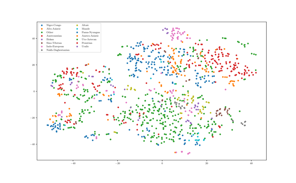
Figure 2: Visualisation of learned embeddings by family.

The visualization of the learned language embeddings projected to 2D via TSNE van der Maaten and Hinton (2008) can be seen in appendix in Figure 2. As we can see from the visualization, there are some clear clusters, however, further work would be needed to explain the clusters.

3.2.6 Development and Test Data

As in the Probabilistic system, we mix the visible part of the development data (and later test data) with the training data. This is needed in order to compute the language embeddings of the new languages.

3.3 The Combined System

We now describe the combination of the Probabilistic system and the Neural system which we submitted for evaluation within the shared task.

3.3.1 Analysis on Development Data

As will be shown in Table 1, both the Probabilistic system and the Neural system reach accuracies around 75% on the development data, with the Neural system being slightly better. However, a more detailed analysis showed that while the accuracies are similar, the errors the systems make are somewhat different: for 14% of the masked feature values in the development data, one of the systems predicts the correct value while the other system does not (in absolute numbers there are 225 such cases in the development data). An ensemble of the two systems could thus theoretically reach an accuracy of up to 82% if it were able to always select the correct prediction. This motivates our efforts in finding a way to combine the predictions of the two systems.

For this purpose, we utilize confidence scores produced by the two partial systems. For the Probabilistic system, its $score_{2}$ (Section 3.1.1) serves as the confidence score for each prediction; for the Neural system, we use the feature value probability produced by the last layer of the neural network.

We analyzed the confidence scores on the 225 predictions on development data where only one of the two systems predicted the correct feature value; in 48% of cases it was the Probabilistic system, in 52% it was the Neural system.

Unfortunately, we found neither of the confidence scores to be a very good predictor of the correctness of the prediction, with the Neural system confidence score being somewhat more reliable. Specifically, low confidence scores tend to indicate a potentially incorrect prediction for each of the systems: on the least confident quarter of the predictions (25% of the analyzed predictions with lowest confidence score), the accuracy was only around 40% for each of the systems. High confidence scores are only indicative for the Neural system (61% accuracy on the most confident quarter), for the Probabilistic system they seem to behave rather randomly (accuracy on the most confident quarter is only 44%.)

3.3.2 Submitted Solution

As the Neural system seems to perform better than the Probabilistic system, our final solution is to return the prediction of the Neural system as the final output, unless the Neural system confidence is very low and the Probabilistic system confidence is not too low. Specifically, if the Neural system confidence is below a threshold $T_{N}$ and the Probabilistic system confidence is above a threshold $T_{P}$, we return the prediction from the Probabilistic system, otherwise we return the prediction from the Neural system.

Based on the development data analysis, we found the optimal threshold values to be $T_{N}=0.65$ and $T_{P}=0.5$. On the development data, this leads to returning the output of the Probabilistic system instead of the Neural system in 6% of cases in which the predictions of the two systems differ, leading to an absolute gain of +1% in accuracy. On the test data, the output of the Probabilistic system was used in 10% of the differing cases.

3.4 Other Attempts

This section briefly describes some other approaches that we tried and abandoned because their accuracy was too low.

3.4.1 kNN

We used a simple kNN with Hamming distance to find the nearest neighbors of a language. The Hamming distance was calculated for each pair of languages as the number of features whose values in the two languages do not match. If one of the values for a given feature was unknown, we counted it as a mismatch. We then found $k$ nearest neighbors of each language and filled the required values using majority vote among the neighbors. This setup was able to achieve accuracy of 62.28% on development set using 22 nearest neighbors. We have also tried different fallbacks such as most common value of a feature overall, most common value in a genus or most common value in a family in case of not finding any value among the neighbors. However, we found out that these fallbacks had little to none impact on the final accuracy of the model.

3.4.2 Feed-forward Neural Network

We have also tried the classical feed-forward network to predict the required features. As input, we randomly masked some of the non-empty feature values. We then embedded each feature value into the embedding space and concatenated these feature embeddings into a single vector. After the concatenation layer, we added a few feed-forward layers and the classification head for each feature. We have tried various architectures and percentages of masked values with no success. We were able to achieve an accuracy of 56.45% on the development set, which is worse than the accuracy of kNN.

4 Evaluation

The evaluation metric is a simple accuracy: the number of correctly predicted feature values divided by the number of masked features. Failure to predict a value of a masked feature would count as an incorrect prediction. Nevertheless, our systems always predict all masked features, even if there are few reliable clues and the system’s confidence is low.

The accuracies of different setups are given in Table 1. The accuracy on the test data is the official number computed by the shared task organizers (Baseline and Combined) or by us using the official evaluation script (Probabilistic and Neural partial results); all the other results are computed on the development data. As a baseline, we evaluate a model where each feature receives its overall most probable value, regardless of language. Interestingly, the Probabilistic system outperforms the Neural system on the test data (contrary to what we observed on the development data) but the difference is again in the order of just a few wrong predictions.

System	Dev	Test
Baseline	53.45	51.39
Probabilistic	73.81	71.08
Neural	74.49	69.80
Combined	75.50	70.75
Feed-forward	56.45
kNN-Hamming	62.28
kNN-LangEmbed	68.10

Table 1: Accuracy of various models on the development and test data.

Accuracies computed on individual languages are skewed because for some languages the system had to predict only one feature. If we look at development languages where 10 or more features were masked, our Probabilistic system achieved 100% on four of them (Ukrainian, Uyghur, Wan and Venda); at the other end of the scale, accuracy on the South American language Uru is only 30%. The system never failed on 34 features; the most frequent of them is unsurprisingly (see Section 3.1) Minor morphological means of signaling negation, followed by Order of Relative Clause and Noun and Postnominal relative clauses. Note however that these observations do not necessarily indicate that a feature is easy or difficult to predict. The success depends heavily on how frequently the feature co-occurs with a suitable correlated feature in WALS, and whether our random masking selected the feature in presence or absence of the correlated feature.

5 Conclusion

We have described three systems (two individual systems and one combined system) that use the known features of a language to predict its remaining features. The first system is based on conditional probability of feature values, log frequency and mutual information. It achieves an accuracy of 73.81% on the development data. The second system uses a neural network to train language and feature embeddings, and to predict a feature value’s probability based on the embeddings. It achieves slightly better results than the probabilistic model on the development data, but it is slightly worse on the test data. Finally, we use the scores produced by the two systems together with their predictions to decide which of the systems knows the correct answer in which situation. This combined system achieves 75.50% on the development data and 70.75% on the test data.

Our code is available at https://github.com/ufal/ST2020.

Appendix A Appendix

References

- Bjerva et al. (2020) Johannes Bjerva, Elizabeth Salesky, Sabrina Mielke, Aditi Chaudhary, Giuseppe G. A. Celano, Edoardo M. Ponti, Ekaterina Vylomova, Ryan Cotterell, and Isabelle Augenstein. 2020. SIGTYP 2020 Shared Task: Prediction of Typological Features. In Proceedings of the Second Workshop on Computational Research in Linguistic Typology. Association for Computational Linguistics.
- Daumé III and Campbell (2007) Hal Daumé III and Lyle Campbell. 2007. A Bayesian model for discovering typological implications. In Proceedings of the 45th Annual Meeting of the Association for Computational Linguistics, pages 65–72, Praha, Czechia. Association for Computational Linguistics.
- Dryer and Haspelmath (2013) Matthew S Dryer and Martin Haspelmath. 2013. The World Atlas of Language Structures online.
- Greenberg (1963) Joseph H. Greenberg. 1963. Some universals of grammar with particular reference to the order of meaningful elements. In Joseph H. Greenberg, editor, Universals of Language, pages 110–113. MIT Press, London.
- Kingma and Ba (2014) Diederik P. Kingma and Jimmy Ba. 2014. Adam: A method for stochastic optimization. Cite arxiv:1412.6980Comment: Published as a conference paper at the 3rd International Conference for Learning Representations, San Diego, 2015.
- Le and Mikolov (2014) Quoc V. Le and Tomas Mikolov. 2014. Distributed representations of sentences and documents. CoRR, abs/1405.4053.
- van der Maaten and Hinton (2008) Laurens van der Maaten and Geoffrey Hinton. 2008. Visualizing data using t-SNE. Journal of Machine Learning Research, 9:2579–2605.
- O’Horan et al. (2016) Helen O’Horan, Yevgeni Berzak, Ivan Vulić, Roi Reichart, and Anna Korhonen. 2016. Survey on the use of typological information in natural language processing. In Proceedings of COLING 2016, the 26th International Conference on Computational Linguistics: Technical Papers, pages 1297–1308, Osaka, Japan. The COLING 2016 Organizing Committee.