Elementary Integral Series for Heun Functions

Abstract

Heun differential equations are the most general second order Fuchsian equations with four regular singularities. An explicit integral series representation of Heun functions involving only elementary integrands has hitherto been unknown and noted as an important open problem in a recent review. We provide explicit integral representations of the solutions of all equations of the Heun class: general, confluent, bi-confluent, doubly-confluent and triconfluent, with integrals involving only rational functions and exponential integrands. All the series are illustrated with concrete examples of use. These results stem from the technique of path-sums, which we use to evaluate the path-ordered exponential of a variable matrix chosen specifically to yield Heun functions. We demonstrate the utility of the integral series by providing the first representation of the solution to the Teukolsky radial equation governing the metric perturbations of rotating black holes that is convergent everywhere from the black hole horizon up to spatial infinity.

1 Introduction

The study of Heun equations has generated significant interest in both mathematics and physics lately. From a mathematical standpoint, recent results have uncovered relation between Heun equations other equations of paramount importance for physics. For example, it was found by means of antiquantisation procedures Slav1 and monodromy preserving transformations Takem1 that the Heun equations share a bijective relationship with Painlevé equations Slav1 ; Slav2 ; Slav4 . This permitted in-depth studies on the integral symmetry properties of equations of the Heun class Slav3 and to determine generating polynomial solutions of the Heun equation by formulating a Riemann-Hilbert problem for the Heun function RieHibH . The reduction of certain Heun equations under non-trivial substitutions to hypergeometric equations has also been possible by means of pull-back transformations based on Belyi coverings BelyiHeun and polynomial transformations Maier1 ; Maier2 .

In contrast, in spite of the increasing use of Heun functions in physics (in quantum optics Xie2010 ; Moham , condensed matter physics Crampe ; Dorey , quantum computing QuantComp , two-state problems QTS1 ; QTS2 and more Hort1 ), few studies Hort1 ; Hort2 have specifically focused on determining their properties most relevant to physical applications. For example, the lack of integral expansions of these functions involving only elementary integrands has been clearly identified as a major obstacle when extracting physical meaning from the mathematical treatment of black holes quasinormal modes Hort1 ; Hort2 , yet remains unaddressed in the mathematical literature. The present works tackles this issue by determining a novel integral representation of the Heun equations involving elementary functions that is tailored to physical applications. In particular, we demonstrate the applicability of the novel integral representation to the Teukolsky equation TeukEqn that governs the metric perturbations of rotating black holes and further explore which physical observables pertinent to black hole perturbation theory can be obtained from the integral form. The present progress in integral representation is enabled by the method of path-sum Giscard2015 , which generates the linear Volterra integral equation of the second kind satisfied by any function involved a system of coupled linear differential equations with variable coefficients.

This paper is organised as follows. In Section 2 we give the minimal necessary background on Heun equations. This section concludes in §2.4 with a review of existing integral representations of Heun functions and their major drawback as noted in the recent mathematical-physics literature. Section 3 is a self-contained presentation of the novel, elementary integral representations of all functions of Heun class, illustrated with concrete examples. This section contains none of the proofs, all of which are deferred to Appendix A. Then, in Section 4 we give the elementary integral series representation of the solution to the Teukolsky radial equation. This representation is the first one to be convergent from the black hole horizon up to spatial infinity. This stands in contrast to the state-of-the-art MST formalism Mano1997 , that uses two hypergeometric series (one convergent at the horizon and the other at infinity) that must then be matched after an analytic continuation procedure. This last step requires the introduction of an auxiliary parameter lacking physical correspondence, at the very least obscuring the physical picture. The convergence of the integral series over the entire domain from the black hole horizon up to spatial infinity therefore alleviates the need for such parameters lacking physical correspondence when calculating solutions of the Teukolsky radial equation. These solutions are of primary importance for computing quantities of physical interest such as gravitational wave fluxes Fujita2004 and quasinormal modes Zhang2013 . We conclude in §5 with a brief discussion of the novel integral series and future prospects of the method of path-sum from which they stem for solving the coupled system of Teukolsky angular and radial equations.

2 Heun Differential Equations

2.1 Mathematical Context

The most general linear, homogenous, second order differential equation with polynomial coefficients is given by the Fuchsian equation SpecFunc which has the following form

$$P(z)\frac{d^{2}y(z)}{dz^{2}}+Q(z)\frac{dy(z)}{dz}+R(z)y(z)=0,~{}z\in\mathbb{CP}^{1},$$

where $\mathbb{CP}^{1}$ is the Riemann sphere. In the above equation, if the function $K_{QP}=Q(z)/P(z)$ has a pole of at most first order and $K_{RP}=R(z)/P(z)$ has a pole of at most second order at some singularity $z=z_{0}$, then $z_{0}$ is called a Fuchsian singularity, otherwise it is an irregular singularity. The above equation is a Fuchsian equation if all its singularities are Fuchsian singularities. Now, any Fuchsian equation with exactly four singular points can be mapped onto a Heun equation HeunOrig by transformation in dependent or independent variables. These transformations are called s-homotopic and Möbius transformations respectively. The Heun equation is a straightforward generalisation of the hypergeometric equation, a Fuchsian equation with exactly three singular points SpecFunc .

2.2 General Heun Equation

As mentioned in the Introduction, the Heun differential equation is the most general Fuchsian equation with four regular singularities. The canonical form of the equation, also known as the General Heun Equation (GHE) is given by the following equation and conditions:

$$\frac{d^{2}y(z)}{dz^{2}}+\bigg{[}\frac{\gamma}{z}+\frac{\delta}{z-1}+\frac{\epsilon}{z-t}\bigg{]}\frac{dy(z)}{dz}+\frac{\alpha\beta z-q}{z(z-1)(z-t)}y(z)=0,$$ (1)

where $q\in\mathbb{C}$ is called the accessory parameter. The corresponding Riemann-P symbol is as follows:

$$\begin{pmatrix}0&1&a&\infty\\ 0&0&0&\alpha&;z\\ 1-\gamma&1-\delta&1-\epsilon&\beta\end{pmatrix}$$

where the parameters satisfy the Fuch’s condition:

$$1+\alpha+\beta=\gamma+\delta+\epsilon$$

The GHE has four singular points at $z=0,1,t,\infty$. Concerning its solutions, Maier, completing a task initiated by Heun Heun1888 himself has shown that solutions of the GHE have Coxeter group $D_{4}$ as their automorphism group Maier192 . This means that 192 solutions can be generated using the symmetries of $D_{4}$, much more than the 24 solutions of the Gauss Hypergeometric equation determined by Kummer Whittaker . We refer the reader to Maier192 for the complete list of solutions and their relations as well as to SpecFunc for a further discussion of their properties.

For specific parameter values the Heun equation reduces to other well-known equations of importance: e.g. setting $\epsilon=0,\gamma=\delta=1/2$ yields the Mathieu equation, which has found widespread applicability in the theoretical and experimental study of vibration phenomenon Mathieu ; Mathieu5 , electromagnetic scattering from elliptic waveguides Mathieu1 ; Mathieu2 ; Mathieu3 , ion traps in mass spectrometry Mathieu4 , stability of floating ships Mathieu6 . Furthermore, the confluent form of the Heun equation has found wide ranging applications in quantum particle confinement and interaction potentials ConfPot ; IntPot and in the Stark effect Slav5 ; SpecFunc .

2.3 Confluent Heun Equations

The GHE contains 4 regular singularities. If we apply a confluence procedure to two of its singularities such that we get an irregular singularity, we call the resultant equation a confluent Heun equation (CHE). The CHE contains at least one irregular singular point besides the regular singular points. We can construct local solutions in the vicinity of this irregular singular points by the means of (generally divergent) Thomé series SpecFunc . The number of parameters in the CHE are reduced by one. Thus by applying the confluence procedure laid out in SpecFunc to the singularities at $z=t$ and $z=\infty$ in equation 2, we get the CHE:

$$\frac{d^{2}y(z)}{dz^{2}}+\bigg{[}\frac{\gamma}{z}+\frac{\delta}{z-1}+\epsilon\bigg{]}\frac{dy(z)}{dz}+\frac{\alpha z-q}{z(z-1)}y(z)=0.$$ (2)

By continuing application of the confluence procedure, we obtain the bi-confluent Heun equation

$$\frac{d^{2}y(z)}{dz^{2}}+\bigg{[}\frac{\gamma}{z}+\delta+\epsilon z\bigg{]}\frac{dy(z)}{dz}+\frac{\alpha z-q}{z}y(z)=0,$$ (3)

and related doubly-confluent Heun equation

$$\frac{d^{2}y(z)}{dz^{2}}+\bigg{[}\frac{\delta}{z^{2}}+\frac{\gamma}{z}+1\bigg{]}\frac{dy(z)}{dz}+\frac{\alpha z-q}{z^{2}}y(z)=0,$$ (4)

as well as the triconfluent Heun equation

$$\frac{d^{2}y(z)}{dz^{2}}+\bigg{[}\gamma+\delta z+\epsilon z^{2}\bigg{]}\frac{dy(z)}{dz}+(\alpha z-q)y(z)=0.$$ (5)

We refer the reader to SpecFunc for further general informations on these functions.

2.4 Integral representations of Heun functions

Erdélyi was the first to give an integral equation relating the values taken at two points by a general Heun function Erdelyi . His equation, a Fredholm integral equation, involves an hypergeometric kernel and can be used to obtain a series representation of Heun functions as sums of hypergeometric functions with coefficients determined via recurrence relations. Applications of this result in the special cases of Mathieu and Lamé equations were discussed by Sleeman Sleeman . Naturally, since Erdélyi’s breakthrough many mathematical works on Heun equations were concerned with integral transformations involving Heun functions. In particular, based on the work of CarlitzCarlitz , Valent found an integral transform for the Heun equation in terms of Jacobi polynomials Valent ; Ishkhanyan gave expansions of the confluent Heun functions involving incomplete beta functions Ishkhanyan_2005 ; El Jaick and coworkers El_Jaick_2011 provided novel transformations and classified expansions for Heun functions involving hypergeometric kernels; and Takemura found an elliptic transformation relating Heun’s functions for different parameters based on the Weierstrass sigma function Takem2 . This brief list of contributions is far from exhaustive, we refer to the recent review Hort1 for more details.

The common feature of all of these integral transforms is that they contain higher transcendental functions which makes them physically opaque and of limited use for practical calculations. In addition, the resulting series representations for the Heun functions have insufficient radiuses of convergence Cook2016 causing difficulties for black hole perturbation theory (see Section LABEL:sec:5). These issues were noted in the recent review Hort1 on Heun’s functions, the current state of research on this being described as follows :

“No example has been given of a solution of Heun’s equation expressed in the form of a definite integral or contour integral involving only functions which are, in some sense, simpler.[…] This statement does not exclude the possibility of having an infinite series of integrals with ‘simpler’ integrands”.

In this work, we constructively prove the existence of such a representation for all types of Heun’s functions and for all parameters, in the form of infinite series of integrals whose integrands involve only rational functions and exponentials of polynomials. Furthermore, we show that the series converges everywhere except at the singular points of the Heun function. We show that any Heun function, general or (bi-, doubly-, tri-)confluent, is a sum of exactly two functions each of which satisfy a linear Volterra equation of the second kind with explicitely identified elementary kernels. In particular, any Heun function $H(z)$ itself satisfies a linear integral Volterra equation of the second kind with such an elementary kernel if either there is at least one non-singular point $z_{0}\in\mathbb{R}$ where $H(z_{0})=H^{\prime}(z_{0})$ or there is a point where $H(z_{0})=0$.

3 Elementary integral series for all types of Heun functions

Owing to the emphasis of the present work on concrete results and a physical application, all the technical mathematical proofs are deferred to Appendix A.

3.1 Notation

The $\ast$ notation is useful to denote iterated integrals. Let $K(z,z_{0})$ be a function of two variables that is continuous over $]z_{0},z[$. We denote $K(z,z_{0})=K^{\ast 1}(z,z_{0})$ and, for any integer $n>1$,

$$K^{\ast n}(z,z_{0})=\int_{z_{0}}^{z}K^{\ast(n-1)}(z,\zeta_{1})K(\zeta_{1},z_{0})d\zeta.$$

In other terms $K^{\ast n}$ is the Volterra composition Volterra1924 of $K$ with itself $n$-times. The only type of integral series that is required to present all results of this section is the following

$$G(z,z_{0}) :=\sum_{n=1}^{\infty}K^{\ast n}(z,z_{0}),$$

$$=K(z,z_{0})+\int_{z_{0}}^{z}K(z,\zeta_{1})K(\zeta_{1},z_{0})d\zeta_{1}$$

$$\hskip 14.22636pt+\int_{z_{0}}^{z}\int_{\zeta_{1}}^{z}K(z,\zeta_{2})K(\zeta_{2},\zeta_{1})K(\zeta_{1},z_{0})d\zeta_{2}d\zeta_{1}\,+\cdots,$$

see also Eq. (29). In the appendix, we show that once $z_{0}$ is fixed, the above series converges over any subinterval of $\mathbb{R}$ which does not contain a singularity of $K(z,z_{0})$. A bound on the convergence speed of the series is also provided.

The function $G(z,z_{0})$ defined above, is solution to the linear Volterra integral equation of the second kind

$$G(z,z_{0})=K(z,z_{0})+\int_{z_{0}}^{z}K(z,\zeta)G(\zeta,z_{0})d\zeta,$$ (6)

or, in $\ast$ notation, $G=K+K\ast G$. Thus, the function $G$ can either be evaluated from the integral series or by solving the above Volterra equation.

3.2 Results

We emphasize that all results stated remain valid for complex parameter values. This is crucial notably when forming solutions of the Teukolsky equation in the study of quasinormal modes, for which the frequency parameter takes complex values (see Eq. 21).

Corollary 1 (General Heun Equation).

Let $H_{G}(z)$ be solution of the General Heun Equation,

$$\frac{d^{2}H_{G}(z)}{dz^{2}}+\bigg{[}\frac{\gamma}{z}+\frac{\delta}{z-1}+\frac{\epsilon}{z-t}\bigg{]}\frac{dH_{G}(z)}{dz}+\frac{\alpha\beta z-q}{z(z-1)(z-t)}H_{G}(z)=0,$$

with initial conditions $H_{G}(z_{0})=H_{0}$ and $\dot{H}_{G}(z_{0})=H^{\prime}_{0}$, assuming that $z_{0}\in\mathbb{R}$ is not a singular point of $H_{G}$. Denote $I$ the largest real interval that contains $z_{0}$ and does not contain any singular point of $H_{G}$. Then, for any $z\in I$,

$$H_{G}(z) =H_{0}+H_{0}\int_{z_{0}}^{z}\!G_{1}(\zeta,z_{0})d\zeta+(H^{\prime}_{0}-H_{0})\left(\!e^{z-z_{0}}-1+\!\int_{z_{0}}^{z}\!(e^{z-\zeta}-1)G_{2}(\zeta,z_{0})d\zeta\right),$$

where $G_{i}=\sum_{n=1}^{\infty}K_{i}^{\ast n}$ and

$$K_{1}(z,z_{0}) =$$

$$1+e^{-z}\int_{z_{0}}^{z}\Big{\{}\frac{\zeta_{1}^{\gamma}(\zeta_{1}-1)^{\delta}(t-\zeta_{1})^{\epsilon}}{z^{\gamma}(z-1)^{\delta}(t-z)^{\epsilon}}e^{\zeta_{1}}\left(\frac{q-\alpha\beta\zeta_{1}}{\left(\zeta_{1}-1\right)\zeta_{1}\left(\zeta_{1}-t\right)}-\frac{\epsilon}{t-\zeta_{1}}-\frac{\gamma}{\zeta_{1}}-\frac{\delta}{\zeta_{1}-1}-1\right)\Big{\}}d\zeta_{1},$$

$$K_{2}(z,z_{0}) =\left(\frac{q-\alpha\beta z}{(z-1)z(z-t)}-\frac{\epsilon}{t-z}-\frac{\gamma}{z}-\frac{\delta}{z-1}-1\right)e^{z-z_{0}}-\frac{q-\alpha\beta z}{(z-1)z(z-t)}.$$

Example 1 (Elementary integral series converging to a general Heun function).

In order to illustrate concretely the above corollary, consider the following General Heun equation (here with arbitrary parameters),

$$\frac{d^{2}H_{G}(z)}{dz^{2}}+\bigg{[}\frac{2}{z}+\frac{7}{z-1}+\frac{(-1)}{z-4}\bigg{]}\frac{dH_{G}(z)}{dz}+\frac{(3/2)z-1}{z(z-1)(z-4)}H_{G}(z)=0,$$ (7)

with initial conditions $H_{G}(6)=H^{\prime}_{T}(6)=1$. Here, the largest real interval containing $6$ and none of the singular points $0$, $1$ and $t=4$ is $I=]4,+\infty[$. Thus Corollary 1 indicates that for any $z\in]4,+\infty[$,

$$H_{G}(z) =1+\int_{z_{0}}^{z}G_{1}(\zeta,z_{0})d\zeta,$$

$$=1+\sum_{n=1}^{\infty}\int_{6}^{z}K_{1}^{\ast n}(\zeta,6)d\zeta,$$

$$=1+\int_{6}^{z}K_{1}(\zeta,6)d\zeta+\int_{6}^{z}\int_{6}^{\zeta}K_{1}(\zeta,\zeta_{1})K_{1}(\zeta_{1},6)d\zeta_{1}d\zeta+\cdots,$$

with the kernel $K_{1}$ given by

$$K_{1}(z,z_{0}) =1-e^{-z}\frac{(z-4)}{z^{2}(z-1)^{7}}\int_{z_{0}}^{z}\!e^{\zeta_{1}}\frac{\zeta_{1}\left(\zeta_{1}-1\right)^{6}}{2\left(\zeta_{1}-4\right)^{2}}\left(2\zeta_{1}^{3}+10\zeta_{1}^{2}-67\zeta_{1}+14\right)d\zeta_{1}.$$

In Fig. (4), we show a purely numerical evaluation of $H_{G}(z)$ together with analytical estimates based on the first few orders of the above series, i.e. we give $H^{(m)}_{G}(z):=1+\sum_{n=1}^{m}\int_{6}^{z}K_{1}^{\ast n}(\zeta,6)d\zeta$, with $m=1,2,3$ and $m=6$. This exhibits the convergence of the Neumann series representation of the path-sum formulation of a general Heun function, as predicted by the theory.

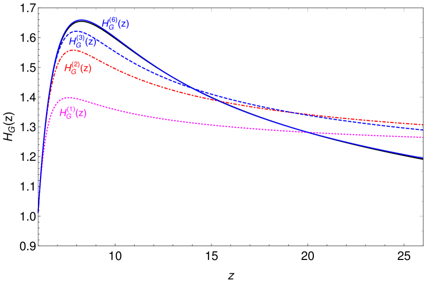
Figure 1: Convergence to a general Heun function with elementary integrals. Numerical evaluation of the general Heun function solution of Eq. (7) (solid black line), together with the first integral approximands of it: $H^{(1)}_{G}(z)$ (dotted magenta line), $H^{(2)}_{G}(z)$ (dot-dashed red line), $H^{(3)}_{G}(z)$ (dashed blue line) and $H^{(6)}_{G}(z)$ (solid blue line, very close to the numerical solution). For orders $m\geq 9$, we reach the numerical solution to within machine precision. Note that the integral series given here is convergent on $z\in]4,+\infty[$ but we show only the interval $z\in[6,26]$ for illustration purposes.

The results above continue to hold should e.g. $z_{0}=3$, in which case $I=]1,4[$; $z_{0}=1/2$ implying $I=]0,1[$; or $z_{0}=-20$ giving $I=]-\infty,0[$. In other terms, the integral representation given for the General Heun function is valid everywhere on $z\in\mathbb{R}\backslash\{0,1,t=4\}$ but can only be used in an interval $I$ where initial conditions for $H_{G}$ are available.

Corollary 2 (Confluent Heun Equation).

Let $H_{C}(z)$ be solution of the Confluent Heun Equation,

$$\frac{d^{2}H_{C}(z)}{dz^{2}}+\bigg{[}\frac{\gamma}{z}+\frac{\delta}{z-1}+\epsilon\bigg{]}\frac{dH_{C}(z)}{dz}+\frac{\alpha z-q}{z(z-1)}H_{C}(z)=0,$$

with initial conditions $H_{C}(z_{0})=H_{0}$ and $\dot{H}_{C}(z_{0})=H^{\prime}_{0}$, assuming that $z_{0}\neq 0$ and $z_{0}\neq 1$. If $z_{0}<0$, let $I=]-\infty,0[$, if $0<z_{0}<1$ let $I=]0,1[$, and else for $z_{0}>1$ let $I=]1,+\infty[$. Then, for any $z\in I$,

$$H_{C}(z) =H_{0}+H_{0}\int_{z_{0}}^{z}\!G_{1}(\zeta,z_{0})d\zeta+(H^{\prime}_{0}-H_{0})\left(\!e^{z-z_{0}}-1+\!\int_{z_{0}}^{z}\!(e^{z-\zeta}-1)G_{2}(\zeta,z_{0})d\zeta\right),$$

where $G_{i}=\sum_{n=1}^{\infty}K_{i}^{\ast n}$, $i=1,2$, and

$$K_{1}(z,z_{0}) =1+e^{-z}\int_{z_{0}}^{z}\Big{\{}\frac{e^{\zeta\epsilon}\zeta^{\gamma}\left(\zeta-1\right)^{\delta}}{e^{z\epsilon}z^{\gamma}(z-1)^{\delta}}e^{\zeta}\left(\frac{q-\alpha\zeta}{\left(\zeta-1\right)\zeta}-\frac{\gamma}{\zeta}-\frac{\delta}{\zeta-1}-\epsilon-1\right)\Big{\}}d\zeta,$$

$$K_{2}(z,z_{0}) =\left(\frac{q-\alpha z}{\left(z-1\right)z}-\frac{\gamma}{z}-\frac{\delta}{z-1}-\epsilon-1\right)e^{z-z_{0}}-\frac{q-\alpha z}{(z-1)z}.$$

Example 2 (Convergence to a Confluent Heun function).

Let us now consider the following Confluent Heun function $H_{C}(z)$ satisfying

$$\frac{d^{2}H_{C}(z)}{dz^{2}}+\bigg{[}\frac{3}{z}+\frac{(2/3)}{z-1}+4\bigg{]}\frac{dH_{C}(z)}{dz}+\frac{5z-1}{z(z-1)}H_{C}(z)=0$$ (8)

with initial conditions $H_{C}(-5)=0$ and $H^{\prime}_{C}(-5)=1$. Suppose that we wish to evaluate $H_{C}$ on the interval $z\in]-\infty,0[$, i.e. on both sides $z<z_{0}$ and $z>z_{0}$ of the conditions at $z_{0}=-5$. Then Corollary 2 indicates that, for any $z\in]-\infty,0[$, we have

$$H_{C}(z)=e^{z+5}-1+\int_{-5}^{z}(e^{z-\zeta}-1)G_{2}(\zeta,-5)d\zeta,$$

with $G_{2}=\sum_{n=1}^{\infty}K_{2}^{\ast n}$ and

$$K_{2}(z,z_{0})=\frac{3(5z-1)-e^{z-z_{0}}(3z+4)(5z-3)}{3(z-1)z}.$$

We emphasize that these results hold for all $z\in]-\infty,0[$ since this interval is divergence free, more precisely $K_{2}$ is bounded continuous on any compact subinterval of $]-\infty,0[$ and the integral series for $G_{2}$ is thus guaranteed to converge on this entire domain (this is shown in the appendix). Note that when considering $z<z_{0}$, all integrals remain the same as for $z>z_{0}$.

In Fig. (2) below, we show a purely numerical evaluation of $H_{C}(z)$ together with the truncated integral series approximations

$$H_{C}^{(m)}(z) :=\int_{-5}^{z}(e^{z-\zeta}-1)\Big{(}1+\sum_{n=1}^{m}K_{2}^{\ast n}(\zeta,-5)d\zeta\Big{)},$$ (9)

$$=\int_{-5}^{z}(e^{z-\zeta}-1)\Big{(}1+K_{2}(\zeta,-5)+\int_{-5}^{\zeta}K_{2}(\zeta,\zeta_{1})K_{2}(\zeta_{1},-5)d\zeta_{1}+\cdots\Big{)}.$$

Since kernel $K_{2}$ is singular at $z=0$ just as $H_{C}$ is, we expect the convergence speed of the integral series to slow down when approaching the singular point, as predicted by the bound of Eq.(30) presented in the appendix. This does not preclude analytically obtaining the correct asymptotic behavior for $H_{C}(z)$ as $z\to 0^{-}$. Indeed this follows from the behavior of $K_{2}$ under the same limit. We demonstrate such a procedure in §4.4.

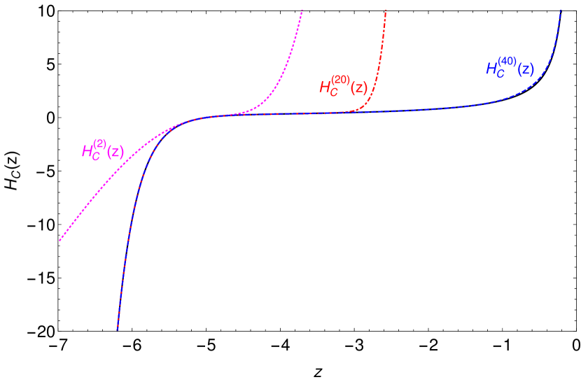
Figure 2: Convergence to a Confluent Heun function with elementary integrals over the interval $]-\infty,0[$. Numerical solution of the Eq. (8) (solid black line) with conditions $H_{C}(-5)=0$, $H_{C}^{\prime}(-5)=1$, together with its integral approximands as per Eq. (9), $H^{(2)}_{C}(z)$ (dotted magenta line), $H^{(20)}_{C}(z)$ (dot-dashed red line) and $H^{(40)}_{C}(z)$ (dashed blue line, very close to the numerical solution). Convergence near $z=0$ is slowed down due to $K_{2}$ being singular at $z=0$ just as $H_{C}$ is. Still, the integral series is convergent over the entire domain $z\in]-\infty,0[$, a crucial property for perturbative black hole theory that is unique to the present approach. Here as in subsequent examples we plot the various functions over smaller intervals for $z$, for illustration purposes.

Corollary 3 (Biconfluent Heun Equation).

Let $H_{B}(z)$ be solution of the Biconfluent Heun Equation,

$$\frac{d^{2}H_{B}(z)}{dz^{2}}+\bigg{[}\frac{\gamma}{z}+\delta+\epsilon z\bigg{]}\frac{dH_{B}(z)}{dz}+\frac{\alpha z-q}{z}H_{B}(z)=0,$$

with initial conditions $H_{B}(z_{0})=H_{0}$ and $\dot{H}_{B}(z_{0})=H^{\prime}_{0}$, assuming that $z_{0}\neq 0$. If $z_{0}>0$, denote $I=]0,+\infty[$ otherwise let $I=]-\infty,0[$. Then, for any $z\in I$,

$$H_{B}(z) =H_{0}+H_{0}\int_{z_{0}}^{z}\!G_{1}(\zeta,z_{0})d\zeta+(H^{\prime}_{0}-H_{0})\left(\!e^{z-z_{0}}-1+\!\int_{z_{0}}^{z}\!(e^{z-\zeta}-1)G_{2}(\zeta,z_{0})d\zeta\right),$$

where $G_{i}=\sum_{n=1}^{\infty}K_{i}^{\ast n}$, $i=1,2$, and

$$K_{1}(z,z_{0}) =1+e^{-z}\int_{z_{0}}^{z}\Big{\{}\frac{\zeta_{1}^{\gamma}}{z^{\gamma}}e^{\zeta_{1}-\frac{1}{2}\left(z-\zeta_{1}\right)\left(2\delta+\epsilon\left(\zeta_{1}+z\right)\right)}\Big{(}\frac{q-\alpha\zeta_{1}}{\zeta_{1}}-\frac{\gamma}{\zeta_{1}}-\delta-\zeta_{1}\epsilon-1\Big{)}\Big{\}}d\zeta_{1},$$

$$K_{2}(z,z_{0}) =\Big{(}\frac{q-\alpha z}{z}-\frac{\gamma}{z}-\delta-z\epsilon-1\Big{)}e^{z-z_{0}}-\frac{q-\alpha z}{z}.$$

Example 3 (Evaluating a Biconfluent Heun function via Volterra equations).

Let us now consider the following Biconfluent Heun function $H_{B}(z)$ satisfying

$$\frac{d^{2}H_{B}(z)}{dz^{2}}+\bigg{[}\frac{(1/10)}{z}+1+6z\bigg{]}\frac{dH_{B}(z)}{dz}+\frac{(-1)z-2}{z}H_{B}(z)=0,$$ (10)

with initial conditions $H_{B}(2/3)=0$ and $H^{\prime}_{B}(2/3)=-4$. Then Corollary 3 indicates that for $z>0$,

$$H_{B}(z) =2+2\int_{2/3}^{z}\!\!G_{1}(\zeta,2/3)d\zeta-6\left(\!e^{z-2/3}-1+\!\int_{2/3}^{z}\!(e^{z-\zeta}-1)G_{2}(\zeta,2/3)\!\right)d\zeta,$$ (11)

with $G_{i}=\sum_{n=1}^{\infty}K_{i}^{\ast n}$ for $i=1,2$, and

$$K_{1}(z,z_{0}) =1+\int_{z_{0}}^{z}\frac{(19-10\zeta(6\zeta+1))e^{-(z-\zeta)(3\zeta+3z+2)}}{10\zeta^{9/10}z^{1/10}}d\zeta,$$

$$K_{2}(z,z_{0}) =\frac{\big{(}19-10z(6z+1)\big{)}e^{z-z_{0}}-10(z+2)}{10z}.$$

Instead of evaluating functions $G_{1}$ and $G_{2}$ as the integral series, we may directly solve the linear integral Volterra equations that they satisfy, see Eq. (6). Such equations are very well behaved and numerically easy to solve, so that we can evaluate $H_{B}$ thanks to Eq. (11) with high numerical accuracy. In Fig. (3) below, we show the numerical evaluation of $H_{B}(z)$ obtained using a standard differential equations numerical solver versus the procedure described above.

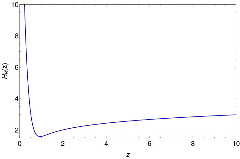
Figure 3: Biconfluent Heun function from Volterra equations. Numerical solution of the Eq. (8) (solid black line), together with the function predicted by Eq.(11) (dashed blue line). The two are indistinguishable. The integral representation of Eq. (11) is valid for $z\in]0,+\infty[$, we here show only $z\in]0,10[$ for illustration purposes.

Corollary 4 (Doubly-confluent Heun Equation).

Let $H_{D}(z)$ be solution of the Doubly-confluent Heun Equation,

$$\frac{d^{2}H_{D}(z)}{dz^{2}}+\bigg{[}\frac{\delta}{z^{2}}+\frac{\gamma}{z}+1\bigg{]}\frac{dH_{D}(z)}{dz}+\frac{\alpha z-q}{z^{2}}H_{D}(z)=0$$

with initial conditions $H_{D}(z_{0})=H_{0}$ and $\dot{H}_{D}(z_{0})=H^{\prime}_{0}$, assuming that $z_{0}\neq 0$. If $z_{0}>0$, denote $I=]0,+\infty[$ otherwise let $I=]-\infty,0[$. Then, for any $z\in I$,

$$H_{D}(z) =H_{0}+H_{0}\int_{z_{0}}^{z}\!G_{1}(\zeta,z_{0})d\zeta+(H^{\prime}_{0}-H_{0})\left(\!e^{z-z_{0}}-1+\!\int_{z_{0}}^{z}\!(e^{z-\zeta}-1)G_{2}(\zeta,z_{0})d\zeta\right),\,$$

where $G_{i}=\sum_{n=1}^{\infty}K_{i}^{\ast n}$, $i=1,2$, and

$$K_{1}(z,z_{0}) =1+e^{-z}\int_{z_{0}}^{z}\Big{\{}\frac{\zeta_{1}^{\gamma}}{z^{\gamma}}e^{-\frac{\delta}{\zeta_{1}}+2\zeta_{1}+\frac{\delta}{z}-z}\Big{(}\frac{q-\alpha\zeta_{1}}{\zeta_{1}^{2}}-\frac{\gamma}{\zeta_{1}}-\frac{\delta}{\zeta_{1}^{2}}-2\Big{)}\Big{\}}d\zeta_{1},$$

$$K_{2}(z,z_{0}) =\Big{(}\frac{q-\alpha z}{z^{2}}-\frac{\delta}{z^{2}}-\frac{\gamma}{z}-2\Big{)}e^{z-z_{0}}-\frac{q-\alpha z}{z^{2}}.$$

Example 4 (Convergence to a Doubly-Confluent Heun function).

Let us now consider the following Doubly-Confluent Heun equation, once again with arbitrarily chosen parameters for the example,

$$\frac{d^{2}H_{D}(z)}{dz^{2}}+\bigg{[}\frac{(-2)}{z^{2}}+\frac{1}{z}+1\bigg{]}\frac{dH_{D}(z)}{dz}+\frac{10z-(-1)}{z^{2}}H_{D}(z)=0$$ (12)

with initial conditions $H_{D}(1)=H^{\prime}_{D}(1)=1/2$. Then Corollary 4 indicates that for $z\in]0,+\infty[$,

$$H_{D}(z) =\frac{1}{2}+\frac{1}{2}\sum_{n=1}^{\infty}\int_{1}^{z}K_{1}^{\ast n}(\zeta,1)d\zeta,$$

with

$$K_{1}(z,z_{0})=1+\frac{e^{-z-\frac{1}{z}}}{z}\int_{z_{0}}^{z}e^{2\zeta_{1}+\frac{2}{\zeta_{1}}}\frac{1}{\zeta_{1}}(1-2\zeta_{1}^{2}+11\zeta_{1})d\zeta_{1}$$

In Fig. (4) below, we show a purely numerical evaluation of $H_{D}(z)$ together with analytical approximations based on the first few orders of the above series, i.e. we give $H_{D}^{(m)}(z):=1+\sum_{n=1}^{m}\int_{1}^{z}K_{1}^{\ast n}(\zeta,1)d\zeta$, with $m=3,5,8$. This demonstrates again the convergence of the Neumann series representation of the path-sum formulation of a general Heun function, as predicted by the theory. Here the exact $H_{D}(z)$ and $H_{D}^{(m)}(z)$ become indistinguishable for $m\geq 9$.

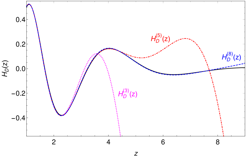
Figure 4: Convergence to Doubly-Confluent Heun function with elementary integrals. Numerical solution of the Eq. (12) (solid black line), together with its integral approximands $H^{(3)}_{D}(z)$ (dotted magenta line), $H^{(5)}_{D}(z)$ (dot-dashed red line) and $H^{(8)}_{D}(z)$ (dashed blue line). Note the integral series provided here is convergent for $z\in]0,+\infty[$ and show only the interval $z\in[1,9]$ for illustration purposes.

Corollary 5 (Triconfluent Heun Equation).

Let $H_{T}(z)$ be solution of the Triconfluent Heun Equation,

$$\frac{d^{2}H_{T}(z)}{dz^{2}}+\bigg{[}\gamma+\delta z+\epsilon z^{2}\bigg{]}\frac{dH_{T}(z)}{dz}+(\alpha z-q)H_{T}(z)=0,$$

with initial conditions $H_{T}(z_{0})=H_{0}$ and $\dot{H}_{T}(z_{0})=H^{\prime}_{0}$. Then, for any $z\in\mathbb{R}$,

$$y(z) =H_{0}+H_{0}\int_{z_{0}}^{z}\!G_{1}(\zeta,z_{0})d\zeta+(H^{\prime}_{0}-H_{0})\left(\!e^{z-z_{0}}-1+\!\int_{z_{0}}^{z}\!(e^{z-\zeta}-1)G_{2}(\zeta,z_{0})d\zeta\right),$$

where $G_{i}=\sum_{n=1}^{\infty}K_{i}^{\ast n}$, $i=1,2$ and

$$K_{1}(z,z_{0}) =1-e^{-\frac{1}{6}z\left(6\gamma+2z^{2}\epsilon+3\delta z+6\right)}\!\!\int_{z_{0}}^{z}\!\!e^{\frac{1}{6}\zeta\left(6\gamma+3\delta\zeta+2\zeta^{2}\epsilon+6\right)}\big{(}\zeta(\alpha+\delta+\zeta\epsilon)+\gamma-q+1\big{)}d\zeta,$$

$$K_{2}(z,z_{0}) =-\big{(}\epsilon z^{2}+(\alpha+\delta)z-q+\gamma+1\big{)}e^{z-z_{0}}-(q-z\alpha).$$

Example 5 (Convergence to a complex-valued Triconfluent Heun function).

Consider the Triconfluent Heun function defined as the solution to

$$\frac{d^{2}H_{T}(z)}{dz^{2}}+\bigg{[}2-z+7z^{2}\bigg{]}\frac{dH_{T}(z)}{dz}+(z-(2+i))H_{T}(z)=0,$$ (13)

where $i^{2}=-1$, and with initial conditions $H_{T}(-5)=H^{\prime}_{T}(-5)=2$. Corollary 5 indicates that for $z\in\mathbb{R}$,

$$H_{D}(z) =2+2\int_{z_{0}}^{z}G_{1}(\zeta,-10)d\zeta,$$

with $G_{1}=\sum_{n=1}^{\infty}K_{1}^{\ast n}$ and

$$K_{1}(z,z_{0})=1-e^{\frac{1}{6}(3-14z)z^{2}-3z}\int_{z_{0}}^{z}e^{-\frac{1}{6}(3-14\zeta)\zeta^{2}+3\zeta}(7\zeta^{2}+1-i)\,d\zeta.$$

We show in Fig. (5) convergence to the complex-valued triconfluent Heun function by the integral series

$$H_{T}^{(m)}(z) :=2+2\int_{z_{0}}^{z}\sum_{n=1}^{m}K^{\ast n}_{1}(\zeta,-10)d\zeta,$$

$$=2+2\int_{z_{0}}^{z}K_{1}(\zeta,-10)d\zeta+\int_{z_{0}}^{z}\int_{z_{0}}^{z}K_{1}(z,\zeta_{1})K_{1}(\zeta_{1},-10)d\zeta_{1}d\zeta+\cdots$$

With this example, we emphasize that all the integrals representations obtained here remain valid for complex-valued Heun functions.

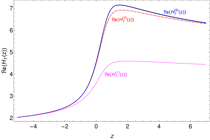
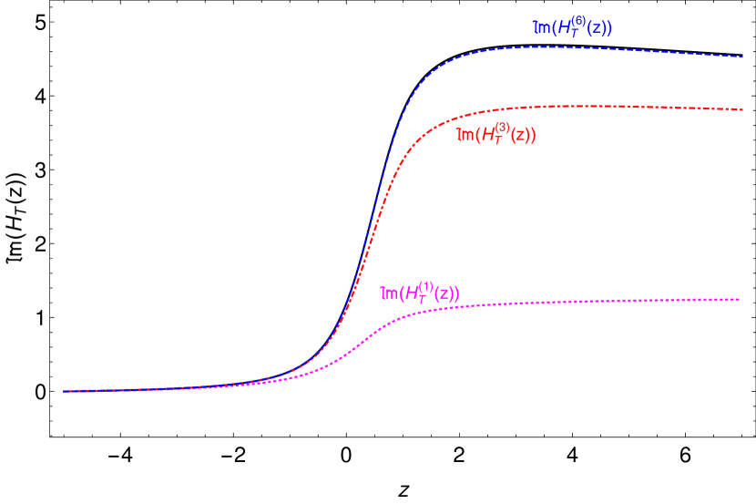
Figure 5: Convergence to a complex-valued Triconfluent Heun function with elementary integrals. Numerical solution of the Eq. (13) (solid black line), together with its integral approximands $H^{(1)}_{T}(z)$ (dotted magenta line), $H^{(3)}_{T}(z)$ (dot-dashed red line) and $H^{(6)}_{T}(z)$ (dashed blue line). Top figure: real parts of these quantities. Bottom figure: imaginary parts of these quantities. Note that the integral series provided is convergent over the entire real line, we here show only the interval $z\in[-5,7]$ for illustration purposes.

Having focused on concrete evaluations of various Heun functions in the illustrative examples, we now turn to using the elementary integral series in the field of black hole physics.

4 Application to Black-Hole Perturbation Theory

4.1 Motivations

The theory of metric perturbations of Kerr black holes is governed by the Teukolsky equation TeukEqn . This equation provides the basic mathematical framework to study the stability of Schwarzschild Finster2009 and Kerr black holes Costa2020 and yields physical insights in the broader field of gravitational wave astrophysics Sasaki2003 . With the advent of event detections by LIGO LIGO2016 ; LIGO2020 , obtaining a better analytical grasp over the solutions of the Teukolsky equation is paramount in modeling the ringdown stage London2014 of a binary black hole merger using accurate waveform templates McWilliams2019 .

In the frequency domain, the Teukolsky equation can be decoupled into radial and angular components TeukEqn . Determining the analytical solutions of the radial equation has been an active area of research since the first formulation of the equations Mano1996 ; Sasaki2003 . To this end, state-of-the-art approaches all rely on the same strategy: i) obtain two series expansions of the solution, one convergent near the black hole horizon the other at spatial infinity; and ii) match both expansions at some intermediate radial point. The standard implementation of this strategy, due to Mano, Suzuki and Takasugi (MST) Mano1996 ; Mano1997 , relies on a series of hypergeometric functions at the black hole horizon and of Coulomb wave functions at spatial infinity. Matching both expansions requires the introduction of an auxiliary parameter $\nu$. We stress that this parameter is not part of the original parameters of the Teukolsky equation. Rather $\nu$ is a mathematical checkpost introduced to establish the convergence and matching of the hypergeometric and Coulomb series Fujita2004 . The MST strategy successfully yields accurate numerical data for studying gravitational wave radiation from Kerr black holes Sasaki2003 ; Fujita2004 . It is “the only existing method that can be used to calculate the gravitational waves emitted to infinity to an arbitrarily high post-Newtonian order in principle.” Sasaki2003 . At the same time, it has been explicitly recognised that the mathematical complexity of the formalism obscures physical insights into the problem Sasaki2003 . In particular, the auxiliary parameter $\nu$, which has been called ”renormalised angular momentum” to make it more palatable, has limited correspondence to physical phenomenon, if any.

More recently, explicit, analytic solutions to the Teukolsky equation have been established in terms of Heun functions Fiziev2 . Yet, Cook and Zalutskiy Cook1 note that in order to extract physical quantities of interest out of this approach, one is forced to revert to Leaver’s formalism Leaver1985 because “the series solution around z = 1 has a radius of convergence no larger than 1, far short of infinity”. Thus, just as for the MST formalism the problem is, in essence, that we are lacking a single representation of the solution to the Teukolsky radial equation that is convergent from the black hole horizon up to spatial infinity. The integral series provided in this work addresses this issue completely since it converges on this entire domain, thereby retaining the crucial features of the MST formalism that lead to its widespread applicability, while also not requiring any auxiliary, unphysical parameter. In a similar vein, we can assert that our formalism is suited for practical numerical and even analytical, calculations since the integral series are rapidly convergent, and their asymptotic behavior is analytically available. We may therefore also hope that the integral series representation will help solve the well-recognised computational difficulties that emerge from the MST formalism when applied to gravitational wave physics, in particular for the two body problem Bini2013 , and in the gravitational self force program Sago2003 ; Hikida2004 ; Kavanagh2016 .

For completeness, we begin with a brief discussion of the theory of the Teukolsky equation and its reduction to Heun form. We then give the series representation of its solution. Finally, we establish its asymptotics at both the black hole horizon ($z\to 1^{+}$) and spatial infinity ($z\to+\infty$).

4.2 The Teukolsky Equation : background

The Teukolsky Equation TeukEqn is a gauge invariant equation GaugeInv that governs the curvature perturbations of the Kerr black hole MWT . By making use of the Newman-Penrose formalism NewmanPenrose , the single master equation for the spin $(s)$ weighted scalar wave function ${}_{s}\psi$ in Boyer-Lindquist co-ordinates $\{t,r,\theta,\phi\}$ BoyerLindquist and the Kinnersley tetrad Kintetrad is written as:

$$\bigg{[}\frac{(r^{2}+a^{2})^{2}}{\Delta}-a^{2}\sin^{2}\theta\bigg{]}\frac{\partial^{2}_{s}\psi}{\partial t^{2}}+\bigg{(}\frac{4Mar}{\Delta}\bigg{)}\frac{\partial^{2}_{s}\psi}{\partial t\partial\phi}+\bigg{[}\frac{a^{2}}{\Delta}-\frac{1}{sin^{2}\theta}\bigg{]}\frac{\partial^{2}_{s}\psi}{\partial\phi^{2}}$$

$$-\Delta^{-s}\frac{\partial}{\partial r}\bigg{(}\Delta^{s+1}\frac{\partial_{s}\psi}{\partial r}\bigg{)}-\frac{1}{\sin\theta}\frac{\partial}{\partial\theta}\bigg{(}\sin\theta\frac{\partial_{s}\psi}{\partial\theta}\bigg{)}-2s\bigg{[}\frac{a(r-M)}{\Delta}+\frac{i\cos\theta}{\sin^{2}\theta}\bigg{]}\frac{\partial_{s}\psi}{\partial\phi}$$

$$-2s\bigg{[}\frac{M(r^{2}-a^{2})}{\Delta}-r-ia\cos\theta\bigg{]}\frac{\partial}{\partial t}+(s^{2}\cot^{2}\theta-s)_{s}\psi=4\pi\Sigma T$$ (14)

where the auxiliary variables are given by:

$$\Sigma\equiv r^{2}+a^{2}\cos^{2}\theta,\Delta\equiv r^{2}-2Mr+a^{2}$$ (15)

Here, $M$ is the mass of the black hole, $a$ is its angular momentum (per unit mass), $T$ is the source term built from the energy-momentum tensor TeukEqn and the spin parameter $s=0,\pm 1/2,\pm 1,\pm 2\pm 3/2$ for scalar, neutrino, electromagnetic, gravitational and Rarita-Schwinger RaritaSchwinger fields respectively. It reduces to the Bardeen-Press equation BardeenPress in the non-rotating $(a=0)$ case.

The equation 14 can be separated in time Krivan1997 and frequency domain TeukEqn . The latter can be performed for the vacuum case $(T=0)$ by the following separation ansatz:

$${}_{s}\psi(t,r,\theta,\phi)=e^{-i\omega t}e^{im\phi}S(\theta)R(r).$$ (16)

For the radial function $R(r)$ we obtain the Teukolsky Radial Equation (TRE):

$$\Delta^{-s}\frac{d}{dr}\bigg{[}\Delta^{s+1}\frac{dR(r)}{dr}\bigg{]}+\bigg{[}\frac{K^{2}-2is(r-M)K}{\Delta}+4is\omega r-\lambda\bigg{]}R(r)=0,$$ (17)

where,

$$K\equiv(r^{2}+a^{2})\omega-am,\quad\lambda\equiv\,_{s}A_{lm}(a\omega)+a^{2}\omega^{2}-2am\omega.$$ (18)

For the angular equation, we make $x\equiv\cos\theta$. Now the function $S(\theta)=\,_{s}S_{lm}(x;a\omega)$ is the spin weighted spheroidal function Breuer1977 which gives the solution for the Teukolsky Angular Equation (TAE):

$$\partial_{x}\bigg{[}(1-x^{2})\partial_{x}[_{s}S_{lm}(x;c)]\bigg{]}+\bigg{[}(cx)^{2}-2csx+s$$ (19)

$$\hskip 99.58464pt+\,_{s}A_{lm}(c)-\frac{(m+sc)^{2}}{1-x^{2}}\bigg{]}\,_{s}S_{lm}(x;c)=0,$$

where $c=a\omega$ is the oblateness parameter, $m$ is the azimuthal separation constant and ${}_{s}A_{lm}(c)$ is the angular separation constant. The equations 17 and 19 are coupled equations which require simultaneous evaluation of the parameters $\omega$ and ${}_{s}A_{lm}(c)$. Given a value for ${}_{s}A_{lm}(c)$, we can solve 17 for the complex frequency $\omega$ and given the latter, we can solve 19 as an eigenvalue problem for ${}_{s}A_{lm}(c)$.

4.3 Teukolsky Radial Equation in Heun Form

We now reduce the Teukolsky Radial Equation to the non-symmetrical Heun form, which allows us to represent its solution with the results of Section. 3. There is one small consideration to be noted: depending on the sign of the spin $s$ we wish to operate in, certain parameters of the CHE form of the TAE and TRE flip their signs as given in Fiziev2 . However this is not of relevance for our purposes since our main aim is to work with the CHE form of the equations that obviously remains irrespective of the sign of the spin parameter.

The radial function $R(r)$ solution to Eq. 17 has three singularities: an irregular singular point at $r=\infty$ and two regular singular points corresponding to the roots of $\Delta=0$, which are

$$r_{\pm}=M\pm\sqrt{M^{2}-a^{2}}$$

The values $r_{\pm}$ correspond to the event and Cauchy horizon respectively (for an in-depth introduction to the notation and terminology on back-hole mathematics, we refer the reader to MWT ). Having identified these, we may now map the Teukolsky Radial Equation into an Heun equation. We close following the standard treatment Cook1 . We begin by letting the radial function $R$ be of the form

$$R(r)=(r-r_{+})^{\xi}(r-r_{-})^{\eta}e^{\zeta r}H(r),$$ (20)

where the parameters $\zeta,\xi,\eta$ are given by

$$\zeta=\pm i\omega\equiv\zeta_{\pm},\qquad\xi=\frac{-2\pm(s+2i\sigma_{+})}{2}\equiv\xi_{\pm},$$ (21)

$$\eta=\frac{-s\pm(s-2i\sigma_{-})}{2}\equiv\eta_{\pm},\qquad\sigma_{\pm}=\frac{2\omega Mr_{\pm}-ma}{r_{+}-r_{-}}.$$

With the dimensionless variables

$$\bar{r}\equiv\frac{r}{M},\quad\bar{a}\equiv\frac{a}{M},\quad\bar{\omega}\equiv M\omega,\quad\bar{\zeta}\equiv M\zeta,$$

we transform the radial coordinate $r$ into the dimensionless variable $z$ defined by

$$z=\frac{r-r_{-}}{r_{+}-r_{-}}=\frac{\bar{r}-\bar{r}_{-}}{\bar{r}_{+}-\bar{r}_{-}}$$

Now, any of the eight possible combinations of the parameters $\{\zeta,\xi,\eta\}$ given in Eqs. (21) will reduce the Teukolsky Radial Equation (17) into the following equation for the auxiliary function $H$,

$$\frac{d^{2}H(z)}{dz^{2}}+\Bigg{(}\frac{\gamma}{z}+\frac{\delta}{z-1}+4p\Bigg{)}\frac{dH(z)}{dz}+\frac{4\alpha pz-\sigma}{z(z-1)}H(z)=0$$ (22)

which is a Confluent Heun equation. Here, the following variables have been introduced to clarify the equation,

$$p=(\bar{r}_{+}-\bar{r}_{-})\frac{\bar{\zeta}}{2},\qquad\alpha=1+s+\xi+\eta-2\bar{\zeta}+s\frac{i\bar{\omega}}{\bar{\zeta}},$$ (23)

$$\gamma=1+s+2\eta,\qquad\delta=1+s+2\xi,$$

$$\sigma=\,_{s}A_{lm}(\bar{a}\bar{\omega})+\bar{a}^{2}\bar{\omega}^{2}-8\bar{\omega}^{2}+p(2\alpha+\gamma-\delta)+\bigg{(}1+s-\frac{\gamma+\delta}{2}\bigg{)}\bigg{(}s+\frac{\gamma+\delta}{2}\bigg{)}.$$

Furthermore, the local solutions at the singularities have the exact same form for all eight combinations of the parameters $\{\zeta,\xi,\eta\}$ given in Eqs. (21). More precisely, we get

$$\lim_{z\to 0}R(z)\sim z^{-s+i\sigma_{-}}\quad\text{or}\quad z^{-i\sigma_{-}},$$ (24a)

$$\lim_{z\to 1}R(z)\sim(z-1)^{-s-i\sigma_{+}}\quad\text{or}\quad(z-1)^{i\sigma_{+}},$$ (24b)

$$\lim_{z\to\infty}R(z)\sim z^{-1-2s+2i\bar{\omega}}e^{i(\bar{r}_{+}-\bar{r}_{-})\bar{\omega}z}\quad\text{or}\quad z^{-1-2i\bar{\omega}}e^{-i(\bar{r}_{+}-\bar{r}_{-})\bar{\omega}z}$$ (24c)

Now, the above forms correspond to behaviour of the perturbations at the boundary conditions of the event and Cauchy horizon and spatial infinity. By suitable choice of the signs in 24a,  24b and 24c, we can obtain expressions for quantities of physical interest such as Quasinormal Modes and Totally Transmitting Modes Cook1 . Also, see Navaes2019 ; Suzuki1998 ; Suzuki1999 ; Yoshida2010 for applications of the Heun form of the Teukolsky equations. The equation can be solved by various methods such as Frobenius series about the singular points Fiziev2 and continued fractions Leaver1985 .

4.4 Representation of the Teukolsky radial function convergent on $]1,+\infty[$

4.4.1 Elementary integral series

The solution of the Confluent Heun equation (22) satisfied by the auxiliary function $H(z)$ is described by Corollary (2). Since the singular points are located at $z=0,1,+\infty$, given any initial conditions for $H(z_{0})$ and $\dot{H}(z_{0})$ at $z_{0}\in]1,+\infty[$, the integral series representation of $H(z)$ is guaranteed to converge on the entire domain $]1,+\infty[$. This crucial property stands in stark contrast with the hypergeometric and Coulomb series, which converge close to 1 and to $+\infty$, respectively. Because of this, we do not need to introduce the unphysical parameter $\nu$.

Recall that the Teukolsky radial function $R$ and auxiliary function $H$ are related by Eq. (20). The auxiliary function is a confluent Heun function given by the following integral series representation, convergent for any $z\in]1,+\infty[$,

$$H(z) =H_{0}+H_{0}\int_{z_{0}}^{z}G_{1}(\zeta,z_{0})d\zeta+(H^{\prime}_{0}-H_{0})\!\left(\!e^{z-z_{0}}-1\!+\!\int_{z_{0}}^{z}\!\!(e^{z-\zeta}-1)G_{2}(\zeta,z_{0})d\zeta\right)\!,$$

where $G_{i}=\sum_{n=1}^{\infty}K_{i}^{\ast n}$, $i=1,2$, and

$$K_{1}(z,z_{0}) =1+e^{-(1+4p)z}z^{-\gamma}(z-1)^{-\delta}\times$$

$$\hskip 14.22636pt\int_{z_{0}}^{z}\Big{\{}e^{(1+4p)\zeta}\zeta^{\gamma}\left(\zeta-1\right)^{\delta}\left(\frac{\sigma-4\alpha p\zeta}{\left(\zeta-1\right)\zeta}-\frac{\gamma}{\zeta}-\frac{\delta}{\zeta-1}-4p-1\right)\Big{\}}d\zeta,$$

$$K_{2}(z,z_{0}) =\left(\frac{\sigma-4\alpha pz}{\left(z-1\right)z}-\frac{\gamma}{z}-\frac{\delta}{z-1}-4p-1\right)e^{z-z_{0}}-\frac{\sigma-4\alpha pz}{(z-1)z}.$$

Here we assumed $z_{0}\in]1,+\infty[$ then $H_{0}:=H(z_{0})$, $H^{\prime}_{0}:=\dot{H}(z_{0})$ and all parameters are given by Eq. (23).

Witnessing to the fact that the above representation is convergent for all $z\in]1,+\infty[$, we here recover the asymptotic behavior of $H(z)$ in both limits $z\to 1^{+}$ and $z\to+\infty$. We emphasize that this is not possible with any single series representation of $H(z)$, which converges either in the vicinity of $1^{+}$ or of $+\infty$.

4.4.2 Asymptotic behavior for $z\to+\infty$

From now on, we write $F(z)\sim_{a.e.}$ to present the leading term of the asymptotic expansion of the function $F(z)$, disregarding constant factors. For example, we would write $1+2/z\sim_{a.e}z^{-1}$ as $z\to 0$.

We begin by determining the asymptotic behavior of $K_{1}(z,z_{0})$ for $z\gg 1$. This depends on two cases: $p=0$ and $p\neq 0$. We suppose first that $p=0$ and assume that $\delta+\gamma>0$. In this situation, the confluent Heun function becomes a well understood hypergeometric function Erdelyi1955 ; Motygin2018OnEO for which we will nonetheless show that we recover the correct asymptotic behavior. Setting $p=0$ we get, as $z\to+\infty$,

$$K_{1}(z,z_{0}) \sim_{a.e}1+e^{-(1+4p)z}z^{-\gamma}(z-1)^{-\delta}\left(-e^{z}z^{\gamma+\delta}+e^{z_{0}}z_{0}^{\gamma+\delta}\right),$$

$$\sim_{a.e}e^{-z}z^{-\delta-\gamma}e^{z_{0}}z_{0}^{\gamma+\delta}.$$

Then $K_{1}(z,z_{0})$ is asymptotically the product of a function depending only on $z$ and of a function depending only on $z_{0}$. This property is sufficient to determine the asymptotic behavior of $G_{1}$ in closed-form

$$G_{1}(z,z_{0})\sim_{a.e}e^{-z}z^{-\delta-\gamma}e^{z_{0}}z_{0}^{\gamma+\delta}e^{\int_{z_{0}}^{z}e^{-\zeta}\zeta^{-\delta-\gamma}e^{\zeta}\zeta^{\gamma+\delta}d\zeta}=(z_{0}/z)^{\delta+\gamma}$$

implying that $\int_{z_{0}}^{z}G_{1}(\zeta,z_{0})d\zeta\sim_{a.e.}z^{1-\delta-\gamma}$ for $z\to+\infty$. Analyzing $K_{2}$ and $G_{2}$ yields the same results. Indeed, with $p=0$, we have

$$K_{2}(z,z_{0})\sim_{a.e.}\left(\frac{-1}{z}(\gamma+\delta)-1\right)e^{z-z_{0}},$$

which is the product of a function of $z$ and a function $z_{0}$ so we determine

$$G_{2}(z,z_{0})\sim_{a.e.}\left(\frac{-1}{z}(\gamma+\delta)-1\right)e^{z-z_{0}}e^{-(z-z_{0})}(z_{0}/z)^{\gamma+\delta},$$

that is $G_{2}\sim_{a.e.}z^{-\gamma-\delta}$. From there $e^{z-z_{0}}-1\!+\!\int_{z_{0}}^{z}\!\!(e^{z-\zeta}-1)G_{2}(\zeta,z_{0})d\zeta\sim_{a.e.}z^{1-\gamma-\delta}$. Thus for $p=0$ and $\delta+\gamma>0$, we get $H(z)\sim_{a.e.}z^{1-\delta-\gamma}$ regardless of the conditions at $z_{0}$ and provided $\delta+\gamma>0$, as expected Erdelyi1955 . Further cases arise for $\delta+\gamma\leq 0$ but we do not discuss these here as they correspond to well known hypergeometric results.

Let us now suppose that $p\neq 0$. Then, since

$$e^{4p\zeta}\zeta^{\gamma}\left(\zeta-1\right)^{\delta}f(\zeta)=-e^{4p\zeta}\zeta^{\gamma+\delta}\left(\frac{4\alpha p+\gamma+\delta}{\zeta}+4p+O(1/\zeta^{2})\right),$$

we have, asymptotically for $z\to+\infty$,

$$K_{1}(z,z_{0})\sim_{a.e.}1-e^{-4pz}z^{-\gamma}z^{-\delta}\times z^{\gamma+\delta}\left(e^{4pz}-4\alpha p\,E_{-\gamma-\delta+1}(-4pz)\right).$$

where $E_{n}(z)$ is the exponential integral function, with asymptotic expansion $E_{n}(x)\sim_{a.e.}e^{-x}/x$ as $x\to+\infty$. This result greatly simplifies $K_{1}$, reducing it to

$$K_{1}(z,z_{0})\sim_{a.e}-\frac{\alpha}{z},\text{ as }z\to+\infty.$$

This allows us to determine the asymptotic behavior of $G_{1}$ straightforwardly as

$$G_{1}(z,z_{0})\sim_{a.e}\frac{-\alpha}{z}e^{\int_{z_{0}}^{z}-\alpha/\zeta\,d\zeta}=-\alpha z^{-1-\alpha},$$

and therefore $\int_{z_{0}}^{z}G_{1}(\zeta,z_{0})d\zeta\sim_{a.e.}z^{-\alpha}$ for $z\to+\infty$.

We proceed similarly for $K_{2}$ and $G_{2}$. We have $K_{2}(z,z_{0})=f(z)e^{z-z_{0}}+O(1/z),$ so that asymptotically $K_{2}(z,z_{0})\sim_{a.e.}f(z)e^{z}e^{-z_{0}}$ for $z\to+\infty$. Then $K_{2}(z,z_{0})$ is asymptotically the product of a function depending only on $z$ and of a function depending only on $z_{0}$. We therefore obtain

$$G_{2}(z,z_{0})\sim_{a.e.}e^{z-z_{0}}f(z)e^{\int_{z_{0}}^{z}f(\zeta)d\zeta},\text{ as }z\to+\infty.$$

The right hand-side is

$$e^{z-z_{0}}f(z)e^{\int_{z_{0}}^{z}f(\zeta)d\zeta} =e^{-4p(z-z_{0})}\left(\frac{z_{0}-1}{z-1}\right)^{\delta}\left(\frac{z_{0}}{z}\right)^{\gamma+\sigma}\left(\frac{1-z_{0}}{1-z}\right)^{4\alpha p-\sigma}$$

$$\times\frac{1}{z(z-1)}(\gamma-z(\gamma+\delta+4p(\alpha+z-1)+z-1)+\sigma)$$

which yields the asymptotic result,

$$G_{2}(z,z_{0})\sim_{a.e.}e^{-4pz}z^{-\delta-\gamma-4\alpha p},\text{ as }z\to+\infty.$$

This implies that

$$\left(\!e^{z-z_{0}}-1\!+\!\int_{z_{0}}^{z}\!\!(e^{z-\zeta}-1)G_{2}(\zeta,z_{0})d\zeta\right)\sim_{a.e.}e^{-4pz}z^{-4\alpha p-\delta-\gamma}.$$

Gathering our results, we conclude that when $p\neq 0$,

$$H(z)\sim_{a.e.}z^{-\alpha}~{}~{}~{}\text{or}~{}~{}~{}H(z)\sim_{a.e.}e^{-4pz}z^{-4\alpha p-\delta-\gamma},~{}\text{ as }z\to+\infty,$$

which gives the same asymptotic behavior as obtained from series designed to converge when $z\to+\infty$ Motygin2018OnEO ; Cook1 ; Ronveaux1995 . The result for $p=0$ yields the correct asymptotics of the hypergeometric function obtained in this case.

4.4.3 Asymptotic behavior for $z\to 1^{+}$

In this situation, we begin with

$$K_{1}(z,z_{0}) \sim_{a.e}1+e^{-(1+4p)z}(z-1)^{-\delta}\int_{z_{0}}^{z}\Big{\{}e^{(1+4p)\zeta}\left(\zeta-1\right)^{\delta-1}\left(c+c^{\prime}(\zeta-1)\right)\Big{\}}d\zeta,$$

where $c=\sigma-4\alpha p-\delta$ and $c^{\prime}=\gamma+4p+1$. In order to progress without presenting cumbersome equations, denote $F(\zeta)$ the following indefinite integral

$$F_{\delta}(\zeta): =\int e^{(1+4p)\zeta}\left(\zeta-1\right)^{\delta}d\zeta,$$

$$=-e^{4p+1}(\zeta-1)^{\delta+1}E_{-\delta}\big{(}-(1+4p)(\zeta-1)\big{)},$$

where $E_{n}(x)$ is the exponential integral function. In particular $E_{n}(x)\sim_{a.e.}x^{n-1}c_{1}+c_{2}$ as $x\to 0^{+}$ and where $c_{1}$ and $c_{2}$ are non-zero real constants that are irrelevant here. This implies $F_{\delta}(\zeta)\sim_{a.e.}(\zeta-1)^{1+\delta}$. Now given that

$$K_{1}(z,z_{0})=1+e^{-(1+4p)z}(z-1)^{-\delta}\big{(}cF_{\delta-1}(z)-cF_{\delta-1}(z_{0})+c^{\prime}F_{\delta}(z)-c^{\prime}F_{\delta}(z_{0})\big{)}.$$

then

$$K_{1}(z,z_{0})\sim_{a.e.}1,\text{ as }z\to 1^{+}.$$

This implies that $G_{1}(z,z_{0})\sim_{a.e}e^{z-z_{0}}$ and therefore $\int_{z_{0}}^{z}G_{1}(\zeta,z_{0})d\zeta\sim_{a.e.}1$ as $z\to 1^{+}$.

For $K_{2}$ and $G_{2}$ we begin by noting that for $z$ close to 1,

$$K_{2}(z,z_{0})\sim_{a.e.}\frac{4\alpha p}{z-1}(1-e^{z-z_{0}})-\frac{\delta}{z-1},\text{ as }z\to 1^{+}.$$

from which it follows that $G_{2}(z,z_{0})\sim_{a.e.}(z-1)^{-\delta}$ for $z\to 1^{+}$, and therefore

$$\left(\!e^{z-z_{0}}-1\!+\!\int_{z_{0}}^{z}\!\!(e^{z-\zeta}-1)G_{2}(\zeta,z_{0})d\zeta\right)\sim_{a.e.}(z-1)^{1-\delta},\text{ as }z\to 1^{+}.$$

Note that this assumes that $\delta>0$. If this is not the case, then the asymptotics is $O(1)$.

Gathering our results, we get that

$$H(z)\sim_{a.e}1~{}\text{ or }~{}(z-1)^{1-\delta},\text{ as }z\to 1^{+}.$$

which gives the same asymptotic behavior as obtained from series representations of $H(z)$ for $z$ close to $1$ Motygin2018OnEO ; Cook1 ; Ronveaux1995 .

4.5 Remarks on the Teukolsky Angular Equation

The Teukolsky angular equation 19 has two regular singular points at $x=\pm 1$ and an irregular singular point at infinity. Just like the radial equation, we can transform it to either the Bocher symmetrical form Cook1 or the non-symmetric canonical form of the confluent Heun equation Fiziev2 . It follows that any solution to the angular equation has an integral series representation as described in this work.

The radial and angular Teukolsky equations are coupled equations, as shown e.g. by the presence of the frequency parameter $\omega$ and of the angular eigenvalue ${}_{s}A_{lm}$ in both the angular and radial equations. Therefore, when it comes to determining physical quantities of interest, such as quasinormal modes, the two equations must be solved simultaneously (we refer the reader to Berti2006 ; Fiziev2 ; Leaver1985 ; Fackrell1977 ; Hughes2000 for methods to that end). While using integral series to solve both the radial and angular equations separately and then match the solutions is feasible, a truly ambitious alternative approach would be solve the coupled system directly with the path-sum formalism. Indeed, natively this formalism was designed to solve systems of coupled (differential) equations with variable coefficients. So much so that in order to solve the Heun equations and get an integral series representation from path-sum, the first step (see Appendix A) is to map any Heun equation back onto a system of coupled differential equations. We believe such an approach to be feasible not only for the system comprising the angular and radial Teukolsky equations, but also for the underlying pair of coupled equations in the Penrose-Newmann formalism from which Teukolsky obtained his equation TeukEqn . This is beyond the scope of this work.

5 Conclusion

In this work, we present novel integral series representations for all functions of Heun class. The major advantage of these representations is that 1) they involve only elementary integrands (rational and exponential functions); 2) they are unconditionally convergent everywhere except at the singular points of the Heun function being studied; and 3) they demonstrate that all functions of Heun class can be obtained from one or at most two Volterra equations of the second kind. Points 1) and 2) above are crucial in order to obtain physically well-behaved solutions of the homogenous Teukolsky radial equation by means of Heun functions, as this necessitates a series representation that is convergent from the black hole horizon up to spatial infinity. This is not feasible with state-of-the-art techniques involving hypergeometric and Coulomb series representations of confluent Heun function. The former is convergent only near the horizon while the later is convergent only at spatial infinity. In order to match both representations of the solutions, a book-keeping unphysical parameter $\nu$ has to be introduced which, at the very least, obscures the physical picture. Unlike the above MST strategy, the integral series proposed here converge over the entire spatial domain from the horizon up to infinity, thus bypassing the need for parameters that are not already present in the Teukolsky equation.

While this work is devoted to establishing the well-posedness of the integral series formalism, the next obvious step is to use it to actually compute quantities of physical interest for the rapidly growing field of gravitational wave astrophysics. These include gravitational wave fluxes Fujita2004 , quasinormal modes London2014 ; Cook1 and totally transmitting modes Cook1 , all of which should now be accessible without Leaver’s method (which suffers from numerical stability issues) nor the MST strategy. We hope that the formalism can also help resolve mathematical difficulties that arise in implementing the MST formalism in the various aspects of the two body problem in general relativity Bini2013 ; Kavanagh2016 .

Finally, we stress that our novel mathematical results were obtained by applying the method of path-sum to Heun’s equation. This method, relying on the algebraic combinatorics of walks on graphs, was originally designed to solve systems of coupled differential equations and compute matrix functions. While it already proved successful in the fields of quantum dynamics, matrix theory and combinatorics, we think that this work opens new venues for its use in ordinary differential equations and general relativity. In particular, path-sum is natively adapted to solve directly the system of coupled equations which, in the Penrose-Newman formalism, underlies the Teukolsky equation.

A Appendix: Proof of the results

The method of proof is as follows: we map the Heun equation onto a system of two coupled linear first order differential equations with variable coefficients. The solution of such systems is given by a formal object called a path-ordered exponential, which we present below. Then we use the path-sum method to evaluate this path-ordered exponential. Finally we extract the desired Heun function from the path-sum solution.

A.1 Path-ordered exponentials

All the results are corollaries of the general purpose method of path-sum, which permits the exact calculation of path-ordered exponentials of finite variable matrices. The path-ordered exponential $\mathsf{U}(z)$ of a variable matrix $\mathsf{M}(z)$ is the unique matrix solution to the system of coupled first order ordinary linear differential equations with variable coefficients encoded by $\mathsf{M}(z)$, i.e.

$$\frac{d}{dz}\mathsf{U}(z,z_{0})=\mathsf{M}(z).\mathsf{U}(z,z_{0}),$$ (25)

and such that for all $z_{0}$, $\mathsf{U}(z_{0},z_{0})=\mathsf{Id}$ is the identity matrix of relevant dimension. The solution of Eq. (25) is the path-ordered exponential $\mathsf{U}(z,z_{0})$ of $\mathsf{M}$, denoted

$$\mathsf{U}(z,z_{0}) =\mathcal{P}e^{\int_{z_{0}}^{z}\mathsf{M}(\zeta)d\zeta},$$

$$=\mathsf{Id}+\int_{z_{0}}^{z}\mathsf{M}(\zeta_{1})d\zeta_{1}+\frac{1}{2}\int_{z_{0}}^{z}\int_{z_{0}}^{z}\mathcal{P}\{\mathsf{M}(\zeta_{2})\mathsf{M}(\zeta_{1})\}d\zeta_{2}d\zeta_{1}+\cdots$$

where $\mathcal{P}$ the path-ordering operator,

$$\mathcal{P}\big{\{}\mathsf{M}(\zeta_{2})\mathsf{M}(\zeta_{1})\big{\}}=\begin{cases}\mathsf{M}(\zeta_{2})\mathsf{M}(\zeta_{1}),&\text{if }\zeta_{2}\geq\zeta_{1}\\ \mathsf{M}(\zeta_{1})\mathsf{M}(\zeta_{2}),&\text{otherwise.}\end{cases}$$

We refer the reader to Dyson1952 for the origins of this notation.

Although used primarily to gain analytical understanding into the dynamics of quantum systems driven by time-dependent forces, path-sum relies solely on the algebraic combinatorics of walks on graphs that is valid irrespectively of the nature or size of the matrix $\mathsf{M}$. It is also only distantly related to the famous Feynman’s path-integrals. The interest here is that when calculating path-ordered exponentials, the method natively generates integral representations of the solutions. The strategy thus consists in calculating the ordered exponential of a matrix $\mathsf{M}(z)$ designed so that the solution of Eq. (25) should involve the desired Heun’s function.

In order to recover an integral representation for all of Heun’s functions, remark that Eqs. (1)–5) all take the form

$$y^{\prime\prime}(z)-B_{1}(z)y^{\prime}(z)-B_{2}(z)y(z)=0,$$ (26)

We thus focus on obtaining the integral representation of the solution of Eq. (26) in terms of integrals involving $B_{1}$ and $B_{2}$, irrespectively of what these functions are. To this end, we begin by exihibiting a matrix $\mathsf{M}(z)$ whose path-ordered exponential involves a function solution to Eq. (26).

Proposition 1.

Let $y(z)$ be a solution of Eq. (26) with initial conditions $y(z_{0})=y_{0}$ and $y^{\prime}(z_{0})=y^{\prime}_{0}$. Let

$$\mathsf{M}(z)=\begin{pmatrix}1&1\\ B_{1}(z)+B_{2}(z)-1&B_{1}(z)-1\end{pmatrix},$$ (27)

and let $\mathsf{U}(z,z_{0}):=\mathcal{P}e^{\int_{z_{0}}^{z}\mathsf{M}(\zeta)d\zeta}$ be the path-ordered exponential of $\mathsf{M}$. Then

$$y(z)=y_{0}\mathsf{U}_{11}(z,z_{0})+(y^{\prime}_{0}-y_{0})\mathsf{U}_{12}(z,z_{0}).$$

Proof.

By direct differentiation. Let $\psi(z)=(\psi_{1}(z),\psi_{2}(z)\big{)}^{\mathrm{T}}$ such that $\dot{\psi}(z)=\mathsf{M}(z).\psi(z)$. This implies

$$\dot{\psi_{1}}=\psi_{1}+\psi_{2},\qquad\dot{\psi_{2}}=(B_{1}+B_{2}-1)\psi_{1}+(B_{1}-1)\psi_{2},$$

where we omitted the $(z)$ arguments to alleviate the notation. Then

$$\ddot{\psi_{1}}=\dot{\psi_{1}}+(B_{1}+B_{2}-1)\psi_{1}+(B_{1}-1)(\dot{\psi_{1}}-\psi_{1}),$$

which is

$$\ddot{\psi_{1}}-(B_{1}-1+1)\dot{\psi_{1}}-(B_{1}+B_{2}-1-B_{1}+1)\psi_{1}=0,$$

i.e. $\ddot{\psi_{1}}-B_{1}\dot{\psi_{1}}-B_{2}\psi_{1}=0$. This is precisely Eq. (26). Now, since $\psi_{1}(z_{0})=y_{0}$ is the desired initial condition, and since $\dot{\psi}(z_{0})=\mathsf{M}(z_{0}).\psi(z_{0})$, then to get $\dot{\psi}_{1}(z_{0})=y^{\prime}_{0}$ we must have $\psi_{2}(z_{0})=y^{\prime}_{0}-y_{0}$. From there and given that $\psi(z)=\mathsf{U}(z,z_{0}).\psi(z_{0})$, we obtain

$$\psi_{1}(z)=y_{0}\mathsf{U}_{11}(z,z_{0})+(y^{\prime}_{0}-y_{0})\mathsf{U}_{12}(z,z_{0}),$$

which completes the proof. ∎

A.2 Path-sum formulation

We may now use the method of path-sum to calculate the path-ordered exponential of $\mathsf{M}$ to recover the desired integral representations. We first state and prove the general result concerning Eq. (26) before giving its corollaries in the specific cases of the general Heun, confluent, biconfluent, doubly-confluent and triconfluent Heun functions.

Theorem A.1.

Let $\mathsf{M}(z)$ be given as in Eq. (27), let $\mathsf{U}(z,z_{0})$ be its path-ordered exponential. Then

$$\mathsf{U}_{11}(z,z_{0})=1+\int_{z_{0}}^{z}G_{1}(\zeta,z_{0})d\zeta,$$

where $G_{1}(z,z_{0})$ satisfies the linear integral Volterra equation of the second kind

$$G_{1}(z,z_{0})=K_{1}(z,z_{0})+\int_{z_{0}}^{z}K_{1}(z,\zeta)G_{1}(\zeta,z_{0})d\zeta,$$

with kernel

$$K_{1}(z,z_{0}) =1+e^{-z}\int_{z_{0}}^{z}\Big{\{}e^{\zeta}\,e^{\int_{\zeta}^{z}B_{1}(\zeta^{\prime})d\zeta^{\prime}}(B_{1}(\zeta)+B_{2}(\zeta)-1)\Big{\}}d\zeta,$$

Furthermore,

$$\mathsf{U}_{12}(z,z_{0})=\int_{z_{0}}^{z}(e^{z-\zeta}-1)\big{(}1+G_{2}(\zeta,z_{0})\big{)}\,d\zeta,$$

where $G_{2}(z,z_{0})$ satisfies the linear integral Volterra equation of the second kind

$$G_{2}(z,z_{0})=K_{2}(z,z_{0})+\int_{z_{0}}^{z}K_{2}(z,\zeta)G_{2}(\zeta,z_{0})d\zeta,$$

with kernel

$$K_{2}(z,z_{0}) =(B_{1}(z)+B_{2}(z)-1)e^{z-z_{0}}-B_{2}(z).$$

Given that a linear Volterra integral equations of the second kind always has an explicit solution in the form of a Neumann series of the kernel obtained from Picard iteration, we present below the ensuing elementary integral series representations for the solution $y_{0}\mathsf{U}_{11}(z,z_{0})+(y^{\prime}_{0}-y_{0})\mathsf{U}_{12}(z,z_{0})$ of Eq. (26). This will be greatly facilitated by Volterra compositions, presented in the proof of the Theorem.

Remark 1.

If the initial conditions are such that $y_{0}=y^{\prime}_{0}$, then by Proposition 1, the solution $y(z)$ is directly proportional to $\mathsf{U}_{11}$. By Theorem A.1 this implies that the derivative $\dot{y}(z)$ of the solution of Eq. (26) satisfies a linear Volterra integral equation of the second kind with kernel $K_{1}$ given above. In other terms, any solution of any Heun equation which has at least one point $z_{0}$ for which $y(z_{0})=y^{\prime}(z_{0})$ satisfies such a Volterra integral equation with kernel $K_{1}$. This is the first known integral equation satisfied by Heun functions in terms of elementary functions. Similarly if $y(z_{0})=0$, then the solution $y(z)$ is proportional to $\mathsf{U}_{12}$, itself an integral of $G_{2}$ which satisfies a linear Volterra integral equation of the second kind.

Proof.

The central mathematical concept enabling the path-sum formulation of path-ordered exponentials is the $\ast$-product. This product is defined on a large class of distributions GiscardPozza2020 , however for the present work only its definition on smooth functions of two variables is required. For such functions the $\ast$-product reduces to the Volterra composition, a product between functions first expounded by Volterra and Pérès in the 1920s Volterra1924 and which had largely fallen out of use by the early 1950s for a reason that appears, restrospectively, to be the lack of a mathematical theory of distributions. The Volterra composition of two smooth functions of two variables $f(z,z_{0})$ and $g(z,z_{0})$ is

$$\big{(}f\ast g\big{)}(z,z_{0})=\int_{z_{0}}^{z}f(z,\zeta)g(\zeta,z_{0})d\zeta\,\Theta(z-z_{0}),$$

with $\Theta(.)$ the Heaviside theta function under the convention that $\Theta(0)=1$. This extends to functions of less than two variables, for example if $h(z)$ is a smooth function of one variable, then

$$\big{(}h\ast g\big{)}(z,z_{0}) =h(t^{\prime})\int_{z_{0}}^{z}g(\zeta,z_{0})d\zeta\,\Theta(z-z_{0}),$$

$$\big{(}g\ast h\big{)}(z,z_{0}) =\int_{z_{0}}^{z}g(z,\zeta)h(\zeta)d\zeta\,\Theta(z-z_{0}).$$

That is, the variable of $h(z)$ is always treated as the left variable of a function of two variables.

The identity element for the $\ast$-product is the Dirac distribution, denoted $1_{\ast}\equiv\delta(z-z_{0})$, an observation which we here accept without proof as it would require presenting the full theory of the $\ast$-product GiscardPozza2020 . Similarly we accept without proof that for any bounded function $f(z,z_{0})$ of two variables, $f^{\ast 0}=1_{\ast}$, while $f^{\ast 1}=f$ and $f^{\ast n+1}=f\ast f^{\ast n}=f^{\ast n}\ast f$ Volterra1924 . Furthermore, if $f$ is bounded the Neumann series $\sum_{n=0}^{\infty}\big{(}f^{\ast n}\big{)}(z,z_{0})$ converges superexponentially and thus unconditionally Linz1985 to an object, called the $\ast$-resolvent $R_{f}$ of $f$, given by

$$R_{f}(z,z_{0}) =\sum_{n=0}^{\infty}\big{(}f^{\ast n}\big{)}(z,z_{0}),$$

$$=\delta(z-z_{0})+f(z,z_{0})\Theta(z-z_{0})+\int_{z_{0}}^{z}f(z,\zeta_{1})f(\zeta_{1},z_{0})d\zeta_{1}\Theta(z-z_{0})$$

$$\hskip 28.45274pt+\int_{z_{0}}^{z}\int_{\zeta_{1}}^{z}f(z,\zeta_{2})f(\zeta_{2},\zeta_{1})f(\zeta_{1},z_{0})d\zeta_{2}d\zeta_{1}\Theta(z-z_{0})+\cdots.$$

Seeing this as steming from a Picard iteration entails an additional property of $\ast$-resolvents, namely that they solve the Volterra equation of the second kind with kernel $f$,

$$R_{f}=1_{\ast}+f\ast R_{f},$$ (28)

or, in explicit integral notation, and showing all distributions

$$R_{f}(z,z_{0})=\delta(z-z_{0})+\!\!\int_{z_{0}}^{z}\!\!\!f(z,\zeta)R_{f}(\zeta,z_{0})d\zeta\,\Theta(z-z_{0}).$$

Thus we have $R_{f}\ast(1_{\ast}-f)=1_{\ast}$ and are therefore justified in writing $R_{f}=\big{(}1_{\ast}-f\big{)}^{\ast-1}$. In order to avoid distributions altogether, it is more convenient to define $G_{f}:=R_{f}-1_{\ast}$ and rewite Eq. (28) as

$$G_{f}=f+f\ast G_{f},$$

which is an ordinary linear integral Volterra equation of the second kind. The Neumann integral series obtained from Picard iterations for $G_{f}$ as above is now

$$G_{f}=\sum_{n=1}^{\infty}f^{\ast n},$$

and it is a well-established result Linz1985 that the convergence of this series is guaranteed provided $f$ is continuous and bounded. In this case, truncating the series at order $m$, yields a relative error of at most

$$\left|G_{f}(z,z_{0})-\sum_{n=1}^{m}f^{\ast n}(z,z_{0})\right|\leq\frac{\kappa_{f}^{m}}{m!}$$

with $\kappa_{f}:=\sup_{\zeta,\zeta^{\prime}\in]z_{0},z[:\,\zeta\geq z^{\prime}}|f(\zeta,\zeta^{\prime})|$.

Path-sum expresses the path-ordered exponential of any finite variable matrix in terms of a finite number of Volterra compositions and $\ast$-resolvents. The path-sum formulation of the path-ordered exponential of the $2\times 2$ matrix $\mathsf{M}(z)$ is

$$\mathsf{U}_{11}(z) =1\ast R_{1},$$

$$R_{1} =\left(1_{\ast}-\mathsf{M}_{11}-\mathsf{M}_{12}\ast\big{(}1_{\ast}-\mathsf{M}_{22}\big{)}^{\ast-1}\ast\mathsf{M}_{21}\right)^{\ast-1},$$

where the $\ast$-multiplication by $1$ on the left is a short-hand notation for an integral with respect to the left variable, since for any $f$ smooth, $(1\ast f)(z,z_{0})=\int_{z_{0}}^{z}f(\zeta,z_{0})d\zeta\Theta(z-z_{0})$. Furthermore, since $\mathsf{M}_{22}$ depends on a single variable, its $\ast$-resolvent can be shown to be

$$\big{(}1_{\ast}-\mathsf{M}_{22}\big{)}^{\ast-1}=1_{\ast}+\mathsf{M}_{22}e^{1\ast\mathsf{M}_{22}},$$

or equivalently

$$\big{(}1_{\ast}-\mathsf{M}_{22}\big{)}^{\ast-1}(z,z_{0})=\delta(z-z_{0})+\mathsf{M}_{22}(z)e^{\int_{z_{0}}^{z}\mathsf{M}_{22}(\zeta)d\zeta}\Theta(z-z_{0}).$$

Now the form of $\mathsf{U}_{11}$ as claimed in the theorem follows upon writing the $\ast$-products as explicit integrals with $\mathsf{M}$ given by Proposition. (1). For $\mathsf{U}_{12}$, the path-sum formulation reads

$$\mathsf{U}_{12}=1\ast\big{(}1_{\ast}-\mathsf{M}_{11}\big{)}^{\ast-1}\ast\mathsf{M}_{12}\ast R_{2},$$

where

$$R_{2}=\left(1_{\ast}-\mathsf{M}_{22}-\mathsf{M}_{21}\ast\big{(}1_{\ast}-\mathsf{M}_{11}\big{)}^{\ast-1}\ast\mathsf{M}_{12}\right)^{\ast-1},$$

and the theorem result for $\mathsf{U}_{12}$ follows upon writing the $\ast$-products as explicit integrals with $\mathsf{M}$ given by Proposition. (1) ∎

Since $R_{1}$ and $R_{2}$ are $\ast$-resolvents, we may express them as the unconditionally convergent Neumann series involving the corresponding kernels $K_{1}$ and $K_{2}$, i.e. $R_{i}=1_{\ast}+\sum_{n=1}^{\infty}K_{i}^{\ast n}$ or equivalently $G_{i}=\sum_{n=1}^{\infty}K_{i}^{\ast n}$, $i=1,2$. This yields an explicit representation for the solution of Eq. (26) as series of elementary integrals:

Theorem A.2.

Let $y(z)$ be the unique solution of

$$y^{\prime\prime}(z)-B_{1}(z)y^{\prime}(z)-B_{2}(z)y(z)=0,$$

such that $y(z_{0})=y_{0}$ and $y^{\prime}(z_{0})=y^{\prime}_{0}$. Then

$$y(z) =y_{0}+y_{0}\int_{z_{0}}^{z}G_{1}(\zeta,z_{0})d\zeta+(y^{\prime}_{0}-y_{0})\int_{z_{0}}^{z}(e^{z-\zeta}-1)\big{(}1+G_{2}(\zeta,z_{0})\big{)}d\zeta,$$

where $G_{1}$ and $G_{2}$ satisfy linear Volterra integral equations of the second kind with kernels respectively given by

$$K_{1}(z,z_{0}) =1+e^{-z}\int_{z_{0}}^{z}\Big{\{}e^{\int_{\zeta}^{z}B_{1}(\zeta^{\prime})d\zeta^{\prime}}e^{\zeta}\big{(}B_{1}(\zeta)+B_{2}(\zeta)-1\big{)}\Big{\}}d\zeta,$$

$$K_{2}(z,z_{0}) =(B_{1}(z)+B_{2}(z)-1)e^{z-z_{0}}-B_{2}(z).$$

In consequence, $G_{1}$ and $G_{2}$ have the following representation as integral series inbvolving elementary integrands,

$$G_{i}(z,z_{0}) =\sum_{n=1}^{\infty}K_{i}^{\ast n}(z,z_{0}),$$ (29)

$$=K_{i}(z,z_{0})+\int_{z_{0}}^{z}K_{i}(z,\zeta_{1})K_{i}(\zeta_{1},z_{0})d\zeta_{1}$$

$$\hskip 8.53581pt+\int_{z_{0}}^{z}\int_{\zeta_{1}}^{z}K_{i}(z,\zeta_{2})K_{i}(\zeta_{2},\zeta_{1})K_{i}(\zeta_{1},z_{0})d\zeta_{2}d\zeta_{1}+$$

$$\hskip 14.22636pt+\int_{z_{0}}^{z}\int_{\zeta_{1}}^{z}\int_{\zeta_{2}}^{z}K_{i}(z,\zeta_{3})K_{i}(\zeta_{3},\zeta_{2})K_{i}(\zeta_{2},\zeta_{1})K_{i}(\zeta_{1},z_{0})d\zeta_{3}d\zeta_{2}d\zeta_{1}+\cdots,$$

for $i=1,2$. The series representation is guaranteed to converge to $G_{i}$ everywhere except at the singular points of $K_{i}$. More precisely, let $]z_{0},z_{1}[$ be an open interval over which $K_{i}$ is divergent free and let $\kappa_{i}:=\sup_{\zeta,\zeta^{\prime}\in]z_{0},z_{1}[:\,\zeta\geq\zeta^{\prime}}|K_{i}(\zeta,\zeta^{\prime})|$. Then

$$\left|G_{i}(z,z_{0})-\sum_{n=1}^{m}K_{i}^{\ast n}(z,z_{0})\right|\leq\frac{\kappa_{i}^{m}}{m!}.$$ (30)

This immediately provides the Corollaries of the main text for the general Heun, confluent, biconfluent, doubly-confluent and triconfluent Heun’s functions upon replacing $B_{1}$ and $B_{2}$ appearing in Eq. (26) and Theorem A.2 with their values as dictated by Eqs. (1–5).

References

• (1) Abott, B., et al.: Observation of gravitational waves from a binary black hole merger. Phys. Rev. Lett. 116, 061,102 (2016). DOI 10.1103/PhysRevLett.116.061102
• (2) Abott, R., et al.: GW190412: Observation of a binary-black-hole coalescence with asymmetric masses. Phys. Rev. D. 102, 043,015 (2020). DOI 10.1103/PhysRevD.102.043015
• (3) Amendola, G.: Application of Mathieu functions to the analysis of radiators conformal to elliptic cylindrical surfaces. Journal of Electromagnetic Waves and Applications 13(8), 1103–1120 (1935)
• (4) Antikainen, A., Essiambre, R., Agrawal, G.: Determination of modes of elliptical waveguides with ellipse transformation perturbation theory. Optica 4(12), 1510 (2017)
• (5) Bardeen, J., Press, W.: Radiation fields in the Schwarzschild background. Jour. Math. Phys. 14, 7–19 (1973)
• (6) Berti, E., Cardoso, V., Casals, M.: Eigenvalues and eigenfunctions of spin- weighted spheroidal harmonics in four and higher dimensions. Phys. Rev. D. 73, 024,013 (2006). DOI 10.1103/PhysRevD.73.024013
• (7) Bini, D., Damour, T.: Analytical determination of the two-body gravitational interaction potential at the 4th post-newtonian approximation. Phys. Rev. D. 87, 121,501(R) (2013). DOI 10.1103/PhysRevD.87.121501
• (8) Borissov, R., Fiziev, P.: Exact solutions of Teukolsky master equation with continuous spectrum. Bulg. J. Phys. 48, 065–089 (2010)
• (9) Boyer, R., Lindquist, R.: Maximal analytic extension of the Kerr metric. Jour. Math. Phys. 8, 265 (1967)
• (10) Breuer, R., Ryan, M., Waller, S.: Some properties of spin-weighted spheroidal harmonics. Proc. R. Soc. Lond. A 358, 71–86 (1977). DOI 10.1098/rspa.1977.0187
• (11) Carlitz, L.: Orthogonal polynomials related to elliptic functions. Duke Math. J. 27, 443–459 (1960)
• (12) Castillo, G., Ortigoza, G.: Rarita-Schwinger fields in the Kerr geometry. Phys. Rev. D. 42, 4082 (1990)
• (13) Cook, G., Zalutskiy, M.: Gravitational perturbations of the Kerr geometry: High-accuracy study. Phys. Rev. D. 90, 124,021 (2014)
• (14) Costa, R.: Mode stability for the teukolsky equation on extremal and subextremal kerr spacetimes. Comm. Math. Phys. 378(1), 705–781 (2020)
• (15) Crampé, N., Nepomechie, R., Vinet, L.: Free-fermion entanglement and orthogonal polynomials. J. Stat. Mech. 2019(9), 093,101 (2019)
• (16) Daniel, D.: Exact solutions of Mathieu equations. Prog. Theor. Exp. Phys. 4, 043A01 (2020)
• (17) Dorey, P., Suzuki, J., Tateo, R.: Finite lattice Bethe ansatz systems and the Heun equation. J. Phys. A: Math. Gen. 37(6), 2047 (2004)
• (18) Dubrovin, B., Kapaev, A.: A Riemann-Hilbert approach to the Heun equation. SIGMA 14, 93 (2018)
• (19) Dyson, F.J.: Divergence of Perturbation Theory in Quantum Electrodynamics. Physical Review 85(4), 631–632 (1952). DOI 10.1103/PhysRev.85.631
• (20) El-Jaick, L.J., Figueiredo, B.D.B.: Transformations of heun’s equation and its integral relations. Journal of Physics A: Mathematical and Theoretical 44(7), 075,204 (2011). DOI 10.1088/1751-8113/44/7/075204. URL https://doi.org/10.1088%2F1751-8113%2F44%2F7%2F075204
• (21) Erdélyi, A.: Integral equations for Heun functions. The Quarterly Journal of Mathematics 13(1), 107–112 (1942)
• (22) Erdélyi, A., Magnus, W., Oberhettinger, F., Tricomi, F.G.: Higher Transcendental Functions (Vol. 3). McGraw Hill (1955)
• (23) Fendley, E., Crossman, R.: Spin‐weighted angular spheroidal functions. Jour. Math. Phys. 18, 1849 (1977)
• (24) Fernandes, J., Lun, A.: Gauge invariant perturbations of black holes. ii. Kerr space-time. Jour. Math. Phys. 38(1), 330–349 (1997)
• (25) Finster, F., Smoller, J.: Decay of solutions of the teukolsky equation for higher spin in the schwarzschild geometry. Adv. Theor. Math. Phys. 13(1), 71–110 (2009)
• (26) Fujita, R., Tagoshi, H.: New numerical methods to evaluate homogeneous solutions of the teukolsky equation. Prog. Theor. Phys. 112, 1079–1096 (2004). DOI 10.1143/PTP.112.415
• (27) Giorgadze, G.: Monodromic quantum computing. International Journal for Computer Research 15(3), 259–294 (2009)
• (28) Giscard: On the solutions of linear volterra equations of the second kind with sum kernels. J. Integral Equations Applications (2020). URL https://projecteuclid.org:443/euclid.jiea/1581649215. Advance publication
• (29) Giscard, P.L., Lui, K., Thwaite, S.J., Jaksch, D.: An exact formulation of the time-ordered exponential using path-sums. Journal of Mathematical Physics 56(5), 053,503 (2015). DOI 10.1063/1.4920925. URL https://doi.org/10.1063/1.4920925
• (30) Giscard, P.L., Pozza, S.: Tridiagonalization of systems of coupled linear differential equations with variable coefficients by a lanczos-like method (2020)
• (31) Heun, K.: Zur Theorie der Riemann’schen Functionen zweiter Ordnung mit vier Verzweigungspunkten. Mathematische Annalen 33, 161–179 (1888). DOI 10.1007/BF01443849. URL https://doi.org/10.1007/BF01443849
• (32) Heun, K.: Zur theorie der Riemann’chen functionen zweiter ordnung mit verzweigungspunkten. Math. Ann. 33, 161–179 (1889)
• (33) Hikida, W., Nakano, H., Sasaki, M.: Self-force regularization in the schwarzschild spacetime. Class. Quant. Grav. 22, S753 (2004). DOI 10.1088/0264-9381/22/15/009
• (34) Holland, R., Cable, V.: Mathieu functions and their applications to scattering by a coated strip. IEEE Transactions on Electromagnetic Compatibility 34(1), 9–16 (1992)
• (35) Hortaçsu, M.: Heun functions and some of their applications in physics. Analytical Methods for High Energy Physics 2018, 8621,573 (2018)
• (36) Hortaçsu, M., Birkandan, T.: Quantum field theory applications of Heun type functions. Rep. Math. Phys. 79(1), 81–87 (2017)
• (37) Hughes, S.: Evolution of circular, nonequatorial orbits of Kerr black holes due to gravitational-wave emission. Phys. Rev. D. 61, 084,004 (2000)
• (38) Ishkhanyan, A.: Incomplete beta-function expansions of the solutions to the confluent heun equation. Journal of Physics A: Mathematical and General 38(28), L491–L498 (2005). DOI 10.1088/0305-4470/38/28/l02. URL https://doi.org/10.1088%2F0305-4470%2F38%2F28%2Fl02
• (39) Ishkhanyan, A., Shahverdyan, T., Ishkhanyan, T.: Thirty five classes of solutions of the quantum time-dependent two-state problem in terms of the general Heun functions. Eur. Phys. J. D 69, 10 (2015)
• (40) Kavanagh, C., Ottewill, A., Wardell, B.: Analytical high-order post-newtonian expansions for spinning extreme mass ratio binaries. Phys. Rev. D. 93, 124,038 (2016). DOI 10.1103/PhysRevD.93.124038
• (41) Kazakov, A., Slavyanov, S.: Euler integral symmetries for the confluent Heun equation and symmetries of the Painleve equation. Theor. Math. Phys. 179(2), 543–549 (2014)
• (42) Kinnersley, W.: Type D vacuum metrics. Jour. Math. Phys. 10, 1195 (1969)
• (43) Krivan, W., Laguna, P., Papadopoulos, P., Andersson, N.: Dynamics of perturbations of rotating black holes. Phys. Rev. D 56, 3395 (1995). DOI 10.1103/PhysRevD.56.3395
• (44) Leaute, B., Marcilhacy, G.: On the Schrödinger equations of rotating harmonic, three-dimensional and doubly anharmonic oscillators and a class of confinement potentials in connection with the biconfluent Heun differential equation. J. Phys. A: Math. Gen. 19(17), 3527–3533 (1986)
• (45) Leaver, E.: An analytic representation for the quasi-normal modes of Kerr black holes. Proc. R. Soc. Lond. A 402, 285–298 (1985). DOI 10.1098/rspa.1985.0119
• (46) Linz, P.: Analytical and Numerical Methods for Volterra Equations. Society for Industrial and Applied Mathematics (1985). DOI 10.1137/1.9781611970852
• (47) London, L., Shoemaker, D., Healy, J.: Modeling ringdown: Beyond the fundamental quasinormal modes. Phys. Rev. D. 90, 124,032 (2014). DOI 10.1103/PhysRevD.90.124032
• (48) Maier, R.: On reducing the Heun equation to hypergeometric equation. J. Diff. Equ. 213, 171–203 (2004)
• (49) Maier, R.: The 192 solutions of the Heun equation. Math. Comp. 76, 811–843 (2007)
• (50) Maier, R.: Special Functions and Orthogonal Polynomials. American Mathematical Society, USA (2008)
• (51) Mano, S., Eiichi, T.: Analytic solutions of the teukolsky equation and their properties. Prog. Theor. Phys. 97, 213–232 (1997). DOI 10.1143/PTP.97.213
• (52) Mano, S., Suzuki, H., Takasugi, E.: Analytical solutions of the teukolsky equation and their low frequency expansions. Prog. Theor. Phys. 95, 1079–1096 (1996). DOI 10.1143/PTP.95.1079
• (53) Marcilhacy, G., Pons, R.: The Schrödinger equation for the interaction potential $x^{2}\lambda x^{2}/(1+gx^{2})$ and the first Heun confluent equation. J. Phys. A: Math. Gen. 18(13), 2441–2449 (1985)
• (54) McLanchlan, N.: Theory and Applications of Mathieu Functions. Oxford University Press, London (1947)
• (55) McWilliams, S.: Analytical black-hole binary merger waveforms. Phys. Rev. Lett. 122, 191,102 (2019). DOI 10.1103/PhysRevLett.122.191102
• (56) Misner, C., Thorne, K., Wheeler: Gravitation. W.H. Freeman and Company, San Francisco, USA (1973)
• (57) Mohamadian, T., Negro, J., Nieto, L., Panahi, H.: Tavis-Cummings models and their quasi-exactly solvable Schrödinger Hamiltonians. Eur. Phys. J. Plus 134, 363 (2019)
• (58) Motygin, O.V.: On evaluation of the confluent heun functions. 2018 Days on Diffraction (DD) pp. 223–229 (2018)
• (59) Newman, E., Penrose, R.: An approach to gravitational radiation by a method of spin coefficients. Jour. Math. Phys. 3, 566 (1962)
• (60) Novaes, F., Marinho, C., Lencsés, Casals, M.: Kerr-de sitter quasinormal modes via accessory parameter expansion. J. High Energ. Phys. p. 33 (2019). DOI 10.1007/JHEP05(2019)033
• (61) Paul, W.: Electromagnetic traps for charged and neutral particles. Rev. Mod. Phys. 62, 531 (1990)
• (62) Ronveaux, A., Arscott, F.M., Slavyanov, S.Y., D., S., G., W., P., M., A., D.: Heun’s Differential Equations. Oxford University Press (1995)
• (63) Ruby, L.: Applicaitions of the Mathieu equation. Am. J. Phys. 64, 39 (1996)
• (64) Sago, N., Nakano, H., Sasaki, M.: Gauge problem in the gravitational self-force: Harmonic gauge approach in the schwarzschild background. Phys. Rev. D. 67, 104,017 (2003). DOI 10.1103/PhysRevD.67.104017
• (65) Sasaki, M., Tagoshi, H.: Analytic black hole perturbation approach to gravitational radiation. Living Rev. Relativ. 6, 6 (2003). DOI 10.12942/lrr-2003-6
• (66) Shahverdyan, T., Ishkhanyan, T., Grigoryan, A., Ishkhanyan, A.: Analytic solutions of the quantum two-state problem in terms of the double bi- and triconfluent Heun functions. J. Contemp. Physics (Armenian Ac. Sci.) 50, 211–226 (2015)
• (67) Slavyanov, S.: Asymptotic Solutions of the One-dimensional Schrödinger Equation. American Mathematical Society Translation of Mathematical Monographs 151 (1996)
• (68) Slavyanov, S.: Antiquantization and the corresponding symmetries. Theor. Math. Phys. 182, 1522–1526 (2015)
• (69) Slavyanov, S.: Painlevé equations as classical analogues of Heun equation. J. Phys. A. 29, 7329–7335 (2018)
• (70) Slavyanov, S., Lay, W.: Special Functions: A Unified Theory Based on Singularities. Oxford University Press, New York (2000)
• (71) Slavyanov, S., Salatich, A.: Confluent Heun equation and confluent hypergeometric equation. J. Math. Sci. 232(2), 157–163 (2018)
• (72) Sleeman, B.: Non-linear Integral equations for Heun functions. Proceedings of the Edinburgh Mathematical Society 16(4), 281–289 (1969)
• (73) Suzuki, H., Takasugi, E., Umetsu, H.: Analytic solutions of the Teukolsky equation in Kerr-de Sitter and Kerr-Newman-de Sitter geometries. Prog. Theor. Phys. 102(2), 253–272 (1998). DOI 10.1143/PTP.102.253
• (74) Suzuki, H., Takasugi, E., Umetsu, H.: Perturbations of Kerr-de Sitter black holes and Heun’s equations. Prog. Theor. Phys. 100(3), 491–505 (1998). DOI 10.1143/PTP.100.491
• (75) Takemura, K.: Heun equation and Painlevé equation. Workshop: Studies on elliptic integrable system (2004)
• (76) Takemura, K.: Integral transformation of Heun equations and some applications. J. Math. Soc. Japan 69(2), 849–891 (2017)
• (77) Teukolsky, S.: Perturbations of a rotating black hole. i. fundamental equations for gravitational, electromagnetic, and neutrino-field perturbations. Astroph. J. 185, 635–648 (1973)
• (78) Valent, G.: An Integral transform involving Heun functions and a related eigenvalue problem. SIAM J. Math. Anal. 17(3), 688–703 (1986)
• (79) Vidunas, R., Filipuk, G.: A classification of coverings yielding Heun-to-hypergeometric reductions. Osaka J, Math. 51(3), 867–703 (2014)
• (80) Volterra, V., Pérès, J.: Leçons sur la composition et les fonctions permutables. Éditions Jacques Gabay (1924)
• (81) Whittaker, E., Watson, G.: A Course of Modern Analysis. Cambridge University Press, United Kingdom (1915)
• (82) Xie, Q., Hai, W.: Analytical results for a monochromatically driven two-level system. Phys. Rev. A. 82(3), 032,117 (2010)
• (83) Yoshida, S., Uchikata, N., Futamese, T.: Quasinormal modes of Kerr–de Sitter black holes. Phys. Rev. D. 81, 044,005 (2010). DOI 10.1103/PhysRevD.81.044005
• (84) Zhang, Z., Berti, E., Cardoso, V.: Quasinormal ringing of kerr black holes. ii. excitation by particles falling radially with arbitrary energy. Phys. Rev. D 88, 044,018 (2013). DOI 10.1103/PhysRevD.88.044018