Simulating cosmic structure formation with the GADGET-4 code

Abstract

Numerical methods have become a powerful tool for research in astrophysics, but their utility depends critically on the availability of suitable simulation codes. This calls for continuous efforts in code development, which is necessitated also by the rapidly evolving technology underlying today’s computing hardware. Here we discuss recent methodological progress in the GADGET code, which has been widely applied in cosmic structure formation over the past two decades. The new version offers improvements in force accuracy, in time-stepping, in adaptivity to a large dynamic range in timescales, in computational efficiency, and in parallel scalability through a special MPI/shared-memory parallelization and communication strategy, and a more-sophisticated domain decomposition algorithm. A manifestly momentum conserving fast multipole method (FMM) can be employed as an alternative to the one-sided TreePM gravity solver introduced in earlier versions. Two different flavours of smoothed particle hydrodynamics, a classic entropy-conserving formulation and a pressure-based approach, are supported for dealing with gaseous flows. The code is able to cope with very large problem sizes, thus allowing accurate predictions for cosmic structure formation in support of future precision tests of cosmology, and at the same time is well adapted to high dynamic range zoom-calculations with extreme variability of the particle number density in the simulated volume. The GADGET-4 code is publicly released to the community and contains infrastructure for on-the-fly group and substructure finding and tracking, as well as merger tree building, a simple model for radiative cooling and star formation, a high dynamic range power spectrum estimator, and an initial conditions generator based on second-order Lagrangian perturbation theory.

1 Introduction

Numerical simulations allow detailed studies of non-linear structure formation and connect the simple high-redshift Universe with the complex structure we see around us today (Efstathiou et al., 1985; Navarro, Frenk & White, 1997; Jenkins et al., 2001; Springel et al., 2005). This powerful technique has become an important pillar in astrophysical research, decisively shaping our understanding of the coupled dynamics of dark matter and baryonic physics (see Naab & Ostriker, 2017; Vogelsberger et al., 2020, for recent reviews). Consequently, substantial work has been invested in developing efficient numerical methods and appropriate codes to model cosmic structure formation.

Sharing such codes publicly within the community has accelerated the widespread adoption of numerical techniques and lowered the entry barrier for new researchers or research groups entering the field. At the same time, it is clear that code development needs to continue to improve the accuracy and physical fidelity of the modelling techniques. In fact, it can well be argued that efforts in this direction need to be stepped up further, otherwise the rapidly growing power of modern high performance computing facilities can not be used in full for future astrophysical research. Modern astrophysical codes have also grown in complexity to a point where single person efforts, which traditionally have often been the mode of creation of new codes, become increasingly more difficult, and thus are best replaced by more open, team-driven development models.

In this spirit, we here discuss a major update of the GADGET code (Springel, Yoshida & White, 2001), which has seen wide-spread use in structure formation and galaxy formation over the past two decades. The last extensive description of the code in the literature has been given for GADGET-2 (Springel, 2005), even though the newer version, GADGET-3, first written for the Aquarius project (Springel et al., 2008a), has been used for a large amount of simulation work, and has also been the basis for the development of numerous modified codes spawned from it, such as AREPO (Springel, 2010a; Weinberger, Springel & Pakmor, 2020), L-GADGET-3 (Angulo et al., 2012, 2020), StellarGADGET (Pakmor et al., 2012), MG-GADGET (Puchwein, Baldi & Springel, 2013), GIZMO (Hopkins, 2015), KETJU (Rantala et al., 2017), ME-GADGET (Zhang et al., 2018), AX-GADGET (Nori & Baldi, 2018), MP-GADGET (Huang et al., 2018), SPHGAL (Hu et al., 2014), OpenACC-GADGET3 (Ragagnin et al., 2020), and others. This flurry of development going back to GADGET-3, combined with the lack of a comprehensive description of this particular version in the literature, now makes it actually hard to precisely define what one means when referring to GADGET-3.

Our main motivation for the present paper on GADGET-4, which in part is meant to address this ambiguity, lies in the growing scientific need for more accurate and larger simulations, which call for calculations with larger statistical power and much higher resolution. These are in principle possible on modern machines, especially due to the availability of higher degrees of parallel execution capabilities. However, simulations that address an ever larger dynamic range necessitate more flexible and scalable integration schemes that can better deal with multi-physics, multi-scale calculations.

We thus want to improve the basic scalability of the GADGET code, remove barriers to larger simulation sizes, and allow the code to perform better under conditions of a high dynamic range in timescales, thereby allowing more extreme zoom simulations to be carried out efficiently. At the same time, we would like to improve the accuracy where possible in the gravitational and hydrodynamical force calculations. As a fourth, more practical goal, we want to modernize the code architecture, getting rid of a number of obsolete constructs and improving the readability and modularity of the code, such that scientific users can more easily develop extensions for it. Of course, many other development efforts in the field follow quite similar goals. For example, cosmological N-body codes that have recently been pushed into regimes of extremely large particle number include HACC (Habib et al., 2016; Heitmann et al., 2019), PKDGRAV (Potter, Stadel & Teyssier, 2017), and GREEM (Ishiyama et al., 2020). Many other sophisticated N-body codes are actively developed and used in the field to study cosmic structure formation and galaxy evolution, for example ART (Kravtsov, Klypin & Khokhlov, 1997), RAMSES (Teyssier, 2002), GYRFALCON (Dehnen, 2002), GOTPM (Dubinski et al., 2004), ENZO (Bryan et al., 2014), CHANGA Menon et al. (2015), SWIFT (Schaller et al., 2016), GASOLINE (Wadsley, Keller & Quinn, 2017), and ABACUS (Garrison, Eisenstein & Pinto, 2019). Some of them also feature advanced hydrodynamical solvers and treatments of other physics besides ordinary gravity.

A special emphasis for GADGET-4, that perhaps sets it apart from other codes, is to push for a flexible multi-purpose code that is not restricted to a narrow range of simulation types, but rather prioritizes flexibility over optimisation for a special application type. To make progress towards these goals, we have implemented a number of new numerical methods relative to the previous versions of the GADGET code, including a new domain decomposition algorithm that can better balance the computational work load, both for gravity and hydrodynamics, while at the same time yielding good memory-balance. The time integration can optionally employ a hierarchical scheme that is much more elastic in time and allows an effective decoupling of short-time scale dynamics embedded in a more slowly evolving larger system. We have also added an optional Cartesian Fast Multipole Method (FMM), which can be used as an alternative to the one-sided tree approach in GADGET. In the hydrodynamics sector, the code offers classic entropy-conserving smoothed particle hydrodynamics (SPH) as a reference implementation, but we have also included one of the recent proposals for formulations of SPH that alleviate its problems at contact discontinuities. Note that while particle-based hydrodynamics is in general less accurate than mesh-based methods, its simplicity and robustness make it still interesting and adequate for certain applications. In particular, to help researchers getting started with simulations of galaxy formation physics, we include in GADGET-4 simple cooling and star formation prescriptions.

To allow more efficient use of shared memory nodes with a large number of compute cores, parallelization in terms of a hybrid mode with a mixture of MPI and direct shared-memory access (based on MPI-3) is supported. We also add convenient processing functionality in this code, in the form of friends-of-friends (FOF) and SUBFIND (Springel et al., 2001) group and substructure finders, and an on-the-fly merger tree generator. A new variant of the substructure finder, SUBFIND-HBT, takes past subhalo information into account (similar to Han et al., 2018), thereby allowing a very robust and computationally efficient tracking of substructures over time, long after they have fallen into other halos. Importantly, these implementations are capable of processing very large simulation sizes with up to trillions of particles, as well as zoom calculations with billions of particles per object. The group finding can not only be done on ordinary particle time-slices (so-called snapshots), but also on the particles encompassing the backwards lightcone of a fiducial observer. The code can create initial conditions on the fly with 2nd order Lagrangian perturbation theory (2LPT), or with the Zeldovich approximation. There is also a built-in power spectrum estimator, as well as an array of special features, such as the ability to simulate arbitrarily stretched periodic boxes, or boxes with periodic boundaries in the gravitational forces only in two dimensions.

This paper is meant to provide a comprehensive description and evaluation of these methods, making it fairly technical in nature. But we view this detail as a valuable reference for documenting the numerical methodology used for simulations with GADGET-4, which has already seen its first applications in the literature (Schmidt et al., 2018; Wang et al., 2020; Mazzarini et al., 2020).

The paper is structured as follows. In Section 2, we begin by discussing the gravitational force calculation, which is the backbone of cosmic structure formation. We discuss tests of the delivered force accuracy and its computational cost in Section 3, and turn to the implemented time-integration algorithms for collisionless matter in Section 4. We then specify the discretization of hydrodynamics in Section 5. The parallelization techniques adopted by the code are discussed in Section 6, and the implemented processing tools are described in Section 7. The accuracy implications of different algorithmic choices and numerical parameter settings are examined in Section 8, and a number of exemplary test problems for the code are presented in Section 9. The scalability of the code is assessed in Section 10. A brief general description of the public release of the code is given in Section 11, while the full technical description is relegated to a manual released alongside the source code. Finally, Section 12 gives a summary and conclusions, and Appendix A lists, for reference, a few lengthy expressions used in the gravitational multipole expansions.

2 Gravity calculation

Figure 1: Shape of the softened force law in GADGET-4. The upper panel shows the run of the effective softening length given in equation (2) as a function of distance. At zero lag, this becomes equal to the nominal softening length $\epsilon_{0}$. The lower panel gives the potential of a point mass of unit mass as a function of distance. The dashed lines show the corresponding values for Newtonian gravity. While the softening vanishes completely only for distances $r\leq 2.8\epsilon$ (dotted vertical lines), the very gradual onset of the softening means that that this distance is not an appropriate length scale to describe deviations from Newtonian gravity, which only become substantial for $r\sim 1.0-1.5\,\epsilon_{0}$.

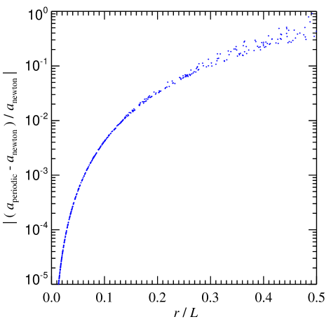
Figure 2: Force law for an isolated point mass in a cubic periodic box of size $L$ relative to the Newtonian force. The force is nowhere equal to the Newtonian force, but it becomes close to it in the immediate vicinity of a point mass. But even there, using the Newtonian force at distances above $\sim 1$ percent of the box size already produces a relative force error in excess of $10^{-5}$. This deviation due to the infinite periodic grid of image masses quickly grows at larger distances, and reaches of order unity at separations approaching half the box size. There, the effective force law also becomes decidedly non-isotropic, reflected in the scatter seen at fixed $r$.

2.1 Softened potential in periodic systems

The peculiar gravitational potential $\phi({\bf x})$ produced by $N$ particles with masses $m_{j}$ at coordinates ${\bf x}_{j}$ in a domain of dimensions $L_{x}\times L_{y}\times L_{z}$ that is periodically replicated in all three directions is given by

$$\phi({\bf x})=-\sum_{j=1}^{N}\sum_{{\bf n}=-\infty}^{\infty}\left\{\frac{m_{j}}{|{\bf x}_{j}-{\bf x}+{\bf q}_{\bf n}|+\epsilon(|{\bf x}_{j}-{\bf x}+{\bf q}_{\bf n}|)}-m_{j}\varphi_{{\bf n}}({\bf x})\right\}.$$ (1)

Here ${\bf q}_{\bf n}$ denotes periodic displacement vectors given by ${\bf q}_{\bf n}=(n_{x}L_{x},n_{y}L_{y},n_{z}L_{z})$, where ${\bf n}=(n_{x},n_{y},n_{z})$ are integer triplets and the sum over ${\bf n}$ extends over all these triplets. The gravitational constant $G$ has been omitted for simplicity. The potential contribution $\varphi_{\bf n}({\bf x})$ is that of a homogenous cuboid of unit mass and extension $L_{x}\times L_{y}\times L_{z}$ at displacement position ${\bf q}_{\bf n}$. This term is needed to allow for convergence of the infinite sum over the periodic system by effectively establishing gravitational charge neutrality. Despite adding this term, the sum over ${\bf n}$ is still only conditionally convergent, such that the answer can depend on the order of how one sums over the periodic grid. For example, summing in spherical shells up to some maximum radius produces an additional force component if the dipole moment of the fundamental box is non-zero (de Leeuw, Perram & Smith, 1980), which is however absent if one manages to truly sum the infinite grid via Ewald summation (see below). Note that in the latter case, the added homogeneous density contribution cannot generate any force due to translational symmetry.

Note that one would in principle be free to add any constant of choice to the potential given in equation (1), allowing a shift of the zero-point of the potential. Our choice corresponds to the convention that the potential is zero for vanishing density fluctuations. For isolated boundary conditions, we instead use the familiar choice of putting the zero point of the potential at infinity, making it negative everywhere. Note that for periodic boundaries, ‘infinity’ does not really exist. In either case, this does not affect any of the physics, as only the gradient of the potential enters the dynamics, and for the gravitational unbinding computations in the SUBFIND algorithm, only potential differences between two points are considered, such that the zero point of the potential drops out.

The function $\epsilon(r)$ describes a gravitational softening law. We shall assume that the softening has finite range, with $\epsilon(r)=0$ for $r\geq r_{0}$, and with $r_{0}$ being smaller than half the smallest box dimension. Specifically, we adopt the same softening law as in previous GADGET versions, in which the potential of a point particle is replaced by the potential of a smoothed mass distribution with an outer edge at $h=2.8\,\epsilon_{0}$, where $\epsilon_{0}$ is the softening length. The latter gives the depth of the potential, $-Gm/\epsilon_{0}$, at zero lag. In the above notation, this softening law can be expressed as

$$\epsilon(r;\epsilon_{0})=-\frac{2.8\epsilon_{0}}{W_{2}(r/2.8\epsilon_{0})}-r,$$ (2)

where the function $W_{2}(u)$ is given in Springel, Yoshida & White (2001, their eqn. 71). In Figure 1, we show the shape of the softening law $\epsilon(r;\epsilon_{0})$. Note that while the softening only vanishes completely for distances above $2.8\,\epsilon_{0}$, the onset of the softening happens very gradually and only starts to become significant for $r\sim 1.0\,\epsilon_{0}$, hence we identify $\epsilon_{0}$ as the length scale characterizing the gravitational softening length.

If we define ${\bf q}^{\star}_{j}({\bf x})$ (or ${\bf q}_{j}^{\star}$ for short) as the periodic displacement that minimizes the distance of ${\bf x}_{j}+{\bf q}_{\bf n}$ to ${\bf x}$ (in other words, ${\bf q}_{j}^{\star}({\bf x})$ selects the nearest periodic image location of particle $j$ to the position ${\bf x}$), we can write the potential as

$$\phi({\bf x}) = -\sum_{j=1}^{N}\frac{m_{j}}{|{\bf x}_{j}-{\bf x}+{\bf q}_{j}^{\star}|+\epsilon(|{\bf x}_{j}-{\bf x}+{\bf q}_{j}^{\star}|)}$$ (3)

$$+\sum_{j=1}^{N}m_{j}\psi({\bf x}_{j}-{\bf x}+{\bf q}_{j}^{\star}),$$

where we have introduced a correction potential given by

$$\psi({\bf x})=\frac{1}{|{\bf x}|}-\sum_{{\bf n}=-\infty}^{\infty}\left\{\frac{1}{|{\bf x}+{\bf q}_{{\bf n}}|}-\varphi_{{\bf q}_{{\bf n}}}({\bf x})\right\},$$ (4)

and made use of the fact that the softening of distant images vanishes. The potential can thus be computed as the ordinary (softened) potential from the nearest periodic image of each particle, modified by a correction term which is the difference between the negative point potential of this nearest image and an infinite periodic grid of points. Note that the selection of the nearest image for the calculation of the direct interaction ensures that it is this interaction that is affected by softening (if any), keeping the softening length out of the definition of $\psi({\bf x})$.

It is important to realize that taking just the Newtonian force of the nearest image is nowhere adequate. Figure 2 shows the difference between the full periodic force and just the Newtonian force of the nearest image. Even for distances as small as $\sim 1$ percent of the box size, the correct force differs systematically by $\simeq 10^{-5}$ from the Newtonian force, a deviation that quickly grows for larger separations. Approximating the force as Newtonian below a certain distance therefore leads to a biased force. For distances of order half the box size, the difference to the Newtonian force reaches order unity and the real periodic force shows significant deviations from spherical symmetry.

The sum in equation (4) is only conditionally convergent. Summing it in spherical shells is possible with a convergence factor, but convergence is extremely slow nevertheless. However, using Ewald’s technique (Ewald, 1921) the sum can be decomposed into two sums that individually converge very rapidly and absolutely. This decomposition can be written as

$$\psi({\bf x}) = \frac{1}{|{\bf x}|}+\frac{\pi}{\alpha^{2}V}-\sum_{{\bf n}}\frac{{\rm erfc}(\alpha|{\bf x}+{\bf q}_{\bf n}|)}{|{\bf x}+{\bf q}_{{\bf n}}|}-$$ (5)

$$\frac{4\pi}{V}\sum_{{\bf k}\neq 0}\frac{\exp[-{|{\bf k}|^{2}}/({4\alpha^{2})}]}{|{\bf k}|^{2}}\cos\left({\bf k}\cdot{\bf x}\right),$$

where $V=L_{x}L_{y}L_{z}$ is the volume of the domain. The first sum still extends over all periodic images ${\bf q}_{\bf n}$, given by ${\bf q}=(n_{x}L_{x},n_{y}L_{y},n_{z}L_{z})$ with $(n_{x},n_{y},n_{z})\in\mathbb{Z}^{3}$, but is now rapidly converging in real space thanks to the cut-off introduced by the complementary error function. The second sum extends over ${\bf k}\in\{2\pi(n_{x}/L_{x},n_{y}/L_{y},n_{z}/L_{z})\;:\;(n_{x},n_{y},n_{z})\in\mathbb{Z}^{3}\}$ in frequency space and is just the discrete periodic Fourier transform of the $4\pi/{\bf k}^{2}$ Green’s function of Poisson’s equation, decorated with an exponential short range cut-off factor $\exp[-r_{s}^{2}|{\bf k}|^{2}]$, where $r_{s}=1/(2\alpha)$ can be interpreted as a force split scale between the short-range part given by the first sum, and the long-range part given by the second sum.

Physically, Ewald summation can be understood as adding a negative, spatially extended screening mass with a Gaussian profile around every point mass. This leads to vanishing contributions of distant point masses of the infinite grid, so that the corresponding sum now converges rapidly. Of course, the added smooth negative mass has to be compensated by adding the same positive contribution. But this corresponding potential contribution can now be summed efficiently as a rapidly converging Fourier series, because the grid of Gaussian mass distributions is very smooth. Note that the correction potential has a finite value at the origin; for a cubic box of size $L$ we have $\psi({\bf x}\to 0)=2.8372975/L$.

With the Ewald formula in hand, we have a method that allows the direct summation computation of the potential for an arbitrary periodic point distribution to machine precision. Note that this provides the one and only correct solution to the problem – all other force calculation algorithms should be benchmarked against this reference. Such alternative algorithms are of course in critical demand, as direct summation is much too slow for large particle numbers.

There are many different possible approaches for approximately calculating equation (3) in practice. Particle-mesh methods create a density field on a grid and discretize Poisson’s equation directly, which is then either solved with Fourier methods, or in real space with iterative multi-grid solvers. The primary disadvantage of these methods is that the force softening law cannot be freely chosen. Rather it is directly tied to the mesh geometry, with no/poor resolution below the grid scale and anisotropic force errors at the grid scale, i.e. the error in solving for the force can be relatively large. Adaptive mesh refinement and particle-particle corrections can partially address these limitations but the effective resulting force law is usually still not particularly clean, and it will in general be extremely hard if not impossible to guarantee force errors below any prescribed level for general particle distributions, in particular highly clustered ones.

We therefore prefer so-called tree algorithms that evaluate the short-range forces via hierarchical multipole expansions. We have implemented in GADGET-4 different flavours of such schemes, these are (1) a classic Barnes & Hut (1986) style tree combined with a new type of Ewald correction when periodic boundaries are used, (2) a TreePM approach where long-range forces are computed with Fast Fourier techniques and short-range forces are evaluated with the tree, (3) a Fast Multipole Method (FMM) where the tree is accelerated by multipole expansion both at the source and sink sides, and an Ewald correction is used to implement periodic boundaries if present, and (4) a FMM-PM-approach where the PM approach is combined with FMM for the short-range forces. Both for the classic one-sided tree and the FMM, the expansion order can be varied in the present implementation up to triakontadipole order in the potential, and hexadecupole order in the force. We now discuss these methods in turn.

2.2 Tree algorithm

2.2.1 Geometry of the tree

As standard tree algorithm, we employ a classic Barnes & Hut (1986) oct-tree that is constructed through hierarchical subdivision of tree nodes. All particles are mapped onto a finely resolved space-filling Peano-Hilbert curve, which can be naturally cut into a hierarchy of nested cubes which are commensurable with the geometric structure of the oct-tree (see Springel, 2005, for a discussion of this space-filling curve). We exploit this property also in the domain decomposition to effectively distribute branches of a fiducial global tree to local MPI ranks, i.e. the fact that the tree is distributed in memory neither affects the geometry of any of the tree nodes nor the interactions lists we process.

In GADGET-2/3, we employed a fully refined tree where a new cubical node of half the parent’s size is introduced whenever more than one particle fall into the same octant of a node. This eliminates the need for an arbitrary threshold for the maximum number of particles in a node, but it has the disadvantage that two particles may never be at the same location, otherwise the tree construction would fail as these particles could not be split apart. We therefore now allow for the setting of a certain threshold particle number, and only when a tree leaf node contains more particles than this value, the tree node is split, similar to the approach adopted by other tree codes (e.g. PKDGRAV, Potter, Stadel & Teyssier, 2017). As a welcome side effect, this can reduce the total number of nodes substantially, thus reducing the memory requirements. It can also have a mild positive speed impact if the threshold is in the range of a few, because then the evaluation of some of the comparatively complicated node-particle interactions is traded in for a larger number of simpler particle-particle interactions, which can still end-up being slightly faster.

2.2.2 One-sided multipole expansion

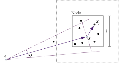
Figure 3: Sketch of a tree node and the geometry of our adopted opening angle definition and minimal distance zone around the node. The centre-of-mass position ${\bf s}$ of the particles in the cubical box of size $l$ has a distance $r$ to the force evaluation point ${\bf x}$, so that the node is seen under an angle of $\theta=l/r$. Comparison of this angle to a critical opening angle determines whether the multipole expansion of the node may be used or not. Additionally, we typically require that ${\bf x}$ lies outside an exclusion region of side length $2\,l$ centred on the cube, in order to protect against pathological force errors that could otherwise arise if ${\bf s}$ lies on the far side of the cube while ${\bf x}$ comes close to a particle on its near side.

The gravitational potential generated by the points inside a node is

$$\Phi({\bf x})=-G\sum_{j\,\in\,{\rm node}}m_{j}\,g({\bf x}_{j}-{\bf x}),$$ (6)

where $g({\bf x})=g(-{\bf x})$ is the Green’s function of the interaction, i.e. $g({\bf x})=1/|{\bf x}|$ for the Newtonian case, or the more complicated kernel of equation (3) for the periodic case. We now select the centre-of-mass ${\bf s}$ of the points in the node for a Taylor expansion of the potential around this point, yielding

$$\Phi({\bf x})=-G\sum_{n=0}^{p}\frac{1}{n!}{\bf Q}_{n}\cdot{\bf D}_{n}({\bf s}-{\bf x})\;+\;\mathcal{O}(\theta^{p+1})$$ (7)

up to order $p$ of the expansion, with $\theta$ being the characteristic angular extension under which the particle group is seen. Here we introduced the Cartesian multipole moments

$${\bf Q}_{n}\equiv\sum_{j\,\in\,{\rm node}}m_{j}({\bf x}_{j}-{\bf s})^{(n)},$$ (8)

and derivative tensors

$${\bf D}_{n}={\bf\nabla}^{(n)}g({\bf x}).$$ (9)

The notation ${\bf x}^{(n)}$ refers to the $n$-th outer product of the vector (or tensor) with itself, while ${\bf x}\cdot{\bf y}$ denotes the inner product (i.e. contraction) of two vectors or tensors. Currently, GADGET-4 supports a selection of $p=1$, 2, 3, 4, or 5 at compile time, i.e. the multipole expansion of the potential field of a node is carried out to dipole, quadrupole, octupole, hexadecupole, or triakontadipole order, respectively. Since we expand around the center-of-mass of each node, the dipole moment always vanishes, and $p=1$ means in practice that only monopole terms need to be considered, i.e. $p=1$ is equivalent to $p=0$ for the potential.

Similarly, the acceleration exerted on a test mass at location ${\bf x}$ can be written as

$${\bf a}({\bf x})=-\nabla\Phi({\bf x})=-G\sum_{n=0}^{p-1}\frac{1}{n!}{\bf Q}_{n}\cdot{\bf D}_{n+1}({\bf s}-{\bf x})\;+\;\mathcal{O}(\theta^{p})$$ (10)

to order $p-1$ of the expansion. Compared to a direct differentiation of equation (7), we here dropped the last term in the expansion in order to end up with the same highest order in the derivative tensor for a specified $p$, both for potential and force, and to make the one-sided tree behave more similar to the FMM algorithm (where the accuracy of the force is one order lower than that of the potential, see later on). Note that a side effect of this is that the force accuracies obtained for $p=1$ and $p=2$ are equal in the one-sided tree. As we shall see later on, which order $p$ is most efficient can be problem dependent. Using higher order is in general more efficient if one aims very low force errors, but it also entails a higher peak memory usage because more multipole moments need to be stored for the nodes.

Note that the multipole tensors ${\bf Q}_{n}$ are totally symmetric (i.e. elements where two indices are interchanged are equal), so that they feature only $(n+2)(n+1)/2$ independent elements at order $n$. If the interaction kernel is isotropic like in the ordinary Newtonian case, or if the periodic boundary conditions impose cubical symmetry, the derivative tensors are totally symmetric as well. This reduces the storage requirements substantially and also simplifies many of the algorithmic operations with them, which we try to exploit as much as possible. If the interaction potential is a simple power-law in radius, like for Newtonian gravity, it turns out be sufficient to store the multipole moments in a trace-free form, where the number of independent elements is reduced further to $2n+1$, which can save a substantial amount of memory for high expansion orders (Coles & Bieri, 2020). In this case, the Cartesian formulation is closely analogous to an expansion into spherical harmonics, as used in the original formulation of FMM (Greengard & Rokhlin, 1987). However, since this optimisation is not viable for periodic boundary conditions, which is the most important case for cosmology, we refrain from considering it here. It would however still be of interest as a possible future extension for isolated boundary conditions.

2.2.3 Tree walk and opening criterion

In the force calculation for a given particle, the tree is walked top-down, starting at the root node. For deciding whether or not a multipole expansion of the current node is acceptable, different criteria can be used. We either adopt a straightforward classical geometric opening criterion, as sketched in Figure 3, according to which the multipole expansion of a node can be used if

$$\frac{l}{r}<\theta_{c},$$ (11)

where $l$ is the side-length of the cubical tree node, $r$ is the distance of the target coordinate to the node’s centre of mass, and $\theta_{c}$ is a critical angle controlling the accuracy (as well as computational cost) of the force approximation. Alternatively, a relative opening criterion as first proposed by Springel, Yoshida & White (2001) can be used, where a rough approximation of the expected force error is compared with the magnitude of the total force,

$$\frac{M}{r^{2}}\left(\frac{l}{r}\right)^{p}<\alpha|{\bf a}|,$$ (12)

where $|{\bf a}|$ is the total acceleration, usually estimated for a particle from the force obtained in the previous timestep. The parameter $\alpha$ controls the force accuracy.

This second criterion aims at achieving a more or less constant force error in every individual interaction, and the size of this error is chosen in relation to the magnitude of the final force. This means that nodes that are more important for the final force are evaluated with higher relative force accuracy than less important contributions, which gives a more economical scheme overall. Also, the final relative force accuracy is roughly kept constant for all particles, independent of clustering state. This is especially useful for cosmological simulations where the peculiar forces at high redshift are small due to near cancellation of forces in all different directions. In this situation, the relative opening criterion automatically invests more effort, whereas in strongly clustered regions most of the effort is concentrated in evaluating the dominant force components. This automatic adjustment to the clustering state is a welcome feature in these types of calculations. Indeed, in Springel (2005) it was shown that the relative criterion is typically more efficient than the geometric one in the sense of delivering higher force accuracy than the geometric criterion at a given computational cost, something that we will verify here later on as well.

We typically augment both of the above criteria with an additional geometric test that prevents the use of multipole expansions if the distance to the geometric center of a tree node is less than $l$. This corresponds to an exclusion zone around the tree node’s geometric centre, as sketched in Figure 3. This is a simple conservative means to protect against pathological cases that could occur if one allows evaluations of multipoles for reference points very close to or even within nodes (see also Salmon & Warren, 1994). It also prevents a complete break-down of the convergence of the Taylor expansion if the opening criterion would otherwise allow an extremely large opening angle.

2.2.4 Periodic boundary conditions

If periodic boundaries are desired for the pure tree method, additional complications arise as we have to cope with the infinite sum of equation (1). The approach followed in previous versions of GADGET consists of exploiting equation (3) directly for each node or particle interaction. This means that during the tree walk every node (or single particle when encountered) is mapped to its nearest periodic image relative to the coordinate of the force evaluation. If the node does not have to be opened, the first term in equation (3) can be evaluated by means of a multipole expansion with the normal Newtonian Green’s function. The second term can also be evaluated with a multipole expansion, but now relies on the Green’s function $\psi({\bf x})$ defined in equation (5), which does not have a closed form expression. One can compute it with the rapidly converging Ewald sum, but as this needs to be evaluated for every interaction, a substantial computational cost is incurred.

Another solution is to tabulate the correction potential (which is quite smooth) and its derivatives in a three-dimensional pre-computed look-up table, from which one then calculates $\psi$ and its derivatives as needed by tri-linear interpolation. This is what we had previously done in GADGET, following a similar approach as in Hernquist, Bouchet & Suto (1991) Our default look-up table size has used $64^{3}$ entries (for one octant only, the rest can be inferred due to the symmetries involved), and we used separate tables for the potential and the three spatial components of the force, which is sufficient for $p=1$. Perhaps the worst disadvantage of this approach is that its accuracy is fundamentally limited by the interpolation accuracy of the look-up table, making it hard to push the relative force errors below $\sim 10^{-3}$. If this is nevertheless desired, one either has to make the lookup table sufficiently fine, which soon becomes prohibitive due the unacceptably large amounts of memory consumed by a three-dimensional table with many entries per dimension, or come up with a different approach that allows a more accurate but still fast way to compute the interaction tensors.

To obtain the desired high accuracy for ${\bf D}_{n}$, we have replaced the trilinear interpolation from a look-up table with a scheme based on Taylor expansions. We still precompute a grid for the ${\bf D}_{n}$, but to obtain the value at a given coordinate ${\bf x}$, we first locate the closest point ${\bf x}_{0}$ to ${\bf x}$ in our grid, and then approximate the target value through the expansion

$${\bf D}_{n}({\bf x}) \simeq {\bf D}_{n}({\bf x}_{0})+{\bf D}_{n+1}({\bf x}_{0})\cdot\Delta{\bf x}+\frac{1}{2}{\bf D}_{n+2}({\bf x}_{0})\cdot\Delta{\bf x}^{(2)}$$ (13)

$$+\;\frac{1}{6}{\bf D}_{n+3}({\bf x}_{0})\cdot\Delta{\bf x}^{(3)},$$

of the interaction kernel, where $\Delta{\bf x}={\bf x}-{\bf x}_{0}$. Since we want ${\bf D}_{n}$ up to order $n=5$, we actually tabulate the tensors up to order $n=8$ on the grid. The pre-computation of these tensors is done based on analytic derivatives of the Ewald summation formula, and hence can be easily made exact up to machine precision. The Taylor expansion approach is much more accurate than tri-linear interpolation. It gives us the ability to recover all needed derivative tensors to a relative accuracy of $\simeq 10^{-10}$ for arbitrary interaction distance ${\bf x}$; only if this is achieved, the high-order versions of the multipole methods ultimately make sense and converge properly to the direct summation result also for difficult situations such as cosmological initial conditions at high redshift.

2.3 TreePM approach

An alternative to the pure tree algorithm that avoids the need for explicit Ewald corrections is the so-called TreePM approach (Xu, 1995; Bagla, 2002; Springel, 2005). In this method, we adopt in equation (5) a value of $r_{s}=1/(2\alpha)$ that is very small against the box size, i.e. $r_{s}\ll\min(L_{x},L_{y},L_{z})$. In this case, we can restrict the real-space sum over the nearest periodic images exclusively to the ${\bf q}=0$ term, resulting in a total short-range potential of the form

$$\phi_{\rm sr}({\bf x})=\sum_{j}m_{j}\left\{\frac{-1}{|{\bf r}_{j}|+\epsilon(|{\bf r}_{j}|)}+\frac{1}{|{\bf r}_{j}|}+\frac{\pi}{\alpha^{2}V}-\frac{{\rm erfc}(\alpha|{\bf r}_{j}|)}{|{\bf r}_{j}|}\right\},$$ (14)

where ${\bf r}_{j}=|{\bf x}-{\bf x}_{j}+{\bf q}^{\star}|$ denotes the nearest periodic distance of $j$ to the reference point. This can be evaluated with a tree algorithm in real space, while the frequency sum gives a long range potential of the form,

$$\phi_{\rm lr}({\bf x})=\sum_{j=1}^{N}m_{j}\,\frac{4\pi}{V}\sum_{{\bf k}\neq 0}\frac{\exp[-{|{\bf k}|^{2}}/({4\alpha^{2})}]}{|{\bf k}|^{2}}\cos\left[{\bf k}\cdot({\bf x}-{\bf x}_{j})\right],$$ (15)

which can be computed through Fourier methods, as described below. TreePM is thus best understood as a special version of the Ewald summation technique, where the total potential of eqn. (3) is obtained as $\phi({\bf x})=\phi_{\rm sr}({\bf x})+\phi_{\rm lr}({\bf x})$. We note that it would in principle be possible to employ a different cut-off function to separate short-range and long-range forces. Using the complementary error function in real space is associated with a rapidly and monotonically declining exponential filter in $k$-space, which is essentially as good as it gets. Still more sharply declining real-space cut-off functions will in general require more complicated $k$-space filters that may need empirical calibration but could then also be viable.

For calculating the force corresponding to $\phi_{\rm sr}$ with a tree walk we proceed as in the ordinary tree algorithm, except that we use different expressions for evaluating the multipole contributions that reflect the modification of the inverse distance potential due to the short-range cut-off. We keep in principle the same opening criteria as used in the ordinary tree walk, except that we add the further criterion that a tree node is dropped entirely from consideration if its nearest edge is further away than a distance $r_{\rm cut}$, where the force has become unsoftened and the cut-off factor ${\rm erfc}(\alpha\,r)$ is so large that the ordinary Newtonian potential is heavily suppressed. We set $r_{\rm cut}=\max[R_{\rm cut}\times r_{s},2.8\epsilon_{0}]$, where the precise value adopted for the dimensionless parameter $R_{\rm cut}\simeq 4.5-7.0$ affects both the computational cost and the residual force errors in the matching region between the short-range and long-range forces. If a maximum relative force error of order $10^{-2}$ is sufficient, one can choose $R_{\rm cut}$ as small as $\simeq 4.5$ for maximum computational speed, but if lower maximum force errors are desired, larger cut-off values need to be chosen. For $R_{\rm cut}=7$, the suppression factor for the potential and the force relative to the Newtonian value reach around $10^{-5}$ at the cut-off radius. The cut-off radius effectively restricts the tree walk to a small spherical region around the evaluation point, yielding a significant gain in performance compared to a full tree walk. In addition, no Ewald corrections need to be computed for the short-range force. These two factors can make TreePM faster than the ordinary tree algorithm, provided the speed-up is not offset by the cost of the additionally required PM calculation.

For efficiently evaluating the short range force kernel of equation (14) and its derivatives, we use linear interpolation from a small one-dimensional look-up table. This avoids the costly computation of the complementary error function for every interaction. Again, depending on the desired accuracy goals, the length of this table can be varied. A finer look-up table yields smaller residual interpolation errors but reduces the cache efficiency of the processor. If maximum relative force errors as low as $10^{-5}$ are desired, we use a table with 256 entries, for more commonly employed force accuracies such as $10^{-3}$, already 48 entries are in principle sufficient.

We note that if the softening length is much smaller than the split scale $r_{s}$, which is almost always the case, equation (14) can be approximated as

$$\phi_{\rm sr}({\bf x})\simeq-\sum_{j}m_{j}\frac{{\rm erfc}(\alpha|{\bf r}_{j}|)}{|{\bf r}_{j}|+\epsilon(|{\bf r}_{j}|)},$$ (16)

which had been adopted in GADGET-2 (omitting also the constant $\pi m_{j}/(\alpha^{2}V)$ term in the potential for simplicity, which does not contribute to the dynamics). However, since one may not necessarily always have $\epsilon_{0}\ll r_{s}$, GADGET-4 uses the more accurate expression (14).

The Fourier sum of equation (15) can be recognized as the inverse Fourier transform of the product of the Green’s function $\exp(-r_{s}^{2}{\bf k}^{2})/{\bf k}^{2}$ with the Fourier transform of a density field in which each particle is represented by a Dirac $\delta$-function. This can be solved with a standard particle-mesh approach (e.g. Hockney & Eastwood, 1988) in which we first create a binned density field, for example through clouds-in-cell (CIC) assignment, calculate a discrete Fast Fourier Transform (FFT), multiply with the Green’s function, and then transform back to obtain the potential. The forces can then be obtained on the same grid through finite differencing, followed by interpolating them to the particle positions. The smoothing effects of the assignment and interpolation operators can be compensated in the mean by deconvolving with their corresponding Fourier transforms, which in the case of CIC corresponds to a division with a sinc-function. We use a 4-th order accurate finite differencing formula on the potential grid to derive the forces. Using spectral differencing instead would be possible as well, but this is computationally more costly due to the larger number of Fourier transforms required (and larger memory needs for retaining an auxiliary copy of the field) while it does not provide significant accuracy advantages.

The resulting long-range forces are accurate provided the Nyquist frequency of the employed mesh is large enough to include all frequencies significantly contributing to the long-range potential. Fortunately, the exponential cut-off factor in the Green’s function introduces a well-defined scale beyond which the Fourier spectrum of the potential declines rapidly in a smooth and isotropic fashion, an important advantage over ordinary PM and P³M schemes. For high accuracy we need $\exp(-k^{2}_{\rm Nq}r_{s}^{2})\ll 1$, where $k_{\rm Nq}=(2\pi/L)(N_{\rm grid}/2)$ and $N_{\rm grid}$ is the number of grid points per dimension. In practice, we define the dimensionless parameter $A_{\rm smth}=r_{s}/(L/N_{\rm grid})$ and use it to parameterize the transition scale for a given mesh size $N_{\rm grid}$, yielding $\exp(-k^{2}_{\rm Nq}r_{s}^{2})=\exp(-\pi^{2}A_{\rm smth}^{2})$. The value of this factor drops to about $2\times 10^{-7}$ for our “fastest runtime” but least conservative setting of $A_{\rm smth}=1.25$. Larger values of $A_{\rm smth}$ for a given mesh size $N_{\rm grid}$ imply that more Fourier modes are invested to sample the high-frequency decline of the long-range force. This makes the long-range force more accurate, but also implies that the cut-off $r_{\rm cut}$ moves to larger scales, so that the short-range tree force has to be evaluated over a larger region, increasing its relative computational cost. By varying $A_{\rm smth}$ one can thus smoothly change the force accuracy of the long-range force, and shift the balance in the computational cost between PM and tree. Depending on the desired final force accuracy, different sweet spots for maximum computational efficiency exist. We will return to this point in Section 3 when we systematically investigate the force accuracy and relative computational cost of the different gravity solvers available in GADGET-4.

For the evaluation of the Fourier transforms in the TreePM approach we employ the Fast Fourier Transform algorithm as implemented in the FFTW library (Frigo & Johnson, 2005). We employ the current version 3 of FFTW but refrain from using its built-in MPI-parallelized functions, instead we employ our own parallelization layer on top of one-dimensional real-to-complex and complex-to-complex FFTs provided by the library. This was done to avoid that dynamic memory allocation is used outside of GADGET-4’s direct control, which can create problems if one operates very close to the physical memory limit and does large FFTs nevertheless. It also allows us to seamlessly switch to a column-based data decomposition when required for scalability, which is presently not supported by the MPI interface of FFTW-3. More details on this, in particular the column-based data decomposition, are given in Section 6.4 on parallelization.

2.4 Fast multipole method

The so-called fast multipole method (FMM) has been originally introduced by Greengard & Rokhlin (1987) and is arguably the fastest known approach for hierarchical multipole expansion when high force accuracy is required, improving upon the ‘one-sided’ tree algorithm of Barnes & Hut (1986). A variant of the original harmonic FMM approach that treats all expansions in Cartesian coordinates instead of using spherical harmonics has first been introduced by Dehnen (2000, 2002). The FMM approach can be faster than a classic tree because the multipole expansion is not only carried out at the source side but also on the sink side where the target particles are located. This allows one to calculate the expansion between two well-separated “source” and “sink” nodes only once, and effectively reuse it for all particles making up the nodes, whereas in the one-sided tree it is computed many times over, more or less for each of the constituent particles on the sink side yet again with only slightly shifted expansion centres. Barnes’ (1990) grouping algorithm for the one-sided tree, in which a common interaction list for small particle groups is computed, represents another approach to mitigate this behaviour of the tree algorithm.

Furthermore, a symmetric Cartesian expansion delivers, at the same time, the force field of the sink node onto the source node and vice versa, yielding a manifestly momentum conserving formulation where the vector sum of all force errors adds up to zero. This is not the case for an ordinary tree algorithm, where in fact surprisingly large errors in the total momentum of a system can occur.

The speed advantage expected from FMM relative to the tree code has not been confirmed in all practical implementations (e.g. Capuzzo-Dolcetta & Miocchi, 1998), but this may well originate in the complexity of the spherical harmonics expansion approach used in the originally proposed method. However, Dehnen (2000) has shown that in the low-accuracy regime relevant for collisionless dynamics the Cartesian expansion variant of FMM represents an attractive formulation that can offer a significant performance advantage compared with ordinary tree methods. Still, the FMM method has thus far not been applied nearly as widely in astrophysics as classical tree algorithms, even though this has begun to change recently. The reasons presumably lie in FFM’s somewhat higher algorithmic complexity, difficulties in using it efficiently with local timestepping, in harder parallelization, and in intricacies related to the inclusion of periodic boundaries. For the present work, we have outfitted GADGET-4 with an FMM module as an alternative to the one-sided classic tree, allowing us to explore to what extent these issues can be overcome in our code in practice.

Our basic FMM approach closely follows the algorithm first presented by Dehnen (2000), but is augmented with parallelization on distributed memory machines, with treatments of multiple gravitational softening lengths and periodic boundary conditions, and with the possibility to couple FMM with a long-range PM approach, creating a FMM-PM method in analogy to the TreePM approach discussed above.

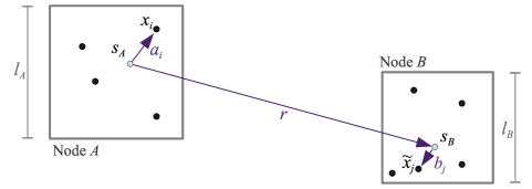
Figure 4: Sketch of the geometry and nomenclature we use to describe an FMM interaction between two nodes $A$ and $B$ of sizes $l_{A}$ and $l_{B}$. The particles in the nodes have positions ${\bf x}_{i}$ and ${\bf\tilde{x}}_{j}$, giving rise to centre-of-mass positions ${\bf s}_{A}$ and ${\bf s}_{B}$ of the nodes, respectively, with ${\bf r}={\bf s}_{B}-{\bf s}_{A}$ being their distance vector, and ${\bf a}_{i}$ and ${\bf b}_{j}$ denoting the relative positions of the particles in the nodes to their corresponding center of mass locations.

The method starts by considering the interaction potential between the particles of two nodes $A$ and $B$, as sketched in Figure 4, with ${\bf x}_{i}$ denoting the positions of the particles in $A$, and ${\bf\tilde{x}}_{i}$ those in $B$. We can write the gravitational potential generated by the points of $B$ at a particle coordinate in node $A$ as

$$\Phi({\bf x}_{i})=-G\sum_{j}m_{j}\,g({\bf\tilde{x}}_{j}-{\bf x}_{i}),$$ (17)

where $g({\bf x})=g(-{\bf x})$ is the symmetric Green’s function of the interaction. In the non-periodic case without gravitational softening, we have the simple Newtonian $g({\bf x})=1/|{\bf x}|$ interaction. With periodic boundary conditions, $g({\bf x})$ also depends on the direction of ${\bf x}$.

We now Taylor-expand the potential by introducing expansion centres both in $A$ and $B$. Obvious choices for them are either the geometric centres of the nodes, or their centres of mass; we adopt the latter as this leads to vanishing dipole moments. Let ${\bf s}_{A}$ and ${\bf s}_{B}$ denote the centres of mass in the nodes, and ${\bf r}={\bf s}_{B}-{\bf s}_{A}$ be their relative distance vector. Further, let ${\bf a}_{i}={\bf x}_{i}-{\bf s}_{A}$ be the relative position of the points in $A$ with respect to node $A$’s center of mass, and likewise ${\bf b}_{i}={\bf\tilde{x}}_{i}-{\bf s}_{B}$ for node $B$. We then have ${\bf\tilde{x}}_{j}-{\bf x}_{i}={\bf r}+{\bf b}_{j}-{\bf a}_{i}$, and obtain up to $p$-th order for the interaction potential

$$g({\bf\tilde{x}}_{j}-{\bf x}_{i})\simeq\sum_{n=0}^{p}\frac{1}{n!}{\bf\nabla}_{{\bf r}}^{(n)}g({\bf r})\cdot({\bf b}_{j}-{\bf a}_{i})^{(n)},$$ (18)

assuming $|{\bf a}_{i}|\ll|{\bf r}|$ and $|{\bf b}_{j}|\ll|{\bf r}|$ (well separatedness of the nodes). Again, here the notation ${\bf x}^{(n)}$ means the $n$-th outer product of the vector with itself, while ${\bf x}\cdot{\bf y}$ denotes the inner product (i.e. contraction) of two vectors or tensors. Expanding the term involving the relative positions into a binomial series,

$$({\bf b}_{j}-{\bf a}_{i})^{(n)}=\sum_{k=0}^{n}\left(\begin{array}[]{c}n\\ k\\ \end{array}\right){\bf b}_{j}^{(n-k)}(-{\bf a}_{i})^{(k)},$$ (19)

and rearranging the sums yields

$$g({\bf\tilde{x}}_{j}-{\bf x}_{i})\simeq\sum_{k=0}^{p}\frac{(-1)^{k}}{k!}{\bf a}_{i}^{(k)}\cdot\sum_{n=0}^{p-k}\frac{1}{n!}{\bf\nabla}^{(n+k)}g({\bf r})\cdot{\bf b}_{j}^{(n)}.$$ (20)

By introducing the multipole moments

$${\bf Q}^{B}_{n}\equiv\sum_{j}m_{j}{\bf b}_{j}^{(n)},$$ (21)

we hence arrive at

$$\Phi({\bf x}_{i})\simeq-G\sum_{k=0}^{p}\frac{(-1)^{k}}{k!}{\bf a}_{i}^{(k)}\cdot\sum_{n=0}^{p-k}\frac{1}{n!}{\bf D}_{n+k}\cdot{\bf Q}^{B}_{n}$$ (22)

for the potential, where we have defined the $m$-th order tensors

$${\bf D}_{m}={\bf\nabla}^{(m)}g({\bf r}),$$ (23)

just like for the tree algorithm. Similarly, the potential $\tilde{\Phi}({\bf\tilde{x}}_{i})$ at a location of a point in $B$ due to the particles in $A$ is given to the same order of the expansion as

$$\tilde{\Phi}({\bf\tilde{x}}_{i}) \simeq -G\sum_{k=0}^{p}\frac{(-1)^{k}}{k!}{\bf Q}_{k}^{A}\cdot\sum_{n=0}^{p-k}\frac{1}{n!}{\bf D}_{n+k}\cdot{\bf b}^{(n)}_{j}$$

$$= -G\sum_{k=0}^{p}\frac{(-1)^{k}}{k!}{\bf b}_{i}^{(k)}\cdot\sum_{n=0}^{p-k}\frac{(-1)^{n+k}}{n!}{\bf D}_{n+k}\cdot{\bf Q}^{A}_{n},$$

and hence manifest momentum conservation,

$$\sum_{i\in A}m_{i}\nabla\Phi({\bf x}_{i})+\sum_{i\in B}m_{i}\nabla\tilde{\Phi}({\bf\tilde{x}}_{i})=0,$$ (25)

is retained if these expressions are used to approximate the force from $A$ on $B$, and vice versa. Also note that the highest order multipole moments ${\bf Q}_{p}^{A/B}$ of the expansion for a given order $p$ contribute only as constants to the potential and hence do not affect the force. As only the latter is required for the particle dynamics, we typically follow Dehnen (2000) and omit the calculations of these multipoles in practice, simply dropping them in the potential, unless we explicitly retain them through a code compile-time option.

In GADGET-4, we either consider order $p=1$, $p=2$, $p=3$, $p=4$, or $p=5$. For example, for the $p=2$ case, the explicit expression for the potential expansion becomes

$$\Phi_{p=2}({\bf x})\simeq-G\left[{Q}_{0}{D}_{0}+\frac{1}{2}{\bf Q}_{2}\cdot{\bf D}_{2}-{Q}_{0}{\bf D}_{1}\cdot{\bf a}+\frac{1}{2}{Q}_{0}{\bf D}_{2}\cdot{\bf a}^{(2)}\right],$$ (26)

but as mentioned above, the spatially constant term proportional to ${\bf Q}_{2}$ may be dropped because it does not contribute to the dynamics, and hence one can avoid calculating the second moment tensor at this order if one primarily cares about the forces only. For an expansion up to quadrupole order, $p=4$, we instead have

$$\Phi_{p=4}({\bf x}) \simeq -G\left[{Q}_{0}{D}_{0}+\frac{1}{2}{\bf Q}_{2}\cdot{\bf D}_{2}+\frac{1}{6}{\bf Q}_{3}\cdot{\bf D}_{3}+\frac{1}{24}{\bf Q}_{4}\cdot{\bf D}_{4}\right.$$ (27)

$$-({Q}_{0}{\bf D}_{1}+\frac{1}{2}{\bf Q}_{2}\cdot{\bf D}_{3}+\frac{1}{6}{\bf Q}_{3}\cdot{\bf D}_{4})\cdot{\bf a}$$

$$+\frac{1}{2}\left({Q}_{0}\,{\bf D}_{2}+\frac{1}{2}{\bf Q}_{2}\,{\bf D}_{4}\right)\cdot{\bf a}^{(2)}$$

$$\left.-\frac{1}{6}{Q}_{0}{\bf D}_{3}\cdot{\bf a}^{(3)}+\frac{1}{24}{Q}_{0}{\bf D}_{4}\cdot{\bf a}^{(4)}\right].$$

Again, we typically drop in practice the term involving the hexadecupole moment ${\bf Q}_{4}$. The expansions for other orders are given in Appendix A, for definiteness.

For non-periodic boundary conditions, or for the spatial part of Ewald sums, the short-range interaction depends only on the norm $r$ of the distance vector, $g({\bf r})=g(r)$. Defining

$$g_{n}(r)\equiv\left(\frac{1}{r}\frac{{\rm d}}{{\rm d}r}\right)^{n}g(r),$$ (28)

the derivative tensors ${\bf D}_{m}$ can be expressed in this case as

$${D}_{0} = g_{0}$$ (29)

$$({\bf D}_{1})_{i} = g_{1}\,r_{i}$$ (30)

$$({\bf D}_{2})_{ij} = g_{1}\,\delta_{ij}+g_{2}{r_{i}r_{j}}$$ (31)

$$({\bf D}_{3})_{ijk} = g_{2}\,\left({\delta_{ij}r_{k}+\delta_{jk}r_{i}+\delta_{ik}r_{j}}\right)+$$ (32)

$$g_{3}\,{r_{i}r_{j}r_{k}}$$

$$({\bf D}_{4})_{ijkl} = g_{2}\left({\delta_{ij}\delta_{kl}+\delta_{jk}\delta_{il}+\delta_{ik}\delta_{jl}}\right)+$$ (33)

$$g_{3}\,\left(\delta_{ij}r_{k}r_{l}+\delta_{jk}r_{i}r_{l}+\delta_{ik}r_{j}r_{l}\,+\right.$$

$$\left.\;\;\;\;\;\delta_{il}r_{j}r_{k}+\delta_{jl}r_{i}r_{k}+\delta_{kl}r_{i}r_{j}\right)+$$

$$g_{4}\,{r_{i}r_{j}r_{k}r_{l}},$$

$$({\bf D}_{5})_{ijklm} = g_{3}\left[r_{m}\left(\delta_{ij}\delta_{kl}+\delta_{jk}\delta_{il}+\delta_{ik}\delta_{jl}\right)+\right.$$ (34)

$$\;\;\;\;\,r_{l}\left(\delta_{ij}\delta_{km}+\delta_{jk}\delta_{im}+\delta_{ik}\delta_{jm}\right)+$$

$$\;\;\;\;\,r_{k}\left(\delta_{ij}\delta_{lm}+\delta_{jm}\delta_{il}+\delta_{im}\delta_{jl}\right)+$$

$$\;\;\;\;\,r_{j}\left(\delta_{im}\delta_{kl}+\delta_{km}\delta_{il}+\delta_{ik}\delta_{lm}\right)+$$

$$\left.\;\;\;\;\,r_{i}\left(\delta_{jm}\delta_{kl}+\delta_{jk}\delta_{lm}+\delta_{km}\delta_{jl}\right)\right]+$$

$$g_{4}\,\left(\delta_{ij}r_{k}r_{l}r_{m}+\delta_{jk}r_{i}r_{l}r_{m}+\delta_{ik}r_{j}r_{l}r_{m}\,+\right.$$

$$\;\;\;\;\;\delta_{il}r_{j}r_{k}r_{m}+\delta_{jl}r_{i}r_{k}r_{m}+\delta_{kl}r_{i}r_{j}r_{m}+$$

$$\;\;\;\;\;\delta_{im}r_{j}r_{k}r_{l}+\delta_{jm}r_{i}r_{k}r_{l}+\delta_{km}r_{i}r_{j}r_{l}+$$

$$\left.\;\;\;\;\;\delta_{lm}r_{i}r_{j}r_{k}\right)+$$

$$g_{5}\,{r_{i}r_{j}r_{k}r_{l}r_{m}},$$

where $r_{i}$ denotes the $i$-th component of the vector ${\bf r}$. We spell out ${\bf D}_{6}$ and ${\bf D}_{7}$, and give explicit forms for the derivatives $g_{n}$ of $g(r)$ in Appendix A. While all these tensors are fully symmetric in their indices, they nevertheless rapidly grow in size and complexity. For orders two to five, they have 6, 10, 15, and 21 independent components, respectively.

As stressed earlier, when periodic boundary conditions are desired without the PM approach, Ewald summation is needed to realize accurate periodic boundary conditions. The full relevant interaction potential $g({\bf r})$ is not an isotropic function in this case. We here proceed similarly to the one-sided tree algorithm by splitting the interaction into a part between the nearest periodic images of two nodes, and an Ewald-correction of this interaction. The former can be calculated with the spherically symmetric Newtonian interaction potential, whereas for the latter we again employ a Taylor-series based look up from precomputed tables, absorbing the lack of rotational symmetry into this correction.

Once the grouping of particles into a hierarchy of nodes is completed in the tree construction, we precompute the multipole moments of the tree nodes recursively from the multipole moments of their daughter nodes, which constitutes the first phase of the FMM method (up to this point there is no difference to the ordinary tree code). In the second phase, we use a dual tree walk similar to Dehnen (2000) to evaluate multipole expansions both at the source and sink side for interacting pairs of nodes or particles. This is done in a symmetric fashion where each interaction is accounted for in a manifestly momentum-conserving way.

To this end, we define a function that accounts for the interaction between two cells $A$ and $B$, meaning that all particles in $A$ must receive the force from all particles in $B$ and vice versa. Further, we invoke a criterion of well-separateness (the generalization of the opening criterion) that, if fulfilled, says that the relevant interactions can be accounted for by a simultaneous multipole expansion of the mutual interaction field both at $A$ and $B$. In this case, the corresponding field expansions are stored in $A$ and $B$ (actually, they are added to whatever field expansion the nodes may already have). Otherwise, one of the two nodes (or both, which is what we will end up doing) is split into all its daughter nodes and paired up with the unsplit node, followed by calling the function again for all the newly formed pairs. Self interactions between two identical nodes (or particles) are always ignored; instead, the self-interaction is treated by calling the interaction function for all possible pairs of daughter cells in the node.

For the node opening decisions, we employ slightly modified variants of the criteria we use for the one-sided tree algorithm. If the geometric criterion is in use, a node-node interaction is evaluated if

$$\frac{l_{1}+l_{2}}{r}<\theta_{c},$$ (35)

where $l_{1}$ and $l_{2}$ are the side-lengths of the two nodes involved. For equal node sizes and the same value of $\theta_{c}$, this means that the nodes see each other typically under a smaller effective angle than in the one-sided tree algorithm, but as we see later, this is also necessary for achieving roughly comparable accuracy due to the error of the field expansion on the sink’s side that is additionally present in FMM. Similarly, we require

$$\frac{M_{\rm max}}{r^{2}}\left(\frac{l_{\rm max}}{r}\right)^{p-1}<\alpha|{\bf a}|_{\rm min},$$ (36)

for a node-node interaction when the relative opening criterion is selected in FMM. Here, $M_{\rm max}=\max(M_{1},M_{2})$ is the maximum of the two nodes’ masses and $l_{\rm max}=\max(l_{1},l_{2})$ the maximum of their side lengths. Such a simple power-law characterization of the force errors gives a typically close but not strict characterization of the errors, see Dehnen (2014), who also shows how the error estimates can be sharpened in principle by exploiting the lower order multipole moments. We define $|{\bf a}|_{\rm min}=\min(|{\bf a}|_{1},|{\bf a}|_{2})$ as the minimum acceleration occurring among any of the particles in the two nodes. The corresponding minimum $|{\bf a}|$ for every tree node is determined during tree construction as an additional node property. Note that the power with which the effective opening angle $\theta\approx l_{\rm max}/r$ enters is reduced by one unit for a given expansion order $p$ compared to the criterion used in the one-sided tree. Again, this accounts for the additional error induced by the sink-side expansion in FMM. If enabled, the use of a spatial exclusion zone around a node is the same as in the tree. In practice this means that we do not allow for interactions of nodes that directly touch.

The calculation of all interactions can simply be initiated by calling the interaction routine with two copies of the root node, with the processing of required daughter node interactions done recursively. When distributed memory parallelization is used, we nevertheless need to also employ a stack on which pairs of nodes that still need processing are temporarily stored in order to hide communication times.

Finally, in the third phase of the FMM algorithm, the field expansions are passed down the tree, translated to new expansion centres if needed, and summed in nodes, until they are eventually evaluated at particle coordinates, delivering the total potential and force for all particles. To this end, we recursively walk the tree in a top-down fashion, accumulating field expansions for the nodes by shifting the expansion centre of a node’s parent node to that of the current node (this operation is straightforward for an expansion in Cartesian coordinates), and then adding the expansion coefficients, until one arrives at single particles for which the field is evaluated and added to the force/potential the particle may already have acquired through individual cell-particle interactions in phase two above.

As noted earlier, one advantage of FMM lies in the manifest momentum conservation possible for this method, meaning that all the force errors add up to zero to machine precision. This is in general not the case for the ordinary tree algorithm. There are however also some disadvantages of FMM. One is that partial force calculations, where the number of sinks is much smaller than the number of source particles and which occur in many standard local timestep integration schemes, are not well matched to the FMM approach, because the latter is designed to compute the forces for all particles in a globally efficient way. If forces only for, say, 5% of the particles are desired, the method will not just take 5% of the computational effort, but rather something still close to the full effort. In contrast, the one-sided tree algorithm delivers “linear elasticity” in the computational cost. But we note that this disadvantage of FMM completely disappears when a hierarchical time-integration scheme (see Section 4.2) is used, because here all force calculations always involve equal sets of source and sink particles.

Another slight technical complication lies in the treatment of different gravitational softening lengths for the particles making up nodes. Finally, the parallelization of FMM for distributed memory machines is more involved than for an ordinary tree code, even though recently some successful implementations have been described (e.g. Potter, Stadel & Teyssier, 2017). Our approach for dealing with distributed memory parallelisation of FMM will be described in Section 6.

2.5 The FMM-PM approach

We can readily generalize the TreePM approach to a FMM-PM approach. The PM part is the same in both cases, only the evaluation of the short range force is now carried out with the FMM method instead of the one-sided tree. This requires a change of the real-space Green’s function $g({\bf r})$ with respect to the Newtonian case $g(r)=1/r$, just as in TreePM. Again, we use a cut-off distance $r_{\rm cut}$ and restrict the evaluation of FMM interactions to distances $r<r_{\rm cut}$. Over this range, we tabulate the interaction potential and all its higher derivatives – which are needed now for FMM – in a one-dimensional look-up table from which we interpolate with bi-linear interpolation, very similar to the TreePM approach.

Interactions between two nodes are dropped (and hence also not further refined) when the distance of their nearest sides exceeds the cut-off distance $r_{\rm cut}$. We do not modify the opening criteria themselves, however, and when the relative opening criterion is used, the estimated force errors are always compared against the total gravitational accelerations of the particles, including the PM contributions. As we will show later on explicitly, the multipole approximations remain sufficiently accurate also in the transition region where the short-range force law drops off very rapidly. note that recently, Wang (2021) has also described a combination of FMM and PM within their code PHOTONS-2, which differs however in a number of points from our approach.

2.6 Accelerating short-range force calculations through a secondary mesh

In so-called “zoom-simulations” the particle density can vary extremely strongly within a simulation domain. In this case, a single grid covering the full simulation box may yield only a limited speed-up of the TreePM or FMM-PM approaches, simply because most high-resolution particles can then be contained within one or a couple of cells of the “low-resolution” PM-grid of size $N_{\rm grid}^{\rm LR}$ covering the full periodic box, and hence lie all within a single short-range tree walk region $r_{\rm cut}^{\rm LR}$ of the corresponding force split. To remedy this, GADGET-2 introduced the possibility to place a secondary high-resolution mesh onto a certain “high-resolution zone” in order to further enhance the efficiency of the TreePM approach in such simulations.

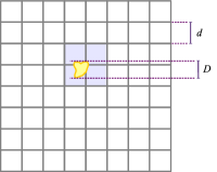
Figure 5: Placement of a secondary PM mesh (shaded) over a high-resolution particle region (yellow) such that an alignment with the underlying oct-tree geometry results. To determine the spatial extent of a commensurable secondary PM mesh, we first measure the maximum diameter $D$ of the high-resolution zone, which in turn is determined by the spatial positions of all particles of a designated particle type. Next, we compute the smallest power-of-two subdivision $d$ of the full box-size that is still larger than $D$. This identifies a fiducial regular Cartesian mesh with cell size $d$ covering the simulation domain, lining up with one level of the global oct-tree. All cells in this mesh that are touched by the high-resolution region become part of the region covered by the secondary PM mesh. The union of these cells is shrink-wrapped (imposing a cubical footprint) to determine the final extension and location of the secondary PM mesh.

GADGET-4 supports this in a similar spirit as GADGET-2, but with a number of improvements and changes. In practice, one or several particle types are designated to identify the spatial region where a PM calculation with a finer grid size is desired. The code automatically determines the smallest region enclosing these particles, and its maximum diameter $D$ in any of the principal axes directions. We then determine the size of the next larger node of size $d\geq D$ in the oct-tree covering the whole volume. The high-resolution region is now enlarged such that it lines up with the node boundaries in the corresponding level of the oct-tree, and has an overall cubical shape, as sketched in the example shown in Figure 5. Note that as a result, all tree nodes of this corresponding level of the tree as well as deeper ones (i.e. with smaller nodes) either fully overlap with the high-resolution region, or do not overlap at all. This is a feature we exploit in carrying out a clean force split that maintains manifest momentum conservation also in case a secondary PM mesh is used.

The enlarged high-resolution region is now covered with a secondary PM mesh, which is used to compute intermediate-scale forces for the mass contained within in it, using a zero-padded FFT to realize vacuum boundary conditions. The interaction kernel of this intermediate force is that of the short-range force corresponding to the coarse background mesh that covers the full box, minus the short-range force corresponding to the high-resolution mesh.

Forces for particles inside the high-resolution region are now computed as follows. Their total force is the sum of the ordinary background PM-mesh and the intermediate mesh force, augmented with a tree (or FMM) force that uses different short-range kernels depending on whether the interacting partner node is contained inside the high-res tree node, or whether it is outside. In the former case, the shorter interaction region $r_{\rm cut}^{\rm HR}$ of the high-res PM mesh is used, in the latter case, the more extended region $r_{\rm cut}^{\rm LR}$ of the background PM-mesh is used. For particles outside the high-resolution tree node, nothing changes compared to the plain TreePM or FMM-PM algorithms, i.e. their long-range force is simply the force of the background PM-mesh and their short-range force is computed with the normal, more extended cut-off $r_{\rm cut}^{\rm LR}$ for all other particles.

Note that in this tree algorithm there may never be an interaction of a particle inside the high-res region with a tree node that partly covers the high-res region, or in other words such nodes must always either fully contained or fully outside the high-res region. We achieve this because we geometrically align our high-res region with a level of the oct-tree, and we disallow interactions where a node partially overlaps with the geometric bounds of the high-res region, regardless of the opening criterion. Likewise, for the FMM algorithm, we only allow interactions between nodes that are either fully nested inside the high-res region, or lie fully outside. Effectively, this hence imposes an additional opening criterion according to which nodes that partly overlap with the high-resolution region are always opened. This allows interactions between any pair of particles where both are inside the high-res region to be treated with a sum of two PM forces and a short cut-off $r_{\rm cut}^{\rm HR}$ for the multipole expansions, whereas all other particle pairs are treated just with a single PM force and the corresponding background cut-off $r_{\rm cut}^{\rm LR}$. Note that this approach retains manifest force antisymmetry when FMM is used, because the PM algorithm itself also delivers antisymmetric forces.

Because we have $r_{\rm cut}^{\rm HR}<r_{\rm cut}^{\rm LR}$, the tree walks can be terminated earlier for the high-resolution particles when the secondary mesh is used, reducing the number of interactions that have to be evaluated for them. This constitutes the opportunity to speed up this part of the calculation. On the other hand, one needs to invest extra work for a further PM calculation, which due to the required zero-padding tends to be more expensive for a given grid resolution than the periodic FFT that can be used for the full box. And in the tree walk, we have to open extra nodes to avoid using nodes that overlap both with the high-res and the low-res regions. Whether or not this is worthwhile overall depends strongly on the particular setup encountered in practice. A minimum prerequisite for seeing a beneficial impact on the run-time is that the region that still needs to be covered by the tree walks around high-res particles, $(4\pi/3)(R_{\rm cut}r_{s})^{3}$, needs to be much smaller than the volume $(L^{\rm HR})^{3}$ of the full high-resolution region, otherwise substantial savings from being able to discard tree nodes can hardly be expected. Because of zero padding, the grid resolution is $d^{\rm HR}=2L^{\rm HR}/N_{\rm grid}^{\rm HR}$, so that this corresponds to the condition

$$N_{\rm grid}^{\rm HR}>>2\left(\frac{4\pi}{3}\right)^{1/3}A_{\rm smth}R_{\rm cut},$$ (37)

where $N_{\rm grid}^{\rm HR}$ is the full size (including zero padding) of the high-res PM mesh, and $r_{s}=A_{\rm smth}\,d^{\rm HR}$. Evidently, this tends to be easier to fulfil if one has a large problem size (which makes using a large $N_{\rm grid}^{\rm HR}$ worthwhile), and if one does not aim for very high accuracy (which means that a low value for $A_{\rm smth}$ is sufficient, as we will discuss later). We stress that this criterion provides only a rough indication for the regime in which a secondary mesh could in principle be beneficial.

We note that in contrast to the approach above, GADGET-2 required that the high-res particles interacted with all other particles using the short range kernel, which meant that the high-resolution PM-mesh needed to cover also a buffer region of size $r_{\rm cut}^{\rm LR}$ outside the designated high-res region. As for extreme zooms one can have $L_{\rm HR}<<r_{\rm cut}^{\rm LR}$, this meant that in this limit the effective extension of the high-resolution mesh was actually not determined any more by the size of the high-resolution region, limiting the dynamic range that could be bridged by the use of a single secondary mesh. In addition, not all interacting pairs of particles were treated symmetrically in this approach. Both disadvantages are eliminated by the refined procedure in GADGET-4. Another practical improvement is that the high-resolution region may now overlap with the periodic box boundaries in the initial conditions or during the evolution, which was previously not supported.

2.7 Gravitational softening

In collisionless dynamics, gravitational softening needs to be introduced to prevent the formation of bound particle pairs, and to protect against the occurrence of large forces and large angle deflections (which on top require short timesteps for proper orbit integration) when particles pass by close to each other. In practice, two questions have to be clarified in the force computation when individual softenings are assigned to particles and the potential is modified at short distance scales. First, how should the effective softening length of each interacting particle pair be obtained from the values assigned to the two particles? Second, how should the softening be treated in the tree algorithm, and in the calculation of the multipole expansions?

For the first question, we always adopt the conservative choice that the softening of any interacting pair of particles should be the larger of the two, i.e. we adopt

$$\epsilon_{ij}=\max(\epsilon_{i},\epsilon_{j}).$$ (38)

This preserves force antisymmetry and respects the idea that all interactions of a particle should be softened at least with the softening value assigned to it.

With respect to the second question, we store in the tree algorithm for each tree node the largest $\epsilon_{i}^{\rm max}$ and smallest softening $\epsilon_{i}^{\rm min}$ occurring among its constituent particles. In case the distance $r$ between a node and a particle (or a node and another node in the case of FMM) is larger than the maximum $\epsilon_{ij}=\max(\epsilon_{i}^{\rm max},\epsilon_{j}^{\rm max})$ of the largest softenings of the two nodes, the interaction is treated unsoftened, i.e. the multipole expansion is computed for the Newtonian interaction kernel. If the opposite is the case, we apply the softening $\epsilon_{ij}$ to the interaction of the two nodes, provided one can be certain that individual particles in the nodes are not treated with an excessively large softening because of this. In particular, one needs to protect against applying a softened multipole expansion to nodes with a mix of particles with different softening lengths, containing particle pairs between the nodes with smaller symmetrized softening than the node-level $\epsilon_{ij}$. This can only happen if both $\epsilon_{i}^{\rm min}<\epsilon_{ij}$ and $\epsilon_{j}^{\rm min}<\epsilon_{ij}$ are true. This is never the case for particle-particle interactions, and also not for interactions involving a node for which both $\epsilon^{\rm max}$ and $\epsilon^{\rm min}$ are equal to $\epsilon_{ij}$. Hence, if the conditions are not both true, we use the softened interaction, otherwise we proceed in the tree walk by opening the interaction.

In order to minimize the storage needs for $\epsilon_{i}^{\rm min}$ and $\epsilon_{i}^{\rm max}$ in the nodes as well as in the particle data itself, we use a discrete set of allowed softening values. Each particle then selects one of these softenings by being assigned a “softening class”, which is simply a one-byte value that indexes a global table with the available softening values. Correspondingly, only a single byte is needed for $\epsilon_{i}^{\rm min}$ and $\epsilon_{i}^{\rm max}$.

We note that in GADGET-3, softened interactions between cells and particles were never used and such nodes were always opened, i.e. softening was only allowed among particle pairs. However, this has the severe disadvantage that in regions where the particle density is high and the gravitational softening is comparable to the mean particle spacing, or if it is chosen deliberately much larger than this, the tree calculation locally degenerates to a $N^{2}$ behaviour and ends up computing a large number of two-particle pair-wise forces. In practical applications, this can happen, for example, in so-called zoom simulations when relatively large softenings are applied to heavy boundary particles, and those happen to contaminate the densely sampled high resolution regions. While our allowance for softened tree nodes alleviates this problem, it cannot eliminate it in all situations. For example, it is easy to see that mixing two particle types and assigning to one a considerably larger softening than the mean particle spacing can slow down the tree algorithm tremendously. If possible, it is thus advantageous to refrain from using very different softenings for particles that are spatially well mixed.

2.8 Periodicity only in two dimensions

A new feature in GADGET-4 is the option to have periodicity of gravity only in two spatial dimensions, while the third dimension remains non-periodic. This is intended mostly for simulations of stratified or shearing boxes that are frequently used to study small patches of the interstellar medium of disk galaxies at high resolution (e.g. Walch et al., 2015; Simpson et al., 2016). Self-gravity with periodic boundary conditions only in the directions parallel to the plane of the disk is needed in such simulations.

For this setup, an Ewald decomposition of the slowly converging potential sum can be derived (Grzybowski, Gwóźdź & Bródka, 2000), in the form

$$\psi({\bf r}) = \frac{1}{|{\bf r}|}+\frac{2\alpha}{\sqrt{\pi}}-\sum_{{\bf\tilde{p}}}\frac{{\rm erfc}(\alpha|{\bf r}-{\bf\tilde{p}}|)}{|{\bf r}-{\bf\tilde{p}}|}$$

$$-\frac{\pi}{L_{x}L_{y}}\sum_{{\bf k}\neq 0}\frac{\exp\left(i\,{\bf k}\cdot{\bf r}\right)}{|{\bf k}|}\left[\exp(kz)\,{\rm erfc}\left(\frac{k}{2\alpha}+\alpha z\right)\right.$$

$$\left.+\exp(-kz)\,{\rm erfc}\left(\frac{k}{2\alpha}-\alpha z\right)\right]$$

$$+\frac{2\sqrt{\pi}}{L_{x}L_{y}}\left(\frac{\exp(-\alpha^{2}z^{2})}{\alpha}+\sqrt{\pi}\,z\,{\rm erf}(\alpha z)\right),$$

where for definiteness we have assumed that the $z$-direction is the non-periodic dimension (our implementation is flexible in this regard). Here ${\bf r}=(x,y,z)$, and the sum over ${\bf\tilde{p}}$ extends only over the periodic replicas in the $x$- and $y$-dimensions. Similarly, the frequency integral over ${{\bf k}}$ extends only over the first two dimensions. We note that recently Wünsch et al. (2018) implemented a tree-based gravity solver with mixed boundary conditions in the FLASH (Fryxell et al., 2000) code. They derive an approximate expression for the potential of the mixed boundary case which differes from the analytic form above, but which appears to give sufficiently accurate results in practice.

Similarly to the ordinary periodic case, we calculate the force in the one-sided tree algorithm by taking account of the nearest periodic image in the $x-$ and $y$-directions with the ordinary Newtonian (softened) kernel, and by supplementing this with a correction force obtained from the above expression, evaluated through a Taylor expansion around the nearest point in a precomputed look-up table. Alternatively, we also support the TreePM and FMM-PM methods for mixed boundary conditions. Here the PM calculation is modified accordingly. In particular, we determine the Green’s function in Fourier space by first setting it up in real space with zero padding in the non-periodic dimension, and then transforming it to $k$-space.

2.9 Stretched boxes

Related to the above, we have generalized the gravitational algorithms of GADGET-4 such that they also support periodic boundary conditions for “stretched” boxes, i.e. the employed simulation domain does not have to be cubical in shape but may be stretched by different factors in each of the dimensions. This feature is not only available for periodicity in two dimensions as discussed above, but also for ordinary gravity with periodic boundary conditions in three dimensions. It works both for the one-sided Tree and for FMM, and also for TreePM and FMM-PM, respectively.

However, in the latter case, certain constraints for the stretch factors are enforced such that fully filled tree nodes remain cubical, and that there is an integer number of PM grid cells in each spatial dimension. The group finders and the hydrodynamical solver are operational for stretched boxed as well, but the placement of a secondary high-resolution PM mesh is not supported.

2.10 Integer coordinates

Ordinary floating point numbers are not ideal for representing the particle coordinates in our typical simulation setups, because they feature variable absolute positional accuracy throughout a simulation box (unless one restricts the numbers to specific factor of two ranges, for example by using the $[1,2]$ interval, such that the mantissa alone linearly encodes the position, as exploited in the Voronoi mesh construction algorithm of the AREPO code). Because our coordinates have bounded minimum and maximum values, at least a subset of the bits reserved for the floating point exponent are unused.

As an alternative it is attractive to consider integers for storing the coordinates in the box, as this delivers uniform resolution and can make optimum use of the bits assigned for the storage. When using 32-bit variables, the use of integers gives a relative positional accuracy within the box equal to $1/2^{32}\sim 2.33\times 10^{-10}$ instead of the machine precision of single precision floating point numbers, $\approx 10^{-7}$. This substantially enlarges the range of science applications where 32-bit values for the coordinates are sufficient. When double precision positions are replaced by 64-bit integer storage, the available relative accuracy in positional storage goes up to $5.42\times 10^{-20}$, enough to resolve Earth’s diameter in a box one Gigaparsec on a side, while for double precision floating point numbers it would be a thousand times worse.

A further advantage of integers is that it becomes particularly easy to determine both, a periodic mapping into the simulation box as well as finding the (signed) distance vector to the nearest periodic image of a point. Both just arise automatically without any branching in the code from the properties of the 2’s-complement used to represent signed integers, and the way integer overflows are treated on virtually all microprocessors used in high-performance computing. For example, imagine we use one unsigned byte to represent 256 possible positions along one periodic dimension of a simulation box. If a particle is at a position $x_{1}=200$ and another one at position $x_{2}=30$, then taking the distance of particle 1 relative to particle 2 one gets $x_{1}-x_{2}=170$, but interpreting the result as a signed integer, one gets $-86$, which is the distance of the nearest periodic image of $x_{1}$ to $x_{2}$ (which in principle lies at coordinate $200-256=-56$). Similarly, if we add a displacement to $x_{1}$, say a shift by $+100$ units, we do not obtain $300$ as new coordinate, but rather $44$ due to overflow – but this is exactly the correct coordinate we should get due to periodic wrap-around.

Integer coordinates also simplify the oct-tree construction, as they allow the use of fast bit-shift operations to determine in which (daughter) node a particle coordinate falls. The absence of numerical floating point round-off also eliminates any ambiguities in geometric predicates related to the tree construction. Likewise, the mapping onto Peano-Hilbert keys can be elegantly done in a ‘loss-less’ fashion due to the absence of floating-point integer conversions between coordinates and Peano-Hilbert keys.

For all these reasons, coordinates are internally stored as either 32-bit, 64-bit or even 128-bit integers in GADGET-4. Relative distances (i.e. coordinate differences) are first computed in integer and then converted to floating point values for subsequent calculations (such as determination of multipole moments). We also convert back to floating point values on input and output of particle data from initial conditions and snapshot files, respectively. A further possibility would be to reduce the number of significant bits that require storage by considering only the integer offset of a particle to a nearby neighbour, as proposed by Yu, Pen & Wang (2018). As we anyhow order the particles internally along a space-filling Peano-Hilbert curve, this could naturally allow a loss-less compression scheme that can substantially reduce the memory requirements for particle strorage. Yu, Pen & Wang (2018) also discuss how this idea can be extended to coarse meshes in velocity space. So far, such optimizations are not yet considered in GADGET-4, except for the possibility to use reduced precision in snapshot outputs for velocity data (half-precision format), and to apply loss-less compression to integer position data and particle IDs.

2.11 Non-periodic potentials

For simulations with non-periodic (vacuum) boundary conditions, the tree and FMM calculations simplify considerably, because mapping to nearest periodic images and Ewald corrections are not required. However, here the required size of the root node, which shrink wraps to the problem, may change during the system’s evolution. We determine the root-node automatically by shrink-wrapping the initial particle distribution, and by mapping it onto a subregion of our integer coordinates such that accidental nearest neighbour wrapping is avoided. Also, the code detects if a particle moves out of the boundaries of the original root node, in which case a new root node extension is determined.

Also in the isolated case, the Tree or FMM calculation can be combined with a PM acceleration for the long-range forces. In this case we implement non-periodic boundary conditions in the PM solver through zero-padding, i.e. the FFT size effectively used in each dimension is doubled relative to the periodic case. The Green’s function is set-up in real space, Fourier-transformed to obtain it in $k$-space, and then stored for subsequent use.

3 Force accuracy tests

basic algorithm	expansion order
	from dipole	to triakontadipole
just multipole expansion	Tree-O1	Tree-O5
	FMM-O1	FMM-O5
multipoles with mesh	Tree-PM-O1	Tree-PM-O5
	FMM-PM-O1	FMM-PM-O5
zoom runs: multipoles, mesh,	Tree-HRPM-O1	Tree-HRPM-O5
and additional high-resh mesh	FMM-HRPM-O1	FMM-HRPM-O5

Table 1: Overview of different gravitational force calculation algorithms supported in GADGET-4, wich are selected at compile-time. Tree and FMM designate that the hierarchical multipole calculation is done either with a classic one-sided Barnes & Hut tree code, or with a fast multipole method, respectively. These methods can be combined with a mesh covering the full simulation domain (PM schemes), where Fourier methods are used to accelerate the calculation of the long-range forces. For zoom simulations, it is possible to place a second mesh on a high-resolution region (HRPM schemes) that covers a fraction of the simulation domain where the particle density is particularly high. Each of these combinations can be run with different multipole expansion order, designated with O1 to O5, where the digits refer to the order parameter $p$. We also note that each of the methods can be run either with periodic or non-periodic boundary conditions, and with two different node opening criteria (a geometric opening angle, or our relative opening criterion). For periodic boundaries, also non-cubical domains are possible, but then the placing of an additional high-resolution mesh is not supported. Mixed boundary conditions with two dimensions periodic and one non-periodic are also supported, but in this case again a high-resolution mesh can not be used. In the older GADGET-2 and GADGET-3 codes, only the schemes Tree, Tree-PM and Tree-HRPM at order $p=2$ were available, while GADGET-1 only offered Tree-O3.

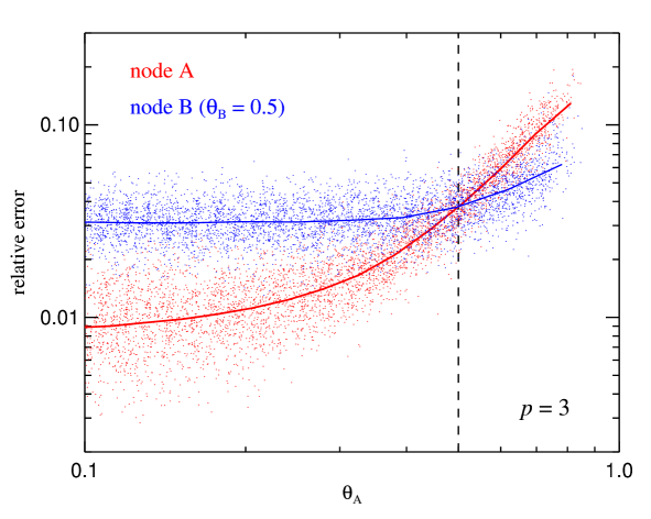
Figure 6: Relative force errors (individual points) and median force error (solid lines) for particles randomly distributed within two nodes if the interaction is computed with FMM (here for expansion order $p=3$), as a function of opening angle $\theta_{\rm A}$, for a fixed opening angle $\theta_{\rm B}=0.5$. Hence for $\theta_{\rm A}<0.5$, node A is smaller than node B, whereas for $\theta_{\rm A}>0.5$, node A is the larger of the two (the dashed vertical line indicates $\theta_{\rm A}=0.5$). The errors for the particles in node A are shown in red, while those for node B are in blue. For asymmetric node sizes, the smaller node experiences the smaller relative force errors.

The extensive discussion in the previous section shows that quite a number of different algorithms for the gravitational force calculation are available in GADGET-4. Table 1 provides a schematic overview of these methods. It is now important to test their accuracy systematically, and to establish how the force accuracy depends on the multipole order and other parameters of the chosen schemes. Once the basic force accuracy is verified, we can investigate the relative computational efficiency of the different methods. We are also interested in the important question of which algorithm delivers a given target accuracy with the smallest computational effort. Answering this question is non-trivial in general as it can be problem-size and machine dependent, but given the many choices that are possible in GADGET-4, it is important to develop at least a basic understanding of the performance implications of different algorithmic choices to facilitate the adoption of close to optimum settings in practical applications.

3.1 The FMM force accuracy between two interacting nodes

It is instructive to begin by considering the force approximation accuracy of the FMM approach for the interaction between two isolated cubical nodes as sketched in Figure 4. To this end we place 10 particles of equal mass randomly in each of two cubical nodes, which are themselves randomly placed with respect to each other, but with a certain distance $r$ between the resulting centers of mass of each node. We characterize the side lengths $l_{\rm A}$ and $l_{\rm B}$ of the two nodes through their respective opening angles as seen from the other node, i.e. $\theta_{\rm A}=l_{\rm A}/r$ and $\theta_{\rm B}=l_{\rm B}/r$. We then measure the force accuracy delivered by FMM for each of the particles in A due to those in B, and vice versa, for different opening angles and different multipole expansion order. For every realization of this setup, we determine the mean force error of the particles in each of the two nodes. To accumulate statistics, we repeat the random setup and the measurement many times over.

In Figure 6, we show the force accuracy for $p=3$ as a function of opening angle $\theta_{\rm A}$ for a fixed setting of $\theta_{\rm B}=0.5$, which effectively varies the sizes of the two nodes relative to each other. The results reveal several interesting trends (and they are qualitatively the same for different expansion orders $p$). For $\theta_{\rm A}<\theta_{\rm B}=0.5$, the node A is the smaller of the two, and its particles exhibit then also a smaller relative force error than those in the larger node B. For $\theta_{\rm A}>0.5$, the situation reverses, and now node B is smaller and has the smaller relative errors. We hence conclude that nodes should be of the same size in order to avoid an asymmetry in the induced relative force errors.

Also note that the relative force errors for node A asymptote to a value $\sim 0.009$ in the limit $\theta_{\rm A}\to 0$. This is because one then ends up seeing the effect of approximating the field created by node B with a finite multipole order $p$. Notice that this error is exactly the error one would get if the forces on particles in node A would be computed with an ordinary tree algorithm and node B is seen under an angle $\theta=0.5$. In the same limit of $\theta_{\rm A}\to 0$, the forces on the particles in node B also reach only a finite precision, even though node A now effectively shrinks to a point mass. This is because the resulting point mass field is still approximated within the volume of node B with a Taylor expansion, creating a finite error at the location of the particles within B. This type of error is absent in the ordinary tree algorithm. Importantly, it typically dominates the error budget in FMM, because it tends to be larger than the error induced by the source-side expansion.

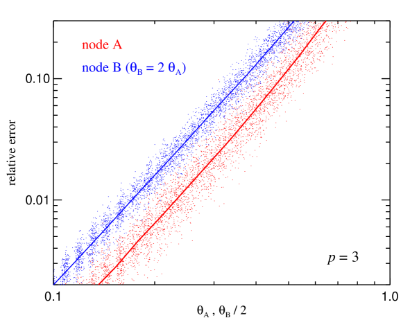
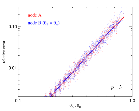
Figure 7: Relative force errors for particles randomly distributed within two nodes if the interaction is computed with FMM (for definiteness, with expansion order $p=3$), as a function of opening angles. Points show individual force errors, solid lines medians. In the top panel, node B is always chosen twice as large as node A (with results for B plotted also at the corresponding $\theta_{\rm A}$ value), whereas in the bottom panel, an equal node size is enforced. Only in the latter case, the relative force errors show a symmetric and equal distribution at given opening angle – apart from being smaller overall than for asymmetric node sizes.

The recommendation that equal node sizes are preferable is reinforced by the results of Figure 7, where we show in the top panel measurements of the force error scaling when one of the two nodes is twice the size of the other. Note that this situation would quite commonly arise when applying FMM to an oct-tree and always opening the larger of two nodes, as done in original algorithm by Dehnen (2000). While the force errors still scale as power-laws with $\theta^{p}$ in this case, they are highly asymmetric in their size distributions between the two nodes, which is undesirable. We therefore always open both nodes simultaneously in our FMM implementation if the opening criterion is triggered, guaranteeing a situation of equal node sizes whenever two nodes actually interact. The lower panel of Fig. 7 displays the corresponding error sizes in this case, which are symmetric and lowest overall for the given opening angle.

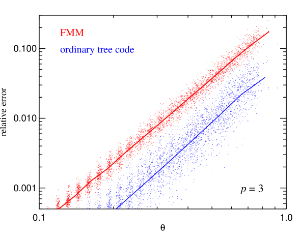
Figure 8: Relative force errors for particles randomly distributed within two equal-sized nodes as a function of the opening angle if the interaction is computed with FMM (red) or an ordinary tree (blue), here for expansion order $p=3$ (the results for different multipole order are qualitatively similar). Points show individual errors, while solid lines give medians. As expected, for equal expansion order and opening angle, the tree errors are lower than those of FMM because the latter needs to do an additional expansion at the sink side. However, the force errors for single node-node interactions scale with the same order in both approaches (i.e. the slopes of the solid lines are equal), as expected based on the truncation error of the underlying multipole expansion.

Having established that we prefer to always use $\theta_{\rm A}=\theta_{\rm B}$ for FMM in practice, it is interesting to compare the error sizes in this situation to those of the ordinary tree, as a function of the same opening angle. This is shown in Figure 8, for expansion order $p=3$ (other orders behave qualitatively very similarly). In both cases, the errors decline as power-laws with smaller opening angle, following the expected scalings based on the underlying Taylor expansion. The FMM error is however offset relative to the tree by an approximately constant factor of $\simeq 4$. This compares well to the difference in the error level seen in Fig. 6 for node A between $\theta_{\rm A}=0.5$ (i.e. the intersection of the two lines), and for $\theta_{\rm A}\to 0$. It corresponds to the accuracy price one pays in FMM for doing a Taylor expansion at the sink side as well. Of course, this loss of precision can be compensated for by using a correspondingly smaller value for the opening angle $\theta$ in FMM than for the tree code. In fact, based on these results, we would expect that $\theta_{\rm FMM}\simeq\theta_{\rm Tree}/2$ may deliver a comparable force accuracy for FMM and tree for $p=3$. But such a rule of thumb can be problem dependent, hence it is important to measure the achieved force accuracies for particle distributions that are of interest in practical applications. Note that our geometric opening criterion for FMM given in eqn. (35) will actually imply $\left<l/r\right>_{\rm FMM}\simeq\left<l/r\right>_{\rm Tree}/2$ for a prescribed numerical value of the maximum allowed opening $\theta_{c}$ in the code’s parameterfile, so the typical opening angles for FMM will automatically be smaller by a factor of 2 compared to the Tree, so that roughly comparable force accuracy should result for an unchanged setting of $\theta_{c}$.

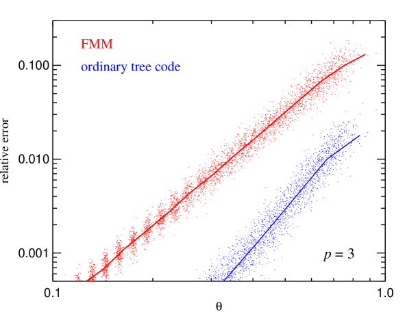
Figure 9: Relative force errors for the sum of the forces computed for 100 repeated calculations of the interaction of two equal sized nodes A and B, with randomly placed particles in them (and expansion order $p=3$, for definiteness). We consider only the force errors for particles in node A (with points marking individual particles, solid lines showing medians), which are kept fixed for the repetitions, whereas each time we replace the particles in node B with a newly drawn set of particles. In this experiment, the force errors measured for the tree are reduced compared to a single node-node interaction (compare with Fig. 8) due to a cancellation of force errors in different random directions. This effect is absent in FMM, because here the force errors are dominated by the sink-side expansion within node A, which stays equal in this experiment. For a full particle distribution, a given node will interact with a number of different nodes of similar size and at similar distance, akin to our set of 100 repeated realizations of a stationary node B, suggesting that cancellation effects of force errors should occur in more beneficial ways for the tree algorithm than for FMM.

In fact, depending on the particle distribution of an N-body system, FMM will often require an even more aggressive reduction of the opening angle in practice to exhibit a similar final force error as the tree algorithm. The reason for this is somewhat subtle and has to do with the way the force errors of different node-node (for FMM) or particle-node (for tree) interactions combine. As the total force on a particle in an N-body system arises from the sum of the forces of many multipole interactions, so does the total force error. If the individual force errors are all uncorrelated, they tend to average out in part. In particular, if one has $N$ similar partial forces pointing in a similar direction and making up the total force, each with uncorrelated relative force error, then the relative error for the total resulting force would see a $1/\sqrt{N}$ reduction compared with the relative errors in the partial forces.

We can check whether such an effect is present with a variant of our earlier node accuracy test. To this end, we repeat the computation of the forces for a given geometry and placement of nodes A and B a number of times (say 100 times), but each time we draw a new set of particles within B. We are then interested in the total force exerted on the particles in A (i.e. the sum of the forces of the 100 trials), and consider the corresponding force error. Figure 9 shows the result, comparing FMM and the Tree-based calculation. Comparing to the corresponding result shown in Fig. 8 for a single particle realization, we see that the force errors for the tree have gone indeed down significantly, by nearly a factor of 10 for small opening angles, as expected by a $1/\sqrt{N}$-scaling where $N$ is the number of forces that are added. In contrast, the FMM result for particles in node A has not changed, and no significant cancellation among the added force errors is seen. The reason is that the FMM force errors are dominated by the expansion on the sink side, and these errors are correlated with each other and are not random in direction, because a target particle in A has always the same location with respect to A’s center-of-mass. As we will see in the next section, this effect is present in realistic particle distributions as well, giving the tree algorithm an extra accuracy boost from cancellation of uncorrelated errors that is largely absent in FMM.

3.2 Force errors for an isolated particle distribution

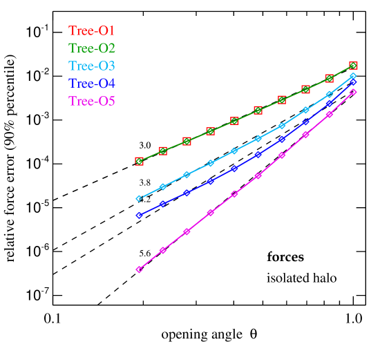
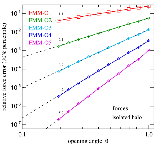
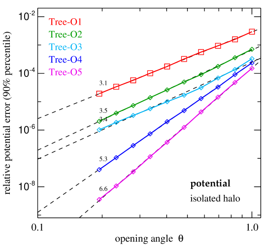
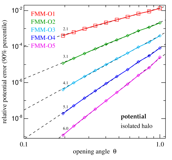
Figure 10: Characteristic force (top panels) and gravitational potential errors (bottom panels) as a function of opening angle $\theta$ for an isolated halo of 1 million particles, using the Tree and FMM algorithms in GADGET-4 at different multipole order, as labelled. Symbols mark our individual measurements for the 90 percentile errors, i.e. 90% of the particles have relative errors less than the quoted values. The scalings of the force and potential errors with opening angle are well described by power-laws. Fits to the individual measurements are given as dashed lines, and the values of the fitted logarithmic slopes are indicated in the different panels. FMM accurately follows the expected $\theta^{p+1}$ scaling of the potential error based on the leading order term truncated in the potential expansion, which translates to an expected $\theta^{p}$ scaling of the force errors. Similar scalings are obtained for the Tree algorithm, except that they are noticeably steeper than naively expected, an effect that we attribute to progressively larger cancellations of random errors as the interaction count increases towards smaller opening angles. For the tree algorithm, the orders $p=1$ and $p=2$ end up being equal for the force, due to the vanishing dipole moments and our convention for the acceleration expansion as given in equation (10).

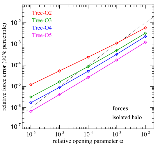
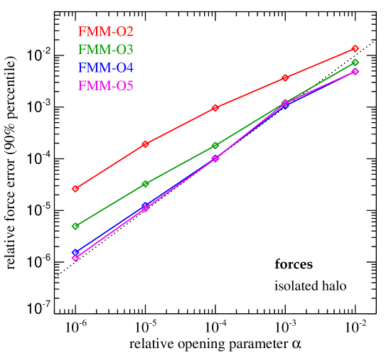
Figure 11: Characteristic force errors as a function of the relative opening parameter $\alpha$ for an isolated halo of 1 million particles, using the Tree and FMM algorithms at different expansion order $p$, as labelled. Note that for fixed $\alpha$, the force errors are of similar size when Tree or FMM are used, and they show only a weak residual dependence on multipole order $p$. This is the desired outcome, as this allows $\alpha$ to be used as a direct control of the desired force accuracy, approximately independent of the specific multipole algorithm that is chosen. The dotted line in the background gives the one-to-one relation between $\alpha$ and the 90% force error percentile, showing that this convenient behaviour is particularly well realized for FMM-O4 and FMM-O5. But note that the different methods may vary substantially in computational cost despite yielding similar final force errors.

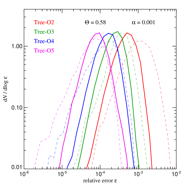
Figure 12: Distribution of the sizes of relative force errors for an isolated dark matter halo (1 million particles). In the left panel, we show results for the Tree algorithm, comparing the force error distributions for the relative opening criterion with fixed $\alpha=0.001$ at different expansion order $p$ (solid lines) with the corresponding force error distributions obtained for a fixed geometric opening angle $\theta=0.58$ (dashed lines). The right panel gives the corresponding results for the FMM algorithm. In both cases, we see that the geometric opening criterion produces a considerably broader error distribution than the relative criterion, and that its median error varies much more strongly with expansion order. Targeting an approximately constant force error is thus easier and more efficient with the relative criterion.

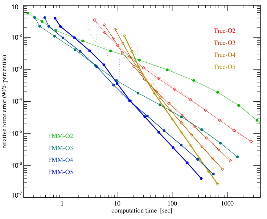
Figure 13: CPU time versus achieved force accuracy, comparing the Tree and FMM algorithms at different order $p$ for an isolated halo of 1 million particles, using the relative opening criterion. The geometric opening angle criterion always requires more computational time to reach a prescribed accuracy for a given order $p$ and algorithm, hence we omit to show results for it. In these tests, FMM is typically faster at the same accuracy than the Tree approach, except for FMM-O2, which becomes quite inefficient once a high force accuracy is requested. Which order $p$ is most efficient depends on the absolute value of the targeted force accuracy. If very high force accuracy is desired, it is always favourable to use high-order expansions, but if a lower accuracy is sufficient, this can eventually be computed in less time with a lower order scheme. This behavior is fairly general, but the exact transition points that delineate the regimes where different orders $p$ are optimal depend on details such as the clustering of the system under study, the boundary conditions, and the particle number. The measurements reported here are for an opening criterion where an exclusion region around every node (see Fig. 3) is not enforced for the one-sided tree, and interactions between neighbouring nodes in FMM are allowed. If our more conservative default node opening criterion is adopted, the code will not venture into regimes of very low force accuracy and exhibit a floor in execution time, with the corresponding results shown as thin dotted lines. The times reported here are for execution on a single core on an Intel Xeon Gold 6138 CPU at 2.0 GHz. We note that the relative contributions of the CPU time spent in different types of interactions is a function of the specific particle distribution, the order of the multipole expansion, and somewhat more weakly the force accuracy that is targetted. For example, for FMM-O5 in this test problem, around 27.0% of the computed interactions are particle-particle, 26.4% are particle-node, while 46.6% are node-node interactions. For FMM-O3, this shifts to 20.4% for particle-particle, 40.4% for particle-node, and 39.2% for node-node interactions. For assessing the relative CPU cost of these categories, one additionally needs to keep in mind that particle-particle interactions are always equally cheap, while interactions involving nodes become more expensive at higher multipole order.

We now consider force error measurements for the Tree and FMM algorithms for more realistic particle distributions. To this end we consider an isolated Hernquist (1990) halo consisting of 1 million particles and study the obtained force and potential accuracy when compared to exact results computed by direct summation for a random subset of the particles. In Figure 10, we show the errors for Tree and FMM algorithms as a function of opening angle $\theta$, and for different multipole expansion order $p$. In each case, we show the errors for the 90 percentile, i.e. a fraction of 0.9 of the particles has lower errors than given in the plots. Plotting median or mean errors instead yields qualitatively very similar results. We also include power-law fits to the measurements to highlight their scaling with opening angle.

Reassuringly, for Tree and FMM algorithms alike, the potential and force errors decline to good accuracy as power-laws with decreasing opening angle. The slopes reflect the leading order of the truncation error of the underlying Taylor expansions, as expected. However, the Tree-based errors decline noticeably faster in general than expected based on the multipole approximation error of a single node-particle interaction. Even when using only monopole moments in the force (this corresponds to $p=1$ and $p=2$, which are equal for the tree force as the dipole vanishes in our formulation), the error scales nearly as $\propto\theta^{3}$, and when quadrupole moments are included in the force ($p=3$), the scaling is $\propto\theta^{3.8}$. This can be understood as a consequence of the increasing interaction count with smaller opening angle, leading to more cancelation. For this particle distribution, the average number of multipole interactions per particle scales approximately as $\propto\theta^{-2.6}$ with opening angle. If all the partial forces were aligned, similar in size, and featured random errors of comparable size, we would expect to gain at most a steepening of 1.3 in the slope of the total force error scaling when the tree algorithm is used. In practice, we see a bit less, but still about $\sim 1.0$ for $p=2$, and slightly less for $p=3$. In contrast, little if anything of such a ‘cancellation-boost’ is seen for FMM, as we already anticipated based on our analysis of node-node interactions. This suggests that some of the speed advantage of FFM is eaten away by its less favorable behaviour with respect to error cancellations compared to the one-sided Tree method. We will return to the question of how CPU-time consumption as a function of achieved accuracy compares for different algorithms later on in this section.

The Tree-O3 result for the potential, and the Tree-O4 result for the forces, shown in Figure 10 look a bit peculiar. They noticeably deviate from a power-law and show a flatter scaling than expected based on the other results. We think this is because of the particular particle distribution examined here, where due to the spherical symmetry contributions sourced by the octupole moment are unusually small. Other, more irregular particle distributions show a much more regular run of this multipole order, confirming that this is a feature of the particular particle setup examined here.

In Figure 11, we show force error measurements for the same particle system, but this time as a function of the relative opening parameter $\alpha$. Again, we give measurements both for Tree and FMM, at different expansion order. It is reassuring that now the final force errors vary approximately in direct proportion to $\alpha$, and show only a comparatively weak dependence on the multipole order, or on whether the FMM or Tree method is used. This is the desired outcome for this opening criterion, which thus allows the use of $\alpha$ to conveniently set the desired force accuracy level, while the expansion order can be independently chosen according to performance considerations or memory use.

The relative opening criterion also affects the distribution of force errors, making them narrower in general. This is shown explicitly in Figure 12, where we give force error distributions for $\theta=0.58$ for both Tree and FMM for different expansion order $p$. This can be compared to corresponding error distributions obtained for $\alpha=0.001$. It is clearly seen that the medians of the force error distributions vary much less with expansion order when $\alpha$ is used, an effect that is particularly prominent for FMM. Also, the error distributions become narrower when $\alpha$ is used, particularly the low-force error tail of the geometric opening criterion is reduced. We also anticipate that this is reflected in a reduction of the computational cost at fixed median force error.

That this is indeed the case is becoming clear in Figure 13, where we now consider the force accuracy delivered by various ways to run the gravity solver against the CPU time invested. We show results both for Tree and FMM, for different expansion orders. As we find that the relative opening criterion is always more efficient than the geometric one, i.e. for fixed $p$ and algorithm, a given force accuracy is achieved with less computational time if the relative opening criterion is used, we only show results for the relative opening criterion in order to avoid making the plot overly busy. FMM is normally faster than the Tree approach, but there can be exceptions. For example, FMM-O2 is quite inefficient if a high force accuracy is targeted. In fact, for $p=2$ it would actually be better to use Tree-O2 in this regime. Note that the answer to the question which algorithm is the fastest depends on the desired force accuracy. For relative errors less than $10^{-4}$ this would be FMM-O5 (with the relative opening criterion), for errors between $10^{-4}$ and $10^{-3}$, it is FMM-O4, and for errors between $10^{-3}$ and $10^{-2}$ this is FMM-O3. If still larger errors are permissible, it could even be FMM-O2. This illustrates a general pattern that can also be observed for the results obtained with the Tree algorithm. Higher expansion orders become computationally worthwhile if high accuracy is demanded, but they are not necessarily the most cost effective if low accuracy is sufficient.

3.3 Force errors in periodic cosmological simulation boxes using Ewald corrections

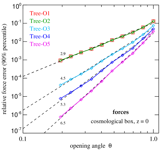
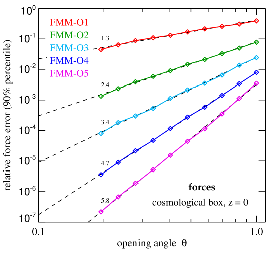
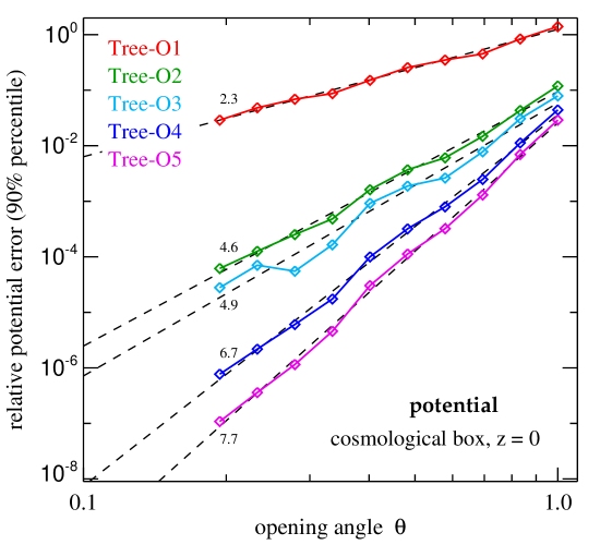
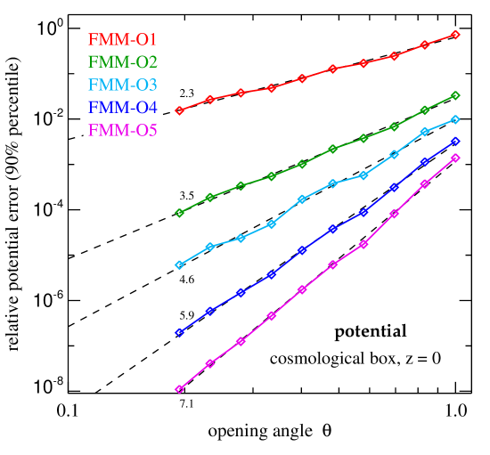
Figure 14: Relative gravitational force (top panels) and potential (bottom panels) errors as a function of the opening angle $\theta$ for a cosmological simulation box at redshift $z=0$ (using $128^{3}$ particles in a periodic box $30\,h^{-1}{\rm Mpc}$ on a side, with $5\,h^{-1}{\rm kpc}$ softening) using the Tree (left panels) and FMM algorithms (right panels), for different expansion orders as labelled. The scaling of the force and potential errors with opening angle is well described by power-laws (dashed lines); the values of the fitted slopes are inlined in the panels. The FMM approach follows the expected $\theta^{p+1}$ and $\theta^{p}$ scalings for potential and force errors quite accurately, whereas the Tree method performs typically somewhat better than expected due to progressively more relevant cancellations of random errors with increasing interaction count. Note that for our definition of the one-sided Tree algorithm, the $p=1$ and $p=2$ orders for the Tree-based acceleration are equal by construction.

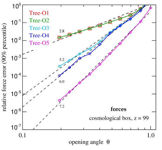
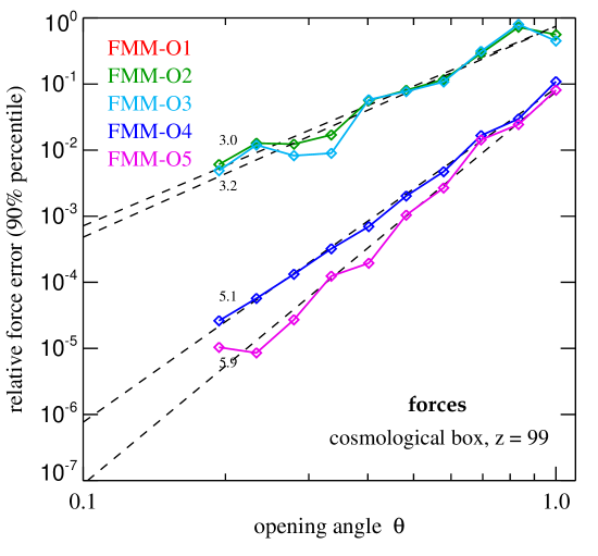
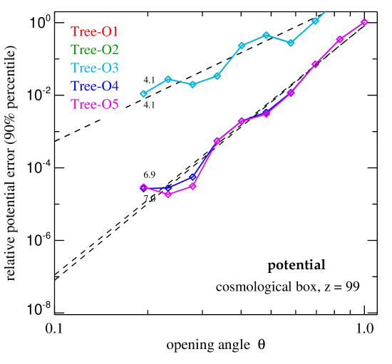
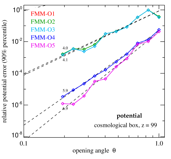
Figure 15: Characteristic force and potential errors as in Fig. 14, but now focusing on a cosmological simulation box at redshift $z=99$, where the particle distribution is nearly uniform and only slightly perturbed by the cosmological initial conditions. The scaling of the force and potential errors with opening angle is still reasonably well described by power-laws, although the values of the fitted slopes (as indicated in the panels) are less straightforward to understand, and the scalings feature some residual structure. The latter is presumably related to aliasing effects between the mildly perturbed Cartesian grid of particles, and the nested Cartesian oct-tree mesh used by the multi-pole expansions, causing relatively large discrete jumps in accuracy at certain opening angles. For the same reason, the octupole and triakontadipole moments of most tree nodes are expected to be very small, explaining why Tree-O2/O3 and Tree-O4/O5 are similar for the potential (in fact, Tree-O2 and Tree-O3 lie virtually on top of each other), and Tree-O3/O4 is very similar for the force. Likewise, the similarities of FMM-O2/O3 and FMM-O4/O5 are explained by these symmetry effects. We note that the accuracy of FMM-O1 for force and potential, and that of Tree-O1 for the potential, is so bad that the relative errors exceed unity and lie off-scale on the plots, hence these schemes are completely inadequate in the high redshift regime.

We now turn to the more demanding problem of accurately calculating N-body forces in a periodic space, which lends itself to a clean mathematical model of “infinite” space, giving a direct and accurate connection to linear perturbation theory, and thus to the standard formalism of large-scale structure theory. At high-redshift, the problem is particularly acute as here only small peculiar forces arise, which are the result of the addition of many forces from different matter perturbations on all scales. The small net force remains after cancellation of large forces in all directions, making this regime demanding for methods that work only in real space.

In Figure 14, we show measurements of the accuracy of force and potential values delivered by the Tree and FMM algorithms for different expansion order, as a function of the opening angle. The test system is here that of an evolved $z=0$ dark matter density field created by $128^{3}$ particles in a box of $100\,h^{-1}{\rm Mpc}$ across. This is thus representative of typical cosmic structure expected for $\sigma_{8}\simeq 0.85$ in today’s universe, at moderate mass resolution. We can see that both the Tree and FMM algorithms converge well towards the exact forces, which have here been computed with direct summation and Ewald correction for a random subset of the particles. As for the isolated halo, the Tree approach tends to converge with slightly steeper power-laws as the FMM method, a benefit that arises from more favourable error cancellation due to fewer correlations among the partial force errors. Also, we see that the forces for Tree orders $p=1$ and $p=2$ are identical, as expected. Only for $p=3$, the quadrupole moments of the tree nodes start affecting the forces.

The corresponding results for high redshift, $z=99$, which are representative for the epoch where normally initial conditions for such simulations are created, are shown in Figure 15. These results feature some interesting effects that look peculiar at first. First of all, the relative errors one obtains for a given opening angle are quite a bit larger at $z=99$ than at $z=0$. This reflects the small sizes of the peculiar potential and the peculiar forces for the only slightly perturbed density field at high redshift, which arises from the cancellation of large contributions to both quantities. This regime hence requires smaller opening angles for accurate results than needed for the highly clustered state at low redshift. Note that the accuracy delivered by Tree-O1 and FMM-O1 at high redshift (i.e. without PM mesh, as shown here) is particularly bad and essentially unusable for anything. This also holds true for the FMM-O1 force.

Another striking result of Fig. 15 is the fact that the potential for Tree-O3 is basically the same as that delivered by Tree-O2, and that the potential for Tree-O5 is almost the same as that for Tree-O4. This is also seen in a similar way for the FMM-algorithm. It appears that in this regime the addition of the octupole and triakontadipole moments is not really helping much. This is perhaps not too surprising, given that we use cubical nodes. If they can be approximated as nodes of uniform density, all uneven multipole modes vanish, and as Barnes & Hut (1989) has shown, even the quadrupole moment vanishes in this case exactly, making the hexadecupole moment the first non-trivial contribution. This is why we see a big jump in accuracy when this multipole moment is included in the potential calculation.

Another interesting effect is that the force accuracies of Tree-O3 and Tree-O4 are rather similar, while this is not the case for the FMM-algorithm. There the FMM-O3 rather lines up with FMM-O2, and not with FMM-O4. This is due to the importance of the sink-side expansion in FMM and its associated errors, which are absent in the Tree algorithm.

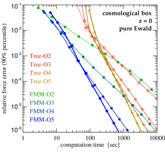
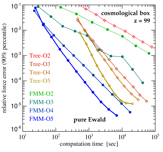
Figure 16: Force accuracy as a function of the invested computing time for our Tree and FMM algorithms when applied with different expansion order to a cosmological simulation with periodic boundary conditions, using Ewald summation. The particle number is $128^{3}$ with box-size $L=30\,h^{-1}{\rm Mpc}$ and $5\,h^{-1}{\rm kpc}$ softening, as in Figures 14 and 15. The left panel shows results for the evolved density field at $z=0$, while the right panel is for the initial conditions at $z=99$, which are more demanding to calculate in real space due to the small peculiar forces at that time (note the change in range on the $x$-axes in the two panels). The solid lines give results for different settings of our relative opening criterion; the geometric opening criterion is not shown for clarity as it always has a worse performance (particularly at low redshift, while at high redshift it is nearly on par). The reported times are for execution on a single processor core, and for the use of Ewald correction in all interactions to correct for periodic boundary conditions. Thin dotted lines give equivalent results when our conservative near-node exclusion zone around every tree node is enabled, which otherwise has not been used in the results reported as solid lines. The higher order schemes, in particularly for FMM, are generally the most efficient, with few exceptions at low force accuracy.

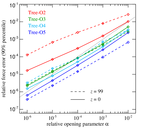
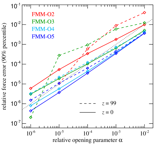
Figure 17: Force accuracy as a function of the relative opening parameter $\alpha$ for cosmological simulation boxes, shown both for the Tree (left panel) and FMM (right panel) algorithms. In each case, we compare results for $z=99$ (dashed) with those obtained for the clustered state at $z=0$ (solid), for different expansion order. The dotted line in the background gives a one-to-one relation between $\alpha$ and the 90% force accuracy percentile, which may also serve as a reference for comparing Tree and FMM with each other. Reassuringly, the measured force accuracies for fixed $\alpha$ are reasonably independent of the employed algorithm, the expansion order, and the clustering state of the particles, especially so if one refrains from using the lower orders. This means that the parameter $\alpha$ of the relative opening criterion can used as a convenient and reliable control of the desired relative force accuracy throughout the course of a cosmological simulation.

In Figure 16, we compare the relative computational efficiencies of these schemes with each other by now looking at the achieved force accuracy as a function of consumed CPU time. We again focus on results for the relative opening criterion as this is always at least as efficient as the geometric one. Note that here all interactions are Ewald-corrected, which makes them notably more expensive than for non-periodic boundaries. But at least for the clustered state at $z=0$, the relative efficiencies of the different schemes closely resemble the results shown in Fig. 13 for an isolated halo. At the high redshift of $z=99$, we see however that the calculations become much more expensive. Through the use of the relative criterion a roughly constant force accuracy for specified opening parameter $\alpha$ is maintained independent of clustering state, something that we demonstrate explicitly in Figure 17. To reach the same small relative force error at high redshift with a pure multipole-based approach thus requires more nodes to be opened, and hence a more costly calculation. Interestingly, in this regime especially the low-order schemes struggle substantially, and it really pays off to use one of the higher-order methods, particularly FMM-O5 looks attractive if relative errors of $10^{-3}$ or smaller are desired with a pure real-space method at high redshift.

3.4 Effective force law for Tree-PM and FMM-PM

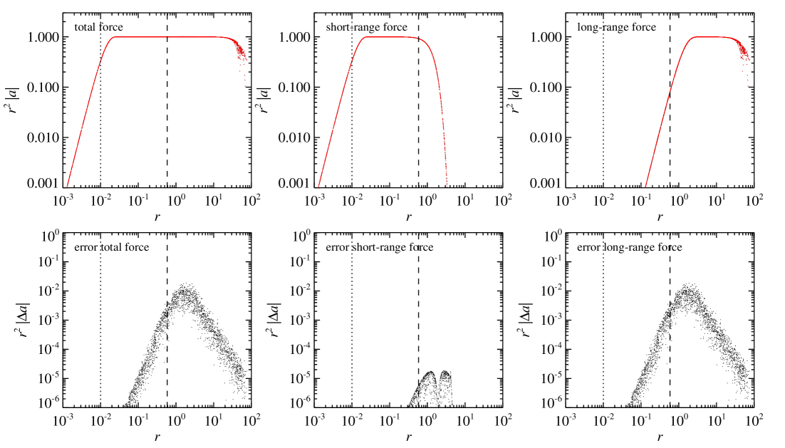
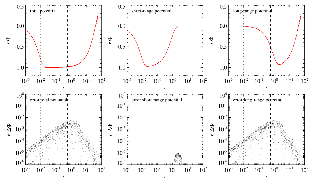
Figure 18: Force and potential laws arising in GADGET-4’s TreePM and FMM-PM approaches to compute the total force as a sum of a short-range force delivered by a Tree- or FMM-approach, and a long-range force computed with a PM-method. The forces and potentials in this test are computed by placing a point particle of unit mass randomly into a periodic box and by choosing random evaluation coordinates. Note that for this setup, the results for Tree-PM and FMM-PM are identical by construction. The box size is $100\,h^{-1}{\rm Mpc}$, with $r$ given in units of $h^{-1}{\rm Mpc}$. In the top row of panels, we show the total force (top left) as a function of distance to the point mass, and decomposed into the short-range (top middle) and long-range (top right) components. In the three cases, the force has been multiplied by $r^{2}$ to highlight deviations from a Newtonian force (which corresponds to a horizontal line in these panels). The increase for small $r$ reflects the gravitational softening law (of size $\epsilon=10\,h^{-1}{\rm kpc}$, marked by dotted lines), while the decline and scatter at large $r$ are due to the periodic boundary conditions (see also Fig. 2). In the second row of panels, we show the relative force error arising in this approach, again as a function of distance from the point source and separately for the total force, and its short-range and long-range components. The short-range force error is higher than machine precision in the force matching region, due to our use of a look-up table to avoid costly evaluations of complementary error functions. However, the associated error is generally much smaller than the finite error of the PM approach itself, which originates from the use of a finite grid size (here $N_{\rm grid}=256$) and grid smoothing scale (here determined by $A_{\rm smth}=1.5$, yielding $r_{s}=A_{\rm smth}L_{\rm box}/N_{\rm grid}=0.59\,h^{-1}{\rm Mpc}$ marked by dashed lines), from CIC binning and interpolation, as well as from finite differencing to get the force from the potential. Hence, in the limit of small tree opening angle, the total error is dominated by the PM-force, and peaks at the force matching scale. Similarly, the third and fourth rows show the corresponding decomposition of the total gravitational potential of a point mass into short-range and long-range contributions (here multiplied by $r$ to compress the vertical dynamic range), and the corresponding relative errors, respectively. Note that the total peculiar potential becomes positive at separations that approach half the box-size.

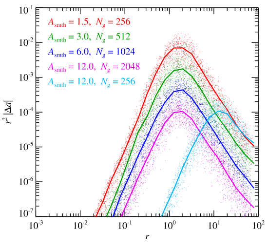
Figure 19: Relative force error for a point mass as a function of distance in the TreePM or FMM-PM schemes, for different choices of PM-mesh size $N_{\rm grid}$ and grid smoothing parameter $A_{\rm smth}$, as labelled. The maximum error occurs at the force matching scale, and is originating in the PM force. It can be arbitrarily reduced in size for fixed force matching scale by increasing $N_{\rm grid}$ and $A_{\rm smth}$ in lock-step. If only $A_{\rm smth}$ is increased, the error declines as well, but then the force matching scale becomes larger, such that the Tree or FMM calculations of the short-range force need to cover a larger volume and thus become more expensive.

As described in Section 2, an alternative approach to treat periodic boundaries is obtained by combining the Tree or FMM methods with a PM-based calculation. We begin by examining the basic force law of the code for different scenarios in this case, in particular to study the importance of the force matching region in this case. In Figure 18 we show the effective force law delivered by the code for a randomly placed point mass of unit mass within a periodic box of size $L=100$ in dimensionless units, with $G=1$. We compare the forces obtained by the short-range tree and the long-range PM calculations with the exact forces for the corresponding parts, determined by evaluating the relevant Ewald sums with high precision.

The decline of the force for small $r$ shows the effect of the gravitational softening, whereas the flat part in the top left panel corresponds to the $\sim 1/r^{2}$ regime of the force. Once the distance reaches an appreciable fraction of the box-size, the force law deviates noticeably from this, with the force dropping to zero at a distance approaching half the box-size. Likewise, the peculiar potential changes sign and becomes positive in this regime.

Note that if the softening length $\epsilon_{0}$ exceeds about $1.75\,r_{s}$, the short range force becomes repulsive as it then needs to compensate the excess PM force which is computed disregarding the softening length. Running the code in this mode is not very efficient, as $r_{\rm cut}$ then needs to be made relatively large (recall that $r_{\rm cut}$ should be larger than $2.8\,\epsilon_{0}$). But if instructed to do so, GADGET-4 can still be operated in this regime.

We see from Fig. 18 that the total error of the force and the potential due to the Tree-PM/FMM-PM approach is generally very small, except at around the force matching scale, where in this example the relative errors reach a maximum of around 1%. There are two sources for these errors. In the short-range force, they can arise from interpolation errors in the look-up table we use to avoid expensive evaluations of complementary error functions, or from the use of a too small value of $r_{\rm cut}$ that causes distant contributions in the short-range force to be neglected. In the long-range force, the force errors arise from residual anisotropies of the PM-force and from truncating the Fourier series at some finite Nyquist frequency.

These errors can be reduced easily, essentially arbitrarily. In the former case this can be done by using a finer look-up table and/or a larger $r_{\rm cut}$, in the latter case by enlarging $A_{\rm smth}$. Our short-range look-up table has a default length of 48 entries out to $R_{\rm cut}$. Making the table finer reduces the achievable short-range force errors, but this is pointless unless the residual PM error is reduced to a similar or smaller level. The PM-force error on the other hand reflects the residual discreteness and finite size of the grid used for this part of the calculation. The size of the corresponding errors can be reduced, if desired, by resolving the PM force with more cells (or in part by using higher-order kernels, such as TSC instead of CIC), i.e. keeping the transition scale $r_{s}$ fixed but using a finer PM-mesh, which effectively means to increase the grid size $N_{\rm grid}$ and the parameter $A_{\rm smth}$ in lock-step. One may also increase $A_{\rm smth}$ alone without increasing the PM-mesh size itself. This will also reduce the maximum error of the PM-force while keeping its computational cost constant, but now the short-range force becomes more expensive as then $r_{s}$ grows and fewer tree nodes can be discarded. Note however that there is a limit to all this, dictated by the requirement that we should see only one nearest neighbour within the short-range cut-off region, otherwise the Tree-PM or FMM-PM approach will break down. If we conservatively set $r_{\rm cut}=8\,r_{s}$, this translates to the important condition $A_{\rm smth}<N_{\rm grid}/16$.

In Figure 19 we show how the maximum long-range force error varies with the chosen $A_{\rm smth}$ and the mesh size. Changing from $A_{\rm smth}=1.5$ to a much more conservative value of $A_{\rm smth}=12.0$ reduces the maximum error by about two orders of magnitude, to a level of $10^{-4}$. Provided one stays within the constraint $A_{\rm smth}<N_{\rm grid}/16$, this maximum error is then independent of the grid-size itself.

3.5 Force accuracy for the Tree-PM and FMM-PM approaches

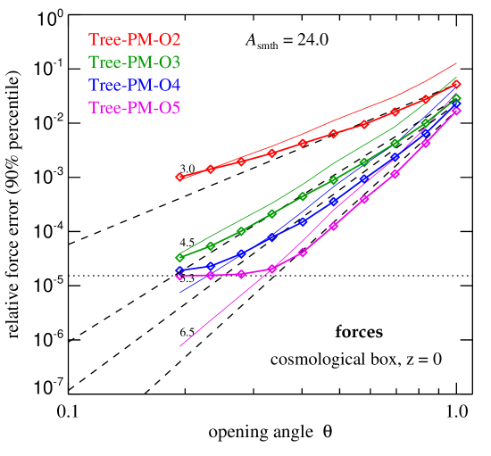
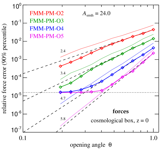
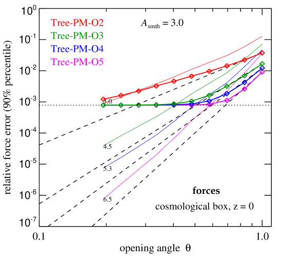
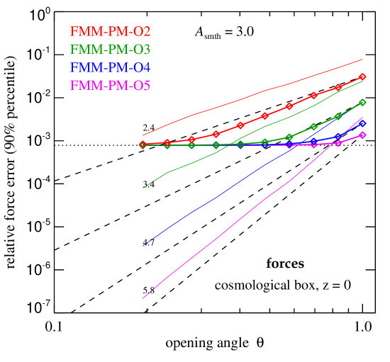
Figure 20: Force accuracy as a function of geometric opening angle $\theta$ for a cosmological simulation box at $z=0$ when the Tree-PM (left column) or FMM-PM (right column) algorithms are used with different expansion orders, and for different choices of the grid smoothing parameter $A_{\rm smth}$. In the top panels, a comparatively large force-split scale corresponding to $A_{\rm smth}=24$ with $N_{\rm grid}=512$ has been used, while the two bottom panels used $A_{\rm smth}=3$ with $N_{\rm grid}=256$, i.e. a four times smaller split scale. The examined particle distribution is the same as used in Figure 14, where equivalent results for pure multipole expansions with Ewald correction were shown. In fact, these former results are here repeated as thin solid lines, for easier comparison with the results obtained for the Tree-PM and FMM-PM algorithms, which are shown with thick solid lines. The dashed lines show the power-law scalings inferred from these pure multipole results, but normalized to the errors obtained for the Tree-PM or FMM-PM methods for $\theta=1$. For large $\theta$, the errors are actually slightly reduced when the PM approach is enabled, due to the more accurate computation of the long-range force components this entails. In this regime, the errors are then dominated by the short-range force, and decline towards smaller opening angle as expected for the corresponding multipole order. However, the errors eventually hit an irreducible floor (marked by dotted horizontal lines), which originates in the finite accuracy of the PM calculation. Further reducing $\theta$ is futile in this case, but increasing $A_{\rm smth}$ can make the total error still smaller, if desired.

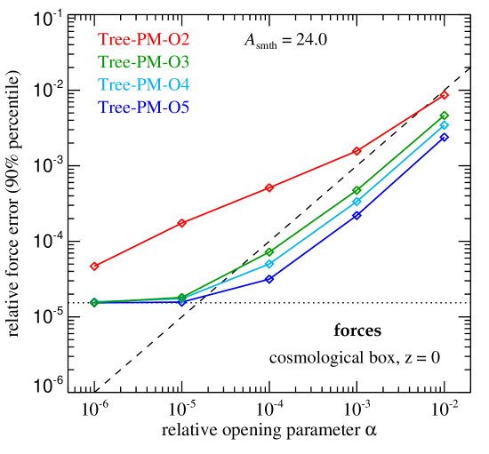
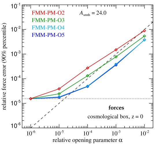
Figure 21: Force accuracy for a cosmological simulation box at $z=0$ when the Tree-PM (left panel) or FMM-PM (right panel) algorithms are used with the relative opening criterion, for different multipole orders $p$. The diagonal dashed line has a slope of unity and corresponds to a one-to-one relation between the opening parameter $\alpha$ and the 90-percentile force error. This line is followed reasonably well for large values of $\alpha$, to good accuracy independent of multipole order and multipole scheme. In this regime, the force errors are dominated by the tree-based component. Similarly to the approach with Ewald-correction, one can thus use $\alpha$ to directly set the desired force accuracy level. However, for small settings of $\alpha$, a floor in the force accuracy (dotted line) is reached which is set by the finite precision of the PM force (see also Fig. 20). In this case, a further improvement of the relative force error can not be reached by reducing $\alpha$; instead it requires a reduction of the force error from the PM computation by increasing $A_{\rm smth}$.

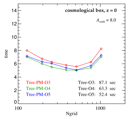
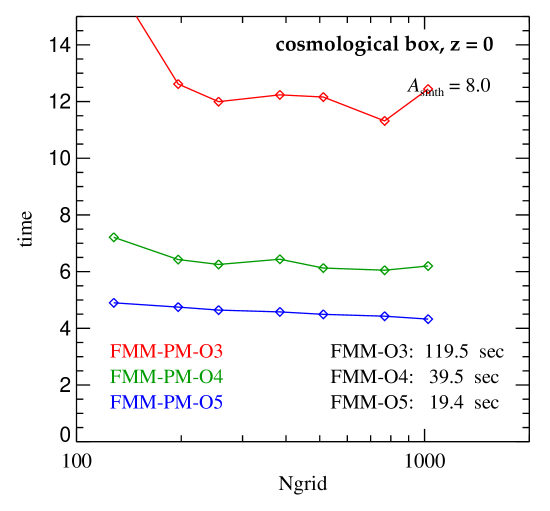
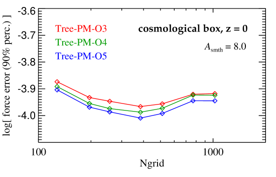
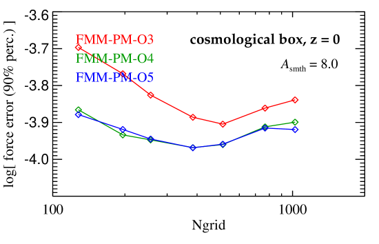
Figure 22: Force calculation time and force accuracy in the Tree-PM and FMM-PM algorithms as a function of the mesh size employed. We here adopt a constant value of $\alpha$ (for definiteness chosen conservatively as $\alpha=0.0001$, and with a high $A_{\rm smth}=8.0$ to suppress PM force errors to correspondingly low levels), but vary the grid resolution $N_{\rm grid}$ over a wide range. In particular, we would like to establish whether the execution time depends strongly on $N_{\rm grid}$. The panels on top thus show the runtime for a full force evaluation of a $128^{3}$ run at $z=99$ in a $30\,h^{-1}{\rm Mpc}$ box, carried out with $N_{\rm cpu}=40$ cores for different $N_{\rm grid}$, with the TreePM algorithm on the left, and the FMM-PM on the right. Coloured lines give results for different multipole expansion orders, as labelled. Reassuringly, the force accuracy shows only negligible variation for different mesh choices, and also Tree-PM and FMM-PM are quite similar overall. The bottom panel shows the corresponding force accuracy measurements. With respect to run-time, CPU-time consumption is shifted from the tree-based calculations to the Fourier-based computations for growing $N_{\rm grid}$, but their sum varies only comparatively weakly with $N_{\rm grid}$. There is an optimum for a grid resolution about $2-3$ times the particle grid, and this is somewhat more pronounced for TreePM compared to FMM-PM. Interestingly, FMM-PM on the other hand shows a stronger sensitivity of its runtime to expansion order (note that this is at fixed force accuracy). Clearly, only for high order our FMM-PM implementation begins to (moderately) outperform Tree-PM. Note that if the multipole methods are however run without the PM-acceleration for the periodic box, they are indeed quite a bit slower; this is demonstrated by the inlined numbers in the top panels, which give the corresponding execution times if the Tree or FMM methods are used, which have to rely on Ewald correction instead.

We now repeat our measurements of the force accuracy in cosmological boxes, but this time employing combinations of the PM algorithm with the Tree or FMM methods. In Figure 20, we show results for the same $z=0$ dataset considered earlier, this time employing either Tree-PM or FMM-PM methods for different expansion order. We also consider the PM algorithm for two different values of $A_{\rm smth}$. In general, we see that for large opening angles, Tree-PM and FMM-PM show slightly better accuracy than the corresponding pure multipole algorithms, whereas for small opening angle, the accuracy asymptotes to a finite value that can not be improved any further by reducing the opening angle. Clearly, in this regime the accuracy is limited by the PM part of the algorithm, and improving it further requires increasing $A_{\rm smth}$.

In contrast, in the opposite regime, for large opening angles, the accuracy is limited by the short-range Tree and FMM parts, respectively. Here the errors scale with the same power-law as in the plain multipole algorithms, but the amplitudes are a bit smaller because part of the force is supplied by the (in this regime) more accurate PM computation.

This raises the question which settings are optimal as far as the computational cost of the Tree-PM and FMM-PM algorithms is concerned. For a fixed split scale $r_{s}$, the optimum will be reached if the contribution to the force errors of PM and Tree/FMM are roughly equal. Because if the PM was more accurate than the Tree/FMM, one could typically save computational time by using a smaller $N_{\rm grid}$, combined with a smaller $A_{\rm smth}$ at fixed $r_{s}$. This would leave the Tree/FMM errors invariant and increase the PM error, but since the former dominates, the final result would not change significantly. Conversely, if the Tree/FMM part would produce subdominant errors, one could increase the opening angle while saving CPU time until the errors of both force components are roughly equal. What is not immediately clear, however, is which value of $r_{s}$ is best for a given problem.

In Figure 21 we first verify that the relative opening criterion still roughly works in TreePM/FMM-PM as a convenient way to set the overall relative force accuracy of the multipole part of the force, independent of expansion order. A simple strategy for finding the optimum run-time regime can then be as follows. One first decides about the desired force accuracy level, and then sets $A_{\rm smth}$ to the smallest value such that this can be reached. Likewise, one uses a corresponding $\alpha$ value. One can now vary $N_{\rm grid}$ systematically, subject to the constraint $N_{\rm grid}>16\,A_{\rm smth}$, picking the value that minimizes the runtime for a given expansion order $p$. Of course, the optimum thus identified will in general depend on the particular system that is studied, on details of how the algorithm is actually coded up, whether or not single precision is used in parts of the calculations, how large possible parallelization losses are, and on technical details of the platform that is used to execute the test. But the qualitative findings should be robust to these details, and thus can ideally allow the identification of general recommendations that then lead to practical settings that are not too far away from optimum ones.

Figure 22 provide some pointers along these lines. We here examine how the performance of the Tree-PM and FMM-PM schemes varies as a function of the chosen mesh size, at approximately fixed force error. Interestingly, we find that the optimum is fairly broad as a function of $N_{\rm grid}$, i.e. provided one choses $N_{\rm grid}\sim(2\pm 1)\,N_{p}$, where $N_{p}^{3}$ is the particle number, the PM-accelerated multipole algorithms give good performance. We also find that going to high order tends to be more important for FMM than for the one-sided Tree in order to reach the highest speeds. Interestingly, FMM-PM however does not show a clear speed-advantage over Tree-PM, unlike the case for plain FMM vs. plain Tree. There appears to be even a slight advantage for TreePM, except for order $p=5$, where FMM-PM-O5 comes out narrowly on top. In the figure, we also report the times taken for the plain multipole algorithms when applied with Ewald correction to the same problem. They show that the hybrid PM approaches are considerably faster than the plain multipole algorithms with Ewald summation, hence for cosmological simulations, Tree-PM and FMM-PM are the most efficient solvers in GADGET-4.

3.6 Secondary Fourier mesh for a high-resolution zoom region

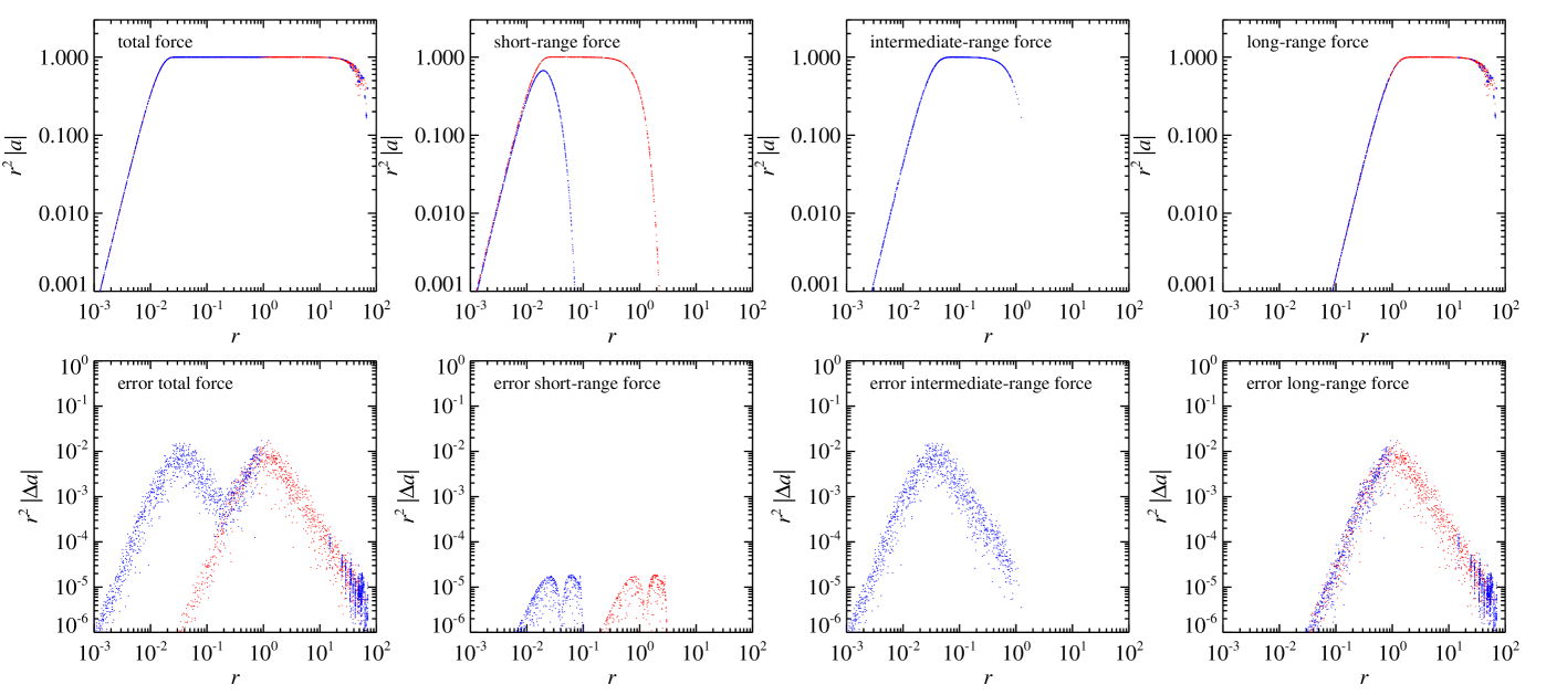
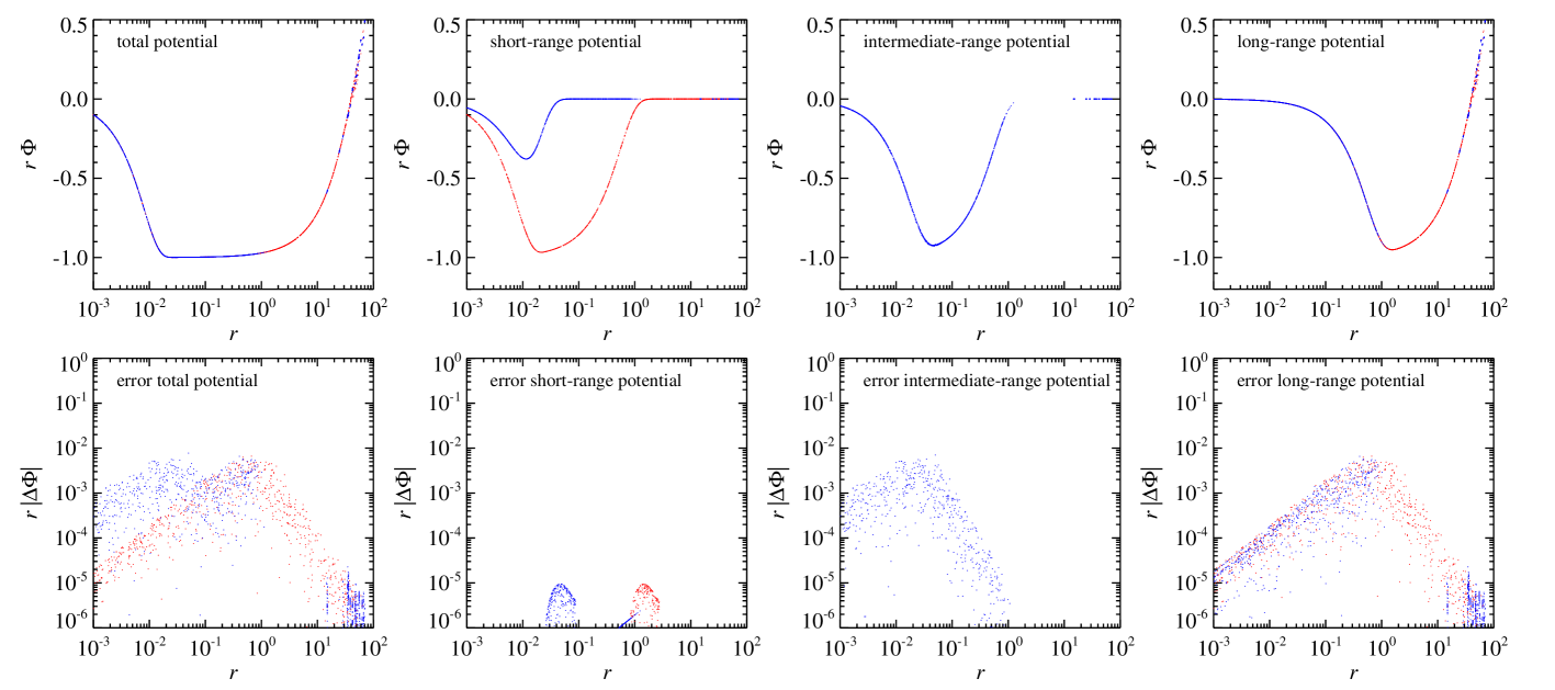
Figure 23: Force and potential laws resulting from GADGET-4’s Tree-HRPM or FMM-HRPM approaches, where a secondary high-resolution PM mesh is used to accelerate the force calculation in cosmological ‘zoom’ simulations. This plot is similar to Fig. 18, except that here also a secondary high-resolution PM mesh is present. Whether or not the force between two particles is computed with the ordinary Tree/FMM-PM approach, or with one where two Fourier meshes are used, depends on the spatial locations of the particle pair. If both of them are inside a cubical high-resolution region (which includes all particles of a certain pre-defined type), then a secondary force-split scale is introduced in the short-range part of the usual Tree/FMM-PM method, so that the region that is computed with the multipole approach shrinks further, and a secondary PM mesh (with zero-padding to realize non-periodic boundary conditions) can be used to complement the force with an intermediate-range contribution. In the present plots, particles where this applies are plotted in blue. If at least one particle of a pair is outside the high-resolution region, no secondary PM mesh is used and only the single split scale of the ordinary Tree/FMM-PM approach applies. These are the red particles in the plots. For the short-range force, there are thus two different force and potential laws for blue and red particles. The intermediate-range force is only relevant for blue particles, while the long-range force law applies to both in the same way. The largest errors in this approach occur in the two force matching regions and originate in the finite accuracy of the PM approach. The latter can however be made more accurate, if desired, by using an appropriately larger smoothing $A_{\rm smth}$ and mesh size $N_{\rm g}$. Note that the number of cells per dimension for the background PM mesh covering the full box and for the high-resolution patch can in principle be chosen independently.

In Figure 23, we extend the previous test to the case of an active high-resolution placement. First we show the effective force law for an illustrative test case where the high-res region covers 1/10 of the periodic box. Again, we place a source particle randomly inside the box, sometimes inside and sometimes outside the region covered by the secondary high-resolution PM grid, and then measure the force accuracy delivered by the code relative to the analytic expectation. This in particular allows us to characterize the force accuracy in the transition regions between the PM meshes and the short-range tree force. Recall that the high-res patch is aligned with the geometry of the oct-tree at a suitable grid level.

Similar to the ordinary TreePM and FMM-PM schemes with just a single, periodic FFT, we obtain for $A_{\rm smth}=1.5$ a total force error that is of order 1% error in the force matching regions. If desired, this force error can be reduced by using a larger value for $A_{\rm smth}$. For a fixed PM-mesh size, this however means a larger $r_{s}$ and thus more work for the Tree or FMM algorithm.

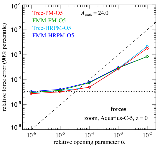
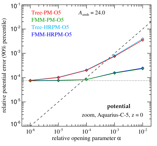
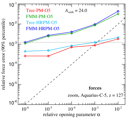
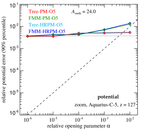
Figure 24: Test of the force and potential accuracy for a typical zoom simulation setup, calculated with the Tree-PM and FMM-PM approaches, both with and without the placement of a secondary high-resolution Fourier mesh. The initial conditions and the evolved simulation correspond to the run Aq-C-5 of the Aquarius project (Springel et al., 2008a). We show results as a function of the specified relative opening parameter $\alpha$, and restrict ourselves here to order $p=5$ for simplicity. Other expansion orders look qualitatively very similar, but may differ more significantly in run time. The top panels give results for $z=0$, the bottom ones for the initial conditions at $z=127$, with force accuracy shown on the left and potential accuracy on the right. A setting of $A_{\rm smth}=24.0$ for high accuracy of the PM-mesh calculations is used, allowing the code to deliver small relative errors despite the complicated force and potential matching entailed in Tree-PM and FMM-PM, respectively. At high redshift, it is comparatively difficult to get very low relative force and potential errors, not only because of the smallness of the force and potential values, but also due to the rapid coarsening of the sampling of the boundary region and the associated drastic increase of the particle masses, making this a more challenging set-up than for uniform sampling. In all cases, enabling a secondary PM mesh hardly changes the accuracy of the final results, as desired. Bot the Tree and FMM methods deliver very similar accuracy, and this is effectively set by $\alpha$ in the low-accuracy regime (approximately following the dashed line), while for low $\alpha$ the accuracy is limited by the PM-approach (horizontal dotted lines).

In Figure 24 we show results comparing the accuracy for different combinations of Tree-PM and Tree-HRPM, as well as FMM-PM and FMM-HRPM. For conciseness, we here restrict ourselves to order $p=5$, and go for relatively high accuracy facilitated by a setting of $A_{\rm smth}=10^{-5}$. Results for other orders or lower values of $A_{\rm smth}$ look as expected based on our other earlier tests.

3.7 Force error distributions for mixed boundary conditions

The variety of different force computation algorithms in GADGET-4 that we have discussed thus far is further extended by algorithms that employ stretched periodic boxes, or (stretched) boxes in which only two dimensions are treated with periodic boundaries, while the third has open boundaries. It is of course important to check the typical force accuracies delivered by the code in these situations as well. We have done this in a dedicated suite of test calculations, but refrain from going through all the combinations here in the interest of brevity, because the results are qualitatively very similar to what we have discussed thus far. We will however come back to the problem of a stretched tall box in one of our example problems later on.

3.8 Correlated force errors

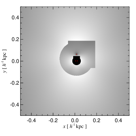
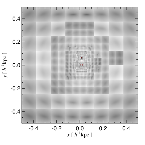
Figure 25: Maps of the relative force error in the $xy$-plane (encoded in grey-scale) for a distribution of three equal point masses. The points are located at the coordinates marked with red dots in the maps. The panel on the left gives the error map for a one-sided tree algorithm, whereas the map on the right refers to the FMM approach. Non-periodic boundary conditions are applied; the root node of the underlying oct-tree is aligned with the coordinate axes and has a side-length of 3 length units. In the Tree-based result on the left, discrete jumps in the force accuracy result when an adjacent location experiences a flip of one of the cell-opening decisions (which are based on a purely geometric criterion here). In the FMM-result, discontinuities in the force accuracy are much more widespread, as they are now additionally created at the perimeter of local, sink-side field expansions. Note that the asymmetry of both maps comes about due to the placement of the three points, which is asymmetric relative to the geometry of the nested oct-tree.

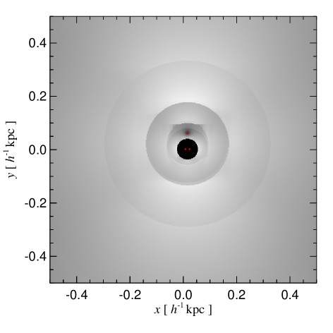
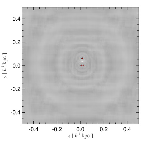
Figure 26: Maps of the relative force error in the $xy$-plane for a distribution of three points of equal mass, averaged over 100 force calculations where each time the placing of the particle configuration relative to the geometry of the underlying oct-tree is randomized. Except for this translational randomizing and averaging, the test is equivalent to that of Fig. 25. In particular, the left panel shows the result for the Tree algorithm, the right panel for the FMM method. We see that the effective force law after averaging becomes symmetric and largely eliminates discontinuities in the force accuracy (more so for FMM than for the Tree). This is achieved by reducing correlations of force errors in subsequent evaluations of the force at essentially no overhead.

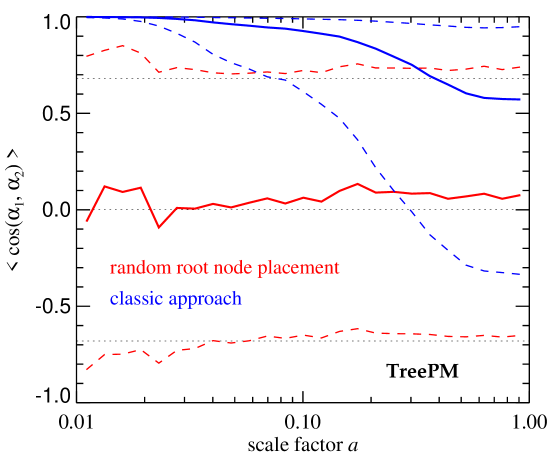
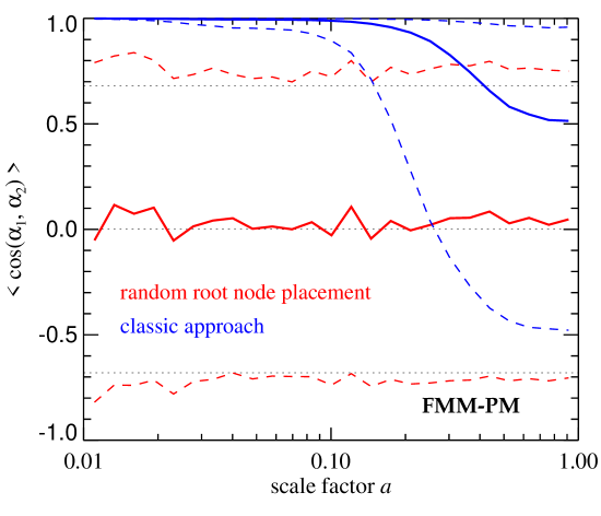
Figure 27: Temporal correlations in the direction of force errors in simulations computed with the TreePM (left panel) or FMM-PM algorithms (right panel), from high redshift to the present. The particular model examined here follows $256^{3}$ particles in a $20\,h^{-1}{\rm Mpc}$ box and is started at $z=99$. Force errors for a random set of particles are determined on the fly at times spaced $\Delta\ln a=0.009$ apart (i.e. at 512 times over the course of the simulation). We then determine the distribution of the cosine between the directions of the force errors at subsequent evaluation times, and plot the median (solid lines) and the 16% and 84% percentiles (dashed lines) as a function of scale factor. Results for the ordinary traditional simulation approach are shown in blue, while our randomization approach, where the whole particle set is randomly translated relative to the root node after each full timestep, is shown in red. Clearly, the force errors in the classical method are strongly correlated in time, whereas the randomization eliminates this successfully. Here an expansion order $p=3$ and a mesh size of $N_{\rm grid}=512$ have been used; other variants of our gravitational solvers give qualitatively very similar results.

For all algorithms discussed thus far, the residual force errors of particles are correlated in space. In the case of the Tree algorithm, this arises due to the geometric oct-tree pattern of the tree combined with the fact that neighbouring particles will have similar interaction lists, and thus experience similar errors in the specific multipole expansions they see. For the FMM algorithm, these effects can be expected to be substantially more severe, because the FFM potential expansions will generally discontinuously ‘jump’ at node boundaries, and as we have seen earlier, the errors tend to be dominated by the sink-side expansion. Similarly, we expect the grid pattern of the PM algorithm to be directly imprinted on maps of the force error distribution, and hence to introduce spatial force error correlations.

We show examples of this in Figure 25, both for the tree and the FMM algorithms. Of course, as the force errors are overall small, one may deem them to be inconsequential and disregard the fact that they are spatially correlated. A random force error without spatial and temporal correlations should indeed be largely inconsequential in collisionless dynamics, as for example Hernquist, Hut & Makino (1993) argue. But this ideal situation is not what we encounter in these standard force calculation algorithms. In particular, if a particle distribution is nearly stationary and extremely cold, as it happens in a comoving cosmological simulation at high redshift, discontinuous force errors along boundaries of large nodes, such as they occur in FMM, can easily imprint step-like artefacts in the phase-space distribution of particles that may become visible at sufficiently high mass resolution, something that we in fact did encounter when targeting simulations with extreme dynamic range in the dark matter (Wang et al., 2020), prompting us to adopt the randomization scheme described below.

Of course, one approach to mitigate such effects is to try to reduce the absolute size of the force errors as much as possible. This can be done through the use of very small opening angles, at the price of a high computational cost. Another approach is to at least eliminate the temporal correlation of the force errors. We achieve this by randomizing the relative location of the particle set with respect to the computational box by adding one random displacement vector to all particle positions each time a new domain decomposition is carried out. Note that due to our use of integer coordinates, translating the particles is a loss-less operation that is not affected by floating point round-off errors, and in particular, it is fully reversible. This randomization vector can be as large as the boxsize in each of its dimensions. This means that typically all particles move to another MPI rank in a domain decomposition, or in other words, there is a complete reshuffling of the particle data. However, already for a moderate number of MPI ranks, our domain decomposition algorithm tends to produce new solutions every timestep that have very little correlation with the previous domain decomposition anyway, so that even without randomization an effectively all-to-all exchange of the particle data in a domain decomposition could not be avoided.

The randomization may seem like a crude fix but proves actually rather effective in practice. (Recall that randomizations are also known to do wonders in other contexts, famously for example in Glimm’s 1965 method for hydrodynamics.) We demonstrate this in Figure 26, where we now show the average force error distribution after repeating it many times. We see that we now recover a purely distance-based, translationally invariant force law as desired.

The same phenomenon is also present in typical N-body simulations. In Figure 27 we show the correlations between subsequent force evolutions that are $\Delta\ln a=0.009$ apart, as a function of cosmological scale factor in a $256^{3}$ dark matter only simulation evolved from $z=99$ to $z=0$. We measure the expectation value of the cosine of the angle between the force error vector occurring for a particle at time $a$ and $a+\Delta a$. We try a TreePM and FMM-PM setup simulated with $\alpha=0.0025$, expansion order $p=3$, and a grid size $N_{\rm grid}^{3}=512^{3}$, and for each of these two setups, we run a variant in which the particle set is randomly translated with respect to the box for each timestep, and compare it to the classic treatment where no such randomization is done.

Interestingly, the TreePM and FMM-PM schemes show strong correlations of the force errors in time, as expected based on the above discussion. The correlations become weaker at low redshifts once more particles live on shorter dynamical times in halos, but even at $z=0$ remain very significant. This invokes the danger that force errors build up over time for certain particles, reducing the accuracy of their orbit integration. However, the randomization approach basically eliminates the correlation of the force errors between subsequent timesteps. In this case, the distribution function of the cosine between subsequent force error vectors is very close to uniform at any given time, meaning that while individual particles still experience force errors of the same magnitude as before, the errors tend to point into different directions for every timestep, consistent with basic requirements of collisionless dynamics (Hernquist, Hut & Makino, 1993).

4 Time integration of collisionless particles

Similar to GADGET-2, we use a kick-drift-kick formulation of a simple leapfrog integrator to advance particle orbits in time. This arises from the Hamiltonian of the particle system by considering its kinetic and potential parts alternatingly to obtain the time evolution through operator splitting. Because the two separate evolutions corresponding to the kick and drift operations are exact solutions of partial Hamiltonians, some beneficial properties of symplectic integration result, such as preservation of phase-space density, and the prevention of the build-up of long-term secular integration errors in the energy, at least as long as the timestep size stays fixed (Saha & Tremaine, 1992; Hairer, Lubich & Wanner, 2003; Hernandez & Bertschinger, 2018).

The symplectic second-order accurate leapfrog integration can be generalized to the cosmological case by introducing a conjugate momentum equal to ${\bf p}=a^{2}{\bf\dot{x}}$ for every particle as its velocity variable, where ${\bf\dot{x}}={\rm d}{\bf x}/{\rm d}t$ is the comoving velocity (Quinn et al., 1997). In the cosmological case it is advantageous to discretize time in terms of the time variable $\tau=\ln a$, because a constant $\Delta\tau$ in this case corresponds to steps that are a fixed fraction of the current Hubble time, which in turn closely tracks the dynamical time at mean density. The kick operation for a timestep $\Delta\tau$ is then given by

$${\bf p}(\tau_{n}+\Delta\tau)={\bf p}(\tau_{n})+{\bf a}_{n}(\tau_{n})\,\int_{\tau_{n}}^{\tau_{n}+\Delta\tau}\frac{{\rm d}\tau}{a\,H(a)},$$ (40)

where ${\bf a}_{n}(\tau_{n})$ is the comoving acceleration experienced by the particle at time $\tau_{n}$ (and this acceleration does not change during the time interval because the comoving positions are held fixed). Similarly, the drift operation becomes a displacement in comoving space with constant conjugate momentum, given by

$${\bf x}(\tau_{n}+\Delta\tau)={\bf x}(\tau_{n})+{\bf p}_{n}(\tau_{n})\,\int_{\tau_{n}}^{\tau_{n}+\Delta\tau}\frac{{\rm d}\tau}{a^{2}H(a)}.$$ (41)

The integrations over the Hubble rate $H(a)$ can be carried out to machine precision with a high-accuracy numerical integrator for an arbitrary Friedmann cosmology. Because the resulting timestep factors can be reused for many particles when a synchronized timestep hierarchy is used, the cost associated with these integrations is negligible.

A single timestep is then carried out as a sequence of a half-step kick, followed by a full-step drift, and a further half-step kick, i.e. the time evolution operator $E$ of one step is

$$E(\Delta t)=K\left(\frac{\Delta t}{2}\right)\circ D(\Delta t)\circ K\left(\frac{\Delta t}{2}\right),$$ (42)

yielding a second-order accurate time integration scheme. Note that only one force calculation per timestep is required, as the force calculation at the end of a timestep can be reused for the first kick operation of the subsequent step. The kick operations of two subsequent time-steps can in principle be combined into one kick, an approach followed in GADGET-2. However, in GADGET-4 we refrain from doing this merge, thereby allowing outputs to be created in between two half-step kicks, thus retaining the formal second-order accuracy in the output velocities. Also, this allows a cleaner nesting of the hydrodynamical evaluation inside the gravity steps based on operator-split principles, and it simplifies the treatment of timestep changes in the local time integration schemes we discuss next.

4.1 Traditional nested time integration

The high dynamic range in density and spatial scales that occurs in astrophysical systems is complemented by equally large variations in timescales. For example, the gravitational dynamical timescales in the centres of dark matter halos are about a factor $\sim 1000$ smaller than at the edge of halos, which are in turn nearly a factor 10 shorter than at mean density. Integrating the whole system on the shortest dynamical timescale is highly inefficient in this case. In fact, for hydrodynamical cosmological simulations, the corresponding spread in timescales can become much larger still, making it imperative that adaptive time integration schemes are used that take the local needs of each particle into account.

A popular approach to implement local time integration is to subdivide the simulation timespan into a power-of-two hierarchy, and then to require that permissable timesteps are nested within this hierarchy. This means that all timesteps are power of two multiples of the smallest occurring timestep. Particles with the same timestep size occupy a certain timestep bin in this scheme, and may change to shorter or longer timesteps when they have completed their current timestep. To maximize the amount of synchronization between different particles, one allows an increase of the timestep size only when the new target timebin is synchronized with the current time, whereas reductions of the timestep size can happen at the end of every timestep.

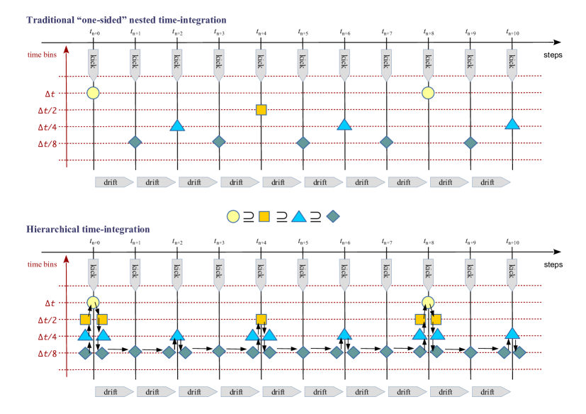
Figure 28: Sketch of the nested local time integration scheme with four occupied timebins. The top panel illustrates the “one-sided” approach where all active particles receive a force calculation from all other particles. At different synchronization times $t_{n}$ (which are spaced apart by the smallest timestep occurring in the system, here $\Delta t/8$), different sets of particles are active and require a force calculation, namely exactly those particles whose timesteps begin or end at the current synchronization time. For example, the orange squares symbolize particles with timestep $\Delta t/2$ or lower; this group includes the particles with timestep $\Delta t/4$ or lower, which in turn are represented with a blue triangle in the sketch. In between subsequent (partial) force calculations, the particle coordinates are pushed with constant momenta by cheap drift operations. The lower panel sketches the hierarchical time integration algorithm instead. At each synchronization point, it may here be necessary to compute several partial forces to carry out the correct kick operation. Each partial force only involves force calculations where source and sink sets are equal, i.e. here the occurrence of a symbol in the sketch means that a force calculation of the corresponding subset of particles with itself as source (as opposed to the whole particle distribution) is required. All momentum changes in this scheme are based on pair-wise forces that manifestly preserve total momentum.

A sketch of the resulting integration scheme for an example with four active timebins is shown in the top panel of Figure 28. We call this scheme of local time integration “one-sided”, because every active particle receives a force from the full particle distribution (which therefore also needs to be drifted to the current time). Momentum conservation is here not manifest between all pairs of interacting particles, even in the absence of any force errors. One may nevertheless hope that no significant momentum error builds up in practice due to this, because time averaging should largely eliminate the build-up of sizeable momentum errors from one-sided interactions in the limit of small timesteps.

4.2 Hierarchical time integration

Two issues remain unsatisfactory with the above. First, active particles couple asymmetrically with the whole system, spoiling manifest momentum conservation. Secondly, the computational cost does not go down linearly with the fraction of active particles, because to construct the tree, one still needs to synchronize (i.e. drift) all particles and make them part of the tree in the first place. This behaviour can be improved by a systematic, hierarchical decomposition of the Hamiltonian dynamics, which we implement similarly as described in Pelupessy, Jänes & Portegies Zwart (2012), and used already successfully within the AREPO code in production for the IllustrisTNG simulations (Marinacci et al., 2018; Nelson et al., 2018; Naiman et al., 2018; Pillepich et al., 2018; Springel et al., 2018), as well as for the ‘Void-in-Voids-in-Voids’ simulations of Wang et al. (2020). Recently, another implementation of this approach has been described by Zhu (2020), who also combined this with FMM for the first time.

First, it is perhaps useful to recall second-order operator split methods to integrate a Hamiltonian system of the form

$$H=H_{1}+H_{2},$$ (43)

which can for example be done through

$$E(H,\Delta t)\simeq E\left(H_{1},\frac{\Delta t}{2}\right)\circ E(H_{2},{\Delta t})\circ E\left(H_{1},\frac{\Delta t}{2}\right),$$ (44)

where $E(H,\tau)$ is the time evolution operator of the system under a Hamiltonian $H$ over time $\tau$. This is what we already used to construct our basic leapfrog scheme, which for fixed timesteps is symplectic. The schemes constructed below are also symplectic because they still arise as exact solutions of partial Hamiltonians that are alternatingly applied to advance the system. Their symplectic nature is however lost once particles change their timesteps, just like it happens in the ordinary leapfrog.

Consider now a particle system P described by the Hamiltonian:

$$H=H_{\rm kin}+H_{\rm pot}.$$ (45)

Suppose we are given a timestep $\Delta t$. Then we can subdivide the particle system into a “slow” and a “fast” part, ${\rm P=S+F}$, based on the notion that the slow system S contains the particles for which an integration with the given timestep size would be sufficiently accurate, while the fast system F gets the particles where the integration timestep should be chosen smaller. After the subdivision, we can write the Hamiltonian as

$$H=H_{\rm kin}^{\rm S}+H_{\rm pot}^{\rm S}+H_{\rm kin}^{\rm F}+H_{\rm pot}^{\rm F}+H_{\rm pot}^{\rm FS},$$ (46)

or equivalently

$$H=H^{\rm S}+H^{\rm F}+H_{\rm pot}^{\rm FS},$$ (47)

where now $H^{\rm S}=H_{\rm kin}^{\rm S}+H_{\rm pot}^{\rm S}$ and $H^{\rm F}=H_{\rm kin}^{\rm F}+H_{\rm pot}^{\rm F}$ are Hamiltonians that only involve the slow and fast particles, respectively. The interaction term $H_{\rm pot}^{\rm FS}$ accounts for all potential terms that involve mixed particle pairs.

The time evolution of the system could now for example be approximated to second-order in $\Delta t$ as:

$$E(H,\Delta t) \simeq E\left(H_{\rm pot}^{\rm FS},\frac{\Delta t}{2}\right)\circ E\left(H^{\rm F},\frac{\Delta t}{2}\right)\circ E(H^{\rm S},{\Delta t})\circ$$ (48)

$$E\left(H^{\rm F},\frac{\Delta t}{2}\right)\circ E\left(H_{\rm pot}^{\rm FS},\frac{\Delta t}{2}\right).$$

Here the slow system is evolved on a timestep $\Delta t$, which by construction was deemed sufficient to integrate the corresponding particles. This step can hence be replaced with, e.g., a single leap-frog step of size $\Delta t$. In contrast, the fast part is evolved on half the timestep by the corresponding operators, and a single timestep may not necessarily be sufficient for doing this accurately. But in this case, we can reduce the timestep for this part by subcycling (see below). For the interaction component, we shall assume that the timestep of $\Delta t/2$ is sufficient to do it in a single step with sufficient accuracy, on the grounds that all terms involve one of the slow particles.

We now specialize to an N-body system and employ the kick- and drift operators for evolution under the kinetic and potential terms, respectively. Then the time evolution described by equation (48) can be written as:

$$E(H,\Delta t) \simeq K_{\rm S}^{\rm F}\left(\frac{\Delta t}{2}\right)K_{\rm F}^{\rm S}\left(\frac{\Delta t}{2}\right)$$ (49)

$$E\left(H_{\rm F},\frac{\Delta t}{2}\right)$$

$$K_{\rm S}^{\rm S}\left(\frac{\Delta t}{2}\right)D_{\rm S}\left({\Delta t}\right)K_{\rm S}^{\rm S}\left(\frac{\Delta t}{2}\right)$$

$$E\left(H_{\rm F},\frac{\Delta t}{2}\right)$$

$$K_{\rm S}^{\rm F}\left(\frac{\Delta t}{2}\right)K_{\rm F}^{\rm S}\left(\frac{\Delta t}{2}\right).$$

In this notation, the kick operator $K_{\rm A}^{\rm B}$ means that forces due to particles in set B are applied to the particles in A. Note that $K_{\rm S}^{\rm S}$ commutes with the time evolution operator for the fast part of the Hamiltonian, $H^{\rm F}$, simply because they operate on disjoint particle sets. We are hence free to move the first occurrence of $K_{\rm S}^{\rm S}$ in front of the first $E(H_{F})$ operator, and the second $K_{\rm S}^{\rm S}$ behind the second $E(H_{F})$. The individual kick operators also commute, and $D_{\rm S}$ could as well be interchanged with operators that only involve the fast particles. We are thus free to alternatively express equation (49) as

$$E(H,\Delta t) \simeq K_{\rm P}^{\rm P}\left(\frac{\Delta t}{2}\right)K_{\rm F}^{\rm F}\left(-\frac{\Delta t}{2}\right)$$ (50)

$$E\left(H_{\rm F},\frac{\Delta t}{2}\right)D_{\rm S}\left({\Delta t}\right)E\left(H_{\rm F},\frac{\Delta t}{2}\right)$$

$$K_{\rm F}^{\rm F}\left(-\frac{\Delta t}{2}\right)K_{\rm P}^{\rm P}\left(\frac{\Delta t}{2}\right),$$

where we used $K_{\rm S}^{\rm F}({\Delta t})K_{\rm F}^{\rm S}({\Delta t})K_{\rm S}^{\rm S}({\Delta t})=K_{\rm P}^{\rm P}({\Delta t})K_{\rm F}^{\rm F}(-{\Delta t})$.

This is now essentially in the form we recursively apply it in practice. We first start out by calculating the forces for the whole system P. This in particular allows us to apply the $K_{\rm P}^{\rm P}$ operator. Also, we can then use the size of the forces calculated for P to distinguish between the F and S particles by means of a timestep criterion. For the particles ending up in F, new forces are then calculated, sourced just by those in the set F, allowing us to partially undo the previous kick, through the $K_{\rm F}^{\rm F}$ operator. These F particles are then treated as a new system P’, for which we now need to carry out the time evolution over a timestep $\Delta t/2$. This can be dealt with recursively by applying the same procedure yet again, with P’ becoming the new P. In doing this, the first task, namely the calculation of all forces for $P^{\prime}$ has already just been done previously (as force calculation for the set F), and thus the corresponding force calculations can be recycled. Also note that the forces entering the timestep criterion for deciding between fast and slow particles in deeper levels of the hierarchy become partial forces originating in ever smaller subsets P’ of the system. The recursive subdivision into ever smaller particle sets ends once the set F becomes empty. At this point, a drift for the current set F is carried out, followed by a force calculation for this set and a closing half-step kick. Then a drift of the slow system is done (which may however also be delayed to a later time, just before the next force calculation that involves any of the slow particles), followed again by a kick-drift-kick sequence of the fast part. Finally, one closes off the step by partially undoing the kick of the fast system (with already known forces at this point), followed by a force calculation for P at the end of the step, and a full kick of the full system. The recursive application of the scheme means that depending on where the closing step occurs one may have to back out of multiple levels of subdivisions, since all the levels are nested into each other in a power-of-two timestep hierarchy. The lower panel of Figure 28 shows a sketch of this scheme for an example involving four active timebins.

One important feature of this time integration method is that the fast system that is split off is self-contained, i.e. its evolution does not rely on any residual coupling with the slow particles. In particular, one does not have to construct the tree for all particles when the forces on F are required; only the particles from F are needed. Another aspect is that all the forces that are applied are for operators of the form $K_{\rm A}^{\rm A}$ only, where source and sink sets are equal. This implies manifest momentum conservation for the local time integration scheme, something that is not the case in the traditional method to implement local timesteps where ‘one-sided’ forces between particle pairs occur. Furthermore, when a fast multipole moment method is applied to compute the gravitational forces, the momentum conservation will be manifest to machine precision despite the presence of finite force approximation errors.

However, this advantage comes at the price of additional force computations relative to the ordinary “one-sided” nested time integration. To quantify this, let us index the highest occupied timebin with $k=0$, and call $N_{k}$ the number of particles with timestep $\Delta t=\Delta t_{\rm max}/2^{k}$ or lower, where $\Delta t_{\rm max}$ is the maximum occupied timestep. Note that $N_{0}$ is thus the total particle number.

For the ordinary nested time integration, at any given synchronization point of the timestep hierarchy only one force calculation is necessary. To advance the whole system over $\Delta t_{\rm max}$, a number of

$$K_{\rm onesided}=N_{0}+\sum_{k=1}^{k_{\rm max}}2^{k-1}\,N_{k}$$ (51)

force computations is necessary. If the simulated timespan is $T_{\rm sim}$, the total number of force computations for the simulation is then $T_{\rm sim}/\Delta t_{\rm max}\times K_{{\rm onesided}}$. In contrast, for the hierarchical time integration scheme, the cost is characterized by

$$K_{\rm hierarchical}=N_{0}+3\times\sum_{k=1}^{k_{\rm max}}2^{k-1}\,N_{k}$$ (52)

force computations. At face value this can be substantially larger than the one-sided scheme, in the worst case by something that approaches a factor of 3.

However, there are several reasons that mitigate this difference in practice, and can make the hierarchical integration nevertheless worthwhile. First of all, in many cases the hierarchical integration can deliver improved accuracy at equal timestep size, meaning that some of the extra cost can be absorbed into a somewhat larger timestep. Depending on the timestep criterion and simulation set-up, there can also be situations where the hierarchical timestep criterion leads to a less deep timestep hierarchy (for example when large-scale accelerations are caused by particles on long timesteps, which then do not enter any more in relative motions on small-scales), making the hierarchical integration more efficient by altering the occupancy $N_{k}$ on the different timestep bins.

Leaving this aside, we also see that for the hierarchical integration it can make sense to restrict the maximum allowed timestep to something smaller than $\Delta t_{\rm max}$. This happens when we would otherwise have $N_{1}>N_{0}/3$, i.e. whenever the first time bin below the maximum timestep holds more than one third of the particles. In this case, it is actually beneficial to rather use a shorter maximum timestep $\Delta t_{\rm max}/2$ for all particles, as this reduces the cost sum $K_{\rm hierarchical}$ while at the same time it increases the time integration accuracy. The code automatically detects this condition and modifies the timesteps of the particles accordingly.

Importantly, whether or not the cost increase of hierarchical integration is substantial depends sensitively on the depth of the timestep hierarchy, and how the occupancy $N_{k}$ varies with the timebin $k$. If we always have $N_{k+1}<N_{k}/2$ (which is common in cosmological simulations, in fact, quite typically the occupancy declines more steeply than this), then the total cost is dominated by timebins with the longest timesteps, despite the short timesteps being executed (much) more frequently. If we additionally have $N_{1}\ll N_{0}/3$, then there is no significant cost difference between hierarchical and ordinary time integration left when measured in terms of the number of force calculations.

However, as noted earlier, there is an important further difference between the two approaches. For the one-sided time integration, the force computations require a tree construction for the full particle set, as well as drifting these particles to the current synchronization point. In contrast, for the hierarchical integration scheme, the tree has to be constructed only for the particle set involved in the current force computation. If the timebin hierarchy is very deep, the one-sided scheme can then become dominated by the (constant) tree construction costs, whereas this cost declines for the hierarchical integration alongside the smaller occupancy at ever deeper timebin levels. For very deep timestep hierarchies, it is therefore the hierarchical integration that can outperform the ordinary time integration, because it can avoid becoming dominated by tree construction overhead and particle drift costs. The hierarchical approach has therefore better potential for simulations with an extreme dynamic range in timescales.

4.3 Timestepping for TreePM and FMM-PM

A problem shared by the Tree-PM and FMM-PM approaches when local time integration is used is that the PM part of the algorithm does not require significantly reduced computational time if forces for only a subset of the particles need to be calculated. To avoid an inefficiency of TreePM/FMM-PM for local time integration, GADGET-2 introduced a scheme (which is optionally still supported in GADGET-4) where the TreePM force-split also induces a split in the associated time integration, based again on the concept of operator splitting. When one PM mesh covers the whole simulation domain, the gravitational part of the Hamiltonian can be split into a long-range and a short-range part,

$$H_{\rm pot}=H_{\rm long}^{\rm PM}+H_{\rm short}^{\rm{tree}}$$ (53)

with a single split scale, allowing us to write the evolution of the system over one timestep $\Delta t$ as

$$E(H,\Delta t)=K_{\rm long}^{\rm PM}\left(\frac{\Delta t}{2}\right)\circ E(H_{\rm short},\Delta t)\circ K_{\rm long}^{\rm PM}\left(\frac{\Delta t}{2}\right),$$ (54)

where $K_{\rm long}^{\rm PM}$ refers to kicks due to the long-range PM force, and $H_{\rm short}=H_{\rm kin}+H_{\rm short}^{\rm{tree}}$ describes the short-range dynamics, which now can be treated either with the hierarchical scheme as introduced above, or with the one-sided nested time-stepping approach. The timestep $\Delta t_{\rm PM}$ chosen as appropriate for the long-range PM forces is then also equal to the maximum timestep in the system.

If a secondary high-resolution PM mesh is used following the approach outlined earlier, the potential energy can still be subdivided into two terms, but the split-scale applied to each particle pair now depends on their spatial coordinates. The associated time-scales on which the long range forces change can then also differ significantly between the high-resolution and the background regions, which may require considerably more conservative settings for $\Delta t_{\rm PM}$.

Another approach to avoid the PM overhead in thinly populated timebins is to decide on-the-fly for every force calculation whether it should be carried out through the Tree-PM/FMM-PM approach, or through a pure Tree/FMM with Ewald correction when periodic boundaries are used. This time-integration option is newly supported in GADGET-4, and we refer to it as the ‘time-unsplit Tree-PM/FMM-PM scheme’, because here the PM algorithm is used to speed up force computations without influencing the time integration. Because of this property, we in principle prefer this approach on conceptual grounds. In practice, we define a run-time parameter that controls the hand-over point between force computations carried out with Tree-PM/FMM-PM, or with a pure Tree/FMM instead. If the fraction of active particles is larger than a specified value, the PM approach is used to accelerate the force calculations, otherwise the pure multipole algorithms are applied. In this way, one can benefit from the higher speed of the PM-based approach for reasonably full timesteps, while thinly populated timebins can be dealt with without the overhead of doing large FFTs for only a small number of particles.

4.4 Summary of time-integration and force computation schemes

GADGET-4 supports a perhaps bewildering variety of different combinations of force computation and time integration schemes. For definiteness, let us illustrate this with the common case of a cosmological simulation with periodic boundary conditions integrated in comoving coordinates. Such a simulation can in principle be carried out either with a pure Tree with Ewald corrections, a Tree-PM scheme with an induced split in the timesteps of long-range and short-range forces, or with a Tree-PM scheme without such a split. Each of these three possibilities can be either combined with a classic one-sided local timestepping scheme, or with the new hierarchical time integration method introduced in this paper. This yields 6 different basic combinations. Furthermore, for each of these 6 combinations the Tree part of the calculations can be replaced with the FMM method, doubling this to already 12 different variations, as schematically summarized in Table 2. Finally, one can run each of these cases with different multipole oder $p$. If one considers each of these choices as different force calculation algorithms, one arrives at 60 possible ways to do the calculation. In zoom-simulations, the possibility to use an additional secondary Fourier mesh covering the high-resolution region adds even further possibilities.

All of these approaches should give the same results when carried out with conservative settings for time integration and force accuracy. It is an important validation test to explicitly verify that this is actually the case, something we have tried to ensure during the tests of the code. However, it is of course expected that the different methods may differ quite drastically in the required CPU-time for a prescribed accuracy level. Especially for cosmological simulations of structure formation, the pure Tree and FMM algorithms at low order $p$ should be slowest, both due to the high force accuracy demands at high-$z$, which are costly to reach with a low-order multipole expansion algorithm, and the need to Ewald-correct all the force contributions.

The PM-accelerated versions and the use of higher order $p$ are expected to do a lot better in terms of CPU cost, but where the optimum lies is unfortunately problem-dependent. Similarly, whether or not the use of hierarchical timestepping is an advantage in terms of performance depends critically on the depth of the timestep hierarchy. If the latter is very deep, it can yield a performance advantage, because the code can save on tree construction time, and also does not need to synchronize passive particles. If it is shallow, these advantages will be overwhelmed by the additional force calculations and tree constructions that are necessary in the hierarchical scheme. In most scenarios, we expect the FMM approach to be faster than the one-sided Tree, at least for global timesteps, with its main downside being the somewhat higher memory need, the somewhat less ideal parallel scalability, and the poor performance of FMM for thinly populated timebins in local one-sided time integration schemes, so that one is more or less forced to use hierarchical time integration for FMM. Note that in our implementation FMM needs to compute interactions between nodes that are stored on two different processors on both processors, i.e. twice, so that the associated overhead slowly grows for fixed problem size with the number of employed distributed-memory compute nodes.

To what extent all of these general expectations are borne out in practice with the current implementation of GADGET-4 can only be decided through explicit tests of the performance for scientifically relevant setups. We report the results of a set of tests along these lines in Section 10, providing some guidance for the selection of the most efficient algorithm for a particular problem. But we stress that we want to refrain from general advice about which set-up is best, as such statements can easily be misleading due to the complicated dependence of performance on the problem type and the desired accuracy, and because details of the technical computing environment such as the type of processor and the speed of the communication backplane play a role as well.

	pure tree	with mesh acceleration
	with Ewald	no Ewald	sometimes Ewald
Tree-Based	Tree	TreePM	TreePM-NoS
	H-Tree	H-TreePM	H-TreePM-NoS
FMM-Based	FMM	FMM-PM	FMM-PM-NoS
	H-FMM	H-FMM-PM	H-FMM-PM-NoS

Table 2: Different combinations of gravitational force calculation and time integration schemes supported in GADGET-4. Variations with a prefix ‘H-’ refer to use of the hierarchical time integration scheme. Tree and FMM designate that the hierarchical multipole calculation is done either with a classic one-sided Barnes & Hut tree code, or with a fast multipole method. We note that each of these combinations can be run with different multipole order, $p=1$ to $p=5$. For the PM schemes, Fourier methods are used to accelerate the calculation of long-range forces. In the plain TreePM and FMM-PM approaches this is also inducing a split of the time integration into long- and short range dynamics. In the NoS variants of these schemes, no such split in the time integration is done, instead the forces are either computed with a pure multipole method, or with a PM acceleration, depending on the active particle fraction. Note that in zoom simulations, the PM variants of the algorithms can optionally be combined with the placement of additional Fourier mesh on the high-resolution region.

5 Hydrodynamical discretization

A versatile and conceptually simple approach for simulating hydrodynamics is the smoothed particle hydrodynamics (SPH) technique (Gingold & Monaghan, 1977; Monaghan, 1992). It has a long history in astrophysics, where some of its main advantages, such as automatic spatial adaptivity, robustness, ability to deal with nearly empty space, and ease of coupling to collisionless dynamics used for dark matter and stars are particularly attractive points (see Springel, 2010b; Price, 2012; Rosswog, 2015, for reviews).

However, over the past decade, accuracy problems of SPH in certain regimes have been pointed out and seen intense scrutiny (Agertz et al., 2007; Bauer & Springel, 2012). In certain regimes, standard formulations of SPH have been found to be very noisy or suppress fluid instabilities, causing concerns about the general applicability of this technique. In turn, this triggered intense efforts to improve or resolve these problems. Proposed solutions range from relatively small refinements such as better artificial viscosity prescriptions or the use of different smoothing kernels, over different formulations of the equations of motion, to more radical changes of the underlying discretization principle (e.g. Ritchie & Thomas, 2001; Price, 2008; Heß & Springel, 2010; Gaburov & Nitadori, 2011; Murante et al., 2011; McNally, Maron & Mac Low, 2012; Valdarnini, 2012; Read & Hayfield, 2012; Hopkins, 2013, 2015; Beck et al., 2016; Frontiere, Raskin & Owen, 2017). Also new types of quasi-Lagrangian discretizations that are mesh rather than particle-based, such as the moving-mesh code AREPO (Springel, 2010a), have been proposed.

However, SPH remains useful as a low-order technique because it often gives surprisingly robust and qualitatively correct results, even when the particle number per object is small (Schaller et al., 2015; Huang et al., 2019), although there are also regimes where important systematic effects due to its numerical inaccuracies show up in galaxy formation simulations (e.g. Sijacki et al., 2012; Nelson et al., 2013). We have thus improved the original implementation of SPH in GADGET-2. The implementation included in GADGET-4 offers enhanced performance and features a few of the proposals made for a more ‘modern’ flavour of SPH. Which of the many improvements suggested in recent years for SPH will ultimately prevail is however still an unsettled issue, as illustrated by diversity of approaches in the recent SPH literature. Contributing to this debate is beyond the scope of this work, hence we restrict ourselves to contribute a modernized code base that allows SPH simulations to be pushed to large sizes and which should be a useful platform to easily make further improvements to the basic formulation.

In GADGET-4, we presently support both ‘vanilla SPH’, as originally defined in terms of the conservative entropy formulation (Springel & Hernquist, 2002) of standard SPH (Monaghan & Gingold, 1983), as well as the ‘pressure-based’ variant P-SPH (Hopkins, 2013), which behaves better at contact discontinuities. Besides these two basic formulations of the equations of motion, also the role of the kernel has been emphasized in the recent SPH literature. In particular, the Wendland (1995) kernels suggested by Dehnen & Aly (2012) provide protection against the so-called clumping instability, and thus allow a larger neighbours number to mitigate the inherent noise in SPH. We offer both the traditional cubic spline kernel, and the Wendland kernels at order 2, 4, and 6. We note however that the Wendland kernels require substantially larger number of neighbours for a given resolution, and it is problem dependent whether their use is advantageous (see also Zhu, Hernquist & Li, 2015).

Finally, a third area where substantial improvements have been made concerns the use of sophisticated parameterizations of artificial viscosity. Here we include only one of the simpler recent suggestions. We do not include an implementation of explicit mixing terms between SPH particles (Price, 2008), such as artificial heat conduction, which has been shown to be beneficial for certain problems. This can however be easily added to the code base if desired.

5.1 Basic SPH formulation

5.1.1 Standard (‘vanilla’) SPH

As discussed by Springel & Hernquist (2002), the inviscid part of the hydrodynamics of an ideal gas discretized with SPH can be generated by an interaction Hamiltonian of the form

$$H_{\rm therm}=\sum_{i}m_{i}A_{i}\frac{\rho_{i}^{\gamma-1}}{\gamma-1},$$ (55)

where $A_{i}$ denotes the entropic function of particle $i$, and $\rho_{i}$ is its density. The pressure is given by the ideal gas law $P_{i}=A_{i}\rho_{i}^{\gamma}$ with adiabatic index $\gamma$. The densities are estimated with adaptive kernel estimation,

$$\rho_{i}=\sum_{j}m_{j}W({\bf r}_{ij},h_{i}),$$ (56)

where $W({\bf r},h)$ is a spherically symmetric smoothing kernel, and the smoothing lengths $h_{i}$ are determined through the implicit constraint $\rho_{i}h_{i}^{3}/m_{i}=const.$

The Euler-Lagrange equations of motion then create antisymmetric pair-wise pressure forces

$$\frac{{\rm d}{\bf v}_{i}}{{\rm d}t}=-\sum_{j=1}^{N}m_{j}\left[f_{i}\frac{P_{i}}{\rho_{i}^{2}}\nabla_{i}W_{ij}(h_{i})+f_{j}\frac{P_{j}}{\rho_{j}^{2}}\nabla_{i}W_{ij}(h_{j})\right],$$ (57)

where the $f_{i}$ are defined by

$$f_{i}=\left[1+\frac{h_{i}}{3\rho_{i}}\frac{\partial\rho_{i}}{\partial h_{i}}\right]^{-1},$$ (58)

and the abbreviation $W_{ij}(h)=W(|{\bf r}_{i}-{\bf r}_{j}|,h)$ has been used.

5.1.2 Pressure based formulation

The above formulation conserves both energy and entropy, but shows a spurious surface tension at phase boundaries. This tends to suppress or slow the growth of fluid instabilities at contact discontinuities. The ‘pressure-based’ variational formulation of Hopkins (2013) can significantly improve on this, at the price of a somewhat higher noise in other parts of the flow. Instead of estimating the density, the pressure is estimated by

$$P_{i}=\left[\sum_{j}m_{j}A_{j}^{1/\gamma}W({\bf r}_{ij},h_{i})\right]^{\gamma}.$$ (59)

The equation of motion is given by

$$\frac{{\rm d}{\bf v}_{i}}{{\rm d}t}=-\sum_{j=1}^{N}m_{j}\left(A_{i}A_{j}\right)^{1/\gamma}\left[f_{ij}\frac{P_{i}}{P_{i}^{2/\gamma}}\nabla_{i}W_{ij}(h_{i})+f_{ji}\frac{P_{j}}{P_{j}^{2/\gamma}}\nabla_{j}W_{ij}(h_{j})\right],$$ (60)

with the correction term

$$f_{ij}=1-\left(\frac{h_{i}}{3A_{j}^{1/\gamma}\rho_{i}}\frac{\partial P_{i}^{1/\gamma}}{\partial h_{i}}\right)\left[1+\frac{h_{i}}{3\rho_{i}}\frac{\partial\rho_{i}}{\partial h_{i}}\right]^{-1}$$ (61)

for variable smoothing lengths. As in our density formulation of SPH we determine the smoothing length by the condition $h_{i}^{3}\rho_{i}/m_{i}=const.$, which is equivalent to the condition of a fixed amount of particles in the kernel if the mass of all particles is the same.

Although for the equations of motion no estimate of the density is needed, other modules of GADGET-4, e.g. the artificial viscosity or radiative cooling, might still depend on it. We additionally calculate the density according to equation (56) for these purposes, rather than estimating it through $\rho_{i}=\left(P_{i}/A_{i}\right)^{1/\gamma}$ from the smoothed pressure.

5.2 Kernel functions

Much of the SPH-based literature of the last decades has been using the $M_{4}$ cubic spline kernel from the B-spline family. When using it, we set in $\nu$ dimensions $W(r,h)=h^{-\nu}w_{\rm M4}\left(\frac{r}{h}\right)$, with

$$w_{\rm M4}(q)=\frac{8}{\pi}\left\{\begin{array}[]{ll}1-6q^{2}+6q^{3},&0\leq q\leq\frac{1}{2},\\ 2\left(1-q\right)^{3},&\frac{1}{2}<q\leq 1,\\ 0,&q>1,\end{array}\right.$$ (62)

in three-dimensional normalization. Note that in the convention we use here, the kernel drops to zero at a distance of $r=h$, i.e. the smoothing length $h$ is equal to the finite support of the kernel (parts of the SPH literature instead define $h$ such that the kernel drops to zero at $2h$).

Occasionally, higher order kernels like quartic or quintic kernels from the same family have been used as well. Much of the recent discussion about kernel choices has however been started by Dehnen & Aly (2012) who pointed out that the three-dimensional Wendland (1995) kernels protect against the clumping instability, thus allowing the larger neighbour numbers required for reducing the kernel-interpolation errors. This comes however at the price of a significantly larger base neighbour number needed to reduce the inherent bias of the Wendland kernels to acceptable levels, making these kernels fairly expensive. We include the $C_{2}$ Wendland kernel, given by

$$w_{\rm C2}(q)=\frac{21}{\pi}\left\{\begin{array}[]{ll}(1-q)^{4}(4q+1),&0\leq q\leq 1,\\ 0,&q>1,\end{array}\right.$$ (63)

the $C_{4}$ kernel defined by

$$w_{\rm C4}(q)=\frac{495}{32\pi}\left\{\begin{array}[]{ll}(1-q)^{6}\left(\frac{35}{3}q^{2}+6q+1\right),&0\leq q\leq 1,\\ 0,&q>1,\end{array}\right.$$ (64)

and the $C_{6}$ kernel given by

$$w_{\rm C6}(q)=\frac{1365}{64\pi}\left\{\begin{array}[]{ll}(1-q)^{8}(32q^{3}+25q^{2}+8q+1),&0\leq q\leq 1,\\ 0,&q>1,\end{array}\right.$$ (65)

as alternatives to our standard kernel choice. For these kernels, from $92$ (for $C_{2}$) up to $356$ (for $C_{6}$) neighbouring particles are recommended, respectively. We note that one small technical advantage of the Wendland kernels is that they are not defined in a piecewise fashion. This makes it slightly easier to apply vector instructions for an on-the-fly evaluation of the kernel because if-conditions that branch on the value of $r$ are not needed. For completeness we also implemented the one-dimensional and two-dimensional forms of all kernel functions defined above following Dehnen & Aly (2012).

5.3 Artificial viscosity

To provide irreversible dissipation of kinetic energy into heat at shock fronts, an artificial viscosity needs to be added to the ideal gas discretization introduced above. A difficulty is to find a parameterization that is both sensitive to the presence of even weak shocks, but at the same time does not apply viscous forces outside of shocks, which would make the scheme unnecessarily diffusive (Cullen & Dehnen, 2010; Read & Hayfield, 2012; Hosono, Saitoh & Makino, 2016).

We add the viscous force to the equation of motion as

$$\left.\frac{{\rm d}{\bf v}_{i}}{{\rm d}t}\right|_{\rm visc}=-\sum_{j=1}^{N}m_{j}\Pi_{ij}\nabla_{i}\overline{W}_{ij}\,,$$ (66)

where

$$\overline{W}_{ij}=\frac{1}{2}\left[W_{ij}(h_{i})+W_{ij}(h_{j})\right]$$ (67)

denotes a symmetrized kernel between the two particles involved. In order to conserve total energy, we need to compensate the work done against the viscous force through generation of heat, which we do in terms of an entropy increase with a rate:

$$\left.\frac{{\rm d}A_{i}}{{\rm d}t}\right|_{\rm visc}=\frac{1}{2}\frac{\gamma-1}{\rho_{i}^{\gamma-1}}\sum_{j=1}^{N}m_{j}\Pi_{ij}{\bf v}_{ij}\cdot\nabla_{i}\overline{W}_{ij}\,,$$ (68)

where ${\bf v}_{ij}={\bf v}_{i}-{\bf v}_{j}$.

There is a lot of freedom in the detailed parameterization of the viscosity $\Pi_{ij}$. Most commonly, some variant of the form introduced by Monaghan & Gingold (1983) is employed, which is

$$\Pi_{ij}=\left\{\begin{tabular}[]{cl}${\left[-\alpha c_{ij}\mu_{ij}+\beta\mu_{ij}^{2}\right]}/{\rho_{ij}}$&\mbox{if ${\bf v}_{ij}\cdot{\bf r}_{ij}<0$}\\ 0&\mbox{otherwise},\\ \end{tabular}\right.$$ (69)

with

$$\mu_{ij}=\frac{h_{ij}\,{\bf v}_{ij}\cdot{\bf r}_{ij}}{\left|{\bf r}_{ij}\right|^{2}+\epsilon h_{ij}^{2}},$$ (70)

and which can be viewed as a combination of a bulk and a von Neumann-Richtmyer viscosity. Here $h_{ij}$ and $\rho_{ij}$ denote arithmetic means of the corresponding quantities for the two particles $i$ and $j$, with $c_{ij}$ giving the mean sound speed, whereas ${\bf r}_{ij}\equiv{\bf r}_{i}-{\bf r}_{j}$ is the particle distance vector. The strength of the viscosity is regulated by the parameters $\alpha$ and $\beta$, with typical values in the range $\alpha\simeq 0.5-1.0$ and the frequent choice of $\beta=2\,\alpha$. The parameter $\epsilon\simeq 0.01$ is introduced to protect against singularities if two particles happen to get very close. Because the viscosity factor $\Pi_{ij}$ is symmetric in $i$ and $j$, the viscous force between any pair of interacting particles is antisymmetric and along the line joining the particles, hence linear momentum and angular momentum remain preserved. The viscosity only acts for particles that rapidly approach each other, and the entropy production associated with it is always positive definite.

As discussed for GADGET-2 (Springel, 2005), we have a slight preference for a related variant of the viscosity parameterization, as proposed by Monaghan (1997) based on an analogy to the Riemann problem. This is given by

$$\Pi_{ij}=-\frac{\alpha}{2}\frac{v_{ij}^{\rm sig}w_{ij}}{\rho_{ij}},$$ (71)

where $v_{ij}^{\rm sig}=\left[c_{i}+c_{j}-3w_{ij}\right]$ is an estimate of the signal velocity between two particles $i$ and $j$, and $w_{ij}={{\bf v}_{ij}\cdot{\bf r}_{ij}}/{\left|{\bf r}_{ij}\right|}$ is the relative velocity projected onto the separation vector. This parameterization of the viscosity is used by GADGET-4 as default.

The viscosity vanishes for solid-body rotation, but not for pure shear flows. To cure this problem in shear flows, Balsara (1995) suggested adding a heuristic correction factor to the viscosity that reduces its strength when the shear is strong. We include this by multiplying $\Pi_{ij}$ with a prefactor $(f_{i}^{\rm AV}+f_{j}^{\rm AV})/2$, where the factors

$$f_{i}^{\rm AV}=\frac{|\nabla\cdot{\bf v}|_{i}}{|\nabla\cdot{\bf v}|_{i}+|\nabla\times{\bf v}|_{i}}$$ (72)

are characterizing the rate of compression in relation to the local shear. The velocity divergence and curl are computed alongside the density estimates.

Another popular modification are time-dependent viscosity schemes that aim to ramp up the viscosity only in regions of shocks while in other regions the numerical viscosity should be reduced as much as possible (Morris & Monaghan, 1997; Dolag et al., 2005; Cullen & Dehnen, 2010). We here use a formulation proposed by Hu et al. (2014) to which we refer for full details. For every particle we define a target viscosity parameter

$$\alpha_{{\rm tar},i}(t)=\alpha_{\rm max}\frac{h_{i}^{2}S_{i}}{h_{i}^{2}S_{i}+c_{i}^{2}},$$ (73)

with a shock indicator $S_{i}=\max(0,-\dot{\nabla}\cdot{\bf v}_{i})$. The actual viscosity parameter $\alpha_{i}(t)$ applied to a particle is evolved as

$$\alpha_{i}(t+{\rm d}t)=\left\{\begin{array}[]{ll}\xi_{i}\,\alpha_{{\rm tar},i}&\alpha_{i}\leq\alpha_{{\rm tar},i},\\ \xi_{i}\left[\alpha_{{\rm tar},i}+(\alpha_{i}-\alpha_{{\rm tar},i})\exp(-{\rm d}t/\tau_{i})\right],&\alpha_{i}>\alpha_{{\rm tar},i},\end{array}\right.$$ (74)

where ${\rm d}t$ gives the time step, and $\tau_{i}=10h_{i}/v_{\rm dec}$ is a decay time with the decay velocity defined as

$$v_{{\rm dec}}=\max_{{\bf r}_{ij}\leq h_{i}}\left[c_{i}+c_{j}-\min(0,{\bf v}_{ij}\cdot{\bf r}_{ij}/r_{ij})\right].$$ (75)

$\xi_{i}$ is a limiter defined by:

$$\xi_{i}=\frac{|\nabla\cdot{\bf v}_{i}|^{2}}{|\nabla\cdot{\bf v}_{i}|^{2}+|\nabla\times{\bf v}_{i}|^{2}+0.0001(c_{i}/h_{i})^{2}}.$$ (76)

To improve the accuracy of the time-dependent viscosity we have also implemented higher order velocity gradient estimates using matrix inversions, as discussed in the appendix of Hu et al. (2014).

5.4 Cooling and star formation

One of the areas where SPH has been particular popular is the simulation of galaxy and star formation, as here the automatic adaptivity and the ease with which source functions and subgrid models can be coupled to SPH come in particularly handy. Current physics modelling in SPH has reached a high degree of complexity and diversity, as can be inferred from recent work, for example on simulating the interstellar medium (Hu et al., 2016) or on galaxy formation in large cosmological volumes such as the EAGLE project (Schaye et al., 2015). Clearly, there is no single “correct” implementation for treating star formation and feedback, rather the development of models faithful to the physics remains a matter of very active research. We hence refrain from incorporating a complex implementation into the public version of GADGET-4 at this point.

However, to help users get started with simulations of galaxy formation, we have included a very basic radiative cooling module, and a treatment of star formation based on the coarse-grained subgrid model for the ISM described in Springel & Hernquist (2003). The cooling routines account only for atomic cooling processes of hydrogen and helium in collisional ionization equilibrium, as described in Katz, Weinberg & Hernquist (1996). Star formation is treated by creating new collisionless particles based on a stochastic model from the star formation rates estimated for the dense gas. We note that slightly refined versions of this treatment are still in use in today’s cosmological simulations of galaxy formation.

5.5 Evaluation of SPH sums

The computations required for SPH are primarily composed of two steps, each requiring loops over neighbouring particles to compute the corresponding kernel-weighted sums. The initial step computes the densities, subject to the constraint of maintaining a certain number of neighbours, i.e. it also sets the SPH smoothing lengths for all particles. We carry this out in the usual iterative way by Newton-Raphson root finding (Springel & Hernquist, 2002). Along with the density and smoothing length, we also compute a few auxiliary quantities in the corresponding loop over neighbours, such as the velocity divergence. The neighbouring particles are found with a range searching technique, as described in more detail below.

Once the densities have been found, the hydrodynamical forces due to pressure forces and viscous accelerations are calculated in the second step, again looping over neighbours. This also produces a corresponding rate of dissipation, i.e. an increase of the particle entropies. To this we may also add external source functions, such as radiative cooling or forces from an external gravitational field.

During the hydrodynamic force loop, we also compute the quantity

$$v_{i}^{\rm sig,max}=\max_{j}(c^{\rm snd}_{i}+c^{\rm snd}_{j})$$ (77)

where the maximum is taken over all interacting neighbours, and $c_{i}^{\rm snd}$ is the soundspeed of particle $i$. This signal velocity is useful for one of our timestepping criteria.

5.6 Timestep criteria

We define a local particle-based Courant-Friedrichs-Lewy (CFL) hydrodynamic timestep through

$$\Delta t_{i}^{\rm cfl}=C_{\rm CFL}\,2h_{i}/v_{i}^{\rm sig,max},$$ (78)

where $v_{i}^{\rm sig,max}$ is defined as in equation (77). We further generalize the concept of signal velocity to include the relative particle motions and to consider all possible particles, including remote ones. This is meant to anticipate incoming hydrodynamic waves, and to reduce the timestep early enough just before arrival. To this end we define

$$\Delta t_{i}^{\rm signal}=C_{\rm CFL}\min_{j}\frac{2h_{i}+|{\bf r}_{ij}|}{c^{\rm snd}_{i}+c^{\rm snd}_{j}-{\bf r}_{ij}\cdot{\bf v}_{ij}/|{\bf r}_{ij}|},$$ (79)

where the minimum is now taken over all other SPH particles. This quantity can be efficiently calculated through a special tree walk, as described in Springel (2010a).

Further, we define a timestep criterion that restricts the allowed rate of change of the smoothing length (or equivalently density) per timestep, through

$$\Delta t_{i}^{\rm dens}=C_{\rm CFL}\frac{h_{i}}{|{\rm d}h_{i}/{\rm d}t|},$$ (80)

where the rate of change of $h_{i}$ is estimated based on the local velocity dispersion. Finally, we define a kinematic timestep based on the total acceleration of the SPH particle (including pressure and gravity forces, if present), as follows:

$$\Delta t_{i}^{\rm kin}=(2\,\eta\,h_{i}/|{\bf a}_{i}|)^{1/2},$$ (81)

where $\eta$ is the same parameter as used in the gravitational timestep criterion. The maximum timestep $\Delta t_{i}^{\rm sph}$ adopted for the particle is then determined as the minimum of all these criteria,

$$\Delta t_{i}^{\rm sph}=\min(\Delta t_{i}^{\rm cfl},\Delta t_{i}^{\rm signal},\Delta t_{i}^{\rm dens},\Delta t_{i}^{\rm kin},\Delta t^{\rm global},\Delta t_{i}^{\rm grav}).$$ (82)

This also accounts for a prescribed global maximum timestep $\Delta t^{\rm global}$, if present, and for a local gravitational timestep if self-gravity is simulated. Hydrodynamical timesteps are hence always at least as small as gravitational timesteps, and in case we allow the time integration of the two to be decoupled, hydrodynamics can subcycle a gravitational step, but not vice versa. As for gravity, the actual timestep used for hydrodynamics is adopted as the largest power-of-two subdivision of the total simulated timespan that is still smaller or equal to $\Delta t_{i}^{\rm sph}$.

5.7 Time integration of SPH particles

In principle, it would be attractive to treat the time integration of hydrodynamic interactions similar to gravity by splitting off the locally “fast” particles from the “slow” ones, and forming a subsystem with them for which only mutual forces among them are computed. This could then be recursively applied to create deep timestep hierarchies. There is however an important caveat. The computation of the hydrodynamical forces requires an estimate of the total densities, which in turn rely on a full set of neighbouring particles within the smoothing length. Among these neighbours, there can easily be particles on longer timesteps, outside the “fast” set currently considered. It is therefore not straightforwardly possible to fully decouple a subset of SPH particles from the rest of the system and evolve it independently for a number of shorter timesteps.

For the time being, we therefore stick with classic local SPH timestepping, where a subset of SPH particles is active at the current system time, and “one-sided” forces between particle pairs may occur when not all interacting particles are synchronized at the current time.

5.7.1 On demand drifts and neighbour searches

All particles participating in an SPH force calculation will have to be at least predicted to the current time if they are not active themselves. We address this by splitting up the drift operator of passive particles that are on longer timesteps into several drifts, as needed. Due to the linear nature of the drift operator, multiple applications for sub-intervals are equivalent to a single application for the whole time interval.

To allow high adaptivity in time, it is however important to only drift those particles to the current time that are actually needed. To facilitate this, each particle carries a local time variable that informs about how far a particle has been drifted in time. If a particle is touched while it lies in the past relative to the current time, the SPH particle is drifted forward by the difference in time, at which point the (passive) particle becomes synchronized in time. Besides the drift of the particle coordinate, we also advance a first order prediction of density and smoothing length, as well as entropy and current velocity, in a similar fashion.

In order to arrive at a scheme that can still run efficiently when only a tiny fraction of particles is active, we need to avoid being forced to reconstruct the full neighbour tree every timestep. As the gravity tree may contain only a small subset of particles when hierarchical gravity is used, and can anyway change its geometry rapidly due to a potentially high velocity dispersion of collisionless particles, we use a separate search tree just for the SPH particles. This allows to retrieve current coordinates of all particles (for the density estimation), or to retrieve only those neighbours below a certain timestep size. If we had to construct the neighbour tree in every timestep, we would risk to become dominated by tree construction overheads for thinly populated timesteps. We therefore use a dynamic neighbour tree in which each tree node stores the maximum and minimum coordinates of its particles in each dimension, as well as the maximum and minimum velocities of each of its gas particles, at the last time this node information has been updated. This allows one to obtain a conservative bound for the extension of the node under particle drifts at future times, which can be used in a suitable node range search criterion. Furthermore, we store the minimum timebin occurring for particles in the node, allowing nodes that are irrelevant for the search because they do not contain active particles to be quickly discarded.

5.7.2 Detailed time stepping scheme

Suppose we have the particle positions, velocities and entropies $\left\{{\bf r}_{i},{\bf v}_{i},A_{i}\right\}$ in hand at time $t^{(n)}$. First, the density is determined,

$$\rho_{i}^{(n)}=\hat{\rho}[{\bf r}_{j}^{(n)}],$$ (83)

where $\hat{\rho}[\ldots]$ is the SPH kernel estimate, followed by updating the pressure

$$P_{i}=A_{i}\rho_{i}^{\gamma}.$$ (84)

Next, we determine the SPH forces and dissipation rates. If there is no artificial viscosity, the SPH equations of motion are velocity independent and the $A_{i}$ stay constant. Then the SPH accelerations are effectively only a function of the positions and independent of the velocities, so that the equations can be integrated with a KDK leapfrog just like applied to gravity.

But what if we have viscous forces and dissipation? Here we apply the following integration scheme

$${\bf a}_{i}^{(n)} = \hat{a}[{\bf r}_{j}^{(n)},{\bf v}_{j}^{(n)},A_{j}^{(n)}]$$ (85)

$$\dot{A}_{i}^{(n)} = \hat{\dot{A}}[{\bf r}_{j}^{(n)},{\bf v}_{j}^{(n)},A_{j}^{(n)}]$$ (86)

$${\bf v}_{i}^{(n+1/2)} = {\bf v}_{i}^{(n)}+{\bf a}_{i}^{(n)}\frac{\Delta t}{2}$$ (87)

$${A}_{i}^{(n+1/2)} = {A}_{i}^{(n)}+\dot{A}_{i}^{(n)}\frac{\Delta t}{2}$$ (88)

$${\bf r}_{i}^{(n+1)} = {\bf r}_{i}^{(n)}+{\bf v}_{i}^{(n+1/2)}\Delta t$$ (89)

$$\tilde{{\bf v}}_{i}^{(n+1)} = {\bf v}_{i}^{(n)}+{\bf a}_{i}^{(n)}\Delta t$$ (90)

$$\tilde{A}_{i}^{(n+1)} = {A}_{i}^{(n)}+\dot{A}_{i}^{(n)}\Delta t$$ (91)

$$\tilde{{\bf a}}_{i}^{(n+1)} = \hat{a}[{\bf r}_{j}^{(n+1)},\tilde{{\bf v}}_{j}^{(n+1)},\tilde{A}_{j}^{(n+1)}]$$ (92)

$$\tilde{\dot{A}}_{i}^{(n+1)} = \hat{\dot{A}}[{\bf r}_{j}^{(n+1)},\tilde{{\bf v}}_{j}^{(n+1)},\tilde{A}_{j}^{(n+1)}]$$ (93)

$${\bf v}_{i}^{(n+1)} = {\bf v}_{i}^{(n+1/2)}+\tilde{{\bf a}}_{i}^{(n+1)}\frac{\Delta t}{2}$$ (94)

$${A}_{i}^{(n+1)} = {A}_{i}^{(n+1/2)}+\tilde{\dot{A}}_{i}^{(n+1)}\frac{\Delta t}{2}$$ (95)

which yields second-order accurate estimates for $\{{\bf r}_{i}^{(n+1)},{\bf v}_{i}^{(n+1)},A_{i}^{(n+1)}\}$. Note, however, that this requires in principle two hydrodynamical force calculations per step, as for the next timestep the accelerations and rate of entropy production need to be recomputed as

$${\bf a}_{i}^{(n+1)} = \hat{a}[{\bf r}_{j}^{(n+1)},{\bf v}_{j}^{(n+1)},A_{j}^{(n+1)}],$$ (97)

$$\dot{A}_{i}^{(n+1)} = \hat{\dot{A}}[{\bf r}_{j}^{(n+1)},{\bf v}_{j}^{(n+1)},A_{j}^{(n+1)}].$$ (98)

This can be avoided if one sets

$${\bf a}_{i}^{(n+1)} = \tilde{{\bf a}}_{i}^{(n+1)},$$ (99)

$$\dot{A}_{i}^{(n+1)} = \tilde{\dot{A}}_{i}^{(n+1)},$$ (100)

which is an approximation made by default in GADGET-2/3. This formally destroys the second-order accuracy of the subsequent time-steps, but the inaccuracy arises exclusively from the dissipative effects of the viscosity, i.e. in regions of the flow which are inherently irreversible and hence not prone to the build up of long-term secular integration errors in time. For vanishing viscosity this approximation becomes the ordinary KDK leapfrog appropriate for the reversible part of hydrodynamics. It is therefore not surprising that refraining from recomputing the accelerations after updating the velocity and entropy at the end of a timestep does usually a very good job in practice. In GADGET-4, the recomputation (97) and (98) can optionally be enabled, otherwise the approximations (99) and (100) are employed as default.

5.7.3 Treatment of source terms

We in general couple source terms in the hydrodynamics, such as the gravitational field or a cooling function, through operator splitting to the SPH dynamics. In particular, when gravity is included, the hydrodynamical KDK step is bracketed by two gravitational half-step kicks, or in other words, the drift operator involved in the gravitational dynamics is replaced with a full SPH step, which involves additional kicks due to the pressure forces.

We have further generalized this following Saitoh & Makino (2010) by also allowing substepping of the gravitational timesteps with multiple hydrodynamic steps, or in other words, the SPH timesteps may be smaller than the gravity timestep, but can at most be as large as the gravity step.

For integrating source functions in the internal energy, such as radiative cooling, we also apply operator splitting, with the cooling term applied twice per timestep, with a half-step at the beginning, and a further half-step at the end. This also has the advantage that completed timesteps (which may be saved as snapshots) always include an updated collisional ionization balance. It is recommended that feedback energy input is incorporated in a similar fashion.

6 Parallelization strategy

The high performance of modern computer hardware arises from the combined processing power of many, often independent compute cores. Making full use of this parallel processing power requires the identification and usage of opportunities for concurrent calculation, which is one of the main challenges in contemporary high performance computing, especially for tightly coupled problems such as those commonly occurring in astrophysics. There are many different strategies for expressing parallelism in a simulation code and for mapping it to the available hardware. The approach of GADGET-4 is relatively traditional in that it relies on well established methods for distributed (through MPI) and shared memory parallelization, combined with a standard programming language (C++). While we include explicit vectorization at a few select places, we presently do not use special parallel programming languages, task-based scheduling systems, or accelerators such as GPUs (although we have experimented with GPU-accelerated versions of our gravity calculation routines, which is work that remains in progress).

In this section we discuss our algorithmic approaches for different aspects of the parallel code, and we motivate some of the choices we made. We begin by discussing our domain decomposition and work-load balancing approach, which is central to the parallelization scheme of GADGET-4. We also discuss various communication patterns and shared memory parallelization strategies employed by the code.

6.1 Domain decomposition

Aside from the goal of reaching high computational speed, another important reason that motivates parallelization lies in the large simulation sizes needed in cosmology. Calculations of cosmic structure formation regularly involve much more data than can be stored in the main memory of a single compute node, i.e. they are not only CPU-time limited but also memory-limited. Hence, parallelization on distributed memory machines is essential in order to allow the use of the combined memory of a large number of compute nodes. It is clear then that duplication of data needs to be avoided as much as possible in order to be able to scale up the feasible simulation sizes. We thus aim for a data decomposition strategy that makes optimum use of the combined memory with as little redundancy as possible, and without significant imbalance in the memory-use across nodes. Technically, we employ the standard Message Passing Interface (MPI) for realizing distributed memory parallelism.

We employ a spatial domain decomposition in which the simulated volume is subdivided into disjoint regions that are then mapped to individual MPI ranks. This mapping is intended to be done such that the resulting work-load and memory-load balance is as even as possible. In addition, we demand that the distributed computational algorithm does not change the semantics of the calculation, i.e. all results should be completely unaffected by the fact that such a subdivision occurred in the first place. The latter is a relatively strong demand. It precludes, for example, algorithms where the way the domains are cut influences the geometry of the tree nodes and hence the force errors obtained from walking the tree. In fact, it also requires that the set of multipole expansions seen by any particle is completely invariant under the domain decomposition. We do, however, not go as far as requiring that the results are binary invariant when the number of MPI ranks (or equivalently the number of domains) is changed, i.e. differences caused purely by changes in floating point round-off because mathematical operations are carried out in different order are allowed. Trying to eliminate those would exclude a large number of computationally efficient algorithmic possibilities.

But in case a simulation is repeated with identical settings (including an equal number of MPI ranks), we ideally would like that the delivered results are binary invariant. In other words, a fully deterministic outcome between repeated simulation runs should be achievable, which precludes certain strategies for adjusting the domain decomposition or the work-load during a simulation. For example, resorting to on-the-fly direct timing measurements on different CPUs as a means to dynamically improve the work-load balance, or using a central scheduler for asynchronously sending out work packages depending on current CPU load, will in general not yield results that are exactly reproducible from run to run, because such strategies can typically influence the order in which certain computations are done, for example by shuffling the order of floating point additions when force contributions for a given particle are summed up. This in turn invariably introduces differences in round-off error that will destroy the exact reproducibility of an individual simulation run (Genel et al., 2019). Hence, we only consider work-load measures and associated algorithmic solutions for the domain decomposition that are compatible with strictly reproducible behaviour.

The main virtue of deterministic outcomes lies in the ability to reproduce code behaviour in a well-defined manner, something that is of great value for code validation and debugging, especially in parallel code with intricate communication patterns. While it is clear that the particular invariant result selected in this way is not fundamentally more accurate than those delivered by a semantically correct algorithmic solutions where the round-off errors enter differently each time the code is run, exact reproducibility is a highly desirable trait of a scientific simulation code. Unfortunately, this can not always be achieved, especially when asynchronous parallelization techniques are used where the exact order of certain operations may vary.

In our shared-memory parallelization approach that will be discussed later in full, we allow imported tree nodes from foreign nodes to be used by all other MPI ranks on the local nodes. Because these imports do not necessarily always arrive in the same order, subtle differences in the order in which interactions with such nodes are evaluated can in principle occur, so that differences in numerical round-off break the binary invariance. Fortunately, this can be easily suppressed, if desired, by repeating tree walks that trigger such node imports, rendering the design of GADGET-4 in principle still binary invariant in the above sense, despite the use of shared memory methods that synchronize via atomic variables and spin locks. For maximum speed, the extra work required to guarantee binary identical outcomes on reruns of the code can however also be disabled.

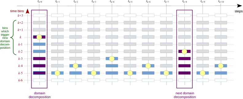
Figure 29: Sketch of the relation between work-load balancing and local time integration schemes. Filled rectangles mark the timebins that are occupied by particles. At each step of the simulation code, a certain number of timebins are synchronized, and the corresponding ‘active’ particles require force calculations. Usually, the particle count of this active set (which is the union of all synchronized timebins) is dominated by the highest synchronized timebin, which is marked with circles in the sketch. As the code hops from step to step (i.e. from $t_{n}$ to $t_{n+1}$, $t_{n+2}$, etc.), the set of active bins (marked in blue and red) and the corresponding particle configuration changes strongly, such that each step poses different work-load requirements for an optimum domain decomposition. But since the low timebins are typically thinly populated, it is often not efficient to carry out a full domain decomposition for each of them. We therefore select a subset of the higher timebins, and only carry out a domain decomposition if at least one of them is active at the current synchronization time. In such a case, the corresponding domain decomposition (such as the one at $t_{n}$) should however ‘think ahead’, and also balance subsequent steps to the extent possible, until the next decomposition will be carried out (which is anticipated for $t_{n+8}$). The decomposition therefore needs to seek an optimum compromise for balancing the steps corresponding to cases where the highest active timebins are marked in red, taking into account also the number of times they will need to be executed until the next domain decomposition is carried out.

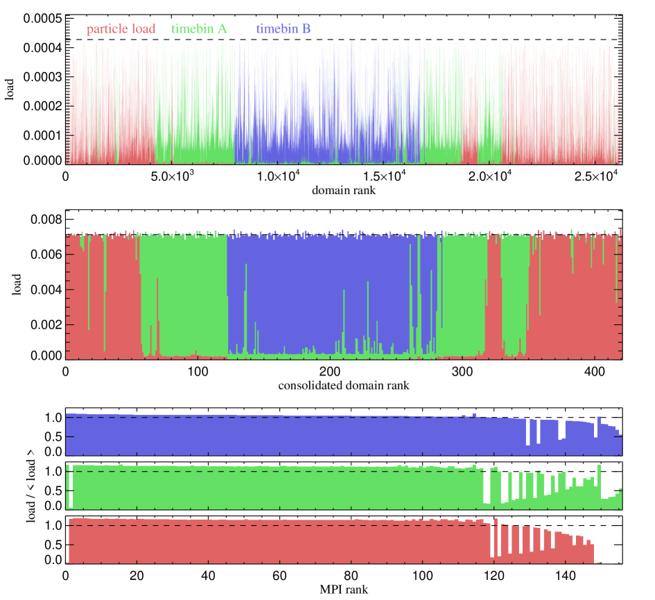
Figure 30: Real-world example of the domain balancing algorithm, here operating for two timesteps deep in the timestep hierarchy of an aggressive cosmological zoom simulation. The red colour represents the cost factor ‘particle load’, while the green and blue colours represent the computational cost of two different timebins that should be balanced simultaneously together with the particle load. In the top panel, we visualize the result of recursively subdividing the volume into about $\sim 2.5\times 10^{4}$ fine segments along a Peano-Hilbert curve that traverses the simulation volume, corresponding to the outcome of the first step in GADGET-4’s domain decomposition algorithm (the dashed vertical line marks the limit imposed for the maximum allowed combined load of the three cost items in each domain piece). These pieces are visualized in the graphics as small vertical columns of height proportional to the cost factors, and with a rank number (used as horizontal coordinate) assigned along the spatial Peano-Hilbert curve. We see that some pieces have many particles (red) but produce little or no computational load for the active timebins (green and blue), or vice versa. In the next step, the algorithm consolidates adjacent domain pieces into bigger chunks of approximately equal total load. We here have $f_{\rm mult}=3$ (since there are three cost factors), $N_{\rm cpu}=156$, and $N_{\rm extra}=47$ (the code tries different values for $N_{\rm extra}$ but we here only show the one eventually adopted because it yields the best final result). The outcome of this step is shown in the middle panel, with the horizontal line now showing the targeted average load equal to $f_{\rm mult}/(f_{\rm mult}N_{\rm cpu}-N_{\rm extra})$ for these consolidated domain pieces. These $N_{\rm domain}=421$ domain pieces (each a single segment of the Peano-Hilbert curve) can still be either dominated by particle load, one of the timebin costs, or a combination thereof. Finally, in the third step, these domain pieces are mapped to the actual number of MPI ranks by combining several in such a way that each of the cost items is very close to be balanced individually (bottom three panels). The critical measure is here that the maximum cost or load assigned to any given MPI rank should not be much larger than the average cost or load for a uniform distribution among the ranks. If needed for an acceptable compromise, the algorithm may also opt to assign fewer domain pieces to certain MPI ranks than to others, as seen on the right of the the bottom panels. Importantly, however, none of the MPI ranks exceeds the average cost in any of the three categories (i.e. force calculation cost for two different timebins, and total particle load) by more than $\sim 18\%$ or so, representing a good balance given the extreme spatial inhomogeneity of the particle load, and even more so the computational cost, in this example.

For constructing the domain decomposition, we adopt an algorithm with three stages. In the first stage, we use an oct-tree covering the simulated volume to identify a set of cubical nodes that tessellate the simulated volume. The leaf nodes of this “top-level tree” do not necessarily need to be all of the same size, instead they are selected such that each amounts to at most a certain maximum computational load (how this load is defined and measured will be discussed further below). In stage two of the algorithm, we then consolidate the leaf nodes into a set of domains, each consisting of several leaf nodes that are adjacent to each other (because they are forming a consecutive piece along the Peano-Hilbert curve that wraps through the simulated volume). This is done to arrive at domains that all have a reasonably similar total load, but which are still allowed to have different characteristics in terms of whether they are dominated by memory- or work-load, or from which timebins their work-load is mostly created. Multiple timebins need to be balanced when the domain decomposition is not newly carried out for every single step, but instead is retained for a sequence of sequential steps that traverse the timestep hierarchy, as illustrated in Figure 29. Also, for force computations in the hierarchical time integration scheme, it is desirable to balance multiple timebins all at once in a single domain decomposition. Since the depth and relative occupancy of the timestep hierarchy often varies strongly throughout the simulation volume, simultaneously balancing different timebins is generally not possible by just using simply connected regions in the domain decomposition, but it can be attained by combining pieces from different regions on the same CPU. This is why we map these domains in the third stage of the algorithm to the (smaller) set of MPI ranks. This mapping allows a balancing of multiple criteria in a jigsaw style fashion all at once. We now describe these three stages in turn.

6.1.1 Creation of leaf nodes for the top-level tree

Let $q_{i}$ be a gravitational cost factor associated with particle $i$, meant to be a proxy for the CPU-time needed to compute the tree- or FMM-based gravity calculation for this particle on the CPU it resides on. We simply approximate this with the number of multipole interactions the particle experiences in its gravity calculation, as measured for its last force calculation. We can then define a total cost factor for an oct-tree node $j$ and timebin $b$ as

$$g_{j}^{b}=\sum_{\begin{subarray}{c}i\,\in\,{\rm node}\,j\\ i\,\in\,{\rm timebin}\,b\end{subarray}}q_{i}.$$ (101)

where only particles are counted that are active on bin $b$. The total gravitational cost that should be balanced by the domain decomposition for timebin $b$ can hence be characterized by

$$\tilde{g}^{b}=\sum_{j\,\in\,{\rm leaves}}g_{j}^{n}$$ (102)

where the sum extends over the leaf-nodes of the tree, which tessellate the simulation volume. We are further defining a total cost factor $K_{j}$ of a leaf node as

$$K_{j}=\frac{N_{j}}{N_{\rm tot}}+\sum_{b\,\in\,{\rm active\,bins}}w_{b}\frac{g_{j}^{b}}{\tilde{g}^{b}},$$ (103)

where $N_{j}$ is the particle number in node $j$, and $N_{\rm tot}$ is the total particle number. The sum over the bins goes here over the set of timebins the domain decomposition is supposed to simultaneously balance, along with the particle load, which is always included. The meaning of the weight parameter $w_{b}$ will become clear later on.

The construction of the top-level tree in stage one is now done iteratively. At each iteration, all leaf nodes with load $K_{j}$ above some threshold $K_{\rm max}$ are refined into 8 daughter nodes, replacing these leaves. As limiting threshold we pick

$$K_{\rm max}=\frac{1}{f_{\rm top}f_{\rm mult}N_{\rm CPU}},$$ (104)

where $f_{\rm mult}$ is set equal to the number of different cost categories we want to balance (so if two timebins are active, we would set $f_{\rm mult}=3$, because we also have the particle load), $N_{\rm CPU}$ is the number of MPI ranks for which we want to reach the balance, and $f_{\rm top}\simeq 2-5$ is a parameter that can be varied to make the decomposition finer if desired. Note that the sum over the leaf nodes represents a disjoint partitioning of the full particle set, i.e. the sum of the corresponding loads of the domains will be

$$K_{\rm tot}=\sum_{j\,\in\,{\rm leaf\,nodes}}K_{j}=1+\sum_{b\,\in\,{\rm active\,bins}}w_{b}.$$ (105)

Our goal with this subdivision is to obtain a sufficiently fine set of leaf nodes such that their load in each cost category is less than $K_{\rm max}$.

However, if a timebin is sparsely loaded, this may become impossible to achieve if the number of particles is of order $f_{\rm top}f_{\rm mult}N_{\rm CPU}$ or less. Then there are simply too few particles to achieve a balanced decomposition for the number of cores. To cope with this situation, we use the weight factors $w_{b}$. We first determine

$$g_{{\rm max}}^{b}=\max_{i\,\in\,{\rm timebin}\,b}q_{i},$$ (106)

and then set

$$w_{b}=\min\left(1,K_{\rm max}\frac{\tilde{g}^{b}}{g_{\rm max}^{b}}\right).$$ (107)

This means that for the normal case of well-occupied timebins, we will have $w_{b}=1$. Otherwise, the gravity cost of the most expensive particle in the bin will be reduced such that it enters with a cost $w_{b}\,g_{{\rm max}}^{b}/{\tilde{g}^{b}}=K_{\rm max}$ in its parent leaf node, so once the code has isolated this particle in a leaf node, it will not dominate the total cost.

In passing, we note that the hydrodynamic work- and particle-load can be added in a straightforward fashion to this approach. Combined with the further steps below, this then allows a simultaneous balancing of gravitational and hydrodynamic costs and loads (which can in general vary differently in space). We refrain from explicitly adding this to the equations for clarity, but have implemented this in GADGET-4, adopting the approximation that each SPH particle requires a similar interaction count for its density and hydrodynamical force calculations.

6.1.2 Consolidation of leaf nodes into domains

We next exploit a spatial Peano-Hilbert ordering of the leaf nodes that effectively puts them into a one-dimensional list of nodes. Segmenting this list of nodes into $N_{\rm domain}$ pieces by introducing $N_{\rm domain}-1$ cuts then creates small groups of spatially adjacent leaf nodes that are characterized by a small surface to volume ratio. The cuts are done such that the total load of each group of leaf nodes is as even as possible. Since we know the cost $K_{j}$ of each leaf node from above, as well as their total cost $K_{\rm tot}$, this consolidation into equal pieces of cost $\simeq K_{\rm tot}/N_{\rm domain}$ can be achieved with good accuracy by simply considering the cumulative cost function along the Peano-Hilbert curve and carrying out corresponding cuts. Note that the factor $f_{\rm top}$ influences the average number of leaf nodes available per domain, and thus the degree to which the grouping procedure can smooth out the residual unevenness in the load distribution of the leaf nodes.

Using directly $N_{\rm domain}=N_{\rm CPU}$ in this approach will however not necessarily yield good results when the computational cost associated with individual particles varies strongly within the computational volume. In particular, it would then not be possible in general to balance both memory-load and gravitational work-load well at the same time, because the distribution of particles onto the timestep hierarchy as well as the particle clustering (which influences the gravitational cost factors) will typically show substantial spatial variations, with some timebins being active only in small subsets of the particle distribution. This means that a good balance in all of these different cost categories can not be constructed if only simply connected regions are used.

6.1.3 Mapping domains to processors

To improve on this, we therefore use a third stage in our domain decomposition algorithm. This starts with the idea to combine several domains of different load characteristics on a single processor, with the intention to average out the unevenness in their relative load characteristics. Because all domains after stage two above have constant total cost, an uneven distribution in the particle load implies that there must be an uneven distribution in the gravitational cost as well. It thus should be possible to combine a domain which has many particles but low gravitational cost with one that has few particles and high gravitational cost, achieving something that is fairly balanced overall. This forms the basic idea.

We realize this approach with a heuristic algorithm that mimics how one may perhaps pack a set of moving boxes. Here, a common strategy is to first place the biggest item left into an empty box, and then combine it with the largest remaining item that still fits in. Using this as a guiding principle, we sort the domains in order of decreasing load in each cost category. We then pick the next empty processor, assign the domain with the most uneven cost that is left, and then sift through the other domains that are most unevenly loaded according to the other cost items and see whether they still fit in. Since we want to balance $f_{\rm mult}$ different cost items, we expect that $N_{\rm domain}=f_{\rm mult}N_{\rm CPU}$ may be a good starting point, with the idea to then combine $f_{\rm mult}$ domain pieces on a single processor.

However, enforcing a fixed number of domain pieces per processor is inflexible and makes the approach prone to worst case outliers. Because at the end of the day, it unfortunately does not help at all if almost all of the processors have a very uniform load, apart from one exception that deviates and has a significant excess. If, for example, this one processor has a load that lies 50% above the average, then it will hold up all other processors, independent of their number, creating a lever arm for losing a huge amount of CPU time. So the figure of merit is to make the imbalance

$$B=\frac{\max L_{i}}{\left<L_{i}\right>}$$ (108)

for each of the cost items as small as possible, where $L_{i}$ is the load of a particular cost item on CPU $i$.

To avoid becoming dominated by unwieldy domains that do not fit well with others, we instead use the ansatz

$$N_{\rm domain}=f_{\rm mult}N_{\rm CPU}-N_{\rm extra},$$ (109)

with $N_{\rm extra}$ being some number between 0 and $N_{\rm CPU}$. This would for example allow us to put $f_{\rm mult}$ domains onto $N_{\rm CPU}-N_{\rm extra}$ cores, and $f_{\rm mult}-1$ domains on the remaining $N_{\rm extra}$ CPUs. While this will induce an imbalance of at least

$$B_{\rm min}\simeq\frac{f_{\rm mult}N_{\rm CPU}}{f_{\rm mult}N_{\rm CPU}-N_{\rm extra}},$$ (110)

it may nevertheless allow for a better packing solution than for the case $N_{\rm extra}=0$, simply because we have now the freedom to leave some problematic domains from the tail of the distribution paired with no or fewer other domains.

To pick a nearly optimum solution, we use the following algorithm. For a given value of $N_{\rm extra}$, we first carry out stage two of the above algorithm to obtain a set of domains with balanced total cost. We then select a fiducial load threshold

$$l_{\rm max}=\frac{B_{\rm thresh}}{N_{\rm CPU}},$$ (111)

starting with $B_{\rm thresh}=B_{\rm min}$. We stop packing a processor with further domains when we cannot avoid filling it above this maximum load for any of the cost categories that we want to balance simultaneously. If this happens, we move to the next empty processor. It can now happen that we run out of processors before we have distributed all domains. In this case, we have aimed for a too aggressive $l_{\rm max}$. We therefore try again by allowing for a larger value of $B_{\rm thresh}$. Furthermore, we may retry the whole packing procedure for different values of $N_{\rm extra}$.

In practice, we carry out all these trials in parallel, with each processor evaluating a different trial mapping that tests a binary tuple $(N_{\rm extra},B_{\rm thresh})$. This allow us to then adopt the solution that yields the smallest overall imbalance value $B$.

In Figure 30, we show an example of the outcome of this complex domain decomposition algorithm, here carried out with two lower timebins in a high-resolution zoom simulation of a dark matter halo. For definiteness, we pick the Aq-A-2 halo of the Aquarius project, and consider it around $z\simeq 0$. There are $6.07\times 10^{8}$ particles in total in the simulation box, which is relevant for the load balancing. Only a subset of $1.85\times 10^{7}$ is active in timebin A, and far fewer still, $6.92\times 10^{5}$, in timebin B. These timebins are populated by particles in the centre of the halo the simulation is zooming on, and occupy only an extremely small region of the full volume of the simulation box. Making a spatially disjoint subdivision of space such that each processor gets roughly an equal number of particles in total, and has equal particles in timebin A as well as timebin B is rather challenging. As the figure illustrates, GADGET-4’s domain decomposition algorithm is nevertheless reasonably successful in this. It pushes down the maximum relative imbalance in any of these three cost categories to about $18\%$ in this example.

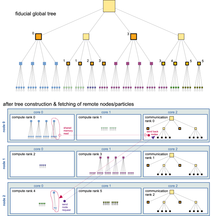
Figure 31: Organization of parallel tree calculations in GADGET-4 using a hybrid MPI/shared-memory parallelization approach. The fiducial oct-tree sketched in the top half covers the full simulation domain and contains all its particles. It is comprised of a ‘top-level’ tree that is constructed in the domain decomposition and which ends in a set of leaf nodes, marked with bold borders. The leaf nodes form a non-overlapping tessellation of the simulated volume and are mapped to individual compute ranks, as indicated by the digits 0 to 5 in the sketch. In the example, the code runs on three compute nodes with three cores each. In total six compute ranks remain, because on each of the nodes, one core is set aside to act as a communication rank and for holding a local copy of the top-level tree. All branches below the top-level leaves are stored initially without redundancy on the compute ranks. If a compute rank needs further branch data from a remote node (because it wants to open the node), this data is fetched from the corresponding remote node and integrated into the tree on the local node. In the sketch, this is indicated by compute rank 4 needing a node and its children from a branch stored by compute rank 0. To get it, rank 4 sends a request to the dedicated communication rank of the shared-memory node on which compute rank 0 resides, as sketched. The corresponding communication core constantly listens for incoming requests. It attends to an arriving message immediately by reading the requested data from compute rank 0 via a shared memory access (independent of whether or not rank 0 is busy with calculations) and sends it back to compute rank 4. There, it becomes available not only to the originally requesting rank, but also to all other compute cores on the same node (e.g. rank 5 in the example).

6.2 Hybrid parallelization

The number of compute cores on powerful supercomputers is growing rapidly, and much of their performance increase nowadays comes from a larger number of cores, not an improved single core performance. Unfortunately, subdividing a given problem size over an ever larger number of MPI ranks becomes rapidly difficult. This increases the cost for the domain decomposition algorithm, amplifies work-load imbalance losses, and may expose problems of scalability in the MPI software stack itself, for example if memory consumption for MPI buffer spaces grows faster than linear in the number of ranks, causing an eventual depletion of the memory left for the science application.

In this situation it can be advantageous to combine shared-memory with distributed-memory parallelization. One idea is to place only one (or a few) MPI ranks per multi-core compute node. The memory of the node is then used in full by the MPI rank’s process, running on a single core, and the other cores are utilized with parallelization techniques for shared memory. This can, for example, be done through code that explicitly implements multi-threading with the pthreads library. Alternatively, one can use compiler extensions introduced by the OpenMP standard, which has become a widely available technique on current platforms.

In practice, the combined use of MPI and OpenMP can reduce the number of required MPI ranks to reach a given total memory size and core number. It can also help to reduce work-load imbalance losses, limit redundancies in data storage, and lower overhead due to the MPI software stack. However, despite these advantages, it can often be difficult to reach the same or a higher raw speed with MPI+OpenMP compared with a pure MPI code for the same number of cores. For example, Lee et al. (2021) recently reported results for a new hybrid MPI-OpenMP version they developed for the RAMSES code, reaching a speed-up of a factor of 8.5 when 64 threads are used on nodes equipped with Intel Xeon Phi 7250 68C many-core processors. This is still far from the theoretical speed up of 64 that one may expect if each core was running its own MPI process and perfect parallelization was achieved. One reason lies in cache-utilization and memory access patters. Because the OpenMP threads are not isolated from each other, one needs to avoid that they interfere with each other’s cache lines in write operations, that they access memory banks attached to remote sockets on the same node, and that they spend a lot of time in congested locks, otherwise very significant performance losses can result. A more subtle problem can arise when one requires strict reproducibility of simulation results when the same run is repeated with the same setup, as this prevents the use of elementary OpenMP reduction operations that compute sums of floating point numbers in an unspecified order.

Another difficulty is that all routines that consume relevant amounts of CPU-time need to be very efficiently parallelized with OpenMP, otherwise the additional cores occupied by the OpenMP threads are only partially utilized, limiting scalability. In simple cases, the required OpenMP parallelization can be accomplished by annotating the serial code with compiler pragmas that guide loop-level parallelization done by the compiler. However, in less trivial cases (which is unfortunately the common situation in GADGET-4) code rearrangements or algorithmic changes are also required to make this really effective. One then faces a double challenge of parallelization; one needs to devise an algorithm amenable to very good distributed memory parallelization, which on top can be further parallelized well at the loop-level or through task-based algorithms.

After pursuing this OpenMP approach for some time with mixed success (our implementations worked extremely well for our tree-based gravity and SPH calculation loops, but much less well for PM- and FMM-gravity, as well as auxiliary code parts such as the domain decomposition and the group finding algorithms), we eventually abandoned it for another shared-memory parallelization strategy that we describe in the following. An important motivation for this was primarily that the OpenMP ansatz does not help at all with the need to parallelize across distributed-memory compute nodes – this remains to be addressed by MPI. And here our communication algorithms were still suffering from losses due to insufficient synchronization, i.e. when an MPI rank wanted to fetch remote data from another process, it would often have to wait for this other process to call an MPI function – only then the message exchange could proceed.

We have first tried strategies like asynchronous communication or MPI’s one-sided communication routines to mitigate these problems, but only with limited success. A central problem proved to be that most existing MPI libraries do not really guarantee asynchronous progress of MPI message exchanges while the cores are busily executing computational loops. In practice, this severely impairs the idea to overlap communication and computation, and makes the performance achievable with hardware-assisted remote memory access (RMA) highly system dependent. Disappointingly, while one-sided communication relying on the new functionality embedded in MPI-3 is fully portable, the performance achieved with this is not (e.g. Schuchart, Kowalewski & Fürlinger, 2018), simply because RMA accesses are not possible on all systems with similar performance, or are implemented by the MPI libraries in very different ways that require different, library-dependent optimization strategies.

To address this in a different way, we are using in GADGET-4 a new feature of MPI-3, which allows the allocation of shared memory that can be jointly accessed by the MPI ranks residing on the same shared memory node. This allows the possibility to replace MPI send- and receive-operations within a compute node by direct read and write memory accesses using shared memory semantics, thereby effectively allowing true one-sided communication within a shared memory node that does not require any immediate cooperation of the other process.

We extend this concept to multi-node runs by setting aside one MPI rank on each node to be solely responsible for dealing with one-sided communication requests. When an MPI-rank wants to access remote data on another MPI-rank on a different compute node, it does not send a communication request directly to the target rank, but instead to the target node’s designated communication rank, which then fetches the data via a shared memory access (the target rank’s process doesn’t have to cooperate for this, i.e. this is readily possible even if the process is busy doing computations) and relays it back as needed. Since the designated communication rank is doing nothing but constantly waiting for such incoming requests, they can be answered with minimal latency. This eliminates the synchronization losses in our core computational algorithms we alluded to above, whereas OpenMP parallelization only managed to somewhat reduce them by lowering the number of MPI ranks that are in use.

The price one pays for this that at least one core per node needs to be set aside for handling the MPI communications in this form. Typical HPC systems now have often $\sim$24 – 64 cores per node, with a clear trend towards further growth of this number. This means that only a few percent of the raw performance have to be set aside for the communication rank, which appears insignificant if this yields an overall faster and more scalable code. We note that this way of doing MPI-based shared memory programming also allows other important savings, like storing data that is equal on all MPI-ranks (e.g. the top-level tree, or large look-up tables) only once per compute node, and not for all MPI ranks separately.

6.3 Data layout and communication scheme in parallel tree walks

In Figure 31, we sketch how GADGET-4 uses the above concepts for organizing its parallel tree-based calculations. The top-level tree constructed in the domain decomposition is equal for all the MPI-ranks in a shared-memory node. It is hence only stored once on each shared-memory node (we use the memory associated with the dedicated communication rank for this, but one of the compute ranks could also be used). The compute ranks only store the tree branches assigned to them by the domain decomposition, without redundancy. When the tree is walked, each MPI-rank can freely access all nodes from the top-level tree, its own branches, as well as those of the other MPI-ranks on the same compute node, via shared-memory accesses. If an MPI-rank needs to open a tree node whose daughter nodes or particles are stored on a remote compute node, this data is fetched from the remote node by contacting its designed communication rank, which then returns the requested data with minimal latency, side-stepping the MPI-synchronization losses mentioned above. We however still buffer such node-requests and accumulate them into larger packages to avoid creating a large number of tiny messages. Imported node data augments the locally stored tree, and becomes immediately accessible also to all other MPI-ranks of the same shared-memory node. After all tree walks are carried out by them, the locally held tree data thus corresponds to a “locally essential tree” (which is a subset of the fiducial global tree) needed to fully carry out the tree walks of all particles mapped to the local shared memory node.

We note that one side-effect of the buffering approach mentioned above can be that it breaks the deterministic outcome at the binary floating point level, which is undesirable as discussed earlier. This can happen when a tree walk is continued despite a node’s children need to be fetched. Instead of waiting for arrival of the data, the node interaction may be temporarily cached and revisited later once the data has arrived. However, another MPI-rank may have been quick enough and already imported the node’s children, in which case the tree walk would have been able to continue right away by opening this node, altering the order in which the partial contributions are added up. A tell-tale sign that this type of problem can occur is that the insertion of imported nodes into the locally held tree needs to be protected by a spin-lock to avoid a data-race condition.

However, binary invariance can be easily re-established by carrying out the actual tree calculations only after the locally essential tree has been fully assembled. This requires a slightly higher computational cost as it entails some tree-walking overhead in the form of repeated evaluations of node-opening decisions, and is thus made an optional feature in GADGET-4.

Note that the concept of constructing a locally essential tree, which is followed by GADGET-4 here and has been previously adopted by other tree codes (Dubinski, 1996), is notably different from the communication strategy adopted in previous GADGET versions, where instead of importing remote branch data to process a local particle the particle was sent to the MPI-rank holding the remote branch, which would then do the computational work and send back the result. The latter approach works well for TreePM and SPH, where the interactions are limited to a small neighbourhood around the local domain, but it has a less favourable scaling behaviour with respect to the data volume that needs to be communicated when a pure Tree or FMM approach are used. Its main downside is that remote processes need to actively contribute computational cycles to processing local particles – getting them to do that requires synchronization of some kind, creating ample opportunity for parallelization losses due to wait times. On the other hand, the memory requirements of the locally essential tree approach can become very challenging in the limit of tiny opening angles. If the opening angle is approaching zero, the final locally essential tree becomes ever closer to the fiducial global tree holding all particles, i.e. then each node would have to hold the full global tree. However, as in this limit the force-calculation degenerates to a direct summation algorithm anyhow, this is fortunately not a particularly relevant limitation for practical applications.

6.4 Parallel FFT calculation

For the PM calculations in GADGET-4, we use real-to-complex and complex-to-real discrete fast Fourier transforms in 3D. The work and memory need of such transforms scales rapidly as $N_{\rm grid}^{3}\ln(N_{\rm grid}^{3})$. In GADGET-2, the transforms were implemented using the FFTW-2 library. This library has since been deprecated and replaced with FFTW-3, which features a different application interface and some slight improvements. Both versions of the library use a slab-based decomposition for distributed memory parallel FFTs. This does not allow the efficient use of more MPI tasks than there are grid slabs, hence scalability is strictly limited to the regime $N_{\rm cpu}\leq N_{\rm grid}$. This is very problematic for today’s problem sizes in cosmology. Because FFTW-3 also uses additional internal memory allocations in its distributed transforms (something we seek to avoid to have full control of the application memory), we have developed our own version of 3D parallel FFT routines based on FFTW-3’s one-dimensional FFTs.

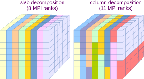
Figure 32: Slab-based versus column-based data decomposition for distributed 3D FFTs in GADGET-4. If the number $N_{\rm grid}$ of slabs is a multiple of the number $N_{\rm cpu}$ of MPI ranks, a slab-based decomposition is a good, balanced choice (as in the example sketched on the left). However, this limits the scalability of the code, particularly for large problem sizes. If the number of MPI ranks is much larger than $N_{\rm grid}$, a more flexible decomposition is needed. GADGET-4 implements a column-based decomposition where the total number of columns (typically $N_{\rm grid}\times N_{\rm grid}$ for cubical transforms, but the three dimensions may also be different), is distributed as evenly as possible among the MPI ranks, thereby greatly enlarging the scalability regime. There are no restrictions on permissible numbers $N_{\rm grid}$ and $N_{\rm cpu}$, i.e. also odd choices are readily possible, such as $N_{\rm grid}=8$ and $N_{\rm cpu}=11$ shown in the sketch on the right (different color shades refer to different MPI ranks).

To extend the range of scalability of the PM calculations, we allow both for a slab-based or alternatively for a column-based distribution of the data cube, as sketched in Figure 32. We allow for an arbitrary number of MPI ranks in relation to the grid size, and the number of columns assigned to each CPU is made as even as possible to guarantee an optimum memory balance. In particular, this means that the set of columns assigned to a MPI process does not need to have a rectangular footprint in the $N_{\rm grid}\times N_{\rm grid}$ grid. Note, however, that the column-based approach requires two global transpose operations per FFT, even allowing for a different data layout in the result, whereas the slab-based approach (which we also support) needs only one. Because the data shuffling of these transpose operations is often the dominating part of the distributed memory FFT algorithm, it is more efficient to use the slab-based approach in the regime where this still scales reasonably well. We note that the final result of our FFT algorithms is binary floating point invariant with respect to whether the slab-based or column-based version is used, and to what number of MPI ranks is employed. The code is also general enough to allow different grid dimensions in each spatial dimension, so we can employ it for stretched boxes as well.

We support two different communication algorithms to map the particle data to a density grid, and to bring back the forces to the particles. One of them is designed to be ideal for homogeneously sampled boxes. Here the particle coordinates and masses are sent to the processor holding the target column/slab, and this CPU then does the binning work. For a zoom calculation, this would become fairly imbalanced as the vast majority of particles is concentrated in a tiny volume in this case, which may fall largely onto just a single processor’s slab or column. If this MPI rank had to do all the binning work, it would form a parallel bottleneck. To rectify this, GADGET-4 offers an alternative approach that is optimized for this scenerio. In it, each processor bins the particles to local grid cells of the density field (just those that are actually touched), and then only the resulting density values are sent to the right target processor where they are assembled to the complete density field.

6.5 Generic parallel tree walks

There are a few places in GADGET-4 where parallel tree walks are needed that are not best addressed by building a locally essential tree, but rather by exporting a particle to the MPI-rank holding a required remote tree branch, which then carries out the remaining walk there and reports the result back, where it can be accumulated. This is for example the case in our FOF group finding algorithm to connect up groups that stretch across domain boundaries, or in the spherical overdensity method to measure virial masses of halos by determining the enclosed mass in large spherical apertures. It can also be useful for certain types of feedback algorithms that spread energy (or metals) from an SPH particle to its neighbours.

All these tree walks can be realized with the same generic communication pattern. First, the code starts on each MPI rank with walking its active particles. This accounts for all local interactions, but some tree branches cannot be opened. This fact is noted in an export buffer, together also with the exact information at which tree node the local walk could not be continued. Once all local particles have been processed (or the export buffer is full), the particle coordinates and foreign node addresses stored in the export buffer are sent to the corresponding target processor, while the local processor itself receives incoming requests of the same kind. After this data exchange, which is normally carried out with a robust hypercube pattern with pairwise synchronous data exchange, branches of the local tree are walked to produce partial results, which are then sent back to the originating process and added in to the local results. If needed, the cycle is repeated until all active particles are processed.

Compared to older versions of GADGET, the newly implemented approach of this generic pattern in GADGET-4 is more efficient because it includes the index (or several indices) of the starting node of the partial tree walk required on the foreign processor, instead of finding this by starting again from the root node. This means that the actual tree-walking cost is invariant when the number of CPUs is changed. We also automatically use all available memory for the export buffer in a robust way, without a need to specify the size of this buffer explicitly. Furthermore, we have encapsulated the communication routines in a C++ class that puts them completely out of view in the core routines of the code. This makes it much easier to verify and modify these core routines.

6.6 Vectorization

Modern CPUs offer increasingly powerful vector instructions (such as the SSE2, AVX, AVX2, AVX512 instruction sets introduced by Intel) where several arithmetic operations can be executed in parallel through a single instruction. Reaching a substantial fraction of the peak performance of these CPUs requires extensive use of vector instructions. One approach to employ them is to rely on the ‘auto-vectorization’ features of modern compilers, which try to identify opportunities to emit vector instructions in code that is formulated with a serial syntax. Unfortunately, this does not work very effectively in GADGET-4, due to its complicated and irregular memory access and calculation patterns. Better results require a rewrite of the code with vectorization in mind. One effective way to ensure use of the vector instructions is to inline low-level vector intrinsics (which are essentially machine instructions expressed as small C functions or macros) directly in the code. In order to maintain better readability and portability of the code, we prefer to encapsulate vector intrinsics through the C++ vectorclass library. It defines new vector-sized data types and uses meta- and template programming techniques to allow the writing of fully vectorized code using the syntax or ordinary code. As an additional benefit, this allows the compilation of vectorized code on platforms that, e.g., feature different vector lengths or only support SSE2, because the meta-programming of this library can automatically replace long vector instructions with multiple short ones if only those are available.

As a demonstrator and test of the potential of this approach we have created an alternative version of the innermost SPH-loop for the density and the hydrodynamic forces based on the vectorclass library, targeting 256-bit wide AVX instructions where 4 double precision operations can be done in parallel. Our approach in this compute kernel has been to always work on four neighbour particles in parallel, applying exactly the same operations to each of them. One complication in this is the evaluation of the standard cubic SPH kernel, which involves branching due to its formulation in terms of piece-wise polynomials. We here compute both versions and then mix them using vectorized comparison and select operations. This is not necessary for the Wendland kernels, which is helpful for a more efficient vectorization (see our timings in Section 8.4). We follow a similar approach in the calculation of the artificial viscosity, which we compute for every particle and then use a select operation for deciding whether we really want to apply this term.

Compared to the ordinary serial version of the same routine (which is still available in the code and used as default) we have only reached a very modest speed-up of order 5-10% on a compute cluster with Intel Xeon Gold 6138 CPUs (which are in principle capable of AVX512 instructions). This is certainly less than what one may have (perhaps naively) hoped for. It remains to be seen whether this is due to limitations in our particular approach that can be overcome with more clever coding, or whether it rather reflects the principal difficulty to get high floating point throughput with SIMD instructions in situations where scattered data needs to be fetched from memory, and only few floating point operations are done per data item read from memory, because this is unfortunately the regime of our SPH loops. Furthermore, there can also be subtle side-effects due to the use of AVX instructions, such as an associated temporary reduction of the clock frequency of the executing core directly after such instructions.

We note that other authors have also reported somewhat mixed results when explicitly using SIMD instructions in N-body codes. Kodama & Ishiyama (2019) have used the AVX2 instructions (in assembly) to accelerate the evaluation of tree interactions with quadrupole moments in an extension of the Phantom-GRAPE (Tanikawa et al., 2012, 2013) library for calculating gravity in N-body systems, finding speedups relative to the pseudo-particle method of the library by factor of 1.1. For the use of AVX-512 they estimate a speed-up of 1.08. This appears similar to our results here. On the other hand, Ishiyama, Nitadori & Makino (2012) describe a rather successful SIMD based parallelization of the inner force loop of their TreePM code for the K-supercomputer, and Yoshikawa & Tanikawa (2018) report good performance gains with AVX-512 for the Phantom-GRAPE library. Similarly, Potter, Stadel & Teyssier (2017) reported substantial gains in PKDGRAV-3 due to explicit optimizations for SIMD instructions.

7 On the fly analysis and other features

7.1 Parallel group and subhalo finder

GADGET-4 has a built-in Friends-of-Friends (FOF) group finder (Davis et al., 1985), an implementation of the SUBFIND algorithm (Springel et al., 2001) for finding gravitationally bound substructures in positional space in a single timeslice, and a new variant, SUBFIND-HBT, that takes past information about group membership into account. All three implementations are capable of processing very large simulations as well as high-resolution zoom calculations with extremely large particle numbers in single halos. The outputs created by SUBFIND or SUBFIND-HBT can be created either on-the-fly while a simulation is running, or in postprocessing, and they can be combined into merger tree construction if desired.

The FOF algorithm uses link-lists to organize the halos, starting out with each particle making up a group of its own. The code then finds all particle pairs with a distance smaller than a prescribed linking length $l$. In cosmological simulations, the most common choice for $l$ is to make it equal to $0.2$ times the mean particle spacing, leading to halos that are bound by a density contour that approximates the overdensity expected for virialized structures according to the top-hat collapse model. Each pair that is found with a sufficiently small distance causes the groups the two particles belong to to be linked into a joint group.

For finding neighbouring particles within a distance $l$, the code uses a range searching technique based on an oct-tree, similar to the neighbour finding in SPH. Significant speed-ups are realized by flagging tree nodes which contain only particles already in the same group, or which are small enough that all particles in the node are guaranteed to be in the same node. If a target particle encounters such a node in its neighbour search and sees at least one of the node’s particles as a neighbour, the other particles in the node need not be checked any further. Compared to reported speeds of other FOF algorithms in the literature, GADGET-4’s implementation appears to be quite fast. For example, Creasey (2018) have argued that tree-based FOF group finders would be slow, suggesting instead an algorithm based on spatial hashing. Our results do not support this assertion, as our algorithm appears to be at least as fast as the one described by Creasey (2018). Also, our method works well in parallel on distributed-memory machines (see also Roy, Bouillot & Rasera, 2014), and is efficient for the demanding regime of extreme zoom calculations. In Figure 33 we show speed and scaling measurements supporting these findings. We note that the speed of our parallel algorithm for finding FOF groups is also substantially faster than the Parallel-HOP method of Skory et al. (2010)

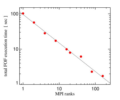
Figure 33: Raw speed and parallel scalability of the inlined MPI-parallel FOF group finder in GADGET-4. We show measurements for different numbers of MPI ranks when the algorithm is applied to the $z=0$ output of one of the lower resolution DM-only variants of the TNG50 simulation model of the IllustrisTNG project. Specifically, we here used the $270^{3}$ run with close to 20 million particles. The largest found group has about 840000 particles, and there are about 18800 groups with at least 32 particles. We have checked that the outcome of the group finder is invariant when the number of MPI ranks is changed, as required. The execution time closely follows strong scaling (solid line) over the measured range, implying a raw processing speed of around $2\times 10^{5}$ particles per second and core.

7.2 Finding subhalos with SUBFIND

When one is interested in dark matter substructures or the gravitationally bound part of halos, the FOF group finder can be combined with the SUBFIND algorithm. The latter decomposes each found halo into a set of disjoint, gravitationally bound substructures. They are identified based on an excursion set algorithm as described in Springel et al. (2001). First, the total mass density field is found by adaptive kernel estimation, allowing the identification of isolated density peaks. These density peaks are grown with an excursion set algorithm (similar to a watershed approach) until saddle points are encountered that connect two isolated density peaks. Typically the smaller peak is then registered as a substructure candidate, and is subsequently subjected to a gravitational unbinding procedure. As one improvement compared to previous versions of SUBFIND, the selection of which of the two peaks is the substructure and which is background can now optionally take into account information about previous subhalo membership of the particles making up the peaks. In the on-the-fly processing, this is done by letting each particle carry a cumulative sum of the subhalo lengths of all its previous subhalo memberships, while in the postprocessing mode of SUBFIND, the same information is gathered by processing the snapshots in their temporal order. The peak having the larger sum of all these previous sizes is then identified as the background peak, not necessarily the one with the larger particle number (typically in less than  1% of the saddle-point decisions this picks the smaller of the two peaks). A similar approach has recently also been developed by Angulo et al. (2020). This procedure substantially reduces temporal variations of the bound mass assigned by SUBFIND to subhalos, which often originate in mistakingly swapping the identity of background and substructure peaks at the saddle points. As a further side-effect, it also reduces the occurrence of swaps between central and satellite systems in the tracking of subhalos in merger trees.

The calculation of the gravitational potential in the unbinding procedure is carried out with a tree algorithm using the same multipole order and accuracy as in the ordinary force calculation of the simulation, without taking any short-cuts or additional approximations. The unbinding procedure is iteratively repeated to account for the changes in the potenial due to removal of unbound particles, and only ends when all remaining particles are bound to each other, or their number has fallen below a prescribed detection threshold for a group (typically chosen as something in the range $\sim$20-64 particles). The gravitational unbinding is also applied to the remaining “background” structure, defined as the particles left in the FOF group after all bound substructures have been extracted. Thus, every FOF halo is effectively segmented into a set of gravitationally bound subhalos, and possibly some particles not bound to any of the subhalos. The most massive of these subhalos corresponds to the ‘background halo’, also called the central subhalo, while the others are referred to as satellites. Note that sometimes the two most massive subhalos can emerge with comparable mass from the decomposition, for example in an ongoing major merger, or if the FOF algorithm has linked two nearby halos via a feeble particle bridge, making the distinction between central and satellite somewhat ambiguous.

In terms of parallelization, both FOF and SUBFIND can cope with high-resolution zoom simulations that contain groups much larger than are able to fit on individual MPI ranks. After the FOF group finder has been run, the groups are ordered by their size. If the largest group is too large to be processed by a single MPI process, it gets assigned several MPI ranks, as many as needed to fit it into their combined memory, likewise for the second group, the third group, and so on. Each such set of processes gets its own MPI communicator and works in parallel on the one halo assigned to it. Halos that are small enough to fit on individual processors are assigned in a round-robin fashion to the remaining MPI ranks, so that these MPI processes each work on several smaller halos.

If the group finding algorithms FOF and SUBFIND are used in an on-the-fly processing mode while a simulation runs, they are always executed directly before a snapshot is written to disk. This allows a convenient storage format of the timeslice data, which we output in the order of the found groups and subhalos. Any group can hence be loaded through random access to the data files, and without the need to load more data than needed. In addition, this eliminates the need to separately list membership particles in groups, for example through their IDs, and therefore reduces the required storage volume. In case SUBFIND is enabled, the particles are additionally stored within each group in a nested fashion ordered by decreasing subhalo size, and within each subhalo in the order of their binding energy. We have introduced this type of storage format first for the Illustris simulation, and refer to its public data release (Nelson et al., 2015) for further documentation. We note that if HDF5 storage of data is used (which is highly recommended), group catalogues, like all other GADGET-4 output, are stored in HDF5 as well.

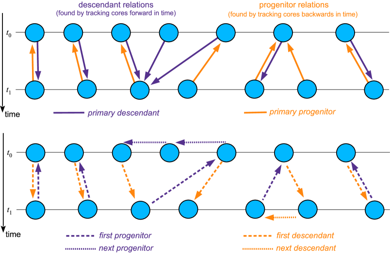
Figure 34: Descendant and progenitor relations at the stage of the linking of two subhalo catalogues. The diagram on top illustrates the fundamental tracking operation. For each subhalo, we identify a most probable primary descendant by tracking where its most bound particles end up. Additionally, we track the cores of subhalos back in time, leading to the identification of a primary progenitor. This is illustrated in the top half of the sketch. In order to be able to identify all subhalos that have a given subhalo as their primary descendant, we define an auxiliary chaining list, with a first progenitor identifying the first of these, and next progenitor links any subsequent ones, if any. Likewise, we introduce first descendant and next descendant links to be able to efficiently enumerate all subhalos that have a common primary progenitor. These induced links are illustrated in the bottom half of the sketch.

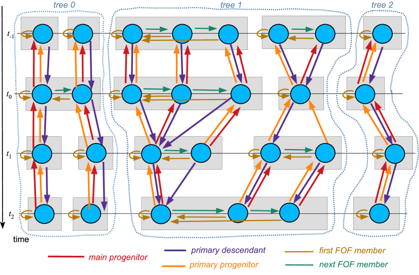
Figure 35: Sketch of the merger tree structure produced by GADGET-4. The fundamental building blocks are the primary descendant and primary progenitor links that are formed by tracking subhalo cores forward and backwards in time. These links also induce enumerations of all subhalos that are descendants of a given subhalo, which can be accessed by the first progenitor and next progenitor links shown in Fig. 34. For clarity, these links are omitted in the present sketch, but they are contained in the tree structure produced by the code. Likewise, there are first descendant and next descendant pointers that provide access to all subhalos that have a given subhalo as their primary progenitor. The tree structure also contains a main progenitor pointer, which selects the subhalo on the most massive history branch relative to the current subhalo. The chain of links established by first FOF member and next FOF member allows that each subhalo can easily enumerate all subhalos within the same FOF group (schematically indicated by the grey boxes in the sketch). For convenience, the code subdivides all subhalos into disjoint sets of trees. All pairs of subhalos that are linked via a progenitor or descendent relation, or are in the same FOF group, are guaranteed to be found in the same tree. Note that this means that a given tree can account for more than one FOF group at the final time, as seen for example in the leftmost tree 0, where two FOF halos are temporarily joined at time $t_{0}$.

7.3 Tracing bound structures with SUBFIND-HBT

The identification of gravitationally bound substructures in configuration space based on a single time-slice, which SUBFIND introduced in a fully adaptive way, is computationally demanding and can have problems in robustly identifying all matter belonging to a substructure, especially close to pericenter of a subhalo orbiting in a larger halo, as here only the densest part of the substructure sticks out over the background density field (Knebe et al., 2011; Muldrew, Pearce & Power, 2011). One approach to find this material is to look at the clustering of particles in phase-space, which prompted the development of group and subhalo finders working with the phase-space distribution. Recent examples include HST (Maciejewski et al., 2009a, b), ROCKSTAR (Behroozi, Wechsler & Wu, 2013) and VELOCIRAPTOR (Elahi, Thacker & Widrow, 2011; Elahi et al., 2019). Finding a suitable metric for distance in phase-space (to allow a 6D-FOF algorithm) is one of the central requirements for these approaches. Sometimes these methods neglect a gravitational unbinding step, making them particularly fast (akin to the FOF algorithm), but arguably at the price of a less securely defined physical nature of the identified structures. Even phase space finders are however not free of difficulties from ambiguities in the descendent identification, especially during mergers and deep encounters, causing problems in merger trees through missing or incorrect links (e.g. Srisawat et al., 2013; Avila et al., 2014).

An alternative is to rely on past information for subhalo identification. If one has somehow identified a set of particles that are gravitationally bound to each other at a given time and fall as a substructure into a bigger system, one can simply continuously check for boundedness of these particles. This assumes that a genuine substructure is only stripped of particles with time, but does not grow in mass any further in any appreciable way while on orbit in a bigger system. This is a fairly realistic approximation for the dynamics of hierarchically growing cold dark matter structures. A first realization of this idea goes back to the seminal work of Tormen, Diaferio & Syer (1998). Recently, it has been significantly refined in the hierarchically bound tracing (HBT) algorithm of Han et al. (2012, 2018).

We have implemented in GADGET-4 a variant of the HBT+ algorithm of Han et al. (2018). Because it can in practice act as a drop-in replacement for SUBFIND with identical output structure and merger tree format, we call this approach SUBFIND-HBT. It only works for a sequence of simulation snapshots that need to be processed in temporal order, i.e. to identify the substructures at any given time, our algorithm uses the known group and subhalo catalogue of the previous output time (this is either available when the algorithm is run on-the-fly, or loaded in postprocessing). The method first finds new FOF groups at the current time. Next, substructure candidates are identified within each FOF group based on the previous substructure membership of all its constituent particles. The largest substructure candidate found in this way is then discarded for the moment, because our approach identifies it with the background halo of the group, which also may grow in mass. In contrast, the other substructure candidates are subjected to a gravitational unbinding procedure, using their new phase-space coordinates. By construction, this can at most recover the mass the substructure had in the previous output, while in general, the remaining bound mass may reduce. Finally, all particles of the group not ending up still bound to any of these subhalo candidates will finally be subjected to a further gravitational unbinding procedure. Note that this particle set includes the particles that were in the biggest substructure candidate which was initially dropped. If the FOF group has grown in size, this gives the background subhalo a corresponding opportunity to grow in mass.

Compared to the ordinary SUBFIND algorithm, the approach followed by SUBFIND-HBT is evidently considerably simpler and computationally cheaper. This is because it does not have to compute an adaptively smoothed density field, and especially, these densities do not have to be processed in an inherently serial approach from high to low density to find all saddle points. Furthermore, there are no spurious subhalos that are only eliminated by the comparatively costly gravitational unbinding procedure. The main advantage of SUBFIND-HBT is however that it is capable to recover the full mass of substructures also close to pericenter on their orbit. This yields a more robust tracking of substructures, and an overall higher quality of the corresponding merger trees. The superior properties of the HBT algorithm have also been confirmed by Behroozi et al. (2015) and also show up in the results of Elahi et al. (2019). Despite the conceptional simplicity of the approach, the tracking delivered by HBT is highly robust, largely making it superfluous to fix glitches in merger trees such as those resulting from the occasional tracking problems of essentially all other substructure finding methods. We therefore expect that merger trees constructed with SUBFIND-HBT are a highly competitive alternative to other algorithms.

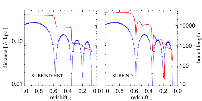
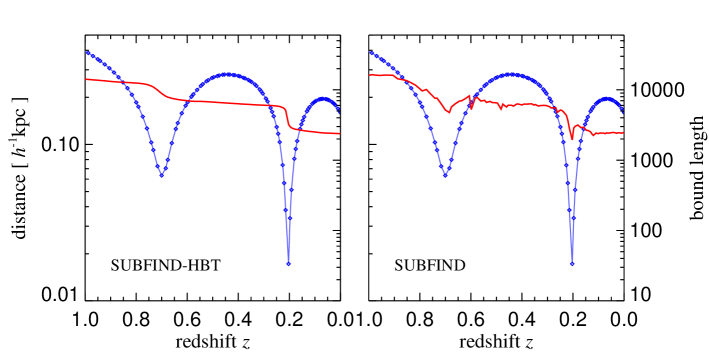
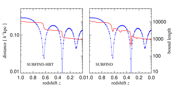
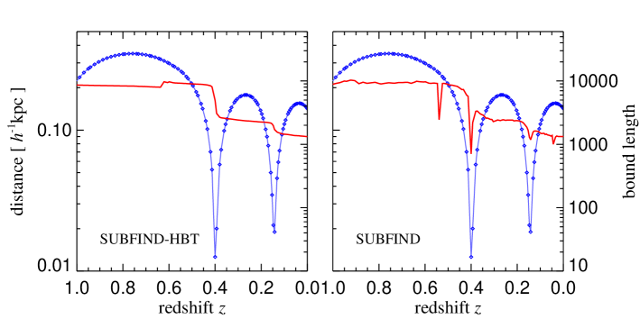
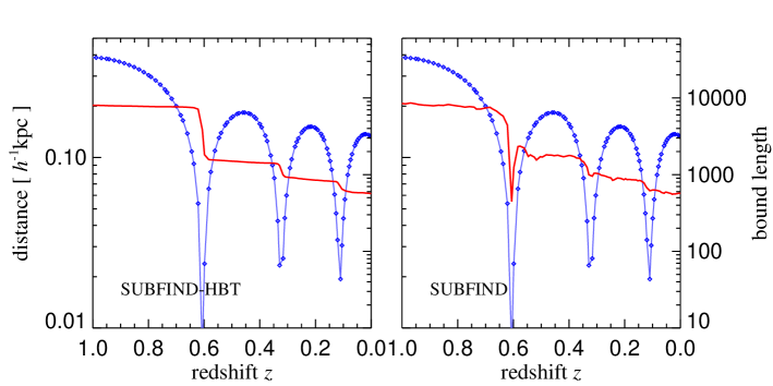
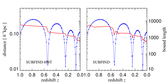
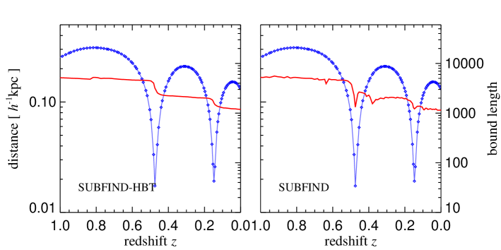
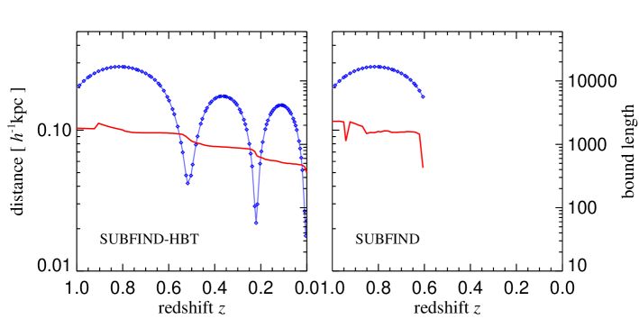
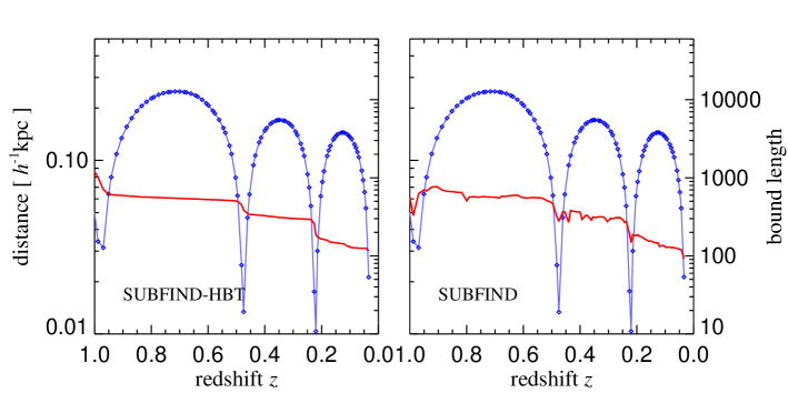
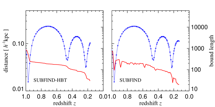
Figure 36: Comparison of the SUBFIND and SUBFIND-HBT approaches when applied to subhalo tracking forward in time, for a cosmological zoom-in simulation of a Milky Way-sized dark matter halo. For definiteness, we consider a rerun of the Aq-A-4 halo of the Aquarius project (Springel et al., 2008a), and identify halos and subhalos twice, once with the traditional SUBFIND algorithm (Springel et al., 2001) and once with SUBFIND-HBT, which is our implementation of the approach of Han et al. (2018). We select a set of 10 subhalos at $z=1$ and track their fate forward in time based on the merger tree algorithm built into GADGET-4. In each pair of panels, the same subhalo is examined, in the left it is found with SUBFIND-HBT, and on the right with SUBFIND. Blue lines give the distance to the halo centre (symbols mark the discrete output times), while the red lines show the gravitationally bound particle number retrieved by the substructure finders. One can clearly see temporary depressions of the substructure size reported by SUBFIND around pericenter passages, and in some cases the substructure tracking is lost earlier in SUBFIND than with SUBFIND-HBT. Overall, both approaches make reassuringly similar predictions for the mass loss experienced by the orbiting subhalos.

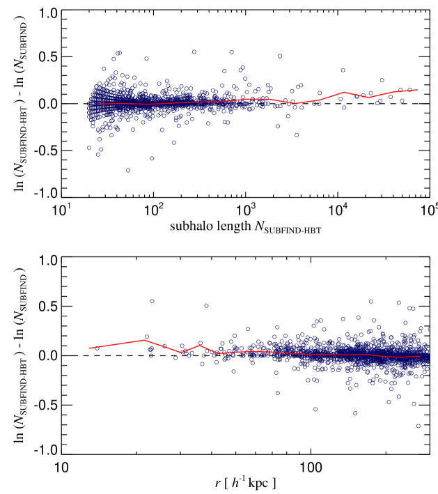
Figure 37: Comparison of subhalo sizes detected with the SUBFIND-HBT and SUBFIND algorithms, in a cosmological simulation of a Milky Way-sized halo at $z=0$ (a rerun of the Aq-A-4 simulation). The top panel shows the difference in the sizes of matching subhalos (symbols), as a function of their size, with an overplotted running median (solid red line). The bottom panel plots the same quantity, but now as a function of distance to the halo centre. On average, the sizes agree rather well, but there is a weak trend towards slightly larger sizes found with SUBFIND-HBT in the inner parts of the halo, and for the largest subhalos.

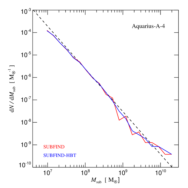
Figure 38: Comparison of the differential subhalo mass function for a re-run of the Aquarius Aq-A-4 halo with GADGET-4, using two different substructure detection algorithms, the ‘classic’ SUBFIND algorithm, and the hierarchical bound tracing method SUBFIND-HBT. For further comparison, the dashed line gives the fit to the result reported in Springel et al. (2008a). Reassuringly, the results are extremely close between the two subhalo finders, even though they detect substructure candidates in fundamentally different ways. The result is also in good agreement with the older findings in Springel et al. (2008a), based at the time on an early version of GADGET-3.

7.4 Merger tree construction

For many scientific applications, merger trees are an essential input as they give the ability to track individual halos through cosmic time. This is, for example, needed for semi-analytic models of galaxy formation that follow physical models of galaxy evolution on the dark matter backbone, and predict how galaxies populate the structures. Traditionally, merger tree building is done in postprocessing, because it involves a complex matching exercise between many simulation outputs at different times. Because all produced snapshots and group catalogues are involved, this post-processing operation is also a rather data-intensive operation. For simulation sizes that in select cases already reach over a trillion particles, this poses a serious challenge. For example, for the recent Uchuu simulation of Ishiyama et al. (2020) merger tree construction was done by splitting the simulation volume into 8000 boxes and sub-catalogues, as the calculation could otherwise not be processed with the available ROCKSTAR halo finder software. In addition, it basically has become infeasible for simulations of that size to produce a large amount of finely spaced snapshot outputs just for the sake of constructing merger trees, due to the prohibitive data volume involved.

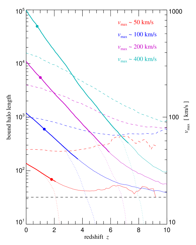
Figure 39: Backtracking of central halos selected by different maximum circular velocity at $z=0$, in a cosmological dark matter-only simulation with $648^{3}$ particles in a $75\,h^{-1}{\rm Mpc}$ box. The solid lines show the average bound particle number in the main progenitor stems of the selected halos as they are tracked back to high redshift. If a halo cannot be tracked any more, it is discarded in the averaging, that is why towards high redshift only a subset of the original halos can still be tracked, so that averages eventually become biased towards early formation times. For the thick part of the solid lines more than 50% of the halos can still be tracked, while the dotted lines show the result if the ones that cannot be tracked any more are considered in the averaging with zero length. The dashed lines give the average maximum circular velocity of the (still trackable) progenitor halos, with the corresponding quantitative scale indicated on the vertical axis on the right. The solid circles mark the times when the mass of the main progenitor has dropped to half the halo mass at $z=0$, which is a commonly employed definition of the formation time of a halo. The corresponding redshifts are $z=1.8$, $1.3$, $1.0$, and $0.8$, in increasing order of final mass for our four samples, reflecting the hierarchical growth of structure.

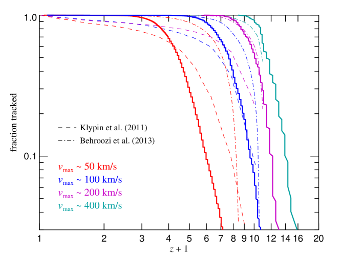
Figure 40: Fraction of holes selected at $z=0$ that can be tracked back to a given redshift (solid lines), for four different maximum circular velocity choices, as labelled. For comparison, we also show results reported by Klypin, Trujillo-Gomez & Primack (2011) and Behroozi et al. (2013), respectively, for the Bolshoi simulation, which has a very similar mass resolution (within $1\%$) as the test run considered here (with $648^{3}$ particles in a $75\,h^{-1}{\rm Mpc}$ box). Our tracking results, as well as those of Behroozi et al. (2013), clearly outperform the approach in Klypin, Trujillo-Gomez & Primack (2011). Our results also indicate an advantage over the combination of ROCKSTAR groupfinder and CONSISTENT-TREES merger tree builder of Behroozi et al. (2013) for large halos, while the opposite appears to be the case for small halos. The latter could however be simply related to our comparatively conservative minimum halo size of 32 particles.

It would thus be very helpful if the data-intensive part of the merger tree finding could already be done on the fly, making it possible to construct merger trees that are finely resolved in time without ever having to output the full particle data. In GADGET-4, we achieve this by executing FOF and SUBFIND (or SUBFIND-HBT) on the fly at a prescribed set of output times. But instead of storing raw particle data to disk, only the group and subhalo catalogues are saved, which contain information about collective properties of each group and subhalo, like mass, position, bulk velocity, spin, etc., but do not list each particle making up the group. Correspondingly, the data volume of these group catalogues is quite small. To establish the necessary links of halos in time (and hence between different group catalogues) we let the code retain membership information of each particle in a certain group and subhalo while the simulation continues. Right after a new group catalogue is determined, the membership information in the previous group catalogue is then still present, allowing us to link the group catalogues with each other. This is done similarly as first described in Springel et al. (2001), but with some notable improvements described below. After the linking information has been determined, it is output to disk (this again is very small in data volume compared with the full particle set, and represents only a minor addition to the halo catalogues) alongside with the new group catalogue. Finally, the membership record of each particle is updated with that of the new group catalogue; this will then be used when the next group catalogue at a slightly later time is computed and the corresponding links to this new one are determined.

We establish the links as follows. Let us consider two subhalo catalogues at subsequent times $t_{0}<t_{1}$, with a total number of $N_{0}$ and $N_{1}$ subhalos, respectively. Note that we use the term subhalo also for the main gravitational background halo of a FOF-group in which secondary subhalos may be embedded, as is standard nomenclature for SUBFIND. A particle can only be member of one subhalo at a given time, hence the subhalos form gravitationally bound disjoint sets of particles at a given time. Let’s assume the subhalos are numbered in some fashion, for example $0,1,\ldots,N_{0}-1$ at time $t_{0}$. For each particle $i$ that is bound in a subhalo at this time, we assign a rank $r^{(0)}_{i}$ based on ordering the particles according to increasing binding energy within the corresponding subhalo. The particle with rank $r^{(0)}_{i}=0$ is hence the gravitationally most bound particle in its subhalo. Based on the rank, we assign a score

$$S^{(0)}_{i}=\left\{\begin{matrix}\;\left[1+[r^{(0)}_{i}]^{q}\right]^{-1}&\mbox{for}\;\;r^{(0)}_{i}<N_{\rm core}\\ 0&\mbox{otherwise}\end{matrix}\right.$$ (112)

to the particle $i$, where $N_{\rm core}$ is the maximum number of most-bound particles that are used to link subhalos (we use $N_{\rm core}=16$ as our default choice), and $q$ is a parameter that influences how much more weight should be given to more strongly bound particles in the tracking (we use $q=0.5$ as our default choice and find that our results depend at most extremely weakly on this choice). Particles not bound in a subhalo are assigned a zero score. In an analogous fashion, we assign scores $S^{(1)}_{i}$ to the particles based on the group catalogue at time $t_{1}$.

Next we determine for each pair of subhalos $(n^{(0)},n^{(1)})$ from the two group catalogues the sum of the scores of those particles that are members of both of these subhalos. Specifically, we define the descendant score $D(n^{(0)},n^{(1)})$ of a halo $n^{(0)}$ at $t_{0}$ with respect to a halo $n^{(1)}$ at $t_{1}$ as

$$D(n^{(0)},n^{(1)})=\sum_{i}S^{(0)}_{i}\;\;\mbox{where}\;i\in n^{(0)}\;\mbox{and}\;i\in n^{(1)},$$ (113)

i.e. we count the particles from $n^{(0)}$ that end up in $n^{(1)}$, weighted by how bound they were in $n^{(0)}$. Likewise, we define a progenitor score

$$P(n^{(1)},n^{(0)})=\sum_{i}S^{(1)}_{i}\;\;\mbox{where}\;i\in n^{(0)}\;\mbox{and}\;i\in n^{(1)},$$ (114)

which effectively counts how many particles in $n^{(1)}$ came from $n^{(0)}$, weighted by how bound they are in $n^{(1)}$. We now call a subhalo $n^{(1)}$ a potential descendant of $n^{(0)}$ if $D(n^{(0)},n^{(1)})>0$. The subhalo with the largest value of $D$ for a given $n^{(0)}$ is called the primary descendant, and we retain this link. Likewise, we call a subhalo $n^{(0)}$ a potential progenitor of subhalo $n^{(1)}$ if $P(n^{(1)},n^{(0)})>0$, and denote the subhalo with the largest value of $P$ for a given $n^{(1)}$ the primary progenitor. We retain this link as well.

In order to enumerate all descendants and progenitors defined in this way, we use a chain of next descendant and next progenitor pointers, and first descendant and first progenitor links to the heads of the corresponding chains, as sketched in Figure 34. The sets of subhalos enumerated in this are specified unambiguously by the primary links. In particular, the primary descendant links induces first progenitor and next progenitor whereas primary progenitor gives rise to by first descendant and next descendant. Note however that first descendant and first progenitor select an arbitrary subhalo among the corresponding sets of descendants and progenitors.

The above links constitute the basic information stored to link two subsequent group catalogues. It can be output on-the-fly by the simulation code, together with the catalogues themselves, such that storing the full particle data for building a merger tree can be completely avoided in this procedure. GADGET-4 can alternatively compute the links also in post-processing, but only if particle snapshot files have been stored along the group catalogues for the involved output times, thus allowing the particle IDs making up each subhalo to still be inferred.

Note that the above link structure generalises the formalism introduced by Springel et al. (2001, 2005), which has been extensively used over the years for the L-GALAXIES semi-analytic model (see Henriques et al., 2020, for a recent update). In this older tree-building approach, only the primary descendant has been kept, without doing an additional backwards linking. Physically, this corresponds to the assumption that subhalos can never “split up”, and operationally, that one always manages to correctly track the bound core of a surviving substructure as the descendant and not, for example, accidentally material that has been tidally stripped out of the core. The more general information retained by GADGET-4 allows a better treatment of rare special cases, for example, if two subhalos physically collide without merging, they could be identified temporarily as one object before separating again. Such a situation can be handled with the extended linking information, while it leads to a subhalo with a truncated progenitor history in the merger-tree formalism of Springel et al. (2001, 2005).

The group catalogues and the enumerations of descendents and progenitors for each pair of subsequent outputs are already sufficient to track any subhalo forward and backward in time, and thus to examine its fate and history. However, analysing the merger tree of a given object using the above data structures is cumbersome as it requires random access to a potentially very large set of subhalos distributed across a large number of files. Also, for applying semi-analytic models it may be necessary to have a more convenient access to all subhalos contained in the same FOF halo, and to allow an easy distinction between ‘central’ and ‘satellite’ halos. Furthermore, it would be hard or impossible if one had to apply a semi-analytic model to all subhalos of a very large simulation all at once. Instead, a more natural processing unit would be a tree that only contains subhalos that are actually connected in a physically meaningful way, for example by a descendant or progenitor relation. Then the semi-analytic model can be computed one tree at a time.

To construct such trees, GADGET-4 can be applied as a postprocessing tool that turns all the group catalogues plus the linking files between two subsequent group output times into a set of trees. Two subhalos are placed into the same tree if they are in a primary progenitor or primary descendant relation with each other. In addition, if two subhalos are members of the same FOF group, they are put into the same tree (this is done in order to allow semi-analytic codes to easily access all subhalos contained in a common FOF groups), and a chaining-link structure is added that allows each subhalo to retrieve all other subhalos in the same FOF group. Finally, all subhalos that contain a particle that was once a most-bound particle of another subhalo are guaranteed to be found in the same tree as this other subhalo (this is done to allow an ‘orphan-tracking’ in the style of L-GALAXIES).

Finally, when the trees are constructed, GADGET-4 defines one additional link to simplify navigating the tree. This addresses the common practical problem that one often wants to follow the “main stem” of an object back in time, for example to define its formation time. While consecutively following the primary progenitor for this purpose works most of time, it is not always robust if there are multiple progenitors of quite similar mass, a situation in which the (classic) SUBFIND algorithm may not always select the same substructure as the background halo, so that its identity can jump between different cores. To address this, we define the main progenitor of a subhalo as that subhalo at the previous output time that has the maximum tree-branch mass among all subhalos that are in a primary progenitor of primary descendant relation with the subhalo in question. The maximum tree-branch mass of a subhalo is recursively defined as the maximum of the tree branch masses among all subhalos at the previous output time that are in a progenitor or descendant relation with the subhalo in question, plus the mass of the subhalo itself. Hence the selection of the main progenitor selects the tree branch that is dominant in terms of total mass (here defined as the mass of all subhalos summed to where the branch ends) among all possible progenitor branches. This selection gives a fairly robust definition of the “main stem” of a merger tree (see also De Lucia & Blaizot, 2007), and is thus particularly useful for following a subhalo back in time. In practice, main progenitor only occasionally differs from primary progenitor.

In Figure 35, we show a schematic sketch of the different links between subhalos that define the merger tree structure produced by GADGET-4. The trees are stored in one or several tree files, and can be individually accessed, most conveniently of course if the HDF5 output file format is selected. For convenience, the subhalos making up a tree are renumbered, and the various links are simply indices to an array of subhalos making up the tree. The code also outputs additional bookkeeping information that augments each group catalogue, informing about the tree in which each subhalo is to be found. Conversely, the trees contain information about the origin of each subhalo they contain, i.e. the output time and subhalo number they have in the original group catalogue in which they were originally identified.

How well does all of this work in practice? Is there a significant difference between identifying subhalos with SUBFIND-HBT and then tracking them? In Figure 36 we show results for a rerun of the Aq-A-4 halo of the Aquarius project (Springel et al., 2008a), a high-resolution dark matter only zoom simulation of a Milky Way-sized dark matter halo. We focus on the fate of a few randomly selected subhalos identified at $z=1$ in the halo, and check how well they are tracked forward in time to $z=0$. We repeat this twice based on the same simulation, except that we identify and track substructures once with the classic SUBFIND algorithm, and once with SUBFIND-HBT. Each pair of panels in the plots compares the results obtained with the two substructure finders. The orbits (shown in blue) are identical over the common time the substructures can be tracked. Close to pericenter, SUBFIND shows characteristic dips in the bound mass (red lines) found for the subhalos, but for most of the time, the differences in mass to SUBFIND-HBT appear to be small, and the overall mass loss with time is captured in a similar way. There are some instances, however, where the tracking of the subhalo is lost prematurely in SUBFIND compared to what is possible with SUBFIND-HBT.

In Figure 37 we examine quantitatively how similar the bound masses of subhalos identified with the two substructure finders are. To this end we examine a fixed time, redshift $z=0$ in this case, and directly compare the found subhalo masses for the same substructures in both cases. The matching was here done by lining up the most bound particles. While there is some scatter in the subhalo masses returned by the two different techniques, a systematic difference in the mean subhalo masses is only detectable for the inner parts of the background halo (where it reaches $\sim 10\%$), and for relatively massive subhalos. This can be readily understood and is largely expected based on the detection principle of SUBFIND, which can only find the part of a substructure that rises above the background density. If the latter becomes high, outer parts of substructures will no longer be found. The difference seen in Fig. 37 is however reassuringly small compared to what may have been expected based on findings reported in substructure comparison studies using toy simulations (Knebe et al., 2011; Muldrew, Pearce & Power, 2011).

Another way to look at this is to simply count substructures as a function of mass, which is shown in Figure 38. In this subhalo mass function comparison, also differences in the number of detected substructures enter, besides potentially systematic differences in the detected masses. Reassuringly, the results obtained for SUBFIND and SUBFIND-HBT are extremely similar, apart from small scatter at the massive end. Furthermore, the results also agree well with the older results obtained in Springel et al. (2008a) with an early version of the GADGET-3 code, and a much older version of SUBFIND. This speaks for the robustness of inferences obtained from these simulations, for example for dark matter annihilation (Springel et al., 2008b), which appear to be unaffected by the substructure finding technique.

In Figure 39 we now turn to an example of tracking halos back in time, using SUBFIND-HBT and the built-in merger tree functionality in GADGET-4. We select samples of subhalos with different maximum circular velocity today in a cosmological simulation with $648^{3}$ particles within a $75\,h^{-1}{\rm Mpc}$ box, and follow them back in time along their main progenitor. The bound particle mass of the (sub)halos drops quickly in time towards high redshift, but more rapidly for bigger halos, so that the nominal formation time, where halos have assembled $50\%$ of their final mass, lies at higher redshift for smaller objects, as expected from hierarchical structure growth in $\Lambda$CDM. The maximum circular velocity, however, shows a much weaker evolution with time. Since we impose a minimum particle number of 32 in these subhalo samples, the mean maximum circular velocity eventually found among all still trackable subhalos at the highest redshift approaches a common value, because they then all linger just above the particle number detection threshold.

Finally, in Figure 40, we extend the analysis of how well substructures are tracked by asking what fraction of halos identified with different $v_{\rm max}$ at $z=0$ can still can be tracked back to a given redshift. Our results agree favourably with those reported by Klypin, Trujillo-Gomez & Primack (2011) for the Bolshoi simulation. For massive halos they also show an advantage over the elaborated CONSISTENT-TREES approach by Behroozi et al. (2013), which invokes the insertion of fiducial halos to improve the tracking, while the opposite is the case for small halos. The latter could however be simply related to the more conservative minimum halo particle number used here.

7.5 Light-cone output

For a direct comparison to deep extragalactic surveys, snapshots at fixed time are in principle not ideal. Rather, a proper output of the matter as it crosses the backwards lightcone would be highly desirable. This has been implemented in the GADGET-4 code as a generally available feature. Such lightcone outputs have been pioneered with the Hubble Volume simulation (Evrard et al., 2002), and in recent years been used in projects such as MICE (Fosalba et al., 2015) and Horizon-AGN (Gouin et al., 2019).

Figure 41 sketches the basic principle for how particles are put onto a lightcone output in GADGET-4. An arbitrary coordinate within the simulation box can be selected as an observer position. One or several lightcone geometries can then be defined through their starting redshift $z_{\rm start}$, their ending redshift $z_{\rm end}$ (which can be zero as in the sketch of Fig. 41, in which case the lightcone extends all the way to the observer), and a geometric angle selection on the sky. Currently, the code supports an all-sky geometry for this (full solid angle), a selection through ranges in spherical polar coordinates (this can for example be used to define an octant), or a pencil beam (i.e. a certain opening angle around an arbitrary direction). Other geometric angular selections could be easily added if desired.

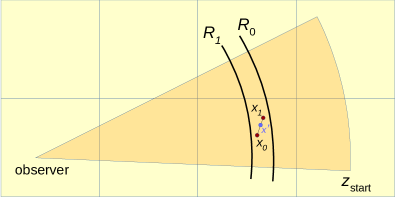
Figure 41: Geometry of the lightcone test. When a particle is drifted from comoving coordinate ${\bf x}_{0}$ to ${\bf x}_{1}$ over a time step from scale factor $a_{0}$ to $a_{1}$, GADGET-4 checks whether it is overrun by the backwards lightcone of a fiducial observer. Here $R_{0}$ is the comoving distance to redshift $z_{0}=1/a_{0}-1$, and $R_{1}$ to redshift $z_{1}=1/a_{1}-1$. If an intersection with the lightcone occurs, an interpolated coordinate ${\bf x}^{\prime}$ corresponding to the crossing time is registered in the lightcone output. The simulation box (yellow squares) may need to be periodically replicated to cover the full comoving volume of the lightcone, as sketched here. The code allows for multiple lightcones that may have a variety of angular geometries (full sky, octants, pencil beams, etc.), and variable redshift depth.

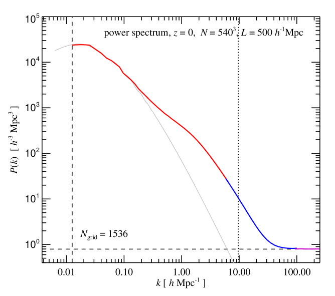
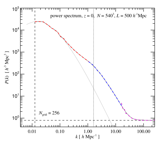
Figure 42: Example for a dark matter power spectrum measurement with the inlined routines in GADGET-4, which employ the folding technique to go significantly beyond the Nyquist frequency of a single mesh. The top panel shows a measurement with an already quite large $1536^{3}$ base grid (red lines), augmented with two further measurements with different folding factors to obtain results at progressively higher $k$ (blue and magenta lines). Even though the underlying simulation has only $512^{3}$ particles, a single $1536^{3}$ measurement would have at most reached the Nyquist frequency of that mesh (dotted line), and hence would be insufficient to measure the power on the smallest resolved scales and down to the shot noise limit (horizontal dashed line). The vertical dashed line on the left indicates the fundamental mode of the box, and the thin grey line is the linear theory power spectrum. In the bottom panel, the measurement is repeated, but this time using only a Fourier grid with $256^{3}$ cells (coloured dashed lines). Without the folding technique, the dynamic range of the measurement would be seriously limited. Using it, however, the same result as for the $1536^{3}$ mesh (which is repeated with a thin solid line in the background) is recovered in a computationally cheap way.

Whenever a particle is drifted in position space (which happens exactly in one place in the code), it is subjected to a lightcone test. Suppose the particle is moved from comoving coordinates ${\bf x}_{0}$ to ${\bf x}_{1}$ over the course of a timestep interval going from scale factor $a_{0}$ to $a_{1}>a_{0}$. Corresponding to these times are comoving distances $R_{0}$ and $R_{1}<R_{0}$ of the outer edge of the backwards lightcone (which reaches the observer at the present). If the observer is located at coordinate ${\bf q}$, then the comoving distance vectors to the observer are given by

$${\bf d}_{0/1}={\bf x}_{0/1}-{\bf q}+{\bf n}\,L,$$ (115)

where ${\bf n}$ is an (arbitrary) integer triplet accounting for periodic replicas of the simulation box. The particle can be placed onto the lightcone output during this step if and only if

$$R_{0}>|{\bf d}_{0}|\;\;\;\mbox{and}\;\;\;R_{1}<|{\bf d}_{1}|.$$ (116)

This condition can in principle be fulfilled multiple times for different ${\bf n}$, hence it is important to test for all possibilities arising from translations of the particle box. The maximum extension $z_{\rm max}$ can help here to reduce the comoving volume covered by the lightcone. If one detects in this way that the particle is overrun by the backwards lightcone, we determine the comoving coordinate and time (i.e. scale factor) where precisely this happens through linear interpolation (${\bf x}^{\prime}$ in the sketch). The resulting interpolated particle phase-space coordinates are then written into a temporary buffer.

Whenever a full timestep is completed, we check whether the temporary buffer is filled by more than some nominal number of particles, in which case the lightcone data is dumped and the buffer is cleared. The same also happens when the simulation finishes, at which point the remaining lightcone data still in the buffer is flushed in a lightcone dump. If such a lightcone dump occurs, the particle coordinates are tested against the angular mask of one or several lightcones that have been defined, and against their redshift boundaries $z_{\rm start}$ and $z_{\rm end}$. Only if a particle matches this selection, it is really written to a particle lightcone file, if appropriate also to several of them. Like all other outputs of the code, the I/O itself can be done in parallel (spread across multiple files), and uses HDF5 as preferred file format.

Our lightcone code and the built-in group finders also support the possibility to determine halos directly on the lightcone, using the lightcone particles themselves. With this option, one can forego outputting the particles on the lightcone, but rather do this for halos only, in order to substantially save on storage volume. This nevertheless allows later applications such as HOD mocks or gravitational lensing that are free of any discontinuities or ambiguities in the lightcone construction, which typically occur in schemes that instead patch together a set of time-slices (Hilbert et al., 2007).

To avoid edge effects, the temporary lightcone buffer internally always uses an all-sky geometry, even if only narrower particle-lightcones or halo-lightcones are constructed. Whenever lightcone data is flushed to disk and groups on the lightcone are desired, GADGET-4 first runs a FOF group finder directly on the temporary particle lightcone data, followed optionally by a run of SUBFIND. The actual code that is executed is the same that is also used for the ordinary group finding (these are templated C++ routines that are simply applied to a different particle data structure), such that the same set of group and subhalo properties are automatically computed in a consistent way. This also carries over to the output itself, i.e. if particle data for the lightcone is produced (and not only halos on the lightcone are output), the particle data on the lightcone is stored in group order, allowing one to easily and selectively retrieve the lightcone particles making up a given substructure, just like for ordinary timeslices. We note that the code also takes care that groups are not split up by subsequent dumps of lightcone particle data. This is accomplished by computing for each identified group a nearest distance to the fiducial observer. If this is not further away than the inner boundary of the current dump plus the linking length, the group may not yet be complete. It is then ignored in the present lightcone dump, and all of its particles are kept in the temporary buffer such that the group will be reassessed in the next lightcone dump after having had a chance to grow further.

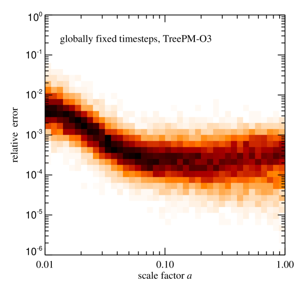
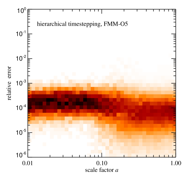
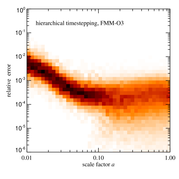
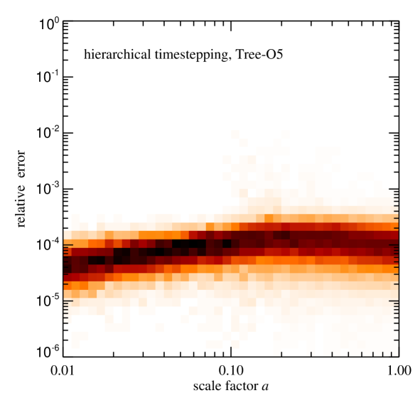
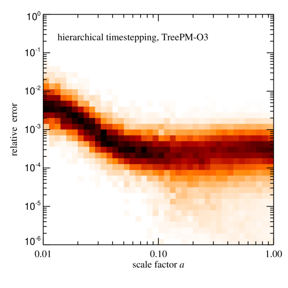
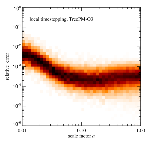
Figure 43: Force error distributions as a function of scale factor during cosmological simulations with $256^{3}$ particles and a starting redshift of $z=99$. The different panels show on-the-fly measurements during GADGET-4 runs with different force calculation algorithms and different timestepping schemes, as labelled. The force accuracy is assessed by selecting small random subsets of particles after every force computation, followed by computing the force for them by direct summation. Doing this over the course of a full simulation can reveal temporal variations of the force accuracy due to the evolving clustering state, and by inlining the measurements in this way into the actual timestepping procedure, the semantics of the code also for partially occupied timebins is explicitly tested.

Finally, a further feature of GADGET-4 is the possibility to produce particle lightcones composed only of those particles that have at some point been a most-bound particle at a previous group/subhalo catalogue. This is useful to construct mock galaxy light-cones based on physical galaxy formation models computed with semi-analytical models. For example, in semi-analytic codes like L-GALAXIES, these particles mark the locations of semi-analytic galaxies that do not have an associated dark matter subhalo any more, but are instead ‘orphaned’ and now tracked by a formerly most-bound particle of a subhalo that has dropped below the mass threshold for tracking due to tidal truncation.

In practice, the idea of this is to compute group catalogues for (many) time-slices on-the-fly, which are used to compute detailed merger trees. They are also used to mark those particle IDs that have at some point been a most-bound particle in one of those groups, and only those particles are output to particle lightcones. In a postprocessing step, the semi-analytic code then evolves a galaxy population along the merger trees. At any given time, this population features a unique most-bound particle ID for every galaxy. It thus becomes a task of matching these IDs to those appearing on the lightcone at the particular lookback time stored for the lightcone particle to obtain a high quality mock galaxy catalogue. We note that this procedure in principle does not require the creation of any particle dumps on disk at all, which we argue is a great simplification and may even be a prerequisite to create extremely large mock catalogues in this way. Note also that the use of semi-analytic models is preferable on physical grounds to HOD, SHAM, or random sampling from SAM merger trees that only take the halo mass into account, because it allows effects such as assembly bias to be properly taken into account (see for example Hadzhiyska et al., 2020, for an analysis of HOD limitations).

7.6 Power spectrum estimation

The PM gravity solver of GADGET-4 provides the basis to a built-in measurement routine for the matter power spectrum. To vastly extend the dynamic range to scales below the nominal grid scale of the employed grid, we employ the ‘self-folding’ trick described in Jenkins et al. (1998), allowing to reach down to the gravitational softening lengths or even below, if desired. This amounts to measuring several power spectra over different frequency ranges, one is for the normal periodic box of size $L$ that is covered by the PM-grid of dimension $N_{\rm grid}$. Further spectra are computed by folding the box onto a power-of-two integer subdivision of itself, i.e. effectively the simulation box is stacked on itself by imposing a smaller periodicity scale, for example $L/16$. This means that only every 16-th mode in $k$-space is measured when the power spectrum is determined from this folded density field. But this downsampling is irrelevant for the high-$k$ regime we are interested in with this measurement. In fact, by using the full box on large scales and the folded box (or boxes) on small scales, a continuous and accurate power spectrum measurement over a very wide range is reached.

As discussed in Springel et al. (2018), to cover the full dynamic range of the largest cosmological simulations presently done, computing three folded spectra with folding factors of 16 represents a good practical compromise, so this is implemented in GADGET-4. In Figure 42, this is illustrated for a small cosmological box. The code supports an automatic measurement of the power spectrum whenever a snapshot is written, but one can also apply GADGET-4 to an existing snapshot for measuring the power spectrum in postprocessing. Power spectra separated by particle type (say for example dark matter and baryons) are also possible, and are computed besides the total matter power spectrum. The shot-noise is computed in each case, if needed by taking variable particle masses into account.

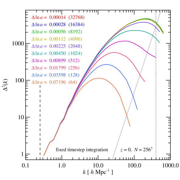
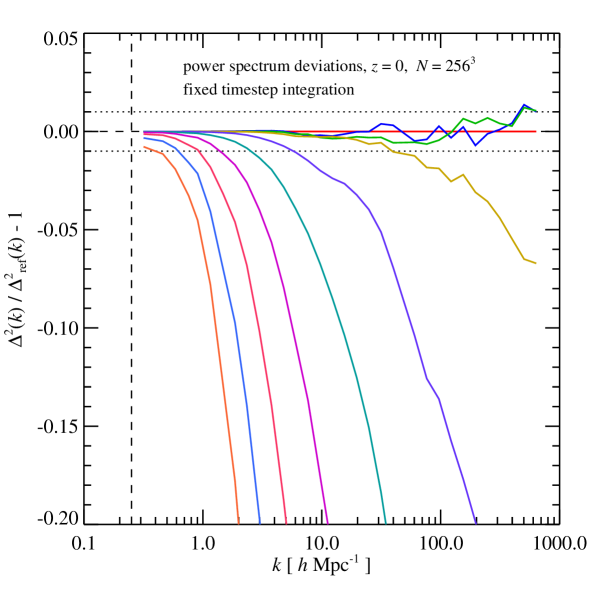
Figure 44: Non-linear power spectra obtained at $z=0$ for a cosmological simulation when different fixed timestep sizes $\Delta\ln a$ (left panel, as labelled) are used. The simulations followed $256^{3}$ particles in a periodic box of $L=25\,h^{-1}{\rm Mpc}$, with a starting redshift of $z=99$. In all the calculations, the force accuracy was chosen conservatively, and assured to be better than a maximum relative error of order $10^{-3}$. Spatial randomization after every step has been used, too, i.e. the results should be to good approximation unaffected by force errors, and thus only test the time integration accuracy. The inclined grey line in the panel on the left shows the shot noise limit, which has been subtracted from the measurements. The dashed vertical line indicates the fundamental mode of the boxsize, and the numbers in parentheses after the timestep sizes give the total number of time steps taken by the corresponding simulation. The panel on the right hand side shows the deviations of the power spectra at $z=0$ relative to the simulation with the smallest timestep, which we identify as a fiducial simulation that is fully converged in terms of timestepping accuracy. We see that timesteps that are 2 or 4 times larger than used for this run give essentially indistinguishable results; the maximum difference of their power spectra stays within 1% (dotted horizontal lines), and no systematic trend in these deviations is apparent. This is different for the simulation with an 8 times larger stepsize (i.e. the run with only 4096 steps in total). Its power on the smallest scales starts to show a systematic deficit of up to $\sim 5\%$ for the highest resolved $k$. For still larger timesteps, this deficit rapidly becomes very large in the non-linear regime, rendering these simulations hopelessly inaccurate. Interestingly, modes that stay in the linear regime (for this box-size this is basically only the fundamental mode) are reasonably well followed even for just 64 steps.

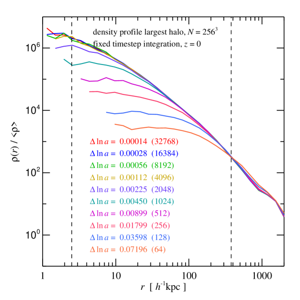
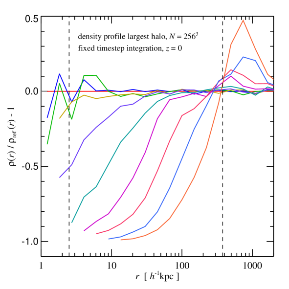
Figure 45: Spherically averaged density profile of the largest halo in simulations integrated with different fixed timesteps $\Delta\ln a$ (the same runs are shown in Fig. 44), evolved from a starting redshift of $z=99$ to $z=0$. These simulations have been run with high force accuracy so that they are only affected by errors from the time integration. The vertical dashed lines mark the softening length and the virial radius (enclosing 200 times the critical density) of the target halo, respectively. The left panel shows the plain density profiles, whereas the right panel gives deviations with respect to the result obtained with the highest time integration accuracy. We again see that that the runs with $\Delta\ln a=0.0028$ and $\Delta\ln a=0.0056$ are still converged, whereas $\Delta\ln a=0.00112$ begins to show a central density suppression. Worse time integration manifests itself in reduced central halo densities, as expected.

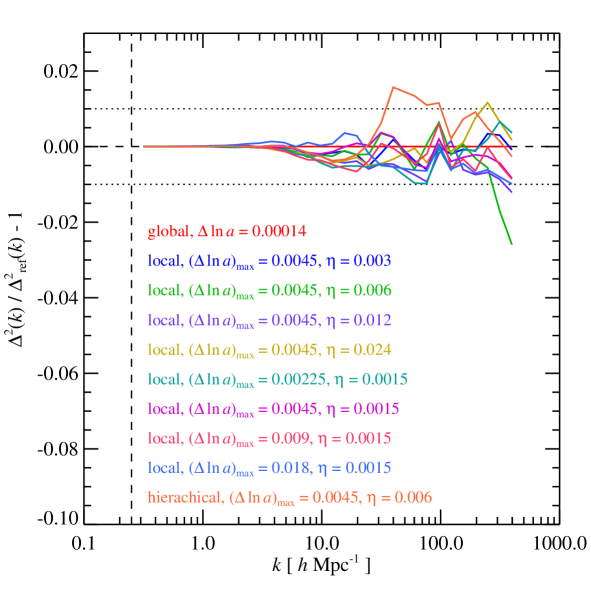
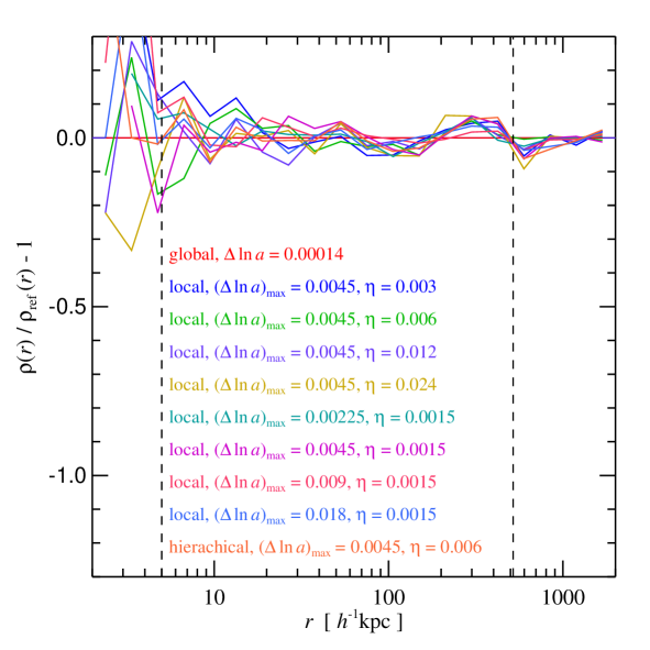
Figure 46: Relative difference of matter power spectrum (left panel) and the density profile of the largest halo (right panel) of simulations carried out with different local timestepping settings when compared to a run done with a very small global timestep. The simulation specifications are the same as for the runs considered in Fig. 45, and we in fact use the run with a fixed $\Delta\ln a=0.0014$ from that series as our fiducial ‘ground truth’ result here. The local timestepping schemes are specified by a parameter $\eta$ controlling the timestep sizes of individual particles, plus an additional maximum allowed timestep size $(\Delta\ln a)_{\rm max}$. We consider 8 different choices for these settings, and also include one realization of the hierarchical time integration scheme. Within the noise, all runs give results of acceptable accuracy, without evidence for clear systematic deviations, suggesting a reassuring robustness of these time integration schemes.

7.7 Cosmological initial conditions creation

Another feature we integrated into GADGET-4 is the ability to create cosmological initial conditions, a functionality we previously provided in the stand-alone N-GENIC code. In particular, it is now possible to create the initial conditions at start-up of a simulation run, avoiding the need to create them first in a separate step. This also avoids the need to store them on disk (although this can be done, if desired). It is also possible to create initial conditions in stretched cuboids, not only in cubic periodic boxes.

Technically, the code uses either the Zel’dovich approximation or second-order Lagrangian perturbation theory (Scoccimarro, 1998; Scoccimarro et al., 2012), and sets up a realization of the power spectrum in Fourier space. It thus implements similar functionality as the 2LPTIC code originally based on N-GENIC. Both Cartesian grids and glass distributions (White, 1996) for the initial particle load are supported. For the latter, one can also opt to enable a deconvolution filter that accounts for the smoothing effect of interpolating the displacement field from a grid to the irregular particle distributions. By default, a given initial conditions seed ties down the density field for a given box everywhere, i.e. if the simulation resolution is increased later on, the large-scale phases are retained and one gets the same large objets and cosmic web as before. Note that the maximum size of Fourier meshes that can be realized in practice limits the dynamic range of this approach for zoom simulations. It would thus be worthwhile to integrate the much more sophisticated PANPHASIA approach (Jenkins, 2013) for defining the phases in real-space in the future. The initial conditions creation is fully parallel and able to create essentially arbitrarily large initial conditions, either with dark matter only, or with dark matter and gas. If desired, the variance suppression technique by Angulo & Pontzen (2016) can also be enabled.

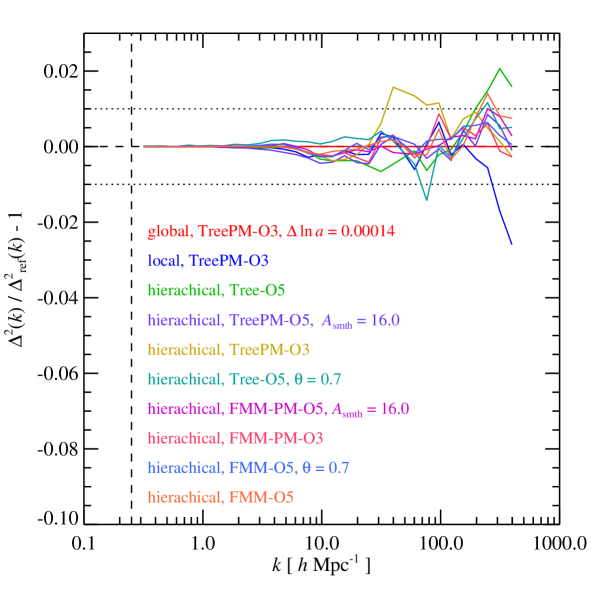
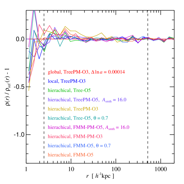
Figure 47: Similar to Fig. 46, we here consider differences in the matter power spectrum (left panel) and the density profile of the biggest halo (right panel) when run with different code settings, but we now examine variations induced by the use of different force calculation schemes. The results are evaluated relative to a run done with small global timesteps and high force accuracy, as before. All other runs are variations therefore carried out with different force calculation schemes, as labelled, and have either used local or hierarchical timestepping with $\eta=0.006$ and a maximum timestep of $(\Delta\ln a)_{\rm max}=0.0045$. Again, we find the results to be robust under these changes.

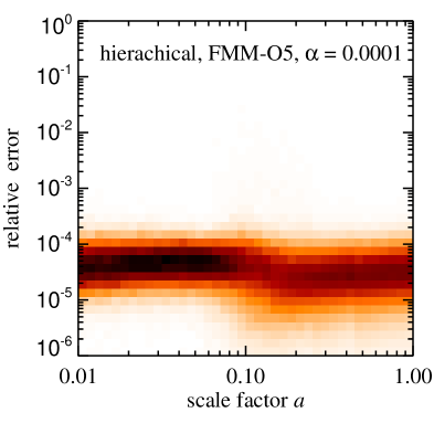
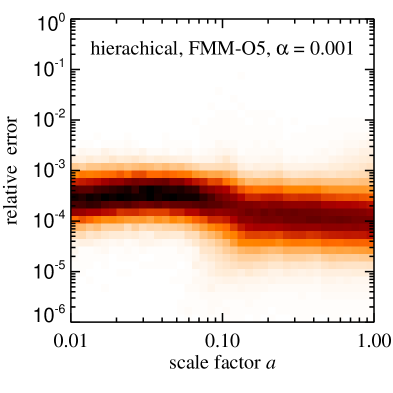
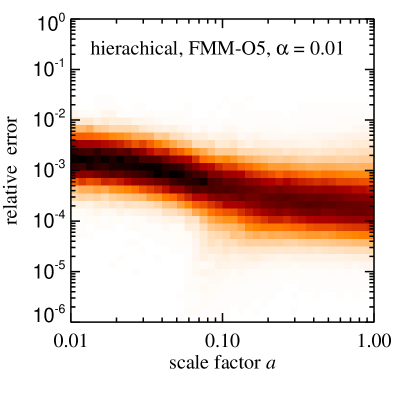
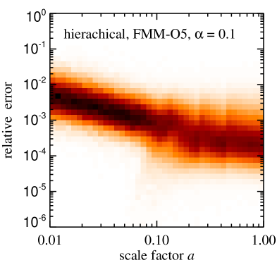
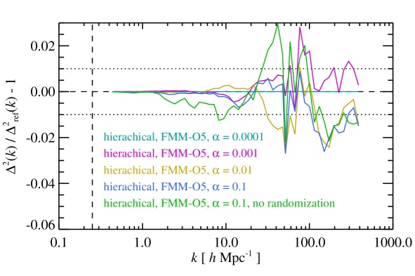
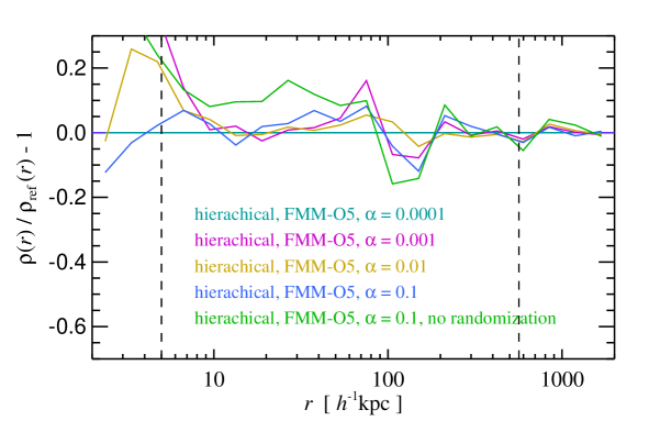
Figure 48: Sensitivity of the results of a cosmological simulation with $256^{3}$ particles to force accuracy. We here consider simulations carried out with the FMM-O5 scheme and hierarchical time integration. Our fiducial reference run uses very high force accuracy with $\alpha=0.0001$, and we then systematically degrade the force accuracy in several steps with values of $\alpha=0.001$, $\alpha=0.01$, and $\alpha=0.1$. Random translations are applied after every step with a new domain decomposition to reduce temporal correlations of force errors, except for a second run with $\alpha=0.1$ where no shifts of the particle distribution are applied, as labelled. The top panels give the force accuracy as a function of scale factor for the the four settings of $\alpha$, measured on-the-fly by comparing to direct summation forces for random sub-sets of particles that are newly drawn every step. Here the two runs with $\alpha=0.1$ with and without randomization are indistinguishable. The bottom left panel compares the power spectrum of the four lower accuracy runs with the highest accuracy run in the series, while the bottom right panel carries out this comparison for the density profile of the most massive halo in the box. The residual differences among the simulations are consistent with expectations from Poisson particle noise, except for the run with $\alpha=0.1$ without randomizations, which shows significant systematic differences with respect to the highest force accuracy run. This confirms that unbiased and random force errors are ultimately less important for collisionless dynamics than time integration errors, and that random shifts of the particle set are helpful in establishing sufficiently random distributions of the residual force errors.

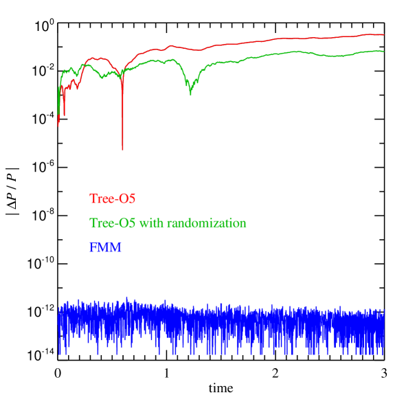
Figure 49: Total momentum error in FFM and tree-based calculations of a galaxy merger simulation. All three simulations use the hierarchical time integration scheme with local timesteps, and an expansion order $p=5$. Despite one-sided momentum updates being avoided in this case, the tree-based calculation still shows a secular drift of the total momentum of the system, due to residual small force errors that do not all add up to zero. Note that the total momentum of the system is very small here (the system is meant to be at rest), so measuring its relative error provides a particularly sensitive test. If random translations of the particle set relative to the root node are carried out after every step, the size of the error found for the Tree-based calculation is substantially reduced, but it remains present at a reduced level. In contrast, with FMM, the error vanishes entirely and the total momentum is preserved to machine precision even in the presence of local timestepping, as expected.

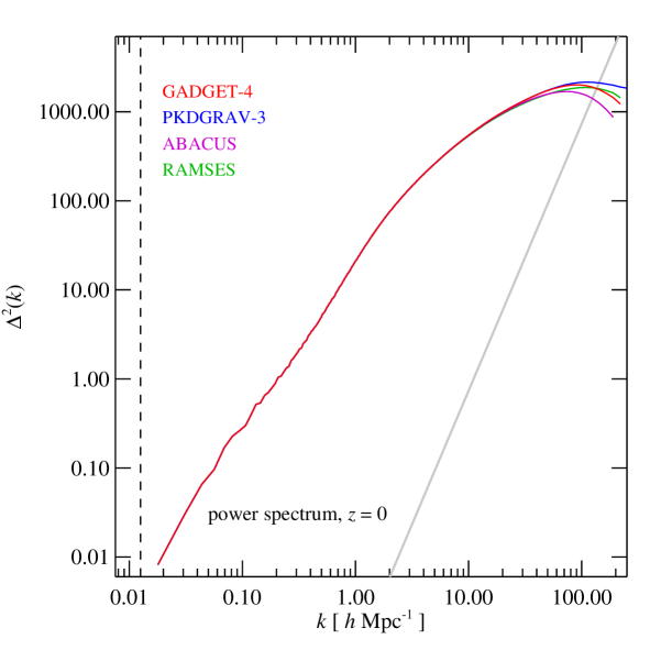
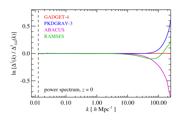
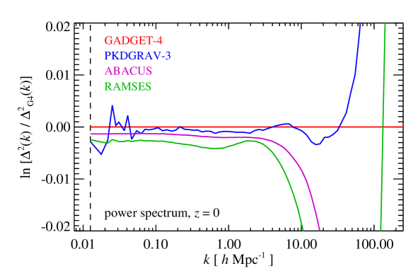
Figure 50: Power spectrum of the ‘Euclid test simulation’ discussed by Schneider et al. (2016). We compare our measurement for GADGET-4 to the results reported for PKDGRAV-3 and RAMSES in that paper, and we also include a recent recalculation by Garrison, Eisenstein & Pinto (2019) with their code ABACUS. All power spectra have been remeasured by us in identical ways from the $z=0$ particle data of the different runs. The top panel shows the power spectra of the different runs with the shot noise subtracted, the bottom two panels give the fractional differences with respect to the GADGET-4 result, with the vertical axis range adjusted to focus on small-scales (middle panel) and large-scales (bottom), respectively.

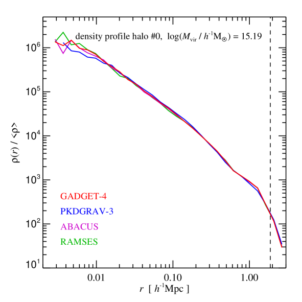
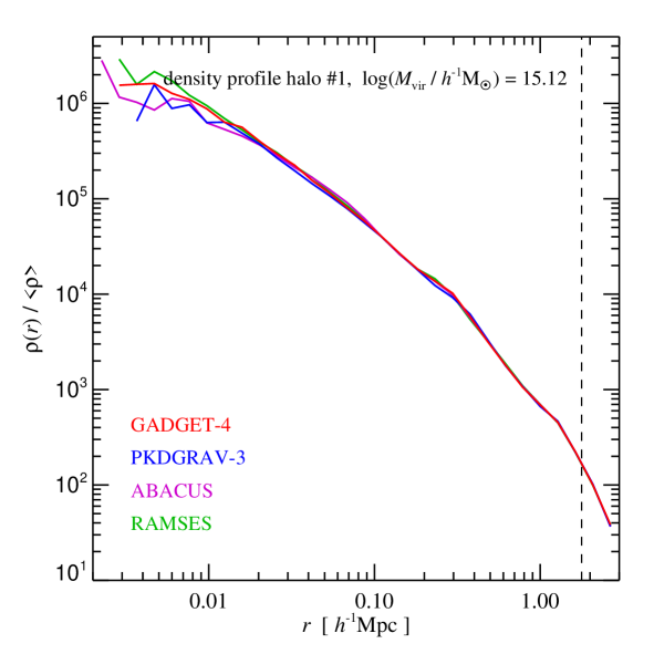
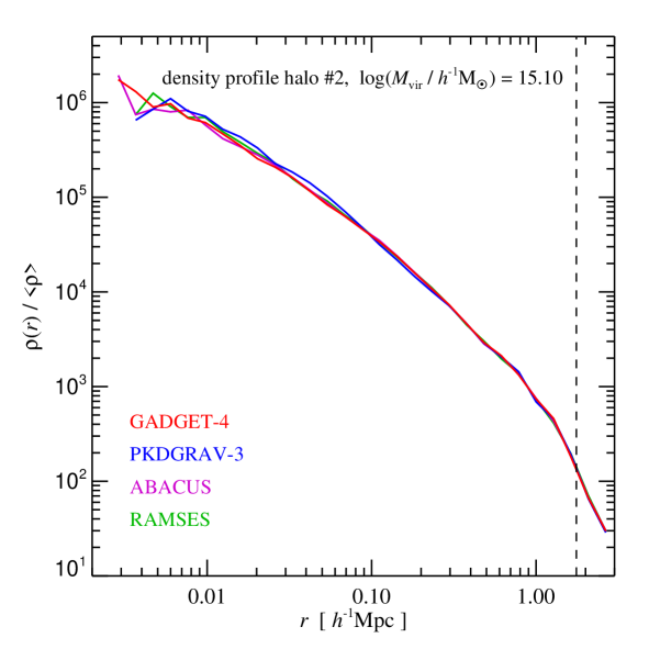
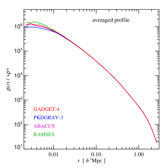
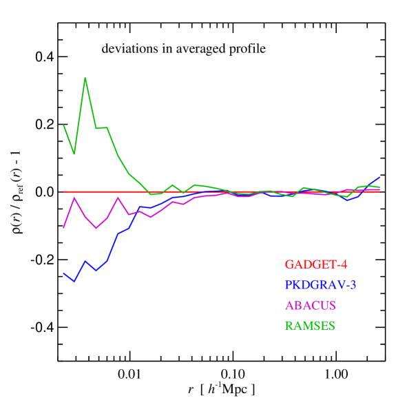
Figure 51: Comparison of halo density profiles for the ‘Euclid test simulation’ (Schneider et al., 2016; Garrison, Eisenstein & Pinto, 2019), using different cosmological codes. We have computed FOF group catalogues for the $z=0$ particle data of simulations carried out with the GADGET-4, PKDGRAV-3, RAMSES, and ABACUS codes. Group centres were determined as the potential minima of the groups in all cases, and the profiles were binned in equal logarithmic shells. The top row panels show the density profiles for the three halos with the largest virial mass (defined here as the mass enclosing a mean overdensity 200 times the critical density). The dashed vertical lines indicate their corresponding virial radii. In the bottom top left panel, we show the averaged profile for the 25 most massive halos to highlight the systematic differences between the codes. The deviations of the mean profiles relative to the GADGET-4 result are shown in the bottom right panel. By matching halo centers, we made sure that the same halos are analysed in the four simulations in all cases. For simplicity, only particles contained in the FOF halos were included in the binning; if all particles would be included, the fall-off around and outside the virial radii would be slightly less steep.

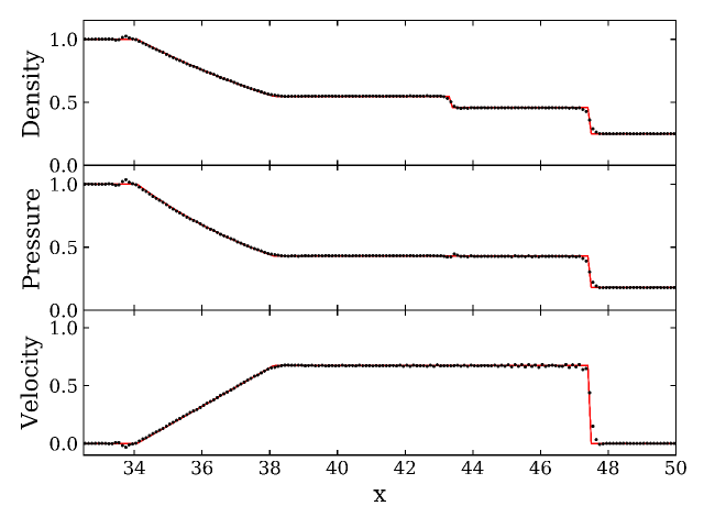
Figure 52: Shock tube test at time $t=5$ with the Wendland C6 kernel, a time-dependent artificial viscosity and density-based SPH. The resolution is given by initially $N=1440$ particles in the $x$-direction (with $L_{x}=80$). For visual clarity, we only show the average values in $x$-bins of size $\Delta x=0.1$.

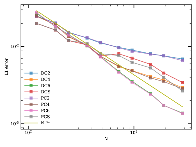
Figure 53: Convergence rate of the Sod shock tube test problem illustrated in Fig. 52. The L1 error gives the difference to the analytic solution at time $t=5$ as a function of resolution for different combinations of kernels and SPH flavours. Here $N$ is the initial number of particles in the $x$-direction. All simulations were run with time-dependent viscosity, but the results for a fixed viscosity are very similar. We find a convergence rate $L1\propto N^{-0.9}$ for the Wendland C6 kernel, which is close to the optimal value of $L1\propto N^{-1}$ (Springel, 2010b) excepted for this problem. The other kernels, especially the standard cubic spline kernel, show a poorer convergence rate due to their higher residual particle noise. The naming convention of the different results is as follow. The first character gives the flavour of SPH (D for density- and P for pressure-based), and the two other characters define the used kernel (CS stands for cubic spline, while C2, C4 and C6 refer to the Wendland kernels of different order).

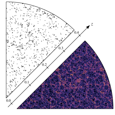
Figure 54: Example for lightcone output that can be produced by GADGET-4. We show here a 45 degrees wedge-like region of constant comoving thickness of $5\,h^{-1}{\rm Mpc}$ excised from the full lightcone. The dark matter density is projected onto the plane and shown in color-scale, with comoving distance used as radial coordinate. The axis gives the corresponding look-back redshift, which at these low redshifts is still linearly related to comoving distance to good accuracy. The wedge in the upper left shows the same region, but this time small circles are drawn to indicate halos identified by the group finder of GADGET-4, which was applied on-the-fly directly to the particles on the lightcone data. For visual clarity, only halos with virial mass above $10^{13}\,h^{-1}{\rm M}_{\odot}$ are shown, and drawn with circles that have a radius four times the actual virial radius. The base simulation of this example used a box size of $500\,h^{-1}{\rm Mpc}$ on a side with $1080^{3}$ particles, so the code replicated the box automatically a few times in each dimension to cover the lightcone (the comoving distance out to $z=0.4$ is about $1083\,h^{-1}{\rm Mpc}$), a fact that is recognizable by the repetition of structures (albeit at different evolutionary state) in the image in the horizontal direction.

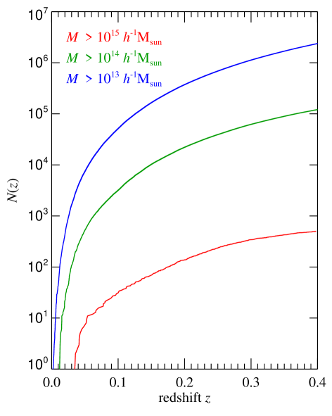
Figure 55: Cumulative mass function of halos on the all-sky backwards lightcone of a $L=500\,h^{-1}{\rm Mpc}$ test simulation (the one shown in Fig. 54), for different mass thresholds (as labelled), as a function of the lookback redshift. This corresponds to the number of objects larger than the given mass that are in principle observable out to a certain redshift. Note that the absolute counts for rich clusters are expected to be biased low in this example, due to missing large-scale power in the intermediate-size box that was simulated here.

7.8 I/O organization

The recommended default format of all output in GADGET-4 is HDF5, but the code continues to support the legacy binary formats of GADGET (called ‘format 1’ and ‘format 2’) as well. For parallel I/O, and to limit the sizes of individual files (useful for easier transfer and archival), the output can be distributed over multiple files that are written or read simultaneously. If multiple files are written in parallel, the number of simultaneous writes can be limited to avoid overburdening a filesystem. The I/O operations are scheduled automatically such that as many distinct compute nodes as possible are active at any given time within the imposed bounds, which can help to maximize the achievable I/O bandwidth on a given system.

All HDF5 output files contain a record of the configuration options and the parameterfile that was used to run the code, as well as a git hash key encoding the code version that was used to produce the data. All output fields are annotated with their units and auxiliary scaling factors needed to convert to physical values. Output data may be stored in single precision (or even in half-precision for velocities) to save disk storage space. Upon input, the code automatically detects the floating point type of the data and converts it as needed to the internal representation (this also works for the two legacy binary formats of GADGET, not only for HDF5). Another useful feature is that GADGET-4’s I/O routines support on-the-fly lossless compression of output fields, which is fully transparent to analysis scripts thanks to the HDF5 library. The achievable compression ratios can be quite high for some of the fields, in particular for integer data related to merger tree bookkeeping, or for the ID field used to tag simulation particles.

8 Code validation and convergence tests

We now want to discuss the question which code settings are in practice required to reach converged answers for the non-linear mass distribution, and whether this can be achieved robustly for all the many combinations of gravity solvers and time-stepping approaches supported by GADGET-4. For a semantically correct code, stable results that are invariant under small changes of the integration parameters should be obtained if there are negligible force errors and negligible errors due to the time integration. In the absence of hideous bugs in the code, this limit should be reached for sufficiently small settings of the force accuracy parameters and of the timestep sizes. But note that requesting recovery of identical individual phase space positions of particles makes no sense in practice even in this limit, because individual particle orbits tend to be chaotic in the non-linear regime (e.g. Thiébaut et al., 2008; Keller et al., 2019; Genel et al., 2019) and are merely Monte Carlo tracers of the underlying collisionless fluid. Rather, statistical quantities that depend on a collection of particles, such as halo density profiles, the halo mass function, or the matter power spectrum are of interest here, and can be expected to converge to a unique answer for high force accuracy and sufficiently accurate time-stepping, modulo sampling noise present due to the finite number of particles or modes used.

It depends on the particular quantity under study at what point a simulation model is giving a converged answer (for example, getting the total mass of a halo right is easier than getting its central density profile right). For definiteness, we in the following pick the matter power spectrum, and the inner regions of halos for our convergence experiments. For our test simulations, we typically consider the relative deviations to a fiducial “fully converged” simulation, which we in practice identify with the simulation with our most conservative integration settings. In the absence of analytic solutions, this provides a heuristic approach to test whether the simulation outcomes are robust to variations of the integration settings.

8.1 Validating the time integration schemes

We begin by aiming to establish that under conditions of negligible force errors, integrations carried out either with a global timestep, with standard local timesteps, or with the hierarchical timestepping introduced here, all give the same results provided sufficiently conservative timestep sizes are chosen.

To this end, we carry out simulations with conservatively high force accuracy settings and explicitly verify during the simulation run that forces in all parts of the algorithms have a high relative accuracy. This is done by randomly picking a small subset of particles in every step, and computing a direct summation force for them for comparison. A result of this test is illustrated in Figure 43, where we look at the force error distributions as a function of time in a cosmological simulation with $256^{3}$ particle in a $25\,h^{-1}{\rm Mpc}$ box, for a variety of typical setups. We show six examples of runs carried out with different force calculation algorithms (using Tree and FMM schemes of different order, and optionally accelerated with the TreePM or FMM-PM schemes), and different timestepping approaches. As we saw also earlier, it is more challenging to obtain low relative force errors at high redshift for the tree-based algorithms, especially for moderate expansion order. This is primarily due to the small absolute sizes of the peculiar accelerations there. However, all algorithms can be pushed to relative force errors well below $10^{-2}$ even there. Importantly, there are no outliers towards much large force errors, serving as an important “in-situ” validation of the implementation of the parallel force computation algorithms. Combined with our scheme for decorrelating force errors in time through random translations, we expect these force errors to be small enough to affect the following results only at negligible levels, something that we also verified with additional tests to be discussed later on with still lower residual force errors.

Next, we turn to the time integration schemes, with a view to establish how small the steps at least need to be to obtain converged results. We first consider simulations with fixed global timesteps, in order to see the general impact of time-stepping accuracy on collective results. We begin with deliberately coarse stepping, and then subsequently improve it by factors of two. In Figure 44, we compare the power spectra of the resulting sequence of simulations and their deviations from the run with the shortest timestep, which we identify with the most accurate result in this series. These test simulations again use $256^{3}$ particles in a relatively small box of $25\,h^{-1}{\rm Mpc}$ in order to still have a relatively high mass resolution and a high degree of non-linearity comparable to current high-resolution simulations done for large-scale structure studies. We see that for a fixed timestep size of $\Delta\ln(a)=5.6\times 10^{-4}$ or lower, the power spectrum is converged to better than $1\%$ accuracy all the way to scales corresponding to the softening length. This corresponds to at least 8192 steps from redshift $z=99$ to $z=0$. For the fundamental mode, which is starting to leave the linear regime for this small box size, a step size as low as $\Delta\ln(a)=7.2\times 10^{-2}$ can already be sufficient (corresponding to just 64 steps) to limit deviations from a converged answer to less than $1\%$, but this is inadequate already for the mildly non-linear regime, and hopelessly inaccurate for the highly non-linear regime.

In Figure 45, we extend this comparison the spherically averaged density profile of the largest halo found in the simulation box. Consistent with the power spectrum findings, here the $\Delta\ln(a)\leq 5.6\times 10^{-4}$ setting provides a density profile that is indistinguishable within the noise from runs that use considerably finer timestepping, whereas twice as large steps show already small but systematic reductions of the density around $r\sim 10\,h^{-1}{\rm kpc}$. Insufficient time integration accuracy generically shows up as a reduction in the central halo density, as expected.

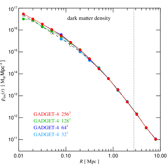
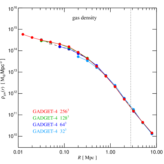
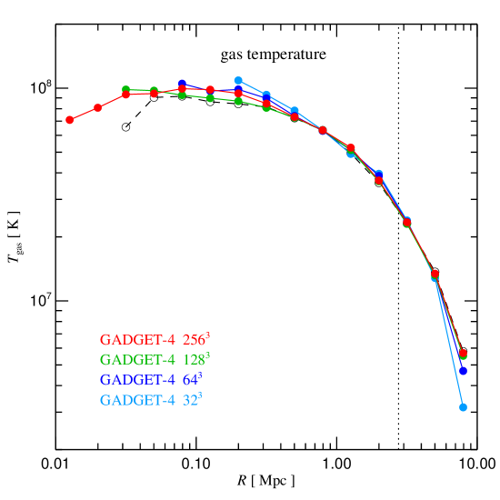
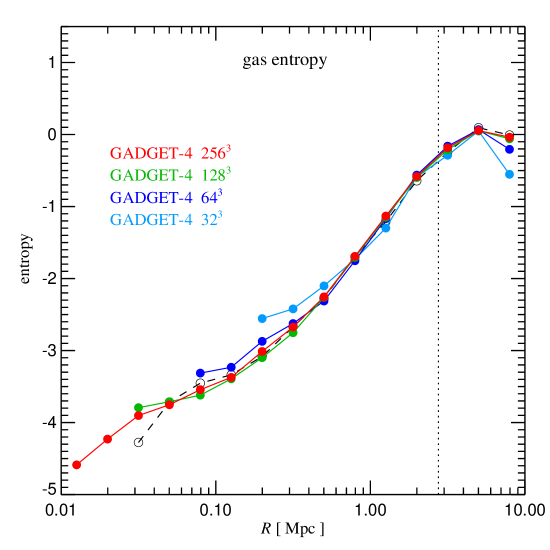
Figure 56: Dark matter density, gas density, temperature, and entropy profiles of the cluster studied in the Santa Barbara cluster comparison project (Frenk et al., 1999), here computed at the maximum $2\times 256^{3}$ resolution that was created (but not actually used) at that time. We compare the highest resolution result to runs carried out at $2\times 128^{3}$, $2\times 64^{3}$, and $2\times 32^{3}$ resolutions, and to the average of all the different simulation results reported in Frenk et al. (1999), which are shown as dashed lines. Our simulations were here computed with the pressure-based SPH version. Compared to mesh-based calculations and some alternative SPH formulations that try to explicitly account for mixing, the results show quite low entropy in the centre. The density-entropy formulation (Springel & Hernquist, 2002) tends to give still slightly lower central entropies, presumably reflecting a spurious suppression of turbulent mixing at the resolution scale.

It is now interesting to compare time integration schemes that employ local timestepping with the ‘converged’ result obtained for a globally fixed timestepping. This is considered in Figure 46, where the left panel shows relative differences in the power spectrum with respect to the fiducial “ground truth” result (global timestep with 32768 steps), and the right panel shows this comparison for the density profile of the largest halo. We consider a variety of combinations of a maximum timestep size (to give good accuracy for small modes $k$ that stay in the linear regime) with a local timestepping parameter $\eta$ that controls the accuracy within dense halos. Clearly, for this softening setting, a value of $\eta=0.006$ appears required to obtain fully consistent results, while $\eta=0.012$ is not quite as good as some systematic reduction in power of $\sim 0.5\%$ becomes visible in the range $k\simeq 10-100h\,{\rm Mpc}^{-1}$. We have also included a test with hierarchical timestepping which produces consistent results. Overall, the results provide an important confirmation that local timestepping for collisionless dynamics in structure formation is viable and a highly accurate approach to accelerate the simulations (see also Power et al., 2003). Note that even here, where the dynamic range in timescales is still fairly limited, this already entails a significant computational saving compared to the use of a global timestep.

8.2 Validating the force accuracy of different schemes

For a simulation that is converged with respect to timestepping, we can now go back and ask whether the different force calculation algorithms implemented in GADGET-4 still give the same results if larger force errors are tolerated, as is often done in practice to keep the computational cost at bay.

This is addressed in Figure 47, where we show simulations done with different force computation schemes, again compared to the fiducial “ground truth” fixed timestep run. Here, we consider a variety of different force calculation schemes possible with GADGET-4, using a set of force accuracy parameter settings, and we also include a number of modifications of the time stepping scheme at the same time, thus covering a range of code settings that may be encountered in practice.

Reassuringly, the results overall suggest that the code indeed produces consistent results for high enough force accuracy and high enough time integration settings, pretty much independent of which of the code’s force computation algorithms or time-stepping schemes is used. This degree of robustness is important, as it offers a certain degree of protection (but unfortunately no guarantee) against a poor quality of results due to the adoption of non-ideal settings.

The above also begs the question how much the force accuracy could be degraded – assuming good time integration accuracy is preserved – before significant differences in the results show up, and if they do, where they become noticeable first. This is obviously important because computing forces with very small error is computationally expensive. Aiming for something that is excessively conservative here has the potential to needlessly increase the computational cost, just like excessively small timesteps would do. The crux is of course that erring on the other side is even more problematic, because there is often little advantage in obtaining results quickly if they are of poor quality, and worse, not being aware of this could lead in extreme cases to misleading scientific conclusions. On the other hand, depending on the scientific question that is asked, there are of course sometimes situations where approximate answers are perfectly sufficient. It is hence important to be fully aware of the accuracy of the results one obtains.

To partially address this question, we show in Figure 48 results where the force accuracy is systematically reduced while the time integration accuracy is kept high. For the lowest force accuracy setting, we carry out the simulation a second time by disabling the random spatial translation of the particle set in every domain decomposition. We see that the results are rather stable, even for relatively coarse settings, provided that randomizations are applied. This confirms that small force errors that are random and uncorrelated in time, do not seriously impair collisionless dynamics. Time integration accuracy is in that sense the more important category, as errors introduced here invariably show up in the results. However, the run with a low force accuracy setting and without random translations shows clear systematic differences relative to the high force accuracy simulation, both in the matter power spectrum and the mean density profiles of the largest halos. This confirms that random shifts of the particle set are helpful in establishing sufficiently random distributions of the residual force errors.

Finally, as an aside, we check whether the total momentum is indeed conserved to machine precision when the FMM scheme and hierarchical time integration are used. In Figure 49, we consider the total linear momentum in the simulation box as a function of scale factor, comparing FMM and tree-based simulations. Furthermore, we repeat this test without the randomization approach for reducing correlated force errors. The results confirm our expectations. While FMM with hierarchical (or global) timestepping manifestly confirms momentum to machine precision, this is not the case for any variant of the normal Tree algorithm. However, translational randomization of the particle set in every step does already reduce the size the corresponding secular error can build up to.

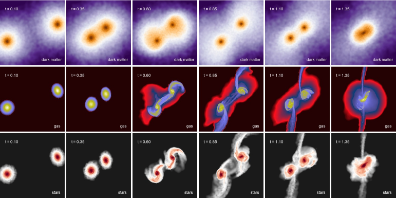
Figure 57: Visualization of a galaxy merger simulation carried out with GADGET-4. The top row illustrates the evolution of the projected dark matter density in a major merger of two equal mass disk galaxies that collide on a prograde, zero-energy orbit. The middle row shows the gas phase, which initially comprises 33% of the disk mass of the galaxy models, and is actively forming new stars. The other 66% of the initial disk mass are made up of preformed stellar material, whose evolution is illustrated in the bottom row. All panels are $160\,{\rm kpc}$ on a side, and the time of the individual images is given in Gyr in the labels.

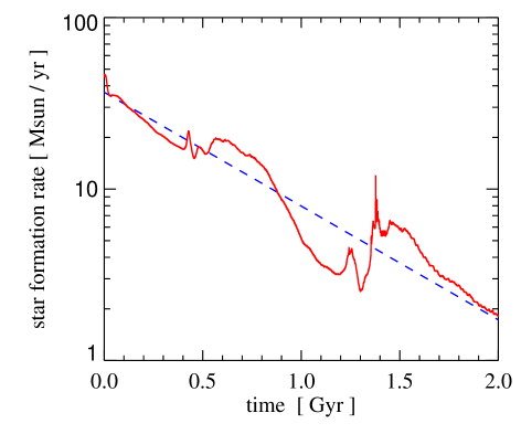
Figure 58: Evolution of the star formation rate in a galaxy merger simulation (the one illustrated in Fig. 57). The overall trend is that the gas mass is used up to make stars with a consumption timescale of around $1\,{\rm Gyr}$, as indicated by the dashed line. This is modulated by the merger, which first induces a mild enhancement around the first encounter at $t\sim 0.6,{\rm Gyr}$, followed by a reduction due to tidal removal of gas, and a mild starburst at $t\sim 1.4\,{\rm Gyr}$, when the galaxies collide a second time and then quickly coalesce.

8.3 Comparing results to other N-body codes

It is also important to compare N-body results with other codes in order to assess remaining systematic uncertainties in their predictions, especially in the non-linear regime of cosmic structure formation, where definitive analytic results are not available. The exquisite accuracy demanded by modern cosmological surveys that target dark energy, such as EUCLID, provides additional motivation for this, because here simulation results need to reach a nominal accuracy of 1 percent or better to meet the statistical needs of these surveys. It is not readily clear whether current codes agree to this precision, and whether this is reached for standard settings of numerical nuisance parameters that control timestep size, force accuracy, or softening length (Smith et al., 2014).

Schneider et al. (2016) presented in this context a comparison of the cosmological codes PKGRAV-3, RAMSES, and GADGET-3, focusing on the non-linear power spectrum in a large $2048^{3}$ simulation in a $500\,h^{-1}{\rm Mpc}$ box, the “Euclid test simulation”. While the runs showed good agreement on large scales, there were a few noticeable difference at high $k$. In particular, GADGET-3 came out a bit lower than the other two codes, whereas RAMSES was slightly higher. While overall this agreement can be deemed satisfactory, it was arguably less good on small scales than one may hope for, given that the comparison stopped already at $k\simeq 10\,h\,{\rm Mpc}^{-1}$, i.e. was only done from the fundamental node to a scale equal to the mean particle spacing. This is basically where the highly non-linear regime only begins; the softening scale is still a factor $\sim 40$ smaller than the mean particle spacing, and in principle the simulations should agree over most of this range, too.

The EUCLID test simulation of Schneider et al. (2016) has recently been revisited by Garrison, Eisenstein & Pinto (2019) using the ABACUS code, which is a novel out-of-core N-body code that uses GPU-accelerated direct summation for short-range forces, and an FMM-based convolution method with a fixed grid to compute the long-range forces. The authors emphasize that the high-force accuracy resulting from this method should yield a high fidelity result for the test run. Their simulation was however carried out with a global timestepping scheme using a comparatively coarse step size. While this proved sufficient to give good agreement with the power spectra obtained by Schneider et al. (2016) up to the mean particle spacing, according to our earlier tests on timestepping convergence, it is not clear whether the fidelity of the result can be expected to extend into the highly non-linear regime at the centres of halos.

In any case, it is interesting to also apply GADGET-4 to the corresponding initial conditions of Schneider et al. (2016) and see what we get. We show our results in Figure 50, where the top panel gives the shot-noise subtracted power spectrum, this time measured accurately to much smaller scales than considered in Schneider et al. (2016) and Garrison, Eisenstein & Pinto (2019). The relative differences in the power spectrum are given in the two bottom panels. We include here the original simulation particle data from Schneider et al. (2016) and Garrison, Eisenstein & Pinto (2019), but use our own power spectrum routines for consistency in the measurements.

Interestingly, while the simulations agree again reasonably well over the range $k<10\,h\,{\rm Mpc}^{-1}$, the differences in the highly non-linear regime quickly become very large. GADGET-4 agrees best with PKDGRAV out to about $k\sim 40\,h\,{\rm Mpc}^{-1}$, but then PKDGRAV gives considerably higher small-scale power. In contrast, RAMSES and especially ABACUS show a deficit of power on nonlinear scales, which in the case of RAMSES is however rather a dip relative to GADGET-4 that eventually turns around and becomes an excess at the smallest scales. The systematically low power of ABACUS on very small scales may well reflect the more limited time-integration accuracy of the corresponding run due to use of global timestepping, as suggested by the findings discussed earlier in this section. The differences of GADGET-4 with respect to RAMSES and PKDGRAV on very small scales could instead be explained by different force softening laws. Another interesting effect is that some $k$-modes at the largest scales show small fluctuating differences in growth in PKDGRAV, and to a lesser degree in ABACUS, relative to RAMSES and GADGET-4. This probably reflects the lower accuracy of a pure real-space evaluation of the large-scale gravitational field compared to a spectral methods. We remark that we have also repeated a run with GADGET-3. Curiously, this shows a result very close to GADGET-4, and hence gives slightly higher small-scale power than the run reported in Schneider et al. (2016). This was also independently found by Angulo et al. using the L-GADGET-3 variant of GADGET. The original result reported in Schneider et al. (2016) for GADGET-3 thus seems to be slightly anomalous, for a still unidentified reason, but a slightly high softening setting or a poor timestepping accuracy setting could be a possible explanation.

In Figure 51, we extend this comparison to the density profiles of the largest halos in the box. In the top three panels we consider in an exemplary fashion the density profiles of the largest three halos, while in the bottom panels we examine the averaged profile of the 25 most massive halos (bottom left). The systematic differences in the mean profile predicted by the codes are shown in the lower right panel. We made sure that really the same halos are identified in this comparison in all cases. While the profiles agree quite well down to a scale of $\sim 30\,h^{-1}{\rm kpc}$, there are noticeable systematic differences in the innermost regions of the halos. With respect to the GADGET-4 result, RAMSES finds higher dark matter density by up to $30\%$ at around the softening scale, while the opposite is the case for ABACUS and PKDGRAV. Part of this is likely driven by different effective softening laws and time-stepping accuracy, but it will be interesting to identify and eliminate the root cause of these relatively small but systematic code differences in the future.

8.4 Convergence in a basic SPH shock tube problem

Finally, we test our different SPH implementations presented in Section 5 by comparing their convergence rate in an often used standard Sod shock-tube problem (Springel, 2005, 2010a; Hu et al., 2014; Hopkins, 2015). We consider a two-dimensional stretched periodic box with sizes $L_{x}=80$ and $L_{y}=10$, filled with an ideal gas initially at rest with adiabatic index $\gamma=1.4$. The half-space for $x<40$ is filled with gas of unit density and unit pressure ($\rho_{1}=1$, $P_{1}=1$) while the half space for $x>40$ is filled with low-density ($\rho_{2}=0.25$) and low-pressure ($P_{2}=0.1795$) gas. We let the system evolve until time $t=5$, which is enough time to stretch the self-similar wave structure over a significant spatial range while avoiding overlap with the waves generated from the equivalent problem at the periodic box boundaries. To easily create initial conditions with different resolutions, we use Cartesian grids for the initial particle distribution in both half-spaces.

In Figure 52 we illustrate the result obtained for the Wendland C6 kernel with time-dependent viscosity and density-based SPH for a resolution of $N=1440$ particles in the $x$-direction. Overall, the simulation agrees well with the analytical solution but shows small bumps at the rarefaction wave and smoothes out the shock discontinuity, as expected. It also shows a small “pressure blip” at the contact discontinuity which can be avoided by using the pressure-based SPH formulation. In the velocity profile, one can observe small oscillations around the theoretical value in the post-shock region, which are not entirely suppressed by the artificial viscosity.

To check for convergence of our implementation to the correction solution, we define an L1 error as

$$L1=\frac{1}{N_{b}}\sum_{i}^{N_{b}}\left|\bar{\rho}_{i}-\bar{\rho}(x_{i})\right|,$$ (117)

where $N_{b}$ is the number of spatial bins, $\bar{\rho}_{i}$ is the arithmetic mean of the particle densities in the bin, and $\bar{\rho}(x_{i})$ gives the mean analytic solution in bin $i$. In Figure 53, we show the results of our convergence study, using a bin size of 0.05 units in the $x$-direction. We include only results for the time-dependent viscosity since they match those with constant viscosity closely. The results for both SPH flavours are also quite similar, i.e. the convergence behaviour mainly depends on the used kernel, and therefore indirectly on the employed number of neighbours.

The best results are obtained with the Wendland C6 kernel using 66 neighbours, yielding a convergence rate of $L1\propto N^{-0.9}$ that agrees well with the results from previous studies (Springel, 2010b; Read & Hayfield, 2012; Hu et al., 2014), and is close to the theoretical optimum of $L1\propto N^{-1}$ for this problem, which is limited to first order convergence due to the presence of physical discontinuities that dominate the total error (see also Springel, 2010b).

Note however that although larger neighbour numbers can help to decrease the $E_{0}$-error (Read & Hayfield, 2012) of SPH, they also come with an increased computational cost. This is reflected in the total run time of these test simulations, which we give in Table 3 for different kernel and parallelization choices, in all cases using a constant resolution of initially $N=1440$ particles in the $x$-direction. Whether or not a time-dependent viscosity is used, or the density- or pressure-based SPH is adopted, has only a small effect on the total runtime, which in turn depends however sensitively on the chosen SPH kernel function and neighbour number. As mentioned in Section 6.6, our explicit vectorization approach for SPH is able to realize a small efficiency gain for the Wendland kernels, as they are not defined in a piecewise fashion, but this is largely lost again when a time-dependent viscosity is used, except for the large neighbour numbers involved with the C6 kernel. Overall, this underlines that the comparatively small number of floating point operations per memory access in the inner loops of SPH makes it challenging to reach a high fraction of the theoretically possible peak floating point performance of the CPUs that are currently in widespread use.

Kernel	Artificial Viscosity	Vectorized	Runtime(s)
Cubic Spline	constant	no	1661
Wendland C2	constant	no	1831
Wendland C4	constant	no	2251
Wendland C6	constant	no	3042
Cubic Spline	time-dependent	no	1761
Wendland C2	time-dependent	no	1903
Wendland C4	time-dependent	no	2333
Wendland C6	time-dependent	no	3124
Cubic Spline	constant	yes	1708
Wendland C2	constant	yes	1742
Wendland C4	constant	yes	2229
Wendland C6	constant	yes	2881
Cubic Spline	time-dependent	yes	1837
Wendland C2	time-dependent	yes	1914
Wendland C4	time-dependent	yes	2339
Wendland C6	time-dependent	yes	3032

Table 3: Total runtimes for the two-dimensional shocktube tests until $t=5$, for a resolution of initially $N=1440$ in the $x$-direction and for different kernels and artificial viscosity options. We give results both for SPH kernels coded without or with explicit vectorization used SIMD intrinsics. The choice between density and pressure-based SPH has only a small effect on the total runtime, and hence we only report results for the density-based SPH runs. All simulations were run using one node on the “Freya” compute cluster at MPA (the nodes are equipped with dual Intel Xeon Gold 6138 CPUs, each with 20 physical cores at 2.0 GHz).

9 Exemplary applications

In this section, we discuss a small set of different types of simulations possible with the GADGET-4 code. These examples are mostly meant to illustrate and test certain features of the code. We first consider a cosmological dark matter simulation with a continuous lightcone output, then turn to a cosmological simulation with baryons (where we revisit the Santa Barbara cluster for definiteness), followed by a simulation with cooling and star formation (illustrated with a galaxy merger in isolation), and finally, we consider self-gravity of isothermal gas in a stretched box with periodicity in the gravitational field imposed only in two out of three dimensions.

9.1 Cosmological simulation with lightcone output

In this example, we consider a $L=1\,h^{-1}{\rm Gpc}$ periodic box, sampled with $768^{3}$ particles in a standard $\Lambda$CDM cosmology. The initial conditions are created upon start-up of the code at redshift $z=99$. In terms of outputs, we ask the code to produce group catalogues for a full-sky particle lightcone between redshifts $z=0.4$ and $z=0$, but without actually outputting the particle data itself, except for a thin disk of comoving thickness $5\,h^{-1}{\rm Mpc}$ excised from the lightcone.

In Figure 54 we show part of this disk region of the lightcone in terms of a 45 degree wide wedge, in two different views. The first view gives a projection of the dark matter particles in the disk region, adaptively smoothed and shown with a grey-scale that encodes the logarithm of the density. The other view displays the groups identified by the code in the full lightcone data. We only include groups whose centres fall within the geometric bounds of the wedge, and illustrate them with little circles with a radius four times as large (for visual clarity) as their virial radii. It would be easily possible to apply HOD modelling to make predictions for the galaxy population of these halos in order to generate galaxy mock catalogues for the lightcone. A more sophisticated approach would be to model galaxy formation physically by applying semi-analytic galaxy formation techniques to the (sub)halo merger trees that GADGET-4 can also produce on the fly, such as implemented in the L-GALAXIES code, and then to interpolate the predicted galaxy properties to the halo positions on the lightcone.

Note that the halo catalogues on the lightcone exactly correspond to what is in principle observationally accessible. Plotting a mass function for the lightcone halo catalogue therefore directly gives absolute sky counts of those objects that are detectable with ideal observational capabilities. In Figure 55, we show such an “observable mass function” of halos, plotted here as the number of objects that can be seen above a given mass threshold, out to a certain lookback redshift $z$. For example, $10^{15}\,h^{-1}{\rm M}_{\odot}$ halos grow in number out to $z\sim 0.5$, at which point a plateau at a terminal abundance of around 800 objects is reached, because at still higher redshifts these massive clusters become quickly rarer due to their late formation time, and the drop in number density even overwhelms the rapid growth of the comoving volume seen on the lightcone towards higher redshift. Note that the finite box size we use here causes a deficit of large-scale power that biases the number of large clusters in this simple example slightly low. This is less of a problem for lower mass halos, where one can generally see many more objects, not only because they are more abundant at any given given redshift, but also because their earlier formation time greatly enhances the effective volume on which they can be found on the backwards lightcone.

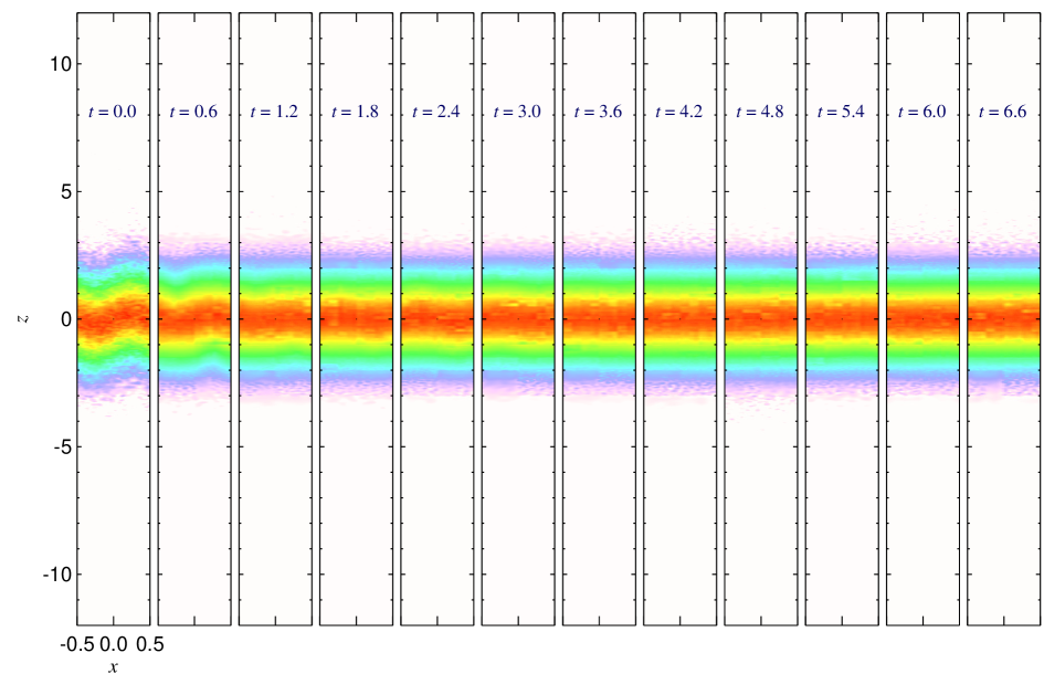
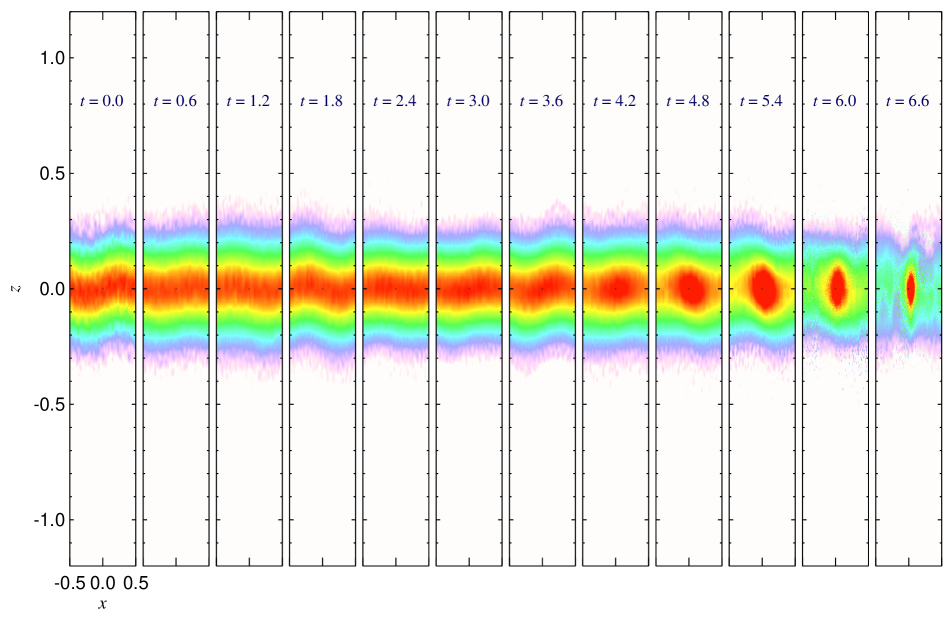
Figure 59: Time evolution of an isothermal gas sheet under self-gravity when periodicity is imposed only in the $x$- and $y$-directions. The upper simulation follows a disk that is thick enough relative to the box width to guarantee that transverse perturbations cannot have a wavelength larger than $2\pi$ times the scale-height, thus it should be stable. In contrast, the sheet simulated in the bottom panel is a factor of 10 thinner in units of the transverse box size, and thus should be prone to instabilities. The stability is tested explicitly by imposing in the initial conditions a weak sinusoidal perturbation with wavelength equal to the box width. This yields results consistent with the theoretical expectations, as the upper simulation settles into a stable sheet, while the lower one breaks up.

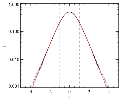
Figure 60: Equilibrium state reached by the ‘thick’ isothermal sheet shown in Figure 59 when compared to the analytic solution (solid red line). The good agreement is an indirect validation of GADGET-4’s gravity solver with mixed boundary conditions. The dashed vertical lines indicate one scale-height below and above the mid-plane.

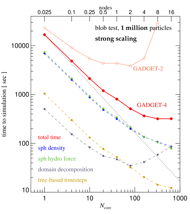
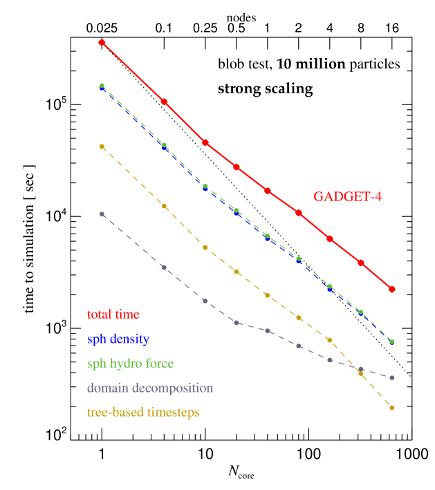
Figure 61: Evaluation of strong scalability and raw computational speed of a pure SPH calculation without self-gravity, the ‘blob test’ analyzed in Agertz et al. (2007). We have used the “Freya” cluster at MPA for these tests (the nodes are equipped with dual Intel Xeon Gold 6138 CPUs, each with 20 physical cores at 2.0 GHz), and the original initial conditions at resolutions of 1 million (left panel) or 10 million (right panel) prepared by Agertz et al. (2007) for the blob test. In both cases, we have run simulations in serial (1 core) and parallel with up to 640 cores (16 full nodes). The filled circles show the wall-clock time consumed by different code parts of GADGET-4 over the full course of the simulation up to time $t=5.0\,\tau_{\rm KH}$ (where $\tau_{\rm KH}$ is the Kelvin-Helmholtz time). The solid red line marks the total elapsed time. Perfect strong scalability corresponds to the dotted line. For the small problem size, strong scaling is lost at around 8 nodes; at this point it does not make sense any more to add more compute resources. The main culprit responsible for this is the domain decomposition algorithm, while the actual SPH calculations still perform well at this point, although imbalance and communication losses also become noticeable. Still, GADGET-4 performs much better than GADGET-2 (open symbols and thin red line), which has been run for comparison with the same set-up and loses scalability much earlier. As is well known, larger problem sizes allow for better scalability in practice. This is explicitly demonstrated in the right hand panel, where the corresponding test results for the simulation with 10 million SPH particles are reported. Here GADGET-4 shows good strong scaling all the way to 640 cores.

9.2 The Santa Barbara cluster

As a further example and useful comparison to other hydrodynamical codes, we use the Santa Barbara cluster simulation, which goes back to a community code comparison effort carried out by Frenk et al. (1999). Since then, the Santa Barbara cluster has repeatedly been used in the literature as an important validation check of cosmological hydro codes, and also as a means to study fundamental issues related to entropy creation and the treatment of mixing in different hydrodynamical discretization techniques. Here we focus on a basic validation test of the cosmological SPH implementation in the GADGET-4 code, by carrying out the Santa Barbara simulation at a set of different resolutions, including $2\times 256^{3}$, which is higher than considered in the original comparison project.

In Figure 56, we show radial profiles of the dark matter density, the gas density, the gas temperature and the entropy of the main cluster halo at $z=0$. We here show the pressure-based formulation of SPH, but note that the density-based formulation gives very similar results. The agreement between different resolutions in the dark matter and gas properties shows the expected systematics. Diverse answers have been reported for the central entropy profile between different hydrodynamical codes (see, e.g., Ascasibar et al., 2003; Springel, 2005; Almgren et al., 2013; Hopkins, 2015; Saitoh & Makino, 2016). The low entropies we find here for SPH in the central cluster region can be interpreted as arising from a low degree of mixing in the central cluster region, likely resulting from an unphysical suppression of turbulent mixing, an effect that tends to be slightly more pronounced in the density-entropy formulation of SPH. Most mesh codes predict considerably higher central entropies, likely too high ones in some cases, as these codes can easily produce excess entropy associated with truncation errors and numerical diffusivity (Mitchell et al., 2009; Springel, 2010a; Vazza, 2011). A number of modifications to SPH have been suggested that also produce entropy cores (Sembolini et al., 2016), but ultimately the correct answer for this problem is not fully established yet.

9.3 Merger-induced starburst

We next consider a simple simulation of a galaxy merger including radiative cooling and star formation, here modelled with the explicit subgrid model introduced by Springel & Hernquist (2003), which is presently the only approach available in GADGET-4 to account for feedback from star formation. For definiteness, we set-up two identical compound galaxy models which have initially $3\times 10^{5}$ particles in the dark matter halo, $1.5\times 10^{5}$ particles in an initial exponential stellar disk, $3\times 10^{5}$ SPH particles for the gas component, and $5\times 10^{4}$ in a central stellar bulge. The virial velocity of the halo is chosen as $160\,{\rm km\,s^{-1}}$, giving the galaxy a total mass close to $10^{12}\,h^{-1}{\rm M}_{\odot}$. We choose a total disk mass fraction of 0.05, with 33% of this in the gas component, the other 66% in the preformed stellar disk. The initial disk scale length is $2.53\,h^{-1}{\rm kpc}$, and we additionally put a mass fraction of 0.02 into a central, spherically symmetric stellar bulge.

The galaxies are set-up in quasi-equilibrium with the MAKENEWDISK code, which implements a method described in Springel, Di Matteo & Hernquist (2005) that can also account for gas pressurized by the ISM model, unlike our more sophisticated GALIC code described in Yurin & Springel (2014). We then put them onto a collision orbit that is parabolic, and has a nominal minimum separation at first encounter equal to $3\,h^{-1}{\rm kpc}$ if the galaxies were point masses. The merger simulation is started when the galaxy centers are $160\,h^{-1}{\rm kpc}$ apart. At this time, the dark matter halos already have started to overlap, but the initial orbit has been corrected such that the galaxies fall together on the same path as if they had started from a still larger separation. We also incline the disks slightly relative to the orbital plane, by 10 and 40 degrees, respectively, making this a prograde merger.

In Figure 57, we show a time sequence of this high-resolution, slightly “wet” galaxy merger. We have used hierarchical time integration here, but the results are essentially invariant with respect to the details of the integration settings. The time evolution shows the typical dynamics of a major merger in $\Lambda$CDM. The galaxies experience a strong tidal shock in their first encounter, which induces tidal arms and drives some gas into the central regions, but also some gas away out of the disks. Due to braking by dynamical friction in the dark matter halos, the galaxies fall together for a second encounter and eventual coalescence. This largely destroys the disks, triggers a moderate starburst, and creates a hot gaseous halo by shock heating some of the gas in the collision.

This evolution is also reflected in the star formation rate, which we show in Figure 58. Globally, the gas is consumed on a consumption timescale of about $1\,{\rm Gyr}$, as illustrated by the dashed line in the figure. The merger modulates this evolution by first triggering an enhancement in the star formation in the first encounter. Eventually, the star formation is diluted while the galaxies linger around at their turn-around radii, before they engage in a second encounter that quickly leads to a full merger. The latter triggers a moderate starburst, before the residual gas in the remnant is consumed again on the consumption timescale of $\sim 1\,{\rm Gyr}$ imposed by the relatively stiff equation of state model used here.

9.4 Isothermal sheet

To demonstrate and validate GADGET-4’s feature to allow self-gravity with periodicity only in two-dimensions, we consider the problem of an isothermal gaseous sheet with periodicity in the $x-$ and $y$-directions, and open boundaries in the $z$-direction. For this case of translational symmetry parallel to the sheet, there is an analytic solution, Spitzer’s isothermal sheet. The density profile in the $z$-direction follows

$$\rho(z)=\rho_{c}\,{\rm sech}^{2}\left(\frac{z}{z_{0}}\right)$$ (118)

with central density $\rho_{c}={\sigma}/({2\,z_{0}})$. The vertical scale height $z_{0}$ is given by

$$z_{0}=\frac{c_{s}}{(2\pi G\rho_{c})^{1/2}},$$ (119)

where $c_{s}$ is the sound-speed, and the gravitational potential relative to the mid-plane of the sheet is given by

$$\phi(z)=2c_{s}^{2}\ln\left[{\rm cosh}\left(\frac{z}{z_{0}}\right)\right].$$ (120)

The isothermal sheet is unstable to perturbations transverse to the $z$-directions if their wavelength exceeds (Ledoux, 1951; Hunter, 1972)

$$\lambda_{\rm crit}=c_{s}\left(\frac{2\pi}{G\rho_{c}}\right)^{1/2}.$$ (121)

This implies $\lambda_{\rm crit}=2\pi z_{0}$. We thus expect that the isothermal sheet can only stay stable if the periodic boxsize in the directions transverse to $z$ is at most $2\pi$ times the scale height.

To verify our gravity solver with periodicity in two out of three dimensions, and to test for this bound, we carry out two simulations. For definiteness we pick a box with dimensions $L_{x}=L_{y}=1$, and $L_{z}=32$. In one of the runs, we adopt a scale-height of $z_{0}=1$ with a surface density of $\sigma=1$, in the other we choose a thinner disk with $z_{0}=0.1$ and $\sigma=0.1$, such that the dynamical timescales of both disks are the same. With these parameters, the thicker disk should be in the stable regime, whereas the thinner is expected to be unstable to perturbation transverse to the $z$-direction. To trigger this potential instability in a controlled fashion, we create the particle positions in the initial conditions by randomly sampling the isothermal sheet and then displacing them around the midplane by $\Delta z(x)=0.2\,z_{0}\sin(2\pi x/L_{x})$.

In Figure 59, we show the time evolution obtained for these two sheets, which can be considered ‘thick’ and ‘thin’ in units of the transverse box size. The expectations on their stability are borne out by the time evolution of the sheets; whereas the initially imposed perturbation in the $z$-direction is dissipated away for the thick sheet, it grows for the thin sheet, leading to a fragmentation of the sheet into a set of spherical blobs.

The equilibrium state assumed by the first sheet accurately follows Spitzer’s isothermal sheet profile. This is illustrated in Figure 60, which compares the SPH particle densities in the final state with the analytic solution. Indirectly this also confirms that the gravity solver produces accurate results for this case of mixed boundary conditions.

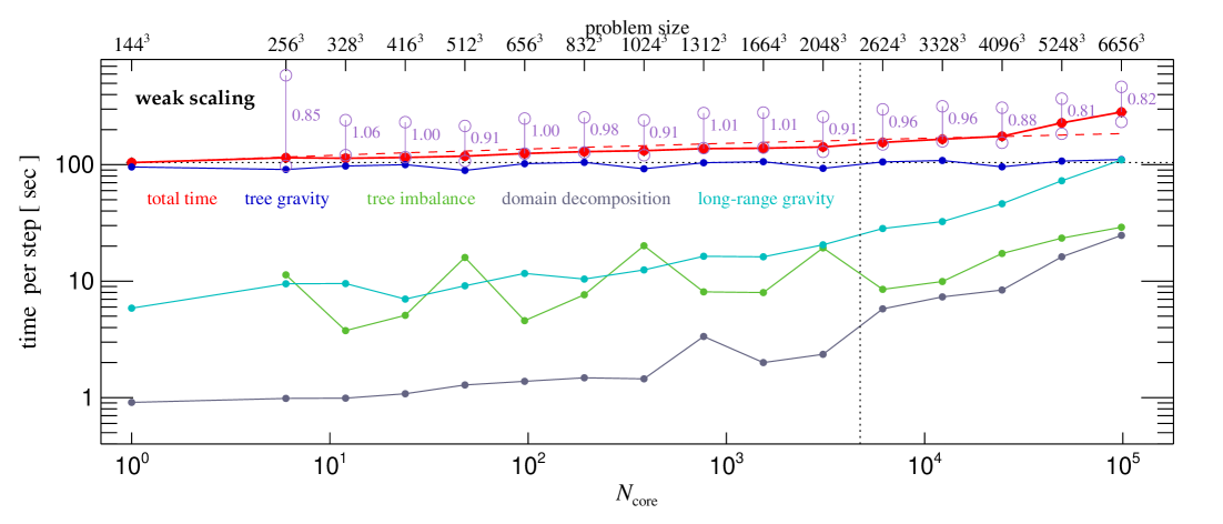
Figure 62: Weak scaling test of GADGET-4 on SuperMUC-NG (which consists of nodes with two 24-core Intel Xeon Platinum 8174 CPUs at 3.1 GHz) at the Leibniz Supercomputing Centre. We hold the load per MPI rank fixed, and run typical cosmological simulations in the high-redshift regime where the box size, particle resolution, and PM-grid size are all increased in lock-step, while the mass resolution is kept fixed. We start with $144^{3}$ particles on a single core, and go all the way to $6656^{3}$ particles on 98304 cores, corresponding to 2048 compute nodes of SuperMUC-NG. The PM grid is always twice the particle grid per dimension, i.e. $288^{3}$ for the smallest test, and going up to $13312^{3}$ for the largest. The different coloured lines show the wall-clock time consumed per step in the most expensive code parts, averaged over three full steps. We see that the most expensive code part, the tree-based short-range force calculation, shows essentially perfect weak scaling over the full range. In particular, the work-load imbalance losses in the tree calculation are negligible compared to the total cost, thanks to the high-quality domain decomposition and our special shared-memory one-sided communication strategy. The domain decomposition and long-range force calculation show a less ideal scaling; towards the largest processor number considered, the PM-force becomes increasingly expensive and will eventually overtake the short-range gravity calculation due to a saturation of the bandwidth of the communication backplane (which for the large partitions suffers from the need to use several islands of the machine with an associated reduction of the available total bisectional bandwidth). Nevertheless, the total cost (red solid line) shows excellent weak scaling, especially when compared to the theoretically expected optimum (red dashed line) that takes into account that the cost of the force calculation algorithm scales as $N\,\log(N)$, where $N$ is the particle number. The two purple hollow circles shown for each processor number $N_{\rm core}$ give, for the lower circle, the total cost assuming perfect weak scaling relative to the previous run with $N_{\rm core}/2$, or for the upper circle, the expected run time if no speed improvement results despite using twice as many cores. The inlined numbers give the fraction of the speed-up that is actually realized by the code thanks to the increase of the number of cores relative to the previous run. Multiplying all these numbers together for the whole scaling series, one obtains 0.37, which can be interpreted as the relative speed of the $10^{5}$ core run with respect to a fiducial speed based on the time needed by the serial code, assuming perfect scalability and ignoring the $\log(N)$ factor in the theoretically expected scaling. If the latter factor is included as well, one obtains 0.66. This means that we see a parallelization loss of only about $33\%$ compared to what is theoretically possible, even though we parallelize here a tightly coupled physical problem over $\simeq 10^{5}$ cores. We consider this to be reassuringly good. Note that by choosing a smaller PM-grid size, the scalability could be improved even further, albeit at the expense of making the tree calculation slightly more costly. Finally, we note that the dotted vertical line marks the simulation size where a slab-based FFT algorithm looses scalability, because for larger problem sizes the number of mesh slabs becomes smaller than the number of processors. Our column-based FFT algorithm used here eliminates this scaling limitation.

10 Code performance and scalability

The quest of achieving maximum computational speed often leads to highly specialized algorithms and computer codes that are only applicable to a particular class of problems. GADGET-4 deliberately aims to be a multi-purpose code that can be applied comparatively flexibly to a range of problem types, without being tied to special hardware. It therefore may not necessarily be the fastest code, but the hope is that it instead excels in reliability and flexibility. But also with these goals in mind, the code still needs to show competitive performance and good scalability to be useful in practice.

In this section we thus examine the scalability of the code for realistic problems, including very demanding ones such as extreme zooms. The latter tend to be harder than tests for uniform particle load, and are arguably more interesting for the methodological goal to allow future simulations to better address multi-scale, multi-physics problems. In the following, we shall first consider the strong scalability of the code for a pure SPH simulation. We then turn to the important problem of weak and strong scalability of homogeneously sampled cosmological dark matter simulations, which is directly relevant for timely studies of cosmic large-scale structure, which increasingly call for very large N-body simulations. We then turn to strong scaling tests of a cosmological hydrodynamical simulation, and finally to a zoom simulation of a Milky Way-sized high resolution dark matter halo.

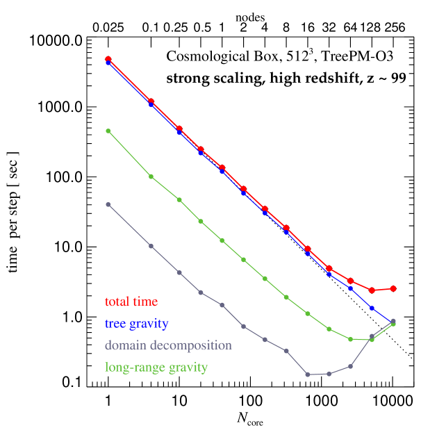
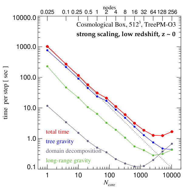
Figure 63: Strong scaling of GADGET-4 for a homogeneously sampled cosmological simulation. As a test simulation, we use a $512^{3}$ run in a $L=100\,h^{-1}{\rm Mpc}$ box. The tests were run on “Cobra”, a large parallel compute cluster operated by the Max Planck Computing and Data Facility. Each node is equipped with two Intel Xeon Gold 6148 CPUs with 20 physical cores at 2.4 GHz. The lowest number of cores we run on is 1 (i.e. we carry it out as a serial calculation), and we extend this up to 10240 cores (256 nodes), using identical code parameters in each case (except for the amount of memory that may be allocated per MPI-rank). As the clustering state changes strongly between the high redshift and low redshift regimes, we examine the scaling in both regimes separately, with high redshift shown in the left panel, and low redshift in the right panel. The reported wall-clock times for different code parts are averaged times per step; at high-$z$ the averaged timestep size is $\Delta\ln a=4.5\times 10^{-3}$, at low-$z$ it is $\Delta\ln a=1.78\times 10^{-4}$. For this problem size, we lose strong scaling slightly below $\sim 10000$ cores, at which point the load per rank has already dropped to $\sim 13000$ particles. The tree calculation still scales at this point, but both the domain decomposition and the PM-mesh calculation (here done with a $1024^{3}$ grid) do not scale anymore for this low load per core.

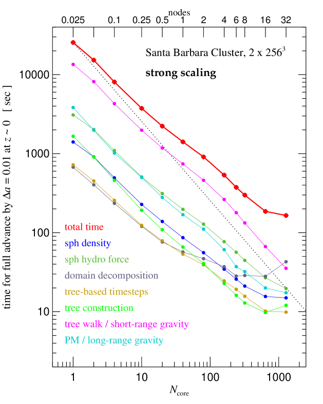
Figure 64: Strong scaling test of the Santa Barbara Cluster (Frenk et al., 1999), using the $2\times 256^{3}$ realization discussed earlier in Fig. 56. We here consider the elapsed time needed in different code parts of GADGET-4 to evolve the simulation at $z=0$ for a time interval corresponding to $\Delta a=0.01$ (i.e. for 1% in expansion factor), which averages over the full timestep hierarchy. We use different numbers of cores on MPA’s “Freya” cluster, starting at a serial computation, and then going parallel by using up to 32 nodes with 40 cores each. We see that for this problem, strong scaling to around 1000 cores is obtained, at which point the domain decomposition starts to spoil further speed-ups when more nodes are added.

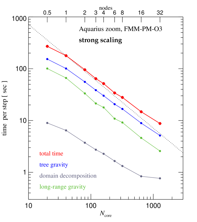
Figure 65: Strong scaling of a high-resolution zoom simulation of a Milky Way-sized dark matter halo on “Cobra”. For definiteness, we consider the Aq-A-2 model of the Aquarius project, at redshift $z\simeq 0.03$, i.e. when the highest degree of clustering is reached. This simulation contains about 607 million particles in total, of which around 184 million are within the virial radius, defined as enclosing 200 times the mean density of the box. The corresponding sphere occupies a fraction of just $3.1\times 10^{-8}$ of the simulated volume, highlighting the extremely inhomogeneous clustering of the particle distribution. We employ the FMM-PM approach with $p=3$ and $N_{\rm grid}=1536$ in this test case, combined with the hierarchical timestepping approach (not because this is necessarily the fastest, but rather just for variety compared to the other tests done previously). The reported times for different code parts are the average wall-clock time per step (which are of size $\Delta\ln a=1.7\times 10^{-5}$) averaged over 3 full cycles through the timestep hierarchy. Clearly, the strong scaling of GADGET-4 for this demanding problem is remarkably good.

10.1 Pure hydrodynamical problem

We here examine a pure SPH problem, the ‘blob test’ of Agertz et al. (2007), in order measure the speed and scalability of the SPH implementation in GADGET-4, with results given in Figure 61. The left panel shows speed measurements in different code parts when the problem is studied with 1 million particles, while the right panel is for the same problem with 10 million particles instead. In this set-up, a cold dense sphere of gas is exposed to a hot, supersonic background wind in order to study the shredding of the clump by fluid instabilities created in the strong shear flow around the clump. Periodic boundary conditions are imposed on all sides of a stretched box, gravity or cooling processes are not included, and ordinary ’vanilla’ SPH is used. We use local timestepping for the integration. The shortest occurring timesteps are about a factor of $\sim 10$ smaller than the longest, so that up to four timebins of the timestep hierarchy are used.

We find that the code shows generally good strong scalability for this problem. Scalability is lost once the load per core has dropped to a few thousand SPH particles, at which point our domain decomposition algorithm becomes too costly in relation to the little work it tries to distribute over more and more shoulders. For a larger problem size, the limit for scalability is accordingly pushed to a larger number of cores (see the right panel). This highlights an important general finding that we expect to be true for all cosmological simulation codes – good scalability to a certain processor number requires a sufficiently large problem size. Importantly, as the direct comparison to GADGET-2 shows (see the left panel in Fig. 61), the new code GADGET-4 is less demanding in this respect than older versions of GADGET, and thus shows a significantly improved scalability.

10.2 Homogeneously sampled cosmological simulations

We now consider the weak scaling of the code for cosmological DM-only simulations. This is shown in Figure 62 for a mass resolution resolution of $m\simeq 5.9\times 10^{8}\,h^{-1}{\rm M}_{\odot}$, carried on the SuperMUC-NG computer at the Leibniz Supercomputing Centre in Garching. In this test, we increase the used partition size, the PM-mesh size, and the size of the particle grid in lock step, such that the particle load per core stays constant. We begin with $144^{3}$ particles on a single core, and proceed up to $6656^{3}$ particles on 98304 cores (which are 2048 compute nodes of SuperMUC-NG). The calculations use the column-based FFT and the TreePM algorithm for $p=3$. The slab-based FFT would be slightly faster (by up to a factor of 2 for the PM part) for low core numbers, but ceases to scale once the number of mesh-planes becomes less than the number of cores, and then quickly loses out against the column-based FFT algorithm.

Overall, the code achieves very good weak scalability. With respect to the theoretically expected mathematical cost of the calculation, which scales as $N\log N$ with particle number $N$, the code realizes a parallel efficiency of about $66\%$ on $10^{5}$ cores relative to carrying out the calculation on a single core, or in other words, a speed-up by a factor of 66000 is reached – despite the coupling of every particle with every other particle through long-range gravity, and despite the fact that the simulations with the largest core sizes have to be spread over several “islands” of the SuperMUC-NG computer, which brings about a significant drop in the available point-to-point communication bandwidth.

Next, we turn to the problem of the strong scalability of a homogeneously sampled cosmological simulation. We examine this for a $512^{3}$ problem size, both for the situation at high redshift close to the initial conditions, and for the highly clustered state at redshift $z=0$, where the code traverses a timestep hierarchy. Results for these tests are shown in Figure 63, again starting at a single core, and now going up to $10^{4}$ cores. Accordingly, the particle load per core drops from more than 134 million to little more than 10000. We find quite good strong scalability of the code for all relevant code parts up to about a load of $10^{5}$ particles per core. Then the domain decomposition starts to increase in cost, and soon seriously impacts further scalability. This would thus be the first target for future work on further improving the scalability of GADGET-4. The angle of attack for this is in fact relatively obvious – unlike the gravitational algorithm itself, the domain decomposition does not yet exploit the fact that typically a sizeable number of MPI ranks runs on a shared-memory node. Instead it assumes the ranks are all on distributed memory-memory machines, making the domain decomposition a more difficult and laborious task than really necessary. Implementing a version of the domain decomposition that takes this hierarchy into account has the potential to speed it up by about an order of magnitude on typical nodes of today’s compute clusters, which would come in handy for pushing the scalability further.

We also note that the scalability of GADGET-4 is rather similar for the TreePM and FMM-PM variants of the force computation algorithms. But of course, the absolute and relative speeds vary depending on the expansion order that is chosen, force accuracy parameter settings, etc. Also note that using an extremely small opening angle for the multipole algorithms can make the relative cost of other code parts irrelevant. This would formally improve the scalability while increasing the overall runtime. In the tests shown here, we have however rather aimed to adopt settings that are typical for production runs with GADGET-4.

Finally, for completeness, we examine a strong scaling experiment for a hydrodynamical cosmological simulation. For definiteness, we consider the Santa Barbara Cluster simulation at a resolution of $2\times 256^{3}$ dark matter and SPH particles. In Figure 64, we show the speed of different code parts when the simulation is evolved in the highly clustered state at $z\sim 0$, through several full cycles of the timestep hierarchy. We consider runs carried out in serial on 1 core and compare with parallel execution on up to 1280 cores. Over this range, good strong scalability can be observed, but it starts to break down at around 1000 cores, again due to the domain decomposition raising its expensive head.

It is interesting to compare these scaling results with other parallel performance measurements reported in the literature for cosmological codes. Recently, Borrow et al. (2018) discussed the strong and weak scaling of the new SWIFT code for cosmological simulations, which employs task-based parallelization controlled with a custom scheduler. For the strong scaling of a problem with $6\times 10^{7}$ particles (hence about twice as large as the Santa Barbara cluster) using 512 cores, they achieve a speed up of $\sim 33.1$ relative to a single-threaded execution. Using a very large particle load of $7\times 10^{6}$ per core, Borrow et al. (2018) report weak scaling to 4096 threads with an overall loss of $25\%$ efficiency. These scaling results appear somewhat worse than what we find for GADGET-4, but their test problem was also characterized by a deep time-step hierarchy. We note, however, that SWIFT has been claimed (Schaller et al., 2016; Gonnet et al., 2013) to offer a substantially higher base speed than GADGET, so it could be a faster code nevertheless, at least for a moderate number of cores.

Our weak scaling results also appear to be better than the ones reported by Wünsch et al. (2018) for the FLASH code. There, even the hydrodynamics shows already a factor of 2 slow-down in a weak scaling to 1536 cores, while this approaches a factor of 10 for the tree-based gravity in FLASH, and is presumably still worse for FLASH’s multigrid gravity solver, judging at least from its relatively limited range of strong scalability.

At face value, our scaling results are also better than the ones reported for CHANGA (Menon et al., 2015), a cosmological N-body code employing the Charm++ framework for task-based parallelization. They also appear better than the weak scaling reported by Harnois-Déraps et al. (2013) for CUBEP3M, who found a weak scaling efficiency of 58% when going from 864 to 21952 cores, a dynamic range in core number of a factor of $\sim 25$, considerably less than the wide dynamic range of $10^{5}$ we have examined here.

Our scaling results are however not as impressive as the ones reported by Habib et al. (2016) for the HACC code framework, who found essentially perfect weak scaling on a BlueGene/Q system up to $1$ million cores. Similarly, Winkel et al. (2012) documented very good weak scalability of their parallel implementation of a tree-code on a BlueGene/P system up to 256000 cores.

10.3 Collisionless zoom simulations

Finally, let us also consider the computational problem of an aggressive zoom simulation. The extreme clustering and much higher dynamic range of such simulations represent a quite demanding regime in which good parallel scalability is far harder to achieve than in homogeneously sampled boxes. As a specific test problem we consider a simulation from the Aquarius project (Springel et al., 2008a), specifically halo Aq-A-2, which we evolve for a couple of full timestep cycles at $z\simeq 0$, when the clustering is strongest. This simulation features about 532 million high resolution particles, of which around one third are contained in the virial radius of a single halo, which occupies far less than a millionth of the simulated volume. In addition, there are about 75 million lower resolution particles of mass progressively growing with distance from the zoomed halo, filling the rest of the volume.

In Figure 65, we show strong scaling measurements with GADGET-4 for this demanding situation, this time using the FMM-PM-O3 algorithm with hierarchical time integration for the sake of showing a variety of tests, not because it scales particularly well (in fact it does not, the Tree-PM variants tend to scale a bit better). We explore the scalability from 20 cores (half a node) to 1280 cores (32 nodes), finding a quite satisfactory strong scaling efficiency over this range. Again, this is a welcome improvement over older versions of GADGET, which do less well for this type of problem.

11 Public code release

More than a decade ago, we described the GADGET-2 code (Springel, 2005), and made it publicly available for download on the internet as a packaged source-code archive file, as it was commonly done at the time. The code had been released as is, and no simple process was foreseen for the community to feedback suggestions for code changes or improvements. In fact, although such developments have happened at many places, such feedback hardly happened, and the public version of GADGET-2 remained essentially static, modulo a relatively small number of fixes.

The development of GADGET continued in a decoupled way from this public version, leading to a major transformation of the code around 2007, and the creation of GADGET-3 (this became the basis of the Aquarius project). Subsequently, a large number of people became involved in developing this code further. Unfortunately, it was never made publicly available and properly documented, but it has been widely shared and distributed by the author upon request. It has also been used as a basis for developing further codes, as described in the introduction section. In recent years, besides our own efforts, two other groups have independently pushed this code to much better scalability, in Munich by Klaus Dolag and collaborators, and in Pittsburgh by Tiziana di Matteo and collaborators. The largely uncoordinated development of GADGET has inspired many creative solutions and enabled a large amount of science, but it also created a fair amount of duplication of effort and a jungle of different versions of GADGET-3 that is quite hard to see through at this point. This of course complicates code validation and the reproducibility of results, and the repetition of effort involved ultimately slows down progress.

With the public release of GADGET-4 through a more modern, collaborative, git-based coding platform that integrates version control, bug tracking, user registration, etc., and the hosting of the code on a standard platform, we hope to be able to avoid this situation in the future. Instead of downloading a static source archive file, users can fetch the source code repository from the version control system that contains the commit history of the code. This has become the standard for most open source software projects, and has also been picked up successfully by other community codes in the field, such as ENZO (Bryan et al., 2014), RAMSES (Teyssier, 2002) , PHANTOM (Price et al., 2018), AREPO (Weinberger, Springel & Pakmor, 2020), among others. We expect this to more easily allow people to contribute suggestions for improvements of GADGET-4 (as a patch or a pull request) that can be integrated into the main code base after approval of a team of moderators. At the same time, users can branch the code for their own private developments, and share these developments with others according to their own policies.

In addition, we have implemented measures in the code that are designed to protect against basic forms of “code rot”, in particular against adding features that are undocumented. If a new feature (controlled through a compile time option) or a new run-time parameter (set through a parameterfile) is introduced, it must be documented as well, otherwise the code will simply refuse to compile with a corresponding error message. This is realized through a special control script as part of the build-process. Likewise, if a documented feature is removed in the actual code, the corresponding documentation needs to be purged as well, so that consistency is always ensured. We hope this simple measure encourages better discipline when modifying the code, and promotes a culture where all code features are always well documented.

The code uses a sophisticated internal memory management system that excludes the possibility of accidental memory leaks while at the same time preventing memory fragmentation. Also, this allows one to always determine precisely how much memory is used, and which code lines are responsible for the different allocations. The code also protects automatically against overuse of the physical memory available on a machine, and hence against the possibility to drive a compute node into swapping (’threshing’). Further stability features include an optional health test upon code start-up that checks for homogeneous CPU-performance across the assigned partition, and evaluates the communication speed between different CPUs. This can for example detect whether a compute node is slowed down by a rogue process (something that can have a huge impact on a parallel job), or whether a single compute node shows reduced network bandwidth that would similarly lead to a skewed performance of the whole run.

Finally, we want to note that we have moved to C++ as default language in GADGET-4, while older versions were written in C. Because this has in part been achieved by modifying older C code, GADGET-4 is hardly in a style that would emerge from redesigning it in C++ from the outset. Still, the code has been segmented in a set of different classes with well defined purposes, and which also hold the code’s data, thereby improving modularity. Inheritance and templating have been used where appropriate to avoid duplication of similar type of code at different places. For example, there is only one basic tree construction routine in the code, and it is used to construct different trees for the gravity calculation, neighbour search, or for computing the potential in the gravitational unbinding in SUBFIND. Also, the tensor arithmetic needed in the higher-order multipole expansions as part of the Tree and FMM calculations can be neatly encapsulated into a corresponding class that supplies tensor objects and overloaded binary operators for doing arithmetic with them. Complicated expressions with tensors can then be expressed very compactly in the code, without any index clutter, thereby greatly improving readability and thus reducing opportunities for coding errors.

12 Discussion and conclusions

In this work, we have described a new version of the GADGET-4 code, which we publicly release to the community. Our goal has been to modernize GADGET-2 from the ground-up, and to provide a reference code that primarily excels in accuracy, versatility and robustness when applied to gravitational dynamics in cosmic structure formation. We hope that this will be a useful code base for numerical cosmology, especially for the high accuracy simulations needed for future large-scale structure work, but also for calculations with very high dynamic range, because the code has been improved significantly in scalability, and in its ability to carry out very large problem sizes.

Compared to previous versions of GADGET, the following features are arguably most noteworthy. The code now offers a Fast Multipole Method as an alternative to a plain tree code, and both algorithms can optionally be run with higher-order multipole moments, or as TreePM or FFM-PM hybrid methods. The FFM approach is momentum conserving and can in some situations be substantially faster at a given force accuracy than the pure tree code. When combined with a new hierarchical time integration scheme for gravity, the manifest momentum conservation of FMM can even be retained for local and adaptive timestepping.

We have improved the domain decomposition algorithm, letting it balance different constraints at the same time and establish an optimum compromise between them. In particular, this prevents memory imbalance as a side-effect of attempts to balance the computational work, which otherwise has often shown up as a problem in past work, especially for zoom-in calculations. For small problem sizes, the cost of the domain decomposition itself is presently usually the limiting factor for strong scalability. However, our current algorithm for the domain decomposition does not yet take note of the fact that easy communication within nodes is possible through the use of shared memory. Rather it subdivides the domains as if each MPI rank lived in a separate distributed memory node. Refining this into a hierarchical approach that takes the mapping of MPI ranks onto shared-memory compute nodes into account has great potential to significantly reduce the cost of the domain decomposition, and thus to extend the scalability of GADGET-4 further.

With respect to smoothed particle hydrodynamics, the new code offers an improved version of vanilla SPH, and as an alternative one flavour of pressure-based SPH. The new code structure allows much easier extension of the SPH routines despite their more sophisticated communication patterns. In particular, GADGET-4 now uses hybrid shared-memory parallelization with an MPI-3 enabled one-sided communication approach, which we think is a promising coding style for the powerful many-core shared-memory nodes that have become the primary building of today’s supercomputers. Efficiency for a large dynamic range is also further supported by the fact that the timesteps of hydrodynamics and gravity can be split, with hydrodynamics subsampling the gravitational dynamics. We note that the public version of the code also contains simple prescriptions for radiative cooling and star formation, which are primarily intended to facilitate the development of improved physics models by interested users.

The improved scalability of GADGET-4 is further assisted by a removal of certain barriers that existed in older versions of GADGET, such as the limits imposed by a slab-based approach to parallel distributed FFTs. The code now offers an optional column based approach that is completely flexible. It also allows arbitrarily stretched boxes, as well as the possibility to restrict the periodicity of gravity to just two dimensions. Other limits that have been addressed and lifted are issues like the former restriction of the halo numbers to 2 billion objects, or the fact that single MPI commands cannot transmit more than 2 billion data elements. The code detects such situations and uses several communication calls if needed.

The code offers for the first time support for built-in merger tree construction and lightcone outputs, optionally also featuring halo identification directly on the lightcone. This promises to make GADGET-4 particularly useful for populating the backwards lightcone with halos and/or galaxies predicted by a suitable model. The built-in power spectrum measurement routines are another feature that should be useful to quickly diagnose and analyse simulation results. Usability of the code is also improved by extensive code performance metrics that are produced and reported during a calculation, and the support of HDF5 output throughout.

In first test applications of the code we have shown that it provides converged solutions for publicly available test problems that are robust to changes of timestepping and force accuracy. Because we can independently demonstrate that the forces are correct and unbiased, we have good reason to believe that GADGET-4 indeed gives correct results when applied carefully, thereby providing reference solutions that may be useful in many scientific applications. With the public release of GADGET-4 we hope to make a useful contribution to the development of more powerful and accurate simulation codes in astrophysics. We would be pleased if this work helps to stimulate further work in this direction.

Data availability

The code discussed in this study has been made publicly available at https://wwwmpa.mpa-garching.mpg.de/gadget4. Data of specific test simulations can be obtained upon reasonable request from the corresponding author.

Appendix A Multipole extensions at different order

The following expressions spell out the potential approximation in our FMM scheme (see subsection 2.4) at different order $p$:

$$\Phi_{p=2}({\bf x}) \simeq -G\left[{Q}_{0}{D}_{0}+\frac{1}{2}{\bf Q}_{2}\cdot{\bf D}_{2}\right.-{Q}_{0}{\bf D}_{1}\cdot{\bf a}\left.+\frac{1}{2}{Q}_{0}{\bf D}_{2}\cdot{\bf a}^{(2)}\right],$$ (122)

$$\Phi_{p=3}({\bf x}) \simeq -G\left[{Q}_{0}{D}_{0}+\frac{1}{2}{\bf Q}_{2}\cdot{\bf D}_{2}+\frac{1}{6}{\bf Q}_{3}\cdot{\bf D}_{3}\right.-({Q}_{0}{\bf D}_{1}+\frac{1}{2}{\bf Q}_{2}\cdot{\bf D}_{3})\cdot{\bf a}+\frac{1}{2}{Q}_{0}\,{\bf D}_{2}\cdot{\bf a}^{(2)}\left.-\frac{1}{6}{Q}_{0}{\bf D}_{3}\cdot{\bf a}^{(3)}\right],$$ (123)

$$\Phi_{p=4}({\bf x}) \simeq -G\left[{Q}_{0}{D}_{0}+\frac{1}{2}{\bf Q}_{2}\cdot{\bf D}_{2}+\frac{1}{6}{\bf Q}_{3}\cdot{\bf D}_{3}+\frac{1}{24}{\bf Q}_{4}\cdot{\bf D}_{4}\right.-({Q}_{0}{\bf D}_{1}+\frac{1}{2}{\bf Q}_{2}\cdot{\bf D}_{3}+\frac{1}{6}{\bf Q}_{3}\cdot{\bf D}_{4})\cdot{\bf a}+\frac{1}{2}\left({Q}_{0}\,{\bf D}_{2}+\frac{1}{2}{\bf Q}_{2}\,{\bf D}_{4}\right)\cdot{\bf a}^{(2)}$$ (124)

$$-\frac{1}{6}{Q}_{0}{\bf D}_{3}\cdot{\bf a}^{(3)}\left.+\frac{1}{24}{Q}_{0}{\bf D}_{4}\cdot{\bf a}^{(4)}\right].$$

$$\Phi_{p=5}({\bf x}) \simeq -G\left[{Q}_{0}{D}_{0}+\frac{1}{2}{\bf Q}_{2}\cdot{\bf D}_{2}+\frac{1}{6}{\bf Q}_{3}\cdot{\bf D}_{3}+\frac{1}{24}{\bf Q}_{4}\cdot{\bf D}_{4}+\frac{1}{120}{\bf Q}_{5}\cdot{\bf D}_{5}\right.-({Q}_{0}{\bf D}_{1}+\frac{1}{2}{\bf Q}_{2}\cdot{\bf D}_{3}+\frac{1}{6}{\bf Q}_{3}\cdot{\bf D}_{4}+\frac{1}{24}{\bf Q}_{4}\cdot{\bf D}_{5})\cdot{\bf a}$$ (125)

$$+\frac{1}{2}\left({Q}_{0}\,{\bf D}_{2}+\frac{1}{2}{\bf Q}_{2}\,{\bf D}_{4}+\frac{1}{6}{\bf Q}_{3}\,{\bf D}_{5}\right)\cdot{\bf a}^{(2)}-\frac{1}{6}\left({Q}_{0}{\bf D}_{3}+\frac{1}{2}{\bf Q}_{2}{\bf D}_{5}\right)\cdot{\bf a}^{(3)}\left.+\frac{1}{24}{Q}_{0}{\bf D}_{4}\cdot{\bf a}^{(4)}\right.\left.-\frac{1}{120}{Q}_{0}{\bf D}_{5}\cdot{\bf a}^{(5)}\right].$$

Explicit forms for the derivatives of $g(r)$ that enter equations (29)-(34):

$$g_{0}(r) = g$$ (126)

$$g_{1}(r) = \frac{1}{r}\,g^{\prime}$$ (127)

$$g_{2}(r) = \frac{1}{r^{2}}\left(g^{\prime\prime}-\frac{g^{\prime}}{r}\right)$$ (128)

$$g_{3}(r) = \frac{1}{r^{3}}\left(g^{\prime\prime\prime}-3\frac{g^{\prime\prime}}{r}+3\frac{g^{\prime}}{r^{2}}\right)$$ (129)

$$g_{4}(r) = \frac{1}{r^{4}}\left(g^{\prime\prime\prime\prime}-6\frac{g^{\prime\prime\prime}}{r}+15\frac{g^{\prime\prime}}{r^{2}}-15\frac{g^{\prime}}{r^{3}}\right)$$ (130)

$$g_{5}(r) = \frac{1}{r^{5}}\left(g^{\prime\prime\prime\prime\prime}-10\frac{g^{\prime\prime\prime\prime}}{r}+45\frac{g^{\prime\prime\prime}}{r^{2}}-105\frac{g^{\prime\prime}}{r^{3}}+105\frac{g^{\prime}}{r^{4}}\right)$$ (131)

$$g_{6}(r) = \frac{1}{r^{6}}\left(g^{\prime\prime\prime\prime\prime\prime}-15\frac{g^{\prime\prime\prime\prime\prime}}{r}+105\frac{g^{\prime\prime\prime\prime}}{r^{2}}-420\frac{g^{\prime\prime\prime}}{r^{3}}+945\frac{g^{\prime\prime}}{r^{4}}-945\frac{g^{\prime}}{r^{5}}\right)$$ (132)

$$g_{7}(r) = \frac{1}{r^{7}}\left(g^{(7)}-21\frac{g^{(6)}}{r}+210\frac{g^{\prime\prime\prime\prime\prime}}{r^{2}}-1260\frac{g^{\prime\prime\prime\prime}}{r^{3}}+4725\frac{g^{\prime\prime\prime}}{r^{4}}-10395\frac{g^{\prime\prime}}{r^{5}}+10395\frac{g^{\prime}}{r^{6}}\right)$$ (133)

In the Newtonian case, we simply have $g_{0}=1/r$, $g_{1}=-1/r^{3}$, $g_{2}=3/r^{5}$, $g_{3}=-15/r^{7}$, $g_{4}=105/r^{9}$, $g_{5}=-945/r^{11}$, $g_{6}=10395/r^{13}$, and $g_{7}=-135135/r^{15}$.

The following expressions for ${\bf D}_{6}$ and ${\bf D}_{7}$ give the next higher order derivatives of the interaction kernel, extending equations (29)-(34):

$$({\bf D}_{6})_{ijklmn} = g_{3}\left[\delta_{mn}\delta_{ij}\delta_{kl}+\delta_{mn}\delta_{jk}\delta_{il}+\delta_{mn}\delta_{ik}\delta_{jl}+\delta_{ln}\delta_{ij}\delta_{km}+\ldots\mbox{(15 terms)}\right]+$$ (134)

$$g_{4}\,\left[r_{l}r_{m}\left(\delta_{ij}\delta_{kn}+\delta_{jk}\delta_{ik}+\delta_{ik}\delta_{jk}\right)+\ldots\mbox{(15 x 3 terms)}\right]+$$

$$g_{5}\,\left[\delta_{ij}\,r_{k}r_{l}r_{m}r_{n}+\ldots\mbox{(15 terms)}\right]+$$

$$g_{6}\,r_{i}r_{j}r_{k}r_{l}r_{m}r_{n}$$

$$({\bf D}_{7})_{ijklmno} = g_{4}\,\left[r_{o}\delta_{ij}\delta_{kl}\delta_{mn}+\ldots\mbox{(15 x 7 terms)}\right]+$$ (135)

$$g_{5}\,\left[r_{o}r_{l}r_{m}(\delta_{ij}\delta_{kn}+\delta_{ik}\delta_{jn}+\delta_{in}\delta_{jk})+\ldots\mbox{(35 triples x 3 kronecker terms)}\right]+$$

$$g_{6}\,\left[r_{i}r_{j}r_{k}r_{l}r_{m}\delta_{no}+\ldots(\mbox{21 terms})\right]+$$

$$g_{7}\,r_{i}r_{j}r_{k}r_{l}r_{m}r_{n}r_{o}$$

References

- Agertz et al. (2007) Agertz O. et al., 2007, MNRAS, 380, 963
- Almgren et al. (2013) Almgren A. S., Bell J. B., Lijewski M. J., Lukić Z., Van Andel E., 2013, ApJ, 765, 39
- Angulo & Pontzen (2016) Angulo R. E., Pontzen A., 2016, MNRAS, 462, L1
- Angulo et al. (2012) Angulo R. E., Springel V., White S. D. M., Jenkins A., Baugh C. M., Frenk C. S., 2012, MNRAS, 426, 2046
- Angulo et al. (2020) Angulo R. E., Zennaro M., Contreras S., Aricò G., Pellejero-Ibañez M., Stücker J., 2020, arXiv e-prints, arXiv:2004.06245
- Ascasibar et al. (2003) Ascasibar Y., Yepes G., Müller V., Gottlöber S., 2003, MNRAS, 346, 731
- Avila et al. (2014) Avila S. et al., 2014, MNRAS, 441, 3488
- Bagla (2002) Bagla J. S., 2002, Journal of Astrophysics and Astronomy, 23, 185
- Balsara (1995) Balsara D. S., 1995, Journal of Computational Physics, 121, 357
- Barnes & Hut (1986) Barnes J., Hut P., 1986, Nature, 324, 446
- Barnes (1990) Barnes J. E., 1990, Journal of Computational Physics, 87, 161
- Barnes & Hut (1989) Barnes J. E., Hut P., 1989, ApJS, 70, 389
- Bauer & Springel (2012) Bauer A., Springel V., 2012, MNRAS, 423, 2558
- Beck et al. (2016) Beck A. M. et al., 2016, MNRAS, 455, 2110
- Behroozi et al. (2015) Behroozi P. et al., 2015, MNRAS, 454, 3020
- Behroozi, Wechsler & Wu (2013) Behroozi P. S., Wechsler R. H., Wu H.-Y., 2013, ApJ, 762, 109
- Behroozi et al. (2013) Behroozi P. S., Wechsler R. H., Wu H.-Y., Busha M. T., Klypin A. A., Primack J. R., 2013, ApJ, 763, 18
- Borrow et al. (2018) Borrow J., Bower R. G., Draper P. W., Gonnet P., Schaller M., 2018, Proceedings of the 13th SPHERIC International Workshop, 44
- Bryan et al. (2014) Bryan G. L. et al., 2014, ApJS, 211, 19
- Capuzzo-Dolcetta & Miocchi (1998) Capuzzo-Dolcetta R., Miocchi P., 1998, Journal of Computational Physics, 143, 29
- Coles & Bieri (2020) Coles J. P., Bieri R., 2020, Computer Physics Communications, 251, 107081
- Creasey (2018) Creasey P., 2018, Astronomy and Computing, 25, 159
- Cullen & Dehnen (2010) Cullen L., Dehnen W., 2010, MNRAS, 408, 669
- Davis et al. (1985) Davis M., Efstathiou G., Frenk C. S., White S. D. M., 1985, ApJ, 292, 371
- de Leeuw, Perram & Smith (1980) de Leeuw S. W., Perram J. W., Smith E. R., 1980, Proceedings of the Royal Society of London Series A, 373, 27
- De Lucia & Blaizot (2007) De Lucia G., Blaizot J., 2007, MNRAS, 375, 2
- Dehnen (2000) Dehnen W., 2000, ApJ, 536, L39
- Dehnen (2002) Dehnen W., 2002, Journal of Computational Physics, 179, 27
- Dehnen (2014) Dehnen W., 2014, Computational Astrophysics and Cosmology, 1, 1
- Dehnen & Aly (2012) Dehnen W., Aly H., 2012, MNRAS, 425, 1068
- Dolag et al. (2005) Dolag K., Vazza F., Brunetti G., Tormen G., 2005, MNRAS, 364, 753
- Dubinski (1996) Dubinski J., 1996, New A, 1, 133
- Dubinski et al. (2004) Dubinski J., Kim J., Park C., Humble R., 2004, New A, 9, 111
- Efstathiou et al. (1985) Efstathiou G., Davis M., White S. D. M., Frenk C. S., 1985, ApJS, 57, 241
- Elahi et al. (2019) Elahi P. J., Cañas R., Poulton R. J. J., Tobar R. J., Willis J. S., Lagos C. d. P., Power C., Robotham A. S. G., 2019, PASA, 36, e021
- Elahi, Thacker & Widrow (2011) Elahi P. J., Thacker R. J., Widrow L. M., 2011, MNRAS, 418, 320
- Evrard et al. (2002) Evrard A. E. et al., 2002, ApJ, 573, 7
- Ewald (1921) Ewald P. P., 1921, Annalen der Physik, 369, 253
- Fosalba et al. (2015) Fosalba P., Crocce M., Gaztañaga E., Castand er F. J., 2015, MNRAS, 448, 2987
- Frenk et al. (1999) Frenk C. S. et al., 1999, ApJ, 525, 554
- Frigo & Johnson (2005) Frigo M., Johnson S., 2005, Proceedings of the IEEE, 93, 216
- Frontiere, Raskin & Owen (2017) Frontiere N., Raskin C. D., Owen J. M., 2017, Journal of Computational Physics, 332, 160
- Fryxell et al. (2000) Fryxell B. et al., 2000, ApJS, 131, 273
- Gaburov & Nitadori (2011) Gaburov E., Nitadori K., 2011, MNRAS, 414, 129
- Garrison, Eisenstein & Pinto (2019) Garrison L. H., Eisenstein D. J., Pinto P. A., 2019, MNRAS, 485, 3370
- Genel et al. (2019) Genel S. et al., 2019, ApJ, 871, 21
- Gingold & Monaghan (1977) Gingold R. A., Monaghan J. J., 1977, MNRAS, 181, 375
- Glimm (1965) Glimm J., 1965, Communications on Pure and Applied Mathematics, 18, 697
- Gonnet et al. (2013) Gonnet P., Schaller M., Theuns T., Chalk A. B. G., 2013, arXiv e-prints, arXiv:1309.3783
- Gouin et al. (2019) Gouin C. et al., 2019, A&A, 626, A72
- Greengard & Rokhlin (1987) Greengard L., Rokhlin V., 1987, Journal of Computational Physics, 73, 325
- Grzybowski, Gwóźdź & Bródka (2000) Grzybowski A., Gwóźdź E., Bródka A., 2000, Phys. Rev. B, 61, 6706
- Habib et al. (2016) Habib S. et al., 2016, New A, 42, 49
- Hadzhiyska et al. (2020) Hadzhiyska B., Bose S., Eisenstein D., Hernquist L., Spergel D. N., 2020, MNRAS, 493, 5506
- Hairer, Lubich & Wanner (2003) Hairer E., Lubich C., Wanner G., 2003, Acta Numerica, 12, 399
- Han et al. (2018) Han J., Cole S., Frenk C. S., Benitez-Llambay A., Helly J., 2018, MNRAS, 474, 604
- Han et al. (2012) Han J., Jing Y. P., Wang H., Wang W., 2012, MNRAS, 427, 2437
- Harnois-Déraps et al. (2013) Harnois-Déraps J., Pen U.-L., Iliev I. T., Merz H., Emberson J. D., Desjacques V., 2013, MNRAS, 436, 540
- Heitmann et al. (2019) Heitmann K. et al., 2019, ApJS, 245, 16
- Henriques et al. (2020) Henriques B. M. B., Yates R. M., Fu J., Guo Q., Kauffmann G., Srisawat C., Thomas P. A., White S. D. M., 2020, MNRAS, 491, 5795
- Hernandez & Bertschinger (2018) Hernandez D. M., Bertschinger E., 2018, MNRAS, 475, 5570
- Hernquist (1990) Hernquist L., 1990, ApJ, 356, 359
- Hernquist, Bouchet & Suto (1991) Hernquist L., Bouchet F. R., Suto Y., 1991, ApJS, 75, 231
- Hernquist, Hut & Makino (1993) Hernquist L., Hut P., Makino J., 1993, ApJ, 402, L85
- Heß & Springel (2010) Heß S., Springel V., 2010, MNRAS, 406, 2289
- Hilbert et al. (2007) Hilbert S., White S. D. M., Hartlap J., Schneider P., 2007, MNRAS, 382, 121
- Hockney & Eastwood (1988) Hockney R. W., Eastwood J. W., 1988, Computer simulation using particles. Taylor & Francis Group, New York
- Hopkins (2013) Hopkins P. F., 2013, MNRAS, 428, 2840
- Hopkins (2015) Hopkins P. F., 2015, MNRAS, 450, 53
- Hosono, Saitoh & Makino (2016) Hosono N., Saitoh T. R., Makino J., 2016, ApJS, 224, 32
- Hu et al. (2016) Hu C.-Y., Naab T., Walch S., Glover S. C. O., Clark P. C., 2016, MNRAS, 458, 3528
- Hu et al. (2014) Hu C.-Y., Naab T., Walch S., Moster B. P., Oser L., 2014, MNRAS, 443, 1173
- Huang et al. (2018) Huang K.-W., Di Matteo T., Bhowmick A. K., Feng Y., Ma C.-P., 2018, MNRAS, 478, 5063
- Huang et al. (2019) Huang S. et al., 2019, MNRAS, 484, 2021
- Hunter (1972) Hunter C., 1972, Annual Review of Fluid Mechanics, 4, 219
- Ishiyama, Nitadori & Makino (2012) Ishiyama T., Nitadori K., Makino J., 2012, in Proceedings of the International Conference on High Performance Computing, Networking, Storage and Analysis, SC ’12, IEEE Computer Society Press, Washington, DC, USA
- Ishiyama et al. (2020) Ishiyama T. et al., 2020, The Uchuu Simulations: Data Release 1 and Dark Matter Halo Concentrations, arxiv:2007.14720
- Jenkins (2013) Jenkins A., 2013, MNRAS, 434, 2094
- Jenkins et al. (1998) Jenkins A. et al., 1998, ApJ, 499, 20
- Jenkins et al. (2001) Jenkins A., Frenk C. S., White S. D. M., Colberg J. M., Cole S., Evrard A. E., Couchman H. M. P., Yoshida N., 2001, MNRAS, 321, 372
- Katz, Weinberg & Hernquist (1996) Katz N., Weinberg D. H., Hernquist L., 1996, ApJS, 105, 19
- Keller et al. (2019) Keller B. W., Wadsley J. W., Wang L., Kruijssen J. M. D., 2019, MNRAS, 482, 2244
- Klypin, Trujillo-Gomez & Primack (2011) Klypin A. A., Trujillo-Gomez S., Primack J., 2011, ApJ, 740, 102
- Knebe et al. (2011) Knebe A. et al., 2011, MNRAS, 415, 2293
- Kodama & Ishiyama (2019) Kodama T., Ishiyama T., 2019, PASJ, 71, 35
- Kravtsov, Klypin & Khokhlov (1997) Kravtsov A. V., Klypin A. A., Khokhlov A. M., 1997, ApJS, 111, 73
- Ledoux (1951) Ledoux P., 1951, Annales d’Astrophysique, 14, 438
- Lee et al. (2021) Lee J. et al., 2021, ApJ, 908, 11
- Maciejewski et al. (2009a) Maciejewski M., Colombi S., Alard C., Bouchet F., Pichon C., 2009a, MNRAS, 393, 703
- Maciejewski et al. (2009b) Maciejewski M., Colombi S., Springel V., Alard C., Bouchet F. R., 2009b, MNRAS, 396, 1329
- Marinacci et al. (2018) Marinacci F. et al., 2018, MNRAS, 480, 5113
- Mazzarini et al. (2020) Mazzarini M., Just A., Macciò A. V., Moetazedian R., 2020, A&A, 636, A106
- McNally, Maron & Mac Low (2012) McNally C. P., Maron J. L., Mac Low M.-M., 2012, ApJS, 200, 7
- Menon et al. (2015) Menon H., Wesolowski L., Zheng G., Jetley P., Kale L., Quinn T., Governato F., 2015, Computational Astrophysics and Cosmology, 2, 1
- Mitchell et al. (2009) Mitchell N. L., McCarthy I. G., Bower R. G., Theuns T., Crain R. A., 2009, MNRAS, 395, 180
- Monaghan (1992) Monaghan J. J., 1992, ARA&A, 30, 543
- Monaghan (1997) Monaghan J. J., 1997, Journal of Computational Physics, 136, 298
- Monaghan & Gingold (1983) Monaghan J. J., Gingold R. A., 1983, Journal of Computational Physics, 52, 374
- Morris & Monaghan (1997) Morris J. P., Monaghan J. J., 1997, Journal of Computational Physics, 136, 41
- Muldrew, Pearce & Power (2011) Muldrew S. I., Pearce F. R., Power C., 2011, MNRAS, 410, 2617
- Murante et al. (2011) Murante G., Borgani S., Brunino R., Cha S. H., 2011, MNRAS, 417, 136
- Naab & Ostriker (2017) Naab T., Ostriker J. P., 2017, ARA&A, 55, 59
- Naiman et al. (2018) Naiman J. P. et al., 2018, MNRAS, 477, 1206
- Navarro, Frenk & White (1997) Navarro J. F., Frenk C. S., White S. D. M., 1997, ApJ, 490, 493
- Nelson et al. (2015) Nelson D. et al., 2015, Astronomy and Computing, 13, 12
- Nelson et al. (2018) Nelson D. et al., 2018, MNRAS, 475, 624
- Nelson et al. (2013) Nelson D., Vogelsberger M., Genel S., Sijacki D., Kereš D., Springel V., Hernquist L., 2013, MNRAS, 429, 3353
- Nori & Baldi (2018) Nori M., Baldi M., 2018, MNRAS, 478, 3935
- Pakmor et al. (2012) Pakmor R., Edelmann P., Röpke F. K., Hillebrand t W., 2012, MNRAS, 424, 2222
- Pelupessy, Jänes & Portegies Zwart (2012) Pelupessy F. I., Jänes J., Portegies Zwart S., 2012, New A, 17, 711
- Pillepich et al. (2018) Pillepich A. et al., 2018, MNRAS, 475, 648
- Potter, Stadel & Teyssier (2017) Potter D., Stadel J., Teyssier R., 2017, Computational Astrophysics and Cosmology, 4, 2
- Power et al. (2003) Power C., Navarro J. F., Jenkins A., Frenk C. S., White S. D. M., Springel V., Stadel J., Quinn T., 2003, MNRAS, 338, 14
- Price (2008) Price D. J., 2008, Journal of Computational Physics, 227, 10040
- Price (2012) Price D. J., 2012, Journal of Computational Physics, 231, 759
- Price et al. (2018) Price D. J. et al., 2018, PASA, 35, e031
- Puchwein, Baldi & Springel (2013) Puchwein E., Baldi M., Springel V., 2013, MNRAS, 436, 348
- Quinn et al. (1997) Quinn T., Katz N., Stadel J., Lake G., 1997, arXiv e-prints, astroph/9710043
- Ragagnin et al. (2020) Ragagnin A., Dolag K., Wagner M., Gheller C., Roffler C., Goz D., Hubber D., Arth A., 2020, arXiv e-prints, arXiv:2003.10850
- Rantala et al. (2017) Rantala A., Pihajoki P., Johansson P. H., Naab T., Lahén N., Sawala T., 2017, ApJ, 840, 53
- Read & Hayfield (2012) Read J. I., Hayfield T., 2012, MNRAS, 422, 3037
- Ritchie & Thomas (2001) Ritchie B. W., Thomas P. A., 2001, MNRAS, 323, 743
- Rosswog (2015) Rosswog S., 2015, Living Reviews in Computational Astrophysics, 1, 1
- Roy, Bouillot & Rasera (2014) Roy F., Bouillot V. R., Rasera Y., 2014, A&A, 564, A13
- Saha & Tremaine (1992) Saha P., Tremaine S., 1992, AJ, 104, 1633
- Saitoh & Makino (2010) Saitoh T. R., Makino J., 2010, PASJ, 62, 301
- Saitoh & Makino (2016) Saitoh T. R., Makino J., 2016, ApJ, 823, 144
- Salmon & Warren (1994) Salmon J. K., Warren M. S., 1994, Journal of Computational Physics, 111, 136
- Schaller et al. (2015) Schaller M., Dalla Vecchia C., Schaye J., Bower R. G., Theuns T., Crain R. A., Furlong M., McCarthy I. G., 2015, MNRAS, 454, 2277
- Schaller et al. (2016) Schaller M., Gonnet P., Chalk A. B. G., Draper P. W., 2016, in Proceedings of the Platform for Advanced Scientific Computing Conference, PASC ’16, Association for Computing Machinery, New York, NY, USA, p. arXiv:1606.02738
- Schaye et al. (2015) Schaye J. et al., 2015, MNRAS, 446, 521
- Schmidt et al. (2018) Schmidt A. S., White S. D. M., Schmidt F., Stücker J., 2018, MNRAS, 479, 162
- Schneider et al. (2016) Schneider A. et al., 2016, J. Cosmology Astropart. Phys., 4, 047
- Schuchart, Kowalewski & Fürlinger (2018) Schuchart J., Kowalewski R., Fürlinger K., 2018, Hpc Asia’18: Proceedings of Workshops of Hpc Asia, 21
- Scoccimarro (1998) Scoccimarro R., 1998, MNRAS, 299, 1097
- Scoccimarro et al. (2012) Scoccimarro R., Hui L., Manera M., Chan K. C., 2012, Phys. Rev. D, 85, 083002
- Sembolini et al. (2016) Sembolini F. et al., 2016, MNRAS, 457, 4063
- Sijacki et al. (2012) Sijacki D., Vogelsberger M., Kereš D., Springel V., Hernquist L., 2012, MNRAS, 424, 2999
- Simpson et al. (2016) Simpson C. M., Pakmor R., Marinacci F., Pfrommer C., Springel V., Glover S. C. O., Clark P. C., Smith R. J., 2016, ApJ, 827, L29
- Skory et al. (2010) Skory S., Turk M. J., Norman M. L., Coil A. L., 2010, ApJS, 191, 43
- Smith et al. (2014) Smith R. E., Reed D. S., Potter D., Marian L., Crocce M., Moore B., 2014, MNRAS, 440, 249
- Springel (2005) Springel V., 2005, MNRAS, 364, 1105
- Springel (2010a) Springel V., 2010a, MNRAS, 401, 791
- Springel (2010b) Springel V., 2010b, ARA&A, 48, 391
- Springel, Di Matteo & Hernquist (2005) Springel V., Di Matteo T., Hernquist L., 2005, MNRAS, 361, 776
- Springel & Hernquist (2002) Springel V., Hernquist L., 2002, MNRAS, 333, 649
- Springel & Hernquist (2003) Springel V., Hernquist L., 2003, MNRAS, 339, 289
- Springel et al. (2018) Springel V. et al., 2018, MNRAS, 475, 676
- Springel et al. (2008a) Springel V. et al., 2008a, MNRAS, 391, 1685
- Springel et al. (2008b) Springel V. et al., 2008b, Nature, 456, 73
- Springel et al. (2005) Springel V. et al., 2005, Nature, 435, 629
- Springel et al. (2001) Springel V., White S. D. M., Tormen G., Kauffmann G., 2001, MNRAS, 328, 726
- Springel, Yoshida & White (2001) Springel V., Yoshida N., White S. D. M., 2001, New A, 6, 79
- Srisawat et al. (2013) Srisawat C. et al., 2013, MNRAS, 436, 150
- Tanikawa et al. (2013) Tanikawa A., Yoshikawa K., Nitadori K., Okamoto T., 2013, New A, 19, 74
- Tanikawa et al. (2012) Tanikawa A., Yoshikawa K., Okamoto T., Nitadori K., 2012, New A, 17, 82
- Teyssier (2002) Teyssier R., 2002, A&A, 385, 337
- Thiébaut et al. (2008) Thiébaut J., Pichon C., Sousbie T., Prunet S., Pogosyan D., 2008, MNRAS, 387, 397
- Tormen, Diaferio & Syer (1998) Tormen G., Diaferio A., Syer D., 1998, MNRAS, 299, 728
- Valdarnini (2012) Valdarnini R., 2012, A&A, 546, A45
- Vazza (2011) Vazza F., 2011, MNRAS, 410, 461
- Vogelsberger et al. (2020) Vogelsberger M., Marinacci F., Torrey P., Puchwein E., 2020, Nature Reviews Physics, 2, 42
- Wadsley, Keller & Quinn (2017) Wadsley J. W., Keller B. W., Quinn T. R., 2017, MNRAS, 471, 2357
- Walch et al. (2015) Walch S. et al., 2015, MNRAS, 454, 238
- Wang et al. (2020) Wang J., Bose S., Frenk C. S., Gao L., Jenkins A., Springel V., White S. D. M., 2020, Nature, 585, 39
- Wang (2021) Wang Q., 2021, Research in Astronomy and Astrophysics, 21, 003
- Weinberger, Springel & Pakmor (2020) Weinberger R., Springel V., Pakmor R., 2020, ApJS, 248, 32
- Wendland (1995) Wendland H., 1995, Advances in Computational Mathematics, 4, 389
- White (1996) White S. D. M., 1996, in Cosmology and Large Scale Structure, Proceedings of the Les Houches Summer School, Schaeffer R., Silk J., Spiro M., Zinn-Justin J., eds., Elsevier Scientific Publishing Company, Amsterdam, p. 349
- Williams (2012) Williams A., 2012, C++ concurrency in action: practical multithreading. Manning Publ., Shelter Island, NY
- Winkel et al. (2012) Winkel M., Speck R., Hübner H., Arnold L., Krause R., Gibbon P., 2012, Computer Physics Communications, 183, 880
- Wünsch et al. (2018) Wünsch R., Walch S., Dinnbier F., Whitworth A., 2018, MNRAS, 475, 3393
- Xu (1995) Xu G., 1995, ApJS, 98, 355
- Yoshikawa & Tanikawa (2018) Yoshikawa K., Tanikawa A., 2018, Research Notes of the AAS, 2, 231
- Yu, Pen & Wang (2018) Yu H.-R., Pen U.-L., Wang X., 2018, ApJS, 237, 24
- Yurin & Springel (2014) Yurin D., Springel V., 2014, MNRAS, 444, 62
- Zhang et al. (2018) Zhang J., An R., Liao S., Luo W., Li Z., Wang B., 2018, Phys. Rev. D, 98, 103530
- Zhu (2020) Zhu Q., 2020, New Astronomy, 101481
- Zhu, Hernquist & Li (2015) Zhu Q., Hernquist L., Li Y., 2015, ApJ, 800, 6