Properties of flares and CMEs on EV Lac: Possible erupting filament

Abstract

Flares and CMEs are very powerful events in which energetic radiation and particles are ejected within a short time. These events thus can strongly affect planets that orbit these stars. This is particularly relevant for planets of M-stars, because these stars stay active for a long time during their evolution and yet potentially habitable planets orbit at short distance. Unfortunately, not much is known about the relation between flares and CMEs in M-stars as only very few CMEs have so far been observed in M-stars. In order to learn more about flares and CMEs on M-stars we monitored the active M-star EV Lac spectroscopically at high resolution. We find 27 flares with energies between $1.6\times 10^{31}$ and $1.4\times 10^{32}$ erg in $\rm H\alpha$ during 127 hours of spectroscopic monitoring and 49 flares with energies between $6.3\times 10^{31}$ and $1.1\times 10^{33}$ erg during the 457 hours of TESS observation. Statistical analysis shows that the ratio of the continuum flux in the TESS-band to the energy emitted in $\rm H\alpha$ is $10.408\pm 0.026$. Analysis of the spectra shows an increase in the flux of the He ii 4686 Å line during the impulsive phase of some flares. In three large flares, we detect a continuum source with a temperature between 6 900 and 23 000 K. In none of the flares we find a clear CME event indicating that these must be very rare in active M-stars. However, in one relatively weak event, we found an asymmetry in the Balmer lines of $\sim 220\,\rm km\,s^{-1}$ which we interpret as a signature of an erupting filament.

1 Introduction

On the Sun, flares and coronal mass ejections (CMEs) are often related and are thought to be caused by the same mechanism. Several studies and observations (e.g. Shibata & Magara, 2011; Aschwanden et al., 2017) confirm that flares are a result of magnetic reconnection leading to the ejection of magnetic energy. For very energetic and long lasting flares, chances of being associated with a CME are high (Compagnino et al., 2017). Flares and CMEs are well correlated to erupting filaments/prominences (Yan et al., 2011). As discussed by Gopalswamy et al. (2003), about $70\%$ of the erupting prominences are associated with CMEs. In most of these events, the prominence material is seen to lag behind the leading edge of the CME. Erupting prominences can occur both in the active regions where they are more clearly visible (Jing et al., 2004) but also in the quiet regions where the emissions are weak since the magnetic field is weaker (Zirin, 1988; Forbes, 2000). It is worth noting that the solar CME rates and properties change over the whole solar cycle and explicitly over time (Mittal et al., 2009).

Flares and CMEs on other stars especially active M dwarfs are of particular interest. This is because these stars stay active for a long time during their evolution and potentially habitable planets orbit at short distances (Dressing & Charbonneau, 2015). Notably, these stars show frequent energetic flaring as compared to the Sun (Vida et al., 2017, 2019b; Howard et al., 2019b; Günther et al., 2020). It has therefore long been thought that they should correspondingly have numerous and powerful CMEs.

As we discuss in the following, it is very important to understand the flare and CME properties on M dwarfs because they play a very important role in the planetary evolution and habitability. Flares are thought to influence prebiotic chemistry or even initiate photosynthesis on planets (Buccino et al., 2006; Airapetian et al., 2016a, b; Mullan & Bais, 2018; Rimmer et al., 2018).

On the contrary, several authors (e.g. Segura et al., 2010; Venot et al., 2016; Tilley et al., 2017; Vida et al., 2017; Howard et al., 2019b) have shown that flares can affect the habitability of planets and that the impact of very large events is far more important than many small ones. For example Venot et al. (2016) examined the influence of the flare on AD Leo in 1985 (Hawley & Pettersen, 1991) that released $10^{34}$ erg in the wavelength region 120 - 800 nm on the habitability of hypothetical planets around this star. They concluded that it would take about 30 000 years until the atmosphere would return to its normal state when exposed to a superflare. In Muheki et al. (2020, hereafter Paper I), we found that such energetic flares may occur very frequently ($\sim$ 1 event per hour) on AD Leo. This means that the atmosphere of a planet orbiting such a star would be in a state of constant change. As pointed out by Vida et al. (2017), such eruptions can erode planetary atmospheres on the long term, and also directly harm life on the surface. On a brighter note, Abrevaya et al. (2020) show that there is chance for survival for a certain fraction of the organisms.

Unlike for flares, detections of CMEs on these stars are sparse. Only a handful of events on M dwarfs have been successfully confirmed as CMEs; in which the velocities of the events were larger than the escape velocities of the stars as detected from the enhancements in the blue wings of the Balmer lines (Houdebine et al., 1990; Vida et al., 2016). On the other hand, understanding the dynamics of CMEs on these stars is of paramount importance in the search for possibly habitable exoplanets. These events present a possible threat to habitability since increased CME activity may enhance planetary atmospheric losses through ion pick up mechanisms (Lammer et al., 2008). Observations of CMEs are therefore important in order to constrain the prediction models (Leitzinger et al., 2014; Odert et al., 2017). Since these events are random, observing active stars for a long time increases the chances of detection. In addition to this, high resolution spectroscopic observations allow for the detection of even the subtle changes in the line profiles of spectra of these objects.

In this paper, we study the properties of flares and search for CMEs on the active M3.5 dwarf, EV Lac which is viewed equator-on ($60^{\circ}$) (Morin et al., 2008) as opposed to AD Leo which is viewed nearly pole-on (Paper I). EV Lac has been a subject of interest in several flare studies on M dwarfs due to its high activity rate.

Photometric studies of EV Lac by Leto et al. (1997) revealed that approximately 4.8 flares occur per day on this star. They also suggested that the flaring activity of this star could be concentrated on a particular longitude. Osten et al. (2010) observed a superflare on EV Lac in the Gamma-ray/ X-ray regime whose flux was 7000 times larger than the star’s quiescent coronal flux along side variability of the Fe K line which is not found in normal stars. They suggested this as evidence for the existence of nonthermal hard X-ray emission during flares and used the $\rm K\alpha$ emission to model the flaring loops obtaining loop heights $\rm\sim 0.1\,R_{\star}$. Time-resolved spectroscopy (R $\sim$ 10 000) of a flare on EV Lac was done by Honda et al. (2018). They found an asymmetry in the blue wing of the $\rm H{\alpha}$ line in each phase of the flare and an absorption feature in the red wing. They suggested that the red absorption component was a result of plasma downflows in the post flare loops. However, the blue asymmetry could not be explicitly explained due to its occurence over the whole flare duration. Vida et al. (2019a) also did a statistical study of the occurence rates of CMEs on M dwarfs using archival data of 25 objects including EV Lac. They found five slow, weak blue wing enhancements and two stronger events with the strongest having a maximum projected velocity of $513\rm\,km\,s^{-1}$.

In order to get more insights on the flare and CME dynamics on active M dwarfs, continuous and persistent observations are important. Here we present findings from the high resolution spectroscopic observations of EV Lac taken between 2016 and 2019. In addition to the spectroscopic observations, we aim to investigate flares on this star using the high signal to noise data obtained with the Transiting Exoplanet Survey Satellite (TESS) mission.

2 Observations

2.1 Spectroscopic observations and data reduction

EV Lac was monitored during the flare-search program of the Thüringer Landessternwarte using the 2-m Alfred Jensch telescope of the Thüringer Landessternwarte Tautenburg. We use the échelle spectrograph with a $2^{\prime\prime}$ slit yielding $\rm R\sim 35\,000$. The spectra cover the wavelength region from 4536 to 7592 Å. Spectra were obtained in various campaigns from 2016-10-10 until 2019-09-04 with an exposure time of 600 s. Observations were typically scheduled for one week per month when the object was visible. In 31 nights of obeservations, we obtained 762 spectra in a total monitoring time of 127 hours. The observation log is presented in Table 6.

The spectra were bias-subtracted, flat-fielded, corrected for scattered light and extracted using standard Image Reduction Analysis Facility (iraf) routines. Wavelength calibration was performed using spectra taken with a ThAr-lamp.

2.2 Photometric observations

EV Lac was also observed by TESS in Sector 16 (2019-09-11 to 2019-10-16) for 457 hours and the calibrated, two-minute cadence simple aperture photometry (SAP) data were downloaded from the Mikulski Archive for Space Telescopes (MAST) site. With its four 10 cm optical telescopes, TESS simultaneously observes a total field of $24^{\circ}\times\,96^{\circ}$ and each camera has four $\rm 2k\times 2k$ CCDs with a pixel scale of 21^′′. The telescope’s detectors are sensitive in the 600 - 1000 nm wavelength range. This matches part of the wavelength range of our spectroscopic observations e.g. $\rm H{\alpha}$.

3 Results and Analysis

3.1 Spectroscopic observations

3.1.1 Light curves and flare identification

We studied the behaviour of three emission lines; $\rm H{\alpha}$, $\rm H{\beta}$ and He i  5876 Å (He i $\rm D_{3}$) from the spectra of EV Lac. The flux variation in H$\alpha$ over the entire period of observations is shown in Fig. 1. The flux of the line was calculated using the sbands package of iraf. Three passbands were used: one for the line, and two for the continua left and right of the $\rm H\alpha$ line. For the line, a passband width of 4 Å was used. The $\rm H\alpha$ line flux was then normalised to the mean of the continuum flux. From Fig. 1, the lightcurve is seen to increase over the observation period. This implies that we observed EV Lac during a minimum and towards the maximum of the activity cycle. The lightcurve is characterised by a lower number of flares in the early phase and the number increases from around HJD = 2458400 (August 2018) till the end of our observing campaigns.

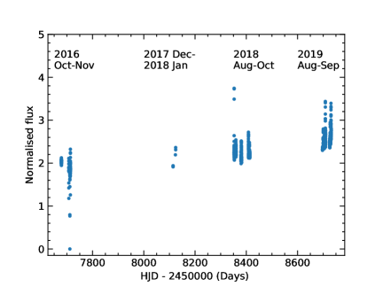
Figure 1: Variation of the $\rm H{\alpha}$ flux of EV Lac over the entire period of spectroscopic observations.

Mavridis & Avgoloupis (1986) proposed a 5-year activity cycle for EV Lac from the long term fluctuation of its quiescent luminosity. Based on this, we predict that EV Lac was at the maximum of its activity cycle in 2019, which explains the higher frequency of flares as compared to the rest of the observing time.

Figure 2 shows examples of the relative flux variation in $\rm H{\alpha}$, $\rm H{\beta}$ and He i $\rm D_{3}$ line of some of the flares. As often observed, the flare lightcurves do not follow a similar trend of a usually fast increase and gradual decay but rather being complex with multiple variations during the decay or even a slow impulsive phase often referred to as slow flares as we shall discuss in section 3.2.1. As indicated in Table 2, in several nights we observed flares only during their impulsive or decay phase. We detected 27 flares in $\rm H{\alpha}$ in the 127 hours of observation which translates to a flare rate of 0.21 flares per hour (5.1 flares per day) with energies $>1.611\pm 0.044\times 10^{31}$ erg. However, it is worth noting that the flare rates depend largely on the activity cycle and therefore may not necessarily explicitly describe the average activity rate of the star.

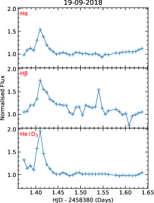
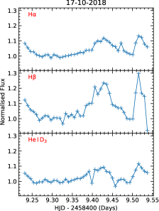
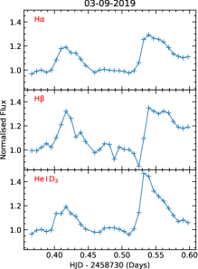
Figure 2: Temporal evolution of flux in the lines showing lightcurves of some of the flares. The top panels show the evolution of $\rm H{\alpha}$ flux, the middle for $\rm H{\beta}$ and the bottom for He i $\rm D_{3}$ of that night.

3.1.2 White-light flares

In this section, we will only discuss the white-light flares observed from spectroscopy. The white-light flares from photometry will be discussed in Section 3.2.1. In most of the nights, we observed no significant change in the continuum during the flares and in quiescence. However, on the nights of 2018 August 21, 2018 September 19, and 2019 September 03 (hereafter, flares F1, F2 and F3 respectively), we observed an enhancement in the continuum at the impulsive phase of the flares and very broadened Balmer lines. These types of flares are known as the Type I white-light flares (Machado et al., 1986). They are thought to arise due to a deposition of energy in the chromosphere by electron beams producing a white-light continuum by hydrogen recombination (Ding & Fang, 1996). The evolution of the white-light flares F1, F2 and F3 is presented in Fig. 3.

To determine the flux enhancement in the continuum in the spectra, we measured the flux of the star in the centre of each spectral order. These values are a measure of the relative flux of the star in each order. The continuum emission of flares has typically a temperature of 10 000 to 20 000 K. Since EV Lac has a temperature of about 3700 K (Gaia Collaboration et al., 2018), the increase of the continuum brightness due to the flare is 6 to 10 times larger at 4600 Å than at 7200 Å . That means, the increase is much larger at the short wavelength than at longer wavelength. By normalising the continuum emission at a wavelength of 7200 Å, we obtain the relative increase of the continuum flux in the spectrum. We thus measured the flux of the spectrum at the middle of each spectral order and normalised these values to 7200 Å. One potential source of error of this method is extinction. However, we observed the change of the continuum brightness in only 3 of the 27 flares and more so during a very brief phase of the flare (see Table 1) and not before or after the event. Since extinction depends on airmass, and we took both pre- and post- flare spectra, we found the effect was very negligible. The spectra were then all normalised to the pre-flare spectrum.

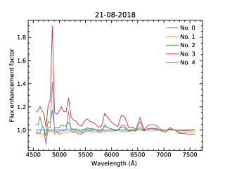
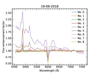
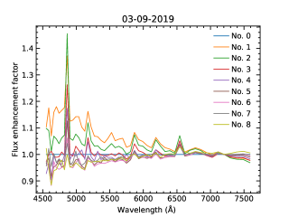
Figure 3: Evolution of the spectra showing the enhancement in the continuum at the impulsive phase of the flares for F1 (top panel), F2 (middle panel) and F3 (bottom panel). The numbers in the legend indicate the spectrum numbers where spectrum No. 0 is the preflare spectrum.

In F2, the enhancement was stronger as compared to F1 and F3 and the enhancement is even much more in the blue in agreement with the classification of white-light flares by Machado et al. (1986). This kind of white-light flares is seen to occur more frequently on the Sun (Ding et al., 1999) as compared to the Type II events. This blue enhancement can be attributed to the emission by $\rm H^{-}$ (Neidig, 1983; Dame & Vial, 1985; Kleint et al., 2016).

Because the continuum flux of a flare can be approximated as a blackbody, we used the relative fluxes to measure the temperature of this blackbody. We did this by fitting a blackbody curve to the relative increase of the continuum. Again, because the increase is much larger at shorter wavelengths than at longer wavelengths, also the fit is dominated by the measurements at the shorter wavelength. For this reason, the blackbody curve is always larger than unity at 7200 Å as shown in Fig. 4. We note that there is a peak at about 4800 Å . This is because there is an emission line close to the centre of that order. However, we do not consider this point in our fit.

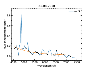
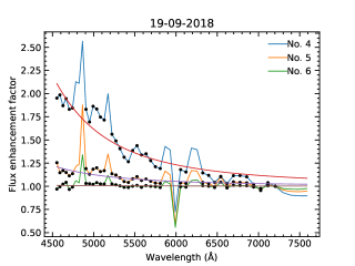
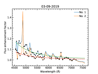
Figure 4: Blackbody fit to the one spectrum showing continuum enhancement in F1 (top panel), three spectra in F2 (middle panel) and two spectra in F3 (bottom panel).

The values of the temperature of the flare and area fraction obtained for the flares is summarised in Table 1.

Table 1: Summary of the values of temperature and area fraction of the white-light flares.

Flare	Spectrum	${t_{o}}/{t}$ (min)a	Temp. (K)	Area
				fraction ($\%$)
2018-08-21	Impulsive	${10}/{260}$	11 600	0.057
2018-09-19	Impulsive	${30}/{360}$	23 000	0.070
	Peak		13 100	0.046
	Decay		6 900	0.020
2019-09-03	Impulsive	${20}/{320}$	14 100	0.030
	Peak		13 300	0.016

^a is the duration of the white-light enhancement relative to the duration of the observation of that night.

3.1.3 Flare energies

The energy released during a flare was estimated by integrating the luminosity over the duration of the flare. In order to determine the absolute line fluxes, we used the flux of each line and its nearby continuum. A flux calibrated spectrum of EV Lac was obtained by scaling the flux calibrated spectrum of AD Leo from Cincunegui & Mauas (2004) to the flux level of EV Lac using the J, H and K brightness measurements given in the SIMBAD database. The flux calibration was done in the same way as in Paper I. We assumed a constant continuum for the flares showing no white light enhancement. However, for the white-light flares, the increase in the continuum was considered. The luminosity was calculated using the flux of the line and the distance of $5.050\pm 0.001$ pc to EV Lac obtained from Gaia (Gaia Collaboration et al., 2018). The energies released in each observed flare are given in Table 2 for $\rm H{\alpha}$, $\rm H{\beta}$ and He i $\rm D_{3}$. In Table 3, we give the energy of the white-light flares taking into account the continuum increase.

Table 2: Summary of the energy of the flares observed in $\rm H\alpha$, $\rm H\beta$ and He i $\rm D_{3}$ in columns 2-4. In columns 5 and 6 are the number of spectra with asymmetries in the blue and the red wings respectively. Columns 7 and 9 represent the maximum line-of-sight velocities observed in that flare in the blue and red respectively. In columns 8 and 10, the average of the line-of-sight velocities of the asymmetries in that flare are also presented.

Date	Flare Energy ($10^{31}$ erg)				No. of spectra			Vel.-Blue ($\rm km\,s^{-1}$)			Vel.-Red ($\rm km\,s^{-1}$)
	Hα	Hβ	He i $\rm D_{3}$		Blue	Red		max.	av.		max.	av.
2016-11-19	3.51$\pm$0.05	$1.065\pm 0.032$	$0.145\pm 0.003$
2018-08-21	6.62$\pm$0.07	$1.626\pm 0.047$	$0.156\pm 0.002$		4	4		179	150		111	108
2018-08-21 †(F1)	3.85$\pm$0.30	1.70$\pm$0.13	$0.112\pm 0.01$		4	4		369	283		450	276
2018-08-22 †	7.20$\pm$0.07	$0.651\pm 0.009$	$0.091\pm 0.001$
2018-08-22 †	$6.082\pm 0.048$	$0.544\pm 0.008$	$0.141\pm 0.002$
2018-09-17	$5.283\pm 0.049$	$1.346\pm 0.025$	$0.125\pm 0.001$
2018-09-17	$4.622\pm 0.051$	$0.618\pm 0.001$	$0.079\pm 0.001$
2018-09-18	9.50$\pm$0.09	$1.423\pm 0.024$	-
2018-09-19 (F2)	11.94$\pm$0.51	$2.093\pm 0.068$	$0.268\pm 0.021$		8	8		410	234		385	218
2018-10-17 †	4.21$\pm$0.05	0.78$\pm$0.01	-
2018-10-17	12.23$\pm$0.10	$2.170\pm 0.037$	$0.267\pm 0.003$
2018-10-17 †	$3.718\pm 0.046$	$0.816\pm 0.040$	$0.104\pm 0.001$
2018-10-20 †	3.17$\pm$0.05	$0.671\pm 0.017$	$0.074\pm 0.001$
2018-10-21	10.45$\pm$0.03	1.87$\pm$0.01	$0.259\pm 0.001$
2019-08-07 †	5.33$\pm$0.05	$1.218\pm 0.018$	$0.102\pm 0.001$
2019-08-07 †	$6.296\pm 0.078$	$1.442\pm 0.026$	$0.140\pm 0.001$
2019-08-08 †	$7.255\pm 0.027$	$1.486\pm 0.007$	$0.159\pm 0.0004$
2019-08-13 †	1.61$\pm$0.04	0.37$\pm$0.02	$0.039\pm 0.002$		2	2		151	148		160	136
2019-08-30	13.71$\pm$0.05	$2.702\pm 0.016$	$0.122\pm 0.001$
2019-08-30 †	$5.758\pm 0.038$	$1.409\pm 0.022$	$0.290\pm 0.001$
2019-08-31 †	10.05$\pm$0.14	$1.943\pm 0.045$	$0.241\pm 0.003$
2019-09-02	$3.777\pm 0.045$	-	-
2019-09-02	6.44$\pm$0.05	-	-		4	4		288	194		88	85
2019-09-03	9.03$\pm$0.21	$1.710\pm 0.058$	$0.189\pm 0.005$		3	3		181	151		109	93
2019-09-03 †(F3)	10.84$\pm$0.22	$2.095\pm 0.044$	$0.26\pm 0.01$		10	10		320	187		280	168

$\dagger$ indicates flares in which only the decay or impulsive phase was observed.

Table 3: Flare energies of the white-light flares taking the continuum increase into account.

Flare		Flare Energy ($10^{31}$ erg)
		$\rm H{\alpha}$	$\rm H{\beta}$	He i $\rm D_{3}$
F1		3.86$\pm$0.30	1.11$\pm$0.13	0.11$\pm$0.01
F2		12.23$\pm$0.66	2.83$\pm$0.10	$0.275\pm 0.024$
F3		10.85$\pm$0.22	$2.278\pm 0.054$	$0.261\pm 0.009$

We calculated the cumulative flare frequency distribution by fitting a cumulative power law to the flares. Since we measured the continuum increase only in three events, the cumulative flare frequency distribution was calculated using the line fluxes without taking the continuum increase into account so that all flares are treated the same way. The cumulative flare frequency distribution follows a power law of the form (Lacy et al., 1976):

$$\log\nu=\beta\log E+b,$$ (1)

where $\nu$ is the number of flares with an energy equal to or greater than $E$ occuring per hour, $\beta$ is the frequency of occurence of flares with various energies and $b$ the y-intercept which sets the flaring rate. The flare frequency distribution can also be expressed as:

$$dN\propto E^{-\alpha}dE,$$ (2)

where $dN$ is the number of flares with energies in the range $[E,E+dE]$. The slope $\beta$ in Eq. 1 and the index $\alpha$ in Eq. 2 are related as $\beta=1-\alpha$. By ignoring flares with energy below $5.28\times 10^{31}$ erg and $1.35\times 10^{31}$ erg in $\rm H{\alpha}$ and $\rm H{\beta}$ respectively in our fit, we obtained $\beta=-1.81\pm 0.21$ and $\beta=-2.58\pm 0.51$ for flares in $\rm H{\alpha}$ and $\rm H{\beta}$ respectively. In Fig. 5, we present the cumulative frequency distribution of EV Lac. We have included the cumulative distribution frequency for AD Leo ($\beta=-1.56\pm 0.13$) obtained from Paper I for comparison. Comparing the distributions of the two stars, we find that AD Leo is on average more active than EV Lac by a factor of $\sim 3$.

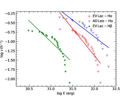
Figure 5: Cumulative flare frequency distribution of flares on EV Lac in H_α (red plus symbols) and H_β (green filled circles). For comparison, AD Leo (Paper I) is also shown in blue tri symbols. The solid lines represent our best linear least-squares fit to each of the Flare Frequency Distributions.

A study of the flare rates in cool stars by Gizis et al. (2017) indicates that using a linear fit to describe the cumulative flare frequency distribution may yield errors since the distribution is usually tailed. They suggested the use of the maximum likelihood estimation to estimate the parameter $\alpha$. We therefore also applied the maximum likelihood estimation to determine the $\beta$ values since the two indices are related as discussed above. The values obtained are summarised in Table 4. The $\rm H\alpha$ energies of the flares are on average a factor $5.27\pm 0.40$ higher than in $\rm H\beta$ and a factor $50.92\pm 8.23$ higher than in He i $\rm D_{3}$. These factors were derived from the energies of the flares whose entire evolution was observed.

Table 4: Summary of the $\beta$ values obtained by least-squares fitting (l.s.f) and maximum likelihood estimation (m.l.e). Columns 2 and 3 correspond to the flares from the Balmer lines and column 4 is the white-light flares from TESS.

Method		$\beta$ value
		$\rm H{\alpha}$	$\rm H{\beta}$	TESS
$\rm l.s.f$		$-1.81\pm 0.21$	$-2.58\pm 0.51$	$-1.78\pm 0.17$
$\rm m.l.e$		$-1.96\pm 0.55$	$-2.71\pm 0.94$	$-2.63\pm 0.82$

The value of b obtained from Eq.1 is $56.81\pm 5.33$, $79.22\pm 5.97$ and $56.48\pm 4.86$ for $\rm H\alpha$, $\rm H\beta$ and TESS respectively.

3.1.4 An erupting quiescent filament and line asymmetries

We searched for line asymmetries to detect CMEs. This was done by subtracting an average spectrum in quiescence of each night from all the night’s flare spectra. The maximum line-of-sight velocity was then estimated at the point where the residual profile merges with the continuum. A clear signal of a CME would be a blue shifted component in the emission line with a line-of-sight velocity greater than the escape velocity of the star. For EV Lac, the escape velocity is $\approx 620\,\rm km\,s^{-1}$.

During the flare evolution, the lines are also broadened especially at the impulsive phase and early decay phase of the flare. This could likely be due to Stark broadening effect as a result of the pressure from the electrons (Švestka, 1972).

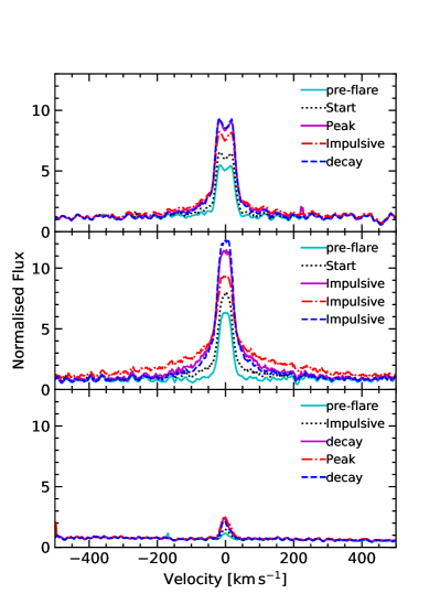
Figure 6: Evolution of the flare F1 showing the asymmetries in the blue and red wings at flare peak in $\rm H{\alpha}$ (top panel), $\rm H{\beta}$ (middle panel) and He i $\rm D_{3}$ (bottom panel).

Figure 6 shows part of the flare evolution of the white-light flare F1 in $\rm H\alpha$, $\rm H\beta$ and He i $\rm D_{3}$. This flare shows asymmetries (both in the blue and the red). We observed only the impulsive phase of this flare and it is seen to peak at different times in the different lines. At the impulsive phase in all the lines, a red asymmetry is observed and at the flare peak the lines are symmetrically broadened. The maximum line-of-sight velocities obtained for the different flares can be found in Table 2. The velocities in the blue component obtained in all flares are all far below the escape velocity of the star (cf Table 2).

As has been discussed by previous studies (e.g. Crespo-Chacón et al., 2006; Leitzinger et al., 2014; Fuhrmeister et al., 2018; Vida et al., 2019a), such low velocity asymmetries have been observed on the Sun and other stars. They are thought to originate from flare plasma motions such as chromospheric evaporations and condesations. Observations of asymmetries on the Sun indicate that mass motions can have velocities in the order of a few tens of $\rm km\,s^{-1}$ (Tei et al., 2018) and the most explosive extend to a few hundreds of $\rm km\,s^{-1}$ (e.g. Canfield et al., 1990). Another possible explanation for the asymmetries is the detection of erupting filaments as have been observed on the Sun.

CMEs often show a three part structure: the bright front that corresponds to the ejected material at the highest speed, the dark cavity carrying intense magnetic fields and the filament which travels at a lower speed (Illing & Hundhausen, 1986). According to Zhang et al. (2001), CME eruptions on the Sun follow phases of initiation, acceleration which coincides with the impulsive phase of the associated flare and propagation where a constant speed is observed. The impulsive acceleration of the CME at the impulsive phase can be attributed to the erupting material in the filament (Kundu et al., 2004). However, a filament is much slower than the CME. The velocities of such eruptions have been found to lie in the range of few tens to hundreds of $\rm km\,s^{-1}$ e.g. Gopalswamy et al. (2003) found events with an average speed of $64.5~{}\rm km\,s^{-1}$ up to $\approx 380\,\rm km\,s^{-1}$ and even higher $\approx 650\,\rm km\,s^{-1}$ (Kundu et al., 2004). This range fits well with the velocities obtained in our observations. It is probable that we observe erupting filaments that occur during the early phase of the eruption.

The spectra in the night of 2019 September 2 (see Fig. 7) shows a blue asymmetry corresponding to a line-of-sight velocity $\approx 220\,\rm km\,s^{-1}$ during a weak and slow flare which was detected only in $\rm H{\alpha}$. Such weak flares have an early thermal phase, when a filament is erupting, that may involve some weak $\rm H{\alpha}$ emission (Bai & Sturrock, 1989).

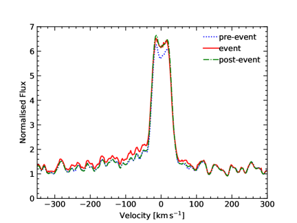
Figure 7: One of the spectra of the night in which no typical flare was observed but blue asymmetry in the continuum was observed in $\rm H{\alpha}$.

These occur in quiet regions where the density of the plasma and the strength of magnetic fields is lower than in the active regions. This kind of erupting filaments has been found to contribute to a reasonable fraction of CMEs on the Sun (Jing et al., 2004; Gosain et al., 2016). This implies that CMEs may not always be associated with only very large flares. We therefore interpret this asymmetry as a signature of an erupting quiescent filament. However, it should still be noted that we did not detect the CME that could have been associated with it.

3.1.5 Detection of the He ii 4686 Å line

In two of the spectra in F2 (indicated as spectrum No. 4 and No. 5 in the middle panel in Fig. 3) and in one spectrum (No. 2 in the bottom panel of Fig. 3) in F3 we detected the He ii 4686 Å line which has only been previously detected in hotter stars since it occurs at very high temperatures $\rm>30\,000\,K$ (Zirin, 1988; Lamzin, 1989). This implies that a continuum source at $\sim 20\,000$  K cannot produce the He ii 4686 Å line. The short duration of the line appearance indicates that such high temperatures are only present during a relatively short time. As discussed by Zirin (1988), strong He II lines are observed in very hot prominences. In such prominences, the ratio of $\rm Ly\alpha$ to $\rm H{\alpha}$ is close to unity. This makes it possible to relate the $\rm H{\alpha}$ flux to the UV radiation. We also detected several other chromospheric lines as discussed in section 3.1.6.

3.1.6 Identification of other chromospheric lines

From the spectra of F2 and F3 in which we observed the He ii 4686 Å line, we produced a list of the emission lines observed during the flares in addition to the three lines under analysis. Flares F2 and F3 are hotter than flare F1. For this reason, F1 does not contain any additional lines that were not already detected in F2 and F3. For example, the He ii 4686 Å line is only seen in F2 and F3 not in F1. The list of the lines is presented in Table 5. Some of these lines have been observed during flares on other stars (e.g. Montes et al., 1999, 2004; Paulson et al., 2006; Fuhrmeister et al., 2011). In Table 5, we also present the non-flare parameters of the lines that are also observed in quiescence using the pre-flare spectrum of the night of 2018-09-19. The Mg i lines are also present only during the flares. Several iron and helium lines are detected in these spectra, most of them occuring only at the flare peak. The observed increase in the Fe i lines suggests that the photosphere was heated during the flares as has been observed on the Sun (Jurčák et al., 2018).

Table 5: Other chromospheric emission lines detected during flares on EV Lac. The wavelengths reported are the observed wavelengths in air as adopted from Moore (1945) and Kramida et al. (2019). N represents the energy of the lines in quiescence emitted in 600 s.

Ion	Wavelength (Å)	Multiplet	Energy ($10^{28}$ erg)
			F2	F3	N
Fe i	5269.54	15	13.06	-	-
	5270.36	37	7.72	-	-
	5318.05	406	4.89	4.84	4.05
	5328.04	15	7.95	-	-
	5371.49	15	7.72	-	-
	5793.93	1086	7.93	5.31
Fe ii	4549.467	38	10.03	5.70	-
	4583.829	38	16.28	8.68	-
	4629.34	37	4.98	-	-
	4666.75	37	3.51	-	-
	4923.921	42	36.87	31.0	-
	5018.434	42	24.24	19.85	-
	5169.03	42	32.55	16.35	5.08
	5197.57	49	7.60	-	-
	5234.62	49	11.51	-	-
	5275.97	49	9.58	-	-
	5316.609	49	22.01	16.44	-
	5325.39	49	3.11	-	4.79
	5362.86	48	8.80	7.42	6.93
	6238.38	74	1.96	1.56	-
	6247.56	74	2.34	2.57	-
	6506.33	blend	37.93	39.53	37.12
He i	4921.9313	48	12.32	13.88	6.68
	4713.14, 4713.34	12	7.92	9.66	-
	5015.678	4	17.05	17.37	9.86
	5875.65	11	41.30	28.61	23.81
	6678.151	46
	7065.04	10
He ii	4685.8308	1	23.14	15.87	-
Mg i	5167.321	2	19.32	7.75	-
	5172.684	2	15.83	8.03	-
	5183.604	2	16.55	6.57	-
Na i	5889.85	1	16.51	7.34	4.65
	5895.92	1	16.04	6.41	3.55
V ii	4928.62	29	9.97	15.69	12.28
Ti ii	4571.971	82	5.47	-	-
H i	4861.332	1	243.60	226.35	187.41
	6562.817	1	1324.79	1044.04	868.10

It is possible to derive several properties of the flares from these lines. Detection of the He ii requires temperatures above 30 000 K and has so far been detected only in hot stars (e.g. Groh et al., 2008). Different diagnostics can be used to distinguish flares from prominences using the ratios of the lines. Waldmeier (1951) classified prominences according to the strength of the magnesium lines to the Fe ii 5169 line. However, according to this classification, active prominences and flares would fall in the same class and are thus not easily distinguished.

According to Tandberg-Hanssen (1963), limb flares can be distinguished from active prominences using the ratio of the Fe ii 5169 Å  line and Ti ii 4572. In flares, the intensity in the Ti ii 4572 $\leq$ Fe ii 5169 and the Fe ii lines of the multiplet no. 42 gets stronger than in the other lines in the multiplets of 37 and 38. This is clearly observed from the line fluxes presented in Table 5.

3.2 Photometric observations

3.2.1 Light curve and flare identification

The TESS lightcurve of EV Lac shows a modulation that we interpret to be due to two starspots (see Fig. 8) located at opposite longitudes as suggested by Morin et al. (2008). It is possible to estimate the properties of these spots following the method of Notsu et al. (2019). The temperature of the spots, $T_{\rm spot}$ can be determined from

$$T_{\rm spot}=T_{\rm star}-3.58\times 10^{-5}T^{2}_{\rm star}-0.249T_{\rm star}+808,$$ (3)

where $T_{\rm star}$ is the temperature of the star. Using the temperature of the star from Gaia (3 742 K), and Eq. 3, we obtained a spot temperature of $\rm\sim 3\,120\,K$. It is then possible to estimate n, the ratio of the temperature of the spot to that of the star. We obtained a value of n = 0.833 which is in agreement with the range of values considered by Jackson & Jeffries (2013). The spot area can then be calculated using

$$A_{\rm spot}=\frac{\Delta F}{F}A_{\rm star}[1-n^{4}]^{-1},$$ (4)

where $\frac{\Delta F}{F}$ is the normalised amplitude variation of the brightness due to the spot. We obtain a spot area of $\approx 4.8\%$ of the area of the star. This agrees well with previous studies on spot coverage on other active M dwarfs (e.g. Howard et al., 2019a).

Using Fourier fitting with Period04 (Lenz & Breger, 2005), we obtained a frequency of $0.233\pm 0.001\,\rm d^{-1}$ which translates into a rotation period of $4.297\pm 0.017$ days, in good agreement with previous studies 4.375 days (Pettersen et al., 1984) and 4.378 days (Pettersen, 1980; Roizman, 1984).

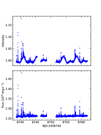
Figure 8: Light curves of EV Lac. The top panel shows the modulation of the light due to starspots while the lower panel is the flux calibrated lightcurve.

A least squares model, F(t) of the form

$$F(t)=z+A_{i}\sum_{i}2\pi\omega_{i}+\phi_{i},$$ (5)

where $z$ is the zero point, $A$ the amplitude, $\omega$ the frequency and $\phi$ the phase all obtained using Period04 was fit to the data and used to normalise the lightcurve (see Fig. 8).

Flares in the lightcurve were identified by visual inspection. 49 flares were identified with some showing fast increase and gradual decay whereas others show a slow rise and decay features as seen in Fig. 9.

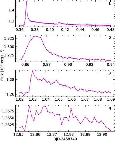
Figure 9: Some of the flare lightcurves that show the diverse nature of flare lightcurves on EV Lac. Panel 1 is the lightcurve of the largest flare that was detected from the TESS observations.

These two types of flares usually referred to as fast (e.g. panel 1, Fig. 9) and slow (e.g. panel 2, Fig. 9) flares, respectively have previously been observed on this and other stars (e.g. Dal & Evren, 2010, 2012; Kowalski et al., 2011; Davenport et al., 2014). White-light fast flares have been described as flares which have rise times less than 10 minutes and slow flares as those whose rise time can last $\sim$ 30 minutes (Dal & Evren, 2010). Fast flares are usually characterised with higher energy as compared to slow flares. According to Gurzadian (1988), slow flares are dominated by thermal emission processes whereas in their counterparts, the dominant source of energy are non-thermal processes. Dal & Evren (2010) found that for EV Lac, $75\%$ of the white-light flares are slow events while $25\%$ are fast flares. Using the classification of Dal & Evren (2010), $\sim 47\%$ of the flares we detected can be classified as slow while $\sim 16\%$ were fast events. The rest ($37\%$) could not easily be classified and so we term them complex flares as suggested by Davenport et al. (2014).

We evaluated the connection of starspots to occurence of flares by phase folding the lightcurve using the obtained rotation period ($4.297\pm 0.017$ days). We used the following ephemeris to fold the lightcurve:

$$BJD=2458738.65769+4.2969E.$$ (6)

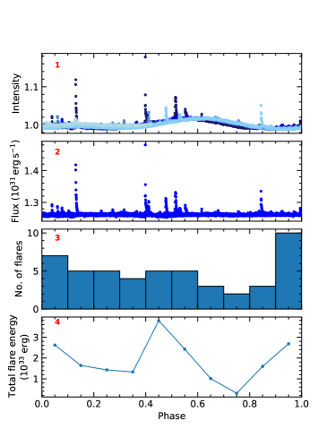
Figure 10: Panel 1 shows the phase folded lightcurve. The different colours represent different cycles and the colours brighten with BJD. Panel 2 is the flux calibrated phase folded lightcurve. Panel 3 is a histogram showing the flare occurence of flares in different phases. Panel 4 shows the variation of the total flare energy per bin.

Flares were seen to occur at all phases as can be seen in Fig. 10. This can be related to the presence of polar spots on this star which may influence the occurrence of flares. According to (Doyle et al., 2018), these spots may interact with multiple spotgroups which lead to constant flaring on this and other M stars at all rotational phases. However, it was observed that the frequency of flares with low energy is higher at the lightcurve minimum at phase 0.9 where surface spottedness is high. This is in agreement to findings by (Roettenbacher & Vida, 2018). They suggest that weak flares appear to occur more often around the starspots probably because they are not strong enough to be seen over the stellar limb. On the other hand, we observed some strong flares at lightcurve minimum but most appear towards the lightcurve maximum (phases 0.4-0.6). This is similar to the patterns reported by (Vida et al., 2016, 2017) on V374 Peg and Trappist-1 objects which are both fully convective M stars. Therefore there is no one-to-one correspondence between brightness of the star and the flare activity, the situation is more complicated. This means that flares do not necessarily come from the region which contains the largest spots, because also the topology of the spot region plays a role for the flare activity.

3.2.2 Flare energies

The flare energies were determined by integrating the luminosity over the whole flare duration. To obtain the luminosity, we multiplied the normalised flux by the quiescent stellar luminosity. The flux of EV Lac in the TESS band was determined from the brightness of the star in the photometric bands convolved with the TESS response function. We obtained the intensity, $\rm I_{\star}=4.135\times 10^{-9}\,erg\,s^{-1}\,cm^{-2}$. The observed luminosity was then estimated using the distance to EV Lac as $\rm 1.262\times 10^{31}\,erg\,s^{-1}$.

As discussed in section 3.1.3, flares follow a power law distribution. In Fig. 11 we show the cumulative flare distribution of flares from the TESS observations in comparison with those observed in $\rm H{\alpha}$. We obtain $\rm\beta=-1.78\pm 0.17$ and $-2.63\pm 0.82$ from the linear fit and the maximum likelihood estimation respectively. Previous photometric studies of EV Lac give values quite lower than those obtained here e.g, ($-0.60\pm 0.11$,  Lacy et al., 1976), ($-0.69\pm 0.12$,  Leto et al., 1997). However, our value of $\beta$ is in good agreement with the values ($\beta\sim-2.05$) obtained by Ilin et al. (2019) for stars of spectral types M3.5 - M5.5 in open clusters. Similarly, Howard et al. (2019b) obtained a value of $\beta=-1.25$ for active M3 dwarfs. All these values are obtained from a linear fit to the flare frequency distribution. The divergence in the values from the former studies could be due to a better sampling of high energy events in this work as compared to the previous studies since the passband used may influence the detection threshold.

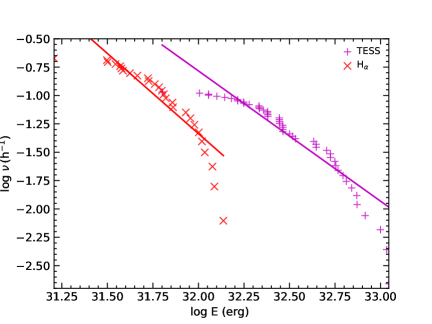
Figure 11: Cumulative flare frequency distribution of flares observed by TESS in comparison with those observed in $\rm H{\alpha}$.

We also calculated the ratio between the continuum flux in the TESS band and the flux in the $\rm H{\alpha}$ line to be $10.408\pm 0.026$. This is in agreement with previous studies (e.g. Somov, 1992) who estimate a factor of 10 between the optical continuum and the $\rm H{\alpha}$ line fluxes for solar flares. We acknowledge that TESS is red sensitive and since the continuum source is $\sim 10\,000-20\,000$ K, only $20-30\%$ of the total continuum emission is in the TESS band.

4 discussion

As discussed in section 3.1.4, we observed several asymmetries in the Balmer lines. These can possibly be interpreted as due to flare plasma motions or erupting filaments at the impulsive phase of the flare. If we consider the latter explanation, we note that we did not observe the fast events that would be associated with them. Instead the velocities reduce as the flare evolves.

Previous studies (e.g. Alvarado-Gómez et al., 2018, 2019) have suggested that the fast events could be suppressed by the strong magnetic fields on these active stars and thus material does not leave the surface of the star. These kind of eruptions are known as failed eruptions since the magnetic field lines do not open up and the filament bounces back.

On another hand, Odert et al. (2020) aimed to establish the potentially observable CME rates for stars of different spectral types and the minimum required observing time to detect stellar CMEs in Balmer lines. They suggested that CME detection is favoured for mid- to late-type M dwarfs because they have a larger fraction of the observable to intrinsic CMEs. However, these stars may require longer observing times >100 hours to detect at least one CME. We observed EV Lac for 127 hours which could have increased our probability of detecting atleast one CME, however these were not continuous observations and thus presenting a constraint.

CMEs expand during propagation and this leads to a decrease in the density of the plasma which could limit the duration during which a signal would be detected. This implies that if the density drops by a large factor, the CMEs become optically thin very quickly to be detected. This could also explain why we do not observe the fast events even if they managed to escape the large scale magnetic field.

We have studied the properties of flares and CMEs on EV Lac which is viewed equator-on and on AD Leo in Paper I which is viewed nearly pole-on since both stars are similar in activity. We note that the viewing angle of the star might not be a constraint in observing CMEs on these stars since the properties of the observed asymmetries are similar.

5 conclusions

We have studied the properties of flares and CMEs on EV Lac and on AD Leo in Paper I because both stars are similar in activity however with different viewing angles. When we observed EV Lac, it was a factor of 3 less active than AD Leo. From the spectroscopic and photometric studies of EV Lac, we detected 27 flares (0.21 flares per hour) in $\rm H{\alpha}$ in the energy range $1.61\times 10^{31}\,-\,1.37\times 10^{32}$ erg and 49 flares ($\approx$ 0.11 flares per hour) from the TESS lightcurve with energies of $6.32\times 10^{31}\,-\,1.11\times 10^{33}$ erg. A rotation period of $4.297\pm 0.017$ days was obtained from the TESS lightcurve. Most of the flares show a complex lightcurve both in spectroscopic and photometric observations and no direct correlation between flaring and starspots was found. Statistical analysis between the energies of the flares observed with TESS and those obtained from the spectroscopic observations shows that the ratio of the continuum flux in the TESS passband to the energies emitted in $\rm H\alpha$ is $10.408\pm 0.026$.

Power-law index $\beta$ values in the range $-1.78\pm 0.17\,-\,-2.58\pm 0.51$ from a linear fit of the cumulative flare frequency distribution and $-1.96\pm 0.55\,-\,-2.71\pm 0.94$ using the maximum likelihood estimation were obtained. Three white-light flares were detected in the spectra of EV Lac. From these flares, it was determined that the area of the emitting region is very small ($\leq 0.07\%$) of the area of the star. At the peak of two of these flares, we also detected the He ii 4686 Å  line which is known to occur only in very hot plasma. Its short appearance at the flare peak indicates that the high plasma temperatures are present only for a short time. Additional chromospheric lines present during the flares were also identified.

We also analysed the spectra by studying the behaviour of the chromospheric lines $\rm H{\alpha}$, $\rm H{\beta}$, and He i $\rm D_{3}$ to detect CMEs. We observed asymmetries in several spectra nearly all of them showing both blue and red wing asymmetries. All the blue wing asymmetries have velocities much smaller than the escape velocity of the star. These slow velocity events may be indicative of the rarity of CMEs on these stars. However, in one relatively weak event, we found an asymmetry in $\rm H\alpha$ of $\sim 220\,\rm km\,s^{-1}$ which we interpret as a signature of a quiet region erupting filament. We however note that the fast event associated with the erupting filament was not detected even if we assume that it could have originated from a quiet region. From these asymmetries, we conclude that the viewing angle may not constrain the detection of CMEs on M dwarfs since the properties of the asymmetries observed in EV Lac are similar to those on AD Leo.

The slow events could be due to suppression by the magnetic field of the star and hence they are not accelerated to high speeds. On the other hand, it could also be that we do not detect the fast events because as the CME expands during propagation, the signal is diluted. It still remains unclear if actually CMEs are rare on this and other active M dwarfs or it is just that we are constrained by the observation strategies.

6 Data availability

The spectroscopic data underlying this article will be shared on reasonable request to the corresponding author. The TESS data are publicly available at the Mikulski Archive for Space Telescopes (MAST) site via https://archive.stsci.edu/tess/.

Appendix A observation log

Table 6: Observation log showing nights of observation of EV Lac; the number of hours per night and the corresponding number of spectra obtained are shown in columns 3 and 4 respectively.

Obs. date	Start–End time (UTC)	Obs (h)	Number of Spectra
2016-10-10	23:10 - 23:30	0.33	2
2016-10-16	17:50 - 00:31	6.33	38
2016-11-14	17:58 - 22:32	2.0	12
2016-11-18	20:21 - 23:51	3.33	20
2016-11-19	18:10 - 23:57	3.83	23
2016-11-20	17:19 - 23:26	5.83	35
2016-12-16	18:14 - 22:23	2.67	16
2017-12-26	18:34 - 19:26	0.83	5
2018-01-04	21:14 - 21:25	0.17	1
2018-01-05	20:32 - 20:51	0.33	2
2018-08-21	22:00 - 02:36	4.33	26
2018-08-22	19:17 - 02:35	6.33	38
2018-08-28	20:42 - 03:12	6.17	37
2018-09-17	21:07 - 03:24	6.0	36
2018-09-18	21:30 - 02:44	5.0	30
2018-09-19	20:52 - 03:23	6.0	36
2018-10-16	19:55 - 00:21	3.0	18
2018-10-17	17:28 - 00:59	7.17	43
2018-10-20	17:27 - 21:00	2.83	17
2018-10-21	18:30 - 00:48	6.0	36
2019-08-01	22:25 - 23:29	1.33	8
2019-08-02	21:17 - 21:27	0.17	1
2019-08-03	00:24 - 01:36	0.83	5
2019-08-04	21:52 - 22:35	0.67	4
2019-08-05	22:40 - 01:00	2.17	13
2019-08-07	21:20 - 02:13	4.67	28
2019-08-08	20:58 - 01:30	3.83	23
2019-08-10	23:23 - 02:09	2.50	15
2019-08-12	00:41 - 02:23	1.50	9
2019-08-13	20:09 - 23:24	3.0	18
2019-08-29	00:27 - 02:44	2.33	14
2019-08-30	19:42 - 02:32	6.50	39
2019-08-31	21:29 - 01:41	4.0	24
2019-09-02	20:45 - 03:03	6.0	36
2019-09-03	20:42 - 02:26	5.33	32
2019-09-04	20:34 - 00:04	3.33	20

References

- Abrevaya et al. (2020) Abrevaya X. C., Leitzinger M., Oppezzo O. J., Odert P., Patel M. R., Luna G. J. M., Forte Giacobone A. F., Hanslmeier A., 2020, MNRAS, 494, L69
- Airapetian et al. (2016a) Airapetian V. S., Glocer A., Gronoff G., Hébrard E., Danchi W., 2016a, Nature Geoscience, 9, 452
- Airapetian et al. (2016b) Airapetian V., Glocer A., Gronoff G., 2016b, in Kosovichev A. G., Hawley S. L., Heinzel P., eds, IAU Symposium Vol. 320, Solar and Stellar Flares and their Effects on Planets. pp 409–415, doi:10.1017/S174392131600226X
- Alvarado-Gómez et al. (2018) Alvarado-Gómez J. D., Drake J. J., Cohen O., Moschou S. P., Garraffo C., 2018, ApJ, 862, 93
- Alvarado-Gómez et al. (2019) Alvarado-Gómez J. D., Drake J. J., Moschou S. P., Garraffo C., Cohen O., NASA LWS Focus Science Team: Solar-Stellar Connection Yadav R. K., Fraschetti F., 2019, ApJ, 884, L13
- Aschwanden et al. (2017) Aschwanden M. J., et al., 2017, ApJ, 836, 17
- Bai & Sturrock (1989) Bai T., Sturrock P. A., 1989, ARA&A, 27, 421
- Buccino et al. (2006) Buccino A. P., Lemarchand G. A., Mauas P. J. D., 2006, Icarus, 183, 491
- Canfield et al. (1990) Canfield R. C., Penn M. J., Wulser J.-P., Kiplinger A. L., 1990, ApJ, 363, 318
- Cincunegui & Mauas (2004) Cincunegui C., Mauas P. J. D., 2004, A&A, 414, 699
- Compagnino et al. (2017) Compagnino A., Romano P., Zuccarello F., 2017, Sol. Phys., 292, 5
- Crespo-Chacón et al. (2006) Crespo-Chacón I., Montes D., García-Alvarez D., Fernández-Figueroa M. J., López-Santiago J., Foing B. H., 2006, A&A, 452, 987
- Dal & Evren (2010) Dal H. A., Evren S., 2010, AJ, 140, 483
- Dal & Evren (2012) Dal H. A., Evren S., 2012, New Astron., 17, 399
- Dame & Vial (1985) Dame L., Vial J. C., 1985, ApJ, 299, L103
- Davenport et al. (2014) Davenport J. R. A., et al., 2014, ApJ, 797, 122
- Ding & Fang (1996) Ding M. D., Fang C., 1996, A&A, 314, 643
- Ding et al. (1999) Ding M. D., Fang C., Yun H. S., 1999, ApJ, 512, 454
- Doyle et al. (2018) Doyle L., Ramsay G., Doyle J. G., Wu K., Scullion E., 2018, MNRAS, 480, 2153
- Dressing & Charbonneau (2015) Dressing C. D., Charbonneau D., 2015, ApJ, 807, 45
- Forbes (2000) Forbes T. G., 2000, in Astronomy, physics and chemistry of H+3. pp 711–727, doi:10.1098/rsta.2000.0554
- Fuhrmeister et al. (2011) Fuhrmeister B., Lalitha S., Poppenhaeger K., Rudolf N., Liefke C., Reiners A., Schmitt J. H. M. M., Ness J. U., 2011, A&A, 534, A133
- Fuhrmeister et al. (2018) Fuhrmeister B., et al., 2018, A&A, 615, A14
- Gaia Collaboration et al. (2018) Gaia Collaboration et al., 2018, A&A, 616, A1
- Gizis et al. (2017) Gizis J. E., Paudel R. R., Mullan D., Schmidt S. J., Burgasser A. J., Williams P. K. G., 2017, ApJ, 845, 33
- Gopalswamy et al. (2003) Gopalswamy N., Shimojo M., Lu W., Yashiro S., Shibasaki K., Howard R. A., 2003, ApJ, 586, 562
- Gosain et al. (2016) Gosain S., Filippov B., Ajor Maurya R., Chand ra R., 2016, ApJ, 821, 85
- Groh et al. (2008) Groh J. H., Oliveira A. S., Steiner J. E., 2008, A&A, 485, 245
- Günther et al. (2020) Günther M. N., et al., 2020, AJ, 159, 60
- Gurzadian (1988) Gurzadian G. A., 1988, ApJ, 332, 183
- Hawley & Pettersen (1991) Hawley S. L., Pettersen B. R., 1991, ApJ, 378, 725
- Honda et al. (2018) Honda S., Notsu Y., Namekata K., Notsu S., Maehara H., Ikuta K., Nogami D., Shibata K., 2018, PASJ, 70, 62
- Houdebine et al. (1990) Houdebine E. R., Foing B. H., Rodono M., 1990, A&A, 238, 249
- Howard et al. (2019a) Howard W. S., Corbett H., Law N. M., Ratzloff J. K., Glazier A., Fors O., del Ser D., Haislip J., 2019a, arXiv e-prints, p. arXiv:1907.10735
- Howard et al. (2019b) Howard W. S., Corbett H., Law N. M., Ratzloff J. K., Glazier A., Fors O., del Ser D., Haislip J., 2019b, ApJ, 881, 9
- Ilin et al. (2019) Ilin E., Schmidt S. J., Davenport J. R. A., Strassmeier K. G., 2019, A&A, 622, A133
- Illing & Hundhausen (1986) Illing R. M. E., Hundhausen A. J., 1986, J. Geophys. Res., 91, 10951
- Jackson & Jeffries (2013) Jackson R. J., Jeffries R. D., 2013, MNRAS, 431, 1883
- Jing et al. (2004) Jing J., Yurchyshyn V. B., Yang G., Xu Y., Wang H., 2004, ApJ, 614, 1054
- Jurčák et al. (2018) Jurčák J., Kašparová J., Švand a M., Kleint L., 2018, A&A, 620, A183
- Kleint et al. (2016) Kleint L., Heinzel P., Judge P., Krucker S., 2016, ApJ, 816, 88
- Kowalski et al. (2011) Kowalski A. F., Mathioudakis M., Hawley S. L., Hilton E. J., Dhillon V. S., Marsh T. R., Copperwheat C. M., 2011, White Light Flare Continuum Observations with ULTRACAM. p. 1157
- Kramida et al. (2019) Kramida A., Yu. Ralchenko Reader J., and NIST ASD Team 2019, NIST Atomic Spectra Database (ver. 5.7.1), [Online]. Available: https://physics.nist.gov/asd [2020, June 1]. National Institute of Standards and Technology, Gaithersburg, MD.
- Kundu et al. (2004) Kundu M. R., White S. M., Garaimov V. I., Manoharan P. K., Subramanian P., Ananthakrishnan S., Janardhan P., 2004, ApJ, 607, 530
- Lacy et al. (1976) Lacy C. H., Moffett T. J., Evans D. S., 1976, ApJS, 30, 85
- Lammer et al. (2008) Lammer H., Terada N., Kulikov Y. N., Lichtenegger H. I. M., Khodachenko M. L., Penz T., 2008, in van Belle G., ed., Astronomical Society of the Pacific Conference Series Vol. 384, 14th Cambridge Workshop on Cool Stars, Stellar Systems, and the Sun. p. 303
- Lamzin (1989) Lamzin S. A., 1989, Azh, 66, 1330
- Leitzinger et al. (2014) Leitzinger M., Odert P., Greimel R., Korhonen H., Guenther E. W., Hanslmeier A., Lammer H., Khodachenko M. L., 2014, MNRAS, 443, 898
- Lenz & Breger (2005) Lenz P., Breger M., 2005, Communications in Asteroseismology, 146, 53
- Leto et al. (1997) Leto G., Pagano I., Buemi C. S., Rodono M., 1997, A&A, 327, 1114
- Machado et al. (1986) Machado M. E., et al., 1986, in Neidig D. F., Machado M. E., eds, The Lower Atmosphere of Solar Flares. pp 483–488