cod3s: Diverse Generation with Discrete Semantic Signatures

Abstract

We present cod3s, a novel method for generating semantically diverse sentences using neural sequence-to-sequence (seq2seq) models. Conditioned on an input, seq2seq models typically produce semantically and syntactically homogeneous sets of sentences and thus perform poorly on one-to-many sequence generation tasks. Our two-stage approach improves output diversity by conditioning generation on locality-sensitive hash (LSH)-based semantic sentence codes whose Hamming distances highly correlate with human judgments of semantic textual similarity. Though it is generally applicable, we apply cod3s to causal generation, the task of predicting a proposition’s plausible causes or effects. We demonstrate through automatic and human evaluation that responses produced using our method exhibit improved diversity without degrading task performance.

1 Introduction

Open-ended sequence generation problems such as dialog, story generation, image captioning, or causal generation pose a practical challenge to neural sequence-to-sequence (seq2seq) models, as they necessitate a diverse set of predicted outputs. The typical sampling method for seq2seq decoding is beam search, which produces a set of candidate sequences that generally have high syntactic, lexical, and semantic overlap.

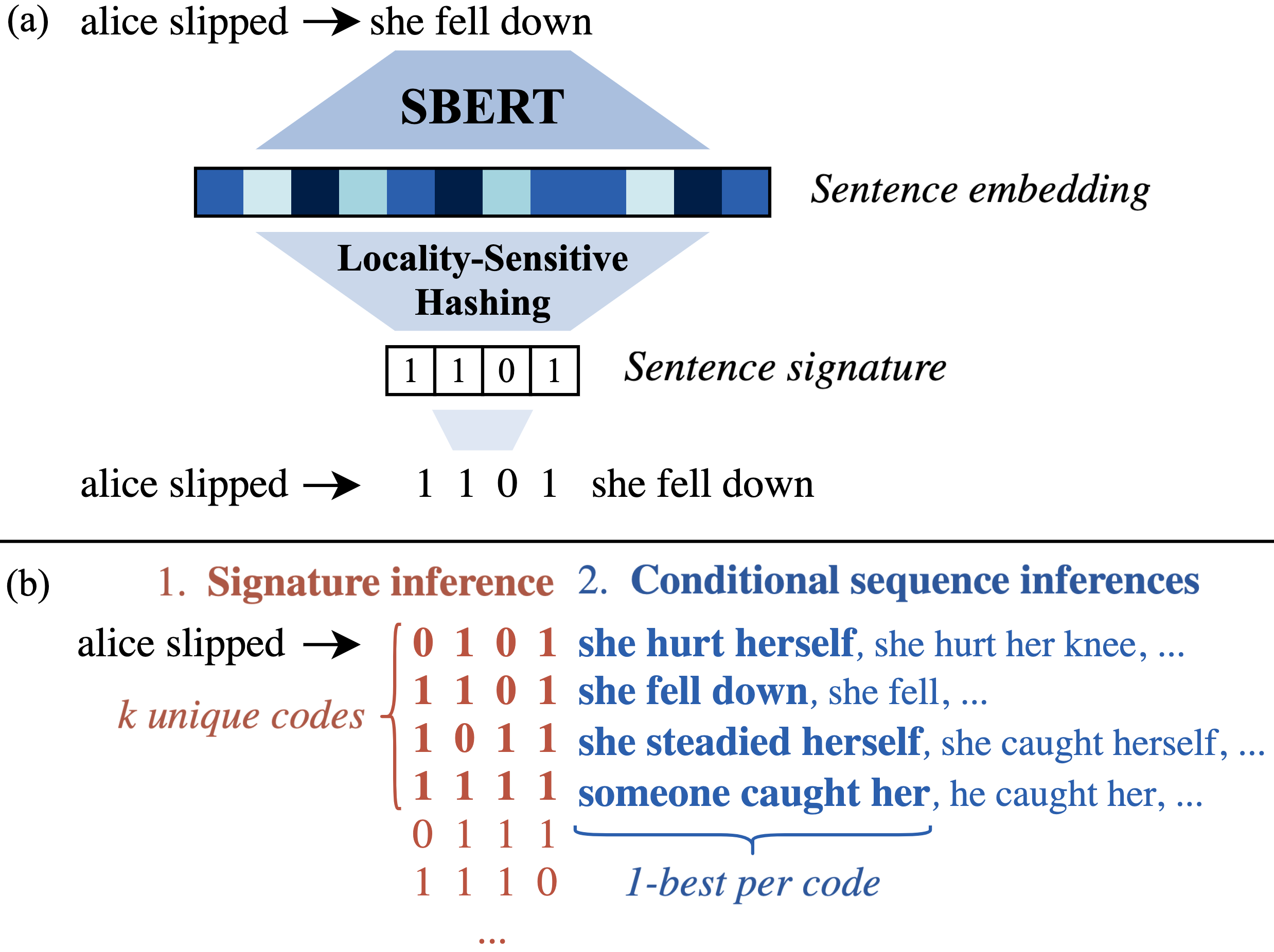
Figure 1: Overview of the cod3s method. In training (a), the target side is prefixed with a discrete signature computed using locality-sensitive hashing (LSH) of the target’s SBERT embedding. At inference (b), a beam search is conditioned on each of $k$ decoded signatures.

Recent methods for improved diversity generation make slight modifications to the neural architecture or beam search algorithm Xu et al. (2018); Li et al. (2016b), or impose lexical constraints during decoding Post and Vilar (2018); Hu et al. (2019a). Shu et al. (2019) propose the use of sentence codes, a technique in which generation is conditioned on a discrete code that aims to induce diversity in syntax or semantics. While their approach is effective for syntactic codes, it is less so for semantics.

In this work, we introduce an improved method for diverse generation conditioned on inferred sentence codes that explicitly capture meaningful semantic differences. We use the contextual sentence embeddings from Sentence-BERT (SBERT; Reimers and Gurevych, 2019), the cosine distances between which correlate highly with human scalar judgments of semantic textual similarity (STS). We construct discrete codes from these embeddings using locality-sensitive hashing Indyk and Motwani (1998); Charikar (2002), producing short binary signatures whose Hamming distances well-preserves the cosine distances between inputs.

Our method induces a bitwise hierarchy of semantic bins whose similarities in signature imply similarities in semantics. Conditioning generation on a signature as a target-side prefix indicates the bin into which the generated sequence falls. We implement a two-stage decoding process that (1) infers the most relevant signatures and (2) decodes sequences via separate prefix-conditioned beams. We term our method cod3s: COnstrained Decoding with Semantic Sentence Signatures.

We demonstrate the effectiveness of cod3s in the context of causal sequence generation Li et al. (2020) through BLEU- and cosine-based diversity measures as well as human evaluation.

2 Related Work

We draw inspiration from recent work in multilingual machine translation (MT) Ha et al. (2016) and domain adaptation Chu and Dabre (2019) in which a language code (e.g. en, de) is prepended to the target to guide generation. Our method for encoding sentence diversity is closely related to MT work by Shu et al. (2019), who condition generation on prefixed sentence codes. They improve the syntactic diversity of sampled translations using codes produced from improved semantic hashing Kaiser and Bengio (2018) with a TreeLSTM-based autoencoder. Their experiments with semantic coding via clustering of BERT Devlin et al. (2019) and FastText Bojanowski et al. (2017) embeddings lead to negligible or negative effects. Outside of MT, Keskar et al. (2019) in a similar vein condition on manually categorized “control codes” that specify style and content, and Mallinson and Lapata (2019) condition on annotated syntactic or lexical change markers that can be learnt from data. We refer readers to Ippolito et al. (2019) for an overview of diverse decoding methods. Few to our knowledge explicitly and effectively encode open-domain semantic diversity.

Text-based causal knowledge acquisition is a well-studied challenge in NLP Radinsky et al. (2012). Recent efforts have investigated open ended causal generation using neural models Bosselut et al. (2019); Li et al. (2020). The latter train a conditional generation model to propose cause or effect statements for a given proposition. The model is trained on the co-released corpus CausalBank, which comprises causal statements harvested from English Common Crawl Buck et al. (2014).

Applications of LSH Indyk and Motwani (1998); Charikar (2002) in NLP began with Ravichandran et al. (2005) who demonstrated its use in fast lexical similarity comparison; later, Van Durme and Lall (2010) showed such hashing could be performed online. More similar to our use case, Petrović et al. (2010) binned tweets via LSH to enable fast first story detection. Most related to ours is work by Guu et al. (2018), who describe a generative sentence model that edits a ‘prototype’ sentence using lexically similar ones retrieved via LSH.

3 cod3s Approach

Our signature construction method, depicted in Figure 1(a), produces a sequence of bits that collectively imply a highly specific bin of sentences with similar semantic meaning. This is accomplished by encoding sentences into high-dimensional vectors that encode degrees of semantic difference and then discretizing the vectors in a way that approximately preserves the difference.

Semantic Embedding Model

We embed a sentence using the contextual encoder Sentence-BERT  (SBERT; Reimers and Gurevych, 2019), a siamese network trained to produce embeddings whose cosine similarity approximates the semantic textual similarity (STS) of the underlying sentences. We select this single sentence encoder over other popular encoders, e.g. BERT, which best encode concatenations of pairs of sentences and therefore do not produce individual embeddings that encode semantic difference retrievable under vector similarity metrics Reimers and Gurevych (2019); Shu et al. (2019). The cosine similarity of embeddings from SRoBERTa-L, the instance of SBERT that we use as our cod3s encoder, has a Spearman $\rho$ correlation of $.863$ with human STS judgements from STSbenchmark Cer et al. (2017). We provide a list of cosine/STS correlations using other models in Appendix E.

Discretization via LSH

Locality-sensitive hashing (LSH; Indyk and Motwani, 1998) maps high-dimensional vectors into low-dimensional sketches for quick and accurate similarity comparison under measures such as cosine or Euclidean distance. We use the popular variant by Charikar (2002), which computes a discrete $b$-bit signature $\texttt{LSH}(\vec{v})=[\texttt{LSH}_{1}(\vec{v}),\dots\texttt{LSH}_{b}(\vec{v})]$. Appendix A provides an overview of this approach. The Hamming distance between two LSH signatures approximates the cosine distance of the underyling vectors:

This approximation degrades with coarser-grained signatures, as shown by the drop in STS correlation in Table 1 (right columns) for LSH with fewer bits.

A Hierarchy of Signatures

Using LSH on SBERT embeddings whose cosine similarity correlates highly with STS induces a hierarchy of semantic bins; the $i+1$th bit partitions each of a set of $i$-bit bins in two. Bins whose signatures differ by few bits have higher semantic overlap, and as the bitwise distance between two signatures increases, so does the difference in meaning of the underlying sentences. Sentences that hash to the same bin—particularly for longer signatures—have very high SBERT cosine similarity and are thus likely semantically homogeneous.

	Cosine	$b$-Bit LSH Hamming Distance
	1024D	256b	128b	32b	16b	8b
STS $\rho$	.863	.845	.828	.742	.652	.549

Table 1: Correlation of SRoBERTa-L embedding cosine distance and LSH Hamming distance with STS judgements from STSBenchmark.

Diverse Decoding Using Signatures

Given source and target sentences $x,y$, we compute the $b$-bit signature $s^{y}=\texttt{LSH}(\texttt{SBERT}(y))$. We then train a model to decode the concatenated sequence $[s^{y}\ y]$, with the $s^{y}$ treated as a $b$-length sequence of individual $0/1$ tokens. At inference time, we decompose the typical conditional decision problem $\hat{y}=\mathop{\text{argmax}}_{y}\{\log p(y\mid x)\}$ into two steps:

As previous work associates the strength of a causal relationship with pointwise mutual information (PMI) Gordon et al. (2012), we modify our objective to maximize the MI between $x$ and each of $s$ and $y$; we adapt the MMI-bidi objective from Li et al. (2016a):

$$\vspace{-0.4em}\hat{s} =\mathop{argmax}_{s}\{\log{p(s\mid x)}+\lambda_{s}\log{p(x\mid s)}\}$$ (1)

$$\hat{y} =\mathop{argmax}_{y}\{\log{p(y\mid x,\hat{s})}+\lambda_{y}\log{p(x\mid y)}\}\vspace{-0.4em}$$ (2)

As shown in Figure 1(b), we first decode the $k$-best distinct sentence codes $\hat{s}_{1},\dots\hat{s}_{k}$ as in Eq. 1. We then perform $k$ conditional inferences in Eq. 2; we take the 1-best sentence from each to produce $\hat{y}_{1},\dots\hat{y}_{k}$. For both signature and sentence decoding, we follow Li et al. and sample an $n$-best list from the forward score $\log{p(s\mid x)}$ (resp. $\log{p(y\mid x,\hat{s}})$) before re-ranking with the added $\lambda$-weighted backward score. We approximate the forward scores using length-normalized beam search with beam size 100 for signatures and 40 for sentences. While $\log{p(s\mid x)}$ and $\log{p(y\mid x,s)}$ can be scored using a single forward model, we find it beneficial to train two, so that the first only learns to score signatures.

Hamming Distance Threshold

As sentences whose signatures differ by few bits show to have highly similar semantics, we impose a threshold heuristic for decoded signatures $\hat{s}_{1},\dots,\hat{s}_{k}$: $\min_{i\neq j}{D(\hat{s}_{i},\hat{s}_{j})}>t$, where $D(\cdot)$ is Hamming distance. We enforce this using a greedy algorithm that considers higher-scoring signatures first, keeping those that satisfy the threshold given the currently kept set and removing those that violate it.

Taken as a whole, our decoding approach aims to generate the single highest-scoring applicable response that falls in each of the N-best inferred sufficiently different semantic bins. The threshold parameter thus provides a way to effectively tune the model to a desired level of semantic diversity.

4 Experiments

We apply cod3s to the task of open-ended causal generation for free-form textual inputs as considered by Li et al. (2020). Given an input statement, the model must suggest a diverse set of possible causes or effects. We train models on sentence pairs from Li et al.’s released dataset, CausalBank, which is scraped from Common Crawl using templatic causal patterns. Following their work, we use 10 million sentence pairs that match the patterns “X, so Y” to train cause-to-effect models and “X because Y” for effect-to-cause models.

We experiment with 16-bit LSH signatures of SBERT embeddings. After prepending target-side bit signatures, pairs are encoded with byte-pair encoding (BPE; Sennrich et al., 2016) using a vocabulary size of 10K. We train Transformer models Vaswani et al. (2017) using the fairseq library Ott et al. (2019). Appendix B provides details for reproducibility.

Evaluation

We show that cod3s induces sensible inference of diverse but relevant semantic bins and causal statements. Examples of generation are shown in Table 3 and additionally Appendix C.

COPA		C $\rightarrow$ E	E $\rightarrow$ C
3-Sets		BL-1 / BL-2 / SB	BL-1 / BL-2 / SB
Baselines
S2S		50.9 / 61.2 / .397	58.1 / 71.4 / .464
S2S + Sigs		46.7 / 58.5 / .323	50.7 / 65.3 / .326
Other Decoding Methods
DPC (Li et al.)		49.2 / 58.1 / .389	57.4 / 67.0 / .425
S2S-RS (Li et al.)		78.2 / 90.3 / .635	75.4 / 89.7 / .632
S2S-RS		83.6 / 95.7 / .735	78.5 / 91.3 / .639
Two-Step cod3s Inferences
Sig	Sent
Beam	Beam	79.1 / 93.2 / .618	70.6 / 84.8 / .625
Beam	MMI	77.0 / 91.9 / .634	72.2 / 85.0 / .613
MMI	MMI	73.6 / 87.9 / .608	72.0 / 85.3 / .586
MMI	MMI-RS	84.2 / 97.1 / .657	76.6 / 89.4 / .617
$-$ Ham Heur		81.1 / 93.9 / .620	70.4 / 84.2 / .508

Cos Threshold:	0	.1	.25	.5	.75
S2S	10.0	6.40	4.52	2.85	1.70
S2S + RS	10.0	9.99	9.86	7.93	3.47
cod3s +MMI +RS	10.0	9.89	9.44	6.55	2.54

Table 2: (Upper) Diversity metrics (BLEU-1 / BLEU-2 / SBERT) over 3-best decoded outputs. (Lower) Count of semantically distinct effect outputs out of 10, with duplicates ruled out using SBERT cosine.

We quantitatively compare cod3s against the outputs of regular seq2seq beam search, as well as of lexically constrained decoding with disjunctive positive constraints (DPC) and random sample decoding (S2S-RS) provided by Li et al. We included in the comparison instances of cod3s with and without MMI reranking, as well as with random sampling in place of beam search.

Automatic Diversity Metrics

We use the formula of Shu et al. (2019), which takes the pairwise average of dissimilarity score $\Delta$ over output set $Y$.

$$\text{Diversity}(Y)=\dfrac{1}{|Y|(|Y|-1)}\sum_{\begin{subarray}{c}y,y^{\prime}\in Y;\ y\neq y^{\prime}\end{subarray}}\Delta(y,y^{\prime})\vspace{-0.3em}$$

To measure lexical diversity, we set $\Delta(y,y^{\prime})$ to be the sentences’ inverse ($100$ minus) BLEU-1 and -2 scores. To measure semantic diversity, we set $\Delta$ to be the cosine distance between their SBERT embeddings. Higher scores imply greater diversity. Following Li et al., we evaluate on 100 examples from an out-of-distribution dev split of the Choice of Plausible Alternatives dataset (COPA; Gordon et al., 2012), with results shown in Table 2. In both cases, cod3s outperforms all other methods except random sampling, the addition of which also improves the diversity of cod3s itself. We also use the SBERT diversity score to count semantically diverse outputs by marking as duplicates those for which the embedding of the completed phrase (“X $\dots$ Y”) falls below some distance threshold from that of an earlier candidate. Table 2 (lower) shows that both the best cod3s model as well as random sampling produce far more semantically distinct statements than the beam search baseline.

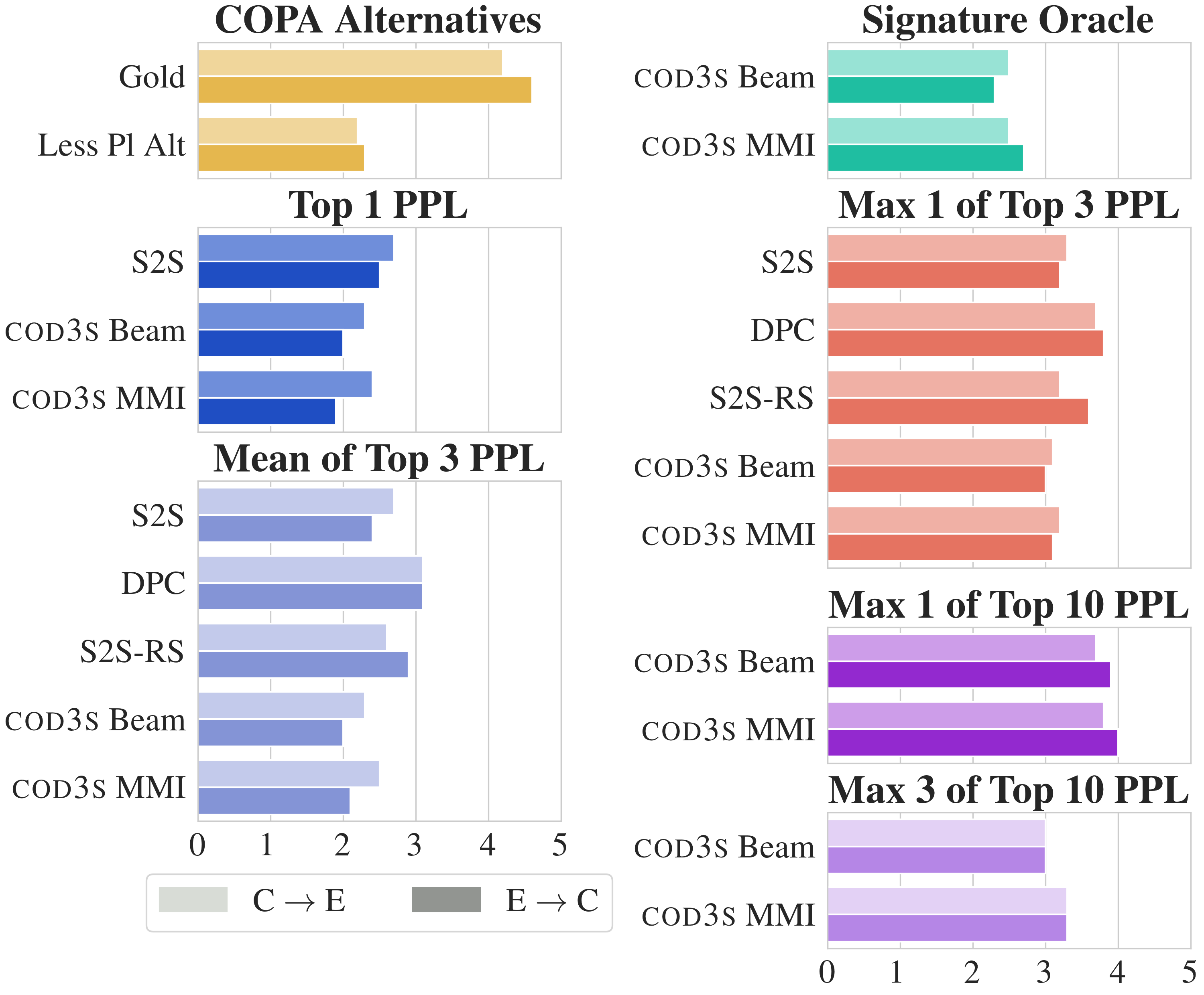
Figure 2: Results of human evaluation of plausibility. Ratings are shown in comparison to the gold answer and less plausible alternative from COPA. Mean/max ratings per input are presented for $1,3$-best outputs ranked by forward score (PPL). To demonstrate that cod3s produces plausible response from many semantic bins, we also show max ratings from top-10 outputs.

Cause Input: my favorite song came on the radio
Bin Medoid	I will try this version for sure	I was quite excited to finally experience it
Ranked Predictions	I decided to listen to it	I was excited to hear it again
	I decided to hear it	I was pleasantly surprised to hear it
	I figured I’d try it	I’m glad to see it here
Effect Input: the executive decided not to hire the applicant
Bin Medoid	I knew that they expected it	they are what earn you cash
Ranked Predictions	they knew she was not qualified	they could not afford the payments
	they knew it would be a mistake	it would cost them money
	she knew she had to	she was paid

Table 3: Examples of generation conditioned on semantic bins. Predictions are ranked according to maximum mutual information (MMI) and shown aside the given bin’s representative medoid.

Human Evaluation

Our automatic metrics quantify diversity without tracking task effectiveness, which we evaluate by collecing judgments on Amazon Mechanical Turk. We ask workers to judge the plausibility of responses as causal completions (on a 0-5 Likert scale). For all methods except cod3s, we use the exact outputs evaluated in Li et al. (2020) and provided to us by the authors. The response sets for these models contain the top 3 decoded sentences under perplexity (PPL). We compare these to the top 3 as well as the top 10 sentences decoded by cod3s with and without MMI re-ranking (signature and sentence, no random sampling) ordered by PPL of the signature tokens. This discrepancy in per-model outputs reflects that we seek to evaluate cod3s, which is specifically crafted to produce a large set of distinct viable candidates, as directly as possible against the Li et al. (2020) responses from models that are not necessarily crafted with the identical aim. Naturally occurring propositions have far more than 10 plausible and distinct causes and effects, and so we would hope that the $10^{\text{th}}$ output of our one-to-many model would have similar quality to the $1^{\text{st}}$ of the other models.

Results are shown in Figure 2. We observe that top 1 and 3 cod3s responses according to PPL (blue) are comparable albeit slightly lower on average than those of the other models. This may partially be attributed to the difficulty of the signature inference step, in which the differences in the top 100 predicted binary sequence PPLs are typically small. A cod3s ‘oracle’ that conditions generation on the gold answer’s signature (which often has low predicted likelihood) performs more competitively (green).

We find that at least 1 of the top 3 signatures predicted by cod3s yields a competitively plausible sentence; when we take the highest plausibility score from the top 3 of each model under their respective PPL orderings (red), cod3s and baseline S2S to be interchangeable. If we expand to the larger set of 10 outputs for cod3s models, we find that the mean of the 3 highest plausibility scores (faded purple) for the MMI model is comparable to the 1 best of the base seq2seq (red) and better than the mean of the top 3 PPL (faded blue) for any model. This indicates that the 10 output set, which shows under automatic metrics to contain higher numbers of semantically diverse statements, also contains at worst a set of 3 outputs that are better than the 3 from models not designed for one-to-many diverse prediction.

Qualitative Analysis

Table 3 shows examples of models predicting and re-ranking sentences within inferred signature bins. Candidate predictions listed in order of MMI score reflect the ability of MMI-based reranking to select the candidates within a bin that are most relevant to the input. Outputs are shown beneath a representative bin medoid, i.e. the sentence with minimized embedding cosine distance from all other training sentences that fall in the bin. The two-step inference process depicted here allows for a level of interpretability on the signature level, as sampling training sentences from the inferred semantic bin gives a snapshot of an inferred semantic space that can be more informative than individual sentences alone.

Future work might explore alternative methods for signature inference. The bit sequence likelihoods predicted by cod3s are often clumped together and/or biased towards signatures that intuitively do not apply to an input but are over-represented in the training set. We also observe that although MMI decoding discourages bland context insensitive statements, there is still a model tendency towards a small set of generic predicates, e.g. ‘having,’ ‘knowing,’ or ‘being able to.’

5 Conclusion

We have outlined cod3s, a method for producing semantically diverse statements in open-ended generation tasks. We design sentence LSH signatures that encode bitwise the semantic similarity of underlying statements; conditioning generation on different signatures yields outputs that are semantically heterogeneous. cod3s leads to more diverse outputs in a multi-target generation task in a controllable and interpretable manner, suggesting the potential of semantically guided diverse decoding for a variety of text generation tasks in the future.

6 Acknowledgments

We thank the reviewers for their insightful comments. We additionally thank Elizabeth Salesky, Huda Khayrallah, Rachel Wicks and Patrick Xia for their discussions, feedback and compute. This work was supported in part by DARPA KAIROS (FA8750-19-2-0034). The views and conclusions contained in this work are those of the authors and should not be interpreted as representing official policies or endorsements by DARPA or the U.S. Government.

Appendix A Random Hyperplane LSH Details

The popular LSH variant introduced by Charikar (2002) leverages random hyperplane projections to compute discrete $b$-length bit signatures. Each individual bit is determined from the sign of the dot product between a given embedding and one of a set of $b$ pre-computed random normal vectors. One geometric intuition is that the hyperplane implied by each random normal vector partitions the full embedding space in half, and the sign of the dot product designates the partition into which the input embedding falls. This is illustrated in Figure 3 using a simplified case with a 2-D vector $v$ and three random vectors $r_{1},r_{2},r_{3}$ indicating partitions of the Cartesian plane.

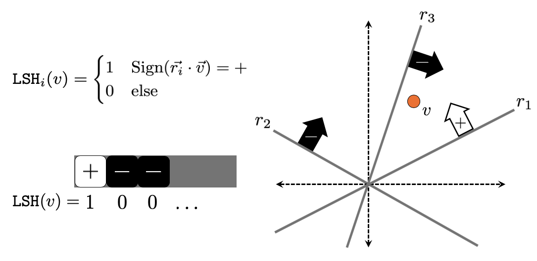
Figure 3: Computation of a 2D vector $v$’s LSH bit signature as the signs of the dot products with $d$ random normal vectors $r_{1},\dots,r_{b}$.

Formally, given a set of high-dimensional vectors in $\mathbbm{R}^{D}$, we randomly sample $b\ll D$ random vectors $\vec{r}_{1},\dots\vec{r}_{d}$ from the $D-$dimensional Gaussian distribution. Then, given a high-dimensional embedding $\vec{v}$, we construct the $b$-bit signature $\texttt{LSH}(v)=[\texttt{LSH}_{1}(v),\dots\texttt{LSH}_{d}(v)]$ using the hash functions

$$\texttt{LSH}_{i}(v)=\begin{cases}1&\text{if }\vec{r_{i}}\cdot\vec{v}\geq 0\\ 0&\text{if }\vec{r_{i}}\cdot\vec{v}<0\end{cases}$$

The number of matching bits in the signatures of two vectors $u,v$ provides an estimate of their hash collision probability, i.e. the likelihood that they fall in the same partition of any random hyperplane. This probability is provably monotonically increasing with the vectors’ inner product. Goemans and Williamson (1995) similarly prove that the Hamming distance between signatures is proportional to the angle between the vectors, which correlates highly with cosine distance barring high discrepancies in vector norms.

Appendix B Training Details

fairseq-train
 --adam-betas "(0.9, 0.98)"
 --arch transformer_iwslt_de_en
 --criterion
   label_smoothed_cross_entropy
 --label-smoothing 0.1
 --dropout 0.1 --weight-decay 0
 --bpe sentencepiece
 --optimizer adam  --clip-norm 0.1
 --lr 5e-4 --lr-scheduler inverse_sqrt
 --warmup-updates 4000
 --max-epoch 10
 --share-all-embeddings

We train models with fairseq using the transformer_iwslt_de_en architecture. We use 6 encoder and decoder layers with 512-dimensional hidden states and shared embedding layers (a total of 36.6M trainable parameters). Signature tokens are assigned special tokens during BPE encoding. We train models for 10 epochs with an early stopping patience of 2 validations. We use the Adam optimizer Kingma and Ba (2015) with $0.1$-smoothed cross entropy loss, a $510-4$ learning rate with inverser square root scheduling, $0.1$ dropout and $0.1$ norm clipping. All other training parameters were the fairseq defaults at the time of submission. We observe performance drops when 1) norm clipping threshold is not sufficiently low, 2) BPE vocabulary size is 32K instead of 10K, and 3) weight decay is set to .001. Training takes roughly 12 hours on two Titan 24GB RTX GPUs for each of four models (two forward, two backward for MMI reranking).

Backwards scoring models for MMI-bidi are trained with the opposite dataset as their corresponding forward models; we find training most effective when the data’s syntactic direction (“X …Y”) matches the direction of inference (X $\rightarrow$ Y). In other words, all C$\rightarrow$ E models are trained on “X, so Y” data regardless of their use as forward or backward scoring models. We used the “X because Y” training split from Li et al. (2020). We constructed the 10M “X so Y” examples ourselves: we took a 20M random sample of all such examples in the dataset, filtered to remove sentences a) containing numerical and special characters or b) containing either a source or target with greater than 12 tokens, and then downsampled the remaining set to a 10M/4K/4K train/dev/test split.

Causalbank		C $\rightarrow$ E	E $\rightarrow$ C
3-Sets		BL-1 / BL-2 / SB	BL-1 / BL-2 / SB
Baselines
S2S		54.2 / 62.9 / .348	59.8 / 71.4 / .428
S2S + Sigs		47.5 / 56.6 / .248	56.2 / 70.3 / .302
Other Decoding Methods
DPC (Li et al.)		41.8 / 49.4 / .293	47.4 / 55.3 / .319
S2S-RS (Li et al.)		77.5 / 89.3 / .567	82.6 / 94.1 / .622
S2S-RS		87.0 / 96.8 / .676	82.1 / 92.1 / .626
Two-Step cod3s Inferences
Sig	Sent
Beam	Beam	84.0 / 94.2 / .603	77.1 / 89.6 / .558
Beam	MMI	80.0 / 90.9 / .571	74.0 / 86.3 / .542
MMI	MMI	75.1 / 86.6 / .554	70.7 / 83.9 / .543
MMI	MMI-RS	85.9 / 95.4 / .620	78.1 / 90.9 / .563
$-$ Ham Heur		80.4 / 90.8 / .521	74.0 / 87.8 / .501
COPA		C $\rightarrow$ E	E $\rightarrow$ C
10-Sets		BL-1 / BL-2 / SB	BL-1 / BL-2 / SB
Baselines
S2S		59.9 / 71.5 / .466	62.5 / 76.7 / .509
S2S + Sigs		52.4 / 64.8 / .360	55.3 / 70.0 / .397
S2S-RS		84.7 / 96.9 / .746	83.8 / 95.1 / .693
Two-Step cod3s Inferences
Sig	Sent
Beam	Beam	81.7 / 95.5 / .658	75.8 / 89.6 / .660
Beam	MMI	78.5 / 93.1 / .653	75.1 / 89.2 / .639
MMI	MMI	75.8 / 90.6 / .633	74.3 / 88.2 / .612
MMI	MMI-RS	82.6 / 96.1 / .676	78.2 / 91.8 / .647
$-$ Ham Heur		80.5 / 93.8 / .619	72.5 / 86.2 / .544

Table 4: Automatic diversity metrics (1-BLEU / 2-BLEU / SBERT) evaluated over the outputs of 16-bit cod3s and other decoding methods. Results are shown for 3-best outputs over 100 in-distribution CausalBank examples and 10-best over out-of-distribution COPA. Following Li et al. (2020), the same 100 “X because Y” pairs were used to evaluate models of both inference directions.

Appendix C Decoding According to Semantic Bins

We experimented with bit lengths of 8, 16, and 32, and found the middle value to best balance specificity with accuracy. We also explored a variant that merged signatures into a single token rather than treating them as token-per-bit, but found the model to perform qualitatively worse. We experimented with Hamming distance heuristic thresholds of 0 through 6 and found the best value (2) for 16-bit cod3s using qualitative analysis of side-by-side predictions. The MMI-bidi $\lambda_{s},\lambda_{y}$ values were found using simple grid search, comparison of automatic metrics, and side-by-side analysis. The nature of the output set is sensitive to only large changes (orders of magnitude) in $\lambda_{s}$ values, as the likelihoods of signature sequences are rather close in value; however, smaller, 0.1-increment changes to the sentence weight $\lambda_{y}$ showed to have a greater effect on the relevance and specificity of output causes/effects. This comports with results from previous applications of MMI-bidi decoding for sentences Li et al. (2016a).

Table 7 shows side-by-side outputs of models with and without MMI re-ranking conditioned on the same n-best inferred signatures. Table 4 shows results of automatic diversity evaluation on the in-distribution training sample from CausalBank following Li et al. (2020). Table 5 provides a tabular version of the human plausibility scores depicted in Figure 2.

C $\rightarrow$ E / E $\rightarrow$ C    Gold: 4.2 / 4.6			Pl Alt: 2.2 / 2.3
	Top PPL		Max Score
Method	T1	T3	T1	T3 (/ 10)
S2S	2.7 / 2.5	2.7 / 2.4	3.3 / 3.2
DPC	—	3.1 / 3.1	3.7 / 3.8
S2S-RS	—	2.6 / 2.9	3.2 / 3.6
cod3s
Beam	2.3 / 2.0	2.3 / 2.0	3.1 / 3.0
(Oracle)	2.5 / 2.3
(10 Outputs)			3.7 / 3.9	3.0 / 3.0
MMI	2.4 / 1.9	2.5 / 2.1	3.2 / 3.1
(Oracle)	2.5 / 2.7
(10 Outputs)			3.8 / 4.0	3.3 / 3.3

Table 5: Tabular form of human evaluation results displayed in Figure 2.

Cause: the tenant misplaced his keys to his apartment			Effect: the man threw out the bread
1	he couldn’t leave the house		1	he didn’t want to eat it
2	he couldn’t get out of the house	Dupl. of 1 (.01)	2	he didn’t like it
3	he had to get a new one		3	he didn’t like the taste	Dupl. of 2 (.05)
4	he had to go back to the hotel		4	it was too much for him to handle
5	he had to find a new one	Dupl. of 3 (.02)	5	he didn’t want to cook it	Dupl. of 1 (.07)
6	he couldn’t get into the house	Dupl. of 1 (.06)	6	he didn’t know how to cook it
7	he had to go back to the house		7	it wasn’t good for him	Dupl. of 1 (.07)
8	he couldn’t leave the building	Dupl. of 1 (.02)	8	he didn’t like how it tasted	Dupl. of 2 (.05)
9	he had to go to the police station		9	he couldn’t eat it	Dupl. of 1 (.06)
10	he had to go back to his apartment	Dupl. of 7 (.07)	10	it was overcooked

Table 6: Detection of duplicate causes and effects using a threshold SBERT embedding cosine distance of $0.1$. We embed the full “X …Y” statements so as to provide context to the paraphrase detection. Model outputs are those of a regular seq2seq.

Appendix D Counting Semantically Distinct Outputs using SBERT

We construct a method for automatically counting the number of semantically diverse sentences in a candidate cause/effect set. We encode each prediction with the context of the input by taking the SBERT embedding of the completed sentence ”X {because, so} Y.” We then rule out all sentences whose embedding cosine distance from that of a higher-ranked candidate is lower than some threshold. We use a simple grid search over various threshold values and find that a value of $.1$ yields a sensitivity to paraphrastic cause/effect predictions similar to that of a human reader. As other tasks might merit different such thresholds, we provide multiple such counts in Table 2. Table 6 shows example cases of duplicate detection among generated candidate sets.

Appendix E Cosine/LSH Hamming Correlations with STS and Bin Statistics

Table 8 shows the Spearman $\rho$ coefficient with STSbenchmark judgments for cosine and approximate LSH Hamming distances of embeddings for BERT, SBERT (and larger variant SRoBERTa), and pBERT Hu et al. (2019b), a BERT model fine-tuned to predict paraphrastic similarity, albiet not via angular similarity of embeddings. Table 9 provides details regarding the distributions of sentences into LSH bins of differing levels of granularity using SRoBERTa-L embeddings.

Appendix F Human Evaluation of Plausibility

We showed 200 COPA input statements (100 each for cause-to-effect and effect-to-cause) to Amazon Mechanical Turk workers and asked them to judge the plausibility of model predictions, specifically as completions of a causal statement of the form “X because Y” or “Y, so X.” The order of the examples were randomized. Four annotators rated each input/prediction pair. We required annotators to have at least a 97% approval rating, be located in the US, and have completed at least 500 HITs. Annotators were given an hour to complete each HIT. The median completion time for the task was 5 minutes, and workers were paid $0.50 per HIT. We included at least two attention checks.

W/O MMI Reranking	W/ MMI Reranking	Conditioned Bin Medoid
Cause: I was confused by the professor’s lecture
Gold Effect: I asked the professor questions
I asked him about it	I asked a few questions	I need some feedback from you (Gold bin)
I decided to try it	I decided to look it up	I will try this version
I thought I’d ask here	I decided to ask the teacher	I might change them at some point
I decided to open it up	I opened it up and started reading	you can check it out
I did my own research	I did a quick math lesson	it is easy to get everything aligned
Cause: several witnesses of the crime testified against the suspect
Gold Effect: the suspect was convicted
he’s got that going for him	the case was taken to court	we did it this way (Gold bin)
he knew what to do	the case was resolved	this is a simple solution that makes sense
the jury is still out	the jury was left to investigate	everyone will know what it is
they didn’t have to deal with it	there was no need for an attorney	I guess I won’t have to think about this
it was easy to follow	the police proceeded to investigate	this recipe is ready to go
Cause: the papers were disorganized
Gold Effect: I put them into alphabetical order
I had to enter them	I had to print them out	the opening sequence was there (Gold bin)
that’s out of the question	I gave up on it	I won’t use it in anything anymore
I decided to skip it	I decided not to publish them	I opted not to do any
I got a new one	I had to edit them	we came at a good time
we had to start all over again	I had to start all over again	it should be open by then
Effect: the woman hired a lawyer
Gold Cause: she decided to sue her employer
she wanted to	she wanted a lawyer	they want to crack down on it (Gold bin)
she thought she could win	she wanted to be in charge of her case	it can be an ideal method for you to succeed
she had a plan	she felt she had enough evidence	it was what we had and it turned out fine
she trusted him	she wanted to help people	I did trust and respect the person
she wanted to be a mother	she wanted to protect her family	all ages enjoy them
Effect: I avoided giving a straight answer to the question
Gold Cause: the question made me uncomfortable
I didn’t want to offend anyone	I didn’t want to offend anyone	I didn’t like to speak (Gold bin)
I didn’t understand it	I didnt know what I was talking about	I didn’t understand them
there was no one to talk to	I didn’t want to talk about it	I’m not allowed to talk to them about anything
the answer was obvious	I thought the answer would be obvious	everyone’s familiar with it
I was so embarrassed	I thought I was stupid	it looked ridiculously saturated
Effect: I learned how to play the board game
Gold Cause: my friend explained the rules to me
I learned a lot about the game	I wanted to learn to play the game	it offers some good information (Gold bin)
i felt like it	i felt i had to	I feel it to be so
it was so easy	it was easy to play	it is done nicely and realistically
it worked	i knew i was going to play it	they have now got it right
I love to play online	I wanted to play online	the online wants anyone spreading the phrase

Table 7: Example cod3s output responses with and without MMI-bidi sentence re-ranking. Predictions are shown alongside their conditioned bin’s representative medoid sentence. “Bin oracle” predictions conditioned on the signature of gold sequence (Gold bin) are shown for comparison.

bits	4	8	16	32	64	128	256	full
BERT-B	0.01	0.08	0.11	0.12	0.09	0.14	0.15	0.13
pBERT-B	0.05	0.09	0.09	0.11	0.13	0.14	0.15	0.14
SBERT-B	0.41	0.51	0.61	0.69	0.76	0.80	0.82	0.85
SBERT-L	0.42	0.51	0.64	0.72	0.77	0.80	0.82	0.85
SRoBERTa-B	0.38	0.51	0.61	0.71	0.77	0.81	0.83	0.85
SRoBERTa-L	0.42	0.55	0.65	0.74	0.80	0.83	0.85	0.86

Table 8: Spearman $\rho$ correlation of LSH Hamming-based cosine approximations with human STS judgements on STSBenchmark (as well as cosine similarity of the full 768/1024-dimension embeddings)

LSH Bits	4	8	12	16	20	24	28	32
Distinct Sentences / Populated Bin	5.55e5	3.47e4	2166.97	135.85	10.75	2.47	1.33	1.10
	$\pm$ 1.91e5	$\pm$ 2.37e4	$\pm$ 2671.91	$\pm$ 225.40	$\pm$ 22.32	$\pm$ 4.62	$\pm$ 1.51	$\pm$ 0.72
Distinct Unigrams / Populated Bin	1.28e5	2.15e4	3191.00	415.27	54.42	15.71	9.24	7.87
	$\pm$ 2.24e4	$\pm$ 8446.11	$\pm$ 2378.42	$\pm$ 430.38	$\pm$ 73.41	$\pm$ 19.10	$\pm$ 6.63	$\pm$ 3.64
% Buckets Populated	100	100	100	99.69	78.73	21.45	2.49	0.19
STS $\rho$	0.42	0.55	0.61	0.65	0.69	0.71	0.73	0.74

Table 9: Analysis of bin clusters using the effects of 10 million CausalBank ”X because Y” pairs.

Figure 4: Interface shown to Amazon Mechanical Turk workers during collection of plausibility judgments.

References

- Bojanowski et al. (2017) Piotr Bojanowski, Edouard Grave, Armand Joulin, and Tomas Mikolov. 2017. Enriching word vectors with subword information. Transactions of the Association for Computational Linguistics, 5:135–146.
- Bosselut et al. (2019) Antoine Bosselut, Hannah Rashkin, Maarten Sap, Chaitanya Malaviya, Asli Celikyilmaz, and Yejin Choi. 2019. COMET: Commonsense transformers for automatic knowledge graph construction. In Proceedings of the 57th Annual Meeting of the Association for Computational Linguistics, pages 4762–4779, Florence, Italy. Association for Computational Linguistics.
- Buck et al. (2014) Christian Buck, Kenneth Heafield, and Bas van Ooyen. 2014. N-gram counts and language models from the common crawl. In Proceedings of the Ninth International Conference on Language Resources and Evaluation (LREC-2014), pages 3579–3584, Reykjavik, Iceland. European Languages Resources Association (ELRA).
- Cer et al. (2017) Daniel Cer, Mona Diab, Eneko Agirre, Iñigo Lopez-Gazpio, and Lucia Specia. 2017. SemEval-2017 task 1: Semantic textual similarity multilingual and crosslingual focused evaluation. In Proceedings of the 11th International Workshop on Semantic Evaluation (SemEval-2017), pages 1–14, Vancouver, Canada. Association for Computational Linguistics.
- Charikar (2002) Moses S Charikar. 2002. Similarity estimation techniques from rounding algorithms. In Proceedings of the thiry-fourth annual ACM symposium on Theory of computing, pages 380–388.
- Chu and Dabre (2019) Chenhui Chu and Raj Dabre. 2019. Multilingual multi-domain adaptation approaches for neural machine translation. arXiv preprint arXiv:1906.07978.
- Devlin et al. (2019) Jacob Devlin, Ming-Wei Chang, Kenton Lee, and Kristina Toutanova. 2019. BERT: Pre-training of deep bidirectional transformers for language understanding. In Proceedings of the 2019 Conference of the North American Chapter of the Association for Computational Linguistics: Human Language Technologies, Volume 1 (Long and Short Papers), pages 4171–4186, Minneapolis, Minnesota. Association for Computational Linguistics.
- Goemans and Williamson (1995) Michel X. Goemans and David P. Williamson. 1995. Improved approximation algorithms for maximum cut and satisfiability problems using semidefinite programming. J. ACM, 42(6):1115–1145.
- Gordon et al. (2012) Andrew Gordon, Zornitsa Kozareva, and Melissa Roemmele. 2012. SemEval-2012 task 7: Choice of plausible alternatives: An evaluation of commonsense causal reasoning. In *SEM 2012: The First Joint Conference on Lexical and Computational Semantics – Volume 1: Proceedings of the main conference and the shared task, and Volume 2: Proceedings of the Sixth International Workshop on Semantic Evaluation (SemEval 2012), pages 394–398, Montréal, Canada. Association for Computational Linguistics.
- Guu et al. (2018) Kelvin Guu, Tatsunori B. Hashimoto, Yonatan Oren, and Percy Liang. 2018. Generating sentences by editing prototypes. Transactions of the Association for Computational Linguistics, 6:437–450.
- Ha et al. (2016) Thanh-Le Ha, Jan Niehues, and Alexander Waibel. 2016. Toward multilingual neural machine translation with universal encoder and decoder. International Conference on Spoken Language Translation.
- Hu et al. (2019a) J. Edward Hu, Huda Khayrallah, Ryan Culkin, Patrick Xia, Tongfei Chen, Matt Post, and Benjamin Van Durme. 2019a. Improved lexically constrained decoding for translation and monolingual rewriting. In Proceedings of the 2019 Conference of the North American Chapter of the Association for Computational Linguistics: Human Language Technologies, Volume 1 (Long and Short Papers), pages 839–850, Minneapolis, Minnesota. Association for Computational Linguistics.
- Hu et al. (2019b) J Edward Hu, Abhinav Singh, Nils Holzenberger, Matt Post, and Benjamin Van Durme. 2019b. Large-scale, diverse, paraphrastic bitexts via sampling and clustering. In Proceedings of the 23rd Conference on Computational Natural Language Learning (CoNLL), pages 44–54.
- Indyk and Motwani (1998) Piotr Indyk and Rajeev Motwani. 1998. Approximate nearest neighbors: Towards removing the curse of dimensionality. In Proceedings of the Thirtieth Annual ACM Symposium on Theory of Computing, STOC ’98, page 604–613, New York, NY, USA. Association for Computing Machinery.
- Ippolito et al. (2019) Daphne Ippolito, Reno Kriz, Joao Sedoc, Maria Kustikova, and Chris Callison-Burch. 2019. Comparison of diverse decoding methods from conditional language models. In Proceedings of the 57th Annual Meeting of the Association for Computational Linguistics, pages 3752–3762, Florence, Italy. Association for Computational Linguistics.
- Kaiser and Bengio (2018) Łukasz Kaiser and Samy Bengio. 2018. Discrete autoencoders for sequence models. arXiv preprint arXiv:1801.09797.
- Keskar et al. (2019) Nitish Shirish Keskar, Bryan McCann, Lav R Varshney, Caiming Xiong, and Richard Socher. 2019. CTRL: A conditional transformer language model for controllable generation. arXiv preprint arXiv:1909.05858.
- Kingma and Ba (2015) Diederik P. Kingma and Jimmy Ba. 2015. Adam: A method for stochastic optimization. In 3rd International Conference on Learning Representations, ICLR 2015, San Diego, CA, USA, May 7-9, 2015, Conference Track Proceedings.
- Li et al. (2016a) Jiwei Li, Michel Galley, Chris Brockett, Jianfeng Gao, and Bill Dolan. 2016a. A diversity-promoting objective function for neural conversation models. In Proceedings of the 2016 Conference of the North American Chapter of the Association for Computational Linguistics: Human Language Technologies, pages 110–119, San Diego, California. Association for Computational Linguistics.
- Li et al. (2016b) Jiwei Li, Will Monroe, and Dan Jurafsky. 2016b. A simple, fast diverse decoding algorithm for neural generation. arXiv preprint arXiv:1611.08562.
- Li et al. (2013) Ping Li, Michael Mitzenmacher, and Anshumali Shrivastava. 2013. Coding for random projections. In International Conference on Machine Learning, pages 676–684.
- Li et al. (2020) Zhongyang Li, Xiao Ding, Ting Liu, J. Edward Hu, and Benjamin Van Durme. 2020. Guided generation of cause and effect. IJCAI.
- Mallinson and Lapata (2019) Jonathan Mallinson and Mirella Lapata. 2019. Controllable sentence simplification: Employing syntactic and lexical constraints. arXiv preprint arXiv:1910.04387.
- Ott et al. (2019) Myle Ott, Sergey Edunov, Alexei Baevski, Angela Fan, Sam Gross, Nathan Ng, David Grangier, and Michael Auli. 2019. fairseq: A fast, extensible toolkit for sequence modeling. In Proceedings of NAACL-HLT 2019: Demonstrations.
- Petrović et al. (2010) Saša Petrović, Miles Osborne, and Victor Lavrenko. 2010. Streaming first story detection with application to twitter. In Human Language Technologies: The 2010 Annual Conference of the North American Chapter of the Association for Computational Linguistics, pages 181–189, Los Angeles, California. Association for Computational Linguistics.
- Post (2018) Matt Post. 2018. A call for clarity in reporting BLEU scores. In Proceedings of the Third Conference on Machine Translation: Research Papers, pages 186–191, Belgium, Brussels. Association for Computational Linguistics.
- Post and Vilar (2018) Matt Post and David Vilar. 2018. Fast lexically constrained decoding with dynamic beam allocation for neural machine translation. In Proceedings of the 2018 Conference of the North American Chapter of the Association for Computational Linguistics: Human Language Technologies, Volume 1 (Long Papers), pages 1314–1324, New Orleans, Louisiana. Association for Computational Linguistics.
- Radinsky et al. (2012) Kira Radinsky, Sagie Davidovich, and Shaul Markovitch. 2012. Learning causality for news events prediction. In Proceedings of the 21st international conference on World Wide Web, pages 909–918.
- Ravichandran et al. (2005) Deepak Ravichandran, Patrick Pantel, and Eduard Hovy. 2005. Randomized algorithms and NLP: Using locality sensitive hash functions for high speed noun clustering. In Proceedings of the 43rd Annual Meeting of the Association for Computational Linguistics (ACL’05), pages 622–629, Ann Arbor, Michigan. Association for Computational Linguistics.
- Reimers and Gurevych (2019) Nils Reimers and Iryna Gurevych. 2019. Sentence-bert: Sentence embeddings using siamese bert-networks. In Proceedings of the 2019 Conference on Empirical Methods in Natural Language Processing. Association for Computational Linguistics.
- Sennrich et al. (2016) Rico Sennrich, Barry Haddow, and Alexandra Birch. 2016. Neural machine translation of rare words with subword units. In Proceedings of the 54th Annual Meeting of the Association for Computational Linguistics (Volume 1: Long Papers), pages 1715–1725, Berlin, Germany. Association for Computational Linguistics.
- Shu et al. (2019) Raphael Shu, Hideki Nakayama, and Kyunghyun Cho. 2019. Generating diverse translations with sentence codes. In Proceedings of the 57th Annual Meeting of the Association for Computational Linguistics, pages 1823–1827, Florence, Italy. Association for Computational Linguistics.
- Van Durme and Lall (2010) Benjamin Van Durme and Ashwin Lall. 2010. Online generation of locality sensitive hash signatures. In Proceedings of the ACL 2010 Conference Short Papers, pages 231–235, Uppsala, Sweden. Association for Computational Linguistics.
- Vaswani et al. (2017) Ashish Vaswani, Noam Shazeer, Niki Parmar, Jakob Uszkoreit, Llion Jones, Aidan N Gomez, Łukasz Kaiser, and Illia Polosukhin. 2017. Attention is all you need. In Advances in neural information processing systems, pages 5998–6008.
- Xu et al. (2018) Qiongkai Xu, Juyan Zhang, Lizhen Qu, Lexing Xie, and Richard Nock. 2018. D-page: Diverse paraphrase generation. ArXiv, abs/1808.04364.