A General Framework for Decentralized Safe Optimal Control of Connected and Automated Vehicles in Multi-Lane Intersections

Abstract

We address the problem of optimally controlling Connected and Automated Vehicles (CAVs) arriving from four multi-lane roads at an intersection where they conflict in terms of safely crossing (including turns) with no collision. The objective is to jointly minimize the travel time and energy consumption of each CAV while ensuring safety. This problem was solved in prior work for single-lane roads. A direct extension to multiple lanes on each road is limited by the computational complexity required to obtain an explicit optimal control solution. Instead, we propose a general framework that first converts a multi-lane intersection problem into a decentralized optimal control problem for each CAV with less conservative safety constraints than prior work. We then employ a method combining optimal control and control barrier functions, which has been shown to efficiently track tractable unconstrained optimal CAV trajectories while also guaranteeing the satisfaction of all constraints. Simulation examples are included to show the effectiveness of the proposed framework under symmetric and asymmetric intersection geometries and different schemes for CAV sequencing.

I INTRODUCTION

Intersections are the main bottlenecks for urban traffic. As reported in [1], congestion in these areas causes US commuters to spend 6.9 billion hours more on the road and to purchase an extra 3.1 billion gallons of fuel, resulting in a substantial economic loss to society. The coordination and control problems at intersections are challenging in terms of safety, traffic efficiency, and energy consumption [1, 2].

The emergence of Connected and Automated Vehicles (CAVs) provides a promising way for better planning and controlling trajectories to reduce congestion and ultimately improve safety as well as efficiency. Enabled by vehicle-to-vehicle (V2V) and vehicle-to-infrastructure (V2I) communication, CAVs can exchange real-time operational data with vehicles in their vicinity and communicate with the infrastructure [3]. Based on these technologies, researchers have made significant progress in the optimal control of CAVs at intersections. One of the prevailing ideas is to formulate an optimization problem whose decision variables are both crossing sequences and control inputs (e.g., desired velocity and desired acceleration). Hult et al. [4] formulated the traffic coordination problem at a three-way intersection as an optimal control problem where it is required that the trajectories of any two vehicles do not intersect in order to guarantee safety. However, it is not explicitly explained how to realize such safety constraints. Some recent studies show that we can realize safety constraints by introducing binary variables to represent crossing sequences, which results in Mixed-Integer Linear Programming (MILP) problems [5]. Though some techniques, such as the grouping scheme [6], have been proposed to accelerate the computation process, it is still difficult to extend this method to multi-lane intersections with a large number of vehicles which may also change lanes along the way. In terms of optimizing control inputs, Model Predictive Control (MPC) is effective for problems with simple (usually linear or linearized) vehicle dynamics and constraints. However, when the vehicle dynamics are highly nonlinear and complex, the whole problem becomes a non-linear MPC whose computation time is still prohibitive for practical applications [7].

Another idea is to decompose the whole optimization problem into two separate problems, i.e., first determining the crossing sequence and then solving for CAV control inputs according to this crossing sequence [8]. The most straightforward crossing sequence mechanism is the First-In-First-Out (FIFO) rule. For example, Dresner and Stone [9] proposed an autonomous intersection management cooperative driving strategy which divides the intersection into grids (resources) and assigns these grids to CAVs in a FIFO manner. In [10] and [11], a decentralized optimal control framework is designed for CAVs to jointly minimize energy and time by deriving the desired CAV arrival times at an intersection based on the FIFO crossing sequence. However, some recent studies have shown that the performance of the FIFO mechanism can lead to poor performance in some cases [12]. In [13], a Dynamic Resequencing (DR) scheme is designed to adjust the crossing sequence whenever a new CAV enters the intersection control zone and showed that this scheme is computationally efficient and improves traffic efficiency. Xu et al. [14] proposed a Monte Carlo Tree Search (MCTS)-based cooperative strategy to find a promising crossing sequence for all CAVs and demonstrated that this strategy may determine a good enough sequence even for complicated multi-lane intersections where the search space is enormous. After determining the crossing sequence, these studies also use the analytical solutions proposed in [10] and [11] to solve for the optimal control inputs. Although [15] has extended this solution to consider speed-dependent rear-end safety constraints, the resulting computational cost significantly increases. Moreover, it is difficult to generalize this optimal control method for complex and nonlinear vehicle dynamics without incurring computational costs which make its real-time applicability prohibitive.

To address the above limitations, we propose an approach which combines the use of Control Barrier Functions (CBFs) with the conventional optimal control method to bridge the gap between optimal control solutions (which represent a lower bound for the optimal achievable cost) and controllers which can provably guarantee on-line safe execution [16]. The key idea is to design CAV trajectories which optimally track analytically tractable solutions of the basic intersection-crossing optimization problem while also provably guaranteeing that all safety constraints are satisfied. Through CBFs, we can map continuously differentiable state constraints into new control-based constraints. Due to the forward invariance of the associated set [17, 18, 19], a control input that satisfies these new constraints is also guaranteed to satisfy the original state constraints. This property makes the CBF method effective even when the vehicle dynamics and constraints become complicated and include noise.

Along these lines, the main contribution of this paper is a novel decentralized optimal control framework combining the optimal control and CBF methods for a multi-lane intersection. Specifically, we first formulate the multi-lane intersection problem as an optimal control problem whose objective is to jointly minimize the traffic delay and energy consumption while guaranteeing that all CAVs safely cross a four-way intersection that includes left and right turns. Unlike prior work, we replace roadway segments referred to as “merging zones” or “conflict zones” by Merging Points (MPs) which are much less conservative while still guaranteeing collision avoidance. Allowing lane-changing behavior, we design a strategy to determine the desirable locations of lane-changing MPs for all CAVs. Then, we propose a search algorithm to quickly determine rear-end safety constraints and lateral safety constraints that every CAV has to meet. Once these constraints are specifed for any CAV, we design an Optimal Control and Barrier Function (OCBF) controller for solving the problem efficiently, as verified through multiple simulation experiments. Our framework can accommodate a variety of resequencing methods for finding a near-optimal crossing sequence, including the aforementioned DR and MCTS schemes, leading to improved performance compared to the FIFO rule, especially when the intersection is geometrically asymmetrical.

The paper is organized as follows. Section II formulates the multi-lane intersection problem as an optimal control problem with safety constraints applied to a sequence of MPs. Section III introduces our search algorithm for determining all safety constraints pertaining to a given CAV, and Section IV presents our joint optimal and control barrier function controller. Section V validates the effectiveness of the proposed method through simulation experiments. Finally, Section VI gives concluding remarks.

II PROBLEM FORMULATION

Figure 1 shows a typical intersection with multiple lanes. The area within the outer red circle is called a Control Zone (CZ), and the length of each CZ segment is $L_{1}$ which is initially assumed to be the same for all entry points to the intersection; extensions to asymmetrical intersections are straightforward and discussed in Section V.D. The significance of the CZ is that it allows all CAVs to share information and be automatically controlled while in it. Red dots show all MPs where potential collisions may occur. We assume that the motion trajectory of each CAV in the intersection is determined upon its entrance to the CZ (see grey lines in Fig. 1). Based on these trajectories, all MPs in the intersection are fixed and can be easily determined. However, unlike prior similar studies, we also allow possible lane-changing behaviors in the CZ, which adds generality to our method. In order to avoid potential collisions with new coming vehicles and to conform with the driving rules that vehicles are prohibited from changing lanes when they are very close to the intersection, these lane changes are only allowed in a “lane-changing zone”, i.e., an area between the two blue lines shown in Fig. 1. We use dotted lines to differentiate these zones from the rest of the area where solid lines are shown. The distance from the entry of the CZ to the lane-changing zone is $L_{2}$ and the length of the lane-changing zone is $L_{3}$. Since we initially consider a symmetrical intersection, $L_{2}$ and $L_{3}$ are the same for all lanes. However, it is easy to extend our method to asymmetrical intersections and set different parameters for each lane, as shown in Section V.D. Due to lane-changing, apart from the fixed MPs in the intersection, some “floating” MPs may also appear in lane-changing zones which are not fixed in space.

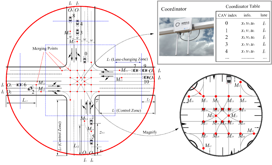
Figure 1: The multi-lane intersection problem. Collisions may happen at the MPs (red dots shown in above figure).

We label the lanes from $l_{1}$ to $l_{8}$ in a counterclockwise direction with corresponding origins $O_{1}$ to $O_{8}$. The rightmost lanes in each direction only allow turning right or going straight, while the leftmost lanes only allow turning left or going straight. However, all CAVs have three possible actions: going straight, turning left, and turning right. Thus, some CAVs must change their lanes so as to execute an action, e.g., left-turning CAV $2$ in $l_{2}$ in Fig. 1. Due to such lane-changing behavior, a new MP $M_{2,1}$ is generated since a conflict of CAV $2$ with a CAV in $l_{1}$ may arise. Similarly, possible MPs may also appear in other lanes when vehicles perform lane-changing maneuvers, as the red dots ($M_{i,2},M_{i,3},\cdots$, and $M_{i,8}$) indicate in Fig. 1. Moreover, it is worth noting that if a CAV needs to change lanes, then it has to travel an additional distance; we assume that this extra distance is a constant $l>0$. In what follows, we consider an intersection which has two lanes in each direction, one of the most common intersection configurations worldwide, and observe that this model is easy to generalize to intersections with more than two lanes.

The intersection has a coordinator (typically a Road Side Unit (RSU)) whose function is to maintain the crossing sequence and all individual CAV information. The most common crossing sequence is based on the FIFO queue of all CAVs, regardless of lanes, using their arrival time at the CZ. The FIFO queue is fair and simple to implement, however, its performance can occasionally be poor. Thus, various cooperative driving strategies have been proposed to generate a more promising crossing sequence, as in [13, 14, 20]. Our approach for controlling CAVs does not depend on the specific crossing sequence selected. Therefore, we first use the FIFO queue so as to enable accurate comparisons with related work also using this scheme and then generalize it to include other resequencing methods which adjust the crossing sequence whenever there is a new arriving vehicle, e,g., the DR method in [13]. This allows CAVs to overtake other CAVs in the CZ from different roads, which better captures actual intersection traffic behaviors.

We begin by reviewing the same basic model as in previous work [11], which will allow us to make accurate comparisons. When a CAV enters the CZ, the coordinator will assign it a unique index. Let $S(t)$ be the set of FIFO-ordered CAV indices and $N(t)$ be the cardinality of $S(t)$. Based on $S(t)$, the coordinator stores and maintains an information table, as shown in Fig. 1. For example, the current lane of CAV $2$ changes from $l_{2}$ to $l_{1}$ after it completes a lane-changing maneuver. In addition, after CAV $0$ passes the intersection, its index will be dropped from the table and the indices of all other CAVs decrease by one. This table enables each CAV to quickly identify CAVs that have potential collisions with it and to optimize its trajectory to maximize some specific objectives. The search algorithm for identifying conflicting vehicles will be introduced in detail in the next section.

The vehicle dynamics for CAV $i$ take the form

$$\left[\begin{array}[c]{c}\dot{x}_{i}(t)\\ \dot{v}_{i}(t)\end{array}\right]=\left[\begin{array}[c]{c}v_{i}(t)+w_{i,1}(t)\\ u_{i}(t)+w_{i,2}(t)\end{array}\right],$$ (1)

where $x_{i}(t)$ is the distance to its origin $O_{j}$ along the lane that CAV $i$ is located in when it enters the CZ, $v_{i}(t)$ denotes the velocity, and $u_{i}(t)$ denotes the control input (acceleration). Moreover, to compensate for possible measurement noise and modeling inaccuracy, we use $w_{i,1}(t),w_{i,2}(t)$ to denote two random processes defined in an appropriate probability space.

II-A Optimization Problem

Based on the notation established above, we can now view trajectory planning of vehicles as an optimization problem where we consider two objectives for each CAV subject to three constraints, including the rear-end safety constraint with the preceding vehicle in the same lane, the lateral safety constraints with vehicles in the other lanes, and the vehicle physical constraints, as detailed next.

Objective 1 (Minimize travel time): Let $t_{i}^{0}$ and $t_{i}^{f}$ denote the time that CAV $i$ arrives at the origin and the time that it leaves the intersection, respectively. To improve traffic efficiency, we wish to minimize the travel time $t_{i}^{f}-t_{i}^{0}$ for CAV $i$.

Objective 2 (Minimize energy consumption): Apart from traffic efficiency, another objective is energy efficiency. Ignoring any noise terms in (1) for the time being, since energy consumption is a monotonic function of the acceleration control input, an energy consumption function we use is defined as

$$J_{i}=\int_{t_{i}^{0}}^{t_{i}^{f}}\mathcal{C}(u_{i}(t))dt,$$ (2)

where $\mathcal{C}(\cdot)$ is a strictly increasing function of its argument.

Constraint 1 (Rear-end safety constraint): Let $i_{p}$ denote the index of the CAV which physically immediately precedes $i$ in the CZ (if one is present). To avoid rear-end collisions, we require that the spacing $z_{i,i_{p}}(t)\equiv x_{i_{p}}(t)-x_{i}(t)$ be constrained by:

$$z_{i,i_{p}}(t)\geq\varphi v_{i}(t)+\delta,\text{ \ }\forall t\in[t_{i}^{0},t_{i}^{m}],$$ (3)

where $\delta$ is the minimum safety distance, and $\varphi$ denotes the reaction time (as a rule, $\varphi=1.8s$ is suggested, e.g., [21]). If we define $z_{i,i_{p}}$ to be the distance from the center of CAV $i$ to the center of CAV $i_{p}$, then $\delta$ is a constant determined by the length of these two CAVs (thus, $\delta$ is generally dependent on CAVs $i$ and $i_{p}$ but taken to be a constant over all CAVs in the sequel, only for simplicity). Note that $i_{p}$ may change when a lane change event or an overtaking event (discussed in Section III.B) occurs.

Constraint 2 (Lateral safety constraint): Let $t_{i}^{k}$ denote the time that CAV $i$ arrives at the MP $M_{k},k\in\{1,2,\dots,32\}$. CAV $i$ may collide with other vehicles that travel through the same MP with it. For all MPs, including the floating MPs $M_{i,l}$ due to lane-changing, there must be enough safe space when CAV $i$ is passing through, that is,

$$z_{i,j}(t_{i}^{k})\geq\varphi v_{i}(t_{i}^{k})+\delta_{i},$$ (4)

where CAV $j\neq i$ is a CAV that may collide with $i$ (note that $j$ may not exist and that there may also be multiple CAVs indexed by $j$ for which this constraint applies at different $t_{i}^{k}$). The determination of $j$ is challenging, and will be addressed in the following section. Compared with related work that requires no more than one CAV within a conflict (or merging) zone at any time, we use (4) to replace this conservative constraint. Instead of such a fixed zone, the space around the MPs to define collision avoidance now depends on the CAV’s speed (and possibly size if we allow $\delta_{i}$ to be CAV-dependent), hence it is much more flexible.

Constraint 3 (Vehicle physical limitations): Due to the physical limitations on motors and actuators, there are physical constraints on the velocity and control inputs for each CAV $i$:

$$v_{min} \leq v_{i}(t)\leq v_{max},\forall t\in[t_{i}^{0},t_{i}^{m}],$$ (5)

$$u_{i,min} \leq u_{i}(t)\leq u_{i,max},\forall t\in[t_{i}^{0},t_{i}^{m}],$$

where $v_{max}>0$ and $v_{min}\geq 0$ denote the maximum and minimum velocity allowed in the CZ, while $u_{i,min}<0$ and $u_{i,max}>0$ denote the minimum and maximum control input for each CAV $i$, respectively.

Similar to prior work, we use a quadratic function for $\mathcal{C}(u_{i}(t))$ in (2) and thus minimize energy consumption by minimizing the control input effort $\frac{1}{2}u_{i}^{2}(t)$. By normalizing travel time and $\frac{1}{2}u_{i}^{2}(t)$, and using $\alpha\in[0,1)$, we construct a convex combination as follows:

$$\begin{aligned} \min_{u_{i}(t),t_{i}^{m}}\int_{t_{i}^{0}}^{t_{i}^{m}}\left(\alpha+\frac{(1-\alpha)\frac{1}{2}u_{i}^{2}(t)}{\frac{1}{2}\max\{u_{max}^{2},u_{min}^{2}\}}\right)dt\end{aligned}.$$ (6)

If $\alpha=1$, the problem (6) is equivalent to a minimum travel time problem; if $\alpha=0$, it becomes a minimum energy consumption problem.

By defining $\beta\equiv\frac{\alpha\max\{u_{\max}^{2},u_{\min}^{2}\}}{2(1-\alpha)}$ (assuming $\alpha<1$) and multiplying (6) by the constant $\frac{\beta}{\alpha}$, we have:

$$\min_{u_{i}(t),t_{i}^{m}}\beta(t_{i}^{m}-t_{i}^{0})+\int_{t_{i}^{0}}^{t_{i}^{m}}\frac{1}{2}u_{i}^{2}(t)dt,$$ (7)

where $\beta\geq 0$ is a weight factor that can be adjusted through $\alpha\in[0,1)$ to penalize travel time relative to the energy cost. Then, the optimization problem can be stated as:

Problem 1

For each CAV $i$ governed by dynamics (1) ignoring noise terms, determine a control law such that (7) is minimized subject to (1), (3), (4), (5), given $t_{i}^{0}$ and the initial and final conditions $x_{i}(t_{i}^{0})=0$, $v_{i}(t_{i}^{0})$, $x_{i}(t_{i}^{m})$.

III Multi-lane Intersection Problem Solution

The solution of Problem 1 can be obtained as described in [15] where a single MP is involved in a two-road single-lane merging configuration where the value of $j$ in (4) is immediately known. The difficulty here is that there may be more than one CAV $j$ defining lateral safety constraints for any $i\in S(t)$ and determining the value(s) of $j$ is challenging since there are eight lanes and three possible actions at intersections as shown in Fig. 1. Obviously, this can become even harder as more lanes are added or asymmetrical intersections are considered. Therefore, we propose a general MP-based approach which involves two steps. The first step addresses the following two issues: $(i)$ A strategy for determining “floating” MPs due to CAVs possibly changing lanes within the CZ, $(ii)$ A strategy for determining all lateral safety constraints, hence the values of $j$ in (4). Once these issues are addressed in the remainder of this section, Problem 1 is well-defined. The second step consists of solving Problem 1 and developing the proposed joint optimal control and barrier function controller in the next section. The overall process is outlined in Algorithm 1 which is implemented in time-driven manner by replanning the control inputs of all CAVs every $T$ seconds.

Algorithm 1 A MP-based Algorithm for Multi-lane intersection problems

1:  Initialize an empty queue table $S(t)$.

2:  for every $T$ seconds do

3:     if a new vehicle enters the CZ then

4:        Determine a passing order for all CAVs according to the FIFO rule or other resequencing methods, e.g., the DR scheme.

5:        Plan an unconstrained optimal control trajectory for the new CAV.

6:        if the new CAV needs to change lanes then

7:           Use the lane-changing MP determination strategy (Section III.A) to determine the lane-changing location and time for the new CAV

8:        end if

9:        Add the information of the new CAV into $S(t)$.

10:     end if

11:     for each CAV in $S(t)$ do

12:        Use the lateral safety constraint determination strategy (Section III.B) to determine which constraints it needs to meet.

13:        Use the joint optimal control and barrier function controller (Section IV) to obtain control inputs for it.

14:        if this CAV has left the intersection then

15:           Remove the information of this CAV from $S(t)$.

16:        end if

17:     end for

18:  end for

III-A Determination of Lane-changing MPs

When a new CAV $i\in S(t)$ arrives at the origins $O_{2},O_{4},O_{6},O_{8}$ (or $O_{1},O_{3},O_{5},O_{7}$) and must turn left (or right), it has to change lanes before getting close to the intersection. Therefore, CAV $i$ must determine the location of the variable (floating) MP $M_{i,k},$ $k\in\{1,2,\cdots,8\}$.

There are three important observations to make:

$(i)$ The unconstrained optimal control for such $i$ is independent of the location of $M_{i,k},$ $k\in\{1,2,\cdots,8\}$ since we have assumed that lane-changing will only induce a fixed extra length $l$ regrdless of where it occurs.

$(ii)$ The optimal control solution under the lateral safety constraint is better (i.e., lower cost in (7)) than one which includes an active rear-end safety constrained arc in its optimal trajectory. This is because the former applies only to a single time instant $t_{i}^{k}$ whereas the latter requires the constraint (3) to be satisfied over all $t\in[t_{i}^{0},t_{i}^{k}]$. It follows that any MP $M_{i,k}$ should be as close as possible to the intersection (i.e., $L_{i,k}$ should be as large as possible, and its maximum value is $L_{2}+L_{3}$), since the lateral safety constraint after $M_{i,k}$ will become a rear-end safety constraint with respect to some $j$ in the adjacent lane.

$(iii)$ In addition, CAV $i$ may also be constrained by its physically preceding CAV $i_{p}$ (if one exists) in the same lane as $i$. In this case, CAV $i$ needs to consider both the rear-end safety constraint with $i_{p}$ and the lateral safety constraint with some $j\neq i$. Thus, the solution is more constrained (hence, more sub-optimal) if $i$ stays in the current lane after the rear-end safety constraint due to $i_{p}$ becomes active. We conclude that in this case CAV $i$ should change its lane to the left (right) lane as late as possible, i.e., just as the rear-end safety constraint with $i_{p}$ first becomes active, i.e., $L_{i,k}$ is determined by

$$L_{i,k}=x_{i}^{\ast}(t_{i}^{a})$$ (8)

where $x_{i}^{\ast}(t)$ denotes the unconstrained optimal trajectory of CAV $i$ (as determined in Sec. IV), and $t_{i}^{a}\geq t_{i}^{0}$ is the time instant when the rear-end safety constraint between $i$ and $i_{p}$ first becomes active; if this constraint never becomes active, then $L_{i,k}=L_{2}+L_{3}$. The value of $t_{i}^{a}$ is determined from (3) by

$$x_{i_{p}}^{\ast}(t_{i}^{a})-x_{i}^{\ast}(t_{i}^{a})=\varphi v_{i}^{\ast}(t_{i}^{a})+\delta,$$ (9)

where $x_{i_{p}}^{\ast}(t)$ is the unconstrained optimal position of CAV $i_{p}$ and $v_{i}^{\ast}(t)$ is the unconstrained optimal speed of CAV $i$. If, however, CAV $i_{p}$’s optimal trajectory itself happened to include a constrained arc, then (9) is only an upper bound of $t_{i}^{a}$.

In summary, it follows from $(i)-(iii)$ above that if CAV $i$ never encounters a point in its current lane where its rear-end safety constraint becomes active, we set $L_{i,k}=L_{2}+L_{3}$, otherwise, $L_{i,k}$ is determined through (8)-(9).

We note that the distances from the origins $O_{1},\dots,O_{8}$ to MPs are not all the same, and the CAVs that make a lane change will induce an extra $l$ distance. Therefore, we need to perform a coordinate transformation for those CAVs that are in different lanes and will meet at the same MP $M_{k},$ $k\in\{1,\dots,32\}$. In other words, when $i\in S(t)$ obtains information for $j\in S(t)$ from the FIFO queue table to account for the lateral safety constraint at an MP $M_{k}$, the position information $x_{j}(t)$ is transformed into $x_{j}^{\prime}(t)$ through

$$x_{j}^{\prime}(t):=\left\{\begin{array}[c]{rcl}x_{j}(t)+L_{i,k}-L_{j,k}+l,&\mbox{if only $i$ changes lane}&\\ x_{j}(t)+L_{i,k}-L_{j,k}-l,&\mbox{if only $j$ changes lane},&\\ x_{j}(t)+L_{i,k}-L_{j,k},&\mbox{otherwise}.&\end{array}\right.$$ (10)

where $L_{i,k},L_{j,k}$ denote the distances of the MPs $M_{k}$ from the origins of CAVs $i$ and $j$, respectively. Note that the coordinate transformation (10) only applies to CAV $i$ obtaining information on $j$ from $S(t)$, and does not involve any action by the coordinator.

III-B Determination of Lateral Safety Constraints

We begin with the observation (by simple inspection of Fig. 1) that CAVs can be classified into two categories, depending on the lane that a CAV arrives at, as follows:

1. The CAVs arriving at lanes $l_{1},l_{3},l_{5},l_{7}$ will pass

   • two MPs if they choose to turn right (including the floating MP $M_{i,k},$ $k\in\{2,4,6,8\}$);

   • four MPs it they turn left;

   • five MPs if they go straight.

2. The CAVs arriving at lanes $l_{2},l_{4},l_{6},l_{8}$ will pass

   • only one MP if they choose to turn right;

   • five MPs if they turn left (including the floating MP $M_{i,k},$ $k\in\{1,3,5,7\}$) or if they go straight.

Clearly, the maximum number of MPs a CAV may pass is 5. Since all such MPs are determined upon arrival at the CZ, we augment the queue table in Fig. 1 by adding the original lane and the MP information for each CAV as shown in Fig. 2 for a snapshot of Fig. 1. The current and original lanes are shown in the third and fourth column, respectively. The original lane is fixed, while the current lane may vary dynamically: in Algorithm 1, the state of all CAVs in the queue is updated if any of them has changed lanes. The remaining five columns show all MPs a CAV will pass through in order. For example, left-turning CAV $2$ in Fig. 1 passes through five MPs $M_{2,1},M_{22},M_{20},M_{17}$, and $M_{13}$ sequentially, where we label the $1$st MP as $M_{2,1}$ and so forth.

Figure 2: The extended coordinator queue table.

When a new CAV enters the CZ, it first determines whether it will change lanes (as described in Section III.A) and identifies all MPs that it must pass. At this point, it looks up the extended queue table $S(t)$ (an example is shown in Fig. 2) which already contains all prior CAV states and MP information. First, from the current lane column, CAV $i$ can determine its current physically immediately preceding CAV $i_{p}$ if one exists. Next, since the passing priority has been determined by the sequencing method selected (FIFO or otherwise), CAVs need to yield to other CAVs that rank higher in the queue $S(t)$. In addition, for any MP CAV $i$ will pass through, it only needs to yield to the closest CAV that has higher priority than it, and this priority is determined by the order of $S(t)$. For instance, CAVs $3$, $4$, and $5$ will all pass through $M_{20}$, as shown in Fig. 2. For the MP $M_{20}$, CAV $5$ only needs to meet the lateral safety constraint with CAV $4$, while the constraint with CAV $3$ will be automatically met since CAV $4$ yields to CAV $3$. Similarly, we can find indices of CAVs for other MPs crossed by CAV $5$. Since CAV $5$ passes through five MPs, we define an index set $\Omega_{5}$ for CAV $5$ which has at most 5 elements. In this example, CAV $5$ only conflicts with CAV $0$ at $M_{29}$ besides $M_{20}$, so that $\Omega_{5}=\{0,4\}$.

Algorithm 2 Search Algorithm for Conflict CAVs

0:  The extended coordinator queue table $S(t)$, CAV $i$

0:  The index of conflict CAVs for CAV $i$

1:  Initialize an empty index set $\Omega_{i}$.

2:  Initialize a set $\Theta_{i}$ including all MPs CAV $i$ will pass through

3:  Find the position $k$ of CAV $i$ in the $S(t)$.

4:  for $j=k-1:-1:1$ do

5:     if the $j$th CAV in $S(t)$ passes at least one MP in $\Theta_{i}$ then

6:        Add the index of this CAV into the set $\Omega_{i}$.

7:        Remove the same MPs from $\Theta_{i}$.

8:     end if

9:     if $\Theta_{i}$ is empty then

10:        break;

11:     end if

12:  end for

13:  return  $\Omega_{i}$

Therefore, it remains to use the information in $S(t)$ in a systematic way so as to determine all the indices of those CAVs that CAV $i$ needs to yield to; these define each index $j$ in (4) constituting all lateral safety constraints that CAV $i$ needs to satisfy. This is accomplished by a search algorithm (Algorithm 2) based on the following process. CAV $i$ compares its original lane and MP information to that of every CAV in the table starting with the last row and moving up. The process terminates the first time that any one of the following three conditions is satisfied at some row $j<i$:

1. All MP information of CAV $i$ matches row $j$ and $\Omega_{i}$ is empty.

2. Every MP for CAV $i$ has been matched to some row $j$.

3. All prior rows $j<i$ have been looked up.

These three conditions are examined in order:

Condition (1): If this is satisfied, there are no conflicting MPs for CAV $i$ and this implies that CAV $i_{p}$ is the physically immediately preceding CAV all the way through the CZ. Thus, CAV $i$ only has to satisfy the safety constraint (3) with respect to $i_{p}$, i.e., it just follows CAV $i_{p}$. For example, $i=4$ and $i_{p}=3$ in Fig. 1 (and Fig. 2).

Condition (2): If this holds, then CAV $i$ has to satisfy several lateral safety constraints with one or more CAV $j\in\Omega_{i}$. Moreover, it also has to satisfy the rear-end safety constraint (3) with CAV $i_{p}$, where $i_{p}$ is determined by the first matched row in the current lane column of Fig. 2. For example, $i=10$, $j=0,1,4,5$, and $6$ in Fig. 1 (and Fig. 2).

Condition (3): There are two cases. First, if the index set $\Omega_{i}$ is empty, then CAV $i$ does not have to satisfy any lateral safety constraint; for example, $i=7$ in Fig. 1. Otherwise, it needs to yield to all CAVs in $\Omega_{i}$; for example, $i=2$, $j=0$ in Fig. 1.

We observe that Algorithm 2 can be implemented for all CAVs in an event-driven way (since $S(t)$ needs to be updated only when an event that changes its state occurs). The triggering events are: $(i)$ a CAV entering the CZ, $(ii)$ a CAV departing the CZ, $(iii)$ a CAV completing a lane change at a floating MP, and $(iv)$ a CAV overtaking event (a lane change event at a fixed MP). This last event may occur when a CAV merges into another lane at a MP through which it leaves the CZ. In particular, consider three CAVs $i,j$, and $k$ such that $k>j>i$, and CAV $j$ merges into the same lane as $i$ and $k$. Then, CAV $k$ looks at the first row above it where there is a CAV with the same lane; that’s now CAV $j$. However, $i$ is physically ahead of $k$. Thus, we need to re-order the queue according to the incremental position order, so that a CAV following $i$ (CAV $k$) can properly identify its physically preceding CAV. For example, consider $i=7$, $j=8$, and $k=9$ in Fig. 1, and suppose that CAV 7 turns right, CAV 8 turns right, and CAV 9 goes straight. Their order in $S(t)$ is 7, 8, 9. CAV 8 can overtake CAV 7, and its current lane will become $l_{6}$ when it passes all MPs. Since CAV 7 and CAV 9 also are in $l_{6}$, CAV 9 will mistake CAV 8 as its new preceding CAV after the current lane of CAV 8 is updated. However, in reality CAV 7 is still the preceding CAV of CAV 9, hence CAV 9 may accidentally collide with CAV 7. To avoid this problem, we need to re-order the queue according to the position information when this event occurs, i.e., making CAV 8 have higher priority than CAV 7 in the queue. Alternatively, this problem may be resolved by simply neglecting CAVs that have passed all MPs when searching for the correct identity of the CAV that precedes $i$.

IV Joint Optimal and Control Barrier Function Controller

Once a newly arriving CAV $i\in S(t)$ has determined all the lateral safety constraints (4) it has to satisfy, it can solve problem (7) subject to these constraints along with the rear-end safety constraint (3) and the state limitations (5). Obtaining a solution to this constrained optimal control problem is computationally intensive, as shown in the single-lane merging problem [15], and this complexity is obviously higher for our multi-lane intersection problem since there are more lateral safety constraints. Therefore, in this section, we proceed in two steps: $(i)$ We solve the unconstrained version of problem (7) which can be done with minimal computational effort, and $(ii)$ We optimally track the unconstrained problem solution while using CBFs to account for all constraints and guarantee they are never violated (as well as Control Lyapunov Functions (CLFs) to better track the unconstrained optimal states). Since this controller $u_{i}(t)$ for CAV $i$ combines an optimal control solution with CBFs, we refer to it as the Optimal Control and Barrier Function (OCBF) control. Note that all CAVs can solve Problem 1 in a decentralized way.

IV-A Unconstrained decentralized optimal control solution

As mentioned above, we use the CAV trajectory obtained from the unconstrained optimal solution Problem 1 as a reference trajectory and deal with all constraints through our OCBF controller. When all state and safety constraints are inactive, we can obtain an analytical solution of Problem 1. As shown in [13], the optimal control, speed, and position trajectories are given by

$$u_{i}^{\ast}(t)=a_{i}t+b_{i}\vspace{-2mm}$$ (11)

$$v_{i}^{\ast}(t)=\frac{1}{2}a_{i}t^{2}+b_{i}t+c_{i}\vspace{-2mm}$$ (12)

$$x_{i}^{\ast}(t)=\frac{1}{6}a_{i}t^{3}+\frac{1}{2}b_{i}t^{2}+c_{i}t+d_{i}$$ (13)

where $a_{i}$, $b_{i}$, $c_{i}$ and $d_{i}$ are integration constants that can be solved along with $t_{i}^{m}$ by the following five algebraic equations (details given in [13]):

$$\frac{1}{2}a_{i}\cdot(t_{i}^{0})^{2}+b_{i}t_{i}^{0}+c_{i}=v_{i}^{0},$$ (14)

$$\frac{1}{6}a_{i}\cdot(t_{i}^{0})^{3}+\frac{1}{2}b_{i}\cdot(t_{i}^{0})^{2}+c_{i}t_{i}^{0}+d_{i}=0,$$

$$\frac{1}{6}a_{i}\cdot(t_{i}^{m})^{3}+\frac{1}{2}b_{i}\cdot(t_{i}^{m})^{2}+c_{i}t_{i}^{m}+d_{i}=L_{k},$$

$$a_{i}t_{i}^{m}+b_{i}=0,$$

$$\beta-\frac{1}{2}b_{i}^{2}+a_{i}c_{i}=0.$$

where the third equation is the terminal condition for the total distance traveled on a lane. This solution is computationally very efficient to obtain. We then use this unconstrained optimal control solution as a reference to be tracked by a controller which uses CBFs to account for all the constraints (3), (4), and (5) and guarantee they are not violated. We review next how to use CBFs to map all these constraints from the state $x_{i}(t)$ to the control input $u_{i}(t)$.

IV-B CBF controller

The OCBF controller aims to track the unconstrained optimal control solution (11)-(13) while satisfying all constraints (3), (5) and (19). To accomplish this, first let $\bm{x}_{i}(t)\equiv(x_{i}(t),v_{i}(t))$. Referring to the vehicle dynamics (1), let $f(\bm{x}_{i}(t))=[x_{i}(t),0]^{T}$ and $g(\bm{x}_{i}(t))=[0,1]^{T}$. Each of the constraints in (3), (5) and (19) can be expressed as $b_{k}(\bm{x}_{i}(t))\geq 0$, $k\in\{1,\cdots,n\}$ where $n$ is the number of constraints and each $b_{k}(\bm{x}_{i}(t))$ is a CBF. For example, $b_{1}(\bm{x}_{i}(t))=z_{i,i_{p}}(t)-\varphi v_{i}(t)-\delta$ for the rear-end safety constraint (3). In the CBF approach, each of the continuously differentiable state constraints $b_{k}(\bm{x}_{i}(t))\geq 0$ is mapped onto another constraint on the control input such that the satisfaction of this new constraint implies the satisfaction of the original constraint $b_{k}(\bm{x}_{i}(t))\geq 0$. The forward invariance property of this method [18, 19] ensures that a control input that satisfies the new constraint is guaranteed to also satisfy the original one. In particular, each of these new constraints takes the form

$$L_{f}b_{k}(\bm{x}_{i}(t))+L_{g}b_{k}(\bm{x}_{i}(t))u_{i}(t)+\gamma(b_{k}(\bm{x}_{i}(t)))\geq 0,$$ (15)

where $L_{f},L_{g}$ denote the Lie derivatives of $b_{k}(\bm{x}_{i}(t))$ along $f$ and $g$ (defined above from the vehicle dynamics) respectively and $\gamma(\cdot)$ denotes a class of $\mathcal{K}$ functions [22] (typically, linear or quadratic functions). As an alternative, a CLF [18] $V(\bm{x}_{i}(t))$, instead of $b_{k}(\bm{x}_{i}(t))$, can also be used to track (stabilize) the optimal speed trajectory (12) through a CLF constraint of the form

$$L_{f}V(\bm{x}_{i}(t))+L_{g}V(\bm{x}_{i}(t))u_{i}(t)+\epsilon V(\bm{x}_{i}(t))\leq e_{i}(t),$$ (16)

where $\epsilon>0$ and $e_{i}(t)$ is a relaxation variable that makes this constraint soft. As is usually the case, we select $V(\bm{x}_{i}(t))=(v_{i}(t)-v_{ref}(t))^{2}$ where $v_{ref}(t)$ is the reference speed to be tracked (specified below). Therefore, the OCBF controller solves the following problem:

$$\small\min_{u_{i}(t),e_{i}(t)}J_{i}(u_{i}(t),e_{i}(t))\!=\!\int_{t_{i}^{0}}^{t_{i}^{m}}\!\left(\beta e_{i}^{2}(t)\!+\!\frac{1}{2}(u_{i}(t)\!-\!u_{ref}(t))^{2}\right)dt,$$ (17)

subject to the vehicle dynamics (1), the CBF constraints (15) and the CLF constraint (16). The obvious selection for speed and acceleration reference signals is $v_{ref}(t)=v_{i}^{\ast}(t)$, $u_{ref}(t)=u_{i}^{\ast}(t)$ with $v_{i}^{\ast}(t)$, $u_{i}^{\ast}(t)$ given by (12) and (11) respectively. In [23], $u_{ref}(t)=\frac{x_{i}^{\ast}(t)}{x_{i}(t)}u_{i}^{\ast}(t)$ is used to provide the benefit of feedback provided by observing the actual CAV trajectory $x_{i}(t)$ and automatically reducing the tracking position error; we use only $u_{ref}(t)=u_{i}^{\ast}(t)$ in the sequel for simplicity.

The CBF conversions from the original constraints to the form (15) are straightforward. For example, using a linear function $\gamma(\cdot)$ in (15), we can directly map Constraint 1 into the following constraint in terms of control inputs:

$$\underbrace{v_{i_{p}}(t)-v_{i}(t)}_{L_{f}b(\bm{x}_{i}(t))}+\underbrace{-\varphi}_{L_{g}b(\bm{x}_{i}(t))}u_{i}(t)+z_{i,i_{p}}(t)-\varphi v_{i}(t)-\delta\geq 0.$$ (18)

However, there are some points that deserve some further clarification as follows.

Constraint 2 (Lateral safety constraint): The lateral safety constraints in (4) are specified only at time instants $t_{i}^{k}$. However, to use CBFs as in (15), they have to be converted to continuously differentiable forms. Thus, we use the same technique as in [24] to convert (4) into:

$$z_{i,j}(t)\geq\Phi(x_{i}(t))v_{i}(t)+\delta,\text{ }i\in S(t),\text{ }t\in[t_{i}^{0},t_{i}^{k}],$$ (19)

where $j\in\Omega_{i}$ is determined through the lateral safety constraint determination strategy (Algorithm 2). Recall that CAV $j$ depends on some MP $M_{k}$ and we may have several $j\in\Omega_{i}$ since CAV $i$ may conflict with several CAVs $j$ at different MPs. The selection of function $\Phi:\mathbb{R}\rightarrow\mathbb{R}$ is flexible as long as it is a strictly increasing function that satisfies $\Phi(x_{i}(t_{i}^{0}))=0$ and $\Phi(x_{i}(t_{i}^{k}))=\varphi$ where $t_{i}^{k}$ is the arrival time at MP $M_{k}$ corresponding to the constraint and $x_{i}(t_{i}^{k})$ is the location of MP $M_{k}$. Thus, we see that at $t=t_{i}^{k}$ all constraints in (19) match the safe-merging constraints (4), and that at $t=t_{i}^{0}$ we have $z_{i,i_{p}}(t_{i}^{0})=\delta$. Since the selection of $\Phi(\cdot)$ is flexible, for simplicity, we define it to have the linear form $\Phi(x_{i}(t))=\frac{\varphi}{x_{i}(t_{i}^{k})}x_{i}(t)$ which we can see satisfies the properties above.

Improving the feasibility of Constraints 1 and 2: In order to ensure that a feasible solution always exists for these constraints, we need to take the braking distance into consideration. CAV $i$ should stop within a minimal safe distance when its speed $v_{i}(t)$ approaches the speed $v_{j}(t)$ for any $j$ such that CAV $j$ is the preceding vehicle of CAV $i$ or any vehicles that may laterally collide with CAV $i$. Thus, we use the following more strict constraint when $v_{i}(t)\geq v_{j}(t)$:

$$z_{i,j}(t)\geq\frac{\varphi\big{(}x_{i}(t)+\frac{1}{2}\frac{v_{i}^{2}(t)-v_{j}^{2}(t)}{u_{\min}}\big{)}v_{j}(t)}{L}+\frac{1}{2}\frac{(v_{j}(t)-v_{i}(t))^{2}}{u_{\min}}+\delta,$$ (20)

A detailed analysis of this constraint is given in [24].

Observing that Constraint 3 (vehicle limitations) can be directly converted using the standard CBF method, we are now in a position where all constraints are mapped into constraints expressed in terms of control inputs. We refer to the resulting control $u_{i}(t)$ in (17) as the OCBF control. The solution to (17) is obtained by discretizing the time interval $[t_{i}^{0},t_{i}^{m}]$ with time steps of length $\Delta$ and solving (17) over $[t_{i}^{0}+k\Delta,t_{i}^{0}+(k+1)\Delta]$, $k=0,1,\ldots$, with $u_{i}(t),$ $e_{i}(t)$ as decision variables held constant over each such interval (see also [24]). Consequently, each such problem is a Quadratic Program (QP) since we have a quadratic cost and a number of linear constraints on the decision variables at the beginning of each time interval. The solution of each such problem gives an optimal control $u_{i}^{\ast}(t_{i}^{0}+k\Delta)$, $k=0,1,\ldots$, allowing us to update (1) in the $k^{th}$ time interval. This process is repeated until CAV $i$ leaves the CZ.

IV-C The influence of noise and complicated vehicle dynamics

Aside from the potentially long computation time, other limitations of the OC controller include: $(i)$ It only plans the optimal trajectory once. However, the trajectory may violate safety constraints due to noise in the vehicle dynamics and control accuracy; $(ii)$ The OC analytical solution is limited to simple vehicle dynamics as in (1) and becomes difficult to obtain when more complicated vehicle dynamics are considered to better match realistic operating conditions. For instance, in practice, we usually need to control the input driving force of an engine instead of directly controlling acceleration. Compared with the OC method, our OCBF approach can effectively deal with the above problems with only slight modifications as described next.

First, due to the presence of noise, constraints may be temporarily violated, which prevents the CBF method from satisfying the forward invariance property. Thus, when a constraint is violated at time $t_{1}$, i.e., $b_{k}(\bm{x}_{i}(t_{1}))<0$, we add a threshold to the original constraint as follows:

$$L_{f}b_{k}(\bm{x}_{i}(t))+L_{g}b_{k}(\bm{x}_{i}(t))u_{i}(t)\geq c_{k}(t),$$ (21)

where $c_{k}(t)\geq 0$ is a large enough value so that $b_{k}(x_{i}(t))$ is strictly increasing even if the system is under the worst possible noise case. Since it is hard to directly determine the value for $c_{k}(t)$, we add it to the objective function and have

$$\small\min_{u_{i}(t),e_{i}(t),c(t)}\quad\int_{t_{i}^{0}}^{t_{i}^{m}}\!\left(\beta e_{i}^{2}(t)\!+\!\frac{1}{2}(u_{i}(t)\!-\!u_{ref}(t))^{2}-\eta c_{k}(t)\right)dt,$$ (22)

where $\eta$ is a weight parameter. If there are multiple constraints that are violated at one time, we rewrite them all as (21) and add all thresholds into the optimization objective. Starting from $t_{1}$, we use the constraint (21) and objective function (22) to replace the original CBF constraint and objective function, and $b_{k}(x_{i}(t))$ will be positive again in finite time since it is increasing. When $b_{k}(x_{i}(t))$ becomes positive again, we revert to the original CBF constraint.

Next, considering vehicle dynamics, there are numerous models which achieve greater accuracy than the simple model (1) depending on the situation of interest. As an example, we consider the following frequently used nonlinear model:

$$\left[\begin{array}[c]{c}\dot{x}_{i}(t)\\ \dot{v}_{i}(t)\end{array}\right]=\left[\begin{array}[c]{c}v_{i}(t)\\ -\frac{1}{m_{i}}F_{r}(v_{i}(t))\end{array}\right]+\left[\begin{array}[c]{c}0\\ \frac{1}{m_{i}}\end{array}\right]u_{i}(t),$$ (23)

where $m_{i}$ denotes the vehicle mass and $F_{r}(v_{i}(t))$ is the resistance force that is normally expressed as

$$F_{r}(v_{i}(t))=\alpha_{0}sgn(v_{i}(t))+\alpha_{1}v_{i}(t)+\alpha_{2}v_{i}^{2}(t),$$ (24)

where $\alpha_{0}>0$, $\alpha_{1}>0$, and $\alpha_{2}>0$ are parameters determined empirically, and $sgn(\cdot)$ is the signum function. It is clear that due to the nonlinearity in these vehicle dynamics, it is unrealistic to expect an analytical solution for it. However, in our proposed OCBF method, we only need to derive the Lie derivative along these new dynamics and solve the corresponding QP based on these new CBF constraints. For instance, it is easy to see that for these new dynamics, the CBF constraint (18) becomes

$$\underbrace{v_{i_{p}}(t)-v_{i}(t)+\frac{\varphi F_{r}(v_{i}(t))}{m_{i}}}_{L_{f}b(\bm{x}_{i}(t))}+\underbrace{-\frac{\varphi}{m_{i}}}_{L_{g}b(\bm{x}_{i}(t))}u_{i}(t)$$ (25)

$$+z_{i,i_{p}}(t)-\varphi v_{i}(t)-\delta\geq 0.$$

Thus, our method can be easily extended to more complicated vehicle dynamics dictated by any application of interest.

V SIMULATION RESULTS

To validate the effectiveness of the proposed OCBF method, we compare it to a state-of-the-art method in [11] where CAVs calculate the fastest arrival time to the conflict zone first when they enter the CZ and then derive an energy-time-optimal trajectory. This uses the same objective function (7) as our method. The main differences are: 1) it considers the merging (conflict) zone as a whole and imposes the conservative requirement that any two vehicles that have potential conflict cannot be in the conflict zone at the same time; 2) when it plans an energy-time-optimal trajectory for a new incoming vehicle, it takes all safety constraints into account and thus is time-consuming; 3) the rear-end safety constraints used in [11] only depends on distance, i.e., $\varphi=0$ and $\delta>0$ in (3). Thus, in order to carry out a fair comparison with it, we adopt the same form of rear-end safety constraints, that is,

$$z_{i,i_{p}}(t)\geq\delta,\text{ \ }\forall t\in[t_{i}^{0},t_{i}^{m}].$$ (26)

A complication caused by this choice is that after using the standard CBF method (simply substituting $\varphi=0$ into (18)), the control input should satisfy

$$\underbrace{v_{i_{p}}(t)-v_{i}(t)}_{L_{f}b(\bm{x}_{i}(t))}+\underbrace{0}_{L_{g}b(\bm{x}_{i}(t))}u_{i}(t)+z_{i,i_{p}}(t)-\delta\geq 0,$$ (27)

which violates the condition $L_{g}b(\bm{x}_{i}(t))\neq 0$. This is because we cannot obtain a relationship involving the control input $u_{i}(t)$ from the first-order derivative of the constraint (26). This problem was overcome in [19] by using a high order CBF (HOCBF) of relative degree 2 for system (1). In particular, letting $b_{k}(\bm{x}_{i}(t))=z_{i,i_{p}}(t)-\delta$ and considering all class $\mathcal{K}$ functions to be linear functions, we define

$$\begin{split}&\psi_{1}(\bm{x}_{i}(t))=\dot{b}(\bm{x}_{i}(t))+pb(\bm{x}_{i}(t),\\ &\psi_{2}(\bm{x}_{i}(t))=\dot{\psi_{1}}(\bm{x}_{i}(t))+p\psi_{1}(\bm{x}_{i}(t)).\end{split}$$ (28)

where $p$ is a (tunable) penalty coefficient. Combining the vehicle dynamics (1) with (28), any control input should satisfy

$$\underbrace{0}_{L_{f}^{2}b(\bm{x}_{i}(t))}+\underbrace{-1}_{L_{g}L_{f}b(\bm{x}_{i}(t))}u_{i}(t)+2p\dot{b}(\bm{x}_{i}(t))+p^{2}b(\bm{x}_{i}(t))\geq 0.$$ (29)

Thus, in the following simulation experiments, we set $\varphi$ for Constraint 1 and Constraint 2 to be $\varphi=0$ and $\varphi=1.8s$, respectively.

Our simulation experiments are organized as follows. First, in Section V.A we consider an intersection with a single lane in each direction which only allows going straight. Our purpose here is to show that using MPs instead of an entire arbitrarily defined conflict zone can effectively reduce the conservatism of the latter. Then, in Section V.B, we allow turns so as to analyze the influence of different behaviors (going straight, turning left, and turning right) on the performance of the methods compared. Next, Section V.C is intended to validate the effectiveness of our OCBF method for intersections with two lanes and include possible lane-changing behaviors. In Section V.D, we extend our method to combine it with the DR method and show that the performance of the OCBF+DR method is better than the OCBF+FIFO method for asymmetrical intersections. Finally, Section V.E demonstrates that our method can effectively deal with complicated vehicle dynamics and noise.

The baseline for our simulation results uses SUMO, a microscopic traffic simulation software package. Then, we use our OCBF controller and the controller proposed in [11] to control CAVs for intersection scenarios with the same vehicle arrival patterns as SUMO. The parameter settings (see Fig. 1) are as follows: $L1=300m$, $L2=50m$, $L_{3}=200m$, $l=0.9378m$, $w=3.5m$, $r=4m$, $\delta=10m$, $v_{\max}=15m/s$, $v_{\min}=0m/s$, $u_{\max}=3m/s^{2}$, and $u_{\min}=-3m/s^{2}$.

The energy model we use in the objective function is an approximate one. The $\frac{1}{2}u^{2}$ metric treats acceleration and deceleration the same and does not account for speed as part of energy. This metric is viewed as a simple surrogate function for energy or simply as a measure of how much the solution deviates from the ideal constant-speed trajectory. In contrast, the following energy model [25] captures fuel consumption in detail and provides another measure of performance:

$$\begin{split}&F_{i}=\int_{0}^{a_{i}}f_{V,i}(t)dt,\\ &f_{V,i}(t)=f_{cruise,i}(t)+f_{accel,i}(t),\\ &f_{cruise,i}(t)=b_{0}+b_{1}v_{i}(t)+b_{2}v_{i}^{2}(t)+b_{3}v_{i}^{3}(t),\\ &f_{accel,i}(t)=u(t)(c_{0}+c_{1}v_{i}(t)+c_{2}v_{i}^{2}(t)),\end{split}$$ (30)

where $f_{cruise,i}(t)$ denotes the fuel consumed per second when CAV $i$ drives at a steady velocity $v_{i}(t)$, and $f_{accel,i}(t)$ is the additional fuel consumed due to the presence of positive acceleration. If $u(t)\leq 0$, then $f_{accel,i}(t)$ will be 0 since the engine is rotated by the kinetic energy of the CAV in this case. $b_{0},b_{1},b_{2},b_{3},c_{0},c_{1}$, and $c_{2}$ are seven model parameters, and here we use the same parameters as in [25], which are obtained through curve-fitting for data from a typical vehicle.

V-A MPs versus conflict zone

In this experiment, we only allow CAVs to go straight in order to investigate the relative performance of the MP-based method (our OCBF controller) and the merging (conflict) zone-based method (OC controller) [11]. We set the arrival rates at all lanes the same, i.e., 270 veh/h/lane. The comparison results are shown in Table I.

TABLE I: The comparison results for a single-lane intersection disallowing turns

$\beta$	Methods	Energy	Travel time (s)	Fuel (mL)	Ave. obj.1
0.1	SUMO	23.1788	28.3810	30.3597	26.0169
	OC	0.1498	28.3884	14.6266	2.9886
	OCBF	0.9501	25.0863	18.3088	3.4587
0.5	SUMO	23.1788	28.3810	30.3597	37.3693
	OC	0.6515	26.0315	17.1585	13.6673
	OCBF	2.1708	22.6623	18.9396	13.5020
1	SUMO	23.1788	28.3810	30.3597	51.5598
	OC	0.8782	25.6961	17.1555	26.5743
	OCBF	2.9106	22.2617	18.9589	25.1723
2	SUMO	23.1788	28.3810	30.3597	79.9408
	OC	1.1869	25.4834	17.1658	52.1537
	OCBF	3.9157	21.9139	18.9852	47.7435

• Ave. obj. = $\beta\times$ Travel time + Energy.

It is clear that both controllers significantly outperform the results obtained from the SUMO controller which employs a standard car following model. The OC controller is the energy-optimal since it has considered all safety constraints at the initial time for each CAV. Then, CAVs strictly follow the planned trajectory assuming that noise is absent. However, for our controller, we only use an unconstrained reference trajectory and employ CBFs to account for the fact that the reference trajectory may violate the safety constraints: the OCBF controller in each CAV continuously updates its control inputs according to the latest states of other CAVs. As a result, its energy consumption is larger than that of the OC controller, although still small and much less than under the SUMO car following controller.

In terms of travel time, we find that the travel time of the OCBF controller is better than that of the OC controller. This is because the safety requirements in the OC controller are too strict so that a CAV $i$ must wait until a CAV $j\neq i$ that conflicts with it leaves the conflict zone. Instead, the OCBF controller using MPs allows us to relax a merging constraint and still ensure safety by requiring that one CAV only can arrive at the same MP $\varphi$ seconds after the other vehicle leaves. Since our method reduces conservatism, it shows significant improvement in travel time when compared with the OC controller in [11].

In addition, we can adjust the parameter $\beta$ to emphasize the relative importance of one objective (energy or time) relative to the other. If we are more concerned about energy consumption, we can use a smaller $\beta$; otherwise, we can use a larger $\beta$ to emphasize travel time reduction. Thus, when $\beta$ is relatively large, the average objective of the OCBF controller is better than that of the OC controller since it is more efficient with respect to travel time.

Another interesting observation is that even though the relationship between the accurate fuel consumption model and the estimated energy is complicated, we see that a larger estimated energy consumption usually corresponds to larger fuel consumption. Thus, it is reasonable to optimize energy consumption through a simple model, e.g., $\frac{1}{2}u^{2}$, which also significantly reduces the computational complexity caused by the accurate energy model.

V-B The influence of turns

In this experiment, we allow turns at the intersection assuming that the behavior of a CAV when it enters the CZ is known. We have conducted four groups of simulations as shown in Table II. In the first group, all CAVs choose their behavior with the same probability, i.e., $\frac{1}{3}$ going straight, $\frac{1}{3}$ turning left, and $\frac{1}{3}$ turning right. In the second group, 80% of CAVs turn left while 10% CAVs go straight and 10% CAVs turn right. In the third group, 80% CAVs turn right while 10% CAVs go straight and 10% CAVs turn left. In the fourth group, 80% CAVs go straight while 10% CAVs turn left and 10% CAVs turn right. We set $\beta=1$ in all results shown in Table II.

TABLE II: The influence of turns on different controllers

Groups	Methods	Energy	Travel time	Fuel	Ave. obj.
1	SUMO	23.7011	28.2503	28.3357	51.9514
	OC	1.2957	22.4667	18.8433	23.7624
	OCBF	2.6193	21.8514	18.9208	24.4707
2	SUMO	26.5612	31.3822	29.0524	57.9434
	OC	1.0666	24.2179	18.0072	25.2845
	OCBF	2.4537	21.8707	18.8704	24.3244
3	SUMO	19.9066	24.2937	25.6778	44.2003
	OC	1.3775	22.0706	18.8803	23.4481
	OCBF	2.3623	21.4874	18.8306	23.8497
4	SUMO	21.7450	26.6148	29.4484	48.3598
	OC	1.2602	22.7417	18.7339	24.0019
	OCBF	2.5884	22.0114	18.9230	24.5998

First, we can draw the same conclusion as in Table I that the OC controller is energy-optimal and the OCBF controller achieves the smallest travel time since it reduces conservatism. Next, we also observe that when we increase the ratio of left-turning vehicles, the average travel times under all controllers increase; when we increase the ratio of right-turning vehicles, the average travel times all decrease. This demonstrates that the left-turning behavior usually has the biggest impact on traffic coordination since left-turning CAVs cross the conflict zone diagonally and are more likely to conflict with other CAVs. In addition, it is worth noting that going straight produces the largest travel time since this involves the largest number of MPs. However, when we use the OCBF controller, the travel times under all situations are similar, which shows that this controller can utilize the space resources of the conflict zone and handle the influence of turns more effectively .

V-C Comparison results for more complicated intersections

In this experiment, we consider more complicated intersections with two lanes in each direction as shown in Fig. 1. The left lane in each direction only allows going straight and turning left, while the right lane only allows going straight and turning right. We set the arrival rate at all lanes to be the same, i.e., 180 veh/h/lane and disallow lane-changing. Each new incoming CAV chooses its behavior from the allowable behaviors with the same probability, e.g., the CAV arriving at the entry of the left lane can go straight or turn left with probability $0.5$. The comparison results are shown in Table III.

TABLE III: Comparison results for a two-lane intersection

$\beta$	Methods	Energy	Travel time (s)	Fuel (mL)	Ave. obj.
0.1	SUMO	24.0124	29.5955	30.5588	26.9720
	OC	0.1514	28.5711	14.6685	3.0085
	OCBF	1.0350	25.0804	18.5086	3.5430
0.5	SUMO	24.0124	29.5955	30.5588	38.8102
	OC	0.6722	26.1284	17.2866	13.7364
	OCBF	2.2244	22.6351	19.0753	13.5420
1	SUMO	24.0124	29.5955	30.5588	53.6079
	OC	0.9063	25.8000	17.2933	26.7063
	OCBF	2.9955	22.2347	19.1126	25.2302
2	SUMO	24.0124	29.5955	30.5588	83.2034
	OC	1.2294	25.5773	17.3042	52.3840
	OCBF	4.2353	22.1167	19.1500	48.4687

The results here are similar to those in the single-lane intersections. Although the number of MPs increases with the number of lanes, our method can still effectively ensure safety and reduce travel time. It is worth noting that the values of safety time headway for the OC controller are difficult to determine. The OC controller requires that no CAV can enter the conflict zone until the conflict CAV leaves it. However, the time spent for passing through the conflict zone differs from vehicle to vehicle. If we choose a larger value, then this significantly increases travel time and amplifies conservatism. In contrast, if we choose a smaller value, the potential of collision increases. Therefore, the MP-based method is significantly better since it not only ensures safety but also reduces conservatism.

Next, we consider the impact of lane-changing on our OCBF method. For the same two-lane intersection, we allow lane-changing and CAVs can choose any actions (going straight, turning left and right). Since the left lane only allows going straight and turning left, the right-turning CAV in this lane must change its lane. The situation is similar for the left-turning CAV in the right lane. To make a better comparison with the scenario without lane-changing, we use the same arrival data (including the times all CAVs enter the CZ and initial velocities) as the last experiment and only change the lane that the turning CAV arrives at. For example, the left-turning CAVs must arrive at the left lane in the last experiment, but in this experiment, the lane they enter into can be random. The results are shown in Table IV.

TABLE IV: The influence of lane-changing behaviour on the proposed method.

$\beta$	Methods	Energy	Travel time	Fuel	Ave. obj.
0.1	SUMO with LC	23.9988	30.0337	30.0000	27.0022
	OCBF w/o LC	1.0350	25.0804	18.5086	3.5430
	OCBF with LC	1.0738	25.1200	18.5474	3.5858
0.5	SUMO with LC	23.9988	30.0337	30.0000	39.0157
	OCBF w/o LC	2.2244	22.6351	19.0753	13.5420
	OCBF with LC	2.2584	22.6689	19.1148	13.5929
1	SUMO with LC	23.9988	30.0337	30.0000	54.0325
	OCBF w/o LC	2.9955	22.2347	19.1126	25.2302
	OCBF with LC	3.0282	22.2684	19.1575	25.2966
2	SUMO with LC	23.9988	30.0337	30.0000	84.0662
	OCBF w/o LC	4.2353	22.1167	19.1500	48.4687
	OCBF with LC	4.2887	22.1536	19.2457	48.5959

We can see that the lane-changing behavior slightly increases all performance measures compared with the results in scenarios disallowing lane-changing. This is expected since a new (floating) MP is added and more control is required to ensure safety. Nevertheless, the changes are small, fully demonstrating the effectiveness of our method in handling lane-changing. Although we have assumed that lane-changing only induces a fixed length, we can extend our OCBF method with more complicated lane-changing trajectories, e.g., trajectories fitted by polynomial functions. Note that in the SUMO simulation, it is assumed that a vehicle can jump directly from one lane to another. However, our method still outperforms it in all metrics, further supporting the advantages of the OCBF method.

Moreover, we explore the effect of asymmetrical arrival rates through two scenarios, in order to confirm that our OCBF method is effective even when traffic flows are heavy. In the first scenario, we set the arrival rates in Lanes 1, 2 to be three times as large as Lanes 3-8; while in the second scenario, the arrival rates in Lanes 1, 2, 5, 6 are three times as large as the remaining lanes. The comparison results are shown in Table V.

TABLE V: The influence of asymmetrical and heavy traffic flows

Sce.	Methods	Energy	Travel time	Fuel	Ave. obj.
1	SUMO	43.1656	68.6488	40.4731	111.8144
	OCBF	2.6312	22.1812	19.1493	24.8124
2	SUMO	44.4815	96.0517	44.6265	140.5332
	OCBF	3.0999	22.5594	19.5380	25.6593

• Scenario 1: the arrival rates at $l_{1}$ and $l_{2}$ are 540 veh/h/lane; while at $l_{3}$ to $l_{8}$ are 180 veh/h/lane.

• Scenario 2: the arrival rates at $l_{1}$, $l_{2}$, $l_{5}$, and $l_{6}$ are 540 veh/h/lane; while at $l_{3}$, $l_{4}$, $l_{7}$, and $l_{8}$ are 180 veh/h/lane.

We can see in the SUMO simulation that traffic flows in lanes with high arrival rates are highly congested with CAVs forming long queues in these lanes. All metrics obtained from SUMO significantly increase compared with the results obtained from medium traffic shown in Table III. However, since the coordination performance of our OCBF is much better than SUMO, all metrics remain at low levels, indicating the effectiveness of our OCBF controller in congested situations.

V-D The inclusion of the DR method

Thus far in our experiments, the FIFO-based queue determines passing priority when potential conflicts happen. This experiment extends our method to combine it with a typical resequencing method, the DR method [13]. When a new CAV enters the CZ, the DR method inserts it into the optimal position of the original crossing sequence. Note that if we combine resequencing methods with the OC method, we need to update the arrival times and trajectories of some CAVs whenever we adjust the original crossing sequence. However, in the OCBF method, CAV $i$ only needs to update its conflicting CAVs according to the new DR-based queue and follow the original unconstrained optimal trajectory without replanning. In the following experiments, we set $\beta=5$ and vary the length of some lanes to generate different scenarios. The comparison results are shown in Table VI.

TABLE VI: The effect of the DR method on the OCBF method

Sce.	Methods	Energy	Travel time	Fuel	Ave. obj.
1	OCBF+FIFO	5.1261	21.6973	19.1518	113.6126
	OCBF+DR	5.1439	21.6404	18.9364	113.3459
2	OCBF+FIFO	5.9218	20.8093	18.6319	109.9683
	OCBF+DR	6.1080	20.6102	18.9077	109.1590
3	OCBF+FIFO	8.9344	19.3548	17.7396	105.7084
	OCBF+DR	7.0501	17.3253	17.2104	93.6766

• Scenario 1 is a symmetrical intersection with all lanes are 300$m$.

• Scenario 2 is an asymmetrical Intersection with lane 3 and 4 are 200$m$ while lane 1, 2, 5, 6, 7, and 8 are 300$m$.

• Scenario 3 is an asymmetrical Intersection with lane 3 and 4 are 200$m$, lane 5 and 6 are 100$m$, while lane 1, 2, 7, and 8 are 300$m$.

The DR method helps decrease travel time and achieves a better average objective value at the expense of energy consumption since CAVs need to do more acceleration/deceleration maneuvers to adjust their crossing sequences. The benefits of the DR method are more significant than the FIFO method for asymmetrical intersections. This is because the FIFO rule may require a CAV that enters the CZ later but is much closer to the intersection to yield to a CAV that is far away from the intersection. For example, in the above Scenario 3, a CAV enters the CZ from lane 5 that is 100 m away from the intersection. It is unreasonable to force it to yield to a CAV entering earlier but at 250 m away from the intersection. Our method with resequencing can effectively avoid producing such situations by replanning crossing sequences in an event-driven way. Note that the OCBF+DR method outperforms the OCBF+FIFO method in all metrics in Scenario 3 since nearly all CAVs arriving at lanes 5 and 6 need to decelerate and even stop due to the FIFO rule, indicating that the DR method is better than the simple FIFO principle when an intersection geometric configuration is asymmetrical.

V-E The influence of nonlinear vehicle dynamics and noise

We first consider the nonlinear vehicle dynamics in (23) and reformulate all CBF constraints according to the new dynamics. For the symmetrical intersection with two lanes in each direction, we vary $\beta$ from 0.1 to 2 and use the OCBF+FIFO method to coordinate the movements of CAVs. The results are shown in Table VII.

TABLE VII: The influence of the nonlinear vehicle dynamics on the OCBF method

$\beta$	Energy	Travel time	Fuel	Ave. obj.
0.1	0.4751	24.5680	16.6496	2.9319
0.5	1.6822	22.3889	18.2822	12.8767
1	2.4702	21.9973	18.4682	24.4675
2	3.4667	21.7871	18.5832	47.0409

It is clear that the results conform to the results for the double integrator vehicle dynamics (1). When $\beta$ increases, we are more concerned about the travel time, thus travel time decreases while the energy and fuel consumption rise. Note that though the nonlinear vehicle dynamics are more complicated than the double integrator vehicle dynamics, the only necessary modification is to derive the CBF constraints based on the new dynamics. The computation times for these two different dynamics are nearly the same.

Next, we have considered both noise and nonlinear dynamics. Due to the measurement errors of sensors and imperfect actuators, there exists random noise in position, velocity, and control inputs. To analyze the influence of noise to the OCBF method, we consider uniformly distributed noise processes ($w_{i,p}(t)$ for the position of CAV $i$, $w_{i,v}(t)$ for the velocity, and $w_{i,u}(t)$ for the control inputs) for this simulation. We set $\beta=0.1$ and use the OCBF+FIFO method for all experiments. The results are shown in Table VIII.

TABLE VIII: The influence of noise on the OCBF method

Noise	Energy	Travel time	Fuel	Ave. obj.
no noise	0.4751	24.5680	16.6496	2.9319
$w_{i,u}(t)\in[-0.5,0.5]$	0.5777	24.6067	16.8714	3.0384
$w_{i,p}(t)\in[-1,1]$	5.4662	24.8587	22.3935	7.9521
$w_{i,v}(t)\in[-1,1]$
$w_{i,p}(t)\in[-1,1]$	5.5723	24.8458	22.3933	8.0569
$w_{i,v}(t)\in[-1,1]$
$w_{i,u}(t)\in[-0.5,0.5]$
$w_{i,p}(t)\in[-2,2]$	31.3250	24.5667	34.1352	33.7817
$w_{i,v}(t)\in[-2,2]$
$w_{i,u}(t)\in[-0.5,0.5]$

The results show that the measurement errors of positions and velocities significantly increase energy consumption. This is because noise causes CAVs to misjudge their states necessitating additional control actions. For example, suppose CAV $i$ is following CAV $j$ and their actual distance is 10 $m$ at some time point, but, due to noise, CAV $i$ may misjudge this distance to be 8 $m$, therefore decelerating to enlarge their relative spacing. Then, at the next time point, it may accelerate to keep a desired inter-vehicle space. These frequent acceleration/deceleration maneuvers cause a considerable waste of energy. As uncertainty increases, more control effort is needed to ensure the safety of CAVs when the number of noise sources increases and the noise magnitudes goes up. Note that CAVs may even collide with other CAVs when we continuously increase the magnitude of noise. However, when noise is limited, our method can effectively handle it and does not add any computational burden.

VI CONCLUSIONS

This paper presents a decentralized optimal control method for controlling CAVs passing through a multi-lane intersection safely while jointly minimizing the travel time and energy consumption of each CAV. First, CAVs calculate the desired trajectory generated by unconstrained optimal control. Then, we design a search algorithm for a CAV to search all lateral safety constraints that it needs to meet with other conflicting CAVs. An OCBF controller is designed to follow the desired trajectory while ensuring all safety constraints and physical vehicle limitations. Multiple simulation experiments we have conducted show that the proposed method can handle complex objective functions, nonlinear vehicle dynamics, the presence of noise, and it is still effective under the influence of lane-changing behavior, heavy traffic flows, and asymmetrical intersections. Our ongoing work includes extensions to large traffic networks and enhancing the feasibility of the QPs in challenging environments where this may not always be the case. Finally, when the CAV trajectories involve curves, we plan to include more complicate lateral dynamics that better model vehicle behavior in such cases.

References

- [1] J. Rios-Torres and A. A. Malikopoulos, “A survey on the coordination of connected and automated vehicles at intersections and merging at highway on-ramps,” IEEE Transactions on Intelligent Transportation Systems, vol. 18, no. 5, pp. 1066–1077, 2016.
- [2] L. Chen and C. Englund, “Cooperative intersection management: A survey,” IEEE Transactions on Intelligent Transportation Systems, vol. 17, no. 2, pp. 570–586, 2015.
- [3] L. Li, D. Wen, and D. Yao, “A survey of traffic control with vehicular communications,” IEEE Transactions on Intelligent Transportation Systems, vol. 15, no. 1, pp. 425–432, 2014.
- [4] R. Hult, G. R. Campos, E. Steinmetz, L. Hammarstrand, P. Falcone, and H. Wymeersch, “Coordination of cooperative autonomous vehicles: Toward safer and more efficient road transportation,” IEEE Signal Processing Magazine, vol. 33, no. 6, pp. 74–84, 2016.
- [5] S. A. Fayazi and A. Vahidi, “Mixed-integer linear programming for optimal scheduling of autonomous vehicle intersection crossing,” IEEE Transactions on Intelligent Vehicles, vol. 3, no. 3, pp. 287–299, 2018.
- [6] H. Xu, S. Feng, Y. Zhang, and L. Li, “A grouping-based cooperative driving strategy for cavs merging problems,” IEEE Transactions on Vehicular Technology, vol. 68, no. 6, pp. 6125–6136, 2019.
- [7] X. Qian, J. Gregoire, A. De La Fortelle, and F. Moutarde, “Decentralized model predictive control for smooth coordination of automated vehicles at intersection,” in 2015 European Control Conference (ECC). IEEE, 2015, pp. 3452–3458.
- [8] H. Xu, Y. Zhang, C. G. Cassandras, L. Li, and S. Feng, “A bi-level cooperative driving strategy allowing lane changes,” Transportation Research Part C: Emerging Technologies, vol. 120, p. 102773, 2020.
- [9] K. Dresner and P. Stone, “A multiagent approach to autonomous intersection management,” Journal of artificial intelligence research, vol. 31, pp. 591–656, 2008.
- [10] A. A. Malikopoulos, C. G. Cassandras, and Y. J. Zhang, “A decentralized energy-optimal control framework for connected automated vehicles at signal-free intersections,” Automatica, vol. 93, pp. 244–256, 2018.
- [11] Y. Zhang and C. G. Cassandras, “Decentralized optimal control of connected automated vehicles at signal-free intersections including comfort-constrained turns and safety guarantees,” Automatica, vol. 109, pp. 1–9, 2019.
- [12] Y. Meng, L. Li, F. Wang, K. Li, and Z. Li, “Analysis of cooperative driving strategies for nonsignalized intersections,” IEEE Transactions on Vehicular Technology, vol. 67, no. 4, pp. 2900–2911, 2018.
- [13] Y. Zhang and C. G. Cassandras, “A decentralized optimal control framework for connected automated vehicles at urban intersections with dynamic resequencing,” in 2018 IEEE Conference on Decision and Control (CDC). IEEE, 2018, pp. 217–222.
- [14] H. Xu, Y. Zhang, L. Li, and W. Li, “Cooperative driving at unsignalized intersections using tree search,” IEEE Transactions on Intelligent Transportation Systems, pp. 1–9, 2019. [Online]. Available: https://ieeexplore.ieee.org/abstract/document/8848467
- [15] W. Xiao and C. G. Cassandras, “Decentralized optimal merging control for connected and automated vehicles,” in 2019 American Control Conference (ACC). IEEE, 2019, pp. 3315–3320.
- [16] W. Xiao, C. G. Cassandras, and C. Belta, “Bridging the gap between optimal trajectory planning and safety-critical control with applications to autonomous vehicles,” Automatica (provisionally accepted, available in arXiv: 2008.07632), 2020.
- [17] A. D. Ames, J. W. Grizzle, and P. Tabuada, “Control barrier function based quadratic programs with application to adaptive cruise control,” in 53rd IEEE Conference on Decision and Control (CDC). IEEE, 2014, pp. 6271–6278.
- [18] A. D. Ames, S. Coogan, M. Egerstedt, G. Notomista, K. Sreenath, and P. Tabuada, “Control barrier functions: Theory and applications,” in 2019 18th European Control Conference (ECC). IEEE, 2019, pp. 3420–3431.
- [19] W. Xiao and C. Belta, “Control barrier functions for systems with high relative degree,” in Proc. of 58th IEEE Conference on Decision and Control, Nice, France, 2019, pp. 474–479.
- [20] W. Xiao and C. G. Cassandras, “Decentralized optimal merging control for connected and automated vehicles with optimal dynamic resequencing,” in Proc. of the American Control Conference, 2020, pp. 4090–4095.
- [21] K. Vogel, “A comparison of headway and time to collision as safety indicators,” Accident analysis & prevention, vol. 35, no. 3, pp. 427–433, 2003.
- [22] H. K. Khalil and J. W. Grizzle, Nonlinear systems. Prentice hall Upper Saddle River, NJ, 2002, vol. 3.
- [23] W. Xiao, C. G. Cassandras, and C. Belta, “Decentralized merging control in traffic networks with noisy vehicle dynamics: a joint optimal control and barrier function approach,” in 2019 IEEE Intelligent Transportation Systems Conference (ITSC). IEEE, 2019, pp. 3162–3167.
- [24] W. Xiao, C. Belta, and C. G. Cassandras, “Decentralized merging control in traffic networks: A control barrier function approach,” in Proc. ACM/IEEE International Conference on Cyber-Physical Systems, Montreal, Canada, 2019, pp. 270–279.
- [25] M. A. S. Kamal, M. Mukai, J. Murata, and T. Kawabe, “Model predictive control of vehicles on urban roads for improved fuel economy,” IEEE Transactions on control systems technology, vol. 21, no. 3, pp. 831–841, 2012.