Cosmic ray positrons from compact binary millisecond pulsars

Abstract

A new population of neutron stars has emerged during the last decade: compact binary millisecond pulsars (CBMSPs). Because these pulsars and their companion stars are in tight orbits with typical separations of $10^{11}$ cm, their winds interact strongly forming an intrabinary shock. Electron-positron pairs reaccelerated at the shock can reach energies of about 10 TeV, which makes this new population a potential source of GeV-TeV cosmic ray positrons. We present an analytical model for the fluxes and spectra of positrons from intrabinary shocks of CBMSPs. We find that the minimum energy $E_{\min}$ of the pairs that enter the shock is critical to quantify the energy spectrum with which positrons are injected into the interstellar medium. We measure for the first time the Galactic scale height of CBMSPs, $z_{\mathrm{e}}=0.4\pm 0.1$ kpc, after correcting for an observational bias against finding them close to the Galactic plane. From this, we estimate a local density of 5–9 kpc^-3 and an extrapolated total of 2–7 thousand CBMSPs in the Galaxy. We then propagate the pairs in the isotropic diffusion approximation and find that the positron flux from the total population is about two times higher than that from the 52 currently known systems. For $E_{\min}$ between 1 and 50 GeV, our model predicts only a minor contribution from CBMSPs to the diffuse positron flux at 100 GeV observed at Earth. We also quantify the effects of anisotropic transport due to the ordered Galactic magnetic field, which can change the diffuse flux from nearby sources drastically. Finally, we find that a single “hidden” CBMSP close to the Galactic plane can yield a positron flux comparable to the AMS-02 measurements at 600 GeV if its line-of-sight to Earth is along the ordered Galactic field lines, while its combined electron and positron flux at higher energies would be close to the measurements of CALET, DAMPE and Fermi-LAT.

1 Introduction

1.1 Cosmic ray positrons and pulsar winds

Measurements of the antimatter fraction of cosmic rays (CRs) are not only valuable probes for cosmology and particle physics, but provide also important insights into astrophysical sources of CRs and their subsequent propagation in the Galaxy [1]. A guaranteed production channel of antimatter are the interactions of CR protons and nuclei with gas in the interstellar medium. If this channel were the main source of antimatter, the energy dependence of the Galactic diffusion coefficient ($D\propto E^{\delta}$ with $\delta=0.3-0.5$) would lead to a decrease of the antimatter fraction with energy, as discussed e.g. in Ref. [2] The rise in the positron-to-electron fraction above 20 GeV, first observed clearly by the PAMELA [3, 4] and then confirmed by the AMS-02 collaboration [5, 6], requires therefore additional sources of positrons. Moreover, the high-energy part of the $e^{\pm}$ spectrum should be dominated by local sources, as pointed out already 30 years ago [7, 8], since high-energy electrons lose energy fast.

Pulsars are natural candidates for such positron sources, because electromagnetic pair cascades in their magnetospheres lead to a large positron fraction, $f_{e^{+}/e^{-}}\simeq 1$, without affecting the antiproton flux. A neutron star with spin period $P$, radius $R$, and surface magnetic field strength $B_{\mathrm{s}}$ must maintain a charge density known as the Goldreich-Julian density [9] to screen the electric field induced by its rotating magnetic field. In order to keep this charge density at a steady state, charged particles are extracted from the neutron star surface and ejected at a rate that can be characterized by the Goldreich-Julian rate [10],

$$\dot{N}_{\mathrm{GJ}}=\frac{4\pi^{2}B_{\mathrm{s}}R^{3}}{2ceP^{2}},$$ (1.1)

of order 10${}^{32}/$s for the pulsars studied here. According to most models [10, 11], these “primary” charges lead to copious pair production inside the pulsar magnetosphere, within the light cylinder defined as the surface where corotating magnetic field lines reach the speed of light $c$, at a radius $R_{\mathrm{lc}}=cP/(2\pi)$. Depending on the pair cascade multiplicity, the rate of “secondary” pairs emerging from the light cylinder can be 1–4 orders of magnitude higher than $\dot{N}_{\mathrm{GJ}}$.

These secondary $e^{\pm}$ pairs escape through the open field lines and feed the relativistic pulsar wind. The contribution of protons and nuclei to the wind and shock in an additional hadronic component has been debated for decades [12]. Pulsar winds are thought to be Poynting flux dominated near the light cylinder, in their innermost parts. In other words, the electromagnetic energy density is thought to dominate over the kinetic energy density of particles just outside the light cylinder, in the inner wind. How and where particles are accelerated as one moves outwards in the wind is an open question (the so-called “sigma problem”; see, e.g., Ref. [10] for a recent review). Reference [13] constrained the transition radius from a magnetically to a kinetically dominated wind, placing it at more than $(5-30)\,R_{\mathrm{lc}}$. But at the distances of interest for our work, with intrabinary shocks at $\sim(10^{3}-10^{4})\,R_{\mathrm{lc}}$, the ratio of magnetic to particle energy density is so far largely unconstrained.

The expected electron and positron fluxes from some pulsars, as well as the resulting anisotropy, have been studied in detail using the isotropic diffusion approximation [14, 15]. Two promising candidates are the relatively young, isolated, gamma-ray pulsars Geminga and PSR B0656+14, which are only (250–300) pc from Earth. Recent HAWC observations of extended TeV gamma-ray emission confirmed that they are local sources of accelerated electrons [16]. However, the presence of electrons with energies in the 10–1000 GeV range in these sources can be tested directly looking for GeV photons using Fermi’s Large Area Telescope (LAT). No GeV photon halo around Geminga and PSR B0656+14 has been found in the search performed in Ref. [17], and the derived upper limits were used to constrain their contribution to the observed positron flux as $\raise 1.29167pt\hbox{$\;<$\kern-7.5pt\raise-4.73611pt\hbox{$\sim\;$}}15\%$. A similar analysis [18] detected a weak GeV halo around Geminga and set an upper limit of $20\%$ to its contribution to the observed positron flux. These limits disfavour these two candidates, and young pulsars in general, as explanation for the positron excess.

An alternative pulsar scenario are pulsar wind nebulae (PWN) with bow shocks [19, 20]. These shocks form when PWNe move relative to the ambient interstellar medium with supersonic speeds. Particles accelerated at the termination surface of the pulsar wind may undergo acceleration in the converging flow formed by the outflow from the wind termination shock and the inflow from the bow shock, leading to very hard energy spectra. Assuming a steepening of the spectrum at $E\simeq 500$ GeV, the measured positron fraction can be reproduced. Because pairs can only be released into the interstellar medium after the pulsar has escaped the supernova remnant ($\sim 10^{4}$ yr after being formed), the predictions of this scenario depend critically on the time evolution of the spin-down rate of the neutron star [19]. Specifically, for the most likely spin-down history the PWN bow shock models require very high efficiencies ($\simeq 30-50\%$) in converting spin-down luminosity into pairs [19, 20].

1.2 Millisecond pulsars in compact binaries

A new class of millisecond pulsars (MSPs) has emerged during the last decade [21, 22, 23], thanks to the Fermi-LAT. These are nearby MSPs (mostly within 3 kpc) in compact binaries (orbital periods $P_{\mathrm{b}}\lesssim 1$ d), with non-degenerate or semi-degenerate companion stars. The former, known as redbacks (RBs), have companions with masses of at least $M_{\mathrm{c,min}}\sim 0.1\,M_{\odot}$ [24], while the latter, known as black widows (BWs) have $M_{\mathrm{c,min}}\sim 0.01\,M_{\odot}$ [25]. We refer to both types as compact binary MSPs (CBMSPs) or “spiders”, after their nicknames inpired by cannibalistic spiders. While in 2008 only four such systems were known, at the moment of writing we know 52 CBMSPs in the Galactic field, so they represent about 20% of the total MSP population (see Section 2.1 for details).

Millisecond pulsars live long (their characteristic age is $P/(2\dot{P})\sim 0.1-10$ Gyr) and have moderately strong winds powered by the loss of rotational energy with spin-down luminosities $L_{\mathrm{sd}}=10^{33}-10^{35}$ erg/s. Since the magnetospheres of MSPs are smaller than those of normal (young, slow) pulsars and that is where the magnetic field decays most rapidly, MSPs have stronger fields than normal pulsars at the light cylinder ($10^{3}-10^{6}$ G) and in the wind. The orbital evolution of CBMSPs also happens on long timescales ($\gtrsim 0.5$ Gyr), driven by the evaporation of the companion or magnetic braking [26, 27]. Since these are much longer than the CR diffusion timescales, CBMSPs can be considered steady sources of CRs, as opposed to quasi-instantaneous sources of CRs like young pulsars or supernova remnants.

Due to their small orbital separations, $a\sim 10^{10}-10^{11}$ cm, the pulsar and its companion can interact strongly, providing a new probe of the innermost pulsar wind. The X-ray emission of CBMSPs indicates the presence of an intrabinary shock between the pulsar and companion winds [28, 29, 30], which can be very efficient at reaccelerating particles [31, 32]. While pair cascades from the magnetospheres of MSPs cut off around a few tens of GeV and thus cannot contribute to the high-energy rise of $f_{e^{+}/e^{-}}$, electron-positrons are accelerated up to tens of TeV in the strong intrabinary shocks of CBMSPs. In particular, the authors of Ref. [33] argued that the contribution of 24 CBMSPs known in 2015 to the positron flux on Earth can reach levels of a few tens of percent at tens of TeV, depending on model parameters.

In this work we examine if the full population of CBMSPs can contribute significantly to the observed positron flux on Earth. To do so, we study the currently known population and estimate the total intrinsic Galactic population in Section 2. In Section 3, we develop a simple analytical model of the electron-positron fluxes and spectra from intrabinary shocks of CBMSPs. We calculate the diffuse positron flux on Earth including effects of anisotropic diffusion (Section 4) and present the resulting diffuse fluxes in Section 5. We briefly discuss and summarize our main results in Section 6.

ID [V15]	Name	type	Pb	a/$\mathrm{10^{10}}$	Mc,min	Ps	Bs/$\mathrm{10^{8}}$	$L_{sd}$/$\mathrm{10^{34}}$	d	x y z	Ref.
-	-	-	$\mathrm{h}$	cm	$\mathrm{M_{\odot}}$	$\mathrm{ms}$	G	$\mathrm{erg\,s^{-1}}$	$\mathrm{kpc}$	$\mathrm{kpc}$	-
1 [18]	J1023+0038	RB	4.8	13	0.2	1.7	2.2	5.7	1.4[0.6]	0.43 0.85 0.98	[34]
2 [0]	J1048+2339	RB	6	15	0.3	4.7	7.6	1.2	0.7	0.27 0.18 0.62	[35]
3 [0]	J1227-4853	RB	6.9	16	0.14	1.7	2.8	9.1	2.5	-1.2 2.1 0.6	[36]
4 [0]	J1306-40	RB	26	-	-	2.2	-	-	1.2	-0.65 0.9 0.45	[37]
5 [0]	J1431-4715	RB	11	22	0.12	2	3.4	6.8	1.5	-1.1 0.94 0.32	[38]
6 [0]	J1622-0315	RB	3.9	11	0.1	3.9	4.3	0.77	1.1	-0.93 -0.18 0.56	[39]
7 [19]	J1628-3205	RB	5	13	0.16	3.2	-	1.4	1.2	-1.1 0.26 0.24	[23]
8 [20]	J1723-2837	RB	15	27	0.24	1.9	2.4	4.7	0.75	-0.75 0.031 0.056	[40]
9 [21]	J1816+4510	RB	8.7	19	0.16	3.2	7.5	5.2	4.5[2.4]	-1.2 -3.9 1.9	[41]
10 [0]	J1908+2105	RB	3.5	10	0.055	2.6	-	-	2.6	-1.5 -2.1 0.26	[42]
11 [0]	J1957+2516	RB	5.7	14	0.1	4	6.7	1.7	3.1	-1.4 -2.8 -0.11	[43]
12 [22]	J2129-0429	RB	15	28	0.37	7.6	-	3.9	0.9	-0.47 -0.54 -0.54	[21]
13 [23]	J2215+5135	RB	4.1	11	0.22	2.6	6	7.4	3	0.51 -2.9 -0.22	[21]
14 [24]	J2339-0533	RB	4.6	12	0.26	2.9	4.1	2.3	1.1[0.4]	-0.076 -0.5 -0.98	[44]
15 [0]	J0212+5320	RBc	21	34	0.3	-	-	-	1.1	0.77 -0.77 -0.15	[45]
16 [0]	J0523-2529	RBc	16	32	0.8	-	-	-	1.1	0.64 0.71 -0.55	[46]
17 [0]	J0744-2523	RBc	2.8	-	-	-	-	-	1.5	0.72 1.3 -0.018	[47]
18 [0]	J0838.8-2829	RBc	5.1	-	-	-	-	-	1	0.33 0.93 0.14	[48]
19 [0]	J0954.8-3948	RBc	9.3	-	-	-	-	-	1.7	0.002 1.7 0.34	[49]
20 [0]	J1302-3258	RBc	15	27	0.15	3.8	-	0.5	0.96	-0.48 0.68 0.48	[22]
21 [0]	J2039-5618	RB	5.4	-	-	2.6	-	-	0.9	-0.68 0.23 -0.54	[50]
22 [0]	J2333.1-5527	RBc	6.9	-	-	-	-	-	3.1	-1.3 0.95 -2.6	[51]
23 [11]	B1957+20	BW	9.2	19	0.021	1.6	3.3	16	2.5[1.5]	-1.3 -2.1 -0.2	[25]
24 [2]	J0610-2100	BW	6.9	16	0.025	3.9	4.4	0.85	3.5	2.2 2.5 -1.1	[52]
25 [13]	J2051-0827	BW	2.4	7.8	0.027	4.5	4.9	0.55	1	-0.7 -0.57 -0.53	[53]
26 [1]	J0023+0923	BW	3.3	9.6	0.016	3	3.8	1.6	0.7	0.15 -0.39 -0.56	[22]
27 [0]	J0251+2606	BW	4.9	13	0.024	2.5	-	-	1.2	0.94 -0.46 -0.59	[42]
28 [0]	J0636+5128	BW	1.6	5.9	0.007	2.9	2	0.56	0.5	0.46 -0.13 0.16	[54]
29 [0]	J0952-0607	BW	6.4	15	0.02	1.4	-	-	0.97	0.35 0.71 0.56	[55]
30 [3]	J1124-3653	BW	5.4	13	0.027	2.4	-	1.6	1.7	-0.38 1.5 0.66	[22]
31 [4]	J1301+0833	BW	6.5	15	0.024	1.8	-	6.7	0.7	-0.15 0.17 0.66	[23]
32 [5]	J1311-3430	BW	1.6	5.8	0.008	2.6	4.7	4.9	1.4	-0.75 0.98 0.66	[56]
33 [6]	J1446-4701	BW	6.7	15	0.0019	2.2	3	3.7	1.5	-1.2 0.9 0.3	[57]
34 [0]	J1513-2550	BW	4.3	11	0.02	2.1	4.3	8.8	2	-0.82 -0.66 1.7	[39]
35 [7]	J1544+4937	BW	2.8	8.6	0.018	2.2	1.6	1.2	1.2	-0.14 -0.75 0.92	[58]
36 [0]	J1641+8049	BW	2.2	7.4	0.04	2	-	4.3	1.7	0.58 -1.3 0.89	[59]
37 [8]	J1731-1847	BW	7.5	17	0.04	2.3	4.9	7.8	2.5	-2.5 -0.3 0.35	[60]
38 [9]	J1745+1017	BW	18	29	0.014	2.6	1.7	0.58	1.3[1.4]	-1.0 -0.7 0.43	[61]
39 [0]	J1805+06	BW	8.1	17	0.023	2.1	-	-	2.5	-2 -1.3 0.56	[42]
40 [10]	J1810+1744	BW	3.6	10	0.044	1.7	-	3.9	2	-1.4 -1.3 0.58	[22]
41 [0]	J1928]+1245	BW	3.3	9.6	0.009	3	1.7	0.24	6.1	-4 -4.6 -0.24	[62]
42 [0]	J1946-5403	BW	3.1	9.2	0.021	2.7	-	-	0.9	-0.75 0.22 -0.44	[63]
43 [0]	J2017-1614	BW	2.3	7.6	0.03	2.3	1.5	0.7	1.1	-0.88 -0.45 -0.49	[39]
44 [12]	J2047+1053	BW	3	9	0.035	4.3	-	1	2	-1.0 -1.6 -0.67	[23]
45 [0]	J2052+1218	BW	2.6	8.2	0.033	2	-	-	3.9	-1.9 -3.1 -1.3	[42]
46 [0]	J2055+3829	BW	3.1	9.2	0.023	2.1	0.93	0.36	4.6	-0.75 -4.5 -0.34	[64]
47 [0]	J2115+5448	BW	3.2	9.4	0.02	2.6	9	16	3.4	0.3 -3.4 0.24	[39]
48 [14]	J2214+3000	BW	10	20	0.014	3.1	4.3	1.9	3.6[1.3]	-0.18 -3.3 -1.3	[65]
49 [15]	J2234+0944	BW	10	20	0.015	3.6	5.5	1.7	1	-0.18 -0.74 -0.65	[57]
50 [16]	J2241-5236	BW	3.4	9.8	0.012	2.2	2.4	2.5	0.5	-0.27 0.11 -0.41	[66]
51 [17]	J2256-1024	BW	5.1	13	0.034	2.3	-	5.2	0.6	-0.16 -0.27 -0.51	[67]
52 [0]	J1653-0159	BWc	1.2	-	-	-	-	-	1	-0.87 -0.26 0.42	[68]

Table 1: Names and properties of the 52 currently known CBMSPs: orbital period P_b and separation a, minimum mass of the companion star M_c,min, pulsar spin period P_s, magnetic field B_s and spin-down luminosity L_sd, as well as distance and Cartesian coordinates. The first column, between square brackets, shows the ID number of the systems studied by Venter et al. [33] (those with [0] were not included/known at the time). ”RB” and ”BW” are redback and black widow sub-types, respectively, and a ”c” denotes those candidate systems with no published detection of pulsations. When these differ from ours, we show between square brackets the distances used by Venter et al. [33]. Median values are: P=2.6 ms, L_sd=2.3$\times$10³⁴ erg s^-1, $\dot{P}$=1.3$\times$10^-20, B_s=3.6$\times$10⁸ G, P_b=5.1 hr, M_c,min=0.16 M_⊙ (RBs), 0.021 M_⊙ (BWs), a=1.3$\times$10¹¹ cm. Note: L_sd values listed as reported (not always corrected for Shklovskii effect, often assume I=10⁴⁵ g cm²). M_c,min values for an edge-on orbit listed as reported (often assume M=1.4 M_⊙ for the pulsar).

2 A growing population of spiders

2.1 Currently known population

Table 1 shows the currently known population of CBMSPs and some of their properties, which we have collected from the literature. We do not include here globular cluster spiders, since most of them are too distant to be relevant for our purposes (there are about 30 known CBMSPs in globular clusters, but all of them are more than 2 kpc away, and only four are between 2 and 4 kpc [69]). Our updated sample includes 52 systems: 22 redbacks (seven of them candidates, where no pulsations have been detected yet, labelled RBc) and 30 black widows (one of them candidate, labelled BWc). The median values of $P$, $L_{\mathrm{sd}}$, $P_{\mathrm{b}}$ and $M_{\mathrm{c,min}}$ are given in Table 1. In the few cases where these measurements are not available (e.g. because no coherent pulsar timing solution has been published) we use such median values as input for the pair spectral model that we will develop in Section 3.

For those systems with reported spin period derivative $\dot{P}$, we calculate the surface magnetic field strength at the equator as

$$B_{\mathrm{s}}=2\sqrt{P\dot{P}\frac{3Ic^{3}}{8\pi^{2}R^{6}}}\,,$$ (2.1)

where we assume $I=2MR^{2}/5$ for the neutron star’s moment of inertia and we use as mass $M=1.85~{}M_{\odot}$ [70] and radius $R=11$ km [71]. We calculate the orbital separation,

$$a=\left(\frac{GM_{\mathrm{tot}}\,P_{b}^{2}}{4\pi^{2}}\right)^{(1/3)},$$ (2.2)

assuming for the total mass in the binary $M_{\mathrm{tot}}=M+M_{\mathrm{c,min}}$. We use refined distance measurements for each system when available (from, e.g., radio parallax [72] or optical observations [73]), and radio-timing dispersion measure estimates otherwise.

We show in Figure 1 (left) the Galactic Cartesian coordinates of the 52 currently known CBMSPs; the coordinate system is centered on the Sun with its $x$ axis pointing towards the Galactic anticenter. The vast majority of CBMSPs have been discovered in systematic radio-timing [22, 21, 23, 60, 57, 61, 63] or optical-photometric [56, 74, 45] searches of unidentified Fermi-LAT gamma-ray sources. To avoid diffuse GeV emission near the Galactic plane, most searches have excluded Galactic latitudes $|\ell|<5^{\circ}$. Thus, there is a strong selection effect against finding CBMSPs near the plane, which is clearly visible in the $z$ distribution shown in Figure 1 (right). Even though the intrinsic number density is expected to increase when approaching the Galactic plane, the observed density of CBMSPs drops off sharply below $|z|\simeq 0.5$ kpc. From this we can predict that at least $\sim$20-50 CBMSPs are “hidden” in the Galactic plane, with $|z|\lesssim 0.5$ kpc. Those systems should be at distances similar to the currently known population (less than 6 kpc) and thus we expect them to be detectable as radio pulsars (at higher dispersion measures), even though their GeV emission may be blended with the Galactic background.

Since the current “horizon” for detection is at approximately 5 kpc (all but one CBMSPs in Table 1 are within 5 kpc from Earth), we estimate that the distribution of $z$ is mostly unbiased for $|z|>5\,{\rm kpc}\sin(5^{\circ})\simeq 0.45$ kpc. By fitting this distribution with an exponential model, we find a scale height $z_{\mathrm{e}}=(0.4\pm 0.1)$ kpc, where the uncertainty is estimated by using different bin sizes (0.1–0.3 kpc) and thresholds for the lowest fitted $z$ values (0.4–0.5 kpc). A Gaussian fit gives a slightly higher yet consistent scale height (0.5 kpc, see Figure 1). This is, to our knowledge, the first determination of the scale height of CBMSPs. Previous population synthesis studies including all types of MSPs found similar values for $z_{\mathrm{e}}$, $0.5^{+0.19}_{-0.13}$ kpc [75, 76]. The population of Galactic low-mass X-ray binaries, from which MPSs are supposed to evolve, also shows a relatively high scale height $z_{\mathrm{e}}=(0.4\pm 0.1)$ kpc [77], in full agreement with our results for CBMSPs.

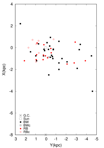
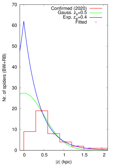
Figure 1: Left: Top view of the $x$ and $y$ coordinates of the 52 compact binary MSPs studied in this work. Red circles and black squares show redbacks and black widows, respectively (open symbols show candidate pulsars). Right: Histogram (red line) of the number of confirmed CBMSPs in the Galactic field as function of the absolute value of the height $z$ above/below the Galactic plane. Lines show Gaussian (green) and exponential (blue) fits to the data with $|z|>0.45$ kpc.

2.2 Total Galactic population

In order to estimate the total electron and positron flux from CBMSPs expected at Earth, we model and simulate the intrinsic Galactic population. We assume that their number density in the Galactic disk decays exponentially with the height $|z|$ above the disk and with the distance $R$ to the Galactic center [78, 76],

$$n(R,z)=n_{\mathrm{c}}\,{\mathrm{e}}^{-R/R_{\mathrm{e}}}{\mathrm{e}}^{-|z|/z_{\mathrm{e}}}\,.$$ (2.3)

In order to estimate the local density $n_{\odot}$ of CBMSPs in the Solar vicinity, we ignore the $R$ dependence and assume that the local density of CBMSPs depends only on $z$,

$$n(z)\simeq n_{\odot}\,{\mathrm{e}}^{-|z|/z_{\mathrm{e}}},\quad\text{for }R\simeq R_{\odot}\,.$$ (2.4)

We then assume that all systems within the distance $d_{\mathrm{c}}\simeq 1$ kpc from the Sun have already been discovered. Integrating $n(z)$ within a cylinder centered around the Sun with radius $d_{\mathrm{c}}$ and semi-height $d_{\mathrm{c}}$ (which approximates the volume where our sample is complete) yields

$$N_{\mathrm{d\leq d_{\mathrm{c}}}}=2\pi d^{2}_{\mathrm{c}}\,n_{\odot}z_{\mathrm{e}}\left(1-{\mathrm{e}}^{-d_{\mathrm{c}}/z_{\mathrm{e}}}\right).$$ (2.5)

From the known population of CBMSPs reported in Table 1, we find that the confirmed total number of CBMSPs in the Galactic field within $d_{\mathrm{c}}=1$ kpc is $N_{\mathrm{d\leq d_{\mathrm{c}}}}=13-16$. From this, using $z_{\mathrm{e}}=(0.3-0.5)$ kpc, we estimate the local density of CBMSPs as

$$n_{\odot}=\frac{N_{\mathrm{d\leq d_{\mathrm{c}}}}}{2\pi d^{2}_{\mathrm{c}}\,z_{\mathrm{e}}(1-{\mathrm{e}}^{-d_{\mathrm{c}}/z_{\mathrm{e}}})}\simeq(5-9)~{}\text{kpc}^{-3}.$$ (2.6)

For comparison, Ref. [75] found a local density $29^{+17}_{-11}$ kpc^-3 when considering all kinds of MSPs. In this single exponential approximation, the column density of CBMSP at the Sun can be determined by integrating Eq. (2.4) over all values of $z$ as $\sigma_{\odot}=2n_{\odot}z_{\mathrm{e}}=(3-9)$ kpc^-2.

Now we can use this estimate of $n_{\odot}$ to normalize the Galactic density of CBMSPs, assuming a Galactocentric distance for the Sun $R_{\odot}=8$ kpc and neglecting its height above the disk (since it is $z_{\odot}\ll z_{\mathrm{e}}$),

$$n_{\mathrm{c}}=n_{\odot}{\mathrm{e}}^{-R_{\odot}/R_{\mathrm{e}}}\simeq(30-60)\,\text{kpc}^{-3},$$ (2.7)

where we use a radial scale length $R_{\mathrm{e}}=4.2$ kpc as found in Ref. [76]. Given this value of $R_{\mathrm{e}}$, $n(R)$ is expected to change by less than $\sim 25\%$ within $R=R_{\odot}\pm 1$ kpc, justifying our previous assumption of a negligible $R$ dependence when estimating $n_{\odot}$. Note that all estimates of the density of CBMSPs presented in this Section ignore beaming effects for the radio pulsar, and thus can be seen as conservative. Integrating the Galactic density of CBMSPs within a cylinder of radius $d_{\mathrm{c}}=1$ kpc for Galactic latitudes between $\ell=-5^{\circ}$ and $5^{\circ}$, we estimate that there are 2–3 nearby CBMSPs close to the Sun ($d<1$ kpc) and the Galactic plane ($|\ell|<5^{\circ}$) which have not been discovered yet. These “nearby spiders close to the plane” are particularly relevant for the CR positron flux on Earth, and are discussed further in Sections 5 and 6.

The extrapolation of these densities far from the Solar vicinity ($R\ll R_{\odot}$ or $R\gg R_{\odot}$) is highly uncertain, as there are currently no CBMSPs detected near the Galactic bulge. This is not critical for our purpose of studying cosmic ray positrons with energies well above 20 GeV, since energy losses make systems at large distances less important. With the previous caveat in mind, we can integrate the number density for $R\rightarrow\infty$ to estimate the total number of CBMSPs in the Galaxy as

$$N_{\mathrm{tot}}=2\pi n_{c}R^{2}_{\mathrm{e}}\times 2z_{\mathrm{e}}\sim(2-7)\times 10^{3}\,.$$ (2.8)

In order to estimate the contribution to the observed positron flux of CBMSPs that have not been discovered yet, we add a simulated population of 5000 CBMSPs. More precisely, we choose for a given source its Galactic longitude $b$ isotropically, while we select $R$ and $z$ according to the distribution (2.3). Then we determine the source distance to the Sun projected on the Galactic plane, $d_{\mathrm{p}}$, and associate to the source a weight $w$, given by the incompleteness of the known sources in the torus with the distance $d_{\mathrm{p}}$. Thus the weight of the source will vary between $w=0$ for $d_{\mathrm{p}}<1$ kpc and $w=1$ for $d_{\mathrm{p}}>5$ kpc. We assume that the known sample of CBMSPs is unbiased, and approximate the spectral properties of the simulated population by repeating the values of the 52 known spiders.

3 Pair spectra from intrabinary shocks

3.1 A simple model

We develop a simple model of the intrabinary shock in CBMSPs (sketched in Figure 2) to calculate analytically the spectra and fluxes of pairs reaccelerated at the shock. The shock is assumed to be a spherical shell or cap centered around the pulsar with opening angle $\vartheta_{1}$, so that the fraction of the pulsar sky covered by the shock is $\Omega_{1}=(1-\cos\vartheta_{1})/2$. Indeed, the observed X-ray orbital modulation suggests that in most CBMSPs the shock is curved around the pulsar (with just one exception out of nine systems in Ref. [79]). Our ”pulsar sky fraction” parameter $\Omega_{1}$ measures what fraction of pairs is intercepted by the shock and can thus be reaccelerated. Likewise, we define $\Omega_{2}=(1-\cos\vartheta_{2})/2$ as the fractional solid angle subtended by the shock seen from the companion star, where $\vartheta_{2}$ is the opening angle from the center of the companion and is related with $\vartheta_{1}$ via the orbital separation $a$ and the shock radius $R_{\mathrm{sh}}$, cf. with Fig. 2.

Shock radius. We estimate the shock radius $R_{\mathrm{sh}}$ by balancing the ram pressures of the pulsar and companion winds, following the treatement of case b in Ref. [31]. For $R_{\mathrm{sh}}\ll a-R_{2}$, where $R_{2}$ is the companion radius, this leads to

$$\frac{R_{\mathrm{sh}}}{a}\simeq\frac{\sqrt{A_{w}}}{1+\sqrt{A_{w}}}\,,$$ (3.1)

where

$$A_{w}=\frac{L_{\mathrm{sd}}}{\dot{M}_{w}v_{w}c}$$ (3.2)

is the ratio between pulsar and companion wind ram pressure, with $\dot{M}_{w}$ and $v_{w}$ as the mass loss rate and velocity of the companion wind, respectively.

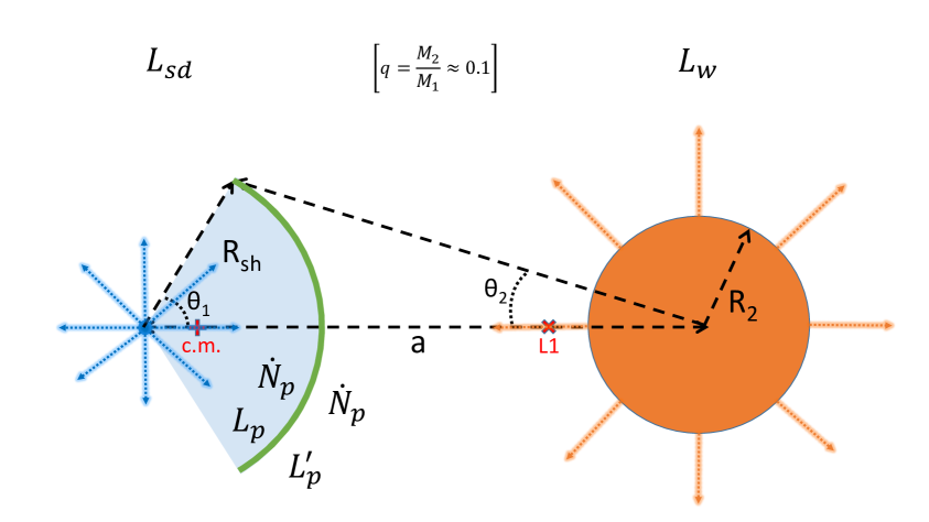
Figure 2: Sketch of the model for reaccelerated $e^{\pm}$ pairs from intrabinary shocks in CBMSPs. The location of the center of mass (c.m.) and inner Lagrangian point (L1) correspond to a mass ratio $q=0.1$.

Companion wind. We approximate $v_{w}$ as the escape velocity from the companion, $v_{w}$=$\sqrt{2GM_{2}/R_{2}}$, where $M_{2}$ and $R_{2}$ are the companion mass and radius, respectively. We assume that the companion fills its Roche lobe, with a volume-equivalent radius $R_{\mathrm{L2}}$. To estimate the mass loss rate in the companion wind, we use an ”evaporative wind” driven by irradiation from the pulsar wind, following the formalism of Ref. [80]. In this scenario, a fraction $f_{w}$ of the irradiating luminosity intercepted by the companion goes into launching a thermal wind, with a kinetic luminosity

$$L_{\mathrm{w}}=\frac{\dot{M}v_{w}^{2}}{2}=f_{w}L_{\mathrm{sd}}\left(\frac{R_{2}}{2a}\right)^{2}.$$ (3.3)

The mass loss rate in the companion wind then becomes

$$\dot{M}_{w}=f_{w}\left(\frac{R_{2}}{4GM_{2}}\right)\left(\frac{R_{2}}{a}\right)^{2}\,.$$ (3.4)

Shock magnetic field and maximal pair energy. We then calculate the strength of the pulsar’s magnetic field at the shock, $B_{\mathrm{sh}}$. We assume that the field is dipolar inside the light cylinder ($\propto 1/r^{3}$) and toroidal outside ($\propto 1/r$) [31]. The synchrotron loss $t_{s}$ and diffusive acceleration $t_{a}$ time scales at the shock depend on $B_{\mathrm{sh}}$ and the energy $E$ of electrons and positrons as [31],

$$t_{s}=200\,\text{s}\left(\frac{\mathrm{G}}{B_{\mathrm{sh}}}\right)^{2}\frac{\mathrm{TeV}}{E},$$ (3.5)

and

$$t_{a}\simeq\frac{E}{ceB_{\mathrm{sh}}}\frac{\xi(\xi+1)}{(\xi-1)}=0.043~{}\text{s}~{}\frac{\xi(\xi+1)}{(\xi-1)}~{}\frac{\mathrm{G}}{B_{\mathrm{sh}}}~{}\frac{E}{\mathrm{TeV}}\,,$$ (3.6)

where the shock compression ratio $\xi$ is $\simeq 4$ for a strong shock. By equating these two time scales, we estimate the maximal or cut-off energy of the pair spectra due to synchrotron losses,

$$E_{\mathrm{cut}}=68~{}\text{TeV}~{}\left(\frac{B_{\mathrm{sh}}}{\text{G}}\right)^{-1/2}~{}\sqrt{\frac{(\xi-1)}{\xi(\xi+1)}}\,.$$ (3.7)

As noted in Ref. [31], $B_{\mathrm{sh}}$ is high so intrabinary shocks in CBMSPs are potentially efficient particle accelerators. Synchrotron losses, however, impose a limit on the maximum energy of electron and positrons and thus on the kinetic power of the outgoing pairs. The closer the shock is to the pulsar, the higher is $B_{\mathrm{sh}}$ and the lower is $E_{\mathrm{cut}}$. For our systems, this limit is in the range $E_{\mathrm{cut}}=(1-10)$ TeV, and the relevant magnetic fields are $\gtrsim 10$ G, as we will show in Section 3.2. The Larmor radius of the accelerated $e^{\pm}$ is $R_{\mathrm{L}}\simeq 3\times 10^{9}\text{cm}~{}(E/\mathrm{TeV})(\mathrm{G}/B)\lesssim 10^{9}\,\text{cm}$, which is in any case more than ten times smaller than the size of the accelerating region ($R_{\mathrm{sh}}\gtrsim 6\times 10^{10}$ cm). Therefore, the pairs can be accelerated to the relevant energies before escaping the shock and the synchrotron limit prevails.

Input pair spectra. The input or “secondary” pairs entering the shock are assumed to have a minimum energy $E_{\min}$ between 1 and 50 GeV. This range is taken from the pair cascade simulations of Harding and Muslimov tailored to MSPs [11], cf. with their Figure 10. The pair spectra they find are relatively soft, $\mathrm{d}N/\mathrm{d}E\propto E^{-\alpha}$ with $\alpha\simeq 3$, with low- and high-energy cutoffs at $E_{\min}=1-50$ GeV and $\sim 1$ TeV, respectively. Because we are mainly interested on the cosmic-ray positron excess seen at Earth well above 20 GeV, we only use this “secondary” component as input for shock acceleration, and neglect the direct contribution to the positron flux at Earth. This direct contribution was deemed negligible by Venter et al. when studying all Galactic MSPs [33].

The total rate of pairs emitted from each polar cap, and the luminosity that these carry, depend mostly on the spin-down luminosity of the pulsar. Using the results of Ref. [11], from their intermediate case with offset polar cap parameter $\varepsilon=0.2$, the total “incoming” pair rate that reaches the shock is

$$\dot{N}_{\mathrm{p}}=2\Omega_{1}\times 8.5\times 10^{33}\,\text{s}^{-1}\left(\frac{L_{\mathrm{sd}}}{10^{35}\,\text{erg\,s}^{-1}}\right)^{0.91}\,,$$ (3.8)

and the total ”incoming” pair luminosity that reaches the shock is

$$L_{\mathrm{p}}=2\Omega_{1}\times 3.2\times 10^{32}\,\text{erg\,s}^{-1}\left(\frac{L_{\mathrm{sd}}}{10^{35}\,\text{erg\,s}^{-1}}\right)^{0.86}\,,$$ (3.9)

both of which we use below to normalize the post-shock or ”tertiary” pair spectrum.

Shock acceleration. At the shock, pairs can gain energy via the so-called Fermi first-order acceleration when travelling back and forth across the termination front [81]. Such “reacceleration” will harden the pair spectrum as compared to the secondary/incoming one, and increase the maximum energy of the tertiary/outgoing pairs. In particular, first-order Fermi acceleration in strong non-relativistic shocks results in a universal spectral energy distribution with power-law index $\simeq 2$ [81]. Although the shock is trans-relativistic, we will assume that a power-law energy distribution with index $\simeq 2$ is a reasonable approximation to the post-shock electron-positron spectrum.

Normalization and energy balance. Using these assumptions, the differential rate of shock accelerated pairs between $E_{\min}$ and $E_{\max}$ is given by

$$Q(E)=\frac{\mathrm{d}N}{\mathrm{d}E\,\mathrm{d}t}=KE^{-2}\,,$$ (3.10)

where $K$ is a normalization constant. This simple analytical model allows us to calculate the integrated tertiary pair rate,

$$\dot{N}^{\prime}_{\mathrm{p}}=\int_{E_{\min}}^{E_{\max}}KE^{-2}\mathrm{d}E=K\left(\frac{1}{E_{\min}}-\frac{1}{E_{\max}}\right)\simeq\frac{K}{E_{\min}},$$ (3.11)

where the last step is valid for $E_{\max}\gg E_{\min}$, and the integrated tertiary pair luminosity,

$$L^{\prime}_{\mathrm{p}}=\int_{E_{\min}}^{E_{\max}}KE^{-1}\mathrm{d}E=K\ln{\frac{E_{\max}}{E_{\min}}}.$$ (3.12)

To normalize the post-shock/tertiary pair spectra, we assume that the number of pairs is conserved,

$$\dot{N}_{\mathrm{p}}=\dot{N}^{\prime}_{\mathrm{p}}\simeq\frac{K}{E_{\min}}\,,$$ (3.13)

and that the maximum integrated pair luminosity is the sum of three terms: i) the incoming/secondary pair luminosity; ii) an additional fraction $\sigma$ of the spin-down luminosity intercepted by the shock, and iii) the kinetic luminosity of the companion’s wind which is intercepted by the shock. That is,

$$L^{\prime}_{\mathrm{p,max}}=L_{\mathrm{p}}+\sigma\Omega_{1}L_{\mathrm{sd}}+\Omega_{2}L_{\mathrm{w}}\,,$$ (3.14)

and the maximum energy allowed by the available luminosity at the shock, Eq. (3.12), becomes

$$E_{\max}=E_{\min}{\mathrm{e}}^{L^{\prime}_{\mathrm{p,max}}/K}\,.$$ (3.15)

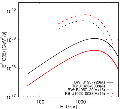
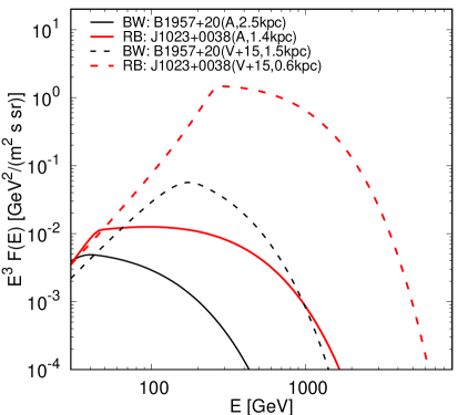
Figure 3: Left: Injected pair spectra from our model A (solid lines) for the prototypical black widow and redback systems B1957+20 and J1023+0038 shown in black and red, respectively, compared with the injected spectra (dashed lines) from Ref. [33] (their case $\varepsilon=0.6,\,\eta_{\mathrm{p,max}}=0.3$). Right: Diffused pair spectra on Earth, for the same two systems. Solid lines show our results with updated distance measurements, dashed lines show previous work from Ref. [33].

We find the last term in Eq. (3.14) negligible in most cases, since $\Omega_{2}L_{\mathrm{w}}$ is more than ten times lower than $L_{\mathrm{p}}$. We see that besides $L_{\mathrm{sd}}$ and geometric factors ($\Omega_{1}$ and $\Omega_{2}$), the additional parameter $\sigma$ determines the luminosity of the outgoing pairs and $E_{\max}$. We have defined $\sigma$ as the fraction of the intercepted spin-down luminosity which is available at the shock as kinetic energy to power Fermi shock acceleration. Thus $\sigma$ reflects the present uncertainty on the magnetic to particle energy content in the pulsar wind (the so-called “sigma problem” mentioned in Section 1, although note that our definition does not necessarily follow previous literature).

The lower of $E_{\max}$ and $E_{\mathrm{cut}}$ gives the true upper limit on the pair energies, which we call $E_{\mathrm{top}}$. Note that we add a high-energy exponential cut-off ${\mathrm{e}}^{-E/E_{\mathrm{top}}}$ to simulate a more physical spectrum. We can finally find the post-shock (tertiary) pair luminosity, taking into account synchrotron losses,

$$L^{\prime}_{\mathrm{p}}=\int_{E_{\min}}^{\infty}KE^{-1}{\mathrm{e}}^{-E/E_{\mathrm{top}}}\mathrm{d}E\,.$$ (3.16)

Summarizing, our model parameters are:

• E_min: The minimum pair energy after shock reacceleration

• $\Omega_{1}$: fraction of the pulsar sky covered by the shock (or fraction of emmitted pairs intercepted by the shock)

• f_w: fraction of the intercepted pulsar wind that launches the companion’s wind

• $\sigma$: fraction of intercepted spin-down luminosity available for shock acceleration

and our main assumptions:

• The post-shock tertiary pair spectrum follows a power law with index $-2$.

• $E_{\min}$ is the same minimum energy of the secondary pairs produced in the pulsar magnetosphere;

• The maximum energy in the post-shock (tertiary) pair spectra ($E_{\mathrm{top}}$) is limited by either the kinetic luminosity available at the shock (which can accelerate pairs up to $E_{\max}$) or by synchrotron losses (which cut off energies above $E_{\mathrm{cut}}$, Eq. (3.7)), i.e., $E_{\mathrm{top}}=\min(E_{\max},E_{\mathrm{cut}})$.

We show in the left panel of Figure 3 the spectra injected into the interstellar medium from our model, for the prototypical black widow and redback systems B1957+20 and J1023+0038. In addition, previous results from Ref. [33] are shown by dashed lines. This comparison shows how the large values of $E_{\min}$ assumed by these authors increase the normalisation of $Q(E)$ by more than an order of magnitude relative to our results. Note that the large values of $E_{\min}$ used in Ref. [33] contradict the basic priniciples of Fermi acceleration: Since at each shock crossing there is a non-zero escape probability, the accelerated energy spectrum has to extend down to the energy with which electrons and positrons are entering the acceleration region. We will model the diffusion of the injected pairs to Earth in Section 4. Here, we show an example for the resulting fluxes in the right panel of Figure 3. In addition to an overall reduction of the flux caused by our normalisation condition relative to the results of Ref. [33], the increased distances of the two sources lead to a suppression of the high-energy tail.

3.2 Model results

We explore three different models (defined by our four parameters as summarized in Table 2) in order to cover the most likely configuration of the intrabinary shock and the injected pair spectra. These are referred to as models A, B and C, in order of decreasing pair rate and luminosity. We refer to the diffuse positron fluxes predicted by these models for the simulated population of CBMSPs as A^′′, B^′′ and C^′′, respectively. When possible, we also compare our results with those for the 24 CBMSPs previously studied in Ref. [33], which we label as V15. Additionally to these samples, we consider also the possibility that in the future a close-by spider at the distance $d=0.5$ kpc will be found. In the case of anisotropic diffusion, the relative position of the sources to the local magnetic field line matters. We distinguish therefore two cases: In case D, we assume that the spider is connected with the Sun by a magnetic field line, $d\simeq d_{\|}$, while in case E the spider is situated orthogonal to the local magnetic field line, $d\simeq d_{\perp}$. Here, $d_{\|}$ and $d_{\perp}$ denote the source distance projected along and perpendicular to the local magnetic field line, respectively.

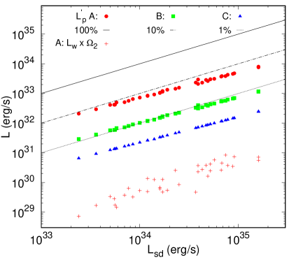
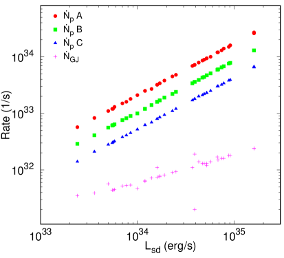
Figure 4: Integrated pair rates (right) and luminosities (left) vs. spin-down luminosity for the 52 CBMSPs studied in this work, from our models A, B and C (red circles, green squares and blue triangles, respectively). Lines on the left panel show 1%, 10% and 100% efficiency in converting spin-down luminosity into pairs reaccelerated at the shock. The companion kinetic luminosity intercepted by the shock (left, red plus signs) and the Goldreich-Julian rate (right, magenta plus signs) are also shown for comparison.

Label	Nr.	Sample	$E_{\mathrm{min}}$	$\Omega_{1}$	$f_{\mathrm{w}}$	$\sigma$
			(GeV)
V15	24	known in 2015	30-1850	1.0	- (0?)	- ?
A′	52	currently known	50	1.0	0.5	0.3
A′′	5000	simulated outside 1 kpc	50	1.0	0.5	0.3
B′	52	currently known.	10	0.5	0.2	0.15
B′′	5000	simulated outside 1 kpc	10	0.5	0.2	0.15
C′	52	currently known.	4	0.25	0.1	0.0
C′′	5000	simulated outside 1 kpc	4	0.25	0.1	0.0
D	1	plane perpendicular	50	1.0	0.5	0.3
E	1	plane parallel	50	1.0	0.5	0.3

Table 2: Models and samples of CBMSPs explored in this work.

Figure 4 shows the luminosities ($L^{\prime}_{\mathrm{p}}$, left) and tertiary (post-shock) pair rates ($\dot{N}_{\mathrm{p}}$, right) for the 52 spiders in our sample, calculated with our models A, B and C. The close to linear dependence on $L_{\mathrm{sd}}$ is readily visible, inherited from the MSP pair cascade simulations (Eqs. (3.8) and (3.9), from [11]). We find that the tertiary pair rates are between 4 and 100 times $\dot{N}_{\mathrm{GJ}}$, while the tertiary pair luminosities are between 0.1% and 10% of the spin-down luminosity $L_{\mathrm{sd}}$. We also find that, as expected and as mentioned in Section 3.1, the contribution of the kinetic luminosity from the companion’s wind $\Omega_{2}L_{\mathrm{w}}$ is negligible, between one and three orders of magnitude lower than $L^{\prime}_{\mathrm{p}}$ (Fig. 4, left).

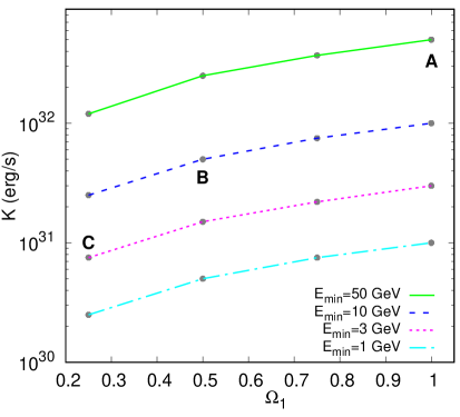
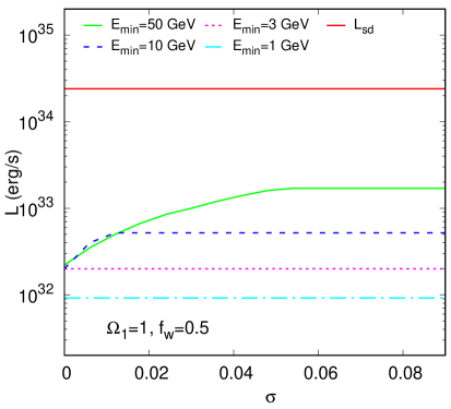
Figure 5: Left: Average normalization of the post-shock pair spectra as a function of $\Omega_{1}$ (fraction of the pulsar sky covered by the shock), for different values of $E_{\min}$. The location of our ABC models is shown with bold letters. Right: Average post-shock pair luminosity as a function of $\sigma$ (fraction of intercepted $L_{\mathrm{sd}}$ that can accelerate pairs), for different values of $E_{\min}$.

The most important parameter in setting the tertiary pair rates and luminosities is the minimum energy of the pairs injected into the shock, $E_{\min}$. Since the integrated rate is dominated by the lowest energies ($Q(E)\propto E^{-2}$), the injected rate and minimum energy together determine the normalization $K$, cf. with Eq. (3.13). Thus the assumed $E_{\min}$ is the key for a correct normalization of the injected and observed pair fluxes. This is shown in Figure 5, where $K$ and $L^{\prime}_{\mathrm{p}}$ are plotted as a function of $\Omega_{1}$ and $\sigma$, respectively, for different values of $E_{\min}$ (this and the subsequent Figure 6 show average values in our sample of 52 CBMSPs). We see that, depending on mostly $E_{\min}$ but also $\Omega_{1}$, $K$ can vary by a bit more than two orders of magnitude.

In general, the outgoing pair luminosity $L^{\prime}_{\mathrm{p}}$ is limited by synchrotron losses and is at most 10% of $L_{\mathrm{sd}}$ (for $E_{\min}=50$ GeV, our model A; Figs. 4 and 5). It is interesting to note that $L^{\prime}_{\mathrm{p}}$ saturates at 10% of $L^{\prime}_{\mathrm{sd}}$ for $\sigma\gtrsim 0.05$, as shown in the right panel of Figure 5. Note also that the pairs injected into the shock carry at most 1% of $L_{\mathrm{sd}}$ (cf. with Eq. (3.9) of Ref. [11]). Previous work [33] assumed that this efficiency $\eta=L^{\prime}_{\mathrm{p}}/L_{\mathrm{sd}}$ can be up to 30%, and that pairs always reach the synchrotron cut-off energy $E_{\mathrm{cut}}$. This leads to artificially high values for both $K$ and $E_{\min}$, as can be seen in the left panel of Figure 3.

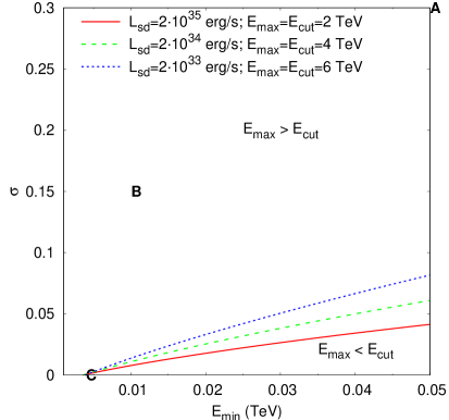
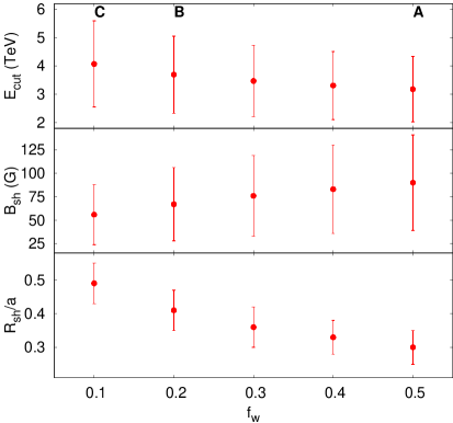
Figure 6: Left: Boundaries between the synchrotron-limited ($E_{\max}>E_{\mathrm{cut}}=E_{\mathrm{top}}$) and the power-limited ($E_{\mathrm{cut}}>E_{\mathrm{\max}}=E_{\mathrm{top}}$) regimes, for different values of $E_{\mathrm{cut}}$ and $L_{\mathrm{sd}}$ (as indicated). Right (from bottom up): Average and standard deviation of the shock radius (in units of the orbital separation, $a$), magnetic field and synchrotron cut-off energy as a function of the companion wind launching efficiency, $f_{\mathrm{w}}$. In both cases the location of our ABC models is shown with bold letters.

Our model reveals two distinct regimes of intrabinary shock acceleration, depending on the parameters $E_{\min}$ and $\sigma$, as shown in the left panel of Figure 6. In what we call the power-limited regime (model C), the maximum pair energy is not set by synchrotron losses but rather limited by the available kinetic power at the shock, that is, $E_{\mathrm{top}}=E_{\max}<E_{\mathrm{cut}}$. This regime occurs only for $E_{\min}\gtrsim 4$ GeV and $\sigma\lesssim 0.05$, with the exact boundaries shown in Figure 6. Instead, in the synchrotron-limited regime (models A and B), there is abundant kinetic power at the shock to power reacceleration (compared to $K$, cf. Eq. 3.15) so that $E_{\max}$ is high. This is the more common case where the maximum pair energy is set by synchrotron losses, i.e., $E_{\mathrm{top}}=E_{\mathrm{cut}}<E_{\max}$.

Previous work assumed that all pairs created in the pulsar magnetosphere can reach the shock and be reaccelerated [33]. Because this fraction of pairs intercepted by the shock is not tightly constrained, we conservatively explore in this work the range $\Omega_{1}=[0.25-1.0]$, which corresponds to opening angles $\vartheta_{1}=[60^{\circ}-180^{\circ}]$. Varying these parameters changes $\dot{N}_{\mathrm{p}}$ and $L^{\prime}_{\mathrm{p}}$ by a factor four, since the predicted rates are proportional to $\Omega_{1}$. More detailed models of the pressure balance between the pulsar wind and the companion star magnetosphere/wind show more complex “bow” shapes for the intrabinary shock, but a similar range for $\vartheta_{1}$ and $\Omega_{1}$ [82, 79, 83].

We find that the companion wind has no strong impact on the pair spectral parameters, with our main assumption of an irradiation driven wind (Sec. 3.1). The range $f_{\mathrm{w}}=[0.1-0.5]$ that we explore in this work yields relatively high mass loss rates for the companion, of the order $10^{15}$–$10^{17}$ g/s. We find that the shock radius is anti-correlated with the companion wind parameter $f_{\mathrm{w}}$, as shown in Figure 6: The stronger the companion wind is, the closer the shock gets to the pulsar. The corresponding magnetic field at the shock, $B_{\mathrm{sh}}$, is in the 5–240 G range for our ABC models (Sec. A) and shows a weak dependence on the companion wind parameter $f_{\mathrm{w}}$ (Figure 6). These values agree with the available observational constraints on the magnetic field at the intrabinary shock [84, 85]. The synchrotron cut-off energy $E_{\mathrm{cut}}$, which is always in the range 2–10 TeV, also shows a weak dependence on $f_{\mathrm{w}}$.

4 Galactic transport with regular and turbulent fields

The transport equation for the differential number density $n(\boldsymbol{x},t,E)$ of positrons including energy losses $b(E,t)$ is given by

$$\frac{\partial n}{\partial t}-\boldsymbol{\nabla}_{i}D_{ij}\boldsymbol{\nabla}_{j}n-\frac{\partial}{\partial E}(bn)=Q.$$ (4.1)

In the presence of a regular, uniform magnetic field, the diffusion tensor $D_{ij}$ can be written as

$$D_{ij}=D_{\|}e_{i}e_{j}+D_{\perp}(\delta_{ij}-e_{i}e_{j})\,.$$ (4.2)

Here, $\boldsymbol{e}$ is a unit vector in the direction of the regular magnetic field, while the diagonal elements of the diffusion tensor describe diffusion along ($D_{\parallel}$) and perpendicular ($D_{\perp}$) to the regular field. In Ref. [86], these diffusion coefficients were calculated as function of the ratio of the strength of the regular and the turbulent field, $\eta=B_{\rm rms}/B_{0}$. Since charged particles can move freely along the direction of the regular field, while they gyrate along the line in the perpendicular directions, there is a strong ordering of the two diffusion coefficients, $D_{\parallel}\gg D_{\perp}$, for $\eta\ll 10$. Comparing then the resulting grammage crossed by CRs to measurements, the authors of Ref. [86] determined a range of allowed values for the diffusion parameters. In particular, they argued that in the Jansen-Farrar model [87] for the regular Galactic magnetic field, a value of $\eta\approx 0.25$ is consistent with the average angle of $20^{\circ}$ between magnetic field lines and the Galactic plane. The need for anisotropic CR diffusion was previously stressed in Refs. [88, 89].

The solution of Eq. (4.1) can be found either using the Green function method [90] or by Fourier transforming its spatial part [91], introducing the Syrovatskii variables

$$\lambda_{i}^{2}(E,E_{g})=\int_{t_{g}}^{t}\mathrm{d}t^{\prime}\,D_{i}(E(t^{\prime}))=\int_{E}^{E_{g}}\mathrm{d}E^{\prime}\,\frac{D_{i}(E^{\prime})}{b(E^{\prime})}$$ (4.3)

with $i=\{\perp,\|\}$. These new variables correspond to the squared distance traveled by a particle perpendicular and parallel to the magnetic field line, while its energy diminishes from $E_{g}$ to $E$. Assuming for the energy scaling of the diffusion coefficient a power law, $D_{i}=D_{0,i}(E/E_{0})^{\delta}$, and using quadratic energy losses $b=-\mathrm{d}E/\mathrm{d}t=\beta E^{2}$ typical for Thomson and synchrotron losses, one can find a closed expression for the Syrovatskii variable,

$$\lambda_{i}^{2}(E,E^{\prime})=\frac{D_{0,i}}{(\delta-1)\beta E}\>\left(\frac{E}{E_{0}}\right)^{\delta}\left[\left(\frac{E^{\prime}}{E}\right)^{\delta-1}-1\right].$$ (4.4)

The case of anisotropic diffusion can be reduced to isotropic diffusion, recalling that the isotropic Green function factorizes in Cartesian coordinates. Alternatively, one can first diagonalise $D_{ij}$ by a rotation, and then perform a scale transformation. In either case, one finds for the case of a single source at the distance $r$,

$$n(\boldsymbol{r})=\int\mathrm{d}E^{\prime}\,\frac{Q(E^{\prime})}{b(E)}\>\frac{\exp\left(-\frac{\boldsymbol{r}_{\perp}^{2}}{4\lambda_{\perp}^{2}}\right)\exp\left(-\frac{\boldsymbol{r}_{\|}^{2}}{4\lambda_{\|}^{2}}\right)}{\left(4\pi\right)^{3/2}\lambda_{\perp}^{2}\lambda_{\|}}.$$ (4.5)

We calculate $r_{\perp}$ and $r_{\|}$ by projecting $\boldsymbol{r}$ on the unit vector along the magnetic field line going through the source. The direction of the magnetic field line is determined in turn by using the spiral field of the Jansen-Farrar model [87] for its $x$-$y$ components and adding an $X$ field-like component with angle $\vartheta=20^{\circ}$ to the Galactic plane. While this toy model neglects, e.g., the increase of $|\vartheta|$ for increasing $z$, it captures the main differences to the usually considered case of isotropic diffusion. The latter is obtained by setting $D_{\perp,0}=D_{\|,0}=D_{0}$ in Eq. (4.4).

Finally, we note that the solution (4.5) is valid in $\hbox{$R$}^{3}$. In order to take into account the finite vertical extension $H$ of the Galactic CR halo, $H\simeq 5$ kpc, and the resulting escape of CRs, we multiply therefore the integrand by the function $\exp(-\lambda_{\|}\sin\vartheta/H)$. For the case of anisotropic diffusion, we set $D_{\perp,0}=2\times 10^{26}$ cm²/s and $D_{\|,0}=5\times 10^{28}$ cm²/s at $E_{0}=5$ GeV, while we use $D_{0}=3\times 10^{28}$ cm²/s for isotropic diffusion [86]. Moreover, we assume Kolmogorov diffusion, $\delta=1/3$, motivated by the B/C measurements of AMS-02 [92] and use $\beta=4\times 10^{-17}$ GeV/s.

5 Diffuse positron flux from spiders

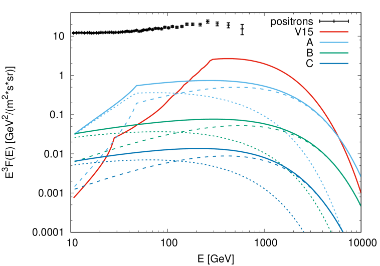
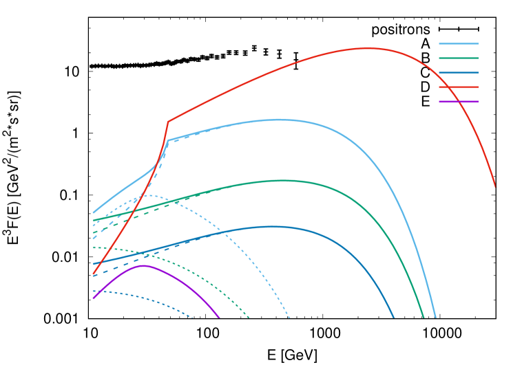
Figure 7: Positron fluxes on Earth after isotropic diffusion from our ABC models. Dashed and dotted lines show the contribution from the currently known and simulated population of CBMSPs, respectively, and solid lines show total flux. Black error bars show the AMS-02 data and the red line compares to previous work (V15, [33]; see Table 2 and Section 5).

Figure 8: Positron fluxes on Earth after anisotropic diffusion from our ABCDE models. Lines labelled D and E show the contribution from one nearby CBMSP on the Galactic plane from a direction which is aligned and misaligned with the regular Galactic magnetic field, respectively (other lines and symbols as in Fig. 8; see Table 2 and Section 5).

As a first step, we compare the diffuse positron flux reported by Venter et al. in Ref. [33] (their Figure 8, cyan lines) with the diffuse flux that we calculate from their source sample and using their distances (the 24 spiders known in 2015; red line in Figure 8). We use for the purpose of this comparison their injected source spectra for $\varepsilon=0.6$ and $\eta_{\mathrm{p,max}}=0.3$, even if we have argued that they overestimate both $K$ and $E_{\min}$. This serves as a cross-check on the diffuse positron fluxes expected from CBMSPs on Earth (with the same value of $D_{0}=3\times 10^{28}$ cm²/s). We reproduce the same shape of the diffuse positron spectrum from those 24 spiders, with the same break at 300 GeV (due to source 1 in Table 1, which they placed at an underestimated distance). Note, however, that the spider spectra calculated by Venter et al. miss the low-energy tail visible in Figure 8 which is caused by the energy losses of propagating positrons. As a result, their fluxes at 300 GeV are about a factor three higher. Additionally, the different energy scaling of the diffusion coefficient ($\delta=1/3$ versus $\delta=0.6$) leads to minor differences in the predicted fluxes.

Figure 8 shows the diffuse positron fluxes on Earth calculated in the isotropic approximation from our source models ABC (Table 2), compared to the AMS-02 data. We show the positron spectra from the currently known population of 52 CBMSPs with dashed lines (A^′, B^′ and C^′ in Table 2), and those of the simulated population of 5000 CBMSPs with dotted lines (A^′′, B^′′ and C^′′; see Section 2.2 for details). Together, they approximate the total diffuse positron flux on Earth from spiders in our Galaxy (A, B and C; solid lines in Figure 8). At 100 GeV, our model predicts a total diffuse positron flux between 25 (A) and 1000 times (C) lower than that measured by AMS-02. We conclude that the diffuse positron flux that our model predicts from the total Galactic population of CBMSPs is only a minor contribution to the observed flux.

We find that the simulated population of 5000 CBMSPs (dotted lines in Fig. 8) contributes with about the same positron flux at 100 GeV as the currently known population (dashed lines). Furthermore, the positron flux from spiders after isotropic diffusion is suppressed above a few TeV. As expected, we find that the closest spiders dominate the positron flux: the five spiders with the highest positron flux (three BWs and two RBs) are all within less than 1 kpc from Earth. We refer to Appendix A for further details on individual sources. The contribution from the simulated population is softer, i.e., its high energy flux is suppressed relative to the one from the currently known spiders, because of more severe energy losses.

Our results for the diffuse positron flux on Earth with anisotropic transport due to the ordered Galactic magnetic field are shown in Figure 8. We find that the total fluxes and spectra from CBMSPs are not drastically modified, but in this case they are clearly dominated by the currently known population of spiders (dashed lines in Fig. 8). The simulated Galactic population of 5000 CBMSPs contributes with less than 10% of the flux at 100 GeV in this case. This can be understood as follows; for the chosen parameters of $D_{\|}$ and $D_{\perp}$, the effective volume filled by positrons emitted by a single source is reduced by a factor $\simeq 100$ [86]. Therefore the number of sources contributing to the locally measured CR flux is correspondingly reduced and, as a result, one expects the local flux even in the 100 GeV range to be dominated by few local sources [93, 94]. Correspondingly, the flux of sources in the simulated population—which are at larger distances—is suppressed. Note, however, that the uncertainties in current models of the Galactic magnetic field [95] are too large to identify the dominating sources.

Finally, we consider the flux from two nearby and yet undiscovered spiders near the Galactic plane. In Section 2.2, we have estimated that 2–3 such spiders may be ”hidden” in the Solar neighborhood and near the Galactic plane ($|\ell|<5^{\circ}$ and $d<1$ kpc). We show in Figure 8 their contribution to the local diffuse positron flux, assuming that their line of sight to Earth is either parallel or perpendicular to the ordered Galactic magnetic field. The first case (labelled D) represents the effects of anisotropic diffusion in a favorable orientation (along magnetic field lines) while the second case (E) shows the least favorable diffusion direction (across magnetic field lines). The difference in flux is drastic, three orders of magnitude at 100 GeV (Figure 8), although the assumed distance (0.5 kpc) and injected spectrum (average of A) are exactly the same.

The positron spectrum from our model D reaches the diffuse flux measured by AMS-02 at 600 GeV. Taken at face value, this case predicts a second peak in the positron flux at 2–6 TeV. In Fig. 9, we compare additionally the combined electron and positron flux from the same source to measurements from CALET [96], DAMPE [97], Fermi-LAT [98] and H.E.S.S. [99]; the predicted flux from such a source agrees with the existing observations in the 1–10 TeV range. Note, however, that the result of case D might be overly optimistic; since the Sun is located inside the Local Bubble, the magnetic field in the bubble wall will act as a shield, reducing the CR flux. In Ref. [100], it was shown that this reduction is rather severe in the case of a young source like Vela. For continuous sources like spiders, the flux suppression due to the Local Bubble should be smaller. Detailed calculations of positron propagation taking into account the local magnetic field structure would be needed to quantify properly this effect. We conclude that nearby spiders close to the Galactic plane may give a substantial contribution both to the observed flux of positrons above a few hundred GeV and the combined flux of electrons and positrons above TeV energies, if their line-of-sight to Earth is aligned with the ordered Galactic magnetic field.

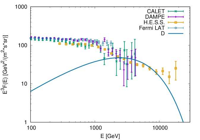
Figure 9: Measurements of the diffuse flux of electrons and positrons on Earth from CALET, DAMPE, Fermi-LAT and H.E.S.S. compared to the flux from our case D.

6 Summary and conclusions

We have determined the Galactic scale height of spiders as $z_{\mathrm{e}}=0.4\pm 0.1$ kpc, and found that the observed population of spiders is strongly biased against small Galactic heights, $|z|<0.5$ kpc (Section 2.1). We attribute this to selection effects of previous searches, which have avoided low Galactic latitudes to minimize gamma-ray background and interstellar absorption. Increasing the sensitivity of CBMSP searches (e.g. with the latest Fermi-LAT source catalog) and pushing them to lower Galactic latitudes ($|\ell|\raise 1.29167pt\hbox{$\;<$\kern-7.5pt\raise-4.73611pt\hbox{$\sim\;$}}1^{\circ}-5^{\circ}$) will allow us to find more nearby spiders, some of which may be particularly important in terms of cosmic-ray positrons.

We have presented in Section 3 a simple physical model for the fluxes and spectra of “tertiary” pairs, after being reaccelerated at the intrabinary shock in CBMSPs. We have found that the normalization of such tertiary pair spectra depends mainly on the input rate as well as the minimum energy of the pairs ($K\simeq\dot{N}^{\prime}_{\mathrm{p}}~{}E_{\min}$). Taking $E_{\min}$ and $\dot{N}$ from current models, we find that each spider injects between $10^{32}$ and a few times $10^{34}$ pairs/s into the interstellar medium, with energies up to 10 TeV. We also pointed out that, no matter how much kinetic energy is available at the shock for reacceleration, after taking into account synchrotron losses the energy output in pairs is limited to 10% of $L_{\mathrm{sd}}$.

Finally, we found in Section 5 that the contribution from spiders to the diffuse positron flux on Earth is less than 5% of the diffuse flux measured by AMS-02. As expected, the five spiders that produce the highest positron fluxes are all within 1 kpc (App. A). We also find that the effects of anisotropic diffusion modify strongly the contribution from individual spiders. Accurate distances to the nearest sources (e.g. from Gaia’s final data) and good knowledge of the local structure of the Galactic magnetic field will narrow down the predicted range of positron fluxes. In any case, even with the moderate 10% efficiency from our source injection model, we conclude that one single nearby CBMSP at 0.5 kpc on the Galactic plane can contribute significantly to the positron flux at energies above a few hundred GeV and to the combined electron and positron flux above $\simeq$ 1 TeV, if it is favorably positioned with respect to the ordered Galactic field.

Appendix A Injected pair spectra

We give in this Appendix the model parameters for our three models (Tables 3, 4 and  5), applied to each of the 52 known CBMSPs (Section 2.1). Figure 10 shows the diffuse positron fluxes from our model A for each of the 52 individual CBMSPs. The top 5 sources in terms of flux at 1 TeV are source 31, 51, 50, 8 and 12 in Table 1, at distances of 0.7, 0.6, 0.5, 0.75 and 0.9 kpc, respectively. The two faintest sources are 46 and 41, at 4.6 and 6.1 kpc from Earth, respectively. The ”bump” at 3 TeV in our isotropic diffuse spectra (models A and B in Figure 8) is due to source 12, which has the highest $E_{\mathrm{top}}$ (Figure 10 and Tables 3 and 4). At energies lower than E_min the diffuse positron spectra show an artificial sharp decrease in flux, which is due to our assumed step-like low energy cut-off in the injected spectra.

ID	Rsh/a	Bsh	Etop	$\Omega_{2}$	Lw/1032	K/1032	$L^{\prime}_{\mathrm{p}}$/1032	$\dot{N}_{\mathrm{p}}$/1033
-	-	$\mathrm{G}$	$\mathrm{TeV}$	-	$\mathrm{erg\,s^{-1}}$	$\mathrm{erg\,s^{-1}}$	$\mathrm{erg\,s^{-1}}$	s-1
1	0.27	132	2.3	0.018	3.2	8.2	27	10
2	0.25	54	3.6	0.016	0.85	2	7.4	2.5
3	0.26	135	2.3	0.018	4.1	12	41	16
4	0.22	47	3.8	0.012	1.2	3.7	14	4.6
5	0.25	91	2.8	0.016	2.8	9.6	33	12
6	0.29	53	3.6	0.022	0.29	1.3	5	1.6
7	0.27	66	3.2	0.019	0.66	2.2	8	2.7
8	0.23	66	3.2	0.013	2.9	6.9	25	8.6
9	0.25	91	2.8	0.016	2.6	7.5	26	9.4
10	0.31	104	2.6	0.025	0.62	3.7	13	4.6
11	0.28	64	3.3	0.02	0.63	2.7	9.9	3.4
12	0.22	10	8.2	0.012	3.1	5.8	27	7.2
13	0.27	166	2	0.019	4.4	10	33	13
14	0.26	88	2.8	0.017	1.5	3.6	12	4.5
15	0.21	44	3.9	0.012	1.7	3.7	14	4.6
16	0.20	51	3.7	0.01	2.9	3.7	14	4.6
17	0.29	127	2.3	0.022	1.2	3.7	12	4.6
18	0.27	92	2.7	0.019	1.2	3.7	13	4.6
19	0.25	66	3.2	0.016	1.2	3.7	14	4.6
20	0.24	28	5	0.014	0.24	0.89	3.6	1.1
21	0.27	92	2.7	0.018	1.2	3.9	13	4.8
22	0.26	78	3	0.017	1.2	3.7	13	4.6
23	0.31	129	2.3	0.024	2.3	21	69	26
24	0.31	36	4.4	0.025	0.13	1.4	5.7	1.8
25	0.35	52	3.7	0.031	0.091	0.97	3.7	1.2
26	0.35	70	3.1	0.032	0.19	2.6	9.3	3.2
27	0.33	81	2.9	0.027	0.37	3.7	13	4.6
28	0.41	58	3.4	0.044	0.039	0.99	3.7	1.2
29	0.32	166	2	0.027	0.33	3.7	12	4.6
30	0.32	84	2.9	0.026	0.26	2.6	9	3.2
31	0.32	112	2.5	0.026	1	9.5	32	12
32	0.41	177	2	0.044	0.37	7.1	22	8.9
33	0.40	58	3.4	0.043	0.11	5.5	20	6.9
34	0.34	147	2.2	0.029	1.2	12	39	15
35	0.36	66	3.2	0.033	0.15	2	7.2	2.5
36	0.34	187	1.9	0.03	0.91	6.3	20	7.9
37	0.29	108	2.5	0.022	1.7	11	37	14
38	0.30	17	6.5	0.023	0.063	1	4.4	1.3
39	0.31	80	2.9	0.024	0.36	3.7	13	4.6
40	0.32	192	1.9	0.026	0.88	5.8	18	7.2
41	0.37	31	4.7	0.036	0.02	0.46	1.8	0.57
42	0.35	94	2.7	0.031	0.34	3.7	13	4.6
43	0.35	64	3.3	0.031	0.12	1.2	4.4	1.5
44	0.33	50	3.7	0.028	0.19	1.7	6.3	2.1
45	0.34	171	2	0.03	0.45	3.7	12	4.6
46	0.34	39	4.2	0.031	0.054	0.66	2.6	0.83
47	0.35	237	1.7	0.031	2.3	21	64	27
48	0.32	41	4.1	0.026	0.21	3	12	3.8
49	0.31	38	4.2	0.025	0.19	2.7	11	3.4
50	0.36	84	2.9	0.034	0.25	3.9	14	4.8
51	0.31	96	2.7	0.025	0.99	7.5	26	9.4
52	0.38	174	2	0.038	0.34	3.7	12	4.6

Table 3: Companion wind, intrabinary shock and pair spectral parameters for the 52 spiders, from our model A.

ID	Rsh/a	Bsh	Etop	$\Omega_{2}$	Lw/1032	K/1032	$L^{\prime}_{\mathrm{p}}$/1032	$\dot{N}_{\mathrm{p}}$/1033
-	-	$\mathrm{G}$	$\mathrm{TeV}$	-	$\mathrm{erg\,s^{-1}}$	$\mathrm{erg\,s^{-1}}$	$\mathrm{erg\,s^{-1}}$	s-1
1	0.37	97	2.7	0.035	1.3	0.82	4.2	5.1
2	0.35	39	4.2	0.031	0.34	0.2	1.1	1.2
3	0.36	98	2.7	0.034	1.7	1.2	6.4	7.8
4	0.31	34	4.5	0.024	0.47	0.37	2.1	2.3
5	0.35	66	3.2	0.031	1.1	0.96	5.2	6
6	0.39	39	4.2	0.04	0.11	0.13	0.75	0.82
7	0.37	48	3.8	0.035	0.27	0.22	1.2	1.4
8	0.32	47	3.8	0.026	1.2	0.69	3.8	4.3
9	0.35	66	3.2	0.031	1	0.75	4	4.7
10	0.42	78	3	0.046	0.25	0.37	2	2.3
11	0.38	47	3.8	0.037	0.25	0.27	1.5	1.7
12	0.31	7	9.7	0.024	1.2	0.58	4	3.6
13	0.37	121	2.4	0.035	1.7	1	5.2	6.5
14	0.36	64	3.3	0.033	0.6	0.36	1.9	2.2
15	0.30	32	4.7	0.023	0.68	0.37	2.2	2.3
16	0.29	36	4.4	0.021	1.1	0.37	2.1	2.3
17	0.39	94	2.7	0.04	0.47	0.37	1.9	2.3
18	0.37	67	3.2	0.035	0.47	0.37	2	2.3
19	0.35	48	3.8	0.031	0.47	0.37	2.1	2.3
20	0.33	20	5.8	0.028	0.095	0.089	0.55	0.56
21	0.37	67	3.2	0.035	0.49	0.39	2.1	2.4
22	0.36	57	3.5	0.033	0.47	0.37	2	2.3
23	0.41	96	2.7	0.044	0.9	2.1	11	13
24	0.42	27	5.1	0.046	0.054	0.14	0.86	0.9
25	0.46	39	4.2	0.056	0.036	0.097	0.55	0.61
26	0.46	53	3.6	0.057	0.076	0.26	1.4	1.6
27	0.43	61	3.4	0.049	0.15	0.37	2	2.3
28	0.53	46	3.9	0.075	0.016	0.099	0.55	0.62
29	0.43	125	2.4	0.048	0.13	0.37	1.9	2.3
30	0.42	63	3.3	0.047	0.11	0.26	1.4	1.6
31	0.42	84	2.9	0.047	0.41	0.95	5	5.9
32	0.52	138	2.2	0.073	0.15	0.71	3.5	4.4
33	0.52	46	3.9	0.072	0.044	0.55	3.1	3.4
34	0.44	111	2.5	0.052	0.48	1.2	6.2	7.6
35	0.47	50	3.7	0.058	0.061	0.2	1.1	1.2
36	0.45	141	2.2	0.053	0.36	0.63	3.1	3.9
37	0.40	80	2.9	0.041	0.66	1.1	5.7	6.8
38	0.40	12	7.5	0.042	0.025	0.1	0.66	0.64
39	0.41	59	3.4	0.045	0.14	0.37	2	2.3
40	0.42	144	2.2	0.047	0.35	0.58	2.8	3.6
41	0.49	24	5.4	0.063	0.0079	0.046	0.27	0.29
42	0.46	71	3.1	0.055	0.14	0.37	2	2.3
43	0.46	48	3.8	0.055	0.049	0.12	0.67	0.76
44	0.44	38	4.3	0.051	0.078	0.17	0.96	1
45	0.45	130	2.3	0.053	0.18	0.37	1.9	2.3
46	0.45	30	4.8	0.054	0.022	0.066	0.39	0.41
47	0.46	180	2	0.055	0.9	2.1	10	13
48	0.42	31	4.7	0.047	0.083	0.3	1.8	1.9
49	0.42	29	4.9	0.046	0.077	0.27	1.6	1.7
50	0.47	64	3.3	0.06	0.099	0.39	2.1	2.4
51	0.42	72	3.1	0.046	0.4	0.75	4	4.7
52	0.50	134	2.3	0.066	0.14	0.37	1.8	2.3

Table 4: Companion wind, intrabinary shock and pair spectral parameters for the 52 spiders, from our model B.

ID	Rsh/a	Bsh	Etop	$\Omega_{2}$	Lw/1032	K/1032	$L^{\prime}_{\mathrm{p}}$/1032	$\dot{N}_{\mathrm{p}}$/1033
-	-	$\mathrm{G}$	$\mathrm{TeV}$	-	$\mathrm{erg\,s^{-1}}$	$\mathrm{erg\,s^{-1}}$	$\mathrm{erg\,s^{-1}}$	s-1
1	0.45	79	1.7	0.053	0.64	0.16	0.93	2.5
2	0.43	32	2.7	0.048	0.17	0.04	0.25	0.62
3	0.44	80	1.5	0.052	0.83	0.25	1.4	3.9
4	0.39	27	2.2	0.038	0.24	0.074	0.45	1.2
5	0.43	53	1.6	0.049	0.56	0.19	1.1	3
6	0.48	32	3.2	0.061	0.057	0.026	0.17	0.41
7	0.45	39	2.6	0.054	0.13	0.044	0.28	0.69
8	0.40	38	1.8	0.041	0.58	0.14	0.79	2.1
9	0.43	53	1.7	0.048	0.51	0.15	0.86	2.3
10	0.50	64	2.2	0.068	0.12	0.074	0.45	1.2
11	0.46	38	2.5	0.057	0.13	0.054	0.34	0.85
12	0.38	6	1.9	0.038	0.62	0.12	0.67	1.8
13	0.45	99	1.6	0.054	0.87	0.21	1.2	3.2
14	0.44	52	2.2	0.051	0.3	0.072	0.43	1.1
15	0.38	25	2.2	0.036	0.34	0.074	0.45	1.2
16	0.36	28	2.2	0.033	0.57	0.074	0.45	1.2
17	0.48	77	2.2	0.061	0.24	0.074	0.45	1.2
18	0.45	55	2.2	0.054	0.24	0.074	0.45	1.2
19	0.43	39	2.2	0.048	0.24	0.074	0.45	1.2
20	0.41	16	3.7	0.043	0.047	0.018	0.12	0.28
21	0.45	55	2.2	0.053	0.25	0.077	0.46	1.2
22	0.44	46	2.2	0.051	0.24	0.074	0.45	1.2
23	0.50	80	1.2	0.066	0.45	0.42	2.2	6.5
24	0.50	22	3.1	0.068	0.027	0.029	0.19	0.45
25	0.54	33	3.6	0.081	0.018	0.019	0.13	0.3
26	0.55	45	2.5	0.083	0.038	0.051	0.32	0.8
27	0.52	51	2.2	0.073	0.074	0.074	0.45	1.2
28	0.61	39	3.5	0.1	0.0078	0.02	0.13	0.31
29	0.51	104	2.2	0.071	0.066	0.074	0.45	1.2
30	0.51	52	2.5	0.07	0.053	0.051	0.32	0.8
31	0.51	70	1.6	0.069	0.21	0.19	1.1	3
32	0.61	119	1.8	0.1	0.074	0.14	0.82	2.2
33	0.60	39	1.9	0.1	0.022	0.11	0.65	1.7
34	0.53	93	1.5	0.076	0.24	0.24	1.3	3.8
35	0.55	42	2.7	0.083	0.031	0.04	0.25	0.62
36	0.53	118	1.8	0.077	0.18	0.13	0.73	2
37	0.48	66	1.5	0.062	0.33	0.22	1.2	3.4
38	0.49	10	3.5	0.063	0.013	0.02	0.14	0.32
39	0.50	49	2.2	0.067	0.072	0.074	0.45	1.2
40	0.51	120	1.9	0.07	0.18	0.12	0.67	1.8
41	0.57	20	4.7	0.09	0.0039	0.0091	0.066	0.14
42	0.54	60	2.2	0.08	0.068	0.074	0.45	1.2
43	0.54	41	3.3	0.08	0.025	0.024	0.16	0.38
44	0.53	32	2.9	0.075	0.039	0.034	0.22	0.52
45	0.53	109	2.2	0.077	0.09	0.074	0.45	1.2
46	0.54	25	4.1	0.079	0.011	0.013	0.092	0.21
47	0.54	151	1.2	0.08	0.45	0.43	2.3	6.7
48	0.51	25	2.4	0.07	0.041	0.06	0.37	0.94
49	0.51	24	2.5	0.069	0.039	0.054	0.34	0.85
50	0.56	54	2.2	0.086	0.049	0.077	0.46	1.2
51	0.50	59	1.7	0.068	0.2	0.15	0.86	2.3
52	0.58	115	2.2	0.093	0.068	0.074	0.45	1.2

Table 5: Companion wind, intrabinary shock and pair spectral parameters for the 52 spiders, from our model C.

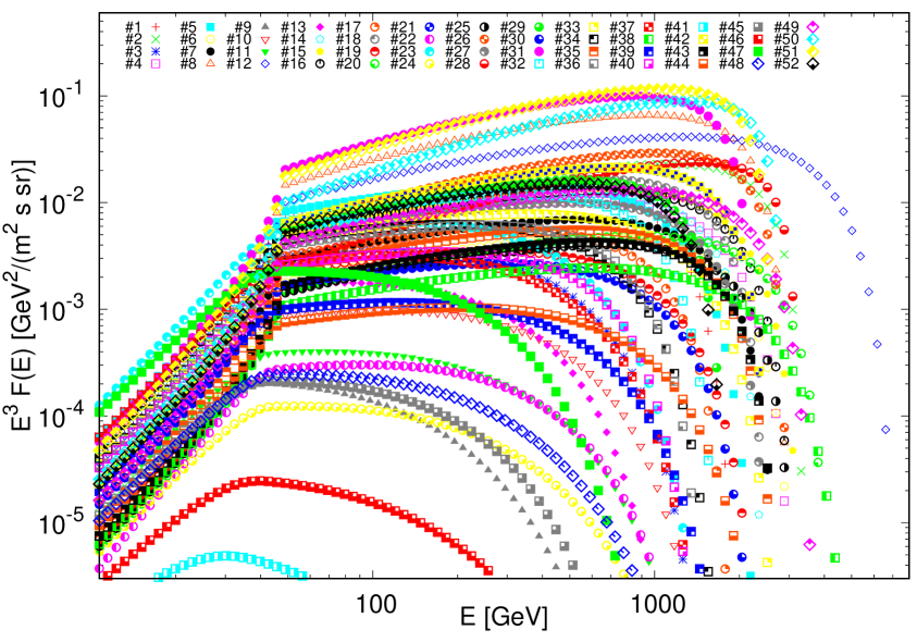
Figure 10: Diffuse positron fluxes on Earth for all 52 known CBMSPs, from our model A.

References

- [1] M. Kachelrieß and D. V. Semikoz, Cosmic ray models, Progress in Particle and Nuclear Physics 109 (2019) 103710 [1904.08160].
- [2] P. D. Serpico, Astrophysical models for the origin of the positron “excess”, Astroparticle Physics 39 (2012) 2 [1108.4827].
- [3] PAMELA collaboration, An anomalous positron abundance in cosmic rays with energies 1.5-100 GeV, Nature 458 (2009) 607 [0810.4995].
- [4] PAMELA collaboration, PAMELA results on the cosmic-ray antiproton flux from 60 MeV to 180 GeV in kinetic energy, Phys. Rev. Lett. 105 (2010) 121101 [1007.0821].
- [5] AMS collaboration, Electron and Positron Fluxes in Primary Cosmic Rays Measured with the Alpha Magnetic Spectrometer on the International Space Station, Phys. Rev. Lett. 113 (2014) 121102.
- [6] M. Aguilar et al., Towards Understanding the Origin of Cosmic-Ray Positrons, Phys. Rev. Lett. 122 (2019) 041102.
- [7] A. K. Harding and R. Ramaty, The Pulsar Contribution to Galactic Cosmic Ray Positrons, International Cosmic Ray Conference 2 (1987) 92.
- [8] A. Boulares, The nature of the cosmic-ray electron spectrum, and supernova remnant contributions, Astrophys. J. 342 (1989) 807.
- [9] P. Goldreich and W. H. Julian, Pulsar Electrodynamics, Astrophys. J. 157 (1969) 869.
- [10] J. G. Kirk, Y. Lyubarsky and J. Petri, The Theory of Pulsar Winds and Nebulae, in Astrophysics and Space Science Library, W. Becker, ed., vol. 357 of Astrophysics and Space Science Library, p. 421, (2009), DOI.
- [11] A. K. Harding and A. G. Muslimov, Pulsar Pair Cascades in Magnetic Fields with Offset Polar Caps, Astrophys. J. 743 (2011) 181 [1111.1668].
- [12] J. Arons and M. Tavani, Relativistic particle acceleration in plerions, Astrophys. J. Suppl. 90 (1994) 797.
- [13] S. V. Bogovalov and F. A. Aharonian, Very-high-energy gamma radiation associated with the unshocked wind of the Crab pulsar, Mon. Not. Roy. Astron. Soc. 313 (2000) 504 [astro-ph/0003157].
- [14] D. Hooper, P. Blasi and P. D. Serpico, Pulsars as the Sources of High Energy Cosmic Ray Positrons, JCAP 0901 (2009) 025 [0810.1527].
- [15] Fermi-LAT collaboration, On possible interpretations of the high energy electron-positron spectrum measured by the Fermi Large Area Telescope, Astropart. Phys. 32 (2009) 140 [0905.0636].
- [16] HAWC collaboration, Extended gamma-ray sources around pulsars constrain the origin of the positron flux at Earth, Science 358 (2017) 911 [1711.06223].
- [17] S.-Q. Xi, R.-Y. Liu, Z.-Q. Huang, K. Fang, H. Yan and X.-Y. Wang, GeV observations of the extended pulsar wind nebulae challenge the pulsar interpretations of the cosmic-ray positron excess, 1810.10928.
- [18] M. Di Mauro, S. Manconi and F. Donato, Detection of a -ray halo around Geminga with the Fermi-LAT and implications for the positron flux, 1903.05647.
- [19] P. Blasi and E. Amato, Positrons from pulsar winds, in Proceedings, 1st Session of the Sant Cugat Forum on Astrophysics: High-Energy Emission from Pulsars and their Systems: Sant Cugat, Catalonia, Spain, April 12-16, 2010, pp. 623–641, 2011, DOI [1007.4745].
- [20] A. M. Bykov, E. Amato, A. E. Petrov, A. M. Krassilchtchikov and K. P. Levenfish, Pulsar wind nebulae with bow shocks: non-thermal radiation and cosmic ray leptons, Space Sci. Rev. 207 (2017) 235 [1705.00950].
- [21] M. S. E. Roberts, New Black Widows and Redbacks in the Galactic Field, in American Institute of Physics Conference Series, M. Burgay, N. D’Amico, P. Esposito, A. Pellizzoni and A. Possenti, eds., vol. 1357 of American Institute of Physics Conference Series (arXiv: 1103.0819), pp. 127–130, Aug., 2011, DOI [1103.0819].
- [22] J. W. T. Hessels, M. S. E. Roberts, M. A. McLaughlin, P. S. Ray, P. Bangale, S. M. Ransom et al., A 350-MHz GBT Survey of 50 Faint Fermi -ray Sources for Radio Millisecond Pulsars, in American Institute of Physics Conference Series, M. Burgay, N. D’Amico, P. Esposito, A. Pellizzoni and A. Possenti, eds., vol. 1357 of American Institute of Physics Conference Series, pp. 40–43, 2011, DOI [1101.1742].
- [23] P. S. Ray, A. A. Abdo, D. Parent, D. Bhattacharya, B. Bhattacharyya, F. Camilo et al., Radio Searches of Fermi LAT Sources and Blind Search Pulsars: The Fermi Pulsar Search Consortium, 2011 Fermi Symposium proceedings - eConf C110509; ArXiv 1205.3089 (2012) [1205.3089].
- [24] N. D’Amico, A. Possenti, R. N. Manchester, J. Sarkissian, A. G. Lyne and F. Camilo, An Eclipsing Millisecond Pulsar with a Possible Main-Sequence Companion in NGC 6397, Astrophys. J. Lett. 561 (2001) L89 [astro-ph/0108250].
- [25] A. S. Fruchter, D. R. Stinebring and J. H. Taylor, A millisecond pulsar in an eclipsing binary, Nature 333 (1988) 237.
- [26] H.-L. Chen, X. Chen, T. M. Tauris and Z. Han, Formation of Black Widows and Redbacks – Two Distinct Populations of Eclipsing Binary Millisecond Pulsars, Astrophys. J. 775 (2013) 27 [1308.4107].
- [27] S. Ginzburg and E. Quataert, Black widow evolution: magnetic braking by an ablated wind, Mon. Not. Roy. Astron. Soc. 495 (2020) 3656 [2001.04475].
- [28] B. W. Stappers, B. M. Gaensler, V. M. Kaspi, M. van der Klis and W. H. G. Lewin, An X-ray nebula associated with the millisecond pulsar B1957+20., Science 299 (2003) 1372 [arXiv:astro-ph/0302588].
- [29] S. Bogdanov, M. van den Berg, C. O. Heinke, H. N. Cohn, P. M. Lugger and J. E. Grindlay, A Chandra X-ray Observatory Study of PSR J1740-5340 and Candidate Millisecond Pulsars in the Globular Cluster NGC 6397, Astrophys. J. 709 (2010) 241 [0911.3146].
- [30] S. Bogdanov, A. M. Archibald, J. W. T. Hessels, V. M. Kaspi, D. Lorimer, M. A. McLaughlin et al., A Chandra X-Ray Observation of the Binary Millisecond Pulsar PSR J1023+0038, Astrophys. J. 742 (2011) 97 [1108.5753].
- [31] A. K. Harding and T. K. Gaisser, Acceleration by pulsar winds in binary systems, Astrophys. J. 358 (1990) 561.
- [32] J. Arons and M. Tavani, High-energy emission from the eclipsing millisecond pulsar PSR 1957+20, Astrophys. J. 403 (1993) 249.
- [33] C. Venter, A. Kopp, A. K. Harding, P. L. Gonthier and I. Büsching, Cosmic-ray Positrons from Millisecond Pulsars, Astrophys. J. 807 (2015) 130 [1506.01211].
- [34] A. M. Archibald, I. H. Stairs, S. M. Ransom, V. M. Kaspi, V. I. Kondratiev, D. R. Lorimer et al., A Radio Pulsar/X-ray Binary Link, Science 324 (2009) 1411 [0905.3397].
- [35] J. S. Deneva, P. S. Ray, F. Camilo, J. P. Halpern, K. Wood, H. T. Cromartie et al., Multiwavelength Observations of the Redback Millisecond Pulsar J1048+2339, Astrophys. J. 823 (2016) 105 [1601.03681].
- [36] J. Roy, P. S. Ray, B. Bhattacharyya, B. Stappers, J. N. Chengalur, J. Deneva et al., Discovery of Psr J1227-4853: A Transition from a Low-mass X-Ray Binary to a Redback Millisecond Pulsar, Astrophys. J. Lett. 800 (2015) L12 [1412.4735].
- [37] E. F. Keane, E. D. Barr, A. Jameson, V. Morello, M. Caleb, S. Bhandari et al., The SUrvey for Pulsars and Extragalactic Radio Bursts I: Survey Description and Overview, ArXiv e-prints, astro-ph 1706.04459 (MNRAS accepted) (2017) [1706.04459].
- [38] S. D. Bates, D. Thornton, M. Bailes, E. Barr, C. G. Bassa, N. D. R. Bhat et al., The High Time Resolution Universe survey - XI. Discovery of five recycled pulsars and the optical detectability of survey white dwarf companions, Mon. Not. Roy. Astron. Soc. 446 (2015) 4019 [1411.1288].
- [39] S. Sanpa-Arsa, Searching for New Millisecond Pulsars with the GBT in Fermi Unassociated Sources, PhD Thesis, University of Virginia (2016) .
- [40] F. Crawford, A. G. Lyne, I. H. Stairs, D. L. Kaplan, M. A. McLaughlin, P. C. C. Freire et al., PSR J1723-2837: An Eclipsing Binary Radio Millisecond Pulsar, Astrophys. J. 776 (2013) 20 [1308.4956].
- [41] D. L. Kaplan, K. Stovall, S. M. Ransom, M. S. E. Roberts, R. Kotulla, A. M. Archibald et al., Discovery of the Optical/Ultraviolet/Gamma-Ray Counterpart to the Eclipsing Millisecond Pulsar J1816+4510, Astrophys. J. 753 (2012) 174 [1205.3699].
- [42] H. T. Cromartie, F. Camilo, M. Kerr, J. S. Deneva, S. M. Ransom, P. S. Ray et al., Six New Millisecond Pulsars from Arecibo Searches of Fermi Gamma-Ray Sources, Astrophys. J. 819 (2016) 34 [1601.05343].
- [43] K. Stovall, B. Allen, S. Bogdanov, A. Brazier, F. Camilo, F. Cardoso et al., Timing of Five PALFA-discovered Millisecond Pulsars, Astrophys. J. 833 (2016) 192 [1608.08880].
- [44] R. W. Romani and M. S. Shaw, The Orbit and Companion of Probable -Ray Pulsar J2339-0533, Astrophys. J. Lett. 743 (2011) L26 [1111.3074].
- [45] M. Linares, P. Miles-Páez, P. Rodríguez-Gil, T. Shahbaz, J. Casares, C. Fariña et al., A millisecond pulsar candidate in a 21-h orbit: 3FGL J0212.1+5320, Mon. Not. Roy. Astron. Soc. 465 (2017) 4602 [1609.02232].
- [46] J. Strader, L. Chomiuk, E. Sonbas, K. Sokolovsky, D. J. Sand, A. S. Moskvitin et al., 1FGL J0523.5-2529: A New Probable Gamma-Ray Pulsar Binary, Astrophys. J. Lett. 788 (2014) L27 [1405.5533].
- [47] D. Salvetti, R. P. Mignani, A. De Luca, M. Marelli, C. Pallanca, A. A. Breeveld et al., A multiwavelength investigation of candidate millisecond pulsars in unassociated -ray sources, Mon. Not. Roy. Astron. Soc. 470 (2017) 466 [1702.00474].
- [48] N. Rea, F. C. Zelati, P. Esposito, P. D’Avanzo, D. de Martino, G. L. Israel et al., Multiband study of RX J0838-2827 and XMM J083850.4-282759: a new asynchronous magnetic cataclysmic variable and a candidate transitional millisecond pulsar, Mon. Not. Roy. Astron. Soc. 471 (2017) 2902 [1611.04194].
- [49] K.-L. Li, X. Hou, J. Strader, J. Takata, A. K. H. Kong, L. Chomiuk et al., Multiwavelength Observations of a New Redback Millisecond Pulsar Candidate: 3FGL J0954.8-3948, Astrophys. J. 863 (2018) 194 [1807.02508].
- [50] D. Salvetti, R. P. Mignani, A. De Luca, C. Delvaux, C. Pallanca, A. Belfiore et al., Multi-wavelength Observations of 3FGL J2039.6-5618: A Candidate Redback Millisecond Pulsar, Astrophys. J. 814 (2015) 88 [1509.07474].
- [51] S. J. Swihart, J. Strader, R. Urquhart, J. A. Orosz, L. Shishkovsky, L. Chomiuk et al., A New Likely Redback Millisecond Pulsar Binary with a Massive Neutron Star: 4FGL J2333.1-5527, Astrophys. J. 892 (2020) 21 [1912.02264].
- [52] M. Burgay, B. C. Joshi, N. D’Amico, A. Possenti, A. G. Lyne, R. N. Manchester et al., The Parkes High-Latitude pulsar survey, Mon. Not. Roy. Astron. Soc. 368 (2006) 283.
- [53] B. W. Stappers, M. Bailes, A. G. Lyne, R. N. Manchester, N. D’Amico, T. M. Tauris et al., Probing the Eclipse Region of a Binary Millisecond Pulsar, Astrophys. J. Lett. 465 (1996) L119.
- [54] K. Stovall, R. S. Lynch, S. M. Ransom, A. M. Archibald, S. Banaszak, C. M. Biwer et al., The Green Bank Northern Celestial Cap Pulsar Survey. I. Survey Description, Data Analysis, and Initial Results, Astrophys. J. 791 (2014) 67 [1406.5214].
- [55] C. G. Bassa, Z. Pleunis, J. W. T. Hessels, E. C. Ferrara, R. P. Breton, N. V. Gusinskaia et al., LOFAR Discovery of the Fastest-spinning Millisecond Pulsar in the Galactic Field, Astrophys. J. Lett. 846 (2017) L20 [1709.01453].
- [56] R. W. Romani, 2FGL J1311.7-3429 Joins the Black Widow Club, Astrophys. J. Lett. 754 (2012) L25 [1207.1736].
- [57] M. J. Keith, S. Johnston, M. Bailes, S. D. Bates, N. D. R. Bhat, M. Burgay et al., The High Time Resolution Universe Pulsar Survey - IV. Discovery and polarimetry of millisecond pulsars, Mon. Not. Roy. Astron. Soc. 419 (2012) 1752 [1109.4193].
- [58] B. Bhattacharyya, J. Roy, P. S. Ray, Y. Gupta, D. Bhattacharya, R. W. Romani et al., GMRT Discovery of PSR J1544+4937: An Eclipsing Black-widow Pulsar Identified with a Fermi-LAT Source, Astrophys. J. Lett. 773 (2013) L12 [1304.7101].
- [59] R. S. Lynch, J. K. Swiggum, V. I. Kondratiev, D. L. Kaplan, K. Stovall, E. Fonseca et al., The Green Bank North Celestial Cap Pulsar Survey. III. 45 New Pulsar Timing Solutions, Astrophys. J. 859 (2018) 93 [1805.04951].
- [60] S. D. Bates, M. Bailes, N. D. R. Bhat, M. Burgay, S. Burke-Spolaor, N. D’Amico et al., The High Time Resolution Universe Pulsar Survey - II. Discovery of five millisecond pulsars, Mon. Not. Roy. Astron. Soc. 416 (2011) 2455 [1101.4778].
- [61] E. D. Barr, L. Guillemot, D. J. Champion, M. Kramer, R. P. Eatough, K. J. Lee et al., Pulsar searches of Fermi unassociated sources with the Effelsberg telescope, Mon. Not. Roy. Astron. Soc. 429 (2013) 1633 [1301.0359].
- [62] E. Parent, V. M. Kaspi, S. M. Ransom, P. C. C. Freire, A. Brazier, F. Camilo et al., Eight Millisecond Pulsars Discovered in the Arecibo PALFA Survey, arXiv e-prints (2019) arXiv:1908.09926 [1908.09926].
- [63] F. Camilo, M. Kerr, P. S. Ray, S. M. Ransom, J. Sarkissian, H. T. Cromartie et al., Parkes Radio Searches of Fermi Gamma-Ray Sources and Millisecond Pulsar Discoveries, The Astrophysical Journal 810 (2015) 85 [1507.04451].
- [64] L. Guillemot, F. Octau, I. Cognard, G. Desvignes, P. C. C. Freire, D. A. Smith et al., Timing of PSR J2055+3829, an eclipsing black widow pulsar discovered with the Nançay Radio Telescope, arXiv e-prints (2019) arXiv:1907.09778 [1907.09778].
- [65] S. M. Ransom, P. S. Ray, F. Camilo, M. S. E. Roberts, Ö. Çelik, M. T. Wolff et al., Three Millisecond Pulsars in Fermi LAT Unassociated Bright Sources, Astrophys. J. Lett. 727 (2011) L16 [1012.2862].
- [66] M. J. Keith, S. Johnston, P. S. Ray, E. C. Ferrara, P. M. Saz Parkinson, Ö. Çelik et al., Discovery of millisecond pulsars in radio searches of southern Fermi Large Area Telescope sources, Mon. Not. Roy. Astron. Soc. 414 (2011) 1292 [1102.0648].
- [67] J. Boyles, D. R. Lorimer, M. A. McLaughlin, S. M. Ransom, R. Lynch, V. M. Kaspi et al., New Discoveries from the GBT 350-MHz Drift-Scan Survey, in American Institute of Physics Conference Series, M. Burgay, N. D’Amico, P. Esposito, A. Pellizzoni and A. Possenti, eds., vol. 1357 of American Institute of Physics Conference Series, pp. 32–35, Aug., 2011, DOI.
- [68] R. W. Romani, A. V. Filippenko and S. B. Cenko, 2FGL J1653.6-0159: A New Low in Evaporating Pulsar Binary Periods, Astrophys. J. Lett. 793 (2014) L20 [1408.2886].
- [69] P. Freire, Pulsars in Globular Clusters, Online catalog at http://www.naic.edu/pfreire/GCpsr.html (2019) .
- [70] M. Linares, Super-Massive Neutron Stars and Compact Binary Millisecond Pulsars, arXiv e-prints (2019) arXiv:1910.09572 [1910.09572].
- [71] F. Özel and P. Freire, Masses, Radii, and the Equation of State of Neutron Stars, Ann. Rev. Astron. Astrphys. 54 (2016) 401 [1603.02698].
- [72] A. T. Deller, A. M. Archibald, W. F. Brisken, S. Chatterjee, G. H. Janssen, V. M. Kaspi et al., A Parallax Distance and Mass Estimate for the Transitional Millisecond Pulsar System J1023+0038, Astrophys. J. Lett. 756 (2012) L25 [1207.5670].
- [73] D. L. Kaplan, V. B. Bhalerao, M. H. van Kerkwijk, D. Koester, S. R. Kulkarni and K. Stovall, A Metal-rich Low-gravity Companion to a Massive Millisecond Pulsar, Astrophys. J. 765 (2013) 158 [1302.2492].
- [74] A. K. H. Kong, R. H. H. Huang, K. S. Cheng, J. Takata, Y. Yatsu, C. C. Cheung et al., Discovery of an Unidentified Fermi Object as a Black Widow-like Millisecond Pulsar, Astrophys. J. Lett. 747 (2012) L3 [1201.3629].
- [75] J. M. Cordes and D. F. Chernoff, Neutron Star Population Dynamics. I. Millisecond Pulsars, Astrophys. J. 482 (1997) 971 [astro-ph/9706162].
- [76] S. A. Story, P. L. Gonthier and A. K. Harding, Population Synthesis of Radio and -Ray Millisecond Pulsars from the Galactic Disk, Astrophys. J. 671 (2007) 713 [0706.3041].
- [77] H. J. Grimm, M. Gilfanov and R. Sunyaev, The Milky Way in X-rays for an outside observer. Log(N)-Log(S) and luminosity function of X-ray binaries from RXTE/ASM data, Astron. Astrophys. 391 (2002) 923 [astro-ph/0109239].
- [78] B. Paczynski, A Test of the Galactic Origin of Gamma-Ray Bursts, Astrophys. J. 348 (1990) 485.
- [79] Z. Wadiasingh, A. K. Harding, C. Venter, M. Böttcher and M. G. Baring, Constraining Relativistic Bow Shock Properties in Rotation-powered Millisecond Pulsar Binaries, Astrophys. J. 839 (2017) 80 [1703.09560].
- [80] I. R. Stevens, M. J. Rees and P. Podsiadlowski, Neutron stars and planet-mass companions, Mon. Not. Roy. Astron. Soc. 254 (1992) 19P.
- [81] L. O. Drury, An introduction to the theory of diffusive shock acceleration of energetic particles in tenuous plasmas, Rept. Prog. Phys. 46 (1983) 973.
- [82] N. Sanchez and R. W. Romani, B-ducted Heating of Black Widow Companions, Astrophys. J. 845 (2017) 42 [1706.05467].
- [83] Z. Wadiasingh, C. Venter, A. K. Harding, M. Böttcher and P. Kilian, Pressure Balance and Intrabinary Shock Stability in Rotation-powered-state Redback and Transitional Millisecond Pulsar Binary Systems, Astrophys. J. 869 (2018) 120 [1810.12958].
- [84] D. Li, F. X. Lin, R. Main, U.-L. Pen, M. H. van Kerkwijk and I. S. Yang, Constraining magnetic fields through plasma lensing: application to the Black Widow pulsar, Mon. Not. Roy. Astron. Soc. 484 (2019) 5723 [1809.10812].
- [85] E. J. Polzin, R. P. Breton, B. W. Stappers, B. Bhattacharyya, G. H. Janssen, S. Osłowski et al., Long-term variability of a black widow’s eclipses - A decade of PSR J2051-0827, Mon. Not. Roy. Astron. Soc. 490 (2019) 889 [1909.06130].
- [86] G. Giacinti, M. Kachelrieß and D. V. Semikoz, Reconciling cosmic ray diffusion with Galactic magnetic field models, JCAP 1807 (2018) 051 [1710.08205].
- [87] R. Jansson and G. R. Farrar, A New Model of the Galactic Magnetic Field, Astrophys.J. 757 (2012) 14 [1204.3662].
- [88] R. Kumar and D. Eichler, Large-scale Anisotropy of TeV-band Cosmic Rays, Astrophys. J. 785 (2014) 129.
- [89] G. Giacinti, M. Kachelrieß and D. V. Semikoz, Escape model for Galactic cosmic rays and an early extragalactic transition, Phys. Rev. D91 (2015) 083009 [1502.01608].
- [90] S. I. Syrovatskii, The Distribution of Relativistic Electrons in the Galaxy and the Spectrum of Synchrotron Radio Emission., Sov. Astron. 3 (1959) 22.
- [91] V. Berezinsky and A. Z. Gazizov, Diffusion of cosmic rays in expanding universe, Astrophys. J. 643 (2006) 8 [astro-ph/0512090].
- [92] AMS collaboration, Precision Measurement of the Boron to Carbon Flux Ratio in Cosmic Rays from 1.9 GV to 2.6 TV with the Alpha Magnetic Spectrometer on the International Space Station, Phys. Rev. Lett. 117 (2016) 231102.
- [93] M. Kachelrieß, A. Neronov and D. V. Semikoz, Signatures of a two million year old supernova in the spectra of cosmic ray protons, antiprotons and positrons, Phys. Rev. Lett. 115 (2015) 181103 [1504.06472].
- [94] M. Kachelrieß, A. Neronov and D. V. Semikoz, Cosmic ray signatures of a 2-3 Myr old local supernova, Phys. Rev. D97 (2018) 063011 [1710.02321].
- [95] F. Boulanger et al., IMAGINE: A comprehensive view of the interstellar medium, Galactic magnetic fields and cosmic rays, JCAP 1808 (2018) 049 [1805.02496].
- [96] O. Adriani et al., Extended Measurement of the Cosmic-Ray Electron and Positron Spectrum from 11 GeV to 4.8 TeV with the Calorimetric Electron Telescope on the International Space Station, Phys. Rev. Lett. 120 (2018) 261102 [1806.09728].
- [97] DAMPE collaboration, Direct detection of a break in the teraelectronvolt cosmic-ray spectrum of electrons and positrons, Nature 552 (2017) 63 [1711.10981].
- [98] Fermi-LAT collaboration, Cosmic-ray electron-positron spectrum from 7 GeV to 2 TeV with the Fermi Large Area Telescope, Phys. Rev. D95 (2017) 082007 [1704.07195].
- [99] H.E.S.S. collaboration, Contributions of the High Energy Stereoscopic System (H.E.S.S.) to the 35th International Cosmic Ray Conference (ICRC), Busan, Korea, 2017, 1709.06442.
- [100] M. Bouyahiaoui, M. Kachelrieß and D. V. Semikoz, Vela as the Source of Galactic Cosmic Rays above 100 TeV, JCAP 1901 (2019) 046 [1812.03522].