Rankine-Hugoniot conditions
for fluids whose energy depends
on space and time derivatives of density

Abstract

By using the Hamilton principle of stationary action, we derive the governing equations and Rankine–Hugoniot conditions for continuous media where the specific energy depends on the space and time density derivatives. The governing system of equations is a time reversible dispersive system of conservation laws for the mass, momentum and energy. We obtain additional relations to the Rankine–Hugoniot conditions coming from the conservation laws and discuss the well-founded of shock wave discontinuities for dispersive systems.

1 Introduction

Ideal shock waves, i.e. surfaces of discontinuities crossed by mass fluxes, are generally associated with quasilinear hyperbolic systems of conservation laws [1, 2, 3, 4]. Such a moving surface divides the physical space into two subspaces in which the solution is continuous but jumps across the shock. The jump relations (Rankine–Hugoniot conditions) are derived from the conservation laws. They relate the normal velocity of the discontinuity surface to the field variables behind and ahead of the shock. An additional ‘entropy inequality’ is usually added to select admissible shocks [2, 5]. For example, consider the Hopf equation for unknown function $u(t,x)$ (the choice of the conservative form is postulated a priori) :

$$\frac{\partial u}{\partial t}+\frac{\partial}{\partial x}\left(\frac{u^{2}}{2}\right)=0$$ (1.1)

and the corresponding Riemann problem

$$u(0,x)=\left\{\begin{array}[]{l}u^{-}\quad{\rm if}\;x<0\\ \\ u^{+}\quad{\rm if}\;x>0\\ \end{array}\right.$$ (1.2)

If the ‘entropy’ inequality $u^{-}>u^{+}$ holds, a unique discontinuous solution is a shock moving with the velocity $D=(u^{-}+u^{+})/2$ :

$$u(t,x)=\left\{\begin{array}[]{l}u^{-}\quad{\rm if}\;x<D\,t\\ \\ u^{+}\quad{\rm if}\;x>D\,t\\ \end{array}\right.$$ (1.3)

The entropy inequality is usually obtained by the ‘viscosity method’ : one regularizes the Hopf equation by the Burgers equation [4, 6] :

$$\frac{\partial u}{\partial t}+\frac{\partial}{\partial x}\left(\frac{u^{2}}{2}\right)=\nu\,\frac{\partial^{2}u}{\partial x^{2}},$$ (1.4)

where $\nu\,>0$ is a small parameter. The condition of existence of travelling wave solutions for (1.4) joining the states $u^{-}$ (respectively $u^{+}$) at minus (respectively plus) infinity and having the velocity $D=(u^{-}+u^{+})/2$ yields the inequality $u^{-}>u^{+}$. The travelling wave solution to (1.4) converges pointwisely as $\nu\rightarrow 0$ to the solution (1.3). However, the viscous regularization does not always prevent from the existence of discontinuous solutions. For example, in the theory of supersonic boundary layer, the viscosity is only present in the direction transverse to the main stream, and it is not sufficient to prevent from the shock formation [7]. Analogous results can be found in the theory of long waves in viscous shear flows down an inclined plane [8], and even in compressible flows of a non-viscous but heat-conductive gas [9].

Usually one thinks that the dispersive regularization excludes the shock formation. For example, this is the case of the Korteweg–de Vries (KdV) equation :

$$\frac{\partial u}{\partial t}+u\frac{\partial u}{\partial x}+\nu\frac{\partial^{3}u}{\partial x^{3}}=0$$ (1.5)

where $\nu$ is a small parameter. The structure of the solution of Riemann’s problem (1.2) with $u^{-}>u^{+}$ to the KdV equation (1.5) is completely different. The shocks (first order discontinuities) become ‘dispersive shock waves’ (DSW) representing a highly oscillating transition zone joining smoothly the constant states $u^{\pm}$ [10, 11, 12, 13, 14]. The leading edge of this DSW approximately represents a half solitary wave propagating over the state $u=u^{+}$ while the trailing edge of the DSW corresponds to the small amplitude oscillations near the state $u^{-}$. The dispersionless limit $\nu\rightarrow 0$ of (1.5) is the Whitham system [14], and not the Hopf equation (1.1).

However, let us consider another type of dispersive regularization of (1.1) called the Benjamin–Bona–Mahony (BBM) equation [15] :

$$\frac{\partial u}{\partial t}+u\frac{\partial u}{\partial x}-\nu\frac{\partial^{3}u}{\partial t\,\partial x^{2}}=0,\quad\nu>0.$$ (1.6)

A surprising fact is that the BBM equation admits the exact stationary discontinuous solution [16]. For example,

$$u(t,x)=\left\{\begin{array}[]{l}-1\quad{\rm if}\;x<0\\ \\ \ \ \,1\quad{\rm if}\;x>0\\ \end{array}\right.$$ (1.7)

is a stationary solution to (1.6). Thus, a priori, the dispersion does not prevent from the singular solutions. The solution (1.7) is an ‘expansion shock’, i.e. it does not verify the Lax stability condition. Such a shock-like solution survives only a finite time after smoothing of the discontinuity : the shock structure is conserved but the shock amplitude is decreasing algebraically in time [16].

One-dimensional shock-like solutions to dispersive equations connecting a constant state and a periodic solution of the governing equations were recently constructed in [17] for a continuum where the internal energy depended not only on the density but also on its material derivative. Across the shock considered as a dispersionless limit generalized Rankine–Hugoniot conditions were satisfied. These conditions are the classical laws for the conservation of mass and momentum which are supplemented by an extra condition for the one-sided derivatives of the density coming from the variation of Hamilton’s action. Numerical experiments confirm the relevance of this supplementary condition [17].

One has also to mention the result of [18] where the fifth order KdV equation was studied. The dispersionless limit of this equation is the corresponding Whitham system. The heteroclinic connection of periodic orbits in the exact equation correspond to the Rankine-Hugoniot conditions for the Whitham system.

Thus, the difference between the low order dispersive system [17] (not admitting heteroclinic connections between periodic orbits) and the higher order dispersive equation (admitting such a heteroclinic connection) [18] is the following. In the first case the generalized shock relations are obtained from Hamilton’s action while in the second case they are obtained from averaged Hamilton’s action.

We will concentrate here on two classes of low dispersive equations which are Euler–Lagrange equations for Hamilton’s action with a Lagrangian depending not only on the thermodynamic variables but also on their first spatial and time derivatives. This is the case of the model of fluids endowed with capillarity (the Lagrangian depends on the density gradient) [21, 22, 23, 24] and the model of fluids containing gas bubbles [25, 26, 39, 27] (the Lagrangian depends on the material derivative of density). Mathematically equivalent models also appear in quantum mechanics where the nonlinear Schrödinger equation is reduced to the equations of capillary fluids via the Madelung transform [28, 29, 30], and in the long-wave theory of free surface flows [31, 32, 33] where the equations of motion (Serre–Green–Naghdi equations) have the form which is equivalent to the equations of bubbly fluids. We show that the Hamilton principle implies not only classical Rankine–Hugoniot conditions for the mass, momentum and energy, but also additional relations. The one-dimensional case where the internal energy depends not only on the density but also on the material derivatives of the density, the shock-like transition fronts were already discovered in [17]. So, it is quite natural to perform the study in the multi-dimensional case. For the continuum where the internal energy depends on the density and density gradient, we hope to present in the future shock-like solutions in the case of non-convex ‘hydrodynamic’ part of the internal energy (in the limit of vanishing density gradients the energy is of van der Waals’ type).

The technique we use to establish the generalized Rankine–Hugoniot conditions in the multi-dimensional case is related with the variation of Hamilton’s action. To show how it works, we present first a ‘toy’ system coming from the analytical mechanics.

A heavy ring $C$ of mass $m$ can freely slide on a heavy thread of constant linear density $\gamma$ having the total length $\ell$ and fixed at the end points $A$ and $B$ in the vertical plane $(O,\,\boldsymbol{i},\,\boldsymbol{j})$ where $\boldsymbol{i}$ (respectively $\boldsymbol{j}$) are the horizontal (respectively vertical) unit vectors (see Figure 1). We have to determine the position of $C$ as well as the thread form. To do so, we need to find the extremum of the system energy :

$$W=g\gamma\int_{A}^{B}y(s)ds+mg\,{\boldsymbol{j}}^{T}{\boldsymbol{C}}$$

submitted to the constraint :

$$\int_{A}^{B}ds=\ell$$ (1.8)

where $\ell$ is a constant length. Here the bold letter ${\boldsymbol{C}}$ means the vector connecting $O$ and $C$, $g$ is the acceleration of gravity, $s$ is the curvilinear abscissa, and $y(s)$ is the vertical coordinate of the current point of the thread. Then, the extremum of system energy is associated with :

$$W^{\prime}=\int_{A}^{B}n(s)ds+mg\,{\boldsymbol{j}}^{T}{\boldsymbol{C}}$$

where $n(s)=g\gamma\,y(s)-{\it\Lambda}$, ${\it\Lambda}$ being a constant Lagrange multiplier associated with constant length (1.8). Since the ends $A$ and $B$ are fixed, the variation of $W^{\prime}$ can be written in the form [19, 20] :

$$\delta W^{\prime} = -n(C)\left[\boldsymbol{\tau}^{T}\right]\delta{\boldsymbol{C}}+mg{\boldsymbol{j}}^{T}\delta{\boldsymbol{C}}$$

$$+ \left(\int_{A}^{C}+\int_{C}^{B}\right)\left(g\,\gamma\,\boldsymbol{j}^{T}\left({\boldsymbol{I}}-{\boldsymbol{\tau}}{\boldsymbol{\tau}}^{T}\right)-\frac{n}{R}\,{\boldsymbol{\nu}}^{T}\right)\delta{\boldsymbol{M}}ds=0$$

where $\delta$ means the variation, $\boldsymbol{\tau}$ and $\boldsymbol{\nu}$ are the unit tangent and normal vectors to the extremal curve representing the position of the thread, $R$ is the radius of curvature, $\boldsymbol{I}$ is the identity tensor, square brackets $[...]$ mean the jump of $\boldsymbol{\tau}$ at $C$ : $[\boldsymbol{\tau}]=\boldsymbol{\tau}^{+}-\boldsymbol{\tau}^{-}$ (see Figure 1), ${\boldsymbol{M}}$ means the vector connecting $O$ and $M$, where $M$ is a current point of the curve. Condition $\delta W^{\prime}=0$ implies the equation defining the ‘broken extremal’ composed of two catenaries given by the solutions of the following equation [20] :

$$g\,\gamma\,\left({\boldsymbol{I}}-{\boldsymbol{\tau}}{\boldsymbol{\tau}}^{T}\right)\,\boldsymbol{j}-\frac{n}{R}\,{\boldsymbol{\nu}}=\boldsymbol{0}$$

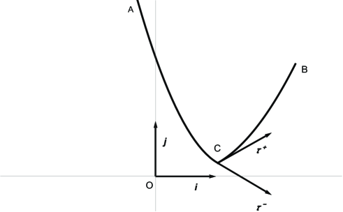
Figure 1: A heavy ring $C$ can freely slide on a heavy curve of total length $\ell$ and fixed at the end points $A$ and $B$ in the vertical plane $(O,\,\boldsymbol{i},\,\boldsymbol{j})$. One needs to find the position of $C$ as well as the corresponding equilibrium curve.

This equation is supplemented by two jump conditions at point $C$ coming from (1) :

$$-n(C)\left[\boldsymbol{\tau}\right]+mg\,{\boldsymbol{j}}=\boldsymbol{0}$$

Since $n(c)\neq 0$, we finally obtain :

$$\left\{\begin{array}[]{l}\displaystyle\left[\boldsymbol{\tau}^{T}\right]{\boldsymbol{i}}=0\\ \\ \displaystyle n(C)\left[\boldsymbol{\tau}^{T}\right]{\boldsymbol{j}}-mg=0\end{array}\right.$$ (1.10)

Consequently, the angles between tangent vectors to the curve and the horizontal axe are opposite. The second condition determines the Lagrange multiplier $\it\Lambda$. The conditions (1.10) can be seen as Rankine–Hugoniot conditions which complement the governing equations and define boundary conditions for the ‘broken extremal’ (Figure 1).

Such a variational technique can be generalized to the case of continuum mechanics where the variation of Hamilton’s action should naturally be considered in the four-dimensional physical space-time [34, 35, 36].

The remainder of this paper is structured as follows. In Section 2 the variation of Hamilton’s action with a generic Lagrangian depending on the thermodynamic variables and their space-time derivatives is found. The corresponding Euler–Lagrange equations are specified for the capillary fluids and for the bubbly fluids in Section 3. The Rankine–Hugoniot conditions for both models are derived in Section 4. Technical details are given in Appendix.

2 The Hamilton action

Consider the Hamilton action :

$$a=\int_{\mathcal{W}}L\,d\boldsymbol{z}$$

where $\mathcal{W}$ is a 4-D domain in space–time. The Lagrangian is in the form :

$$L=\mathcal{L}\left(\boldsymbol{J},\frac{\partial\boldsymbol{J}}{\partial\boldsymbol{z}},\eta,\boldsymbol{z}\right)$$

with $\boldsymbol{z}=\left(\begin{array}[]{c}t\\ \boldsymbol{x}\end{array}\right)\equiv\left\{z^{i}\right\}$, where $z^{0}=t$ is the time and $\boldsymbol{x}\equiv\left\{x^{i}\right\}$, $i=1,2,3$ are the Euler space-variables. We write $\boldsymbol{J}=\left(\begin{array}[]{c}\rho\\ \rho\boldsymbol{u}\end{array}\right)$, where $\rho$ is the fluid density, $\eta$ is the specific entropy (the entropy per unit mass) and $\boldsymbol{u}$ is the fluid velocity. The 4-D vector $\boldsymbol{J}$ verifies the mass conservation :

$$\text{Div}\boldsymbol{J}\equiv\dfrac{\partial\rho}{\partial t}+\text{div}(\rho\boldsymbol{u})=0$$ (2.11)

where div and Div are the divergence operators in the 3-D physical space and in 4-D physical space-time, respectively. For conservative motion, due to (2.11), the equation for the entropy $\eta$ takes the form :

$$\text{Div}\left(\eta\,\boldsymbol{J}\right)\equiv\dfrac{\partial\rho\eta}{\partial t}+\text{div}(\rho\eta\,\boldsymbol{u})=0$$ (2.12)

To calculate the variation of Hamilton’s action, we consider a one-parameter family of virtual motions :

$${\boldsymbol{z}}=\boldsymbol{\Phi}(\boldsymbol{Z},\varepsilon)\quad\text{with}\quad\boldsymbol{\Phi}(\boldsymbol{Z},0)=\boldsymbol{\varphi}(\boldsymbol{Z})$$ (2.13)

where $\boldsymbol{z}=\boldsymbol{\varphi}(\boldsymbol{Z})$ represents the real motion and $\boldsymbol{\Phi}$ is a regular function in the 4-D reference-space $\mathcal{W}_{0}$ of variables $\boldsymbol{Z}\equiv\left(Z^{i}\right),(i=0,1,2,3)$ : $Z^{0}=\lambda$ is a scalar field (which is not necessarily the time), $\boldsymbol{X}\equiv\left(X^{i}\right),(i=1,2,3)$ are the Lagrange variables. The scalar $\varepsilon$ is a real parameter defined in the vicinity of zero.
We define the virtual displacements $\tilde{\delta}{\boldsymbol{z}}(\boldsymbol{Z})$ and the Lagrangian variations $\tilde{\delta}\boldsymbol{J(Z)}$ by the formulas :

$$\tilde{\delta}{\boldsymbol{z}}({\boldsymbol{Z}})=\left.\frac{\partial\boldsymbol{\Phi}({\boldsymbol{Z}},\varepsilon)}{\partial\varepsilon}\right|_{\varepsilon=0}$$

$$\tilde{\delta}\boldsymbol{J(Z)}=\left.\frac{\partial\boldsymbol{J(Z},\varepsilon\boldsymbol{)}}{\partial\varepsilon}\right|_{\varepsilon=0}$$

Due to the fact that $\boldsymbol{Z}=\boldsymbol{\varphi}^{-1}\boldsymbol{(z)}$, we can also consider the variations as functions of Eulerian variables. Further, we use the notation $\boldsymbol{\zeta}(\boldsymbol{z})=\tilde{\delta}\boldsymbol{z}\left(\boldsymbol{\varphi}^{-1}\boldsymbol{(}z)\right)$ and we write $\delta\boldsymbol{J(z)}$ and other quantities without tilde in Eulerian variables: $\delta\boldsymbol{J(z)}=\tilde{\delta}\boldsymbol{J}\left(\boldsymbol{\varphi}^{-1}\boldsymbol{(}z)\right)$. The Hamilton principle assumes $\boldsymbol{\zeta}(\boldsymbol{z})=0$ on the external boundary $\partial\mathcal{W}$ of $\mathcal{W}$.
Let $\boldsymbol{\zeta}^{T}=\left(\tau,\boldsymbol{\xi}^{T}\right)$, where ${\tau}$ is the scalar part of 4-vector $\boldsymbol{\zeta}$ associated with time $t$ and 3-vector $\boldsymbol{\xi}$ is the part of 4-vector $\boldsymbol{\zeta}$ associated with space-variable $\boldsymbol{x}$.
In calculations we use the relation :

$$\delta\boldsymbol{J}=\left(\frac{\partial\boldsymbol{\zeta}}{\partial\boldsymbol{z}}-\left(\text{Div}\,\boldsymbol{\zeta}\right)I_{4}\right)\boldsymbol{J}$$ (2.14)

(see Appendix A for the proof).
Due to (2.12), the variation of the specific entropy is zero [37] :

$$\delta\eta=0$$

It is the reason, we don’t always indicate $\eta$ in expression of the Lagrangian, even if the entropy is explicitly presented in the governing equations.

The variation of Hamilton’s action is calculated for the family of virtual motions (2.13) :

$$\delta a=\left.\frac{da}{d\varepsilon}\right|_{\varepsilon=0}=\int_{\mathcal{W}}\left(\delta L+L\,\text{Div}\,\boldsymbol{\zeta}\right)d\boldsymbol{z}$$ (2.15)

and

$$\delta L=\frac{\partial L}{\partial\boldsymbol{J}}\ \delta\boldsymbol{J}+\text{Tr}\left(\frac{\partial L}{\partial\left(\dfrac{\partial\boldsymbol{J}}{\partial\boldsymbol{z}}\right)}\,\delta\left(\frac{\partial\boldsymbol{J}}{\partial\boldsymbol{z}}\right)\right)+\frac{\partial L}{\partial\boldsymbol{z}}\ \boldsymbol{\zeta}$$

To obtain (2.15) we use Jacobi’s identity for the generalized 4-D deformation gradient $\mathcal{B}$ :

$$\delta\,\text{det}\,\mathcal{B}=\text{det}\,\mathcal{B}\ \text{Div}\,\boldsymbol{\zeta}\quad\text{with}\quad\mathcal{B}=\frac{\partial\boldsymbol{z}}{\partial\boldsymbol{Z}}$$

To simplify the notation we write :

$$\mathcal{C}=\frac{\partial\boldsymbol{J}}{\partial\boldsymbol{z}},\,\ \mathcal{A}^{T}=\frac{\partial L}{\partial\left(\dfrac{\partial\boldsymbol{J}}{\partial\boldsymbol{z}}\right)}=\left(\nabla_{\mathcal{C}}L\right)^{T}\,\ \text{and}\,\,\ \text{Tr}\left(\mathcal{A}^{T}\,\delta\mathcal{C}\right)=\nabla_{\mathcal{C}}L:\delta\mathcal{C}$$

One also has :

$$\delta\mathcal{C}=\delta\left(\frac{\partial\boldsymbol{J}}{\partial\boldsymbol{z}}\right)=\delta\,\left(\frac{\partial\boldsymbol{J}}{\partial\boldsymbol{Z}}\ \frac{\partial\boldsymbol{Z}}{\partial\boldsymbol{z}}\right)=\frac{\partial\delta\boldsymbol{J}}{\partial\boldsymbol{z}}-\frac{\partial\boldsymbol{J}}{\partial\boldsymbol{z}}\frac{\partial\boldsymbol{\zeta}}{\partial\boldsymbol{z}}$$

For the sake of simplicity, in the following the measure of integration will not be indicated. Then, we get from (2.14) and (2.15) :

$$\delta a = \int_{\mathcal{W}}\frac{\partial L}{\partial\boldsymbol{J}}\left(\frac{\partial\boldsymbol{\zeta}}{\partial\boldsymbol{z}}-\left(\text{Div}\ \boldsymbol{\zeta}\right)\boldsymbol{I}_{4}\right)\boldsymbol{J}+\text{Tr}\left(\mathcal{A}^{T}\left(\frac{\partial\delta\boldsymbol{J}}{\partial\boldsymbol{z}}-\frac{\partial\boldsymbol{J}}{\partial\boldsymbol{z}}\frac{\partial\boldsymbol{\zeta}}{\partial\boldsymbol{z}}\right)\right)+\frac{\partial L}{\partial\boldsymbol{z}}\ \boldsymbol{\zeta}+L\,\text{Div}\ \boldsymbol{\zeta}$$

One has :

$$\delta a=\int_{\mathcal{W}}\text{Tr}\left(\left(\boldsymbol{J}\frac{\partial L}{\partial\boldsymbol{J}}-\mathcal{A}^{T}\frac{\partial\boldsymbol{J}}{\partial\boldsymbol{z}}\right)\frac{\partial{\boldsymbol{\zeta}}}{\partial\boldsymbol{z}}\right)+\left(L-\frac{\partial L}{\partial\boldsymbol{J}}\ \boldsymbol{J}\right)\text{Div}\ {\boldsymbol{\zeta}}+\text{Tr}\left(\mathcal{A}^{T}\frac{\partial\delta\boldsymbol{J}}{\partial\boldsymbol{z}}\right)+\frac{\partial L}{\partial\boldsymbol{z}}\ {{\boldsymbol{\zeta}}}$$

$$=\int_{\mathcal{W}}\text{Tr}\left(\left(\boldsymbol{J}\frac{\partial L}{\partial\boldsymbol{J}}-\mathcal{A}^{T}\frac{\partial\boldsymbol{J}}{\partial\boldsymbol{z}}\right)\frac{{\boldsymbol{\partial\zeta}}}{\partial\boldsymbol{z}}\right)+\left(L-\frac{\partial L}{\partial\boldsymbol{J}}\ \boldsymbol{J}\right)\text{Div}\ {\boldsymbol{\zeta}}+\text{Div}\left(\mathcal{A}^{T}\delta\boldsymbol{J}\right)-\text{Div}\left(\mathcal{A}^{T}\right)\delta\boldsymbol{J}+\frac{\partial L}{\partial\boldsymbol{z}}\ {\boldsymbol{\zeta}}$$

and finally :

$$\delta a = \int_{\mathcal{W}}\text{Tr}\left(\left(\boldsymbol{J}\frac{\partial L}{\partial\boldsymbol{J}}-\mathcal{A}^{T}\frac{\partial\boldsymbol{J}}{\partial\boldsymbol{z}}\right)\frac{\partial\boldsymbol{\zeta}}{\partial\boldsymbol{z}}\right)\boldsymbol{+}\left(L-\frac{\partial L}{\partial\boldsymbol{J}}\ \boldsymbol{J}\right)\text{Div}\ \boldsymbol{\zeta}+\text{Div}\left(\mathcal{A}^{T}\delta\boldsymbol{J}\right)$$

$$- \int_{\mathcal{W}}\text{Div}\left(\mathcal{A}^{T}\right)\left(\frac{\partial{\boldsymbol{\zeta}}}{\partial\boldsymbol{z}}-\left(\text{Div}\ {{\boldsymbol{\zeta}}}\right)\boldsymbol{I}_{4}\right)\boldsymbol{J}+\frac{\partial L}{\partial\boldsymbol{z}}\,{\boldsymbol{\zeta}}$$

$$= \int_{\mathcal{W}}\text{Tr}\left(\left(\boldsymbol{J}\frac{\partial L}{\partial\boldsymbol{J}}-\mathcal{A}^{T}\frac{\partial\boldsymbol{J}}{\partial\boldsymbol{z}}-\boldsymbol{J}\,\text{Div}\left(\mathcal{A}^{T}\right)\right)\frac{\partial{\boldsymbol{\zeta}}}{\partial\boldsymbol{z}}\right)$$

$$+ \int_{\mathcal{W}}\left(L-\frac{\partial L}{\partial\boldsymbol{J}}\ \boldsymbol{J}+\left(\text{Div}\mathcal{A}^{T}\right)\boldsymbol{J}\right)\text{Div}\ {{\boldsymbol{\zeta}}}+\text{Div}\left(\mathcal{A}^{T}\delta\boldsymbol{J}\right)+\frac{\partial L}{\partial\boldsymbol{z}}\ \boldsymbol{\zeta}$$

$$= \int_{\mathcal{W}}\text{Div}\left(\left(\boldsymbol{J}\frac{\partial L}{\partial\boldsymbol{J}}-\mathcal{A}^{T}\frac{\partial\boldsymbol{J}}{\partial\boldsymbol{z}}-\boldsymbol{J}\ \text{Div}\left(\mathcal{A}^{T}\right)\right){{\boldsymbol{\zeta}}}+\mathcal{A}^{T}\delta\boldsymbol{J}\right)$$

$$- \int_{\mathcal{W}}\text{Div}\left(\boldsymbol{J}\frac{\partial L}{\partial\boldsymbol{J}}-\mathcal{A}^{T}\frac{\partial\boldsymbol{J}}{\partial\boldsymbol{z}}-\boldsymbol{J}\,\text{Div}\left(\mathcal{A}^{T}\right)\right)\boldsymbol{\zeta}$$

$$+ \int_{\mathcal{W}}\text{Div}\left(\left(L-\frac{\partial L}{\partial\boldsymbol{J}}\boldsymbol{J}+\left(\text{Div}\mathcal{A}^{T}\right)\boldsymbol{J}\right){{\boldsymbol{\zeta}}}\right)$$

$$- \int_{\mathcal{W}}\text{Grad}\left(L-\frac{\partial L}{\partial\boldsymbol{J}}\boldsymbol{J}+\left(\text{Div}\mathcal{A}^{T}\right)\boldsymbol{J}\right)^{T}\boldsymbol{\zeta}+\frac{\partial L}{\partial\boldsymbol{z}}\ {{\boldsymbol{\zeta}}}$$

Let us denote :

$$\boldsymbol{K}^{T}=\frac{\delta L}{\delta\boldsymbol{J}}\equiv\frac{\partial L}{\partial\boldsymbol{J}}-\text{Div}\left(\mathcal{A}^{T}\right)$$

then :

$$\delta a = \int_{\mathcal{W}}\left\{\frac{\partial L}{\partial\boldsymbol{z}}-\text{Div}\left(\boldsymbol{J}\boldsymbol{K}^{T}-\mathcal{A}^{T}\frac{\partial\boldsymbol{J}}{\partial\boldsymbol{z}}+p\,\boldsymbol{I}_{4}\right)\right\}\ {{\boldsymbol{\zeta}}}$$

$$+ \int_{\partial\mathcal{W}}{\boldsymbol{N}^{T}}\left(\boldsymbol{J}\ \boldsymbol{K}^{T}-\mathcal{A}^{T}\frac{\partial\boldsymbol{J}}{\partial\boldsymbol{z}}+p\,\boldsymbol{I}_{4}\right){{\boldsymbol{\zeta}}}+{\boldsymbol{N}^{T}}\mathcal{A}^{T}\delta\boldsymbol{J}$$

where

$$p=L-\boldsymbol{K}^{T}\boldsymbol{J}$$ (2.16)

and $\boldsymbol{N}^{T}$ is a 4-D co-vector canceling the tangent vectors to $\partial\mathcal{W}$.

Due to the fact, the virtual displacement can be considered as null in the vicinity of the boundary $\partial\mathcal{W}$, the Hamilton principle simply writes :

$$\delta a = \int_{\mathcal{W}}\left\{\frac{\partial L}{\partial\boldsymbol{z}}-\text{Div}\left(\boldsymbol{J}\boldsymbol{K}^{T}-\mathcal{A}^{T}\frac{\partial\boldsymbol{J}}{\partial\boldsymbol{z}}+p\,\boldsymbol{I}_{4}\right)\right\}\ {{\boldsymbol{\zeta}}}=0$$

and we get the equations of motions in a conservative form [38] :

$$\text{ Div}\left(\boldsymbol{J}\,\boldsymbol{K}^{T}-\mathcal{A}^{T}\frac{\partial\boldsymbol{J}}{\partial\boldsymbol{z}}+p\,\boldsymbol{I}_{4}\right)=\frac{\partial L}{\partial\boldsymbol{z}}$$ (2.17)

where term $\partial L/\partial\boldsymbol{z}$ is associated with the external body forces.

Let the motion be discontinuous on a 3-D surface $\it\it\Sigma$ with normal $\boldsymbol{N}$ (see Figure 2). The virtual displacement can be considered as null in the vicinity of the boundary $\partial\mathcal{W}$, and equations of motions (2.17) being satisfied, the variation of the Hamilton action is reduced to :

$$\delta a=\int_{\it\it\Sigma}\left[{\boldsymbol{N}^{T}}\left(\boldsymbol{J}\boldsymbol{K}^{T}-A^{T}\frac{\partial\boldsymbol{J}}{\partial\boldsymbol{z}}+p\,\boldsymbol{I}_{4}\right){{\boldsymbol{\zeta}}}+{\boldsymbol{N}^{T}}A^{T}\delta\boldsymbol{J}\right]$$ (2.18)

where the brackets $\left[\,\,\right]$ mean the jumps of discontinuous quantities across $\it\it\Sigma$.

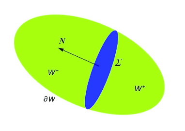
Figure 2: The shock surface $\it\it\Sigma$ in $\mathcal{W}$: The shock surface $\it\it\Sigma$ divides the space-time domain $\mathcal{W}$ into two space-time domains $\mathcal{W}^{-}$ and $\mathcal{W}^{+}$ behind and ahead of the shock in which the solution is continuous but across the shock.

In the next section, we explicit the governing equation (2.17) for two cases : second gradient fluids and bubbly fluids. Then, we present the surface integral (2.18) for these two specific cases.

3 Particular cases

3.1 Capillary fluids

Without body forces, the Lagrangian is of the form :

$$L=\frac{1}{2}\,\rho\,\left|\boldsymbol{u}\right|^{2}-\rho\,\alpha\left(\rho,\frac{\partial\rho}{\partial\boldsymbol{x}},\eta\right)\equiv\frac{1}{2\,\rho}\,\left|\boldsymbol{j}\right|^{2}-\rho\,\alpha\left(\rho,\frac{\partial\rho}{\partial\boldsymbol{x}},\eta\right)$$

Then

$$\frac{\partial\boldsymbol{J}}{\partial\boldsymbol{z}}=\left(\begin{array}[]{ll}\;\dfrac{\partial\rho}{\partial t}&\;\dfrac{\partial\rho}{\partial\boldsymbol{x}}\\ \begin{array}[]{l}\\ \dfrac{\partial\boldsymbol{j}}{\partial t}\end{array}&\begin{array}[]{l}\\ \dfrac{\partial\boldsymbol{j}}{\partial\boldsymbol{x}}\end{array}\end{array}\right),\quad\frac{\partial L}{\partial\boldsymbol{J}}=\left(-\frac{1}{2}\,\left|\boldsymbol{u}\right|^{2}-\alpha-\rho\,\dfrac{\partial\alpha}{\partial\rho},\ \boldsymbol{u}^{T}\right)$$ (3.19)

We deduce :

$$\mathcal{A}^{T}=\frac{\partial L}{\partial\left(\dfrac{\partial\boldsymbol{J}}{\partial\boldsymbol{z}}\right)}=\left(\begin{array}[]{ll}\quad\quad\quad 0&\;\boldsymbol{0}_{3}^{T}\\ \begin{array}[]{l}\\ -\rho\,\dfrac{\partial\alpha}{\partial\left(\dfrac{\partial\rho}{\partial\boldsymbol{x}}\right)}\end{array}&\begin{array}[]{l}\\ O_{3}\end{array}\end{array}\right)$$ (3.20)

and get :

$$\text{Div}\,(\mathcal{A}^{T})=-\left(\text{div}\left\{\rho\,\dfrac{\partial\alpha}{\partial\left(\dfrac{\partial\rho}{\partial\boldsymbol{x}}\right)}\right\},\;\boldsymbol{0}^{T}_{3}\right)$$

$$\boldsymbol{K}^{T}=\frac{\partial L}{\partial\boldsymbol{J}}-\text{Div}\,(\mathcal{A}^{T})=\left(-\frac{1}{2}\left|\boldsymbol{u}\right|^{2}-\alpha-\rho\,\dfrac{\partial\alpha}{\partial\rho}+\text{div}\left\{\rho\,\dfrac{\partial\alpha}{\partial\left(\dfrac{\partial\rho}{\partial\boldsymbol{x}}\right)}\right\},\ \boldsymbol{u}^{T}\right)$$ (3.21)

The pressure $p$ deduced from (2.16) is defined as :

$$p\equiv\rho^{2}\,\dfrac{\partial\alpha}{\partial\rho}-\rho\ \text{div}\left(\rho\,\dfrac{\partial\alpha}{\partial\left(\dfrac{\partial\rho}{\partial\boldsymbol{x}}\right)}\right)$$

Nevertheless, $p$ is not only a function of density as in the case of barotropic fluids: it depends also on the density gradient. Additively :

$$\mathcal{A}^{T}\frac{\partial\boldsymbol{J}}{\partial\boldsymbol{z}}=\left(\begin{array}[]{ll}\qquad\quad 0,&\qquad\quad\boldsymbol{0}_{3}^{T}\\ \begin{array}[]{l}\\ -\rho\,\dfrac{\partial\alpha}{\partial\left(\dfrac{\partial\rho}{\partial\boldsymbol{x}}\right)}\dfrac{\partial\rho}{\partial t},\end{array}&\begin{array}[]{l}\\ -\rho\,\dfrac{\partial\alpha}{\partial\left(\dfrac{\partial\rho}{\partial\boldsymbol{x}}\right)}\dfrac{\partial\rho}{\partial\boldsymbol{x}}\end{array}\end{array}\right)$$

$$\boldsymbol{J}\boldsymbol{K}^{T}=\left(\begin{array}[]{ll}\quad-\dfrac{1}{2}\rho\,\left|\boldsymbol{u}\right|^{2}-\rho\,\alpha-p,&\;\ \rho\,\boldsymbol{u}^{T}\\ \begin{array}[]{l}\\ \left(-\dfrac{1}{2}\rho\,\left|\boldsymbol{u}\right|^{2}-\rho\,\alpha-p\right)\boldsymbol{u},\end{array}&\begin{array}[]{l}\\ \rho\,\boldsymbol{u}\boldsymbol{u}^{T}\end{array}\end{array}\right)$$

Equation (2.17) writes :

$${\text{Div}}\left(\begin{array}[]{ll}\qquad\qquad e,&\qquad\qquad-\rho\,\boldsymbol{u}^{T}\\ \begin{array}[]{l}\\ \left(e+p\right)\boldsymbol{u}-\rho\,\dfrac{\partial\rho}{\partial t}\dfrac{\partial\alpha}{\partial\left(\dfrac{\partial\rho}{\partial\boldsymbol{x}}\right)},\end{array}&\begin{array}[]{l}\\ -\rho\,\boldsymbol{u}\boldsymbol{u}^{T}-\rho\,\dfrac{\partial\alpha}{\partial\left(\dfrac{\partial\rho}{\partial\boldsymbol{x}}\right)}\dfrac{\partial\rho}{\partial\boldsymbol{x}}-p\,\boldsymbol{I}_{3}\end{array}\end{array}\right)=\boldsymbol{0}^{T}_{4}$$ (3.22)

where we denote by

$$e=\rho\,\left(\frac{1}{2}\,\left|\boldsymbol{u}\right|^{2}+\alpha\right)$$

the total energy per unit volume of the fluid; the first component of Eq. (3.22) yields the equation of energy :

$$\frac{\partial e}{\partial t}+{\text{d}iv}\left(\left(e+p\right)\boldsymbol{u}-\rho\,\dfrac{\partial\rho}{\partial t}\dfrac{\partial\alpha}{\partial\left(\dfrac{\partial\rho}{\partial\boldsymbol{x}}\right)}\right)=0$$ (3.23)

The additive term $\rho\,\dfrac{\partial\rho}{\partial t}\dfrac{\partial\alpha}{\partial\left(\dfrac{\partial\rho}{\partial\boldsymbol{x}}\right)}$ is a flux of energy corresponding to the interstitial working [22].
The three other components of Eq. (3.22) yield the equations of motion :

$$\frac{\partial\rho\,\boldsymbol{u}^{T}}{\partial t}+\text{div}\left(\rho\,\boldsymbol{u}\otimes\boldsymbol{u}+p\,\boldsymbol{I}+\rho\,\dfrac{\partial\alpha}{\partial\left(\dfrac{\partial\rho}{\partial\boldsymbol{x}}\right)}\dfrac{\partial\rho}{\partial\boldsymbol{x}}\right)=\boldsymbol{0}^{T}$$ (3.24)

Equations (3.23) and (3.24) represent the development of (2.17) for capillary fluids.

3.2 Bubbly fluids

Without body forces, the Lagrangian is of the form :

$$L=\frac{1}{2}\,\rho\,\left|\boldsymbol{u}\right|^{2}-\rho\,w\left(\rho,\dot{\rho},\eta\right)\equiv\frac{1}{2\,\rho}\,\left|\boldsymbol{j}\right|^{2}-\rho\,w\left(\rho,\dot{\rho},\eta\right)$$

where

$$\overset{\centerdot}{\rho}=\dfrac{d\rho}{dt}=\dfrac{\;\partial\rho}{\partial t}+\frac{\partial\rho}{\partial\boldsymbol{x}}\,{\boldsymbol{u}}\equiv\dfrac{\partial\rho}{\partial t}+\frac{1}{\rho}\,\frac{\partial\rho}{\partial\boldsymbol{x}}\,{\boldsymbol{j}}$$

Such a Lagrangian appears in the study of wave propagation for shallow water flows with dispersion and bubbly flows (a complete discussion of these models is given in [39]). Then (3.19) can be explicitly written as :

$$\frac{\partial L}{\partial\boldsymbol{J}}=\left(-\frac{1}{2}\,\left|\boldsymbol{u}\right|^{2}-w-\rho\,\dfrac{\partial w}{\partial\rho}+\dfrac{\partial w}{\partial\overset{\centerdot}{\rho}}\frac{\partial\rho}{\partial\boldsymbol{x}}\,\boldsymbol{u},\,\ \boldsymbol{u}^{T}-\dfrac{\partial w}{\partial\overset{\centerdot}{\rho}}\frac{\partial\rho}{\partial\boldsymbol{x}}\right)$$

We deduce :

$$\mathcal{A}^{T}=\frac{\partial L}{\partial\left(\dfrac{\partial\boldsymbol{J}}{\partial\boldsymbol{z}}\right)}=\left(\begin{array}[]{ll}\ \;-\rho\,\dfrac{\partial w}{\partial\overset{\centerdot}{\rho}}&\;\boldsymbol{0}_{3}^{T}\\ \begin{array}[]{l}\\ -\rho\,\dfrac{\partial w}{\partial\overset{\centerdot}{\rho}}\,\boldsymbol{u}\end{array}&\begin{array}[]{l}\\ O_{3}\end{array}\end{array}\right)$$ (3.25)

Due to (2.11) we obtain :

$$\text{Div}\,(\mathcal{A}^{T})=\left(-\dfrac{\partial}{\partial t}\left(\rho\,\dfrac{\partial w}{\partial\overset{\centerdot}{\rho}}\right)-\text{div}\left(\rho\,\dfrac{\partial w}{\partial\overset{\centerdot}{\rho}}\boldsymbol{u}\right),\;\boldsymbol{0}^{T}_{3}\right)\equiv\left(-\rho\,\dfrac{d}{dt}\left(\dfrac{\partial w}{\partial\overset{\centerdot}{\rho}}\right),\;\boldsymbol{0}^{T}_{3}\right)$$

$$\boldsymbol{K}^{T} = \frac{\partial L}{\partial\boldsymbol{J}}-\text{Div}\,(\mathcal{A}^{T})$$

$$= \left(-\frac{1}{2}\,\left|\boldsymbol{u}\right|^{2}-w-\rho\,\dfrac{\partial w}{\partial\rho}+\dfrac{\partial w}{\partial\overset{\centerdot}{\rho}}\frac{\partial\rho}{\partial\boldsymbol{x}}\,\boldsymbol{u}+\rho\,\dfrac{d}{dt}\left(\dfrac{\partial w}{\partial\overset{\centerdot}{\rho}}\right),\ \ \boldsymbol{u}^{T}-\dfrac{\partial w}{\partial\overset{\centerdot}{\rho}}\frac{\partial\rho}{\partial\boldsymbol{x}}\right)$$

The pressure $p$ obtained from (2.16) is defined as :

$$p=\rho^{2}\left(\dfrac{\partial w}{\partial\rho}-\dfrac{d}{dt}\left(\dfrac{\partial w}{\partial\overset{\centerdot}{\rho}}\right)\right)$$

Nevertheless pressure $p$ depends also on the material derivatives of the density. Additively,

$$\mathcal{A}^{T}\frac{\partial\boldsymbol{J}}{\partial\boldsymbol{z}}=\left(\begin{array}[]{ll}\;-\rho\,\dfrac{\partial w}{\partial\overset{\centerdot}{\rho}}\dfrac{\partial\rho}{\partial t},&\;-\rho\,\dfrac{\partial w}{\partial\overset{\centerdot}{\rho}}\dfrac{\partial\rho}{\partial\boldsymbol{x}}\\ \begin{array}[]{l}\\ -\rho\,\dfrac{\partial w}{\partial\overset{\centerdot}{\rho}}\dfrac{\partial\rho}{\partial t}\boldsymbol{u},\end{array}&\begin{array}[]{l}\\ -\rho\,\dfrac{\partial w}{\partial\overset{\centerdot}{\rho}}\boldsymbol{u}\dfrac{\partial\rho}{\partial\boldsymbol{x}}\end{array}\end{array}\right)$$

$$\boldsymbol{J}\boldsymbol{K}^{T}=\left(\begin{array}[]{ll}-\dfrac{1}{2}\rho\,\left|\boldsymbol{u}\right|^{2}-\rho\,w-p+\rho\,\dfrac{\partial w}{\partial\overset{\centerdot}{\rho}}\dfrac{\partial\rho}{\partial\boldsymbol{x}}\boldsymbol{u},&\;\ \rho\,\boldsymbol{u}^{T}-\rho\,\dfrac{\partial w}{\partial\overset{\centerdot}{\rho}}\dfrac{\partial\rho}{\partial\boldsymbol{x}}\\ \begin{array}[]{l}\\ \left(-\dfrac{1}{2}\rho\,\left|\boldsymbol{u}\right|^{2}-\rho\,w-p+\rho\,\dfrac{\partial w}{\partial\overset{\centerdot}{\rho}}\dfrac{\partial\rho}{\partial\boldsymbol{x}}\boldsymbol{u}\right)\boldsymbol{u},\end{array}&\begin{array}[]{l}\\ \rho\,\boldsymbol{u}\boldsymbol{u}^{T}-\rho\,\dfrac{\partial w}{\partial\overset{\centerdot}{\rho}}\boldsymbol{u}\dfrac{\partial\rho}{\partial\boldsymbol{x}}\end{array}\end{array}\right)$$

Equation (2.17) writes :

$${\text{Div}}\left(\begin{array}[]{ll}\quad\dfrac{1}{2}\rho\,\left|\boldsymbol{u}\right|^{2}+\rho\,w-\rho\,\dfrac{\partial w}{\partial\overset{\centerdot}{\rho}}\overset{\centerdot}{\rho},&\;\ -\rho\,\boldsymbol{u}^{T}\\ \begin{array}[]{l}\\ \left(\dfrac{1}{2}\rho\,\left|\boldsymbol{u}\right|^{2}+\rho\,w-\rho\,\dfrac{\partial w}{\partial\overset{\centerdot}{\rho}}\overset{\centerdot}{\rho}+p\right)\boldsymbol{u},\end{array}&\begin{array}[]{l}\\ -\rho\,\boldsymbol{u}\boldsymbol{u}^{T}-p\,\boldsymbol{I}_{3}\end{array}\end{array}\right)=\boldsymbol{0}^{T}_{4}$$ (3.26)

We denote by

$$e=\rho\,\left(\frac{1}{2}\,\left|\boldsymbol{u}\right|^{2}+w-\overset{\centerdot}{\rho}\,\frac{\partial w}{\partial\overset{\centerdot}{\rho}}\right)$$

the total energy per unit volume of the fluid; the first component of Eq. (3.26) yields the equation of energy :

$$\frac{\partial e}{\partial t}+{\text{d}iv}\left(\left(e+p\right)\boldsymbol{u}\right)=0$$ (3.27)

The three other components of Eq. (3.26) yield the equations of motion :

$$\frac{\partial\rho\boldsymbol{u}^{T}}{\partial t}+\text{div}(\rho\boldsymbol{u}\otimes\boldsymbol{u}+p\,I)={\bf 0}^{T}$$ (3.28)

Equations (3.27) and (3.28) represent the development of (2.17) for bubbly fluids.

4 Rankine–Hugoniot conditions

We represent $\it\it\Sigma$ in the form ${\it\Sigma}=[t_{0},t_{1}]\times S_{t}$ where $S_{t}$ is a time dependent surface. Then, $\boldsymbol{N}^{T}=(-D_{n},\boldsymbol{n}^{T})$, where $D_{n}$ denotes the normal surface velocity of $S_{t}$ and $\boldsymbol{n}$ is the unit normal vector to $S_{t}$. The mass conservation law (2.11) yields the relation :

$$\left[\boldsymbol{N}^{T}\boldsymbol{J}\right]=\left[\rho\left(\boldsymbol{n}^{T}\boldsymbol{u}-D_{n}\right)\right]=[\rho\,v]=0\qquad\text{with}\,\ v=\boldsymbol{n}^{T}\boldsymbol{u}-D_{n}$$

As seen in Appendix 2, in the two particular cases, the term $\boldsymbol{N}^{T}\mathcal{A}^{T}\delta\boldsymbol{J}$ can be written as :

$$\boldsymbol{N}^{T}\mathcal{A}^{T}\delta\boldsymbol{J}=b\,\left(\text{div}\,\boldsymbol{\xi}-\frac{\partial\tau}{\partial\boldsymbol{x}}\boldsymbol{u}\right)$$

where $b$ is the scalar which is given in explicit form for capillary fluids by (B.37) and for bubbly fluids by (B.38) .

We study the case when $\it\it\Sigma$ is a shock surface and consequently $\rho\,v=\boldsymbol{N}^{T}\boldsymbol{J}\neq 0$.

Equation (2.17) being verified, we obtain for all vector field $\boldsymbol{\zeta}$ the variation of $\delta a$ in the form (2.18). The surface integral (2.18) will be presented in separable form in terms of virtual displacements and their normal derivatives along the 3-D manifold $\it\Sigma$ [40, 41].
Using Lemmas from Appendix C, we obtain :

$$\boldsymbol{N}^{T}\mathcal{A}^{T}\delta\boldsymbol{J} = b\,\left(\text{div}\,\boldsymbol{\xi}-\frac{\partial\tau}{\partial\boldsymbol{x}}\boldsymbol{u}\right)=b\,\text{div}(\boldsymbol{\xi}-\tau\boldsymbol{u})+\tau\,b\,\text{div}(\boldsymbol{u})$$

$$= -\boldsymbol{\it\Theta}^{T}\boldsymbol{\zeta}-b\,\boldsymbol{n}^{T}\boldsymbol{u}\,\frac{d\tau}{dn}+b\,\frac{d{\xi}_{n}}{dn}+\boldsymbol{n}^{T}\,{\rm rot}\,\left(\boldsymbol{n}\times b\,\left(\boldsymbol{\xi}-\tau\boldsymbol{u}\right)\right),$$

with

$$\boldsymbol{\it\Theta}=\left(\begin{array}[]{c}-b\,H\boldsymbol{n}^{T}\boldsymbol{u}-\text{div}_{tg}\,(b\,\boldsymbol{u})\\ \\ b\,H\boldsymbol{n}+\nabla_{tg}b+\displaystyle b\frac{\partial\boldsymbol{n}}{\partial\boldsymbol{x}}\boldsymbol{n}\end{array}\right).$$ (4.29)

Here we use the notations $\displaystyle\nabla_{tg}^{T}b=\dfrac{\partial b}{\partial\boldsymbol{x}}\left(\boldsymbol{I}-\boldsymbol{n}\boldsymbol{n}^{T}\right)$ and $\displaystyle\text{div}_{tg}(b\mathbf{u})=\text{div}\,\left(b\,\boldsymbol{u}\right)-\boldsymbol{n}^{T}\,\frac{\partial b\,\boldsymbol{u}}{\partial\boldsymbol{x}}\,\boldsymbol{n}$, where index ‘tg’ means the tangential gradient and tangential divergence operators to $S_{t}$. Also, $H=-\text{div}(\boldsymbol{n})$ is the sum of principal curvatures of $S_{t}$. From (2.18), one obtains :

$$\delta a = \int_{\it\Sigma}\left[\left\{\boldsymbol{N}^{T}\left(\boldsymbol{J}\boldsymbol{K}^{T}-\mathcal{A}^{T}\frac{\partial\boldsymbol{J}}{\partial\boldsymbol{z}}+p\,\boldsymbol{I}_{4}\right)-\boldsymbol{\it\Theta}^{T}\right\}\boldsymbol{\zeta}\right]$$

$$- \int_{\it\Sigma}\left[b\,\boldsymbol{n}^{T}\boldsymbol{u}\,\frac{d\tau}{dn}-b\,\frac{d{\xi}_{n}}{dn}\right]+\int_{t_{0}}^{t_{1}}\int_{C_{t}}\left[b\,\left\{\boldsymbol{n}\times\left(\boldsymbol{\xi}-\tau\boldsymbol{u}\right)\right\}^{T}\boldsymbol{t}\right]$$

Here $C_{t}$ denotes the boundary of $S_{t}$ ($\it\Sigma=[t_{0},t_{1}]\times S_{t}$), and $\boldsymbol{t}$ is the oriented unit tangent vector to $C_{t}$. Since we are looking for shock relations, the virtual displacements are vector fields with compact support on $S_{t}$, and the integral on $C_{t}$ is vanishing :

$$\delta a=\int_{\it\Sigma}\left[\left\{\boldsymbol{N}^{T}\left(\boldsymbol{J}\boldsymbol{K}^{T}-\mathcal{A}^{T}\frac{\partial\boldsymbol{J}}{\partial\boldsymbol{z}}+p\,\boldsymbol{I}_{4}\right)-\boldsymbol{\it\Theta}^{T}\right\}\boldsymbol{\zeta}-b\,\boldsymbol{n}^{T}\boldsymbol{u}\,\frac{d\tau}{dn}+b\,\frac{d{\xi}_{n}}{dn}\right]$$ (4.30)

This expression of $\delta a$ is in a separable form for $\boldsymbol{\zeta}$, $\dfrac{d{\xi}_{n}}{dn}$, $\dfrac{d\tau}{dn}$, with $\dfrac{d}{dn}=\boldsymbol{n}^{T}{\boldsymbol{\nabla}}$ and $\xi_{n}=\boldsymbol{\xi}^{T}{\boldsymbol{n}}$. Since $\dfrac{d{\xi}_{n}}{dn}$, $\dfrac{d\tau}{dn}$ are independent, it implies :

$$\left[\,b\,\right]=0\quad\text{and}\quad\left[b\,\boldsymbol{n}^{T}\boldsymbol{u}\right]=0$$

Consequently from $[v]=[\boldsymbol{n}^{T}\boldsymbol{u}-D_{n}]=[\boldsymbol{n}^{T}\boldsymbol{u}]\neq 0$, we obtain :

$$b=0$$ (4.31)

Condition (4.31) implies the continuity of all tangential derivatives of $b$ on $S_{t}$. Hence, the vector $\boldsymbol{\it\Theta}$ given by (4.29) is identically null. The relation $\delta a=0$ given by (4.30) reduces to relations coming from the conservative form (2.17) :

$$\left[{\boldsymbol{N}^{T}}\left(\boldsymbol{J}\boldsymbol{K}^{T}-\mathcal{A}^{T}\frac{\partial\boldsymbol{J}}{\partial\boldsymbol{z}}+p\,\boldsymbol{I}_{4}\right)\right]=\boldsymbol{0}^{T}$$ (4.32)

They are supplemented by an additional relation (4.31).

Remark: In the non-isentropic case (i.e. $\eta\neq const$) the shock relations (4.32) conserve both the momentum and energy. If we restrict our attention to isentropic (or, more generally, barotropic) flows, the conservation of energy is not compatible with the conservation of momentum : ‘energy inequality’ takes the place of ‘entropy inequality’. This means that depending on physical situations associated with special fluid flows, it may be necessary to consider only the space variations $\boldsymbol{\xi}$ and $\dfrac{d{\xi}_{n}}{dn}$, and not those associated with the time variations. Thus, the number of shock conditions may be less than in the general case. In what follows, we study only the general situation.

We now express conditions (4.31) and (4.32) for the two special cases.

4.1 Capillary fluids

For capillary fluids $b$ is denoted by $c$ (see (B.37) in Appendix B.1) :

$$c=\rho^{2}\,\boldsymbol{n}^{T}\dfrac{\partial\alpha}{\partial\left(\dfrac{\partial\rho}{\partial\boldsymbol{x}}\right)}$$

In general, specific internal energy $\alpha$ is quadratic in $\dfrac{\partial\rho}{\partial\boldsymbol{x}}$ :

$$\alpha=\beta(\rho,\eta)+\frac{1}{2}\,\lambda(\rho,\eta)\,\dfrac{\partial\rho}{\partial\boldsymbol{x}}\left(\dfrac{\partial\rho}{\partial\boldsymbol{x}}\right)^{T},\quad\lambda>0$$

with given functions $\beta(\rho,\eta)$ and $\lambda(\rho,\eta)$. Hence, on the shock :

$$\dfrac{\partial\rho}{\partial\boldsymbol{x}}\,\boldsymbol{n}\equiv\frac{d\rho}{dn}=0$$ (4.33)

Relation (4.32) immediately yields :

$$\left[\rho\,v\,\boldsymbol{u}+p\,\boldsymbol{n}\right]=\boldsymbol{0}_{3}$$

and

$$\left[e\,v+p\,\boldsymbol{n}^{T}\boldsymbol{u}\right]=0$$

which are in the same form as the classical Rankine–Hugoniot relations for the momentum and energy, respectively. Let us remark that $e$ and $p$ depend here on the first and second order space derivatives of $\rho$.

4.2 Bubbly fluids

For bubbly fluids $b$ is denoted by $\kappa$ (see (B.38) in Appendix B.2) :

$$\kappa=\rho^{2}v\,\dfrac{\partial w}{\partial{\dot{\rho}}}$$

In general, $w$ is quadratic in ${\dot{\rho}}$ :

$$w=\beta(\rho,\eta)-\frac{1}{2}\,\lambda(\rho,\eta)\,{\dot{\rho}}^{2},\quad\lambda>0$$

with given functions $\beta(\rho,\eta)$ and $\lambda(\rho,\eta)$. On the shock (4.31) becomes :

$${\dot{\rho}}=0$$ (4.34)

Relation (4.32) immediately yields :

$$\left[\rho\,v\,\boldsymbol{u}+p\,\boldsymbol{n}\right]=\boldsymbol{0}_{3}$$

and

$$\left[e\,v+p\,\boldsymbol{n}^{T}\boldsymbol{u}\right]=0$$

which are the form of the classical Rankine–Hugoniot relations for the momentum and energy, respectively, but with the pressure depending on the second material derivatives of $\rho$.

5 Conclusion

We have obtained the Rankine–Hugoniot conditions in the cases where the internal specific energy depends on space and time derivatives of density. As usually, these conditions express the conservation of mass, momentum and energy. Compared to the conventional conservation laws of the momentum and energy, they contain additional terms depending on the density derivatives. Moreover, an additional relation (4.31) to the classical jump conditions is obtained (see also (4.33) and (4.34)). The meaning of (4.31) can easily be understood in the case of capillary fluids. If we consider a rigid surface in contact with a capillary fluid, the boundary condition when the surface has no energy is in the form [42] :

$$\frac{d\rho}{dn}=0.$$ (5.35)

Hence, this condition can be interpreted as the absence of the interaction between fluids separated by the shock front. For bubbly fluids the condition is

$$\dot{\rho}=0.$$ (5.36)

This condition can be interpreted as the absence on a moving front of the local kinetic energy which is proportional to $\dot{\rho}^{2}$.

In both cases, the shock front has to be considered as a geometrical surface without energy. Relations (5.35)–(5.36) are the analogs of ‘balance of hyper momentum’ appearing in elasticity [43, 44]. An example of such a singular shock solution was found in [17] in the case of dispersive shallow water equations which have the same mathematical structure as the isentropic equations of bubbly fluids. At such a shock the condition (5.36) was satisfied in addition to the laws of conservation of mass and momentum. The energy equation played in this case the role of ‘entropy inequality’.

Further studies are needed, both analytical and numerical, to understand better singular shock solutions to dispersive systems of equations.

Acknowledgments : The authors thank the anonymous referees for helpful suggestions. They were partially supported by l’Agence Nationale de la Recherche, France (project SNIP ANR–19–ASTR–0016–01).

Appendix A Variation of the Jacobian

Quadri-vector $\displaystyle\boldsymbol{J}=\left(\begin{array}[]{c}\rho\\ \rho\boldsymbol{u}\end{array}\right)$ is a form of $\mathcal{W}$ of image ${\boldsymbol{J}}_{0}$ in $\mathcal{W}_{0}$. Then, (2.11) can be rewritten in Lagrangian coordinates as :

$${\boldsymbol{J}}=\frac{\mathcal{B}}{\text{det}\,\mathcal{B}}\,{\boldsymbol{J}}_{0}(\boldsymbol{Z})\quad\text{with}\quad\mathcal{B}=\frac{\partial\boldsymbol{z}}{\partial\boldsymbol{Z}}\quad\text{and}\quad\text{Div}_{0}\,{\boldsymbol{J}}_{0}=0$$

Consequently :

$$\delta\,{\boldsymbol{J}}=\left(\frac{\delta\,\mathcal{B}}{\text{det}\,\mathcal{B}}-\frac{1}{(\text{det}\mathcal{B})^{2}}\,\mathcal{B}\ \delta\,(\text{det}\,\mathcal{B})\right)\,{\boldsymbol{J}}_{0}$$

By using the Euler-Jacobi identity :

$$\delta\,(\det\,\mathcal{B})\,=\,\det\,\mathcal{B}\ {\rm Tr}\,(\mathcal{B}^{-1}\,\delta\,\mathcal{B})\quad\text{ with}\quad{\rm Tr}\,(\mathcal{B}^{-1}\,\delta\,\mathcal{B})={\rm Tr}\,\left(\frac{\partial\boldsymbol{\zeta}}{\partial z}\right)\equiv\text{Div}\,\boldsymbol{\zeta}$$

and we obtain :

$$\delta\,{\boldsymbol{J}}=\frac{1}{\text{det}\mathcal{B}}\left(\frac{\partial\boldsymbol{\zeta}}{\partial z}-({\rm{Div}}\,{\boldsymbol{\zeta}})\,{\boldsymbol{I}}_{4}\right)\,\mathcal{B}\,{\boldsymbol{J}}_{0}=\left(\dfrac{\partial\boldsymbol{\zeta}}{\partial{\boldsymbol{z}}}\,-\,({\rm{Div}}\,{\boldsymbol{\zeta}})\,{\boldsymbol{I}}_{4}\right){\boldsymbol{J}}$$

Appendix B Specific cases

B.1 Capillary fluids

One has from (3.20)

$$\boldsymbol{N}^{T}\mathcal{A}^{T}=\left(-\rho\,\boldsymbol{n}^{T}\dfrac{\partial\alpha}{\partial\left(\dfrac{\partial\rho}{\partial\boldsymbol{x}}\right)},\ \boldsymbol{0}^{T}_{3}\right)$$

Using (2.14) we obtain :

$$\boldsymbol{N}^{T}\mathcal{A}^{T}\delta\boldsymbol{J}=c\left(\text{div}\,\boldsymbol{\xi}-\frac{\partial\tau}{\partial\boldsymbol{x}}\boldsymbol{u}\right)$$

where :

$$c=\rho^{2}\,\boldsymbol{n}^{T}\dfrac{\partial\alpha}{\partial\left(\dfrac{\partial\rho}{\partial\boldsymbol{x}}\right)}$$ (B.37)

Since at the shock

$$\boldsymbol{N}^{T}\boldsymbol{J}=\rho\left(\boldsymbol{n}^{T}\boldsymbol{u}-D_{n}\right)=\rho\,v$$

we finally obtain :

$$\boldsymbol{N}^{T}\mathcal{A}^{T}\frac{\partial\boldsymbol{J}}{\partial\boldsymbol{z}}=-\rho\,\boldsymbol{n}^{T}\dfrac{\partial\alpha}{\partial\left(\dfrac{\partial\rho}{\partial\boldsymbol{x}}\right)}\dfrac{\partial\rho}{\partial\boldsymbol{z}}$$

and from (3.21) :

$$\boldsymbol{N}^{T}\boldsymbol{J}\boldsymbol{K}^{T}=\rho\,v\left(-\frac{1}{2}\left|\boldsymbol{u}\right|^{2}-\alpha-\rho\,\dfrac{\partial\alpha}{\partial\rho}+\text{div}\left\{\rho\,\dfrac{\partial\alpha}{\partial\left(\dfrac{\partial\rho}{\partial\boldsymbol{x}}\right)}\right\},\ \boldsymbol{u}^{T}\right)$$

B.2 Bubbly fluids

From Eqs. (2.14) and (3.25) we obtain :

$$\boldsymbol{N}^{T}\mathcal{A}^{T}\delta\boldsymbol{J}=\kappa\left(\text{div}\,\boldsymbol{\xi}-\frac{\partial\tau}{\partial\boldsymbol{x}}\boldsymbol{u}\right)$$

where :

$$\kappa=\rho^{2}v\,\dfrac{\partial w}{\partial\overset{\centerdot}{\rho}}$$ (B.38)

Since

$$\boldsymbol{N}^{T}\boldsymbol{J}=\rho\left(\boldsymbol{n}^{T}\ \boldsymbol{u}-D_{n}\right)=\rho\,v,\quad\boldsymbol{N}^{T}\mathcal{A}^{T}={\left(-\rho\,v\dfrac{\partial w}{\partial\overset{\centerdot}{\rho}},\ \boldsymbol{0}^{T}_{3}\right)}$$

one has

$$\boldsymbol{N}^{T}\mathcal{A}^{T}\frac{\partial\boldsymbol{J}}{\partial\boldsymbol{z}}=-\rho v\dfrac{\partial w}{\partial\overset{\centerdot}{\rho}}\dfrac{\partial\rho}{\partial\boldsymbol{z}}$$

and

$$\boldsymbol{N}^{T}\boldsymbol{J}\boldsymbol{K}^{T}=\rho\,v\left(-\frac{1}{2}\left|\boldsymbol{u}\right|^{2}-w-\rho\,\dfrac{\partial w}{\partial\rho}+\dfrac{\partial w}{\partial\overset{\centerdot}{\rho}}\frac{\partial\rho}{\partial\boldsymbol{x}}\,\boldsymbol{u}+\rho\,\dfrac{d}{dt}\left(\dfrac{\partial w}{\partial\overset{\centerdot}{\rho}}\right),\ \boldsymbol{u}^{T}-\dfrac{\partial w}{\partial\overset{\centerdot}{\rho}}\frac{\partial\rho}{\partial\boldsymbol{x}}\right)$$

Appendix C Technical lemmas

For any scalar field $b$ of the 3-D physical space, we have the property :

$$b\,{\rm div}\,\boldsymbol{\xi}=\boldsymbol{n}^{T}\,{\rm rot}\,\left(\boldsymbol{n}\times b\,\boldsymbol{\xi}\right)+b\,\frac{d\xi_{n}}{dn}-b\,\boldsymbol{n}^{T}\left(\frac{\partial\boldsymbol{n}}{\partial\boldsymbol{x}}\right)^{T}\boldsymbol{\xi}-b\,H\boldsymbol{n}^{T}\boldsymbol{\xi}+\frac{\partial b}{\partial\boldsymbol{x}}\left(\boldsymbol{n}\boldsymbol{n}^{T}-\boldsymbol{I}\right)\,\boldsymbol{\xi}$$

where $H=-{\rm div}\,{\boldsymbol{n}}$ is the sum of principal curvatures of $S_{t}$, $\xi_{n}={\boldsymbol{n}}^{T}{\boldsymbol{\xi}}$, and $\displaystyle\frac{d}{dn}$ is the normal derivative to $S_{t}$. Here one supposes that the normal vector field $\boldsymbol{n}$ is locally extended in the vicinity of $S_{t}$.

Proof. Let $\boldsymbol{a}$ be a unit vector field, and $\boldsymbol{b}$ be any vector field. Then

$${\rm div}\,\boldsymbol{b}=\boldsymbol{a}^{T}\,{\rm rot}\,\left(\boldsymbol{a}\times\boldsymbol{b}\right)+\boldsymbol{a}^{T}\boldsymbol{b}\,{\rm div}\,\boldsymbol{a}+\boldsymbol{a}^{T}\dfrac{\partial\boldsymbol{b}}{\partial\boldsymbol{x}}\,\boldsymbol{a}$$ (C.39)

To obtain the result, it is sufficient to multiply the identity

$${\rm rot}\,\left(\boldsymbol{a}\times\boldsymbol{b}\right)=\boldsymbol{a}\,{\rm div}\,\boldsymbol{b}-\boldsymbol{b}\,{\rm div}\,\boldsymbol{a}+\dfrac{\partial\boldsymbol{a}}{\partial\boldsymbol{x}}\,\boldsymbol{b}-\dfrac{\partial\boldsymbol{b}}{\partial\boldsymbol{x}}\,\boldsymbol{a}$$

by $\boldsymbol{a}^{T}$. Also, one has the property :

$$\boldsymbol{n}^{T}\,\left(\frac{\partial\boldsymbol{b}}{\partial\boldsymbol{x}}\right)\,\boldsymbol{n}=\frac{db_{n}}{dn}-\,\boldsymbol{n}^{T}\left(\frac{\partial\boldsymbol{n}}{\partial\boldsymbol{x}}\right)^{T}\boldsymbol{b},$$ (C.40)

with $b_{n}={\boldsymbol{n}}^{T}\boldsymbol{b}$. We take $\boldsymbol{a}=\boldsymbol{n}$ and $\boldsymbol{b}=b\,\boldsymbol{\xi}$ in (C.39). One obtains

$$\text{div}\,(b\,\boldsymbol{\xi})=\boldsymbol{n}^{T}\,\text{rot}\left(\boldsymbol{n}\times b\,\boldsymbol{\xi}\right)-b\,H\boldsymbol{n}^{T}\boldsymbol{\xi}+\boldsymbol{n}^{T}\,\left(\frac{\partial b\,\boldsymbol{\xi}}{\partial\boldsymbol{x}}\right)\,\boldsymbol{n}.$$

The property (C.40) allows us to complete the proof.   

For any scalar field $b$ of the 3-D physical space, we have the property :

$$b\,\frac{\partial\tau}{\partial\boldsymbol{x}}\boldsymbol{u}=\boldsymbol{n}^{T}\,{\rm rot}\,\left(\boldsymbol{n}\times b\,\tau\,\boldsymbol{u}\right)-\left(b\,H\boldsymbol{n}^{T}\boldsymbol{u}-\boldsymbol{n}^{T}\frac{\partial b\,\boldsymbol{u}}{\partial\boldsymbol{x}}\,\boldsymbol{n}+\rm{div}\,(b\boldsymbol{u})\right)\tau+b\,\boldsymbol{n}^{T}\boldsymbol{u}\,\frac{d\tau}{dn}$$

Proof. From relations

$$b\,\frac{\partial\tau}{\partial\boldsymbol{x}}\,\boldsymbol{u}=\text{div}\left(b\,\tau\,\boldsymbol{u}\right)-\tau\,\text{div}\left(b\,\boldsymbol{u}\right)$$

and

$$\text{div}\left(b\,\tau\,\boldsymbol{u}\right)=\boldsymbol{n}^{T}\,{\rm rot}\,\left(\boldsymbol{n}\times b\,\tau\,\boldsymbol{u}\right)-b\,H\tau\,\boldsymbol{n}^{T}\boldsymbol{u}+\tau\,\boldsymbol{n}^{T}\,\frac{\partial b\,\boldsymbol{u}}{\partial\boldsymbol{x}}\,\boldsymbol{n}+b\,\boldsymbol{n}^{T}\boldsymbol{u}\,\frac{\partial\tau}{\partial\boldsymbol{x}}\,\boldsymbol{n}$$

we deduce the relation.

References

- [1] Courant, R., Friedrichs, K.O.: Supersonic flow and shock waves. Vol. 21. Springer & Business Media (1999).
- [2] Lax, P.D.: Hyperbolic systems of conservation laws and the mathematical theory of shock waves. CBMS-NSF, Regional Conference Series in Applied Mathematics 11, SIAM (1973)
- [3] Dafermos, C.: Conservation Laws in Continuum Physics. 2nd ed., Springer, Berlin (2005).
- [4] Serre, D.: Systems of Conservation Laws 1 : Hyperbolicity, Entropies, Shock Waves, Cambridge University Press, Cambridge (1999).
- [5] Liu, T.-P.: Admissible Solutions of Hyperbolic Conservation Laws. Memoirs of the American Mathematical Society 30, 240 (1981).
- [6] Leveque, R.J.: Numerical Methods for Conservation Laws. Lectures in Mathematics, ETH, Zürich, Birkhäuser, 1992.
- [7] Lipatov, I.I., Teshukov, V.M.: Nonlinear disturbances and weak discontinuities in a supersonic boundary layer, Fluid Dynamics 39, 97–111, 2004.
- [8] Chesnokov, A.A. Kovtunenko, P.V.: Weak discontinuities in solutions of long-wave equations for viscous flow, Studies in Applied Math. 132, 50–64, 2013.
- [9] Rozhdestvenskii B.L., Yanenko N.N.: Systems of quasilinear equations and their application to gas dynamics, Am. Math. Soc., 55 (1983).
- [10] El, G.A., Geogjaev, V.V., Gurevich, A.V., Krylov, A.L.: Decay of an initial discontinuity in the defocusing NLS hydrodynamics, Physica D 87, 186–192, 1995.
- [11] Gurevich, A.V., Pitaevskii, L.: Nonstationary structure of a collisionless shock wave, JETP 38, 291–297, 1974.
- [12] Gurevich, A.V., Krylov, A.L.: Dissipationless shock waves in media with positive dispersion, Zh. Eksp. Teor. Fiz. 92, 1684–1699, 1987.
- [13] El, G.A., Grimshaw, R.H.J., Smyth, N.F.: Unsteady undular bores in fully nonlinear shallow–water theory, Phys. Fluids 18, 027104, 2006.
- [14] El, G.A., Hoefer, M.A.: Dispersive shock waves and modulation theory, Physica D 333, 11–65, 2016.
- [15] Benjamin, T.B., Bona, J.L., Mahony, J.J.: Model Equations for Long Waves in Nonlinear Dispersive Systems, Philosophical Transactions of the Royal Society of London. Series A, Mathematical and Physical Sciences, 272 (1220): 47–78, 1972.
- [16] El, G.A., Hoefer, M.A., Shearer, M.: Expansion shock waves in regularized shallow-water theory, Proc. Roy. Soc. A 472, 20160141, 2016.
- [17] Gavrilyuk, S., Nkonga B., Shyue, K.–M., Truskinovsky, L.: Stationary shock-like transition fronts in dispersive systems, Nonlinearity, 33, 5477-5509, 2020.
- [18] Sprenger, P., Hoefer, M.A.: Discontinuous shock solutions of the Whitham modulation equations as dispersionless limits of travelling waves, Nonlinearity, 33, 3268–3302 (2020).
- [19] Gelfand, I.M., Fomin S.V.: Calculus of Variations, Dover Publications, New York (1991).
- [20] Gouin, H.: Introduction to Mathematical Methods of Analytical Mechanics, Elsevier & ISTE Editions, London, ISBN: 9781785483158, ISBN ebook: 9781784066819 (2020).
- [21] Truskinovsky, L.: Equilibrium phase boundaries, Sov. Phys. Dokl. 27, 551–553 (1982).
- [22] Casal, P., Gouin H.: Connection between the energy equation and the motion equation equations in Korteweg’s theory of capillarity. Comptes-rendus Acad. Sc. Paris 300 II, 231–236, 1985.
- [23] Dell’Isola, F., Gouin, H., Rotoli, G.: Nucleation of spherical shell-Like interfaces by second gradient theory: numerical simulations. European Journal of Mechanics B/Fluids 15, 545–568, 1996.
- [24] Gavrilyuk, S., Shugrin, S.: Media with equations of state that depend on derivatives. J. Appl. Mech. Techn. Phys. 37, 179–189, 1996.
- [25] Iordanski, S.V.: On the equations of motion of the liquid containing gas bubbles. Zhurnal Prikladnoj Mekhaniki i Tekhnitheskoj Fiziki 3, 102–111, 1960 (in Russian).
- [26] van Wijngaarden, L.: On the equations of motion for mixtures of liquid and gas bubbles. J. Fluid Mech. 33, 465–474, 1968.
- [27] Gavrilyuk, S.L., Gouin, H., Teshukov, V.M.: Bubble effect on Kelvin–Helmholtz instability, Continuum Mech. Thermodyn. 16, 31–42, 2004.
- [28] Madelung, E.: Quantentheorie in hydrodynamischer form. Z. Physik 40, 322–326, 1927.
- [29] Carles, R., Danchin, R., Saut, J.C.: Madelung, Gross – Pitaevskii and Korteweg, Nonlinearity, 25, 2843–2873, 2012.
- [30] Bresch, D., Gisclon, M., Lacroix-Violet, I.: On Navier–Stokes–Korteweg and Euler––Korteweg Systems: Application to Quantum Fluids Models, Archive for Rational Mechanics and Analysis 233, 975–-1025, 2019.
- [31] Gavrilyuk, S.L., Teshukov, V.M.: Linear stability of parallel inviscid flows of shallow water and bubbly fluid, Studies in Applied Mathematics, 113, 1–29, 2004.
- [32] Lannes, D.: 2013 The Water Waves Problem. Mathematical Surveys and Monographs, vol. 188 Amer. Math. Soc., Providence.
- [33] Gavrilyuk, S.: Multiphase flow modelling via Hamilton’s principle, In F. dell’Isola, S. L. Gavrilyuk (Eds.), Variational Models and Methods in Solid and Fluid Mechanics, Springer, Wien, 2011.
- [34] Souriau, J.M.: Géométrie et Relativité. Hermann, Paris (1964).
- [35] Gouin, H.: Rankine–Hugoniot conditions obtained by using the space–time Hamilton action. Ricerche di Matematica, Online first, 2020, https://doi.org/10.1007/s11587-020-00512-w
- [36] Gouin, H., Gavrilyuk, S.: Hamilton’s principle and Rankine–Hugoniot conditions for general motions of mixtures. Meccanica 34, 39–47, 1999.
- [37] Serrin, J.: Mathematical Principles of Classical Fluid Mechanics, Encyclopedia of Physics, Fluid Dynamics 1, pp. 125–263, Springer, Berlin (1959).
- [38] Gavrilyuk, S., Gouin, H.: A new form of governing equations of fluids arising from Hamilton’s principle, Int. J. Eng. Sci. 37, 1495–1520, 1999.
- [39] Gavrilyuk, S., Teshukov, V.: Generalized vorticity for bubbly liquid and dispersive shallow water equations, Continuum Mech. Thermodyn. 13, 365–382, 2001.
- [40] Schwartz, L.: Théorie des Distributions, Ch. 3, Hermann, Paris (1966).
- [41] Gouin, H.: The d’Alembert–Lagrange principle for gradient theories and boundary conditions, in Asymptotic methods in nonlinear wave phenomena, Ruggeri T. & Sammartino M. (eds.), pp. 79–95, World Scientific, Singapore (2007).
- [42] Gouin, H., Kosinśki, W.: Boundary conditions for a capillary fluid in contact with a wall, Archives of Mechanics 50, 907–916, 1998.
- [43] Mindlin, R.D. Second gradient of strain and surface-tension in linear elasticity. Int. J. Solids and Structures 1, 417–438, 1965.
- [44] Truskinovsky, L., Zanzotto, G.: Ericksen’s bar revisited : energy wiggles, J. Mech. Phys. Solids, 44 1371–1408, 1996.