Exact Kantowski-Sachs spacetimes in Einstein-Aether Scalar field theory

Abstract

Exact and analytic solutions in Einstein-Aether scalar field theory with Kantowski-Sachs background space are determined. The theory of point symmetries is applied to determine the functional form of the unknown functions which defines the gravitational model. Conservation laws are applied to reduce the order of the field equations and write the analytic solution. Moreover, in order to understand the physical behaviour of the cosmological model a detailed analysis of the asymptotic behaviour for the gravitational field equations is performed.

I Introduction

The detailed analysis of the cosmic microwave background (CMB) shows the existence of anisotropies which are small enough to suggest that anisotropic models of spacetimes become isotropic by evolving in time Mis69 ; szydl ; russ . According to this scenario, the mechanism which explains the isotropization of the observable universe today is called inflation guth . Inflation occurs when the potential part of a scalar field, known as inflaton, dominates in the gravitational field equations and drives the dynamics. Because anisotropic spacetimes describe the pre-inflationary era, their analysis in the presence of scalar fields is of special interest for the study of the early universe.

The main class of cosmological models which describe spatially homogeneous and (in general) anisotropic spacetimes consists of the Bianchi cosmologies. There are various studies in the literature with the existence of scalar fields in Bianchi spacetimes. Some exact anisotropic spacetimes are determined in b1 where it is found that an exponential scalar field provides power-law scale factors. The asymptotic behaviour of the dynamics for the Bianchi I model with exponential potential is studied in b2 while the analytic solution of the later model is found in b3 . Some other studies on anisotropic universes are presented in b4 ; b5 ; b6 ; b7 ; b8 and references therein.

In this work we are interested in the Lorentz violating inflationary model proposed in kanno . That model belongs to the family of Einstein-Aether scalar field theory DJ where the scalar field is coupled to the Aether field and there is an interaction between the two kanno . In particular, the coefficient components which define the Aether Action Integral are assumed to be functions of the scalar field. In this case the field equations provide two inflationary stages, the Lorentz-violating stage and the standard slow-roll. In the Lorentz-violating state, the universe expands as an exact de Sitter spacetime, although the inflaton field is rolling down the potential.

In the context of exact and analytic solutions for the Einstein-Aether scalar field theory there are very few studies in the literature eas1 ; eas2 . As far as the inflationary model of Kanno and Soda kanno is concerned, in ea1 ; ea2 the unknown functions of the model were determined in the cases of a Friedmann–Lemaître–Robertson–Walker or Bianchi I background spaces so as for the gravitational field equations to admit conservation laws and the resulting gravitational system to be Liouville integrable. In this work, we extend the latter analysis by considering a Kantowski-Sachs background space KS1 . The Kantowski-Sachs spacetime is a locally rotational spacetime which admits the isometry group $\mathbb{R}\times SO(3)$, which does not act simply transitively on the spacetime, nor does its three dimensional subgroup have a simple transitive action on some spacelike hypersurface. Hence - even though the model is spatially homogeneous - it does not belong to the Bianchi classification. An interesting characteristic of the Kantowski-Sachs model is that in the limit of isotropization the dynamics of the scale factor resemble those of a closed Friedmann–Lemaître–Robertson–Walker space-time.

Integrability is an important property in all areas of mathematical physics. Nowadays, numerical techniques are mainly applied to solve nonlinear dynamical systems; thus, the demonstration that a system is integrable indicates that the numerical solutions correspond to actual solutions of the dynamical system. Sometimes, integrable dynamical systems can be described by closed-form functions, which means that closed-form analytic or exact solutions exist (which is usually referred to as Liouville integrability). Although, an integrable dynamical system may not describe completely a real physical system, that is, physical observations, it can still be used as a toy model in order to study the viability of the given theory. In gravitational theory, the field equations form a nonlinear dynamical system where various techniques can be applied to investigate if the field equations possess the integrability property. In ea1 the field equations were solved for the Einstein-aether theory given by Kanno and Soda kanno in the context of a flat FLRW metric. The minisuperspace approach was used and five classes of scalar field potentials were found for a quadratic coupling between the scalar field and the Aether field, using as mathematical criteria the existence of solutions for Liouville integrable equations. Following this line, the analysis was extended to Bianchi I models (which is the natural extension of flat FLRW to the anisotropic set up) in ea2 . Additionally to the integrability of the equations in the sense of Liouville, the stability of the equilibrium points was discussed, and the evolution of the anisotropies was studied in ea2 .

Using the Hubble-normalized variables, and combining with alternative dimensionless variables (which lead to the evolution of anisotropies with local and with Poincare variables) it was concluded that the isotropic spatially flat FLRW spacetime is a future attractor for the physical space. However, Kasner-like anisotropic solutions are also allowed by the theory. It is well-know in the GR case that for Bianchi I and Bianchi III, the Hubble parameter $H$ is always monotonic and the anisotropy decays in time for $H>0$. Therefore, isotropization occurs nns1 . However, for Kantowski-Sachs, as well as for closed FLRW, the Hubble parameter is not guaranteed to be monotonic, and anisotropies would increase rather than vanish (see Byland:1998gx , Fadragas:2013ina and references therein). For a perfect fluid in Kantowski-Sachs Einstein-aether theory without scalar field Latta:2016jix , solutions were found that either expand from or contract to anisotropic states. A partial proof of this was given in Coley:2015qqa . These solutions are a non-trivial consequence of the presence of a non-zero Lorentz-violating vector field. Kantowski-Sachs metrics also admit Einstein’s static solution. These are crucial differences with Bianchi I and Bianchi III spacetimes, which makes the analysis of the Kantowski-Sachs case worth it in the context of the Einstein-aether theory given by Kanno and Soda kanno . Therefore, the analysis in this paper is a continuation of papers ea1 and ea2 , by considering Kantowski-Sachs in the Einstein-aether theory given by kanno .

The approach that is followed in the determination of solutions for the field equations is based in the determination of conservation laws for the field equations. A main property of that specific gravitational model is that the gravitational field equations admit a minisuperspace and can be derived by the variation of a point-like Lagrangian. The existence of the latter is essential because techniques from Analytic Mechanics can be applied mech3 ; mech4 while at the same time it can be used as the base in a quantization process of the theory, for instance see eaqm ; qm1 ; qm2 . The approach that we apply for the determination of conservation laws is that of Lie’s theory and in particular Noether’s theorem. This methodology is widely utilized in various cosmological models with interesting results mech1 ; mech2 ; ns1 ; ns2 ; ns3 ; ns4 ; ns5 ; ns6 ; ns7 ; ns8 ; ns9 .

Kantowski-Sachs have been widely studied in the literature. In the case where a perfect fluid is introduced the spacetime is egotistically incomplete Collins:1977fg . The case of cosmological constant was studied in Weber:1984xh . On the other hand, an exact solution of field equations for Kantowski-Sachs background space with cosmological constant was found in Gron:1986ua . For some other studies we refer the reader in LorenzPetzold:1985jm ; Solomons:2001ef ; Jamal:2017cut ; Zubair:2016ccy ; Alvarenga:2015jaa ; Barrow:1996gx ; Barrow:2018zav ; Byland:1998gx ; Calogero:2009mi ; Camci:2016yed ; Carr:1999qr ; deCesare:2020swb ; Clancy:1998ka and references therein. In the case of Einstein-aether theory in in1 the authors presented a generic static spherical symmetric solution, where it has been shown that the Schwarzschild spacetime is recovered. In addition, the dynamics of spatially homogeneous Einstein-aether cosmological models with a scalar field possessing a generalized harmonic potential, in which the scalar field is coupled to the aether field expansion and shear scalars, are studied in col1 ; col2 ; Latta:2016jix ; Coley:2019tyx ; Leon:2019jnu .

The plan of the paper is as follows: In Section 2, the cosmological model under consideration is defined and the field equations and the point-like Lagrangian is presented. The new exact and analytic solutions of the gravitational field equations for Kantowski-Sachs background space are presented in Section 3. In Section 4, the asymptotic behaviour of the field equations is analyzed, which allows to understand the dynamics and the evolution of the cosmological solutions of the previous section. Finally, in Section 5, the results are discussed and the conclusions are drawn.

II Field equations

The Einstein-Scalar field model proposed by Kanno and Soda kanno in which the Aether coefficients are functions of the scalar field is considered, that is, the gravitational Action Integral is

$$S=\int dx^{4}\sqrt{-g}\left(\frac{R}{2}-\frac{1}{2}g^{\mu\nu}\phi_{;\mu}\phi_{;\nu}-V\left(\phi\right)\right)-S_{Aether},$$ (1)

where $S_{Aether}$ is the Action Integral for the Aether field, defined as

$$S_{Aether} =\int dx^{4}\sqrt{-g}\left(\beta_{1}\left(\phi\right)u^{\nu;\mu}u_{\nu;\mu}+\beta_{2}\left(\phi\right)\left(g^{\mu\nu}u_{\mu;\nu}\right)^{2}\right)+$$

$$+\int dx^{4}\sqrt{-g}\left(\beta_{3}\left(\phi\right)u^{\nu;\mu}u_{\mu;\nu}+\beta_{4}\left(\phi\right)u^{\mu}u^{\nu}u_{\;;\mu}^{\alpha}u_{\alpha;\nu}-\lambda\left(u^{\mu}u_{\nu}+1\right)\right),$$ (2)

and $\lambda$ is a Lagrange multiplier which ensures the unitarity of the Aether field $u^{\mu}.~{}$Functions $\beta_{1},~{}\beta_{2},~{}\beta_{3}~{}$and $\beta_{4}$ define the coupling between the aether field and the gravitational field. In the original definition of Einstein-aether theory, coefficients $\beta_{1},~{}\beta_{2},~{}\beta_{3}~{}$and $\beta_{4}$ are constant, thus, in this consideration coefficients $\beta_{1},~{}\beta_{2},~{}\beta_{3}~{}$and $\beta_{4}$ are promoted to functions of the scalar field $\phi\left(x^{\mu}\right)$. This specific gravitational model is of special interest because in the case of a Friedmann–Lemaître–Robertson–Walker (FLRW) universe provides two periods of inflation, the slow-roll epoch and a second inflationary era which follows from the domination of the Lorentz violating terms. Exact and analytic solutions for this gravitational theory were found in ea1 for the homogeneous and isotropic FLRW universe and in ea2 for the isotropic and inhomogeneous Bianchi I spacetime.

In this work, we extend the analysis of the previous works by investigating the existence of exact solutions when the underlying space is then Kantowski-Sachs spacetime with the line-element:

$$ds^{2}=-N\left(t\right)dt^{2}+e^{2\lambda\left(t\right)}\left(e^{2\beta\left(t\right)}dx^{2}+e^{-\beta\left(t\right)}\left(d\theta^{2}+\sin^{2}\theta~{}d\varphi^{2}\right)\right).$$ (3)

Function $N\left(t\right)$ is the lapse function, $e^{\lambda\left(t\right)}$ is the radius of the three dimensional space and $\beta\left(t\right)$ is the anisotropic parameter.

In the previous studies ea1 ; ea2 it is demonstrated that the gravitational field equations for the Action Integral (1) can be reproduced by the variation of a point-like Lagrangian with respect to dynamical variables which are the unknown functions of the spacetime, that is, $N\left(t\right),~{}\lambda\left(t\right),~{}\beta\left(t\right)$ and the scalar field $\phi\left(t\right)$. At this point, we remark that the scalar field $\phi$ is assumed to inherit all the isometries of the Kantowski-Sachs spacetime.

By identifying the aether field with the velocity of a comoving observer, that is $u_{\mu}=N\delta_{t}^{\mu},~{}$the point-like Lagrangian which produces the gravitational field equations is

$$L\left(N,\lambda,\dot{\lambda},\beta,\dot{\beta},\phi,\dot{\phi}\right)=\frac{e^{3\lambda}}{N}\left(-3F\left(\phi\right)\dot{\lambda}^{2}+\frac{3}{8}M\left(\phi\right)\dot{\beta}^{2}+\frac{1}{2}\dot{\phi}^{2}\right)-Ne^{3\lambda}\left(V\left(\phi\right)-e^{\beta-2\lambda}\right),$$ (4)

where functions $F\left(\phi\right),~{}M\left(\phi\right)$ are related with the coefficient functions $\beta,$ as follows

$$F\left(\phi\right)=\left(1+\beta_{1}\left(\phi\right)+3\beta_{2}\left(\phi\right)+\beta_{3}\left(\beta\right)\right),$$ (5)

$$M\left(\phi\right)=2\left(1-2\left(\beta_{1}\left(\phi\right)+\beta_{3}\left(\phi\right)\right)\right).$$ (6)

The gravitational field equations are equivalent to

$$F\left(\phi\right)\left(2\ddot{\lambda}+3\dot{\lambda}^{2}\right)+\frac{3}{8}M\left(\phi\right)\dot{\beta}^{2}+\frac{1}{2}\dot{\phi}^{2}-V\left(\phi\right)+2F\left(\phi\right)_{,\phi}\dot{\lambda}\dot{\phi}+\frac{1}{3}e^{\beta-2\lambda}=0,$$ (7)

$$M\left(\phi\right)\ddot{\beta}+3M\left(\phi\right)\dot{\lambda}\dot{\beta}+M\left(\phi\right)_{,\phi}\dot{\beta}\dot{\phi}-\frac{4}{3}e^{\beta-2\lambda}=0,$$ (8)

$$\ddot{\phi}+3\dot{\lambda}\dot{\phi}+V\left(\phi\right)_{,\phi}+3F\left(\phi\right)_{,\phi}\dot{\lambda}^{2}-\frac{3}{8}M\left(\phi\right)_{,\phi}\dot{\beta}^{2}=0,$$ (9)

with constraint equation

$$-3F\left(\phi\right)\dot{\lambda}^{2}+\frac{3}{8}M\left(\phi\right)\dot{\beta}^{2}+\frac{1}{2}\dot{\phi}^{2}+V\left(\phi\right)-e^{\beta-2\lambda}=0,$$ (10)

where the lapse function $N\left(t\right)=1$ is selected.

The field equations form a three-dimensional system with three unknown functions, namely the functions $F\left(\phi\right),~{}M\left(\phi\right)$ and $V\left(\phi\right)$, and one conservation law, the constraint equation (10). The dynamical system is nonlinear and a selection rule should be applied in order to specify the unknown functions and construct exact solutions.

Specific functional forms of $F\left(\phi\right),~{}M\left(\phi\right)$ and $V\left(\phi\right)$ are investigated such that the gravitational field equations to admit additional conservation laws which can lead to Liouville integrable models. The latter dynamical systems admit solutions which can be expressed with the use of closed-form functions, that is, exact solutions, or with the use of algebraic conditions. This approach is widely applied in various alternative theories of gravity with interesting results. It is also the method which is utilized in ea1 ; ea2 for the determination of exact and analytic solutions. Another interesting characteristic of this selection rule is of geometric origin, because there is a one to one relation between the conservation laws and the geometry of the minisuperspace which defines the kinetic part of the point-like Lagrangian (4) for more details the reader is referred to the discussion in sbns .

III Exact solutions

In this section the conservation laws of the field equations for specific forms of the unknown functions are determined. Subsequently, they are applied to derive exact solutions. In order to infer about the Liouville integrability of the dynamical system there are needed at least two additional conservation laws to be determined, which are independent and in involution with the constraint equation (10).

The unknown functions $F\left(\phi\right),~{}M\left(\phi\right)$ and $V\left(\phi\right)$ are constrained by the requirement of the existence of additional conservation laws. This requirement is equivalent to the existence of a symmetry vector field for the field equations, which means that the specific functional forms $F\left(\phi\right),~{}M\left(\phi\right)$ and $V\left(\phi\right)$ which are studied below are determined with the use of the symmetry conditions and are not defined a priori by hand. In particular, we perform a classification of the symmetries of the gravitational field equations as defined by Ovsiannikov ovv .

III.1 Case A: $F\left(\phi\right)=M\left(\phi\right)$

When $F\left(\phi\right)=M\left(\phi\right)$, the only unknown functions are the $F\left(\phi\right)$ and the scalar field potential $V\left(\phi\right).$ We follow the procedure described in mtssym to determine conservation laws for the field equations (7)-(10).

Thus for $F\left(\phi\right)=\phi^{2}$ and $V\left(\phi\right)=V_{0}$, the field equations admit the additional conservation law

$$I_{1}=e^{3\lambda}\phi\left(\phi\left(\dot{\beta}-4\dot{\lambda}\right)-2\dot{\phi}\right)$$ (11)

generated by the Noether point symmetry $X_{1}=-\frac{3}{2}t\partial_{t}+\frac{1}{2}\partial_{\lambda}+\partial_{\beta}-\frac{3}{2}\phi\partial_{\phi}$. While the integrability of this model cannot be inferred, the Noether symmetry can be used to determine an exact solutions. Indeed by using the Lie invariants of the Lie symmetry vector it follows the exact solutions

$$\lambda\left(t\right)=-\ln t,~{}\beta\left(t\right)=-2\ln t,~{}\phi\left(t\right)=\frac{t}{\sqrt{3}}~{}\text{\ with }V_{0}=\frac{4}{3}\text{.}$$ (12)

This is an anisotropic solution where the line element (3) is written

$$ds^{2}=-dt^{2}+t^{-6}dx^{2}+d\theta^{2}+\sin^{2}\theta d\varphi^{2}.$$ (13)

However, in the special limit where $V\left(\phi\right)=0$, the analysis differs. Specifically, in the case of the massless scalar field the gravitational field equations admit the conservation laws

$$\bar{I}_{1}=\phi^{2}e^{3\lambda}\left(2\dot{\lambda}+\dot{\beta}\right),$$ (14)

$$I_{2}=\phi e^{3\lambda}\left(3\phi\dot{\lambda}+\dot{\phi}\right),$$ (15)

and

$$I_{3}=\phi e^{3\lambda}\left(\phi\left(3\beta-2\ln\phi\right)\dot{\lambda}-\phi\dot{\beta}\left(3\lambda+\ln\phi\right)+\dot{\phi}\left(\beta+2\lambda\right)\right).$$ (16)

Remarkably, the conservation laws $\bar{I}_{1},~{}I_{2}$ are in involution, that is, $\left\{\bar{I}_{1},I_{2}\right\}=0$, where $\left\{,\right\}$ is the Poisson bracket. Hence, it can be inferred that the gravitational field equations form an integrable dynamical system.

By applying the change of variables

$$\beta=-4\lambda+u,~{}\phi=e^{v-2\lambda},$$

the point-like Lagrangian (4) for $N\left(t\right)=\phi^{2}e^{3\lambda}$ simplifies to

$$L\left(\lambda,\dot{\lambda},u,\dot{u},v,\dot{v}\right)=5\dot{\lambda}^{2}+\frac{3}{8}\dot{u}^{2}+\frac{1}{2}\dot{v}^{2}-3\dot{u}\dot{\lambda}-2\dot{v}\dot{\lambda}+e^{u+2v-4\lambda}$$ (17)

from where we can write the Hamiltonian function

$$\mathcal{H}\equiv-\frac{1}{12}\left(8p_{u}^{2}-2p_{v}^{2}+4p_{v}p_{\lambda}+p_{\lambda}^{2}+8p_{u}\left(2p_{v}+p_{\lambda}\right)\right)-e^{u+2v-4\lambda}=0$$ (18)

where $p_{\lambda}=10\dot{\lambda}-3\dot{u}-2\dot{v},~{}p_{u}=\frac{3}{4}\dot{u}-3\dot{\lambda}$ and $p_{v}=\dot{v}-2\dot{\lambda}$.

The conservation laws $\bar{I}_{1},~{}I_{2}$ become (note that due to changing the time gauge, the corresponding expressions in the right hand side of (14), (15) linear in the velocity need to be multiplied by $N^{-1}$):

$$\bar{I}_{1}=-\frac{1}{3}\left(2p_{v}+p_{\lambda}\right),$$ (19)

$$I_{2}=-\frac{1}{2}\left(4p_{u}+p_{\lambda}\right).$$ (20)

Therefore, with the use of the latter conservation laws we can solve the Hamilton-Jacobi equation and reduce the order of the dynamical system and write the analytic solution of the problem. In the simplest case where $\bar{I}_{1}=0~{},~{}I_{2}=0$, the action $S\left(\lambda,u,v\right)$ is

$$S\left(\lambda,u,v\right)=\sqrt{3}e^{\frac{u}{2}+v-2\lambda}$$ (21)

which gives the reduced system

$$\dot{\lambda}=-\frac{1}{\sqrt{3}}e^{\frac{u}{2}+v-2\lambda}~{},~{}\dot{u}=-\frac{2}{\sqrt{3}}e^{\frac{u}{2}+v-2\lambda}~{},~{}\dot{v}=\frac{1}{\sqrt{3}}e^{\frac{u}{2}+v-2\lambda}.$$ (22)

Thus we can write the solution in terms of the radius $\lambda$, that is

$$\frac{du}{d\lambda}=2~{},~{}\frac{dv}{d\lambda}=-1$$ (23)

from where we find $u\left(\lambda\right)=2\lambda+u_{0}~{},~{}v=-\lambda+v_{0}$, hence, $\beta=-2\lambda+u_{0}~{},~{}\phi=e^{-3\lambda+v_{0}}$, and $N\left(\lambda\right)=e^{-3\lambda+2v_{0}}$. Finally, from the first of (22) we are able to deduce $\lambda$ which reads

$$\lambda(t)=\frac{1}{2}\ln\left(\pm\frac{2e^{\frac{u_{0}}{2}+v_{0}}}{\sqrt{3}}t+\lambda_{0}\right).$$ (24)

We can transform the solution so as for the metric to be expressed with respect to the cosmic time $\tau$ for which $N(\tau)=1$. With the help of a transformation $t\mapsto\tau$ with

$$t=\pm\frac{\sqrt{3}}{2}e^{-\frac{3u_{0}}{2}-v_{0}}\left(\frac{3e^{2v_{0}}}{\tau^{2}}-\lambda_{0}e^{u_{0}}\right)$$ (25)

the final solution reads

$$ds^{2}=-d\tau^{2}+\tau^{2}dx^{2}+\frac{e^{\alpha}}{\tau^{4}}\left(d\theta^{2}+\sin^{2}\theta d\varphi^{2}\right),$$ (26)

where also an appropriate scaling in the $x$ variable and a reparametrization of the constants $9e^{4v_{0}-3u_{0}}=e^{\alpha}$ has taken place in order to simplify the line element. The corresponding massless scalar field is given in this time gauge by $\phi(\tau)=\frac{e^{-\frac{\alpha}{2}}}{\sqrt{3}}\tau^{3}$.

In the most general case where $\bar{I}_{1}~{}I_{2}\neq 0$ the solution of the Hamilton- Jacobi equation is expressed as follows

$$\begin{split}S\left(\lambda,u,v\right)=&\frac{1}{4}\Bigg{[}\frac{3}{2}\left(u-2(2\lambda+v)\right)\bar{I}_{1}-(3u+2v-4\lambda)I_{2}+\sqrt{48e^{u+2v-4\lambda}-S_{1}(\bar{I}_{1},I_{2})}\\ &-\sqrt{S_{1}(\bar{I}_{1},I_{2})}\arctan\left(\frac{\sqrt{48e^{u+2v-4\lambda}-S_{1}(\bar{I}_{1},I_{2})}}{\sqrt{S_{1}(\bar{I}_{1},I_{2})}}\right)\Bigg{]}\end{split}$$ (27)

where $S_{1}\left(\bar{I}_{1},I_{2}\right)=3\left(3\bar{I}_{1}^{2}-12\bar{I}_{1}I_{2}-4I_{2}^{2}\right)$. Although deriving the solution in a similar manner becomes more cumbersome, we can use the third integral of motion (16), which in phase space variables is written as

$$I_{3}=\frac{1}{6}\left((8\lambda-3u+2v)p_{\lambda}-12(u-2\lambda)p_{u}+4(\lambda+v)p_{v}\right),$$ (28)

to obtain additional information. If we exploit (19) and (20) with the means to substitute two of the momenta in expression (28), we observe that the latter leads to an algebraic relation among the configuration space variables. In particular we get

$$u=\frac{(\bar{I}_{1}+2I_{2})\lambda+\bar{I}_{1}v+I_{3}}{I_{2}},$$ (29)

for which we assume from now on that $I_{2}\neq 0$. If we turn back to the expression (20) for the integral of motion $I_{2}$ we see that, in the velocity phase space, it is written as

$$I_{2}\dot{\lambda}+\dot{v}\Rightarrow v(t)=I_{2}t-\lambda+v_{0}.$$ (30)

At this point we need to determine $\lambda$. We have no additional integrals of motion to exploit so we turn to the field equations. Under the conditions we have imposed on $F$, $M$, $V$ - together with the relations obtained (29), (30) - equation (9) becomes (remember that it is needed to reinstate the lapse function $N$ in (9) and then apply the current gauge fixing condition $N=\phi^{2}e^{3\lambda}$):

$$12\ddot{\lambda}-12(\bar{I}_{1}+2I_{2})\dot{\lambda}+24\dot{\lambda}^{2}+3\bar{I}_{1}^{2}+4I_{2}^{2}=0$$ (31)

which is essentially a first order relation due to not involving $\lambda$ itself. It can be easily integrated to yield

$$\lambda(t)=\lambda_{1}+\frac{(\bar{I}_{1}+2I_{2})}{4}t+\frac{1}{2}\ln\left[\cos\left(\frac{1}{6}\sqrt{S_{1}(\bar{I}_{1},I_{2})}(t-\lambda_{2})\right)\right],$$ (32)

where $\lambda_{1},\lambda_{2}$ are constants of integration. Finally, the constraint relation (10) (again the new lapse has to be taken into count) sets a condition among the constants of integration

$$\lambda_{1}=\frac{1}{4}\ln\left[\frac{48e^{\frac{\bar{I}_{1}v_{0}+2I_{2}v_{0}+I_{3}}{I_{2}}}}{S_{1}(\bar{I}_{1},I_{2})}\right].$$ (33)

With the help of the above, we can write the corresponding line element as

$$ds^{2}=-\frac{e^{\alpha t}}{\left[\cos\left(\sqrt{\tilde{S}_{1}}t\right)\right]^{3}}dt^{2}+\frac{e^{-\alpha t}}{\cos\left(\sqrt{\tilde{S}_{1}}t\right)}dx^{2}+e^{\frac{1}{2}\left(\alpha+\sqrt{3}\sqrt{\alpha^{2}-6\tilde{S}_{1}}\right)t}\left[\beta_{0}\cos\left(\sqrt{\tilde{S}_{1}}t\right)\right]^{2}\left(d\theta^{2}+\sin^{2}\theta d\varphi^{2}\right),$$ (34)

where, for simplification, again we performed a scaling in $x$ together with an appropriate transformation in time $t\mapsto e^{\frac{\beta_{0}}{2}}t+\lambda_{2}$ and a reparametrization of constants $(\bar{I}_{1},I_{2},I_{3},\lambda_{2})\mapsto(\tilde{S}_{1},\alpha,\beta_{1},\beta_{0})$ as

$$\begin{split}&\tilde{S}_{1}=\frac{e^{\beta_{1}}S_{1}(\bar{I}_{1},I_{2})}{36},\quad\alpha=-\frac{1}{2}e^{\frac{\beta_{1}}{2}}(3\bar{I}_{1}-2I_{2}),\quad I_{3}=\frac{2}{3}I_{2}\left[\frac{\beta_{1}}{4}+\alpha e^{-\frac{\beta_{1}}{2}}\left(\frac{v_{0}}{I_{2}}+\lambda_{2}\right)+\ln\left(\frac{3\sqrt{3}}{8}e^{-\frac{3\beta_{1}}{4}}\tilde{S}_{1}^{\frac{3}{2}}\right)\right]\\ &\lambda_{2}=\frac{4\left[\ln\left(\frac{3\beta^{2}\tilde{S}_{1}}{4}\right)-\beta_{1}-2v_{0}\right]}{e^{-\frac{\beta}{2}}\left(2\alpha+\sqrt{12}\sqrt{\alpha^{2}-6\tilde{S}_{1}}\right)}.\end{split}$$ (35)

Under these changes the scalar field is given by

$$\phi(t)=\frac{2e^{\frac{1}{4}\left(\alpha-\sqrt{3}\sqrt{\alpha^{2}-6\tilde{S}_{1}}\right)t}}{\sqrt{3}\beta_{0}\sqrt{\tilde{S}_{1}}\left[\cos\left(\sqrt{\tilde{S}_{1}}t\right)\right]^{\frac{3}{2}}}.$$ (36)

Even though the above solution was extracted under the assumption $I_{2}\neq 0$, if we enforce from the beginning $I_{2}=0$ and follow a similar procedure, we are led to the same form for the line element but by the application of a different reparametrization for the constants of integration.

III.2 Case B: $F\left(\phi\right)\neq M\left(\phi\right)$

We continue our analysis by assuming $F\left(\phi\right)\neq M\left(\phi\right)$. By applying the algorithm described in mtssym we find that the gravitational field equations admit additional conservation laws linear in the momentum when $V\left(\phi\right)=0$, and Subcase B1 with $\left\{F\left(\phi\right),M\left(\phi\right)\right\}=\left\{F_{0},e^{\frac{2}{3}\sqrt{\frac{6}{F_{0}}}\phi}\right\}$ or Subcase B2 where $\left\{F\left(\phi\right),M\left(\phi\right)\right\}=\left\{\cos\left(\frac{2}{3}\sqrt{\frac{3}{F_{0}}}\phi\right)+1,M_{0}\right\}$, or Subcase $B_{3}$ with $\left\{F\left(\phi\right),M\left(\phi\right)\right\}$ arbitrary.

III.2.1 Subcase B1

In the first Subcase the gravitational field equations admit the additional conservation laws

$$I_{4}=\frac{e^{3\lambda}}{N}\left(2F_{0}\dot{\lambda}+e^{\frac{2}{3}\sqrt{\frac{6}{F_{0}}}\phi}\dot{\beta}\right),$$ (37)

$$I_{5}=\frac{e^{\lambda+\sqrt{\frac{6}{F_{0}}}\frac{\phi}{3}}}{N}\left(\sqrt{6F_{0}}\dot{\lambda}+\dot{\phi}\right),$$ (38)

where we have expressed them in an arbitrary gauge $N=N(t)$.

The two new conservation laws are not in involution, hence we can not infer about the integrability of the dynamical system. However, we are able to integrate the equations in the special case where $I_{5}=0$. Let us choose to work in the time gauge $N=e^{3\lambda+\frac{2}{3}\sqrt{\frac{6}{F_{0}}}\phi}$. Then, the integral of motion (37) leads to

$$\phi(t)=\frac{1}{2}\sqrt{\frac{3F_{0}}{2}}\ln\left(\frac{2F_{0}\dot{\lambda}}{I_{4}-\dot{\beta}}\right).$$ (39)

Use of the above expression into (38) yields an equation easily integrated with respect to $\beta$ with solution

$$\beta(t)=\int\left[I_{4}-\frac{1}{12}e^{4\lambda}\left(\beta_{1}+4I_{5}t\right)^{2}\dot{\lambda}\right]dt.$$ (40)

With the help of (39), (40) and introducing a function $\omega(t)$ as $\lambda(t)=\frac{1}{4}\ln\omega$, the Euler-Lagrange equation for $\phi$ becomes

$$(\beta_{1}+4I_{5}t)^{2}\ddot{\omega}+\frac{1}{96}(\beta_{1}+4I_{5}t)^{4}\dot{\omega}^{2}-(\beta_{1}+4I_{5}t)\left(\beta_{1}I_{4}+4I_{5}(I_{4}t-4)\right)\dot{\omega}+32I_{5}^{2}\omega+24I_{4}^{2}=0.$$ (41)

In the special case where $I_{5}=0$ the above equation has the simple solution

$$\omega(t)=\frac{48}{\beta_{1}^{2}}\left(I_{4}t+2\ln\left(t-\beta_{1}^{2}\omega_{1}\right)\right)+\omega_{2}.$$ (42)

Of course, solving (41) is not enough, we need to make sure that the constraint equation is also satisfied. The latter leads to the additional condition among constants $\beta_{1}=4e^{\frac{\beta_{2}}{2}}\sqrt{F_{0}}$.

After a scaling in $x$, a transformation

$$t\mapsto\frac{2^{3/4}e^{\frac{3\beta_{2}}{4}}}{3F_{0}^{1/4}}t+\omega_{1}$$ (43)

and reparametrizations of the constants of integration $(\omega_{1},I_{4})\mapsto(t_{0},\tilde{I}_{4})$:

$$\omega_{1}=\frac{1}{6I_{4}}\left(t_{0}-9\beta_{2}-2e^{\beta_{2}}F_{0}\omega_{2}+3\ln\left(\frac{81F_{0}}{8}\right)\right),\quad I_{4}=\frac{e^{-\frac{3\beta_{2}}{4}}\tilde{I}_{4}F_{0}^{1/4}}{2\times 2^{3/4}},$$ (44)

the final solution is expressed as

$$ds^{2}=-\frac{1}{\sqrt{12\ln(t)+\tilde{I}_{4}t+t_{0}}}dt^{2}+\frac{\sqrt{12\ln(t)+\tilde{I}_{4}t+t_{0}}}{t^{4}}dx^{2}+\frac{2t^{2}}{9F_{0}}\sqrt{12\ln(t)+\tilde{I}_{4}t+t_{0}}\left(d\theta^{2}+\sin^{2}\theta d\varphi^{2}\right),$$ (45)

corresponding to the scalar field

$$\phi(t)=\frac{1}{2}\sqrt{\frac{3F_{0}}{2}}\ln\left(\frac{3F_{0}}{12\ln(t)+\tilde{I}_{4}t+t_{0}}\right).$$ (46)

As long as the generic case where $I_{5}\neq 0$ is concerned, we may just notice, that there exists a transformation that can render (41) autonomous or, alternatively, reduce its order and replace it with an Abel equation. In the first case application of the transformation $(t,\omega(t))\mapsto(s,\zeta(s))$

$$t=\frac{e^{4I_{5}s}-\beta_{1}}{4I_{5}},\quad\omega=\frac{e^{-8I_{5}s}\left(I_{5}\zeta-12I_{4}\left(e^{4I_{5}s}-\beta_{1}\right)\right)}{I_{5}}$$ (47)

leads to

$$\zeta^{\prime\prime}+\frac{1}{96}\zeta^{\prime 2}-\left(2\beta_{1}I_{4}+\frac{1}{6}I_{5}\zeta+4I_{5}\right)\zeta^{\prime}+\frac{2I_{5}^{2}}{3}\zeta^{2}+16\beta_{1}I_{4}I_{5}\zeta+96\beta_{1}^{2}I_{4}^{2}=0,$$ (48)

where the prime denotes now the derivatives with respect to the new variable $s$. The obvious solution $\zeta=-\frac{12\beta_{1}I_{4}}{I_{5}}$ does not lead to a valid result since the constraint then demands $I_{4}=0$, which makes the corresponding $\lambda(t)=\frac{1}{3}\ln\left[\frac{-12I_{4}}{I_{5}(4I_{5}t+\beta_{1})}\right]$ diverge.

On the other hand, by introducing the transformation (interchanging $\zeta$ and $s$ in (47))

$$t=\frac{e^{4I_{5}\zeta}-\beta_{1}}{4I_{5}},\quad\omega=\frac{e^{-8I_{5}\zeta}\left(I_{5}s-12I_{4}\left(e^{4I_{5}\zeta}-\beta_{1}\right)\right)}{I_{5}},$$ (49)

together with the additional use of $\zeta=\int\!\chi(s)ds$, we obtain

$$\chi^{\prime}-\frac{1}{3}2(12\beta_{1}I_{4}+I_{5}s)^{2}\chi^{3}+\left(2\beta_{1}I_{4}+\frac{1}{6}I_{5}(s+24)\right)\chi^{2}-\frac{\chi}{96}=0.$$ (50)

Once more the obvious solution $\chi=0$ does not lead to a valid result since it implies $\zeta=$const.$\Rightarrow t=$const.

III.2.2 Subcase B2

In the second case the additional conservation laws are derived to be

$$I_{6}=e^{3\lambda}\left(2\left(\cos\left(\frac{2}{3}\sqrt{\frac{3}{M_{0}}}\phi\right)+1\right)\dot{\lambda}+M_{0}\dot{\beta}\right)$$ (51)

$$I_{7}=e^{-\frac{\beta}{2}+3\lambda}\left(3\sin\left(\frac{1}{3}\sqrt{\frac{3}{M_{0}}}\phi\right)M_{0}\dot{\beta}+2\sqrt{3M_{0}}\cos\left(\frac{1}{3}\sqrt{\frac{3}{M_{0}}}\phi\right)\dot{\phi}\right)$$ (52)

while the conservation laws are not in involution. Therefore, the integrability of the field equations can not be further discussed.

III.2.3 Subcase B3

In the most general Subcase with two arbitrary functions $\left\{F\left(\phi\right),M\left(\phi\right)\right\}$ and massless scalar field, that is, $V\left(\phi\right)=0$, the gravitational field equations admit the additional conservation law

$$I_{8}=e^{3\lambda}\left(2F\left(\phi\right)\dot{\lambda}+M\left(\phi\right)\dot{\beta}\right)$$ (53)

which includes the conservation laws $\bar{I}_{1},~{}I_{4}$ and $I_{6}$.

In the following analysis the asymptotic behaviour of the equation’s solutions is studied, and a detailed study of the stationary points for the field equations is performed.

IV Asymptotic behaviour

In order to study the evolution of the dynamics of the gravitational model the following dimensionless variables are defined:

$$x=\frac{\dot{\phi}}{\sqrt{6F}\dot{\lambda}},~{}y=\sqrt{\frac{V}{3F\dot{\lambda}^{2}}},~{}\Sigma=\frac{1}{2}\sqrt{\frac{M}{2F}}\frac{\dot{\beta}}{\dot{\lambda}},~{}R^{\left(3\right)}=\frac{e^{\beta-2\lambda}}{3F\dot{\lambda}^{2}}$$ (54)

The model A, with $M\left(\phi\right)=F\left(\phi\right)$ and $F\left(\phi\right)=\phi^{2}$ is discussed. The gravitational field equations are written in the form of the following algebraic-differential system

$$\frac{dx}{d\lambda}=-\sqrt{\frac{3}{2}}\left(2+\mu y^{2}-2\Sigma^{2}\right)+x\left(x\left(\sqrt{6}+2x\right)-2-y^{2}+2\Sigma^{2}\right),$$ (55)

$$\frac{dy}{d\lambda}=\frac{1}{2}y\left(2+4x^{2}-2y^{2}+\sqrt{6}\left(2+\mu\right)x+4\Sigma^{2}\right),$$ (56)

$$\frac{d\Sigma}{d\lambda}=y^{2}\left(\sqrt{2}-\Sigma\right)+\left(\sqrt{2}+2\Sigma\right)\left(x^{2}+\Sigma^{2}-1\right),$$ (57)

with algebraic equation

$$1-x^{2}-y^{2}-\Sigma^{2}+R^{\left(3\right)}=0.$$ (58)

The additional equation

$$\frac{dR^{\left(3\right)}}{d\lambda}=R^{\left(3\right)}\left[2\left({\Sigma}\left(2{\Sigma}+\sqrt{2}\right)+x\left(2x+\sqrt{6}\right)-y^{2}\right)\right],$$ (59)

is derived, from which it follows the sign invariance of $R^{\left(3\right)}$. Under the assumption $F>0$, the phase space will be given by the exterior and the surface of the hemisphere:

$$\{(x,y,\Sigma)\in\mathbb{R}^{3}:x^{2}+y^{2}+\Sigma^{2}\geq 1,y\geq 0\}.$$ (60)

For the scalar field the potential $V\left(\phi\right)=V_{0}\phi^{\mu}$ was assumed. The special case $\mu=0$ corresponds to the cosmological constant term, while $y=0$ corresponds to the massless scalar field. Each point $P=\left(x\left(P\right),y\left(P\right),\Sigma\left(P\right)\right)$ at which the right hand side of (55)-(56) vanishes is a stationary point of the dynamical system and describes an specific epoch of the cosmological evolution.

The stationary points of the field equations are calculated:

$$P_{1}^{\pm}[x]=\left(x,0,\pm\sqrt{1-x^{2}}\right),$$

$$~{}P_{2}=\left(-\sqrt{\frac{3}{2}},0,-\frac{\sqrt{2}}{2}\right),$$

$$P_{3}=\left(-\frac{\mu+2}{\sqrt{6}},\sqrt{\frac{2-\mu\left(\mu+4\right)}{6}},0\right),~{}$$

$$P_{4}=\left(-\frac{\sqrt{\frac{2}{3}}\left(1+2\mu\right)}{2+\mu\left(\mu-1\right)},\sqrt{\frac{\left(4-3\mu\right)\left(4+\mu\left(\mu-8\right)\right)}{3\left(2+\mu\left(\mu-1\right)\right)^{2}}},\frac{2-\mu\left(\mu+2\right)}{\sqrt{2}\left(2+\mu\left(\mu-1\right)\right)}\right).$$

Points $P_{1}^{\pm\ }[x]$ correspond to the same dynamics as in the case of an anisotropic Bianchi I spacetime where $R^{\left(3\right)}\left(P_{1}^{\pm}[x]\right)=0$ and only the kinetic part of the scalar field contributes to the cosmological fluid. The points are real when $\left|x\right|\leq 1$ while in the limit $\left|x\right|=1$, the dynamics at $P_{1}^{\left(\pm\right)}[x]$ become that of spatially flat FLRW space.  The eigenvalues of the linearized system around the stationary points are:

$$e_{1}\left(P_{1}^{+}[x]\right)=0,~{}e_{2}\left(P_{1}^{+}[x]\right)=3+\sqrt{\frac{3}{2}}\left(\mu+2\right)x,~{}e_{3}\left(P_{1}^{+}[x]\right)=2\left(2+\sqrt{6}x+\sqrt{2\left(1-x^{2}\right)}\right)$$

and

$$e_{1}\left(P_{1}^{-}[x]\right)=0,~{}e_{2}\left(P_{1}^{-}[x]\right)=3+\sqrt{\frac{3}{2}}\left(\mu+2\right)x,~{}e_{3}\left(P_{1}^{-}[x]\right)=2\left(2+\sqrt{6}x-\sqrt{2\left(1-x^{2}\right)}\right).$$

The lines $P_{1}^{\left(\pm\right)}[x]$ are normally-hyperbolic invariant sets. Indeed, the parametric curves can be expressed as:

$$\mathbf{r}(x)=\left(x,0,\pm\sqrt{1-x^{2}}\right).$$

Its tangent vector evaluated at a given $x$ is:

$$\mathbf{r}^{\prime}(x)=\left(1,0,\mp\frac{x}{\sqrt{1-x^{2}}}\right),$$

is parallel to the eigenvector corresponding to the zero eigenvalue, given by:

$$\mathbf{v}(x)=\left(\mp\frac{\sqrt{1-x^{2}}}{x},0,1\right).$$

In this particular case, the stability can be studied considering only the signs of the real parts of the non-zero eigenvalues. In this way it is concluded that $P_{1}^{+}[x]$ is a sink for:

$$\sqrt{6}-2<\mu\leq 4-2\sqrt{3},\quad-1\leq x<-\frac{\sqrt{6}}{\mu+2},$$

or

$$\mu>4-2\sqrt{3},\quad-1\leq x<\frac{1}{4}\left(-\sqrt{2}-\sqrt{6}\right).$$

$P_{1}^{+}[x]$ is a source for:

$$\mu\leq-2-\sqrt{6},\quad\frac{1}{4}\left(-\sqrt{2}-\sqrt{6}\right)<x<-\frac{\sqrt{6}}{\mu+2},$$

or

$$-2-\sqrt{6}<\mu<4-2\sqrt{3},\quad\frac{1}{4}\left(-\sqrt{2}-\sqrt{6}\right)<x\leq 1,$$

or

$$\mu\geq 4-2\sqrt{3},\quad-\frac{\sqrt{6}}{\mu+2}<x\leq 1.$$

$P_{1}^{+}[x]$ is a saddle for:

$$\mu=\sqrt{6}-2,\quad-1<x<\frac{1}{4}\left(-\sqrt{2}-\sqrt{6}\right),$$

or

$$\mu<\sqrt{6}-2,\quad-1\leq x<\frac{1}{4}\left(-\sqrt{2}-\sqrt{6}\right),$$

or

$$\sqrt{6}-2<\mu<4-2\sqrt{3},\quad-\frac{\sqrt{6}}{\mu+2}<x<\frac{1}{4}\left(-\sqrt{2}-\sqrt{6}\right),$$

or

$$\mu<-2-\sqrt{6},\quad-\frac{\sqrt{6}}{\mu+2}<x\leq 1,$$

or

$$\mu>4-2\sqrt{3},\quad\frac{1}{4}\left(-\sqrt{2}-\sqrt{6}\right)<x<-\frac{\sqrt{6}}{\mu+2}.$$

On the other hand, $P_{1}^{-}[x]$ is a sink for:

$$\sqrt{6}-2<\mu\leq 4+2\sqrt{3},\quad-1\leq x<-\frac{\sqrt{6}}{\mu+2},$$

or

$$\mu>4+2\sqrt{3},\quad-1\leq x<\frac{1}{4}\left(\sqrt{2}-\sqrt{6}\right);$$

$P_{1}^{-}[x]$ is a source for:

$$\mu\leq-2-\sqrt{6},\quad\frac{1}{4}\left(\sqrt{2}-\sqrt{6}\right)<x<-\frac{\sqrt{6}}{\mu+2},$$

or

$$-2-\sqrt{6}<\mu<4+2\sqrt{3},\quad\frac{1}{4}\left(\sqrt{2}-\sqrt{6}\right)<x\leq 1,$$

or

$$\mu\geq 4+2\sqrt{3},\quad-\frac{\sqrt{6}}{\mu+2}<x\leq 1.$$

Finally, $P_{1}^{-}[x]$ is a saddle for:

$$\mu<-2,\quad x>-\frac{\sqrt{6}}{\mu+2},$$

or

$$\mu>-2,\quad x<-\frac{\sqrt{6}}{\mu+2},$$

or

$$\frac{1}{4}\left(\sqrt{2}-\sqrt{6}\right)<x\leq 1.$$

For point $P_{2}$ is calculated $R^{\left(3\right)}\left(P_{2}\right)=1$, and because $\Sigma\left(P_{2}\right)\neq 0$, the exact solution describes a Kantowski-Sachs spacetime where only the kinetic part of the scalar field contributes in the exact solution. The following eigenvalues of the linearized system around $P_{2}$ are derived:

$$e_{1}\left(P_{2}\right)=2,~{}e_{2}\left(P_{2}\right)=2-\frac{3}{2}\mu,~{}e_{3}\left(P_{2}\right)=2,$$

from where it is concluded that the stationary point is a saddle point.

Point $P_{3}$ has $\Sigma\left(P_{3}\right)=0$, and $R^{\left(3\right)}\left(P_{3}\right)=0$, which means that the exact solution at the point approaches that of a spatially flat FLRW universe. The point is real when $\left|\mu+2\right|<\sqrt{6}$. The parameter for the equation of state for the cosmological fluid is $w_{tot}\left(P_{3}\right)=\frac{1}{3}\left(\mu^{2}-7\right)$ from where it is inferred that the exact solution describes an accelerating universe when $-\sqrt{6}<\mu<-2+\sqrt{6}$. The eigenvalues of the linearized system around $P_{3}$ are

$$e_{1}\left(P_{3}\right)=-2+\mu\left(\mu+2\right),~{}e_{2}\left(P_{3}\right)=\frac{1}{2}\left(-2+\mu\left(\mu+4\right)\right),~{}e_{3}\left(P_{3}\right)=\frac{1}{2}\left(-2+\mu\left(\mu+4\right)\right)$$

from where we conclude that the stationary point is an attractor when $-1-\sqrt{3}<\mu<-2+\sqrt{6}$.

Finally for $P_{4}$ it is derived $R^{\left(3\right)}\left(P_{4}\right)=-\frac{\left(4+\mu\left(\mu-8\right)\right)\left(\mu\left(\mu+2\right)-2\right)}{2\left(\mu\left(\mu-1\right)+2\right)^{2}}$, where the exact solution is that of a Kantowski-Sachs space. The point is real for $\mu<2\left(2-\sqrt{3}\right)$ and $\frac{4}{3}<\mu<2\left(2+\sqrt{3}\right)$ while when $\mu=2\left(2\pm\sqrt{3}\right)$ the evolution of the scale factors simulates those of an anisotropic Bianchi I space, or when $\mu=-1-\sqrt{3}$ where the exact solution follows the behaviour of a spatially flat FLRW spacetime. The eigenvalues of the linearized system around $P_{4}$ are calculated:

$$e_{1}\left(P_{4}\right)=-1+\frac{7\mu-2}{2+\mu\left(\mu-1\right)}~{}$$

$$e_{\pm}\left(P_{4}\right)=-\frac{8+\mu\left(\mu\left(\mu-7\right)\left(\mu-2\right)-20\right)}{2\left(2+\mu\left(\mu-1\right)\right)^{2}}\pm\frac{1}{2}\sqrt{\Delta}$$

with $\Delta\left(\mu\right)=\left(4+\mu\left(\mu-8\right)\right)\left(36+\mu\left(3\mu\left(4\mu+3\right)-64\right)\right)$, from where it is concluded that for $\mu<-1-\sqrt{3}$ the stationary point is an attractor and the exact solution is stable.

IV.1 Compactification procedure

In order to find a compact phase space for $R^{\left(3\right)}\geq 0$ is used the equation

$$1=\frac{x^{2}}{1+R^{\left(3\right)}}+\frac{y^{2}}{1+R^{\left(3\right)}}+\frac{\Sigma^{2}}{1+R^{\left(3\right)}},\quad Z=\frac{1}{\sqrt{1+R^{\left(3\right)}}},$$ (61)

to define bounded variables. Indeed, choosing

$$X=\frac{x}{\sqrt{1+R^{\left(3\right)}}},\quad Y=\frac{y}{\sqrt{1+R^{\left(3\right)}}},\quad Z=\frac{1}{\sqrt{1+R^{\left(3\right)}}},$$ (62)

with inverse functions

$$x=\frac{X}{Z},\quad y=\frac{Y}{Z},\quad\Sigma=\frac{\sqrt{1-X^{2}-Y^{2}}}{Z},\quad R^{\left(3\right)}=\frac{1-Z^{2}}{Z^{2}},$$ (63)

the following dynamical system is obtained:

$$Z\frac{dX}{d\lambda}=X\left(\sqrt{2}\left(Z^{2}-1\right)\sqrt{1-X^{2}-Y^{2}}-3Y^{2}Z\right)+\sqrt{6}X^{2}\left(Z^{2}-1\right)-\sqrt{\frac{3}{2}}\left((\mu+2)Y^{2}+2\left(Z^{2}-1\right)\right),$$ (64)

$$Z\frac{dY}{d\lambda}=\frac{1}{2}Y\left(2\sqrt{2}Z^{2}\sqrt{1-X^{2}-Y^{2}}-2\sqrt{2}\sqrt{1-X^{2}-Y^{2}}+\sqrt{6}X\left(\mu+2Z^{2}\right)-6\left(Y^{2}-1\right)Z\right),$$ (65)

$$Z\frac{dZ}{d\lambda}=-\left(1-Z^{2}\right)\left(\sqrt{2}Z\sqrt{1-X^{2}-Y^{2}}+\sqrt{6}XZ-3Y^{2}+2\right),$$ (66)

defined on the compact phase space

$$\{(X,Y,Z)\in\mathbb{R}^{3}:X^{2}+Y^{2}\leq 1,\quad Y\geq 0,\quad 0\leq Z\leq 1\}.$$ (67)

The isotropic universes corresponds to the invariant circle $X^{2}+Y^{2}=1$. Using the parametrization

$$X=\cos\Phi,\quad Y=\sin\Phi,\quad\Phi\in[0,\pi],$$ (68)

the dynamics over the invariant circle is given by

$$\frac{d\Phi}{d\lambda}=\frac{1}{2Z}\sin(\Phi)\left(\sqrt{6}\left(\mu+2Z^{2}\right)+6Z\cos(\Phi)\right),$$ (69)

$$\frac{dZ}{d\lambda}=-\frac{1}{2Z}\left(1-Z^{2}\right)\left(3\cos(2\Phi)+2\sqrt{6}Z\cos(\Phi)+1\right).$$ (70)

The isotropic universes are calculated to be:

$$P_{1+}=P_{1}^{\left(+\right)}[1]=P_{1}^{\left(-\right)}[1]:(\Phi,Z)=\left(2n\pi,1\right),\{x=1,y=0,\Sigma=0,R^{(3)}=0\},$$

$$P_{1-}=P_{1}^{\left(+\right)}[-1]=P_{1}^{\left(-\right)}[-1]:(\Phi,Z)=\left((2n+1)\pi,1\right),\{x=-1,y=0,\Sigma=0,R^{(3)}=0\},$$

$$P_{3}:(\Phi,Z)=\left(\tan^{-1}\left(-\frac{\mu+2}{\sqrt{6}},\frac{\sqrt{2-\mu(\mu+4)}}{\sqrt{6}}\right)+2n\pi,1\right),\left\{x=-\frac{\mu+2}{\sqrt{6}},y=\frac{\sqrt{2-\mu(\mu+4)}}{\sqrt{6}},\Sigma=0,R^{(3)}=0\right\},$$

where $n\in\mathbb{Z}$ and $\tan^{-1}[x,y]$ gives the arc tangent of $y/x$, taking into account on which quadrant the point $(x,y)$ is in. When $x^{2}+y^{2}=1$, $\tan^{-1}[x,y]$ gives the number $\Phi$ such as $x=\cos\Phi$ and $y=\sin\Phi$.

$$P_{5}:(\Phi,Z)=\left((2n+1)\pi,\sqrt{\frac{2}{3}}\right),\left\{x=-\sqrt{\frac{3}{2}},y=0,\Sigma=0,R=\frac{1}{2}\right\}.$$

$P_{5}$ is not a stationary point of the original system (55)-(56) since $\Sigma^{\prime}(P_{5})=\frac{\sqrt{2}}{2}$, but it is a stationary point of (64), (65), (66).

$$P_{6}:(\Phi,Z)=\left(\tan^{-1}\left(\frac{1}{\sqrt{3}\sqrt{1-\mu}},\frac{\sqrt{2-3\mu}}{\sqrt{3}\sqrt{1-\mu}}\right)+2n\pi,-\frac{\mu}{\sqrt{2(1-\mu)}}\right),$$

$$\left\{x=-\frac{\sqrt{\frac{2}{3}}}{\mu},y=-\frac{\sqrt{\frac{4}{3}-2\mu}}{\mu},\Sigma=0,R^{(3)}=\frac{2(1-\mu)}{\mu^{2}}-1\right\},-1-\sqrt{3}\leq\mu<0.$$

$P_{6}$ is not a stationary point of the original system (55)-(56) since $\Sigma^{\prime}(P_{6})=\frac{\sqrt{2}(2-\mu(\mu+2))}{\mu^{2}}$.
For $P_{1+}$ the eigenvalues of the reduced 2D system are $e_{2}(P_{1+})=3+\sqrt{\frac{3}{2}}(\mu+2),e_{3}(P_{1+})=2\left(2+\sqrt{6}\right)$. It is a source for $\mu>-2-\sqrt{6}$, nonhyperbolic for $\mu=-2-\sqrt{6}$, saddle for $\mu<-2-\sqrt{6}$.
For $P_{1-}$ the eigenvalues of the reduced 2D system are $e_{2}(P_{1-})=3-\sqrt{\frac{3}{2}}(\mu+2),e_{3}(P_{1-})=2\left(2-\sqrt{6}\right)$. It is a sink for $\mu>\sqrt{6}-2$, nonhyperbolic for $\mu=\sqrt{6}-2$, saddle for $\mu<\sqrt{6}-2$.

For $P_{3}$ the eigenvalues of the reduced 2D system are $e_{1}(P_{3})=\mu(\mu+2)-2,e_{2}(P_{3})=\frac{1}{2}(\mu(\mu+4)-2).$ It is a sink for $-1-\sqrt{3}<\mu<\sqrt{6}-2$, nonhyperbolic for $\mu=-1-\sqrt{3}$, or $\mu=\sqrt{6}-2$, saddle otherwise.
For $P_{5}$, the eigenvalues are $e_{1}(P_{5})=1,e_{2}(P_{5})=1-\frac{3\mu}{2}$. It is a source for $\mu<\frac{2}{3}$, nonhyperbolic for $\mu=\frac{2}{3}$, it is a saddle for $\mu>\frac{2}{3}$. For $P_{6}$ the eigenvalues of the reduced system are $e_{1}(P_{6})=-1+\frac{1}{\mu}-\frac{\sqrt{\mu\left(6\mu^{2}+9\mu-22\right)+9}}{\mu},e_{2}(P_{6})=-1+\frac{1}{\mu}+\frac{\sqrt{\mu\left(6\mu^{2}+9\mu-22\right)+9}}{\mu}$. Nonhyperbolic for $\mu=-1-\sqrt{3}$, saddle otherwise.

In Figure 1 the unwrapped solution space (left panel) and projection over the cylinder $\mathbf{S}$ (right panel) of the solution space of system (69) - (70) for $\mu=-1-\sqrt{3},\frac{1}{2}\left(-3-\sqrt{3}-\sqrt{6}\right),-2+\sqrt{6}$ is presented. The domain of $\Phi$ was extended to $\Phi\in[-\pi,\pi]$ with ends $-\pi$ and $\pi$ identified.

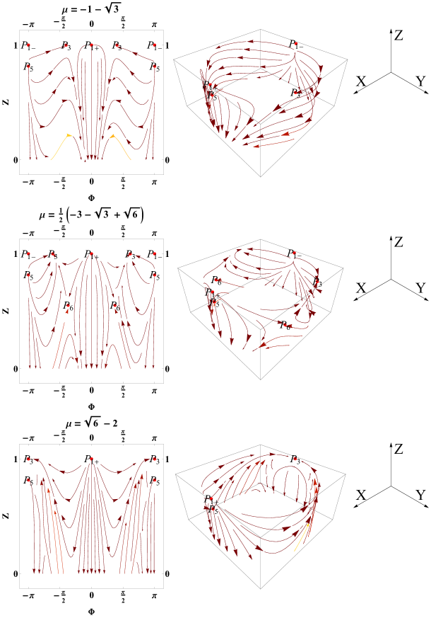
Figure 1: Unwrapped solution space (left panel) and projection over the cylinder $\mathbf{S}$ (right panel) of the solution space of system (69) - (70) for $\mu=-1-\sqrt{3},\frac{1}{2}\left(-3-\sqrt{3}-\sqrt{6}\right),-2+\sqrt{6}$. The region $Z<0$ is nonphysical.

IV.2 Analysis at infinity

In figure 1 are shown some orbits that approaches $Z=0$. The region $Z<0$ is nonphysical. Combining (58) with (62) it follows $r^{2}=x^{2}+y^{2}+\Sigma^{2}\rightarrow\infty$ as $Z\rightarrow 0$.

Therefore, to analyze the dynamics at infinity the following variables $(\rho,u,v)$ are defined:

$$\rho=\frac{r}{1+r},\quad u=\tan^{-1}\left(\frac{\Sigma}{x}\right),\quad v=\tan^{-1}\left(\frac{\sqrt{\Sigma^{2}+x^{2}}}{y}\right),\quad x\in(-\infty,\infty),\quad y\in(0,\infty),\quad\Sigma\in(-\infty,\infty),$$ (71)

such that, $\rho\rightarrow 1$ when $r=\sqrt{x^{2}+y^{2}+\Sigma^{2}}\rightarrow\infty$. The inverse transformation is:

$$x=\frac{\rho}{1-\rho}\cos u\sin v,~{}\Sigma=\frac{\rho}{1-\rho}\sin u\sin v,~{}y=\frac{\rho}{1-\rho}\cos v,\quad u\in\left[0,2\pi\right],\quad v\in\left[0,\frac{\pi}{2}\right].$$ (72)

The solutions are drawn using the coordinates over the Poincaré sphere:

$$\bar{x}=\cos u\sin v,~{}\bar{\Sigma}=\sin u\sin v,~{}\bar{y}=\cos v.$$ (73)

Introducing the time scaling

$$\frac{df}{dT}=\frac{1}{1+r}\frac{df}{d\lambda}\equiv(1-\rho)\frac{df}{d\lambda},$$ (74)

the following dynamical system is obtained:

$$\frac{d\rho}{dT}=\frac{1}{2}(2\rho-1)\left(\rho-2\sqrt{2}(\rho-1)\sin(v)\left(\sin(u)+\sqrt{3}\cos(u)\right)-3\rho\cos(2v)\right),$$ (75)

$$\frac{du}{dT}=\frac{\cos(u)\left(\rho^{2}\cos(v)\cot(v)\left(\sqrt{3}\mu\tan(u)+2\right)+\left(\sqrt{3}\tan(u)-1\right)\csc(v)\left((\rho-4)\rho+\rho^{2}\cos(2v)+2\right)\right)}{\sqrt{2}\rho},$$ (76)

$$\frac{dv}{dT}=-\frac{\cos(v)\left(\sqrt{6}(\rho((\mu+2)\rho-4)+2)\cos(u)+2\sqrt{2}(1-2\rho)\sin(u)-6(\rho-1)\rho\sin(v)\right)}{2\rho}.$$ (77)

As $\rho\rightarrow 1^{-}$, the leading terms are:

$$\frac{d\rho}{dT}=\frac{1}{2}(1-3\cos(2v))+\frac{1}{2}\left(-9\cos(2v)-2\sqrt{2}\left(\sqrt{3}\cos(u)+\sin(u)\right)\sin(v)+3\right)(\rho-1)+O\left((\rho-1)^{2}\right),$$ (78)

$$\frac{du}{dT}=\left(\sqrt{2}\cos(u)\csc(v)+\sqrt{\frac{3}{2}}\left(\mu\csc^{2}(v)-\mu-2\right)\sin(u)\sin(v)\right)$$

$$+\left(\sqrt{2}\cos(u)\csc(v)+\sqrt{\frac{3}{2}}\left(\mu\csc^{2}(v)-\mu-2\right)\sin(u)\sin(v)\right)(\rho-1)+O\left((\rho-1)^{2}\right),$$ (79)

$$\frac{dv}{dT}=\frac{\cos(v)\left(2\sin(u)-\sqrt{3}\mu\cos(u)\right)}{\sqrt{2}}+\frac{1}{2}\cos(v)\left(-\sqrt{6}\mu\cos(u)+2\sqrt{2}\sin(u)+6\sin(v)\right)(\rho-1)+O\left((\rho-1)^{2}\right).$$ (80)

In the limit $\rho\rightarrow 1^{-}$, the radial equation becomes

$$\frac{d\rho}{dT}=\frac{1}{2}(1-3\cos(2v)),$$ (81)

and it is independent of $\rho$. Therefore, the stationary points at infinity are found by setting

$$\sqrt{2}\cos(u)\csc(v)+\sqrt{\frac{3}{2}}\left(\mu\csc^{2}(v)-\mu-2\right)\sin(u)\sin(v)=0,$$ (82a)

$$\frac{\cos(v)\left(2\sin(u)-\sqrt{3}\mu\cos(u)\right)}{\sqrt{2}}=0.$$ (82b)

The stability of the stationary points at infinity is found as follows. First, the stability of the pairs $$(u^{*},v^{*}) u v \rho^{\prime*},v^{*}) \rho^{\prime*},v^{*})>0 \rho=1 \rho^{\prime*},v^{*})<0$$ which satisfy the compatibility conditions (82) are determined in the plane –. Then, the global stability is examined by substituting in (81) and analyzing the sign of . The sign means that the region is approached meaning stability in the radial coordinate, whereas means instability.

In table 1 is offered information about the location and existence conditions of these critical points.

In figure 2, the dynamics of the stationary points at infinity of system (55)-(56) in the plane $(u,v)$ (left panels), where $u$ is the horizontal axis and $v$ the vertical one, and over the Poincarè sphere $\bar{x}=\cos u\sin v,~{}\bar{\Sigma}=\sin u\sin v,~{}\bar{y}=\cos v$ (middle panels) are presented. The axis of the 3D figures are drawn to the right.

Label $:\left(\begin{array}[]{c}u\\ v\end{array}\right)$	$\left(\begin{array}[]{c}\bar{x}\\ \bar{\Sigma}\\ \bar{y}\end{array}\right)$	$\left(\begin{array}[]{c}\rho^{\prime}\\ \lambda_{1}\\ \lambda_{2}\end{array}\right)$	Stability
$Q_{1}:\left(\begin{array}[]{c}\pi\left(2c_{1}+\frac{1}{6}\right)\\ \frac{1}{2}\pi\left(4c_{2}+1\right)\\ \end{array}\right)$	$\left(\begin{array}[]{c}\frac{\sqrt{3}}{2}\\ \frac{1}{2}\\ 0\\ \end{array}\right)$	$\left(\begin{array}[]{c}2\\ -2\sqrt{2}\\ -\frac{2-3\mu}{2\sqrt{2}}\\ \end{array}\right)$	$\begin{array}[]{c}\text{sink for $\mu<\frac{2}{3}$}\\ \text{saddle for $\mu>\frac{2}{3}$}\end{array}$
$Q_{2}:\left(\begin{array}[]{c}\pi\left(2c_{1}+\frac{7}{6}\right)\\ \frac{1}{2}\pi\left(4c_{2}+1\right)\\ \end{array}\right)$	$\left(\begin{array}[]{c}-\frac{\sqrt{3}}{2}\\ -\frac{1}{2}\\ 0\\ \end{array}\right)$	$\left(\begin{array}[]{c}2\\ 2\sqrt{2}\\ \frac{2-3\mu}{2\sqrt{2}}\\ \end{array}\right)$	saddle
$Q_{3}:\left(\begin{array}[]{c}2\pi c_{1}+\tan^{-1}\left(\frac{\sqrt{3}\mu}{2}\right)\\ 2\pi c_{2}+\tan^{-1}\left(\frac{\sqrt{3\mu^{2}+4}}{\sqrt{6\mu-4}}\right)\\ \end{array}\right)$	$\left(\begin{array}[]{c}\frac{2}{\sqrt{3}\sqrt{\mu(\mu+2)}}\\ \frac{\mu}{\sqrt{\mu(\mu+2)}}\\ \frac{\sqrt{2\mu-\frac{4}{3}}}{\sqrt{\mu(\mu+2)}}\\ \end{array}\right)$	$\left(\begin{array}[]{c}2\left(-\frac{4}{\mu+2}+\frac{1}{\mu}+1\right)\\ \frac{(\mu+2)\left(-\mu\sqrt{3\mu^{2}+4}(\mu+2)-\sqrt{-\mu^{2}(\mu+2)\left(3\mu^{2}+4\right)(3\mu(4\mu-3)-2)}\right)}{(\mu(\mu+2))^{3/2}\sqrt{6\mu^{2}+8}}\\ \frac{(\mu+2)\left(\sqrt{-\mu^{2}(\mu+2)\left(3\mu^{2}+4\right)(3\mu(4\mu-3)-2)}-\mu(\mu+2)\sqrt{3\mu^{2}+4}\right)}{(\mu(\mu+2))^{3/2}\sqrt{6\mu^{2}+8}}\\ \end{array}\right)$	$\begin{array}[]{c}\text{saddle for $\mu<\frac{2}{3}$}\\ \text{sink for $\mu>\frac{2}{3}$}\end{array}$
$Q_{4}:\left(\begin{array}[]{c}(2c_{1}+1)\pi+\tan^{-1}\left(\frac{\sqrt{3}\mu}{2}\right)\\ 2\pi c_{2}+\tan^{-1}\left(\frac{\sqrt{3\mu^{2}+4}}{\sqrt{6\mu-4}}\right)\\ \end{array}\right)$	$\left(\begin{array}[]{c}-\frac{2}{\sqrt{3}\sqrt{\mu(\mu+2)}}\\ -\frac{\mu}{\sqrt{\mu(\mu+2)}}\\ \frac{\sqrt{2\mu-\frac{4}{3}}}{\sqrt{\mu(\mu+2)}}\\ \end{array}\right)$	$\left(\begin{array}[]{c}2\left(-\frac{4}{\mu+2}+\frac{1}{\mu}+1\right)\\ \frac{(\mu+2)\left(\mu(\mu+2)\sqrt{3\mu^{2}+4}-\sqrt{-\mu^{2}(\mu+2)\left(3\mu^{2}+4\right)(3\mu(4\mu-3)-2)}\right)}{(\mu(\mu+2))^{3/2}\sqrt{6\mu^{2}+8}}\\ \frac{(\mu+2)\left(\mu\sqrt{3\mu^{2}+4}(\mu+2)+\sqrt{-\mu^{2}(\mu+2)\left(3\mu^{2}+4\right)(3\mu(4\mu-3)-2)}\right)}{(\mu(\mu+2))^{3/2}\sqrt{6\mu^{2}+8}}\\ \end{array}\right)$	saddle

Table 1: Stability of the stationary points at infinity of system (55)-(56). $c_{1}$ and $c_{2}$ are integers.

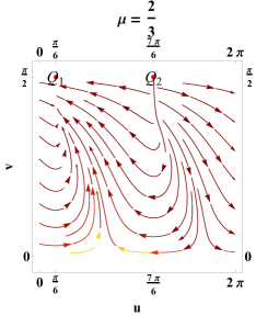
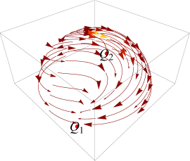
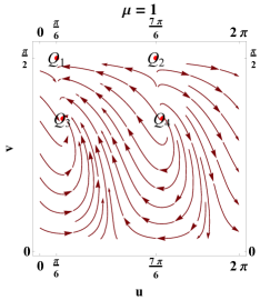
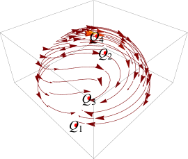
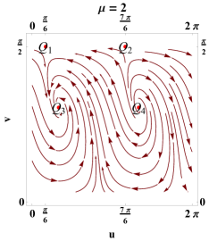
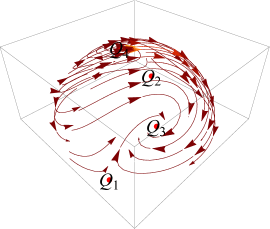
Figure 2: Dynamics of the stationary points at infinity of system (55)-(56) in the plane $(u,v)$ (left panels) and the projection over the Poincarè sphere $\bar{x}=\cos u\sin v,~{}\bar{\Sigma}=\sin u\sin v,~{}\bar{y}=\cos v$ (middle panels).

V Conclusions

In this work in the context of Einstein-Scalar field theory, we determined exact and analytic solutions for the gravitational field equations for a Kantowski-Sachs background spacetime. The gravitational field equations provides three unknown functions which are, the scalar field potential and the coupling functions of the scalar field with the aether field.

For the determination of these unknown functions we apply a geometric selection rule. In particular we require the existence of point transformations which leave the field equations invariants, while from the point transformations we can construct conservation laws, i.e. integrals of motion, such that to simplify the nonlinear field equations and determine the exact solutions.

In addition, the asymptotic behaviour of the field equations is studied, from where we find that the limits of Bianchi I and closed FLRW spacetimes exist. In order to perform a complete and detailed analysis on the determination of the stationary points we work with two different sets of dimensionless variables, the $H$-normalization approach, and the compactification procedure. We observe that the second set of dimensionless variables provides additional information for the evolution of the dynamical system.

In a future work we plan to study by using this approach the case of static spherically symmetric spacetimes and study the existence of black-holes solutions.

References

• (1)  C.W. Misner, The Isotropy of the universe, Ap. J. 151, 431 (1968)
• (2) O. Hrycyna and M. Szydlowski, AIP Conf.Proc. 1514, 191 (2013)
• (3) E. Russel, C. Battal Kilinc and O.K Pashaev, MNRAS 442, 2331 (2014)
• (4) A. Guth, Phys. Rev. D 23, 347 (1981)
• (5) A. Feinstein and J. Ibanez, Class. Quantum Grav. 10, 93 (1993)
• (6) J.M. Aguirregabiria, A. Feinstein and J. Ibanez, Phys. Rev. D 48, 4662 (1993)
• (7) M. Tsamparlis and A. Paliathanasis, Gen. Relativ. Gravit. 43, 1861 (2010)
• (8) T. Christodoulakis, G. Kofinas, E. Korfiatis, G.O. Papadopoulos and A. Paschos, J. Math. Phys. 42, 3580 (2001)
• (9) T. Christodoulakis and P. A. Terzis, Class. Quantum Grav. 24, 875 (2007)
• (10) J. Socorro, L.O. Pimenter, C. Ortiz and M. Aguero, Int. J. Theor. Phys. 48, 3567 (2009)
• (11) M. Thorsud, Class. Quantum Grav. 36, 235014 (2019)
• (12) T. Christodoulakis, T. Grammenos, C. Helias, P.G. Kevrekidis and A. Spanou, J. Math. Phys. 47, 042505 (2006)
• (13) S. Kanno and J. Soda, Phys. Rev. D 74, 063505 (2006)
• (14) W. Donnelly and T. Jacobson, Phys. Rev. D 82, 064032 (2010)
• (15) J.D. Barrow, Phys. Rev. D 85, 047503 (2012)
• (16) A. Paliathanasis, G. Papagiannopoulos, S. Basilakos and J.D. Barrow, EPJC 79, 723 (2019)
• (17) A. Paliathanasis and G. Leon, EPJC 80, 355 (2020)
• (18) A. Paliathanasis and G. Leon, EPJC 80, 589 (2020)
• (19) R. Kantowski and R. K. Sachs, J. Math. Phys. 7, 443 (1966)
• (20) M. Thorsrud, B.D. Normann and T.S. Pereira, Class. Quantum Grav. 37, 065015 (2020)
• (21) S. Byland and D. Scialom, Phys. Rev. D 57, 6065-6074 (1998)
• (22) C. R. Fadragas, G. Leon and E. N. Saridakis, Class. Quant. Grav. 31, 075018 (2014)
• (23) J. Latta, G. Leon and A. Paliathanasis, JCAP 1611, 051 (2016)
• (24) A. A. Coley, G. Leon, P. Sandin and J. Latta, JCAP 12, 010 (2015)
• (25) N. Dimakis, A. Karagiorgos, A. Zampelis, A. Paliathanasis, T. Christodoulakis and P.A. Terzis, Phys. Rev. D 93, 123518 (2016)
• (26) N. Dimakis, P.A. Terzis and T. Christodoulakis, Phys. Rev. D 99, 104061 (2019)
• (27) N. Dimakis, T. Pailas, A. Paliathanasis, G. Leon, P.A. Terzis and T. Christodoulakis, [arXiv:2008.00746]
• (28) T. Christodoulakis, N. Dimakis, P.A. Terzis, G. Doulis, Th. Grammeos, E. Melas and A. Spanou, J. Geom. Phys. 71, 127 (2013)
• (29) T. Christodoulakis, N. Dimakis, P.A. Terzis and G. Doulis, Phys. Rev. D 90, 024052 (2014)
• (30) G. Papagiannopoulos, J.D. Barrow, S. Basilakos, A. Giacomini and A. Paliathanasis, Phys. Rev. D 95, 024021 (2017)
• (31) A. Paliathanasis, M. Tsamparlis, S. Basilakos and J.D. Barrow, Phys. Rev. D 91, 123535 (2015)
• (32) H. Motavali and M. Golshani, IJMPA 17, 375 (2002)
• (33) U. Camci and Y. Kucukakca, Phys. Rev. D 76, 084023 (2007)
• (34) J. Mubasher, F.M. Mahomed and D. Momeni, Phys. Lett. B 702, 315 (2011)
• (35) Y. Zhang, Y.-G. Gong, Z.-H. Zhu, Phys. Lett. B 688, 13 (2010)
• (36) H. M. Sadjadi, Phys. Lett. B 718, 270 (2012)
• (37) B. Vakili, F. Khazaie, Class. Quant. Grav. 29, 035015 (2012)
• (38) B. Modak, S. Kamilya and S. Biswas, Gen. Relativ. Gravit. 32, 1615 (2000)
• (39) A. Paliathanasis, M. Tsamparlis and S. Basilakos, Phys. Rev. D 84, 123514 (2011)
• (40) J.A. Belinchon, T. Harko and M.K. Mak, Astroph. Sp. Sci. 361, 52 (2016)
• (41) C. B. Collins, J. Math. Phys. 18, 2116 (1977)
• (42) E. Weber, J. Math. Phys. 25, 3279 (1984)
• (43) O. Gron, J. Math. Phys. 27, 1490 (1986)
• (44) D. Lorenz-Petzold, Phys. Lett. B 149, 79 (1984)
• (45) D. M. Solomons, P. Dunsby and G. Ellis, Class. Quant. Grav. 23, 6585 (2006)
• (46) S. Jamal and G. Shabbir, Eur. Phys. J. Plus 132, 70 (2017)
• (47) M. Zubair and S. M. Ali Hassan, Astrophys. Space Sci. 361, 149 (2016)
• (48) F. G. Alvarenga, R. Fracalossi, R. C. Freitas and S. V. B. Gonçalves, Braz. J. Phys. 48, 370 (2018)
• (49) J. D. Barrow and M. P. Dabrowski, Phys. Rev. D 55, 630 (1997)
• (50) U. Camci, A. Yildirim and I. Basaran Oz, Astropart. Phys. 76. 29 (2016)
• (51) J. D. Barrow and A. Paliathanasis, Eur. Phys. J. C 78, 767 (2018)
• (52) S. Calogero and J. M. Heinzle, Physica D 240, 636 (2011)
• (53) B. J. Carr and A. A. Coley, Phys. Rev. D 62, 044023 (2000)
• (54) M. de Cesare, S. S. Seahra and E. Wilson-Ewing, JCAP 07, 018 (2020)
• (55) D. Clancy, J. E. Lidsey and R. K. Tavakol, Class. Quant. Grav. 15, 257 (1998)
• (56) R. Chan, M.F.A. da Silva and V.H. Satheeshkumar, The General Spherically Symmetric Static Solutions in the Einstein-Aether Theory, [arXiv:2003.00227]
• (57) B. Alhulaimi, R.J. van den Hoogen and A.A. Coley, JCAP 17, 045 (2017)
• (58) R.J. van de Hoogen, A.A. Coley, B. Alhulaimi, S. Mohandas, E. Knighton and S. O’Neil, JCAP 18, 017 (2018)
• (59) A. Coley and G. Leon, Gen. Rel. Grav. 51, no. 9, 115 (2019)
• (60) G. Leon, A. Coley and A. Paliathanasis, Annals Phys. 412, 168002 (2020)
• (61) S. Basilakos, M. Tsamparlis and A. Paliathanasis, Phys. Rev. D 83, 103512 (2011)
• (62) L.V. Ovsiannikov, Group Analysis of Differential Equations, Academic Press, New York (1982)
• (63) M. Tsamparlis and A. Paliathanasis, Symmetry 10, 233 (2018)