Analysis of soliton gas with large-scale video-based wave measurements

Abstract

An experimental procedure for studying soliton gases in shallow water is devised. Nonlinear waves propagate at constant depth in a 34 m-long wave flume. At one end of the flume, the waves are generated by a piston-type wave-maker. The opposite end is a vertical wall. Wave interactions are recorded with a video system using seven side-looking cameras with a pixel resolution of 1 mm, covering 14 m of the flume. The accuracy in the detection of the water surface elevation is shown to be better than 0.1 mm. A continuous monochromatic forcing can lead to a random state such as a soliton gas. The measured wave field is separated into right- and left-propagating waves in the Radon space and solitary pulses are identified as solitons of KdV or Rayleigh types. Both weak and strong interactions of solitons are detected. These interactions induce phase shifts that constitute the seminal mechanism for disorganization and soliton gas formation.

1 Introduction

A soliton gas is one of the possible random statistically stationary state of water wave motions. It is described by the theory of integrable turbulence (Zakharov, 1971, 2009), one of the theories along with the weak wave turbulence (Hasselmann, 1962; Nazarenko, 2011) developed to describe the interaction of weakly nonlinear dispersive and random waves. Integrability of the equations exhibiting soliton solutions means that an infinite number of quantities amongst which mass, momentum, energy are conserved in time. It also implies that nonlinear coherent structures (such as solitons) emerge from any initial condition. A soliton gas is the statistical state in which solitons have random distributed amplitudes and phases. Not only integrable turbulence poses theoretical and experimental challenges in itself but is also one of the keys to understanding sea states generation and characteristics in shallow ocean basins (Costa et al., 2014).

Solitons are fascinating objects that propagate in weakly dispersive media. Since the first experimental observations of Scott-Russell (1844) many other experiments have been reported in the literature (e.g. Hammack and Segur, 1974; Seabra-Santos et al., 1987). In the framework of water waves in shallow water, solitons are solutions of nonlinear equations such as the Korteweg-de Vries (KdV) equation (Korteweg and de Vries, 1895). The KdV equation models a balance between non-linear and dispersive effects that shapes a solitary pulse of permanent form. Nonlinear effects steepen wave fronts while frequency dispersion stretches wave crests with components at different frequencies traveling with different speeds. The free surface displacement due to a propagating soliton, also referred to as a solitary wave, is

$$\eta=a_{s}\ {\rm sech}^{2}\left[\frac{\beta}{2}\left(x-c\,t\right)\right]\,,$$ (1)

where $\eta$ is the water surface elevation, $a_{s}$ the amplitude of the soliton, $c$ the phase speed, $\beta$ the shape factor, $x$ the space coordinate and $t$ time. The soliton is a localized symmetric hump traveling at constant speed. The parameters of this KdV solution fulfill

$$c=c_{\rm K}=\sqrt{gh}\left(1+\frac{a_{s}}{2h}\right)$$ (2)

and

$$\beta=\beta_{\rm K}=\sqrt{\frac{3a_{s}}{h^{3}}}\,,$$ (3)

where $h$ is the quiescent water depth and $g$ the gravity acceleration. The $\beta$ parameter is a measure of the exponential decay of the trailing edges of the soliton. The non-dimensional expression is

$$\beta^{*}_{\rm K}=\beta_{\rm K}\,h=\sqrt{\frac{3\,a_{s}}{h}}\,.$$ (4)

The shallow water KdV approximation assumes both long waves and small amplitude. Relaxing the latter restriction of small amplitude, an alternate solution known as the Rayleigh solitary wave solution is

$$c=c_{\rm R}=\sqrt{g\left(a_{s}+h\right)}$$ (5)

and

$$\beta=\beta_{\rm R}=\sqrt{\frac{3\,a_{s}}{h^{2}\left(a_{s}+h\right)}}=\frac{\beta_{K}}{\sqrt{1+{a_{s}}/{h}}}\,.$$ (6)

The Rayleigh solitary waves decay more gradually in the trailing edges than those of KdV: they are wider.

The experimental generation of soliton gases is challenging. These random states emerge on very long time scales and thus require long-term experiments. Very recently Redor et al. (2019), drawing on the fission of sine-type long waves into multiple solitons (Zabusky and Galvin, 1971; Trillo et al., 2016), used a continuous wave-maker forcing in order to reach a soliton gas state, such a state only obtained numerically so far (e.g. Pelinovsky and Sergeeva, 2006; Carbone et al., 2016). The wave generation set-up is similar to that used by Ezersky et al. (2009) but in a longer flume in order to favor sine-wave complete fission into solitons. A piston-type wave maker is driven with a small regular motion at one end and the waves are free to reflect against a vertical wall at the other end. Reflection of solitons, dynamically equivalent to head-on collisions (Renouard et al., 1985; Chen and Yeh, 2014), that also occur in the experiments produce soliton amplitude reduction, dispersive wave generation and phase shifting (see also Chen et al., 2014, for a thorough analysis of the flow field). Strong interaction (overtaking collision) also induces a phase shift to the solitons (e.g. Umeyama, 2017). These many collisions of the two types concur to the emergence of a bi-directional soliton gas. Soliton amplitude random distribution is also a result of the dissipative decay due to friction as modeled by Keulegan (1948) with a boundary layer model.

The randomness and bi-directionality of the wave field makes it difficult to track the solitons traveling back and forth. Even though arrays of closely arranged wave probes and repeated experiments to cover large regions of interest (e.g. Taklo et al., 2017) are possible, actual improvements in video resolution provide image based measurements with sufficient spatial resolution to separate waves traveling in both directions. Video techniques such as slope detection and relative brightness for statistical properties of wave fields (Zhang and Cox, 1994; Chou et al., 2004), bichromatic synthetic Schlieren (Kolaas et al., 2018), free surface synthetic Schlieren (Moisy et al., 2009) and Fourier transform profilometry (Cobelli et al., 2009; Aubourg and Mordant, 2016), are widely used to measure 2D water wave motions. Bonmarin et al. (1989) used a side-looking CCD camera to image the interface in breaking waves in a 1D wave flume. The technique relies on tinted water and sharp lighting to create strong contrasts at the interface amenable to edge detection processing. Although the foundations of this technique with coarse resolution are close to those described in this paper, it was only used to measure one wave length. Recent technologies allow for multiple synchronized camera settings and large redundant storage capacities as presented hereafter. The innovative system used for this study images a $14$-m-long section of a $34$-m-long flume with sub-millimetric resolution, enabling to capture highly nonlinear wave interactions in random states. In addition, we use the Radon transform (Deans, 2007) to separate, in the space-time field, the direction of propagation of the solitons and to determine their phase speed. As shown by Sanchis and Jensen (2011) for instance, the Radon transform is well suited to the detection of lines in noisy images.

The experimental set-up is described in detail in Redor (2019), we recall the main characteristics in section 2. Measurement accuracy, wave separation methods, analysis of soliton head-on collision and soliton dissipation, are presented in section 3. The soliton gas experiments are described and analyzed in section 4. Section 5 is devoted to the conclusions.

2 Experimental set-up

Figure 1: View of a section of the flume, with one of the cameras (bottom right corner). Each camera records the water surface elevation along the 1.92 m separating two vertical beams (red-brownish color).

2.1 Wave flume

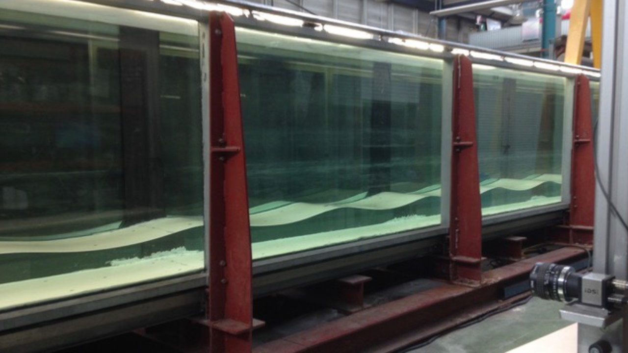
The flume is horizontal within a few millimeters over its entire length $L=33.73$ m. Its width is $l=0.55$ m. The flume is made of lateral glass windows of 1.92-m-long maintained together by steel cradles with vertical beams 8-cm-wide (see Figure 1).

The left-hand boundary of the flume is a movable vertical piston-type wave-maker of 0.6 m maximum stroke. It is controlled in position, with an accuracy of approximately 1 mm, to produce any prescribed motion of limited acceleration (roughly frequencies $f\leq 2$ Hz). Following Guizien and Barthélemy (2002), solitons with minimum trailing dispersive tail can be generated according to Rayleigh’s law of motion, i.e. a single forward push of tanh shape. In the present paper, we consider interactions between solitons. Producing several solitons with Rayleigh’s law implies to move back the piston before each new forward push. To overcome this limitation, solitons can be produced through nonlinear steepening of a regular monochromatic forcing of large enough amplitude, as shown in section 4.

2.2 Video

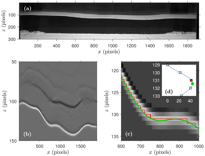
In most experiments, the water elevation is recorded at 20 frames/s (maximum 100 fps) with seven cameras located 2 m aside of the flume (see Figure 1) covering seven glass windows 1.92 m long. The flume bottom is painted white and the background wall is black. The flume is illuminated from above the free surface. Each camera is slightly downward-looking the water surface. This provides the best contrast for following the water surface along the front glass wall. An example of a raw image is shown in Figure 2(a). The image size is $1936\times 300$ pixels, so that the pixel resolution is about one square millimeter. Pictures of a regular grid are used for calibration (see e.g. Tsai, 1987).

The region of interest is automatically detected to remove the flume beams and flume bottom. A first estimation of the interface position is the line of pixels of maximum gray level gradient, see Figure 2(b). Sub-pixel resolution is achieved by fitting a $4^{\rm th}$ order polynomial curve in the gray level gradient over a vertical column of five pixels, see Figure 2(d). The maximum of that curve provides the interpolated interface position, see Figure 2(c).

Many other proxies for interface position have been tested, such as darkest or brightest pixels. The method described above appears to be the best for minimizing bias or hysteresis related to glass wall capillary meniscus, as will be shown in the following.

Figure 2: (a) Snapshot of a camera field of view in $2^{8}$ gray levels. The bright regions are the bottom of the flume and the water surface, seen with a slight down-looking angle. (b) Region of interest in gray level gradient. (c) Close-up with detected maximum gradient (red line) and interpolated interface (green line). (d) Vertical profile, at $x=800$ pixels, of the gray level gradient (squares), with maximum (filled square), $4^{\rm th}$ order polynomial best fit (solid line) and interpolated interface position (green dot).

3 Wave analysis

3.1 Water drop experiment

Figure 3: The water drop experiment. (a) Time-space representation of the free surface elevation in the field of view of the last camera (drop injection is at $x=0$). (b) Time series extracted from (a) at $x=22.5$ m. (c) $E(k,\omega)$ spectrum computed from the full field of view ($9.53\leq x\leq 23.45$ m) with a 0.08 m resolution. (d) Same as (c) with superimposed dispersion relations : linear waves propagating along $x$ (dashed) and combined waves (dotted) related to resonant transverse modes (the three first ones are marked with circles).

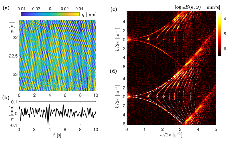
In order to assess the accuracy of the free surface detection procedure and measurement, the following experiment is conducted. The flume is filled at a water depth of $h=0.7$ m. At one end of the flume a small vertical tube drips, releasing water drops that impact the water surface every 5 to 10 s. The waves generated by the successive impacts are recorded with the cameras. An example of the free surface elevation record is shown in Figure 3(b), for which the standard deviation of the free surface displacement is a few hundredths of millimeter. In the space-time field in Figure 3(a) the color ridges are the signature of waves crests and troughs that essentially propagate from left to right in the flume.

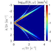
The 2D Fourier spectrum shown in Figure 3(c) for this experiment is computed over the full 14-m-long field of view as the square modulus of the time-space Fourier transform $\tilde{\eta}(k,\omega)$:

$$E(k,\omega)={\left|\int\!\!\!\!\int\eta(x,t)e^{i(kx+\omega t)}\mathrm{d}x\mathrm{d}t\right|}^{2}\,.$$ (7)

For $\omega>0$, negative wave numbers $k<0$ correspond to waves propagating with increasing $x$ (similarly for $\omega<0$ and $k>0$ as the field is real), while $k>0$ represent waves reflected by the flume end-wall for $0<\omega/2\pi<3$ s^-1. Due to spectral aliasing (in wave number) for this spatial resolution of 8 cm, the energy for $k>0$ and $\omega/2\pi>3$ s^-1 corresponds to waves propagating towards the end-wall.

The energy in the ($k,\omega$) plane is mostly located along curves, see Figure 3(d). On the one hand waves propagating along the $x$ axis in both directions match the dispersive relation of linear waves:

$$\omega=\pm(gk\tanh(kh))^{1/2}\,.$$ (8)

On the other hand the wave numbers of resonant transverse modes with anti-nodes at the lateral walls match

$$k_{y}=\frac{\pi n}{l}\quad{\rm with}\quad n\in\mathbb{N}\,.$$ (9)

These transverse waves correspond to dots along the $k=0$ axis with $\omega=(gk_{y}\tanh(k_{y}h))^{1/2}$. Their interactions with waves propagating along $x$ produce transverse waves that comply the following dispersive relation:

$$\omega=\left(g\left(k^{2}+{k_{y}}^{2}\right)^{1/2}\tanh\left(\left(k^{2}+{k_{y}}^{2}\right)^{1/2}h\right)\right)^{1/2}\,.$$ (10)

The good agreement of the measurements with these theoretical estimators indicates that the accuracy of the video sub-pixel detection can be of the order of a few hundredths of a millimeter.

3.2 Wave separation

(a)                                           (b)                                   (c)

Figure 4: Head-on collision of two solitons: water surface elevation (a) and separated right-running waves (b), time-space Fourier spectrum (c): in dashed is the linear dispersion relation (8), in solid is the relation $\omega=\pm c_{0}k$. Water depth: $h=12$ cm, right-running soliton amplitude: $a_{+}=4.7$ cm, left-running soliton amplitude: $a_{-}=5.0$ cm.

3.2.1 Fourier transform

In order to get a better understanding of wave interactions in the bidirectional flow, waves propagating towards positive $x$ (’right-running’) can be separated from those propagating towards negative $x$ (’left-running’) by computing the inverse Fourier transform of selected quadrants of the time-space spectrum computed with (7). An example is shown in Figure 4. Figure 4(c) is the time-space spectrum of the interaction of two solitons propagating in opposite directions. The time-space field of surface elevation is plotted in Figure 4(a). The signatures of the two solitons are identified as the bright straight lines. Waves with $k<0$ and $\omega>0$ propagate towards positive $x$ and waves with $k>0$ and $\omega>0$ to negative $x$. The energy in Figure 4(c) is mostly located along straight lines, which confirms that all the frequency components of each soliton propagate at the same speed $c=\left|\omega/k\right|>c_{0}$, where $c_{0}=\sqrt{gh}$ is the linear long wave phase speed. Weaker energy levels are located along the dispersion relation of linear waves (8) which is the signature of weak dispersive waves. Applying the inverse Fourier transform on $\tilde{\eta}(k<0,\omega>0)$ produces the field shown in Figure 4(b). Small amplitude dispersive waves are visible in the top-left corner of the plot, corresponding to waves generated in the lee of the soliton by the wave-maker motion. Additional small waves are generated at the collision.

3.2.2 Radon transform

An alternative to the Fourier transform for separating right- and left-running waves is the Radon transform (Deans, 2007; Almar et al., 2014). The Radon transform is the projection of a field intensity along a radial line oriented at a specific angle $\theta$:

$$R(\rho,\theta)=\int\!\!\!\!\int\eta(x,t)\,\delta\!\left({\frac{x}{\Delta x}}\cos\theta+{\frac{t}{\Delta t}}\sin\theta-\rho\right)\,\mathrm{d}x\,\mathrm{d}t$$ (11)

where $\delta$ is the Dirac function and $\rho=((x/\Delta x)^{2}+(t/\Delta t)^{2})^{1/2}$ is the distance (in pixels, with $\Delta x$ and $\Delta t$ the spatial and temporal resolutions, respectively) from origin (center of the two-dimensional field).

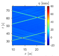
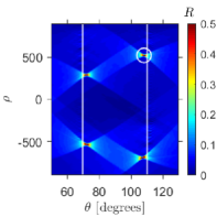
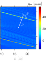
For example, we consider the $\eta(x,t)$ field shown in Figure 5(a) of two solitons passing twice in front of the cameras. Four local maxima are detected in the Radon space shown in Figure 5(c). These four maxima correspond to the four crest trajectories of the $\eta(x,t)$ field in Figure 5(a). The local maxima $\theta$ values correspond to the propagation speed of the four solitons. Applying the inverse Radon transform on $R_{-}=R(\rho,\theta>90^{\circ})$ produces the plot in Figure 5(b) where only left-running waves are reconstructed. Note that the local maxima $\theta$ values for the left-running waves are below the $\theta_{0}$ associated to $c_{0}$, confirming that the solitons travel faster than $c_{0}$.

(a)                                           (b)                                   (c)

Figure 5: Two head-on collisions of two solitons (same experiment as in Figure 4): (a) water surface elevation and (b) separated left-running waves, (c) projection of $\eta(x,t)$ in the Radon space $R(\theta,\rho)$. The angle $\theta$ is the inclination relatively to the vertical axis in the $(x,t)$ plane, $\rho$ is the distance to the center of the field $\eta(x,t)$, as drawn in (b) for the local maximum marked with a circle in (c). The vertical lines are angle values $\theta_{0}=69.8^{\circ}$ and $110.2^{\circ}$ that both correspond to $c_{0}=1.07$ m s^-1 in the physical space $(x,t)$.

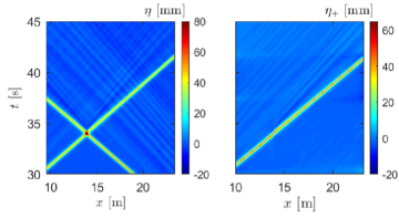
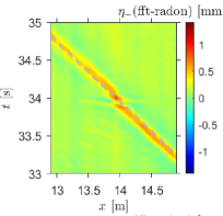
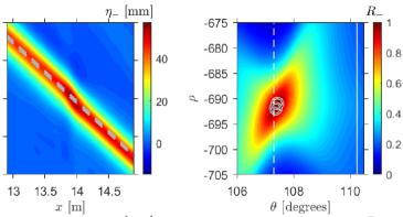
Fourier and Radon separation methods give similar results. For instance, we compare the reconstructed fields of the soliton head-on collision. The difference between left-running reconstructed fields is shown in Figure 6(a) to be less than 1 mm. The focus on this left-running separated wave shown in Figure 6(b) highlights the phase lag that a soliton undergoes during a head-on collision. Indeed the color ridges before and after the collision are not aligned. Moreover both separation methods assign a part of the overall amplitude amplification due to non-linearity ($\eta_{\max}>a_{+}+a_{-}$, with $a_{+}$ and $a_{-}$ the amplitudes of the right- and left-running solitons, respectively) to each of the solitons, as will be discussed in more detail below in section 3.3.

The corresponding signature in the Radon space $R_{-}(\rho,\theta>90^{\circ})$, in Figure 6(c), exhibits two local maxima that correspond to waves propagating at a roughly same constant speed in the physical plane, emphasized by dashed lines in Figure 6(b). They are associated to the soliton trajectory before and after the head-on collision. Their speeds are very close to that of a KdV or Rayleigh soliton of amplitude $a=0.4\,h$. This example emphasizes that the Radon transform is also a tool for identifying soliton trajectories, their speeds and eventually phase shifts.

(a)                                           (b)                                   (c)

Figure 6: Close-up of the left-running soliton in the head-on collision shown in Figure 5(a) at ($x=14$ m, $t=34$ s): (a) difference between separated left-running wave fields from Fourier and Radon, (b) left-running wave, (c) corresponding signature in the Radon space $R_{-}(\theta,\rho)$. The vertical solid line corresponds to $c_{0}$, the vertical dashed line corresponds to the speed (5) of a Rayleigh soliton of amplitude $a=0.4h$. Two detected local maxima are marked with circles, their transposition into the physical space $(x,t)$ are marked as dashed lines in (a,b) and correspond to the soliton before and after interaction.

Figure 7: Head-on collision of two solitons: water surface elevation (dotted) separated into right-running soliton (red) and left-running soliton (green). Gray solid lines are KdV profiles matching the measures at the beginning of the collision (top panel), gray dashed lines are Rayleigh profiles matching the measurements 1 s after collision (bottom panel). During the collision (second panel) note a nonlinear amplification resulting in a maximum free surface elevation exceeding the linear superposition of the two incident waves, as shown by the inserts. The interaction is inelastic, characterized by asymmetric wave profiles at the end of the collision (third panel) and the generation of dispersive waves in the lee of each soliton.

3.3 Weak interaction of two solitons

Free surface elevation time series of the head-on collision of the experiment of Figure 5 are shown in Figure 7. The measured profiles are in fair agreement with theoretical KdV profiles (3) before and long after the collision. During the collision the separated solitons are stretched, so that the measured maximum surface elevation exceeds that of the sum of the incoming soliton amplitudes. In this example, the conditions ($a_{+}/h=a_{-}/h=0.4$) are similar to that of Chen and Yeh (2014) and the maximum amplification is $\eta_{\max}/(a_{+}+a_{-})=1.13$ too. Just after the collision, before the dispersive tails detach from the solitons, the measured wave profiles tally more closely to the Rayleigh soliton profiles (6).

Figure 8: Time series of water surface elevation (dotted) separated into right-running wave (red) and left-running wave (green). Gray solid lines are KdV profiles, gray dashed are sech² fitted profiles. Same experiment as in Figure 7.

In the same experiment, the two solitons continue to propagate back and forth in the flume, reflecting at both ends and interacting. Even for large propagation durations solitary waves pulses matching a sech² profile (1) are still detected (see Figure 8). The solitary waves in Figure 8 have traveled 7 times back and forth and the waves are a few tenths of a mm high. The dashed gray lines represent solitons (1) with 3 fitted parameters $a$, $\beta$ and $h_{r}$, the latter parameter $h_{r}$ accounting for a soliton propagation at a reference level different than $h$. The fitted shape factor $\beta$ is here larger than that of the KdV solution (3), meaning that the measured solitons are narrower. This is probably due to the weak background flow induced by the wave-maker backward slow motion (after each forward push that produces a soliton) that generate a standing seiching wave. At long times, each soliton is leading a remnant long wave crest propagating at $c_{0}$ too. This also corresponds to $h_{r}<h$ of about one tenth of a mm just in front of each leading soliton in Figure 8.

All the elements discussed in this section indicate that our video system can accurately capture nonlinear wave dynamics. Automatic detection of wave crests and their propagation speed with the Radon transform is a tool to determine soliton characteristics in a wave field.

3.4 Adiabatic soliton propagation

(a)                                                           (c)
                    
             (b)                                                           (d)

Figure 9: Time variations of crest (a) maximum and (b) speed detected at $x=17$ m. The horizontal line is $c_{0}=1.07$ m s^-1, the red dashed lines represent Keulegan’s dissipation decay laws. (c) Dimensionless speed against dimensionless amplitude and (d) dimensionless shape factor $\beta_{*}=\beta hc/c_{0}$ against dimensionless soliton amplitude. Thick solid and dashed lines are for KdV and Rayleigh solutions, respectively. Right (left) pointing triangles are for right (left) propagating waves. Small triangles correspond to a single soliton traveling back and forth in the flume. Large triangles correspond to the head-on collision experiment.

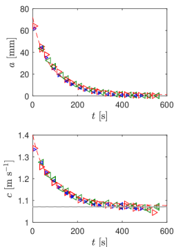
The time evolution of soliton amplitude and speed is plotted in Figure 9(a, b), for the head-on collision experiment described above as well as for a single soliton propagating back and forth in the flume. Both amplitude and speed decays show good agreement with the boundary layer dissipation decay laws proposed by Keulegan (1948).

The soliton profiles match well nonlinear theoretical solutions, with best fit parameters lying in between KdV and Rayleigh solutions, as measured at the middle of the flume and plotted in Figure 9(c,d) for instance.

Despite dissipation, the solitons propagating back and forth in the flume closely fulfill at any time a balance between dispersive and non-linear effects. In that sense the soliton propagation can be considered adiabatic, and thus integrable.

4 Soliton gas

(a)                                          (b)                                          (c)

    (d)                                          (e)                                          (f)

    (g)                                          (h)                                          (i)

Figure 10: Space-time surface elevation (a-c), space-time Fourier spectrum after 20 min of forcing (d-f) with solid lines indicating $\omega=c_{0}\left|k\right|$ and dashed lines for the dispersion relation (8), and time variation of the spatial spectrum (g-i). Water depth $h=12\,$cm ($c_{0}=1.07\,$m/s), sinusoidal forcing with frequency $\omega/2\pi=0.6$ s^-1 and amplitude $a_{0}=4$ mm (a,d,g), $a_{0}=6$ mm (b,e,h), $a_{0}=12$ mm (c,f,i).

In the previous section the measuring system was validated along with the processing tools adapted to nonlinear wave propagation. Hereafter we describe and analyze, in particular on large time scales, the wave field generated by a continuously right-running sinusoidal wave. The flume water depth is $h=12$ cm, the sinusoidal wave surface elevation is $\eta(x=0,t)=a_{0}\sin(\omega_{0}t)$, with $\omega_{0}/2\pi=0.6$ s^-1. Three different forcing amplitudes are considered: $a_{0}=4$, 6 and 12 mm. The waves are free to reflect at both ends of the flume.

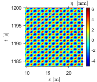
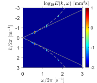
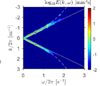
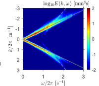
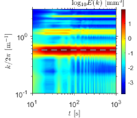
Figure 10(a-c) shows space-time representations of the wave field after 20 minutes for the three cases. For the smallest amplitude plotted in Figure 10(a), a steady state is reached exhibiting a standing wave pattern. This is confirmed by the space-time spectrum in Figure 10(d) where the energy is mainly located at the forcing frequency and its harmonics $2\omega$ and $3\omega$. Figure 10(g) is the time variation of the spatial spectrum for the same experiment, indicating that the steady state is rapidly reached, say after about 200 s or a few flume-length travels of the first wave train. Of note, the two red ridges for $10<t<100$ s for $k/2\pi=1.15$ m^-1 and $1.26$ m^-1 corresponding to both bound and free second harmonic, respectively.

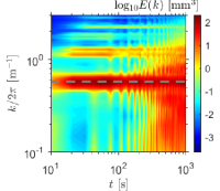
For a slightly larger forcing ($a=6$ mm), the evolution is very similar during the first 100 s, see Figure 10(h). At later times, energy is distributed over a wider range of wave numbers. After 20 minutes of forcing, two red spots at the main frequency $\omega_{0}/2\pi=0.6$ s^-1and $k_{0}/2\pi=\pm 0.58$ m^-1 are clearly visible in Figure 10(e), but energy located along the straight lines $\omega/k=\pm c_{0}$ denotes the presence of solitons. The corresponding wave field (Figure 10b) is characterized by bright ridges that are the signature of solitons propagating at various speeds.

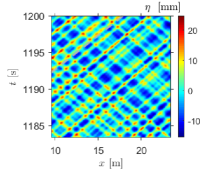
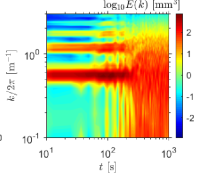
These features are even more obvious for the larger forcing amplitude $a=12$ mm in Figure 10(c, f, i). Energy is distributed over a large frequency band, see Figure 10(f), with no dominance of the forcing frequency after 300 s of experiment as shown in Figure 10(i).

A closer inspection of Figure 10(h, i) gives a clue for understanding the mechanisms of soliton gas outbreak. The energetic wave number band around $k_{0}$ is bleeding every $\sim 30$ s (appearing as vertical streaks). This period corresponds to the return time, in the field of the cameras, of the remnant wave front initiated at the start of the wave-maker motion. This periodic spectral bleeding, characterized by energy increase on a larger wave-number band, is enhanced each time the front returns. 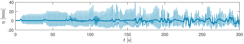At some point the system bifurcates to a white noise type of random wave field. 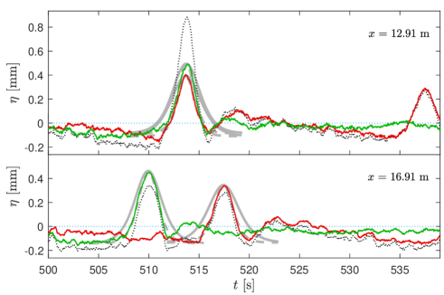This is illustrated in Figure 11. The reflected solitons that emerged from the first wave front favorably interact with those emerging from the freshly generated sine waves. This generates phase shifts that randomize the wave field after a few cycles. The low-pass filtered signal plotted in Figure 11 underlines the progressive outbreak of low frequency wave components.

Figure 11: Time series of free surface elevation (thin line) and low-pass-filtered (thick line) recorded at the middle of the flume $x=16.89$ m. Water depth $h=12$ cm, sinusoidal forcing with frequency $\omega/2\pi=0.6$ s^-1 and amplitude $a_{0}=12$ mm.

(a)                                          (b)                                          (c)
                                                      (d)                                          (e)
                                               

Figure 12: (a) Close-up of a soliton gas wave field with separated (b) right-going waves and (d) left-going waves. Dashed gray lines are crests identified from local maxima (circles in c,e) in the Radon space. Corresponding crest speeds are close to $c_{0}$ (vertical solid lines in c,e). Several soliton interactions are observed in (a), in particular a weak interaction at ($x=13.7$ m, $t=1146$ s), a strong interaction of right-going solitons centered at ($x=14.8$ m, $t=1147$ s).

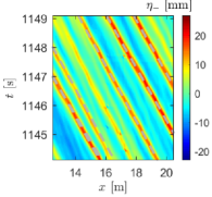
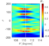
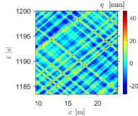
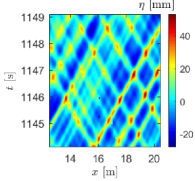
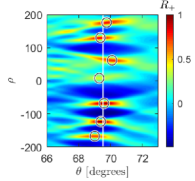
Figure 12 provides a selected part of the wave field for the largest forcing amplitude that emphasizes nonlinear interactions in the gas. The local maxima in the Radon space shown in Figure 12(c, e) indicate that the waves propagate at speeds close to $c_{0}$, with some random scatter. The separation into right- and left-running waves evidences soliton interactions. A weak interaction or head-on collision with associated phase shifts is observed at ($x=13.7$ m, $t=1146$ s). The same right-running soliton is overtaking a slower propagating soliton around ($x=14.8$ m, $t=1147$ s) with characteristics of a strong interaction. The fastest soliton is shifted ahead and the center of the interaction exhibits a two-heads feature. Another strong interaction of right-running solitons can be seen around ($x=13.2$ m, $t=1147.2$ s) with a quasi-simultaneous weak interaction with a left-running soliton. For this small (8 m, 5 s) selected region, at least 3 strong interactions and about 24 weak interactions can be identified. This underlines that many soliton interactions occur in the gas.

Figure 13: Snapshots of surface elevation (dotted) separated into right-going waves (red) and left-going waves (green). Gray solid lines are KdV profiles, black dashed are sech² fitted profiles that closely match the KdV profiles. The arrows mark the leading soliton of the strong interaction shown in Figure 12(b).

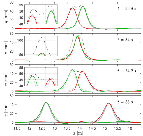
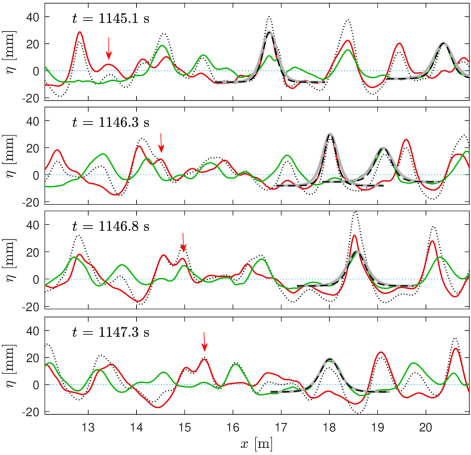
The data processing presented in section 3 is applied in order to evaluate soliton characteristics in the gas. An arbitrary criterion is defined on the standard deviation of the difference between the measured profile and a sech² fit. This enables us to identify symmetric soliton-type pulses but excludes the identification of the solitons during strong interactions. Snapshots of surface elevation at four different times are shown in Figure 13. It provides an alternate view (for $x<16$ m) of the overtaking interaction described above. On the right-hand side of the figure, counter propagating solitons with superimposed fitted profiles are seen to collide in the third panel at ($x=18.5$ m, $t=1146.8$ s). Here the detected pulses match KdV theoretical profiles. In particular, the left-running pulse at $x=20.3$ m that just entered the range of the plot (top panel) complies to a soliton KdV shape through the interaction. It is noteworthy that the fitting evidences that the solitons propagate on a reference level $h_{r}$ that is below the quiescent water level $h$.

(a)                                                           (c)
                    

             (b)                                                           (d)

Figure 14: Time variations of crest (a) maximum and (b) speed detected at $x=16.9$ m with the Radon transform. The thin solid gray line is $c_{0}$, the black dashed line is $\omega/k$ fulfilling the dispersion relation (8) with $\omega/2\pi=0.6$ s^-1. (c) Dimensionless speed by the Radon transform against dimensionless amplitude and (d) shape factor against dimensionless detected soliton amplitude. Thick solid and dashed lines are for KdV and Rayleigh solutions, respectively. Right (left) pointing triangles are for right (left) running waves. Water depth $h=12$ cm, sinusoidal forcing with frequency $\omega/2\pi=0.6$ s^-1 and amplitude $a_{0}=4$ mm (cyan), $a_{0}=6$ mm (red), $a_{0}=12$ mm (green). In (d), only detected solitons with $a_{s}>2\,a_{0}$ are shown.

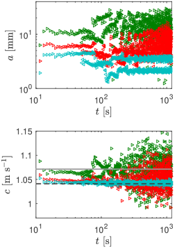
The time evolution of crest maximum, detected in the middle of the flume with the Radon transform over a sliding temporal window, is plotted in Figure 14(a), for three different amplitudes of the monochromatic forcing. For times $t<50$ s, only right-running waves are present. Waves reflected by the end wall recorded thereafter have a weaker amplitude due to dissipation. The combination of waves reflected by the wave-maker with newly produced waves are recorded after 75 s. Amplification in crest maximum is then observed for the largest forcing $a_{0}=12$ mm but the waves remain relatively organized until $t\sim 120$ s. Afterward wave crests reach various maxima, some exceeding 2.5 times $a_{0}$. Apparently randomized crest maxima is one of the soliton gas feature. A similar trend is obtained for $a_{0}=6$ mm, yet for a delayed and more progressive disorganization. In contrast, crest variability is small for the smaller forcing.

The time evolution of detected crest speed is shown in Figure 14b. For the smaller amplitude of forcing, the wave speed complies to the intermediate water depth phase velocity $c=\omega/k$ with (8) for the entire 20 minutes experiment (except for the very first waves that are at the front of the long wave produced by the departure from rest of the wave-maker), within an error range of about 5 mm s^-1 or 0.5 % of $c$. This is an indication of the accuracy of speed estimation with the Radon transform.

The wave speed of the first waves is increasing with increasing forcing amplitude $a_{0}$. For the largest forcing, the right-running wave crests propagate faster than $c_{0}$ for $75<t<120$ s which is a clear signature of soliton behavior. Subsequent disorganization characterized by a strong scattering of propagation speeds is the consequence of the multiple soliton interactions and the scattering of solitons amplitudes.

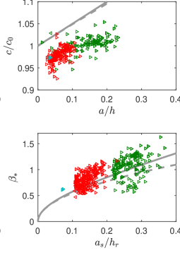
It should be emphasized that most waves propagate more slowly than $c_{0}$. Once the gas is formed, due to mass conservation, the solitons propagate on a reference level $h_{r}<h$. Osborne and Bergamasco (1986) show that solitons emerging from a sinusoidal forcing should propagate at

$$c=c_{0}\left(1+\frac{a_{s}+3(h_{r}-h)}{2h}\right)\,.$$ (12)

This can be also viewed as the solitons propagating against an adverse mean flow related to the trough of the initial sinusoidal wave. In Figure 13, the right-going soliton fit gives $a/h\simeq 0.2$ and $h_{r}/h\simeq 0.9$ so that $a_{s}/h=(a+h-h_{r})/h\simeq 0.3$ and $c\simeq c_{0}$ from (12). This is in good agreement with wave crest speeds detected by the Radon transform shown in Figure 14(c).

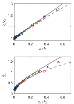
The sech² fit dimensionless shape parameter $\beta_{*}$ is plotted against its dimensionless soliton amplitude in Figure 14(d). It overall follows the trend predicted by non-linear theories but with a fair amount of scattering. This is due to both strong and weak interactions. Detected isolated pulses are generally narrower than KdV solitons. This is probably due to the high probability for a soliton to collide with another soliton in a weak interaction, which roughly takes place every 1 m (Figure 12a).

As a last remark, doubling the forcing amplitude from 6 mm to 12 mm leads to similar scaled soliton gas characteristics. In both cases the continuous forcing provides the energy input that compensates for viscous dissipation necessary to reach a statistically quasi-steady state. Reducing the forcing amplitude to 4 mm leads to a completely different steady standing wave regime. The thresholds for soliton gas occurrence might be worth further investigations.

5 Conclusions

A video system is shown to accurately measure waves propagating in both directions in a constant depth flume with full reflection at both ends. From a video camera pixel resolution of 1 mm, sub-pixel interface detection leads to an accuracy in water elevation likely better than one tenth of a millimeter when measuring waves several centimeters high. Crest wave speed is quantified with uncertainty of a few mm/s for waves propagating at about 1 m/s. This is done by applying the Radon transform on the $(x,t)$ field with a relatively high resolution, 1 cm $\times$ 0.025 s providing a good compromise between accuracy and computing time.

The monochromatic forcing at one end of the flume produces wave trains that can degenerate into a disorganized state identified as a soliton gas. The solitons, emerging from the periodic wave trains through non-linear steepening, experience multiple interactions that induce various phase shifts. Due to the many weak interactions (head-on collisions), the solitons detected in the gas are generally more peaky than KdV solitons. They are shown to propagate onto a reference level $h_{r}$ located below the mean water level $h$, as a consequence of mass conservation. Their speed is consequently smaller than that of KdV solitons propagating at constant depth $h$.

Redor et al. (2019) showed that both weak and strong interactions of two solitons can be properly described with the Kaup-Boussinesq (Kaup-Broer) integrable system of equations. Nabelek and Zakharov (2020) further suggest that soliton gases with many counter propagating solitons could be favorably analyzed with a dressing method for such set of equations, a promising track for future research. Since the final states in some of our experiments are highly nonlinear with solitons dominating the dynamics, the periodic Inverse Scattering Transform for the KdV equation (Osborne, 2010) could also be another approach to determining the number of emerging solitons and their amplitude (Redor, 2019).

References

- Almar et al. (2014) Almar R, Michallet H, Cienfuegos R, Bonneton P, Tissier M, Ruessink G (2014) On the use of the Radon Transform in studying nearshore wave dynamics. Coast Eng 92:24–30
- Aubourg and Mordant (2016) Aubourg Q, Mordant N (2016) Investigation of resonances in gravity-capillary wave turbulence. Phys Rev Fluids 1:023701
- Bonmarin et al. (1989) Bonmarin P, Rochefort R, Bourguel M (1989) Surface wave profile measurement by image analysis. Exp Fluids 7(1):17–24
- Carbone et al. (2016) Carbone F, Dutykh D, El GA (2016) Macroscopic dynamics of incoherent soliton ensembles: Soliton gas kinetics and direct numerical modelling. EPL (Europhys Lett) 113(3):30003
- Chen and Yeh (2014) Chen Y, Yeh H (2014) Laboratory experiments on counter-propagating collisions of solitary waves. Part 1. Wave interactions. J Fluid Mech 749:577–596
- Chen et al. (2014) Chen Y, Zhang E, Yeh H (2014) Laboratory experiments on counter-propagating collisions of solitary waves. Part 2. Flow field. J Fluid Mech 755:463–484
- Chou et al. (2004) Chou C, Yim J, Huang W (2004) Determining the hydrographic parameters of the surface of water from the image sequences of a ccd camera. Exp Fluids 36(4):515–527
- Cobelli et al. (2009) Cobelli PJ, Maurel A, Pagneux V, Petitjeans P (2009) Global measurement of water waves by fourier transform profilometry. Exp Fluids 46(6):1037
- Costa et al. (2014) Costa A, Osborne AR, Resio DT, Alessio S, Chrivì E, Saggese E, Bellomo K, Long CE (2014) Soliton Turbulence in Shallow Water Ocean Surface Waves. Phys Rev Lett 113(10):108501
- Deans (2007) Deans SR (2007) The Radon transform and some of its applications. Courier Corporation
- Ezersky et al. (2009) Ezersky A, Slunyaev A, Mouazé D, Chokchai W (2009) Occurrence of standing surface gravity waves modulation in shallow water. Eur J Mech-B/Fluids 28:521–531
- Guizien and Barthélemy (2002) Guizien K, Barthélemy E (2002) Accuracy of solitary wave generation by a piston wave maker. J Hydraul Res 40(3):321–331
- Hammack and Segur (1974) Hammack JL, Segur H (1974) The Korteweg-de Vries equation and water waves. Part 2. Comparison with experiments. J Fluid Mech 65(2):289–314
- Hasselmann (1962) Hasselmann K (1962) On the non-linear energy transfer in a gravity-wave spectrum. Part 1. General theory. J Fluid Mech 12(4):481–500
- Keulegan (1948) Keulegan GH (1948) Gradual damping of solitary waves. J Res Natl Bur Stand 40(6):487–498
- Kolaas et al. (2018) Kolaas J, Riise BH, Sveen K, Jensen A (2018) Bichromatic synthetic Schlieren applied to surface wave measurements. Exp Fluids 59(8):128
- Korteweg and de Vries (1895) Korteweg DJ, de Vries G (1895) On the change of form of long waves advancing in a rectangular channel, and on a new type of long stationary waves. Philos Mag 39(5):422–443
- Moisy et al. (2009) Moisy F, Rabaud M, Salsac K (2009) A synthetic Schlieren method for the measurement of the topography of a liquid interface. Exp Fluids 46(6):1021
- Nabelek and Zakharov (2020) Nabelek PV, Zakharov VE (2020) Solutions to the Kaup–Broer system and its (2+1) dimensional integrable generalization via the dressing method. Phys D: Nonlinear Phenom 409:132478
- Nazarenko (2011) Nazarenko S (2011) Wave turbulence, Lecture Notes in Physics, vol 825. Springer
- Osborne (2010) Osborne AR (2010) Nonlinear Ocean Waves and the Inverse Scattering Transform, International Geophysics Series, vol 97. Academic Press
- Osborne and Bergamasco (1986) Osborne AR, Bergamasco L (1986) The solitons of Zabusky and Kruskal revisited: Perspective in terms of the periodic spectral transform. Phys D: Nonlinear Phenom 18(1-3):26–46
- Pelinovsky and Sergeeva (2006) Pelinovsky E, Sergeeva A (2006) Numerical modeling of the KdV random wave field. Eur J Mech B-Fluids 25(4):425–434
- Redor (2019) Redor I (2019) Étude expérimentale de la turbulence intégrable en eau peu profonde. PhD thesis, Univ. Grenoble Alpes
- Redor et al. (2019) Redor I, Bartélemy E, Michallet H, Onorato M, Mordant N (2019) Experimental evidence of a hydrodynamic soliton gas. Phys Rev Lett 122:214502
- Renouard et al. (1985) Renouard D, Seabra-Santos F, Temperville A (1985) Experimental study of the generation, damping, and reflexion of a solitary wave. Dyn Atmos Oceans 9:341–358
- Sanchis and Jensen (2011) Sanchis A, Jensen A (2011) Dynamic masking of PIV images using the Radon transform in free surface flows. Exp Fluids 51:871–880
- Scott-Russell (1844) Scott-Russell J (1844) Report on waves. In: Proc. Roy. Soc. Edinburgh, vol 319
- Seabra-Santos et al. (1987) Seabra-Santos F, Renouard D, Temperville A (1987) Numerical and experimental study of the transformation of a solitary wave over a shelf or isolated obstacle. J Fluid Mech 176:117–134
- Taklo et al. (2017) Taklo TMA, Trulsen K, Krogstad HE, Borge JCN (2017) On dispersion of directional surface gravity waves. J Fluid Mech 812:681–697
- Trillo et al. (2016) Trillo S, Deng G, Biondini G, Klein M, Clauss GF, Chabchoub A, Onorato M (2016) Experimental observation and theoretical description of multisoliton fission in shallow water. Phys Rev Lett 117(14):144102
- Tsai (1987) Tsai R (1987) A versatile camera calibration technique for high-accuracy 3D machine vision metrology using off-the-shelf TV cameras and lenses. IEEE J Robotics Automation 3(4):323–344
- Umeyama (2017) Umeyama M (2017) Experimental study of head-on and rear-end collisions of two unequal solitary waves. Ocean Eng 137:174–192
- Zabusky and Galvin (1971) Zabusky NJ, Galvin CJ (1971) Shallow-water waves, the Korteweg-de Vries equation and solitons. J Fluid Mech 47(4):811–824
- Zakharov (1971) Zakharov VE (1971) Kinetic equation for solitons. Sov Phys JETP 33(3):538–540
- Zakharov (2009) Zakharov VE (2009) Turbulence in integrable systems. Stud Appl Math 122(3):219–234
- Zhang and Cox (1994) Zhang X, Cox C (1994) Measuring the two-dimensional structure of a wavy water surface optically: A surface gradient detector. Exp Fluids 17(4):225–237