MCMC-Interactive Variational Inference

Abstract

Leveraging well-established MCMC strategies, we propose MCMC-interactive variational inference (MIVI) to not only estimate the posterior in a time constrained manner, but also facilitate the design of MCMC transitions. Constructing a variational distribution followed by a short Markov chain that has parameters to learn, MIVI takes advantage of the complementary properties of variational inference and MCMC to encourage mutual improvement. On one hand, with the variational distribution locating high posterior density regions, the Markov chain is optimized within the variational inference framework to efficiently target the posterior despite a small number of transitions. On the other hand, the optimized Markov chain with considerable flexibility guides the variational distribution towards the posterior and alleviates its underestimation of uncertainty. Furthermore, we prove the optimized Markov chain in MIVI admits extrapolation, which means its marginal distribution gets closer to the true posterior as the chain grows. Therefore, the Markov chain can be used separately as an efficient MCMC scheme. Experiments show that MIVI not only accurately and efficiently approximates the posteriors but also facilitates designs of stochastic gradient MCMC and Gibbs sampling transitions.

Keywords: Gibbs sampling, stochastic gradient Langevin dynamics, designs of MCMC, Bayesian bridge regression, variational autoencoders

1 Introduction

Markov chain Monte Carlo (MCMC) has become a reference method for Bayesian inference, especially for tasks requiring high-quality uncertainty estimation. However, its applications to modern machine learning problems are challenged by complex models and big data. A primary reason is that MCMC is often restricted to reversible ergodic chains, like Metropolis-Hastings (MH) (Metropolis et al., 1953; Hastings, 1970) and Gibbs sampling (Geman & Geman, 1984), which require evaluating the likelihood over the whole data set. A number of MCMC schemes escaping reversibility with theoretical and/or empirical supports (Bierkens et al., 2019; Chen & Hwang, 2013; Neal, 1998) bring about considerable advantages such as accelerated mixing and enhanced adaptability to non-conjugate models, but their designs often demand significant efforts to achieve both efficacy and efficiency.

Stochastic gradient MCMCs (SG-MCMCs) (Welling & Teh, 2011; Ding et al., 2014; Ma et al., 2015; Li et al., 2016), which exploit the gradient information and neglect MH rejection steps, have been widely adopted for big data applications. Starting from arbitrary initial samples, SG-MCMCs move towards the stationary distribution via a random walk with step sizes annealed to zero. Thus it may either need labor-intensive tuning of the step-size annealing schedule, or easily suffer from slow mixing or high approximation errors. Variational inference (VI) approximates posterior $p(\bm{z}\,|\,\bm{x})$ with variational distribution ${\textstyle q(\bm{z})}$ by minimizing KL${\textstyle\left(q(\bm{z})\,||\,p(\bm{z}\,|\,\bm{x})\right)}$, the Kullback–Leibler (KL) divergence from $p(\bm{z}\,|\,\bm{x})$ to ${\textstyle q(\bm{z})}$ (Jordan et al., 1999; Blei et al., 2017). Though ${\textstyle q(\bm{z})}$ may underestimate uncertainty if its presumed distribution family ($e.g.$, diagonal Gaussian) is not flexible enough, VI is often much faster in finding a high posterior density region than MCMC which explores the whole parameter space by random jumps based on local information (Robert et al., 2018).

Inspired by the advantages of MCMC and VI that overcome each other’s limitations, we start a Markov chain with initial values drawn from an optimized variational distribution $q(\bm{z})$ so that the convergence can be expedited. If marginal distributions of this $q(\bm{z})$-mixed Markov chain are more flexible than the variational distribution family of $q$, there emerge interesting research questions: Can the framework of VI curb such a Markov chain from running wild as well as drive it towards the posterior? If yes, how can we design such a Markov chain that is (richly) parameterized and jointly optimized with $q(\bm{z})$ to deliver posterior approximations as good as valid MCMCs? Therefore, we are motivated to propose MCMC-interactive variational inference (MIVI) for efficient and high-quality uncertainty estimation. MIVI admits stochastic-gradient optimizations with a small number of MCMC updates of $q(\bm{z})$ and allows fast posterior sampling without keeping track of MCMC iterations. Furthermore, leveraging MCMCs that converge to the true posterior, we provide the parameterized Markov chain with an appropriate but adequate amount of flexibility to ease its optimization.

We encounter two-way difficulties when MCMC interacts with VI for mutual improvement. First, given an MCMC scheme, it is nontrivial to minimize the KL divergence from the posterior to the marginal distribution of the chain, because the density of the latter is often implicitly-defined by MCMC transitions. Second, even if the KL divergence is computable, it can be arduous to design a Markov chain that moderately improves $q$ without worrying about mode collapse or overdispersion. Our proposed MIVI has well addressed these challenges. To avoid calculating the KL divergence, we use a discriminator to estimate a log density ratio (Mescheder et al., 2017). To design a Markov chain that effectively improves $q$, MIVI borrows the idea of MCMC and (semi-)implicit VIs (Ranganath et al., 2016; Tran et al., 2017; Yin & Zhou, 2018; Molchanov et al., 2019; Titsias & Ruiz, 2018) and strikes a balance between flexibility and convergence to the true posterior. Concretely, we replace unfavorable components of a valid MCMC scheme by (richly) parameterized functions that is to be learned in the VI framework; we learn step sizes of a SG-MCMC for general-purpose inference and design model-specific Gibbs-sampling-like Markov chains for more accurate estimations at lower computing cost. More importantly, the optimized chain in MIVI can used separately as a valid MCMC. To the best our knowledge, MIVI is the first VI algorithm to utilize Gibbs sampling transitions and to facilitate their potential inspirition-driven designs.

2 Method description

MIVI is constructed by a variational distribution ${\textstyle q_{\phi}}$ mixed with a Markov chain, where ${\textstyle q_{\phi}}$ parameterized by $\phi$ is used to initialize $T\in\mathbb{Z}_{+}$ transitions of the chain. We use the marginal distribution of the chain at time $T$ as a refined variational distribution, written as ${\textstyle\tilde{q}^{(T)}_{\eta,\phi}(\bm{z})=\int h^{(T)}_{\eta}(\bm{z}\,|\,\bm{z}_{0})q_{\phi}(\bm{z}_{0})d\bm{z}_{0}}$ where ${\textstyle h^{(T)}_{\eta}}$ parameterized by ${\textstyle\eta}$ is the kernel of $T$ transitions of the chain. We show how to optimize $\phi$ and ${\textstyle\eta}$ in the framework of VI given valid formulations of ${\textstyle h^{(t)}_{\eta}}$, as well as how to formulate such ${\textstyle h^{(t)}_{\eta}}$ for monotonically non-increasing ${\textstyle\mbox{KL}(\tilde{q}^{(t)}_{\eta,\phi}(\bm{z})\,||\,p(\bm{z}\,|\,\bm{x}))}$ as ${\textstyle t}$ grows. With theoretical support provided, the short Markov chain admits extrapolation and fast posterior simulation. We defer all the proofs to Appendix. When there is no ambiguity, we omit the superscript $(T)$ and denote for brevity the marginal distribution by ${\textstyle\tilde{q}_{\eta,\phi}}$ and the transition by ${\textstyle h_{\eta}}$.

We first focus on optimizing $\phi$ and $\eta$ given a valid $h_{\eta}$. Suppose $p_{\theta}(\bm{x},\bm{z})=p_{\theta}(\bm{x}\,|\,\bm{z})p(\bm{z})$ is the joint likelihood of data $\bm{x}$ given $\bm{z}$ and prior $p(\bm{z})$. We optimize $\theta$, $\phi$, and $\eta$ to maximize the ELBO:

$${\textstyle\max\limits_{\theta,\phi,\eta}\mathbb{E}_{\tilde{q}_{\eta,\phi}(\bm{z})}\log\frac{p_{\theta}(\bm{x},\bm{z})}{\tilde{q}_{\eta,\phi}(\bm{z})}=\max\limits_{\theta,\phi,\eta}\mathbb{E}_{\tilde{q}_{\eta,\phi}(\bm{z})}\log\frac{p_{\theta}(\bm{x},\bm{z})}{q_{\phi}(\bm{z})}-\mbox{KL}(\tilde{q}_{\eta,\phi}(\bm{z})\,||\,q_{\phi}(\bm{z})).}$$ (1)

The first term on the right-hand side of (1) is simple to estimate if the transition $h_{\eta}$ is reparameterizable. Difficulty lies in $\mbox{KL}(\tilde{q}_{\eta,\phi}(\bm{z})\,||\,q_{\phi}(\bm{z}))$ because marginal distribution $\tilde{q}_{\eta,\phi}(\bm{z})$ is not always in closed form. To circumvent the difficulty we use a discriminator to estimate $\log\frac{\tilde{q}_{\eta,\phi}(\bm{z})}{q_{\phi}(\bm{z})}$ which only requires to draw random samples from the two distributions (Mescheder et al., 2017). Specifically, with fixed $\tilde{q}_{\eta,\phi}(\bm{z})$ and $q_{\phi}(\bm{z})$, an optimal discriminator that is able to distinguish samples from the two distributions will be $D^{*}(\bm{z})=\log\tilde{q}_{\eta,\phi}(\bm{z})-\log q_{\phi}(\bm{z})$ that solves

$${\textstyle\max\nolimits_{D}\mathbb{E}_{\tilde{q}_{\eta,\phi}(\bm{z})}\log\sigma(D(\bm{z}))+\mathbb{E}_{q_{\phi}(\bm{z})}\log(1-\sigma(D(\bm{z}))),}$$ (2)

where $\sigma(\cdot)$ is the sigmoid function. Consequently, (1) turns out to be

$${\textstyle\max\nolimits_{\theta,\phi,\eta}\mathbb{E}_{\tilde{q}_{\eta,\phi}(\bm{z})}\left[\log{p_{\theta}(\bm{x},\bm{z})}-\log{q_{\phi}(\bm{z})}-D^{*}(\bm{z})\right].}$$ (3)

2.1 Optimization

Theoretically, the ELBO (3) can be maximized if the discriminator is flexible enough. In practice, however, the saturation of the sigmoid function in the cross-entropy loss of (2) undermines the power of $D$ to distinguish samples from $q_{\phi}$ and $\tilde{q}_{\eta,\phi}$. Concretely, if $q_{\phi}$ is far from $\tilde{q}_{\eta,\phi}$, the optimization procedure encourages large $D$, driving $\sigma(D)$ to approach value $1$ which is a saturation region of the sigmoid function, and consequently, the diminished gradient significantly slows down $D$ from getting bigger. Meanwhile, when maximizing the ELBO of (3) with an under-optimized discriminator $D$ for $\mbox{KL}(\tilde{q}_{\eta,\phi}(\bm{z})\,||\,q_{\phi}(\bm{z}))$, a small increase of $D$ cannot compensate for a much larger increase of the cross entropy $-\mathbb{E}_{\tilde{q}_{\eta,\phi}}\log{q_{\phi}(\bm{z})}$ if $q_{\phi}$ and $\tilde{q}_{\eta,\phi}$ are too far from each other. In short, a big discrepancy between $q_{\phi}$ and $\tilde{q}_{\eta,\phi}$ impedes optimizing the discriminator and a poor discriminator further spaces the two distributions. This vicious circle often makes (3) fail to increase $\mathbb{E}_{\tilde{q}_{\eta,\phi}(\bm{z})}\log{p_{\theta}(\bm{x},\bm{z})}$ and hence brings about poor estimations of $\tilde{q}_{\eta,\phi}$ and $q_{\phi}$ that drift apart from each other.

Even if the discriminator is so flexible that it is unaffected by the vicious circle, optimizing (3) by gradient ascent with respect to $\phi$ can be intractable because $D^{*}$ itself, found by (2), depends on $\phi$. The problem of calculating this gradient cannot be solved by the strategy of Mescheder et al. (2017) after the Markov chain is introduced. To circumvent the two aforementioned difficulties when using the discriminator, MIVI reformulates the objective by maximizing a lower bound of (3) with respect to $\theta$ and $\eta$ given optimal $D^{*}$ and $\phi^{*}$ that are obtained by two auxiliary optimization problems. This lower bound and the two auxiliary optimization problems are expressed as

$$\max\nolimits_{\theta,\eta}\mathbb{E}_{\tilde{q}_{\eta,\phi^{*}}(\bm{z})}\left[\log{p_{\theta}(\bm{x},\bm{z})}-\log{q_{\phi^{*}}(\bm{z})}-D^{*}(\bm{z})\right],$$ (4)

$$D^{*}=\arg\max\nolimits_{D}\mathbb{E}_{\tilde{q}_{\eta,\phi^{*}}(\bm{z})}\log\sigma(D(\bm{z}))+\mathbb{E}_{q_{\phi^{*}}(\bm{z})}\log(1-\sigma(D(\bm{z}))),$$ (5)

$$\phi^{*}=\arg\min\nolimits_{\phi}-\mathbb{E}_{\tilde{q}_{\eta,\phi}(\bm{z})}\log{q_{\phi}(\bm{z})}.$$ (6)

It is straightforward to take the gradient of (4) and (6) with respect to $\theta$ and $\phi$, respectively. More importantly, the following property overcomes the difficulty in taking the gradient of $D^{*}$ with respect to $\eta$ when maximizing (4) under the assumption of reparameterizable Markov chain transitions.

Property 1.

Suppose $h_{\eta}$ is reparameterizable, which means there exists a deterministic vector-valued function ${\textstyle f_{\eta}}$ and a random vector $\varepsilon$ such that ${\textstyle\bm{z}^{(T)}\sim\tilde{q}_{\eta,\phi}}$ is equivalent to ${\textstyle\bm{z}^{(T)}=f_{\eta}(\bm{z}^{(0)},\varepsilon)}$ where ${\textstyle\bm{z}^{(0)}\sim q_{\phi}(\bm{z})}$. The gradient of (4) with respect to ${\textstyle\eta}$ is equal to

2.2 Formulation of Markov chain transitions

We have discussed the optimization of $\theta$, $\phi$ and $\eta$ in MIVI. But MIVI makes sense only if $\tilde{q}_{\eta,\phi}$ is a better posterior approximation than $q_{\phi}$. Yet to be determined is the formulation of a valid transition $h_{\eta}$ that keeps pushing $\tilde{q}_{\eta,\phi}(\bm{z})$ closer to $p(\bm{z}\,|\,\bm{x})$ and thus enables extrapolation of the short Markov chain. We utilize stochastic gradient Langevin dynamics (SGLD) (Welling & Teh, 2011) as a general-purpose solution and Gibbs sampling for model-specific but more efficient inference.

SGLD     So far $h_{\eta}$ being reparameterizable is the only assumption of MIVI on the Markov chain. Consequently, SGLD can be incorporated in MIVI and universally applied, as it approximates posteriors with stochastic gradient descent and injected Gaussian noise. Concretely, for a mini batch $x$ of size $n$ from training data of size $N$, a variable $z$ at discrete time $t$ of SGLD is updated by

$${\textstyle z^{(t)}=z^{(t-1)}+\frac{\eta_{t}}{2}[\nabla_{z}\log p(z^{(t-1)})+\frac{N}{n}\nabla_{z}\log p(x\,|\,z^{(t-1)})]+\epsilon_{t},~{}~{}~{}\epsilon_{t}\sim\mathcal{N}(0,\eta_{t})}$$ (7)

where $\eta_{t}$ is the step size at time $t$. With a long run and diminishing $\eta_{t}$, SGLD proceeds through two phases (Welling & Teh, 2011): the first is the phase of stochastic optimization in which $p(\bm{x},\bm{z})$ is being maximized, and the second is the phase of Langevin dynamics in which a random walk is approximating the posterior sampling. With standard assumptions (Khasminskii, 2011; Vollmer et al., 2016) to guarantee ergodicity and diminishing step sizes, SGLD converges to a stationary distribution that well approximates the true posterior. Particularly, Teh et al. (2016) provide conditions under which SGLD converges to the posterior and find consistent posterior estimators with asymptotic normality. The following lemma validates the use of any $T$ steps of SGLD transitions in MIVI and an extrapolation ($i.e.,$ more than $T$ steps of transitions).

Lemma 1 (Page 81 of Cover & Thomas (2006)).

Suppose $\bm{z}$ are variables on a Markov chain $M$ with the stationary distribution $\pi(\bm{z})$. Let $\mu^{(t)}$ be any distribution on the state space of $M$ at $t$ and $\mu^{(t+1)}$ be the marginal distribution after one transition from $\mu^{(t)}$. Let $q$ denote the mass/density function of variables $\bm{z}^{(t)}\sim\mu^{(t)}$ or $\bm{z}^{(t+1)}\sim\mu^{(t+1)}$. We have ${\textstyle\emph{\mbox{KL}}(q(\bm{z}^{(t)})\,||\,\pi(\bm{z}))\geq\emph{\mbox{KL}}(q(\bm{z}^{(t+1)})\,||\,\pi(\bm{z})).}$

Specifically, Lemma 1 sheds light on SGLD’s continuously refined $\tilde{q}_{\eta,\phi}^{(t)}$ in terms of its KL divergence from the stationary distribution, for not only $t\leq T$ in MIVI, but also $t>T$ in extrapolation as long as the step sizes appropriately anneal. The guaranteed superiority of $\tilde{q}_{\eta,\phi}^{(t)}$ over $q_{\phi}$, however, is not enough; running a finite number of transitions, people also seek a balance of fast convergence (low variance) and small discretization errors (low bias) by a good selection of step sizes which may need to be tuned labor-intensively. To this end, MIVI incorporates $T$ transitions of SGLD, sets $\eta$ of $h_{\eta}$ as step sizes $\{\eta_{1},\ldots,\eta_{T}\}$, and optimizes $\eta$ by (4) for a good bias-variance tradeoff. Moreover, with $q_{\phi}$ of MIVI locating high posterior density regions, the $T$ transitions start from the second phase of SGLD and the optimized step sizes can be leveraged to extrapolate the markov chain to any length $t$, $T<t<\infty$ for even better posterior estimations.

Gibbs sampling    In addition to SGLD, Lemmas 2 and 3 show MIVI can utilize reparameterizable Gibbs sampling transitions to keep improving ${\textstyle\tilde{q}^{(t)}_{\eta,\phi}(\bm{z})}$ as ${\textstyle t}$ increases and, more significantly, facilitate an efficient design of MCMC alternative to Gibbs sampling. Specifically, it is implied that for a Markov chain of variables ${\textstyle\bm{z}}$ of interest and (auxiliary) variables ${\textstyle\bm{w}}$, using a valid Gibbs sampling transition for ${\textstyle\bm{z}}$ will keep pushing its marginal distribution closer to the posterior as long as the Markov chain’s transition for ${\textstyle\bm{w}}$ is good enough.

Lemma 2.

Suppose the transition of a Markov chain $M$ of $(\bm{w},\bm{z})$ at time $t+1$ is $r$ such that $r(\bm{w}^{(t+1)},\bm{z}^{(t+1)}\,|\,\bm{w}^{(t)},\bm{z}^{(t)})=r(\bm{z}^{(t+1)}\,|\,\bm{w}^{(t)})r(\bm{w}^{(t+1)}\,|\,\bm{z}^{(t+1)})$. Let $\mu^{(t)}$ be any distribution on the state space of $M$ at $t$ and $\mu^{(t+1)}$ be the marginal distribution after one transition from $\mu^{(t)}$. Let $q$ denote the joint mass/density function and thus $\textstyle q(\bm{w}^{(t)},\bm{z}^{(t)},\bm{w}^{(t+1)},\bm{z}^{(t+1)})=q(\bm{w}^{(t)},\bm{z}^{(t)})r(\bm{w}^{(t+1)},\bm{z}^{(t+1)}\,|\,\bm{w}^{(t)},\bm{z}^{(t)}).$ If $r(\bm{z}\,|\,\bm{w})$ is the conditional distribution of $\bm{z}$ given $\bm{w}$ and hence a valid transition of $\bm{z}$ in a Gibbs sampler $G$ that converges to the posterior $\pi(\bm{w},\bm{z})$, then ${\textstyle\mbox{KL}(q(\bm{w}^{(t)},\bm{z}^{(t)})\,||\,\pi(\bm{w},\bm{z}))\geq\mbox{KL}(q(\bm{w}^{(t)},\bm{z}^{(t+1)})\,||\,\pi(\bm{w},\bm{z})).}$

Lemma 3.

With all the assumptions in Lemma 2, suppose $\mu^{\prime(t)}$ is the posterior with density $\pi(\bm{w},\bm{z})$ and is at time $t$ of $M$. $q^{\prime}$ denotes the joint mass/density of variables from $\mu^{\prime(t)}$ and $\mu^{\prime(t+1)}$. If $r(\bm{w}\,|\,\bm{z})$ at time $t$ is close to $\pi(\bm{w}|\bm{z})$ in the sense that $\mathbb{E}_{q(\bm{z}^{(t)})}\left[\mbox{KL}(r(\bm{w}\,|\,\bm{z}^{(t)})\,||\,\pi(\bm{w}\,|\,\bm{z}^{(t)}))\right]\leq\mathbb{E}_{q(\bm{z}^{(t+1)})}\left[\mbox{KL}(q(\bm{w}^{(t)}\,|\,\bm{z}^{(t+1)})\,||\,q^{\prime}(\bm{w}^{(t)}\,|\,\bm{z}^{(t+1)}))\right]$, then ${\textstyle\mbox{KL}(q(\bm{z}^{(t)})\,||\,\pi(\bm{z}))\geq\mbox{KL}(q(\bm{z}^{(t+1)})\,||\,\pi(\bm{z})).}$

As shown by Lemma 2 and 3, if $(\bm{w},\bm{z})$ are variables of interest and the full conditional distribution $p(\bm{z}\,|\,\bm{w},\bm{x})$ is reparameterizable, we can use $p(\bm{z}\,|\,\bm{w},\bm{x})$ as the transition of $\bm{z}$ in the Markov chain. Furthermore, a (richly) parameterized transition function $h^{(1)}_{\eta}(\bm{w}\,|\,\bm{z},\bm{x})$ is learned by MIVI to well approximate the full conditional distribution $p(\bm{w}\,|\,\bm{z},\bm{x})$ so that, by Lemma 3, $\bm{z}^{(t)}$ approaches to the true posterior $p(\bm{z}\,|\,\bm{x})$ as $t$ increases, not only within the $T$ transitions of MIVI, but also for $t>T$ when the extrapolated chain serves as an MCMC scheme. This is especially useful when we care about posterior estimates of $\bm{z}$ more than $\bm{w}$. Moreover, iterating $p(\bm{w}\,|\,\bm{z},\bm{x})$ and $h^{(1)}_{\eta}(\bm{w}\,|\,\bm{z},\bm{x})$ is an efficient MCMC scheme with fast mixing because the optimized $h^{(1)}_{\eta}(\bm{w}\,|\,\bm{z},\bm{x})$ by MIVI has located high density regions of $p(\bm{w}\,|\,\bm{z},\bm{x})$. We provide in Section 4 specific applications where $\bm{w}$ are auxiliary variables enabling a closed-form reparameterizable full conditional distribution of $\bm{z}$.

2.3 MIVI implementation

Instead of keeping the discriminator $D$ and ${\phi}$ optimal in every epoch when optimizing $\theta$ and $\eta$, we regard the problem as a three-player game analogous to the two-player game of Mescheder et al. (2017) in order to reduce the computing cost: 1) Given $D$ and $\phi$, we optimize $\eta$ and $\theta$ to maximize ELBO (4). 2) Given $\eta$, we optimize $\phi$ to reduce the discrepancy between $q_{\phi}$ and $\tilde{q}_{\eta,\phi}$ measured by the cross entropy (6). 3) The discriminator $D$ tries to differentiate samples from $\tilde{q}_{\eta,\phi}$ and $q_{\phi}$. Note that $\eta$ and $\phi$ are learned adversarially and the game terminates at a saddle point that is a maximum of (4) with respect to $\eta$’s strategy and a minimum of (6) with respect to $\phi$’s strategy. The ELBO of MIVI, $\mathbb{E}_{\tilde{q}_{\eta,\phi}(\bm{z})}\log\frac{p_{\theta}(\bm{x},\bm{z})}{\tilde{q}_{\eta,\phi}(\bm{z})}$, is bounded above as in Property 2.

Property 2.

${\textstyle\mathbb{E}_{\tilde{q}_{\eta,\phi}(\bm{z})}\log\frac{p_{\theta}(\bm{x},\bm{z})}{\tilde{q}_{\eta,\phi}(\bm{z})}\leq\mathbb{E}_{\tilde{q}_{\eta,\phi}(\bm{z})}\log\frac{p_{\theta}(\bm{x},\bm{z})}{q_{\phi}(\bm{z})}}.$

The upper bound together with saturation of $\sigma(D)$ provides a fast pre-training strategy. Concretely, given $\phi^{*}$ and $D^{*}$ we assume $\sigma(D^{*})$ saturates such that $\mathbb{E}_{\tilde{q}_{\eta,\phi^{*}}(\bm{z})}D^{*}(\bm{z})\leq c$ for some positive constant $c$ (that may depend on $\eta$ and $\phi^{*}$). Consequently, (4) is bounded between ${\textstyle(\mathbb{E}_{\tilde{q}_{\eta,\phi^{*}}(\bm{z})}\log\frac{p_{\theta}(\bm{x},\bm{z})}{q_{\phi^{*}}(\bm{z})}-c)}$ and ${\textstyle\mathbb{E}_{\tilde{q}_{\eta,\phi^{*}}(\bm{z})}\log\frac{p_{\theta}(\bm{x},\bm{z})}{q_{\phi^{*}}(\bm{z})}}$ which, instead, can be optimized to avoid potentially the most time-consuming training of $D$. We summarize the implementation of MIVI as Algorithm 1 in Appendix. We find that MIVI is numerically stable and converges fast as shown in Section 4.

3 Related work and contribution

Using a discriminator to approximate a hard-to-compute KL divergence was first introduced by Mescheder et al. (2017) that enable an arbitrarily flexible variational distribution. It is also adopted by Li et al. (2017) where the variational posterior is supervised by SG-MCMC. But in their training procedure the discriminator and variational parameters are entangled in a way that makes it difficult to rigorously calculate the gradient of the objective function. By contrast, we reformulate the objective with auxiliary optimization problems and provide rigorously derived gradients. Learning step sizes of SGLD by VI has been explored by Gallego & Insua (2019) and Nijkamp et al. (2020). The former utilizes the Gaussianity of SGLD transitions, and the latter regard SGLD as a normalizing flow that assumes a volume-preserving invertible transformation. Both methods depend on the good properties of SGLD. Comparatively, the reformulated optimizations of MIVI make it well adapted to different kinds of MCMCs with reparameterizable transitions, so that many SG-MCMCs, like Hamiltonian and Langevin dynamics, and Gibbs sampling schemes can be incorporated.

While VI and MCMC have complementary properties, existing works combining the two have primarily studied one-way improvement. As for utilizing MCMC to facilitate VI, a common practice is using the refined MCMC marginal distribution to guide and improve the variational distribution. Ruiz & Titsias (2019) minimize the discrepancy between the variational and a marginal distribution of Hamilton Monte Carlo (HMC) using the contrastive divergence without explicitly computing the KL divergence. Titsias (2017) implicitly augments the variational distribution by MCMC and a model-based reparameterization. Salimans et al. (2015) incorporate in VI finite steps of MCMC and the MCMC samples are inferred as auxiliary variables; HMC is adopted to illustrate this idea and is related to normalizing flow. Generally, Rezende & Mohamed (2015) write Hamiltonian and Langevin dynamics as infinitesimal flows; both flows can be used in VI for a tighter ELBO and the inference requires volume-preserving invertible transformations. Zhang et al. (2020) construct measure preserving flows and utilize distribution preservation of Hamilton Monte Carlo. Chen et al. (2017) propose the use of Langevin dynamics as a way to transit from one latent variable to the next to improve variational autoencoders (VAEs).

On the other hand, research of using VI to facilitate MCMC includes de Freitas et al. (2001) that use a variational distribution as the MH proposal to alleviate the poor scaling with dimension of the independent Metropolis algorithm. Habib & Barber (2019) learn a lower-dimensional embedding of the parameters of interest by VI to accelerate MCMC mixing. Several works share the idea of providing MCMC proposals with more flexibility by introducing auxiliary variables (Maddison et al., 2017; Naesseth et al., 2018; Le et al., 2018). In comparison, we fulfill mutual improvement of VI and MCMC by MIVI. Being a marginal distribution of valid MCMCs, the variational distribution of MIVI gets closer to the posterior. MIVI replaces unfavorable parts (like unknown, non-reparameterizable or manually tuned transitions, see Section 4) of MCMCs by (richly) parameterized functions and learns them in the framework of VI. In this way, MIVI facilitates designs of MCMCs. More importantly, with theoretical support, the chain in VI can be extrapolated and used as an efficient alternative to well established MCMCs. In addition, to the best of our knowledge, MIVI is the first method to combine VI and Gibbs sampling.

4 Experiments

We first use toy data (deferred to Appendix) and a negative binomial (NB) model to illustrate the flexibility of MIVI incorprating a few SGLD transitions. Next, we use both Bayesian logistic and bridge regression to show MIVI and Gibbs sampling facilitate each other when some of the Gibbs sampling transitions are unknown or not reparameterizable. In addition, we provide experiments of variational autoencoders (VAEs) (Kingma & Welling, 2014) by MIVI and demonstrate its remarkable performance compared to existing state-of-the-art algorithms. We use Adam (Kingma & Ba, 2014) to otpimize $\theta$, $\phi$, $\eta$ and $D$ with the learning rate as $0.001$. Throughout this section unless specified, the prior $p(\bm{z})$ used in Gibbs sampling, mean-field VI (MFVI), and MIVI is $\mathcal{N}(0,I)$ for real-valued $\bm{z}$ and the variational distribution $q_{\phi}(\bm{z})$ is a diagonal Gaussian whose mean and log of variances constitute $\phi$. We set $\eta$ as the step sizes of SGLD if incorporated in MIVI, and for simplicity, a time-invariant step size is set and learned. The learned step size can initialize an appropriate decay, like the one suggested by Teh et al. (2016). Also see Vollmer et al. (2016) for theoretical analysis of SGLD with a fixed step size. More experiment settings are deferred to Appendix.

4.1 Negative binomial model

We draw 1,000 random samples from negative binomial (NB) distribution $\mbox{NB}(x\,|\,r=2,p=0.7)$ whose probability $p(x)=\frac{\Gamma(x+r)}{\Gamma(r)x!}p^{x}(1-p)^{r}$ for $x\in{0}\cup\mathbb{Z_{+}}$. We use $r\sim\mbox{Gamma}(0.1,0.1)$ and $p\sim\mbox{Beta}(0.1,0.1)$ as the prior. Posteriors of $r$ and $p$ under the NB model are estimated by Gibbs sampling (Zhou et al., 2012), MFVI, and MIVI. We set $z=(\log(r),\mbox{logit}(p))$ in MFVI and MIVI that incorporates $T=10$ SGLD transitions. Shown in Figure 1 (a) are the estimated density contour plots of $(r,p)$ by Gibbs sampling and the one transformed from $(\log(r),\mbox{logit}(p))\sim q_{\phi}$ by MFVI. Analogously plotted in Figure 1 (b) are the densities of $(r,p)$ resulting from $q_{\phi}$ and $\tilde{q}_{\eta,\phi}$ by MIVI. The negative correlation in the posterior of $r$ and $p$ as shown by Gibbs sampling has been well recovered by $\tilde{q}_{\eta,\phi}$ in MIVI. Furthermore, the diagonal Gaussian $q_{\phi}$ in MFVI has underestimated the parameter uncertainty whereas $q_{\phi}$ of the same family in MIVI gives much better variance estimations because MIVI restrains the discrepancy between $q_{\phi}$ and $\tilde{q}_{\eta,\phi}$.

(a) NB: Gibbs and MFVI.

(b) NB: MIVI.

(c) Logistic: $\beta$.

(d) Logistic: $\omega$.

Figure 1: Estimated posterior densities. (a) and (b) are the estimated posteriors of $r$ and $p$ for the negative binomial model by Gibbs sampling (red), MFVI (gray) and MIVI (orange for $q_{\phi}$ and blue for $\tilde{q}_{\eta,\phi}$), respectively. (c) and (d) are the estimated posteriors of the logistic regression coefficient $\beta$ and the auxiliary Polya gamma random variable $\omega$ by Gibbs sampling (red) and $\tilde{q}_{\eta,\phi}$ of MIVI (blue).

Next, we accentuate MIVI that uses Gibbs sampling transitions for variables $\bm{z}$ and replaces unknown or non-reparameterizable Gibbs transitions for variables $\bm{w}$ by (richly) parameterized functions. Compared to SGLD, MIVI needs fewer Gibbs-sampling-like transitions without sacrificing capacity, and the inferred $\tilde{q}_{\eta,\phi}$ gives comparable posterior estimates to Gibbs sampling. Examples include Bayesian logistic and bridge regression using auxiliary variables that are difficult to find or sample.

4.2 Bayesian logistic regression

One of the most well-known data augmentation schemes is the Polya gamma (PG) augmentation for logistic regression (Polson et al., 2013), making the regression coefficients have Gaussian conditional distributions. Specifically, given a unique $\bm{x}_{i}$, $i=1,\cdots,n$, and $y_{i}\sim\mbox{Bernoulli}(\sigma(\bm{x}_{i}^{\prime}{\beta}))$, $p(y_{i}\,|\,x_{i},\beta)=\frac{e^{y_{i}\bm{x}_{i}^{\prime}\beta}}{1+e^{\bm{x}_{i}^{\prime}\beta}}=\frac{e^{(y_{i}-\frac{1}{2})\bm{x}_{i}^{\prime}\beta}}{2}\int_{0}^{\infty}e^{-\omega_{i}(\bm{x}_{i}^{\prime}\beta)^{2}/2}p(\omega_{i})d\omega_{i}$ where $p(\omega_{i})$ is the density of $\mbox{PG}(1,0)$ prior on $\omega_{i}$. The conditional posterior of $\omega_{i}$ is $\mbox{PG}(1,\bm{x}_{i}^{\prime}\beta)$ and that of $\beta$ is a Gaussian distribution. Iterating the samplings from both distributions defines a valid Gibbs sampler (see Appendix for details). However, PG distributions are not reparameterizable. Therefore, in the Markov chain of MIVI we use the Gaussian full conditional distribution as the transition for $\beta$ and a neural network $g_{\eta}$ parameterized by $\eta$ for local variables $\omega_{i}$’s. Specifically, concatenating $\bm{x}_{i}^{\prime}\beta$ and an independent Gaussian random vector $\epsilon_{i}$ as the input of $g_{\eta}$, the Markov chain in MIVI proceeds by iterating $\omega_{i}=g_{\eta}(\bm{x}_{i}^{\prime}\beta,\epsilon_{i})$ and $(\beta\,|\,-)\sim\mathcal{N}\left(\Sigma_{\beta}(X^{\prime}\kappa+I),\Sigma_{\beta}\right)$, where $\Sigma_{\beta}=(X^{\prime}\Omega X+I)^{-1}$, $\Omega=\mbox{diag}(\omega_{1},\ldots,\omega_{n})$, and $\kappa=(y_{1}-0.5,\cdots,y_{n}-0.5)$.

We synthesize a data set of 1,000 four-dimenstional, correlated $\bm{x}_{i}\sim\mathcal{N}(0,\Sigma)$ where the elements of $\Sigma$ are $\sigma_{v,v}=1$, $v=1,2,3,4$, $\sigma_{1,2}=\sigma_{2,1}=-0.8$, $\sigma_{3,4}=\sigma_{4,3}=0.9$ and other $\sigma_{v,v^{\prime}}=0$. True $\beta=(\beta_{1},\beta_{2},\beta_{3},\beta_{4})$ is set to be $(-2,-1,1,2)$ and $y_{i}\sim\mbox{Bernoulli}(\sigma(\bm{x}_{i}^{\prime}\beta))$. Good estimations of $\beta_{1}$ and $\beta_{2}$ should be positively correlated and $\beta_{3}$ and $\beta_{4}$ negatively correlated. We run only one transition of the Markov chain in MIVI (i.e., $T=1$) and compare $\tilde{q}_{\eta,\phi}$ with Gibbs sampling. Shown in Figure 1 (c) and (d), respectively, are the estimated posterior of $\beta$ and of $\omega$ averaged over data which is $\int p(\omega\,|\,\bm{x})p(\bm{x})d\bm{x}$. As a result, $\tilde{q}_{\eta,\phi}$ of MIVI gives rise to comparable posterior estimations to Gibbs sampling. We plot in Appendix the estimated posterior $\omega_{i}$ for some randomly selected $i$ which are also similar to those from Gibbs sampling. Additionally, logistic regression of binary MNIST (3 v.s. 5) by MIVI achieves a testing accuracy of $95.79\%$ that matches $95.64\%$ from the MLE of a well-tuned $L_{2}$-penalized logistic regression. Also provided in Appendix are estimated distributions of $\omega_{i}$ from $\tilde{q}_{\eta,\phi}$ associated to randomly selected MNIST training images. Therefore, having well approximated the non-reparameterizable Gibbs sampling transition of $\omega_{i}$’s by a neural network, MIVI delivers posterior estimations on par with Gibbs sampling and preserves the classification capacity.

4.3 Bayesian bridge regression

(a) $\alpha=1$ (Lasso).

(b) $\alpha=0.5$.

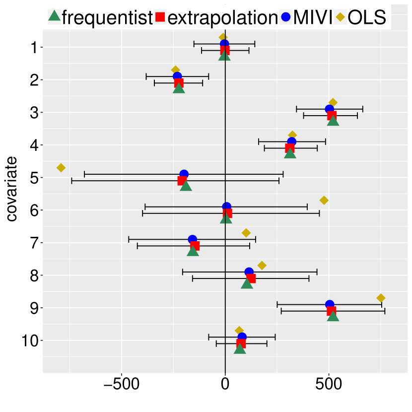
(c) $\alpha=1.5$.

Figure 2: Bridge regression of diabetes data. (a) is results of $\alpha=1$ (Lasso), (b) $\alpha=0.5$ and (c) $\alpha=1.5$, including point estimates of $\beta$ by a frequentist approach (green triangle) minimizing the loss function, Gibbs sampling or the extrapolated Markov chain (red square), $\tilde{q}_{\eta,\phi}$ of MIVI (blue dot) and OLS (yellow diamond) and the $95\%$ CIs by Gibbs (or the extrapolated chain) and MIVI.

Next we show MIVI not only well approximates posteriors but also helps to design valid Gibbs-sampling-like MCMC when some Gibbs sampler transitions are unknown in analytic expressions. Bridge regression tries to find $\hat{\beta}=(\hat{\beta}_{1},\ldots,\hat{\beta}_{p})$ that minimizes $\frac{1}{2}||y-X\beta||^{2}+\psi\sum_{v=1}^{p}|\beta_{v}|^{a}$ given the choice of $\alpha\in(0,2)$ and $\psi>0$. From a Bayesian perspective, a hirarchical model for bridge regression is $p(y\,|\,X,\beta,\sigma)=\mathcal{N}(y\,|\,X\beta,\sigma^{2}I)$, $p(1/\sigma^{2})=\mbox{Gamma}(1/\sigma^{2}\,|\,r,c)$, and $p(\beta_{v}\,|\,\alpha,\rho,\sigma)\propto e^{-\rho|\beta_{v}/\sigma|^{\alpha}}$ for $v=1,\ldots,p$, where $r$ and $c$ are the gamma shape and rate parameter, respectively, and $\rho$ is a hyper-parameter regularizing the $L_{\alpha}$ norm of $\beta$. A data augmentation that writes $p(\beta_{v}\,|\,\alpha,\rho,\sigma)$ as a scale mixture of normals enables conjugacy. Specifically, ${\textstyle e^{-\rho|\beta_{v}/\sigma|^{\alpha}}=\int_{0}^{\infty}e^{-\frac{\lambda_{v}\beta_{v}^{2}}{2\sigma^{2}}\rho^{2/\alpha}}g(\lambda_{v})d\lambda_{v}}$, where $g(\lambda_{v})$ is proportional to the density of a positive stable distribution with index of stability ${\alpha}/{2}$ (West, 1987; Polson et al., 2014). While both the prior and full conditional of $\beta$ are Gaussian, neither the posterior nor the full conditional distribution of $\lambda_{v}$ is known in closed form, which impedes an efficient Gibbs sampler under this data augmentation.

To circumvent the unknown conditional distribution of global variables $\lambda_{v}$’s, we use a flexible reparameterizable distribution to approximate their marginal distribution which serves as a time-invariant transition of $\lambda_{v}$’s in the Markov chain of MIVI. For simplicity, we adopt Weibull distributions as $\lambda_{v}\sim\mbox{Weibull}(a_{v},b_{v})$, which is equivalent to $\lambda_{v}=a_{v}e^{\log(-\log u)/b_{v}}$, $u\sim\mbox{Uniform}(0,1)$, but other flexible distributions on $\mathbb{R}_{+}$, like a neural network with random noise as input, also work as long as they are reparameterizable. Given $\lambda_{v}$’s, $\beta$ and $\sigma^{2}$ are updated according to their full conditional distributions. Concretely, the Markov chain of MIVI proceeds by iterating

$${\textstyle(\lambda_{v}\,|\,-)\sim\mbox{Weibull}(a_{v},b_{v}),~{}v=1,\ldots,p,~{}~{}~{}~{}~{}~{}(\beta\,|\,-)\sim\mathcal{N}(\Sigma X^{\prime}y,\sigma^{2}\Sigma),}$$

$$(1/\sigma^{2}\,|\,-)\sim\textstyle\mbox{Gamma}(r+\frac{n+p}{2},c+\frac{1}{2}||y-X\beta||^{2}+\frac{1}{2}\sum_{v=1}^{p}\rho^{2/\alpha}\lambda_{v}\beta_{v}^{2}),$$ (8)

where $\Sigma=(X^{\prime}X+\rho^{2/\alpha}\Lambda)^{-1}$, $\Lambda=\mbox{diag}(\lambda_{1},\cdots,\lambda_{p})$, and $n$ is the number of observations. With $\eta=(\log a_{1},\log b_{1},\ldots,\log a_{p},\log b_{p})$ optimized by MIVI, the Markov chain can be extrapolated to approximate a collapsed Gibbs sampler whose transition of $\lambda_{v}$’s are their marginal distributions. Note that bridge regression is reduced to Lasso if $\alpha=1$ and a Gibbs sampler is feasible by imposing a Laplacian prior on $\beta$ (Park & Casella, 2008). When $\alpha\neq 1$, Polson et al. (2014) has proposed a Gibbs sampler that requires truncated multivariate distributions for parameter updates, which may require inefficient rejection sampling. Additionally, the data augmentation by the positive stable distributed variables that results in full conditional distributions of $\beta$ and $\sigma^{2}$ in (8) is different from the one in Polson et al. (2014) and cannot be reduced to the one in Park & Casella (2008) when $\alpha=1$.

With $\alpha=0.5$, $1$, and $1.5$ we showcase MIVI for bridge regression on diabetes data (Efron et al., 2004) and the validity of the extrapolated Markov chain (8) as an MCMC scheme. Since choosing the hyper-parameter $\rho$ is outside our scope of research, for $\alpha=1$ we run the Gibbs sampling (Park & Casella, 2008) with the suggested value of $\rho$, followed by MIVI ($T=3$) and frequentist Lasso that approximately match the $L_{1}$ norm of $\beta$. For $\alpha=0.5$ and $1.5$, we first use 4-fold cross-validation to select the value of the hyper-parameter, and then run MIVI ($T=3$) with $\rho$ chosen to match the $L_{\alpha}$ norm. In addition, we use the optimized Weibull distribution to extrapolate the Markov chain from random initial values. In Figure 2 we provide the point estimates of $\beta$ resulting from MIVI, Gibbs sampling ($\alpha=1$) or the extrapolated Markov chain (8) ($\alpha=0.5$ and $1.5$) where MCMC samples from the last 1,000 of a total of 5,000 iterations are collected for inference, and the frequentist bridge regression along with ordinary least squares (OLS). Also reported are the $95\%$ confidence intervals (CIs) by MIVI and the Gibbs sampling or the extrapolated chain. While estimation of $\beta$ by $\tilde{q}_{\eta,\phi}$ of MIVI is not sparse in the exact sense, the point estimates (and CIs) coincide with those by frequentist Lasso (and Gibbs sampling for $\alpha=1$). Moreover, for $\alpha=0.5$ and $1.5$, frequentist estimates lie around the center of the CIs by MIVI and the extrapolated chains. For $\alpha=1$ we also run an extrapolated chain of MIVI and the CIs are similar to MIVI. Together with Sections 4.2, the results endorse MIVI as an alternative to Gibbs sampling but in a way of simplicity and high efficiency.

4.4 Variational autoencoders

We consider MIVI of latent variables in VAEs on two data sets. One is stochastically binarized MNIST (Salakhutdinov & Murray, 2008) consisting of 50,000 training and 10,000 testing images of hand written digits. The other is fashion MNIST (fMNIST) (Xiao et al., 2017) consisting of 60,000 training and 10,000 testing images of clothing items, where the pixels are binarized at threshold $0.5$. The variational distribution $q_{\phi}(\bm{z}\,|\,\bm{x})$ of the latent code $\bm{z}$ is diagonal Gaussian whose mean and log of variances are parameterized by two separate fully connected neural networks with two hidden layers of 200 units and ReLU activation functions. The same network structure is used for the Bernoulli probability of decoder $p_{\theta}(\bm{x}\,|\,\bm{z})$, except for a sigmoid transformation of the output. $T=5$ SGLD transitions are incorporated in MIVI, with $\eta$ as the parameter of a neural network whose input is $\bm{x}_{i}$ and output is the time-invariant step size of the SGLD for $t=1,\ldots,T$. For comparison, vanilla VAE (Kingma & Welling, 2014) and five recently proposed algorithms are used as benchmarks: semi-implicit VI (SIVI) (Yin & Zhou, 2018), doubly semi-implicit VI (DSIVI) (Molchanov et al., 2019), unbiased implicit VI (UIVI) (Titsias & Ruiz, 2018), variational contrastive divergence (VCD) (Ruiz & Titsias, 2019), and variationally inferred sampling (VIS) (Gallego & Insua, 2019). SIVI, DSIVI and UIVI use implicit distributions as the variational distribution to provide a high degree of flexibility. VCD and VIS have been discussed in Section 3. We reproduce these approaches with the same configuration and neural network structures as of MIVI. Note that VCD has been reported to outperform Hoffman (2017), and the latter outperforms Salimans et al. (2015) that uses Hamiltonian flow (see Ruiz & Titsias (2019) and Hoffman (2017)).

We evaluate the performance via the average marginal log-likelihood calculated by importance sampling, written as $\textstyle\log p(\tilde{\bm{x}})\approx\log\frac{1}{{\tilde{J}}}\sum_{j=1}^{\tilde{J}}\frac{p_{\theta}(\tilde{\bm{x}}\,|\,\bm{z}_{j})p(\bm{z}_{j})}{\tilde{q}_{\eta,\phi}(\bm{z}_{j})}$ for reasonably large ${\tilde{J}}$. See Appendix for detailed settings and discussion. For MIVI with $T=5$, we run 0 or 5 SGLD transitions with the optimized step sizes on testing images, denoted respectively by MIVI-5-0 that uses $q_{\phi}$ and MIVI-5-5 that uses ${\textstyle\tilde{q}^{(5)}_{\eta,\phi}}$ for testing. VIS also has 5 steps of SGLD for training and 5 for testing (denoted by VIS-5-5). Provided in Table 1 is the performance comparison of the VAE algorithms for $\bm{z}\in\mathbb{R}^{40}$. MIVI slightly outperforms other algorithms except VCD on MNIST and outperforms all the others on fMNIST. MIVI can be better than VIS because we use a neural network whose input is $\bm{x}_{i}$ to learn the SGLD step size of $\bm{z}_{i}$ for each $i$, whereas VIS learns (or pre-specifies) an equal step size for all $\bm{z}_{i}$’s. Additional results on VAEs are provided in Appendix.

Table 1: Comparison of VAE algorithms on MNIST and fMNIST (${\textstyle\bm{z}\in\mathbb{R}^{40}}$).

Vanilla SIVI DSIVI UIVI VCD VIS-5-5 MIVI-5-0 MIVI-5-5 MNIST -86.48 -84.71 -83.79 -83.47 -81.01 -83.82 -84.39 -83.09 fMNIST -121.95 -118.69 -112.02 -109.97 -109.90 -106.96 -108.86 -102.51

5 Conclusion

The proposed MIVI incorporating a short Markov chain encourages VI and MCMC to overcome each other’s limitations and to achieve mutual improvement. We establish MIVI by auxiliary optimizations so that all the gradients can be rigorously computed and the training becomes stable. We formulate the Markov chain by transition functions that are partly adopted from valid MCMC and partly optimized in the framework of VI. Moreover, we prove the short chain in MIVI can be extrapolated and serve as an efficient MCMC that approaches towards the posterior, and consequently, MIVI facilitates designs of MCMC transitions. Therefore, capable of posterior approximation and simulation without keeping track of an MCMC trajectory, MIVI is an overall solution to effective and efficient point estimation and uncertainty quantification.

MCMC-Interactive Variational Inference: Appendix

Appendix A Proofs

Proof of Property 1.

Calculating $\nabla_{\eta}\mathbb{E}_{\tilde{q}_{\eta,\phi^{*}}(\bm{z})}\left[\log{p_{\theta}(\bm{x},\bm{z})}-\log{q_{\phi^{*}}(\bm{z})}\right]$ is straightforward and hence we only need to derive $\nabla_{\eta}\mathbb{E}_{\tilde{q}_{\eta,\phi^{*}}(\bm{z})}D^{*}(\bm{x},\bm{z})$. Given $\phi^{*}$, $D^{*}(\bm{x},\bm{z})=\log\frac{\tilde{q}_{\eta,\phi^{*}}(\bm{z})}{q_{\phi^{*}}(\bm{z})}$, and the fact that the expectation of a score function is $0$, we have

$$\mathbb{E}_{\tilde{q}_{\eta,\phi^{*}}(\bm{z})}\nabla_{\eta}D^{*}(\bm{x},\bm{z})=\mathbb{E}_{\tilde{q}_{\eta,\phi^{*}}(\bm{z})}\nabla_{\eta}\log\tilde{q}_{\eta,\phi^{*}}(\bm{z})=0.$$

Consequently, with a reparameterizable $\tilde{q}_{\eta,\phi}$ we have

$$\mathbb{E}_{\varepsilon}\left[(\nabla_{\eta}D^{*})(\bm{x},f_{\eta}(\bm{z}^{(0)},\varepsilon))\right]=0.$$

Therefore, taking the gradient of $\mathbb{E}_{\tilde{q}_{\eta,\phi^{*}}(\bm{z})}D^{*}(\bm{x},\bm{z})$ with respect to $\eta$ we get

$$\nabla_{\eta}\mathbb{E}_{\tilde{q}_{\eta,\phi^{*}}(\bm{z})}D^{*}(\bm{x},\bm{z}) =\nabla_{\eta}\mathbb{E}_{\varepsilon}D^{*}(\bm{x},f_{\eta}(\bm{z}^{(0)},\varepsilon))$$

$$=\mathbb{E}_{\varepsilon}\left[\nabla_{\eta}D^{*}(\bm{x},f_{\eta}(\bm{z}^{(0)},\varepsilon))\right]$$

$$=\mathbb{E}_{\varepsilon}\left[(\nabla_{\eta}D^{*})(\bm{x},f_{\eta}(\bm{z}^{(0)},\varepsilon))+(\nabla_{\eta}f_{\eta}(\bm{z}^{(0)},\varepsilon))(\frac{dD^{*}(\bm{x},\bm{z})}{d\bm{z}}\,\Big{|}\,_{\bm{z}=f_{\eta}(\bm{z}^{(0)},\varepsilon)})\right]$$

$$=\mathbb{E}_{\varepsilon}\left[(\nabla_{\eta}f_{\eta}(\bm{z}^{(0)},\varepsilon))(\frac{dD^{*}(\bm{x},\bm{z})}{d\bm{z}}\,\Big{|}\,_{\bm{z}=f_{\eta}(\bm{z}^{(0)},\varepsilon)})\right].$$

∎

Proof of Property 2.

$$\mathbb{E}_{\tilde{q}_{\eta,\phi}(\bm{z})}\log\frac{p(\bm{x},\bm{z})}{\tilde{q}_{\eta,\phi}(\bm{z})}=\mathbb{E}_{\tilde{q}_{\eta,\phi}(\bm{z})}\log\frac{p(\bm{x},\bm{z})}{q_{\phi}(\bm{z})}-\mbox{KL}(\tilde{q}_{\eta,\phi}(\bm{z})\,||\,q_{\phi}(\bm{z}))\leq\mathbb{E}_{\tilde{q}_{\eta,\phi}(\bm{z})}\log\frac{p(\bm{x},\bm{z})}{q_{\phi}(\bm{z})}.$$

∎

Lemma 4 (Chain rule of KL divergence, page 25 of Cover & Thomas (2006)).

$$\emph{\mbox{KL}}(q(w,z)\,||\,q^{\prime}(w,z))=\emph{\mbox{KL}}(q(w)\,||\,q^{\prime}(w))+\mathbb{E}_{q(w)}\emph{\mbox{KL}}(q(z\,|\,w)\,||\,q^{\prime}(z\,|\,w)).$$

Proof of Lemma 2.

Let $\mu^{\prime(t)}$ be an arbitrary distribution on the state space of $M$ at $t$ with the joint mass/density function denoted by $q^{\prime}$ and thus $q^{\prime}(\bm{w}^{(t)},\bm{z}^{(t)},\bm{z}^{(t+1)})=q^{\prime}(\bm{w}^{(t)},\bm{z}^{(t)})r(\bm{z}^{(t+1)}\,|\,\bm{w}^{(t)},\bm{z}^{(t)})$. By Lemma 4,

$$\mbox{KL}(q(\bm{w}^{(t)},\bm{z}^{(t)},\bm{z}^{(t+1)}\,||\,q^{\prime}(\bm{w}^{(t)},\bm{z}^{(t)},\bm{z}^{(t+1)}))$$

$$= \mbox{KL}(q(\bm{w}^{(t)},\bm{z}^{(t)})\,||\,q^{\prime}(\bm{w}^{(t)},\bm{z}^{(t)}))+\mathbb{E}_{q(\bm{w}^{(t)},\bm{z}^{(t)})}\mbox{KL}(q(\bm{z}^{(t+1)}\,|\,\bm{w}^{(t)},\bm{z}^{(t)})\,||\,q^{\prime}(\bm{z}^{(t+1)}\,|\,\bm{w}^{(t)},\bm{z}^{(t)}))$$

$$= \mbox{KL}(q(\bm{w}^{(t)},\bm{z}^{(t)})\,||\,q^{\prime}(\bm{w}^{(t)},\bm{z}^{(t)}))+\mathbb{E}_{q(\bm{w}^{(t)},\bm{z}^{(t)})}\mbox{KL}(r(\bm{z}^{(t+1)}\,|\,\bm{w}^{(t)})\,||\,r(\bm{z}^{(t+1)}\,|\,\bm{w}^{(t)}))$$

$$= \mbox{KL}(q(\bm{w}^{(t)},\bm{z}^{(t)})\,||\,q^{\prime}(\bm{w}^{(t)},\bm{z}^{(t)}))$$

Again, by Lemma 4,

$$\mbox{KL}(q(\bm{w}^{(t)},\bm{z}^{(t)},\bm{z}^{(t+1)})\,||\,q^{\prime}(\bm{w}^{(t)},\bm{z}^{(t)},\bm{z}^{(t+1)}))$$

$$= \mbox{KL}(q(\bm{w}^{(t)},\bm{z}^{(t+1)})\,||\,q^{\prime}(\bm{w}^{(t)},\bm{z}^{(t+1)}))+\mathbb{E}_{q(\bm{w}^{(t)},\bm{z}^{(t+1)})}\mbox{KL}(q(\bm{z}^{(t)}\,|\,\bm{w}^{(t)},\bm{z}^{(t+1)})\,||\,q^{\prime}(\bm{z}^{(t)}\,|\,\bm{w}^{(t)},\bm{z}^{(t+1)}))$$

$$\geq \mbox{KL}(q(\bm{w}^{(t)},\bm{z}^{(t+1)})\,||\,q^{\prime}(\bm{w}^{(t)},\bm{z}^{(t+1)}))$$

So $\mbox{KL}(q(\bm{w}^{(t)},\bm{z}^{(t)})\,||\,q^{\prime}(\bm{w}^{(t)},\bm{z}^{(t)}))\geq\mbox{KL}(q(\bm{w}^{(t)},\bm{z}^{(t+1)})\,||\,q^{\prime}(\bm{w}^{(t)},\bm{z}^{(t+1)}))$. Let $q^{\prime}(\bm{w}^{(t)},\bm{z}^{(t)})=\pi(\bm{w},\bm{z})$, i.e., $\mu^{\prime}_{t}$ is the posterior distribution to which the Gibbs sampler $G$ converges. Since $M$’s transition $r(\bm{z}|\bm{w})$ is the conditional distribution as well as the transition of $G$, $q^{\prime}(\bm{w}^{(t)},\bm{z}^{(t+1)})=q^{\prime}(\bm{w}^{(t)})r(\bm{z}^{(t+1)}\,|\,\bm{w}^{(t)})=\pi(\bm{w},\bm{z})$. Therefore,

$$\mbox{KL}(q(\bm{w}^{(t)},\bm{z}^{(t)}))\,||\,\pi(\bm{w},\bm{z}))\geq\mbox{KL}(q(\bm{w}^{(t)},\bm{z}^{(t+1)})\,||\,\pi(\bm{w},\bm{z})).$$

∎

Proof of Lemma 3.

Since $\mu^{(t)}$ can be any distribution, we assume that $q(\bm{w}^{(t)},\bm{z}^{(t)})=q(\bm{z}^{(t)})r(\bm{w}^{(t)}\,|\,\bm{z}^{(t)})$ for arbitrary $q(\bm{z}^{(t)})$. By the proof of Lemma 2,

$$\mbox{KL}(q(\bm{w}^{(t)},\bm{z}^{(t)})\,||\,q^{\prime}(\bm{w}^{(t)},\bm{z}^{(t)}))\geq\mbox{KL}(q(\bm{w}^{(t)},\bm{z}^{(t+1)})\,||\,q^{\prime}(\bm{w}^{(t)},\bm{z}^{(t+1)})).$$

By Lemma 4, The left-hand side of this inequality is equal to

$$\mbox{KL}(q(\bm{z}^{(t)})\,||\,\pi(\bm{z}))+\mathbb{E}_{q(\bm{z}^{(t)})}\mbox{KL}(r(\bm{w}\,|\,\bm{z}^{(t)})\,||\,\pi(\bm{w}\,|\,\bm{z}^{(t)})),$$

and the right-hand side is equal to

$$\mbox{KL}(q(\bm{z}^{(t+1)})\,||\,q^{\prime}(\bm{z}^{(t+1)}))+\mathbb{E}_{q(\bm{z}^{(t+1)})}\mbox{KL}(q(\bm{w}^{(t)}\,|\,\bm{z}^{(t+1)})\,||\,q^{\prime}(\bm{w}^{(t)}\,|\,\bm{z}^{(t+1)})).$$

Since $\mathbb{E}_{q(\bm{z}^{(t)})}\mbox{KL}(r(\bm{w}\,|\,\bm{z}^{(t)})\,||\,\pi(\bm{w}\,|\,\bm{z}^{(t)}))\leq\mathbb{E}_{q(\bm{z}^{(t+1)})}\mbox{KL}(q(\bm{w}^{(t)}\,|\,\bm{z}^{(t+1)})\,||\,q^{\prime}(\bm{w}^{(t)}\,|\,\bm{z}^{(t+1)}))$, we have

$$\mbox{KL}(q(\bm{z}^{(t)})\,||\,\pi(\bm{z}))\geq\mbox{KL}(q(\bm{z}^{(t+1)})\,||\,q^{\prime}(\bm{z}^{(t+1)})).$$

Considering $q^{\prime}(\bm{z}^{(t+1)})=\int r(\bm{z}^{(t+1)}\,|\,\bm{w}^{(t)})q^{\prime}(\bm{w}^{(t)})d\bm{w}^{(t)}$ and $r(\bm{z}\,|\,\bm{w})$ is the conditional distribution of $\bm{z}$ given $\bm{w}$, we have $q^{\prime}(\bm{z}^{(t+1)})=q^{\prime}(\bm{z}^{(t)})=\pi(\bm{z})$. Therefore,

$$\mbox{KL}(q(\bm{z}^{(t)})\,||\,\pi(\bm{z}))\geq\mbox{KL}(q(\bm{z}^{(t+1)})\,||\,\pi(\bm{z})).$$

∎

Appendix B Full algorithm and detailed implementation

We summarize the implementation of MIVI as Algorithm 1. The neural network structure of discriminator $D$ depends on the dimension of $\bf z$ and does not have to be complex because, anyway, the sigmoid function saturates when $q_{\phi}$ and $\tilde{q}_{\eta,\phi}$ are far from each other at an early stage of training. To avoid a potentially time-consuming optimization of $D$, we simply omit it at the early stage of training according to the analysis of Property 2, and start training $D$ after first $M$ epochs when $q_{\phi}$ and $\tilde{q}_{\eta,\phi}$ get closer. In this way, a reasonably flexible $D$ is good enough. Since a cross-entropy loss is used to train $D$, $D$ works well if the loss drops from a large value towards 0, which have been observed in our experiments. Furthermore, we find that the algorithm converges faster if we stop the gradient of $\bm{z}_{j}^{(t)}$ with respect to $\phi$ in line 10 of Algorithm 1; in PyTorch, we use the command .detach() on $\bm{z}_{j}^{(t)}$. Essentially, stopping the gradient is only optional and does not change parameter estimations in our experiments. We minimize (6) where the expectation is approximated by sampling $\bm{z}^{(t)}$ from $\tilde{q}_{\eta,\phi}$ to let $q_{\phi}$ and $\tilde{q}_{\eta,\phi}$ get close to each other; stopping the gradient of $\bm{z}^{(t)}$ with respect to $\phi$ can be regarded as fixing $\tilde{q}_{\eta,\phi}$. In this way, we let $q_{\phi}$ approach to $\tilde{q}_{\eta,\phi}$ that has been well learned by optimizing (4) so faster convergence can be achieved. Note that $\tilde{q}_{\eta,\phi}$ is less and less dependent on $\phi$ as the number of transitions increases. So there is no need to stop the gradient if $T$ is large.

Algorithm 1 MCMC-interactive variational inference

1:Data $\bm{x}$, model $p_{\theta}(\bm{x}\,|\,\bm{z})$, prior $p(\bm{z})$, reparameterizable variational family $q_{\phi}$ and Markov chain updating function $f_{\eta}$ implied by reparameterizable $h_{\eta}$

2:$\theta,\phi,\eta$

3:$\mbox{Epoch}\leftarrow 0$.

4:while not converge do

5:   Draw mini-batch $\bm{x}$ of size $n$ from training data of Size $N$ (for MIVI with SGLD)

6:   Sample $\bm{z}_{j}^{(0)}\overset{iid}{\sim}q_{\phi}(\bm{z})$, $j=1,\ldots,J$.

7:   # Begin Markov chain transitions:

8:   for $t=1,\cdots,T$, say $T=3$ and $j=1,\ldots,J$ do

9:      $\bm{z}_{j}^{(t)}=f_{\eta}(\bm{z}_{j}^{(t-1)},\varepsilon_{j}^{(t)})$ with some independent random vector $\varepsilon_{j}^{(t)}$.

10:   end for

11:   # Begin optimization:

12:   Update $\phi$ by descending the gradient

$$-\nabla_{\phi}\frac{1}{J\times T}\sum_{j,t}\log q_{\phi}(\bm{z}_{j}^{(t)})$$

13:   if $\mbox{Epoch}<M$, say $M=100$ then

14:      Update $\theta$ and $\eta$ by ascending the gradient

$$\nabla_{\theta,\eta}\frac{1}{J\times T}\sum_{j,t}\left[\log\frac{p_{\theta}(\bm{x}\,|\,\bm{z}_{j}^{(t)})p(\bm{z}_{j}^{(t)})}{q_{\phi}(\bm{z}_{j}^{(t)})}\right]$$

15:   else

16:      Update $\theta$ and $\eta$ by ascending the gradient

$$\nabla_{\theta,\eta}\frac{1}{J\times T}\sum_{j,t}\left[\log\frac{p_{\theta}(\bm{x}\,|\,\bm{z}_{j}^{(t)})p(\bm{z}_{j}^{(t)})}{q_{\phi}(\bm{z}_{j}^{(t)})}-D(\bm{z}_{j}^{(t)})\right]$$

17:      Update $D$ by maximizing

$$\frac{1}{J\times T}\sum_{j,t}\log\sigma(D(\bm{z}_{j}^{(t)}))+\frac{1}{J}\sum_{j}\log\left(1-\sigma(D(\bm{z}_{j}^{(0)}))\right)$$

18:   end if

19:   $\mbox{Epoch}\leftarrow\mbox{Epoch}+1$

20:end while

Appendix C Bayesian logistic regression and Polya gamma distribution

For a unique $\bm{x}_{i}$, $i=1,\cdots,n$ and $y_{i}\in\{0,1\}$, the hierarchical model for Bayesian logistic regression can be expressed as

$$y_{i} \sim\mbox{Bernoulli}(1/(1+e^{-\bm{x}_{i}^{\prime}\beta})),$$

$$\beta \sim\mathcal{N}(b,B).$$

As in Polson et al. (2013), under the Polya-gamma (PG) distribution based data augmentation, the full conditional distributions can be expressed as

$$(\omega_{i}\,|\,-) \sim\mbox{PG}(1,\bm{x}_{i}^{\prime}\beta),~{}i=1,\ldots,n,$$

$$(\beta\,|\,-) \sim\mathcal{N}\left(\Sigma(X^{\prime}\kappa+B^{-1}b),\Sigma\right),$$

where $\Sigma=(\bm{X}^{\prime}\Omega\bm{X}+B)^{-1}$, $\Omega=\mbox{diag}(\omega_{1},\cdots,\omega_{n})$ and $\kappa=(y_{1}-\frac{1}{2},\cdots,y_{n}-\frac{1}{2})$. Note that $\omega_{i}\sim\mbox{PG}(1,\bm{x}_{i}^{\prime}\beta)$ is equivalent to $\omega_{i}{=}\frac{1}{2\pi}\sum_{k=1}^{\infty}\frac{\gamma_{k}}{(k-1/2)^{2}+(\bm{x}_{i}^{\prime}\beta/2\pi)^{2}}$ where $\gamma_{k}\overset{iid}{\sim}\mbox{Gamma}(1,1)$. To generate PG random variables, Polson et al. (2013) use rejection sampling with finite truncations of this expression as the proposal and Zhou et al. (2012) uses finite truncations together with matching the first- and second-order moments. Neither solution, however, can be used as a Markov chain transition in MIVI due to the lack of reparameterization.

We plot the estimated posteriors of $\omega_{i}$’s associated to the synthesized data by Gibbs sampling and MIVI in Figure 3 and those of binary MNIST by MIVI in Figure 4 for eight randomly selected $i$ in training data.

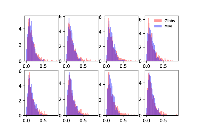
Figure 3: PG auxiliary variable $\omega_{i}$ by Gibbs sampling (red) and MIVI (blue) for eight randomly selected samples of the synthesized data in Section 4.2.

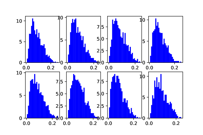
Figure 4: PG auxiliary variable $\omega_{i}$ by MIVI for eight randomly selected training images of the binary MNIST data in Section 4.2.

Appendix D Experiment settings

D.1 General settings

With the definitions of $J$ and $M$ in Algorithm 1, we run 1,000 epochs with $J=200$, $T=5$, and $M=100$ in the toy experiment of Section E.1 and 2,000 epochs with $J=1000$ and $M=0$ for the negative binomial model in Section 4.1. For the Bayesian logistic in Section 4.2 we run 1,000 epochs with $J=200$ and $M=0$. For the Bayesian bridge regression in Section 4.3 we run 1,000 epochs with $J=100$ and $M=0$. For the VAE by MIVI in Section 4.4 we run 2,500 epochs with $J=10$ and $M=200$.

For experiments of VAE on MNIST and FashionMNIST, we follow the original partition to split the data as 50,000/10,000/10,000 for training/validation/test. The MNIST data is dynamically binarized, and the FashionMNIST data is binarized with 0.5 as a threshold for each pixel. The dimension of the latent variable $\bm{z}$ is set as 40. To ensure the fairness of comparison, we use the same network architecture to build up the VAE on UIVI and VCD and use the same experiment configuration as in Titsias & Ruiz (2018) and Ruiz & Titsias (2019). We apply a 2-hidden-layer network with 200 hidden units for both encoder and decoder and choose ReLU as the activation function. Then we optimize the model using the initial learning rate as $0.001$ with a $10\%$ decay for every 15,000 iterations, and choose the best model with validation set for testing. Specifically for SIVI-VAE and DSIVI-VAE, the dimension of $\psi$ is set as 500. For MIVI we run $2,500$ epochs with the initial Adam learning rate as $0.001$ (with a $12\%$ decay for every 100 epochs) for MNIST and $0.0001$ (with a $10\%$ decay for every 200 epochs) for fMNIST.

D.2 Performance evaluation of MIVI on VAEs

In Section 4.4 we evaluate MIVI for VAEs by estimating the average marginal log-likelihood,

$$\log p(\tilde{\bm{x}})\approx\log\frac{1}{{\tilde{J}}}\sum_{j=1}^{\tilde{J}}\frac{p_{\theta}(\tilde{\bm{x}}\,|\,\bm{z}_{j})p(\bm{z}_{j})}{\tilde{q}_{\eta,\phi}(\bm{z}_{j})}=\log\frac{1}{{\tilde{J}}}\sum_{j=1}^{\tilde{J}}\frac{p_{\theta}(\tilde{\bm{x}}\,|\,\bm{z}_{j})p(\bm{z}_{j})}{q_{\phi}(\bm{z}_{j}\,|\,\tilde{\bm{x}})}e^{-D^{*}(\tilde{\bm{x}},\bm{z}_{j})}.$$

The correctness of right-hand side of this equation depends on an optimal discriminator $D^{*}$, which can be hard to verify. Therefore, we use the Gaussianity of SGLD and a Monte Carlo method to evaluate $\tilde{q}_{\eta,\phi}$. Specifically, the updating function of SGLD is $f_{\eta}(\bm{z},\epsilon)$ such that

$$\bm{z}^{(t)} =f_{\eta_{t}}(\bm{z}^{(t-1)},\epsilon_{t})$$

$$=\bm{z}^{(t-1)}+\frac{\eta_{t}}{2}\odot[\nabla_{\bm{z}}\log p(\bm{z}^{(t-1)})+\frac{N}{n}\nabla_{\bm{z}}\log p(\bm{x}\,|\,\bm{z}^{(t-1)})]+\epsilon_{t}$$

where $\epsilon_{t}\sim\mathcal{N}(\bm{0},\mbox{diag}(\eta_{t}))$ and $\odot$ stands for element-wise multiplication. So we have $\bm{z}^{(T)}\sim\mathcal{N}(\mu(\bm{z}^{(T-1)},\eta_{T}),\eta_{T})$ where $\mu(\bm{z},\eta)=\bm{z}+\frac{\eta}{2}\odot[\nabla_{\bm{z}}\log p(\bm{z})+\frac{N}{n}\nabla_{\bm{z}}\log p(\bm{x}\,|\,\bm{z})]$ and consequently,

$$\bm{z}^{(T)} \sim\mathcal{N}\left(\mu(\bm{z}^{(T-1)},\eta_{T}),\mbox{diag}(\eta_{T})\right)$$

$$=\mathcal{N}\left(\mu(f_{\eta_{T-1}}(\bm{z}^{(T-2)},\epsilon_{T-1}),\eta_{T-1}),\mbox{diag}(\eta_{T})\right)$$

$$=\mathcal{N}\left(\mu(f_{\eta_{T-1}}(f_{\eta_{T-2}}(\bm{z}^{(T-3)},\epsilon_{T-2}),\epsilon_{T-1}),\eta_{T-1}),\mbox{diag}(\eta_{T})\right)$$

$$=\mathcal{N}\left(\mu(f_{\eta_{T-1}}(f_{\eta_{T-2}}(\ldots(f_{\eta_{1}}(\bm{z}^{(0)},\epsilon_{1}),\epsilon_{2})\ldots),\epsilon_{T-1}),\mbox{diag}(\eta_{T})\right).$$

Therefore, the marginal distribution $\tilde{q}_{\eta,\phi}$ is equal to

$$\int\ldots\int\mathcal{N}\left(\mu(f_{\eta_{T-1}}(f_{\eta_{T-2}}(\ldots(f_{\eta_{1}}(\bm{z}^{(0)},\epsilon_{1}),\epsilon_{2})\ldots),\epsilon_{T-1})),\mbox{diag}(\eta_{T})\right)dP(\epsilon_{1})\ldots dP(\epsilon_{T-1})q_{\phi}(\bm{z}^{(0)})d\bm{z}^{(0)}$$

$$\approx \frac{1}{K}\sum_{k=1}^{K}\mathcal{N}\left(\mu(f_{\eta_{T-1}}(f_{\eta_{T-2}}(\ldots(f_{\eta_{1}}(\bm{z}^{(0)}_{k},\epsilon_{1,k}),\epsilon_{2,k})\ldots),\epsilon_{T-1,k})),\mbox{diag}(\eta_{T})\right)$$ (9)

where $\bm{z}_{k}^{(0)}\overset{iid}{\sim}q_{\phi}$, $\epsilon_{t,k}\overset{ind}{\sim}\mathcal{N}(0,\mbox{diag}(\eta_{t}))$ for $k=1,\ldots,K$ and $t=1,\ldots,T-1$. We evaluate the performance of MIVI for VAEs by

$$\log p(\tilde{\bm{x}}) \approx\log\frac{1}{{\tilde{J}}}\sum_{j=1}^{\tilde{J}}\frac{p_{\theta}(\tilde{\bm{x}}\,|\,\bm{z}_{j})p(\bm{z}_{j})}{\hat{q}_{\eta,\phi}(\bm{z}_{j})}$$ (10)

where $\bm{z}_{j}=f_{\eta_{T}}(f_{\eta_{T-1}}(\ldots(f_{\eta_{1}}(\bm{z}^{(0)}_{j},\epsilon_{1,j}),\epsilon_{2,j})\ldots),\epsilon_{T,j})$, $\bm{z}^{(0)}_{j}\overset{iid}{\sim}q_{\phi}$ and

$$\hat{q}_{\eta,\phi}(\bm{z}_{j})= \frac{1}{K+1}\mathcal{N}\left(\bm{z}_{j}\,|\,\mu(f_{\eta_{T-1}}(f_{\eta_{T-2}}(\ldots(f_{\eta_{1}}(\bm{z}^{(0)}_{j},\epsilon_{1,j}),\epsilon_{2,j})\ldots),\epsilon_{T-1,j})),\eta_{T}\right)+$$

$$\frac{1}{K+1}\sum_{k=1}^{K}\mathcal{N}\left(\bm{z}_{j}\,|\,\mu(f_{\eta_{T-1}}(f_{\eta_{T-2}}(\ldots(f_{\eta_{1}}(\bm{z}^{(0)}_{k},\epsilon_{1,k}),\epsilon_{2,k})\ldots),\epsilon_{T-1,k})),\eta_{T}\right)$$ (11)

analogous to Yin & Zhou (2018).

We set ${\tilde{J}}=1000$ and $K=50$ for the evaluation by the importance sampling. Note what we are estimating in (10) is in fact a lower bound of $\log p(\tilde{\bm{x}})$ (Burda et al., 2015). Its quality depends on both the decoder $p_{\theta}(\bm{x}\,|\,\bm{z})$ and the encoder which is used as the importance distribution; fixing $p_{\theta}(\bm{x}\,|\,\bm{z})$, a poor importance distribution may give rise to a loose bound. The estimation of MIVI-5-5 (using $\tilde{q}^{(T)}_{\eta,\phi}$ as the importance distribution) is better than that of MIVI-5-0 (using $q_{\phi}$ as the importance distribution) because $p_{\theta}(\bm{x}\,|\,\bm{z})$ is trained based on $\tilde{q}^{(T)}_{\eta,\phi}$. Moreover, in case of multimodality of $p(\bm{z}\,|\,\bm{x})$ which is very probable for VAE models, $q_{\phi}$ can be lighter-tailed than $\tilde{q}_{\eta,\phi}$ and may result in larger variance of the importance sampling estimation. In addition, we need be careful about extrapolation when conducting the importance sampling based estimation as in (10), which is only valid under the assumption that the importance distribution $q$ satisfies $q(\bm{z})>0$ when $p(\bm{x}\,|\,\bm{z})p(\bm{z})\neq 0$ (Owen, 2009). Concretely, though we have observed that the value obtained by (10) for MIVI-5-$t$ increases as $t$ grows, that value may no longer reflect the true performance of the model, since $\tilde{q}^{(t)}_{\eta,\phi}$ may no longer maintain non-negligible density on the regions where the joint likelihood has non-negligible values. So we only compare MIVI-5-5 so that the number of transitions are the same in training and testing.

Appendix E Supplimentary experimental results

E.1 Toy experiments

Table 2: Target bivariate distributions.

Correlated Gaussian Banana Gaussian mixture $\mathcal{N}\left(\begin{bmatrix}0\\ 0\end{bmatrix},\begin{bmatrix}1&0.8\\ 0.8&1\end{bmatrix}\right)$ $\mathcal{N}(z_{1};\frac{z_{2}^{2}}{4},1)\mathcal{N}(z_{2};0,4)$ $\frac{1}{2}\mathcal{N}\left(\begin{bmatrix}-1\\ -1\end{bmatrix},\begin{bmatrix}1&-0.5\\ -0.5&1\end{bmatrix}\right)+\frac{1}{2}\mathcal{N}\left(\begin{bmatrix}1.3\\ 1.3\end{bmatrix},\begin{bmatrix}1&0.3\\ 0.3&1\end{bmatrix}\right)$

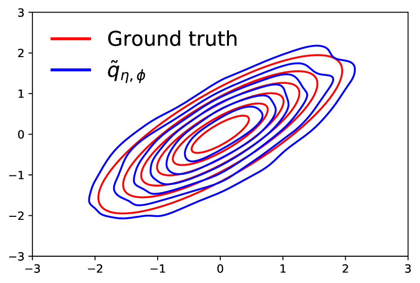
(a) Correlated Gaussian.

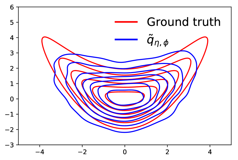
(b) Banana.

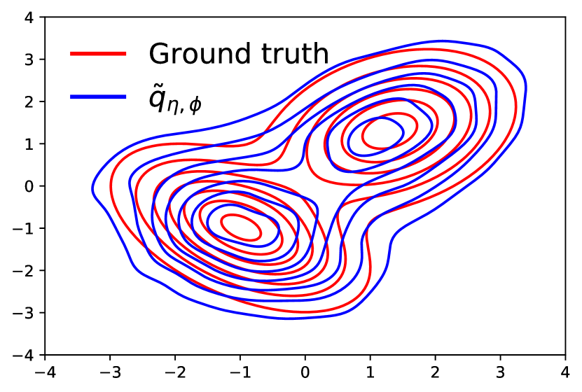
(c) Gaussian mixture.

Figure 5: Target distributions (red) and fitted $\tilde{q}_{\eta,\phi}$ (blue) of MIVI.

(a) Correlated Gaussian.

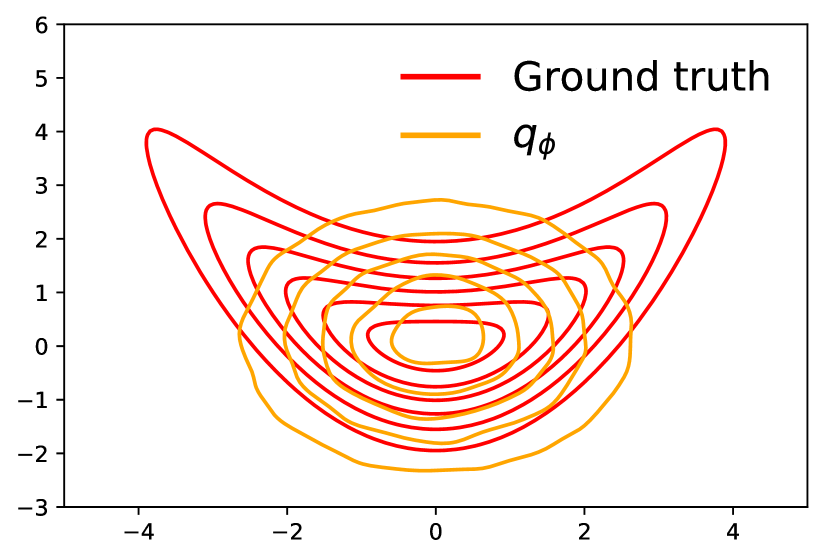
(b) Banana.

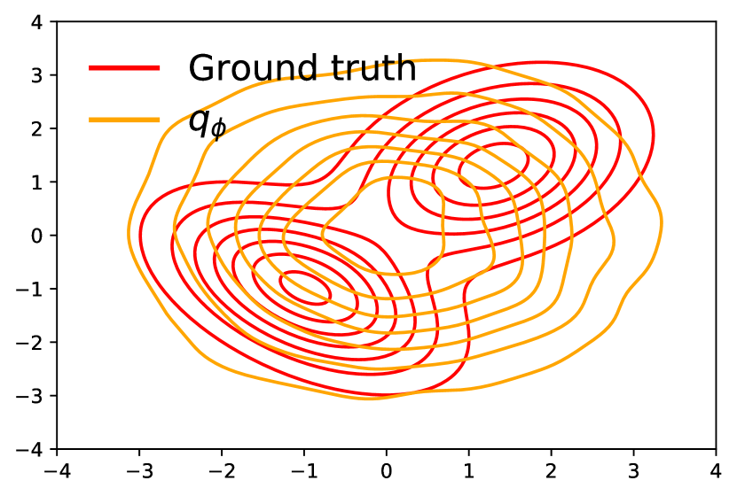
(c) Gaussian mixture.

Figure 6: Target distributions (red) and fitted $q_{\phi}$ (orange) of MIVI.

To show the validity and flexibility of $\tilde{q}_{\phi,\eta}$ of SGLD in MIVI, we fit synthetic bivariate distributions listed in Table 2. Figure 5 shows the contour plots of the synthetic bivariate distributions (red) along with the fitted $\tilde{q}_{\eta,\phi}(\bm{z})$ (blue). In all cases, $\tilde{q}_{\eta,\phi}(\bm{z})$ has well recovered the target distribution and captured the bivariate correlation, dependence, and multimodality, respectively, despite the small number of SGLD updates. In addition, Figure 6 shows that $q_{\phi}$ of MIVI has captured the large varianace of each dimension of $\bm{z}$.

E.2 Additional results of VAE

Table 3: Comparison of VAE algorithms on MNIST and fMNIST (${\textstyle\bm{z}\in\mathbb{R}^{10}}$).

Vanilla SIVI DSIVI UIVI VCD VIS-5-5 MIVI-5-0 MIVI-5-5 MNIST -97.82 -96.78 -89.96 -94.09 -95.86 -87.65 -92.04 -88.50 fMNIST -124.73 -121.42 -121.39 -110.72 -117.65 -116.27 -117.74 -113.17

We try a lower dimensional $\bm{z}$, set $\bm{z}\in\mathbb{R}^{10}$ in all models, keep other settings the same as in $\bm{z}\in\mathbb{R}^{40}$, and report the VAE model comparison in Table 3 where we cite the results of UIVI and VCD for $\bm{z}\in\mathbb{R}^{10}$ from Titsias & Ruiz (2018) and Ruiz & Titsias (2019), respectively. It is shown that MIVI-5-5 is as good as VIS-5-5 which also uses SGLD for a refined encoder, and outperforms implicit VI approaches (except UIVI on fMNIST) because MIVI’s encoder as in (11) is not only flexible but also less complex in parameterization and hence easy to optimize. We show reconstructions of randomly selected binarized MNIST testing images by MIVI in Figure 7 panel (a) and some of the most improved ones in panel (b). The first column is the testing image, the second column is the reconstruction using $\bm{z}\sim q_{\phi}$, and the third to the twelfth columns use $\bm{z}$ from $\tilde{q}_{\eta,\phi}^{(t)}$ for $t=1,\ldots,10$, respectively, with fine-tuned step sizes. Overall, the reconstructions are good enough by $\bm{z}\sim q_{\phi}$ and can be further improved by $\tilde{q}_{\eta,\phi}^{(t)}$ as $t$ increases.

(a) Randomly selected.

(b) Most improved.

Figure 7: VAE reconstructions of binarized MNIST testing images by MIVI ($\bm{z}\in\mathbb{R}^{10}$).

References

- Bierkens et al. (2019) Joris Bierkens, Paul Fearnhead, Gareth Roberts, et al. The Zig-Zag process and super-efficient sampling for Bayesian analysis of big data. The Annals of Statistics, 47(3):1288–1320, 2019.
- Blei et al. (2017) David M Blei, Alp Kucukelbir, and Jon D McAuliffe. Variational inference: A review for statisticians. Journal of the American Statistical Association, 112(518):859–877, 2017.
- Burda et al. (2015) Yuri Burda, Roger Grosse, and Ruslan Salakhutdinov. Importance weighted autoencoders. arXiv preprint arXiv:1509.00519, 2015.
- Chen et al. (2017) Changyou Chen, Chunyuan Li, Liqun Chen, Wenlin Wang, Yunchen Pu, and Lawrence Carin. Continuous-time flows for efficient inference and density estimation. arXiv preprint arXiv:1709.01179, 2017.
- Chen & Hwang (2013) Ting-Li Chen and Chii-Ruey Hwang. Accelerating reversible Markov chains. Statistics & Probability Letters, 83(9):1956–1962, 2013.
- Cover & Thomas (2006) Thomas M Cover and Joy A Thomas. Elements of information theory 2nd edition (Wiley series in Telecommunications and Signal Processing), 2006.
- de Freitas et al. (2001) Nando de Freitas, Pedro Højen-Sørensen, Michael I Jordan, and Stuart Russell. Variational MCMC. In Proceedings of the Seventeenth Conference on Uncertainty in Artificial Intelligence, UAI’01, pp. 120–127, San Francisco, CA, USA, 2001. Morgan Kaufmann Publishers Inc. ISBN 1558608001.
- Ding et al. (2014) Nan Ding, Youhan Fang, Ryan Babbush, Changyou Chen, Robert D Skeel, and Hartmut Neven. Bayesian sampling using stochastic gradient thermostats. In Advances in Neural Information Processing Systems, pp. 3203–3211, 2014.
- Efron et al. (2004) Bradley Efron, Trevor Hastie, Iain Johnstone, Robert Tibshirani, et al. Least angle regression. The Annals of Statistics, 32(2):407–499, 2004.
- Gallego & Insua (2019) Victor Gallego and David Ríos Insua. Variationally inferred sampling through a refined bound for probabilistic programs. arXiv preprint arXiv:1908.09744, 2019.
- Geman & Geman (1984) Stuart Geman and Donald Geman. Stochastic relaxation, Gibbs distributions, and the Bayesian restoration of images. IEEE Transactions on Pattern Analysis and Machine Intelligence, 6:721–741, 1984.
- Habib & Barber (2019) Raza Habib and David Barber. Auxiliary variational MCMC. the International Conference on Learning Representations (ICLR), 2019.
- Hastings (1970) WK Hastings. Monte Carlo sampling methods using markov chains and their applications. Biometrika, 57(1):97–109, 1970.
- Hoffman (2017) Matthew D Hoffman. Learning deep latent gaussian models with markov chain monte carlo. In International Conference on Machine Learning, pp. 1510–1519, 2017.
- Jordan et al. (1999) Michael I Jordan, Zoubin Ghahramani, Tommi S Jaakkola, and Lawrence K Saul. An introduction to variational methods for graphical models. Machine Learning, 37(2):183–233, 1999.
- Khasminskii (2011) Rafail Khasminskii. Stochastic stability of differential equations, volume 66. Springer Science & Business Media, 2011.
- Kingma & Ba (2014) Diederik P Kingma and Jimmy Ba. Adam: A method for stochastic optimization. arXiv preprint arXiv:1412.6980, 2014.
- Kingma & Welling (2014) Diederik P Kingma and Max Welling. Auto-encoding variational Bayes. In the International Conference on Learning Representations (ICLR), 2014.
- Le et al. (2018) Tuan Anh Le, Maximilian Igl, Tom Rainforth, Tom Jin, and Frank Wood. Auto-encoding sequential Monte Carlo. In International Conference on Learning Representations (ICLR), 2018.
- Li et al. (2016) Chunyuan Li, Changyou Chen, David Carlson, and Lawrence Carin. Preconditioned stochastic gradient Langevin dynamics for deep neural networks. In 30th AAAI Conference on Artificial Intelligence, 2016.
- Li et al. (2017) Yingzhen Li, Richard E Turner, and Qiang Liu. Approximate inference with amortised MCMC. arXiv preprint arXiv:1702.08343, 2017.
- Ma et al. (2015) Yi-An Ma, Tianqi Chen, and Emily Fox. A complete recipe for stochastic gradient MCMC. In Advances in Neural Information Processing Systems, pp. 2917–2925, 2015.
- Maddison et al. (2017) Chris J Maddison, John Lawson, George Tucker, Nicolas Heess, Mohammad Norouzi, Andriy Mnih, Arnaud Doucet, and Yee Teh. Filtering variational objectives. In Advances in Neural Information Processing Systems, pp. 6573–6583, 2017.
- Mescheder et al. (2017) Lars Mescheder, Sebastian Nowozin, and Andreas Geiger. Adversarial variational Bayes: Unifying variational autoencoders and generative adversarial networks. In Proceedings of the 34th International Conference on Machine Learning, pp. 2391–2400, 2017.
- Metropolis et al. (1953) Nicholas Metropolis, Arianna W Rosenbluth, Marshall N Rosenbluth, Augusta H Teller, and Edward Teller. Equation of state calculations by fast computing machines. The Journal of Chemical Physics, 21(6):1087–1092, 1953.
- Molchanov et al. (2019) Dmitry Molchanov, Valery Kharitonov, Artem Sobolev, and Dmitry Vetrov. Doubly semi-implicit variational inference. International Conference on Artificial Intelligence and Statistics, 2019.
- Naesseth et al. (2018) Christian Naesseth, Scott Linderman, Rajesh Ranganath, and David Blei. Variational sequential Monte Carlo. In International Conference on Artificial Intelligence and Statistics, pp. 968–977, 2018.
- Neal (1998) Radford M Neal. Suppressing random walks in Markov Chain Monte Carlo using ordered overrelaxation. In Learning in Graphical Models, pp. 205–228. Springer, 1998.
- Nijkamp et al. (2020) Erik Nijkamp, Bo Pang, Tian Han, Linqi Zhou, Song-Chun Zhu, and Ying Nian Wu. Learning multi-layer latent variable model via variational optimization of short run MCMC for approximate inference. arXiv:1912.01909, 2020.
- Owen (2009) Art B Owen. Importance sampling. Monte Carlo Theory, methods and examples.: http://statweb. stanford. edu/~ owen/mc/Ch-var-is. pdf, 2009.
- Park & Casella (2008) Trevor Park and George Casella. The Bayesian lasso. Journal of the American Statistical Association, 103(482):681–686, 2008.
- Polson et al. (2013) Nicholas G Polson, James G Scott, and Jesse Windle. Bayesian inference for logistic models using Pólya–gamma latent variables. Journal of the American statistical Association, 108(504):1339–1349, 2013.
- Polson et al. (2014) Nicholas G Polson, James G Scott, and Jesse Windle. The Bayesian bridge. Journal of the Royal Statistical Society: Series B (Statistical Methodology), 76(4):713–733, 2014.
- Ranganath et al. (2016) Rajesh Ranganath, Dustin Tran, and David Blei. Hierarchical variational models. In International Conference on Machine Learning, pp. 324–333, 2016.
- Rezende & Mohamed (2015) Danilo Rezende and Shakir Mohamed. Variational inference with normalizing flows. volume 37 of Proceedings of Machine Learning Research, pp. 1530–1538, 2015.
- Robert et al. (2018) Christian P Robert, Víctor Elvira, Nick Tawn, and Changye Wu. Accelerating MCMC algorithms. Wiley Interdisciplinary Reviews: Computational Statistics, 10(5):e1435, 2018.
- Ruiz & Titsias (2019) Francisco JR Ruiz and Michalis K Titsias. A contrastive divergence for combining variational inference and MCMC. In Proceedings of the 28th International Conference on Machine Learning (ICML-19), 2019.
- Salakhutdinov & Murray (2008) Ruslan Salakhutdinov and Iain Murray. On the quantitative analysis of deep belief networks. In Proceedings of the 25th International Conference on Machine Learning, pp. 872–879, 2008.
- Salimans et al. (2015) Tim Salimans, Diederik Kingma, and Max Welling. Markov Chain Monte Carlo and variational inference: Bridging the gap. In International Conference on Machine Learning, pp. 1218–1226, 2015.
- Teh et al. (2016) Yee Whye Teh, Alexandre H Thiery, and Sebastian J Vollmer. Consistency and fluctuations for stochastic gradient langevin dynamics. The Journal of Machine Learning Research, 17(1):193–225, 2016.
- Titsias (2017) Michalis K Titsias. Learning model reparametrizations: Implicit variational inference by fitting MCMC distributions. arXiv preprint arXiv:1708.01529, 2017.
- Titsias & Ruiz (2018) Michalis K Titsias and Francisco JR Ruiz. Unbiased implicit variational inference. arXiv preprint arXiv:1808.02078, 2018.
- Tran et al. (2017) Dustin Tran, Rajesh Ranganath, and David Blei. Hierarchical implicit models and likelihood-free variational inference. In Advances in Neural Information Processing Systems, pp. 5523–5533, 2017.
- Vollmer et al. (2016) Sebastian J Vollmer, Konstantinos C Zygalakis, and Yee Whye Teh. Exploration of the (non-) asymptotic bias and variance of stochastic gradient langevin dynamics. The Journal of Machine Learning Research, 17(1):5504–5548, 2016.
- Welling & Teh (2011) Max Welling and Yee W Teh. Bayesian learning via stochastic gradient Langevin dynamics. In Proceedings of the 28th International Conference on Machine Learning (ICML-11), pp. 681–688, 2011.
- West (1987) Mike West. On scale mixtures of normal distributions. Biometrika, 74(3):646–648, 1987.
- Xiao et al. (2017) Han Xiao, Kashif Rasul, and Roland Vollgraf. Fashion-MNIST: A novel image dataset for benchmarking machine learning algorithms. arXiv preprint arXiv:1708.07747, 2017.
- Yin & Zhou (2018) Mingzhang Yin and Mingyuan Zhou. Semi-implicit variational inference. In Proceedings of the 28th International Conference on Machine Learning (ICML-18), 2018.
- Zhang et al. (2020) Yichuan Zhang, José Miguel Hernández-Lobato, and Zoubin Ghahramani. Ergodic measure preserving flows. the International Conference on Learning Representations (ICLR), 2020.
- Zhou et al. (2012) Mingyuan Zhou, Lingbo Li, David Dunson, and Lawrence Carin. Lognormal and gamma mixed negative binomial regression. In Proceedings of the International Conference on Machine Learning, volume 2012, pp. 1343, 2012.