Locally refined spline surfaces for terrain and sea bed data: tailored approximation, export and analysis tools

Abstract

The novel Locally Refined B-spline (LR B-spline) surface format is suited for representing terrain and seabed data in a compact way. It provides an alternative to the well know raster and triangulated surface representations. An LR B-spline surface has an overall smooth behaviour and allows the modelling of local details with only a limited growth in data volume. In regions where many data points belong to the same smooth area LR B-splines allow a very lean representation of the shape by locally adapting the resolution of the spline space to the size and local shape variations of the region. The surfaces generated approximate the smooth component of a cloud of data points within user specified tolerances. The method can be modified to improve the accuracy in particular domains and selected data points. The resulting surfaces are well suited for analysis and computing secondary information such as contour curves and minimum and maximum points. The surfaces can be translated into a raster or a tessellated surface of desired quality or exported as collections of tensor product spline surfaces. Data transfer can also be performed using Part 42 of ISO 10303 (the STEP standard) where LR B-splines were published in 2018.

Funding This work has been supported by the Norwegian research counsil under grant number 270922.

Acknowledgements The Norwegian map authorities, division Sjøkartverket has provided the measurement data.

1 Introduction

Geospatial data acquisition of terrains and sea beds produces huge point clouds. The structure, or lack of structure, in the point cloud depends on the actual data acquisition technology used. Efficient downstream uses of the acquired data require in general structured and compact data representations. Working directly in the point cloud is not attractive.

The approach we follow in this paper is to use the novel Locally Refined B-spline surfaces (LR B-splines) for representation of geospatial data. To relate LR B-splines to surface representations already in use in Geographic Information Systems (GIS), we provide in Section 2 an overview of other relevant representations.

The starting point for an LR B-spline surface is a tensor product B-spline surface. In the LR B-spline surface extra degrees of freedom are inserted locally when needed. The desired smoothness is maintained, and the growth in data volume is kept under control. The extension of tensor product B-spline surfaces to LR B-splines is presented in detail in Section 3. A summary and comparison of the presented surface representation formats is given in Section 4. Section 5 presents the procedure for creating LR B-spline surfaces from geographical point clouds. Section 5 also include an example where we compare approximation with LR B-spline surfaces and raster representations of the same point cloud.

Interoperability with existing GIS-technology is essential for the deployment of LR B-splines within GIS. Section 6 addresses how LR B-spline surfaces can be converted to standard formats used in GIS-systems.

Once an LR B-spline surface representation of some GIS data is obtained, this surface can be interrogated and analyzed to compute and derive terrain information, e.g., contour curves, slope and aspect ratio. In Section 7 we focus on contour curves and extremal points.

The format of locally refined splines is flexible. The property of local refinement is used to expand the modelling freedom in areas with high degree of local variation in the data set. This flexibility can be exploited further by requiring higher accuracy in specified areas or in selected points. In the subsea context it is most often important to have high accuracy in areas with shallow water rather than where the water is deep. Section 8 looks into three different methods to emphasize particular domains in the data set.

Finally, we will provide some conclusions and set directions for further work in Section 9.

2 GIS surface representations

Representation of terrain phenomena has been a topic for a long time and not less so in the digital era. Different aspects with digital terrain modelling is discussed in terrain . Among the topics are representation of digital terrain model surfaces and quality assessment.

Spatial interpolation is the process of using points with known values to estimate values at unknown sample points. The corresponding interpolator can be exact or approximative depending on whether or not the initial data points are fitted exactly. In the context of large geospatial data sets only approximative interpolators are feasible. Methods using all data points to estimate a sample point are global, while methods using a subset of points are local. A survey on interpolation methods can be found in GISinterpolation .

Most GIS systems offer the possibility of the Inverse distance weighting interpolation (IDW) method originally proposed by Shepard, see IDW . The method is simple, but tends to create flat spots around sparse data points. Initially IDW was a global method, but modifications have been proposed to define sample points from subsets of data and to avoid flat spots AltShepard ; ShepardLim .

Natural neighbour interpolation NNneighbour is originally based on Voronoi tessellation and tends to give a more smooth result than the Inverse distance weighting. Kriging Kriging is an advanced technique using a Geo-statistical approach where the estimation errors are directly available. Kriging is a weighted average technique where all data points are analyzed to find the auto-correlation of the particular data set being interpolated. Radial basis functions (RBF) provide another set of methods for scattered data interpolation. Originally a global method resulting in equation systems of the same size as the number of data points but local methods have also been developed LocalRBF . Several types of basis functions are used in the context of RBF, and Franke evaluated of some functions in RBFTest . Buhmann discusses radial basis functions and properties thereof in radial .

In contrast to the previously presented methods the use of splines in GIS interpolation can result in sample values outside the convex hull of the data points. This restrains the smoothing effect inherent in those methods and enables the estimation of lows and highs not present in the input data, but may result in exaggerated behaviour, in particular if the data points are close and have extreme differences in value. Splines in GIS most often mean splines in tension or regularized splines, see GISinterpolation , which differ from the tensor product splines presented in Section 3.2.

The raster representation is the most frequently used data format in GIS. To make a raster representation of a point cloud, spatial interpolation is used to define values, for instance elevation or precipitation, in a regular grid. The digital elevation model (DEM), which is a raster representation, is the most commonly used format for processed terrain and sea bed data. The raster is a compact, highly structured and efficient representation. It is also an approximate representation as the input data are not exactly fitted. The accuracy depends on the resolution of the raster and the selected interpolation method. If the resolution is low compared to the variation of the data then the result will be inaccurate, if it is high then the data volume grows more than necessary. If there are large differences in the local variation of the data in different areas, then a trade-off between accuracy and data volume must be made.

A raster represented surface is not completely defined by the sample points. Given a raster the interpolation method is often unknown, and values between the sample values have to be estimated. Several approaches are available. The value in the cell center may be selected. Another simple method is bivariate evaluation where the estimated value is computed from a bivariate surface interpolating the four surrounding sample values. Inverse distance weighting and other interpolation methods can be used also in this context.

Root mean square error (RMSE) is the standard way of measuring the error of a model. $RMSE=\sqrt{\frac{\sum_{i=1}^{n}(\hat{z}_{i}-z_{i})^{2}}{n}}$, where $n$ is the number of data values, $z_{i}$ are the given values and $\hat{z}_{i}$ are the corresponding estimated values. RMSE is a good measure if we want to estimate the standard deviation $\sigma$ of a typical observed value from our model’s prediction, assuming that our observed data can be decomposed into the predicted value and random noise with mean zero. It does not, however, take the spatial pattern of the error into account. Fisher and Tate discuss errors in digital elevation models in ErrDEM1 . Different interpolation methods are considered without giving one clear recommendation. The accuracy of which a given terrain is approximated with a DEM depends on the match between the DEM resolution and the terrain features. Wise investigates the relation between terrain types and DEM error in ErrDEM2 and evaluates five interpolation methods (bilinear, IDW, RBF, spline and local polynomial) in the context of re-sampling in ErrDEM3 . The effect on derivative information such as slope is also studied. Splines and RBF is found to give the best results. He also finds a link between the characteristics of the terrain and the pattern of errors in elevation.

A triangulated irregular network (TIN) is a continuous surface representation frequently used in GIS. This is a flexible format for geospatial data that allows adaptation to local variations. It is thus capable of very high accuracy. In TINbasin a triangulated surface is used to represent a drainage-basins while hydrological similarity is used in the TIN creation in TINhydro . To restrict the data size, approximation is required also here. However, the nodes of a TIN are distributed variably to create an accurate representation of the terrain. TINs can, thus, have a higher resolution in areas where a surface is highly variable or where more detail is desired and a lower resolution in areas that are less variable.

TIN models have a more complex data structure than raster surface models and tend to be more expensive to build and process. Therefore TINs are typically used for high-precision modelling of smaller areas. The triangulated surface consists of flat triangles. Points in-between the corner points in a triangle are found by linear interpolation, which can give a jagged appearance of the surface. The problem is especially visible at sharp or nearly sharp edges, but can be remedied by methods like constrained Delaunay triangulation. However, conforming Delaunay triangulation is often recommended over constrained triangulation due to less propensity to create long, skinny triangles, which are undesirable for surface analysis. In terrain a comprehensive discussion on various aspects with triangulation in terrain modelling is presented.

3 B-splines and locally refined splines

Within Computer-Aided Design (CAD) the univariate minimal support B-splines basis is used for the representation of B-spline spline curves. For the representation of tensor product B-spline surfaces in CAD a basis generated by the tensor product of two univariate minimal support B-splines bases is used. In the context of CAD the term ”B-spline basis function” is often used, this is valid for the minimal support bases described above. However, when building locally refined spline spaces for T-splines and Locally refined B-splines we risk, if care is not taken, to end up with a collection of tensor product B-splines spanning the spline space, that is not linearly independent. Consequently the collection of tensor product B-splines that span the spline space will not always constitute a basis for the B-spline space spanned. To explain Locally Refined B-splines we need to recap a number of B-spline basics. In Section 3.1 we address a single B-spline, the tensor product of two B-splines, the univariate minimal support B-spline bases and the bivariate minimal support tensor product B-spline basis. Then we address B-spline curves and tensor product B-splines surfaces in Section 3.2, and locally refined B-spline surfaces in 3.3.

3.1 B-splines, tensor product B-splines and minimal support B-spline bases

Given a non-decreasing sequence $\mathbf{u}=(u_{0},u_{1},\ldots,u_{p+1})$ we define a B-spline $B[\mathbf{u}]:{\mathbb{R}}\to{\mathbb{R}}$ of degree $p\geq 0$ recursively as follows

$$B[\mathbf{u}](u):=\frac{u-u_{0}}{u_{p}-u_{0}}B[u_{0},\ldots,u_{p}](u)+\frac{u_{p+1}-u}{u_{p+1}-u_{1}}B[u_{1},\ldots,u_{p+1}](u),$$ (1)

starting with

$$B[u_{i},u_{i+1}](u):=\begin{cases}1;&\text{if $u_{i}\leq u<u_{i+1}$};\\ 0;&\text{otherwise},\end{cases}\quad i=0,\ldots,p.$$

We define $B[\mathbf{u}]\equiv 0$ if $u_{p+1}=u_{0}$ and terms with zero denominator are defined to be zero.

A univariate spline space can be defined by a polynomial degree $p$ and a knot vector $\mathbf{u}=\{u_{0},u_{2},\ldots,u_{N+p}\}$, where the knots satisfy: $u_{i+1}\geq u_{i}$, $i=0,\ldots,N+p-1$, and $u_{i+p+1}>u_{i}$, $i=0,\ldots,N-1$. I.e, a knot value can be repeated $p+1$ times. The number of times a knot value is repeated is called the multiplicity $m$ of the knot value. The continuity across a knot value of multiplicity $m$ is $C^{p-m}$.

A basis for the univariate spline space above can be defined in many ways. However, the approach most often used is the univariate minimal support B-spline basis. In this the B-splines are defined by selecting $p+2$ consecutive knots from $\mathbf{u}$, starting from the first knot. So $B_{i,p}(u):=B[u_{i},\ldots,u_{i+p+1}](u)$ is defined by the knots $u_{i},\ldots,u_{i+p+1}$, $i=0,\ldots,N-1$ . The minimal support B-spline basis has useful properties such as local support, non-negativity and partition of unity (the basis functions sum up to one in all parameter values in the interval $[u_{p},u_{N}]$).

Given two non-decreasing knot sequences $\mathbf{u}=\{u_{0},u_{1},\ldots,u_{N_{1}+p_{1}}\}$ and $\mathbf{v}=\{v_{0},v_{1},\ldots,v_{N_{2}+p_{2}}\}$ where $p_{1}\geq 0$ and $p_{2}\geq 0$. We define a bivariate tensor product B-spline $B_{i,j,p_{1},p_{2}}:{\mathbb{R}^{2}}\to{\mathbb{R}}$ from the two univariate B-splines $B_{i,p_{1}}(u)$ and $B_{j,p_{2}}(v)$ by

$$B_{i,j,p_{1},p_{2}}(u,v):=B_{i,p_{1}}(u)B_{j,p_{2}}(v).$$

The support of $B$ is given by the cartesian product

$$\text{\em supp}(B_{i,j,p_{1},p_{2}}):=[u_{i},u_{i+p_{1}+1}]\times[v_{j},v_{j+p_{2}+1}].$$

A bivariate tensor product spline space is made by the tensor product of two univariate spline spaces. Assuming that both univariate spline spaces have a minimal support B-spline basis, the minimal support basis for the tensor product B-spline space is constructed by making all tensor product combinations of the B-splines of the two bases. The minimal support basis for this spline space contains the tensor product B-splines $B_{i,j,p_{1},p_{2}}(u,v)$, $i=0,\ldots,N_{1}-1$, $j=0,\ldots,N_{2}-1$. As in the univariate case the basis has useful properties such as non-negativity and partition of unity.

3.2 B-spline curves and tensor product B-spline surfaces

Spline curves are frequently represented using a univariate minimal support B-spline basis.

$$f(u)=\sum_{i=0}^{N-1}c_{i}B_{i,p}(u),u\in[u_{p},u_{N}].$$ (2)

Here $c_{i}\in R^{d}$, $i=0,\ldots,N-1$ are the curve coefficients and $d$ is the dimension of the geometry space. The curve lies in the convex hull of its coefficients.

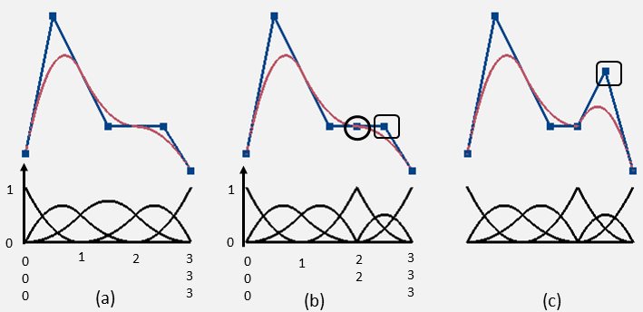
Figure 1: Knot insertion into a quadratic B-spline curve. (a) Initial curve with basis functions, (b) curve and basis functions after knot insertion, (c) curve and basis functions after re-positioning of one coefficient

A B-spline curve can be locally refined. Fig. 1 (a) shows a quadratic curve with knot vector ${\{0,0,0,1,2,3,3,3\}}$. The curve coefficients and the control polygon corresponding to the curve are included in the figure, and the associated B-splines are shown below. In (b) a new knot with value $2$ is added, thus increasing the knot multiplicity in an already existing knot. The curve is not altered, but the control polygon is enhanced with a new coefficient interpolating the curve. The coefficient is marked with a circle in Fig. 1 (b). The double knot at $2$ allows creating a curve with $C^{0}$ continuity. When moving the coefficient marked with a square, we obtain a sharp corner (c). Note that only the last part of the curve is modified.

Spline surfaces are frequently represented using a bivariate minimal support tensor product B-spline basis.

$$F(u,v)=\sum_{i=0}^{N_{1}-1}\sum_{j=0}^{N_{2}-1}c_{i,j}B_{i,j,p_{1},p_{2}}(u,v)\in[u_{p_{1}},u_{N_{1}}]\times[v_{p_{2}},v_{N_{2}}].$$ (3)

Here $c_{i,j}\in R^{d}$, $i=0,\ldots,N_{1}-1$, $j=0,\ldots,N_{2}-1$ are the surface coefficients and $d$ is the dimension of the geometry space.

The construction of the basis functions implies that the properties of the univariate B-spline basis functions carry over to the tensor product case, implying that the tensor product spline surface is a stable construction. Fig. 2 shows an example of a tensor product B-spline with the knot vector ${\{0,1,2,3\}}$ in both parameter directions.

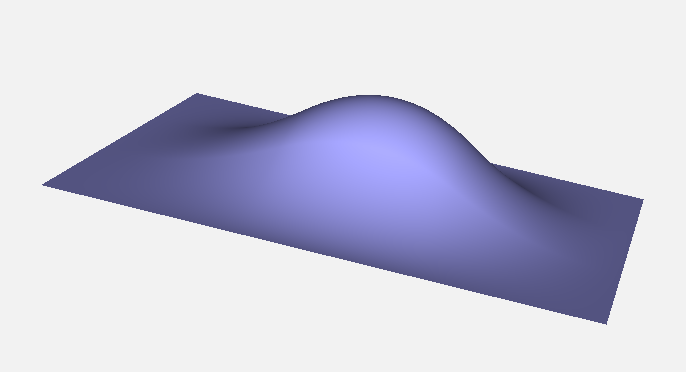
Figure 2: Example of a bi-quadratic tensor product B-spline basis functions.

Tensor product B-spline surfaces lack the property of local refinement. The distance between consecutive knots may differ so the size of the polynomial pieces may vary and increased knot multiplicity decreases the continuity between adjacent polynomial segments. However, a knotline cannot be restricted to only a part of the surface. If one new knot is inserted in the first parameter direction of the surface (3) the number of coefficients will increase with $N_{2}$.

3.3 Locally refined B-spline surfaces

In some applications such as representation of terrain and sea bed, the lack of local refinement is a severe restriction. A tensor product surface covers a rectangular domain and the need for approximation power will not be uniformly distributed throughout this domain. There are three main approaches for extending spline surfaces to support local refinement compared in trivariate .

• Hierarchical B-splines hierarchical are based on a dyadic sequence of grids determined by scaled lattices. On each level of the dynastic grids a spline space spanned by uniform tensor product B-spines is defined. The refinement is performed one level at the time. Tensor product B-splines on the coarser level are removed and B-splines at the finer level added in such a way that linear independence is guaranteed. The sequence of spline space for Hierarchical B-splines will be nested.

• T-splines tsplines denote a class of locally refined splines, most often presented using bi-degree $(3,3)$. The starting point for T-spline refinement is a tensor product B-spline surface with control points and meshlines (initial T-mesh) with assigned knot values. For a bi-degree (3,3) T-splines the knot vectors of the tensor product B-spline corresponding to a control point is determined by moving in the T-mesh outwards from the control point in all four axis parallel parameter directions and picking in each direction knot values from the two first T-mesh lines intersected. The mid knot value in each knot vector is copied from the control point. The refinement is performed by successively adding new control points in-between two adjacent control points in the T-mesh. The control point inherits one parameter value from the T-mesh line. The other parameter is chosen so that sequence of control point parameter values have a monotone evolution along the T-mesh line. Control points on adjacent parallel T-mesh lines that have one shared parameter value are connected with a new T-mesh line. The general formulation of T-splines does not guarantee a sequence of nested spline spaces and that the polynomial space is spanned over each element. However, T-spline subtypes such as semi-standard T-splines and Analysis Suitable T-splines AST do.

• Locally Refined B-splines lrsplines , the refinement approach of this paper, starts (as T-splines) from a tensor product B-spline surface. The refinement is performed successively by inserting axis parallel meshlines in the mesh of knotlines. Each meshline inserted has to split the support of at at least one tensor product B-spline. The constant knot value of a meshline inserted is used for performing univariate knot insertion. The refinement is performed in the parameter direction orthogonal to the meshline in all tensor product B-splines that have a support split by the meshline. This approach ensures that the spline spaces produced are nested and that the polynomial space is spanned over all polynomial elements. In Section 3.3.2 we provide further details on additional refinements triggered and how the resulting tensor product B-splines can be scaled to achieve partition of unity.

3.3.1 Preparing the tensor product B-spline surface for local refinement

After the first local refinement is performed on the initial tensor product B-splines surface the regular mesh structure is lost. The representation in Equation 3, where the local knot vectors are described by an index pointing into a global knot array and the polynomial degree, is no longer applicable. We now organize the tensor product B-splines, each now knowing its local knot vectors, as a collection of B-splines $\mathcal{B}_{0}$. Doing this we can represent the tensor product surface in Equation 3 by setting $\mathcal{B}_{j}=\mathcal{B}_{0}$.

$$F(u,v)=\sum_{B\in\mathcal{B}_{j}}c_{B}s_{B}B(u,v).$$ (4)

Here $c_{B}$ is the coefficient corresponding to the B-spline $B$. We have added a scaling factor $s_{B}$ to each tensor product B-spline. This is used for recording how the collection of tensor product B-splines generated during the refinement have to be scaled to form a positive partition of unity. For a tensor product B-spline surface all $s_{B}\equiv 1$. Using the representation we can remove B-splines to be refined by knot insertion from the collection and replace them with the refined B-splines and a scaling factor that provides a scaled partition of unity. Note that the same tensor product B-spline can result from the refinement of different B-splines. Consequently duplicates have to be identified and their scaling factors accumulated.

3.3.2 LR B-spline refinement

The process of Locally Refine B-splines (LR B-splines) is described in detail in lrsplines . Please consult the paper for formal proofs. Below a summary of the most important steps is presented. The refinement always starts from a tensor product B-spline space represented as in Equation 4. The refinement proceeds with a sequence of meshline insertions producing a series of collections of tensor product B-splines $\mathcal{B}_{0},\mathcal{B}_{1},\ldots,\mathcal{B}_{j},\mathcal{B}_{j+1}$ spanning nested spline spaces. Note that we require that all tensor product B-splines in these collection have minimal support. By this we mean that all meshlines that cross the support of a tensor product B-spline also have to be a knotline of the tensor product B-splines counting multiplicity. Thus, to ensure that all tensor product B-splines have this property the process of going from $\mathcal{B}_{j}$ to $\mathcal{B}_{j+1}$ frequently includes a number of steps and a sequence of LR B-spline collections $\mathcal{B}_{j,1},\mathcal{B}_{j,2},\ldots,\mathcal{B}_{j,r_{j}}$, where $\mathcal{B}_{j,1}=\mathcal{B}_{j}$ and $\mathcal{B}_{j,r_{j}}=\mathcal{B}_{j+1}$.

Assume that Equation 4 represents $F(u,v)$ using the collection $\mathcal{B}_{j}$ and we now want to represent $F(u,v)$ after refining with a given meshline to produce a refined representation of $F(u,v)$. The refinement process goes as follows:

• As long as there is a $B\in\mathcal{B}_{j}$ that does not have minimal support on the refined mesh we proceed as follows. Let $\gamma$ be a meshline that splits the support of $B$. This means that either $\gamma$ is not a knotline of $B$, or $\gamma$ is a knotline of $B$ but has higher multiplicity than the knotline of $B$. Decompose $B$ into its univariate component B-splines $B(u,v)=B(u)B(v)$. We now have two cases:

  • If $\gamma$ is parallel to second parameter direction then it has a constant parameter value $a$ in the first parameter direction. We insert $a$ in the univariate B-spline $B(u)$ using Equation 6 below and express $B(u)$ as $B(u)=\alpha_{1}B_{1}(u)+\alpha_{2}B_{2}(u)$. Then we make two new tensor product B-splines $B_{1}(u,v)=B_{1}(u)B(v)$ and $B_{2}(u,v)=B_{2}(u)B(v)$.

  • If $\gamma$ is parallel to first parameter direction then it has a constant parameter value $a$ in the second parameter direction. We insert $a$ in the univariate B-spline $B(v)$ using Equation 6 below and express $B(v)$ as $B(v)=\alpha_{1}B_{1}(v)+\alpha_{2}B_{2}(v)$. Then we make the two new tensor product B-splines $B_{1}(u,v)=B(u)B_{1}(v)$ and $B_{2}(u,v)=B(u)B_{2}(v)$.

  $B$ can now be decomposed as follows, $B(u,v)=\alpha_{1}B_{1}(u,v)+\alpha_{2}B_{2}(u,v)$. We can now express $F(u,v)$ by replacing $B(u,v)$ with the two new tensor product B-splines. $F(u,v)=F(u,v)-c_{B}s_{B}B(u,v)+c_{B}s_{B}(\alpha_{1}B_{1}(x,y)+\alpha_{2}B_{2}(x,y))$. We update $\mathcal{B}_{j}$ by removing $B$ and adding the tensor product B-splines $B_{1}(u,v)$ and $B_{2}(u,v)$. In addition we have to create/update both coefficients and scaling factors belonging to these two tensor product B-splines. We must have in mind that $B_{1}(x,y)$ and $B_{2}(x,y)$ often will be duplicates of B-splines already in $\mathcal{B}_{j}$. Now let $B_{r},r=1,2$

  • In the case $B_{r}$ has no duplicate set $s_{B_{r}}=s_{B}\alpha_{r}$ and $c_{B_{r}}=c_{B}$.

  • In the case $B_{r}$ has a duplicate $B_{d}$ set $s_{B_{r}}=s_{B_{d}}+s_{B}\alpha_{r}$ and $c_{B_{r}}=({s_{B_{d}}c_{B_{d}}+s_{B}\alpha_{r}c_{B}})/({s_{B_{r}}})$, and remove the duplicate.

  Note that $s_{B}$, $\alpha_{r}$ and $s_{B_{d}}$ are all positive numbers, thus $s_{B_{r}}$ will be positive.

  When all $B\in\mathcal{B}_{j}$ have minimal support we set $\mathcal{B}_{j+1}=\mathcal{B}_{j}$.

We now define the scaled tensor product B-splines $N_{B}(u,v)=s_{B}B(u,v)$ to provide a basis that is partition of unity for the spline space spanned by $\mathcal{B}_{j}$. If $F(x,y)\equiv 1$ then all coefficients of the tensor product B-spline surface we start from are $1$. In this case the coefficients $c_{B_{r}}$ calculated above all remain $1$, duplicates or not. Consequently,

$$\sum_{B\in\mathcal{B}_{j}}N_{B}(u,v)=\sum_{B\in\mathcal{B}_{j}}s_{B}B(u,v)=\sum_{B\in\mathcal{B}_{0}}B(u,v)=1.$$ (5)

.

The process of inserting a knot $a\in(u_{0},u_{p+1})$ into the local knot vector $[{\mathbf{u}}]=\{u_{0},\ldots,u_{p+1}\}$ belonging to a univariate B-spline $B[{\mathbf{u}}]$, of degree $p$ was first described by Boehm Boehm . We organize the resulting sequence of knots as a non-decreasing knot sequence $\{\hat{u}_{0},\ldots,\hat{u}_{p+2}\}$. From this we make two new B-splines $B_{1}[{\mathbf{u}}_{1}]$ and $B_{2}[{\mathbf{u}}_{2}]$ with corresponding knot vectors $[{\mathbf{u}}_{1}]=\{\hat{u}_{0},\ldots,\hat{u}_{p+1}\}$ and $[{\mathbf{u}}_{2}]=\{\hat{u}_{1},\ldots,\hat{u}_{p+2}\}$. Then

$$B[{\mathbf{u}}]=\alpha_{1}B_{1}[{\mathbf{u}}_{1}]+\alpha_{2}B_{2}[{\mathbf{u}}_{2}],$$ (6)

where

$$\alpha_{1} :=\begin{cases}\frac{a-u_{0}}{u_{p}-u_{0}},&u_{0}<a<u_{p},\\ 1,&u_{p}\leq a<u_{p+1},\end{cases}$$ (7)

$$\alpha_{2} :=\begin{cases}1,&u_{0}<a\leq u_{1},\\ \frac{u_{p+1}-a}{u_{p+1}-u_{1}},&u_{1}<a<u_{p+1}.\end{cases}$$

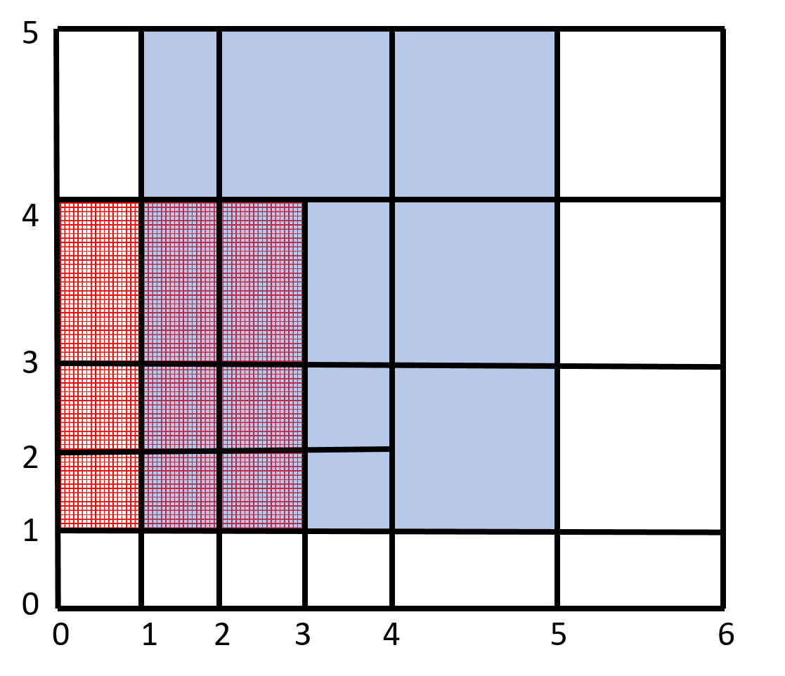
Figure 3: Parameter domain of an LR B-spline surface with indication on B-spline support. The knot line segments are shown as black lines. The support of two overlapping B-splines are shown in red and in blue

The incremental refinement by knot insertion used by Locally Refined B-splines ensures that the splines spaces generated are nested. Figure 3 shows a parameter domain and the segmentation into boxes corresponding to a bi-quadratic LR B-spline surface. In addition the support of two tensor product B-splines is shown. We see that a knot line segment stops inside the blue tensor product B-spline support. This knot line is excluded from the local knot vectors defining the tensor product B-spline covering this support.

3.3.3 Notation and summary

To simplify notation will from now on use the scaled tensor product B-splines defined in Equation 5. An LR B-spline surface of bi-degree $(p_{1},p_{2})$ is given as

$$F(u,v)=\sum_{B\in\mathcal{B}_{j}}c_{B}N_{B}(u,v).$$ (8)

The scaled tensor product B-splines used for describing an LR B-spline surface are non-negative by construction and has a compact support with size depending on the knot configuration. Partition of unity is obtained as described in Equation 5. In many situations $s_{B}\equiv 1$, but occasionally when more tensor product B-splines than $(p_{1}+1)(p_{2}+1)$ overlap an element, then $0<s_{B}<1$, for some of the B-splines.

It is practical to store all knot values used in global knot vectors to allow indexing of knot values as in done in the representation of locally refined splines in Part 42 of ISO 10030 (STEP). $\mathbf{u}_{G}=\{u_{0},u_{1},\ldots,u_{N_{1}+p_{1}}\}$ and $\mathbf{v}_{G}=\{v_{0},v_{1},\ldots,v_{N_{2}+p_{2}}\}$ as in the tensor product case.

Linear independence of the resulting collection $\mathcal{B}_{j}$ of LR B-splines is not guaranteed in general, but is ensured for the constructions used in this article. Violations to the linear independence can be detected and resolved by dedicated knot line insertions. Linear dependence of LR B-splines is addressed in detail in Patrizi-2020 .

4 Surface formats for terrain and sea bed

Table 1: Summary of surface formats for representing terrain and sea bed.

	Representation and data structure	Algorithm and control of accuracy	Surface smoothness	Restricting data volume
Raster	Values on regular mesh.	Spatial interpolation to define sample values. Accuracy checked after creation.	Depends on interpolation method for evaluation between mesh points.	Pre-set mesh resolution defining data volume.
Tensor product B-spline surface	Piecewise polynomials on regular mesh, any bi-degree.	Coefficients calculated by local/global approximation. Accuracy checked after surface creation.	Depends on polynomial degree.	Pre-set mesh resolution defining data volume.
TIN	Triangulation.	Triangulate point cloud + thinning or adaptive triangulation. Accuracy can be checked during creation.	$C^{0}$	Pre-set approximation tolerance and/or max allowed data volume.
LR B-spline surface	Piecewise polynomial on locally refined axes parallel mesh, any bi-degree.	Coefficients calculate by local/global approximation. Local adaption by checking accuracy during construction and refinement where needed.	Depend on polynomial degrees.	Pre-set approximation tolerance or restrictions in adaptive algorithm.

Table 1 provides an overview over the surface representations discussed in the Sections 2 and 3. TIN and LR B-spline surfaces are created by adaptive algorithms, the algorithm for LR B-spline surfaces are presented in Section 5. Thus, degrees of freedom in the surface can be defined according to needs, and the accuracy of the fit can be made directly available. The raster representation and the tensor product (TP) B-spline surfaces are less flexible although adaptive refinement can be applied to TP-surfaces as well. The lack of local refinement, however, imply that the TP-surface size grows much faster than in the LR B-spline case. The spline methods provide smoother surfaces than the alternatives.

Tensor product B-spline surfaces can be regarded as a generalization of the raster representation. A regular grid of polynomial elements describes the surface instead of the regular grid of points in a raster representation. In contrast to the raster representation the tensor product surface is uniquely defined by its representation. Point and derivative evaluation in the entire surface domain is performed without ambiguity. Furthermore, the tensor product surface description is more flexible than the raster due to the choice of polynomial degrees, variable distances between consecutive knots and the possibility of defining the surface in a geometry space with dimension higher than one. Due to the low flexibility the raster representation is more compact than using a tensor product B-spline surface for the representation of a piecewise constant function.

LR B-spline surfaces provides local refinement of tensor product B-spline surfaces and the raster representation used in GIS. The flexibility is still lower than the case for TIN, but it is a smooth representation that avoids the ragged appearance that can occur for TIN. The LR B-spline format can represent the smooth component of terrain and sea bed more effectively than a triangulation. Whether LR B-spline surfaces or TIN is the most appropriate representation will depend on the characteristics of the data and the purpose of the surface generation.

5 Scattered data approximation with LR B-spline surfaces

Data: Point cloud, maximum number of iterations, threshold

Result: Approximating surface, information on approximation accuracy

Generate initial surface;

Compute accuracy;

while there exists points with larger distance than the given threshold and the maximum number of iterations is not reached do

       Refine the surface in areas where the tolerance threshold is not reached;

       Perform approximation in the current spline space;

       Compute accuracy;

      

end while

Algorithm 1 Iterative algorithm for LR B-spline surface generation

Approximation of a point cloud with an LR B-spline surface is performed in the iterative process presented in Algorithm 1 and described in some detail in lralg1 and lralg2 . We will here provide a summary. The accuracy of a current approximating surface is a measure on the distance between the point cloud and the surface in the height direction. The maximum distance, the average distance and the number of points, where the distance is larger than the given threshold, is computed at every iteration step and used to decide where the surface needs to be refined.

In this paper we let the x- and y-coordinates of the points serve as the parameter values while the surface (or function) approximates the z-component of the data, but the algorithm handles parameterized points as well (each point is given with a parameter pair and 3D coordinates). We will, in the following, focus on elevation and therefore change the notation of the surface parameters from $u$ and $v$ to $x$ and $y$.

Initially, the point cloud is approximated by a tensor product spline surface. A tensor product B-spline surface is a special case of an LR B-spline surface and this initial surface is represented as an LR B-spline surface to start the iteration. The distances between the surface and the points are computed in every point, and the derived accuracy information is distributed to the polynomial elements of the surface. As long as the maximum distance between the points in an element and the surface is not below the given threshold, the element is a candidate for splitting. A broad discussion on strategies for refinement can be found in refineLR . A new knot line segment must completely traverse the support of at least one B-spline as explained in Section 3.3.2. One new segment will increase the number of coefficients in the surface with at least one. To take advantage of the new degrees of freedom the surface is updated either by a least squares approximation or by applying the multi-level B-spline algorithm (MBA) mba . These steps are repeated until either the maximum distance between the surface and the point cloud is less than the given threshold or the maximum number of iteration steps is reached.

A geospatial point cloud may represent a very rough terrain and contain noise and possible outliers. Thus, it is not necessarily beneficial to continue the iterations until all points are closer to the surface than the threshold. Typically, the process is stopped by the number of iterations. In refineLR it is shown that the accuracy improvement tends to drastically slow down when most points have a distance to the surface less than the threshold. Recognized outlier points may be removed during the iterative approximation process, but distinguishing between features and outliers is not a simple task. The topic is not pursued in this paper.

Least squares approximation is a global method where the following expression is minimized with respect to the surface coefficients ${c_{B}}$ over the entire surface domain:

$$\min_{\mathbf{c}}[\alpha_{1}J(F(x,y)+\alpha_{2}\sum_{k=1}^{K}(F(x_{k},y_{k})-z_{k})^{2}].$$

$F(x,y)$ is the current LR B-spline surface, see also Equation 8, and ${\mathbf{x}}=(x_{k},y_{k},z_{k}),k=1,\ldots,K$ are the data points. The expression is differentiated and turned into a linear, sparse equation system in the number of surface coefficients. A pure least squares approximation method will result in a singular equation system if there exists B-splines with no data points in its support. As an LR B-spline surface is defined on a rectangular domain and a typical point cloud has a non-rectangular outline and may contain holes, parts of the surface domain will frequently lie outside the domain of the point cloud. $J(F(x,y)$ is a smoothness term that enables a non-singular equation system even if this situation occurs. In our case the smoothness term is an approximation to the minimization of curvature and variation of curvature in the surface. These originally intrinsic measures are made parameter dependent to give rise to a linear equation system after differentiation. The smoothness term is expressed as

$$J(F(x,y))=\int\int_{\Omega}\int_{0}^{\pi}\sum_{i=2}^{3}w_{i}\Big{(}\frac{\partial^{i}F(x_{0}+r\cos\phi,y_{0}+r\sin\phi)}{\partial r^{i}}\Big{|}_{r=0}\Big{)}\mathrm{d}\phi\mathrm{d}x_{0}\mathrm{d}y_{0}.$$

At each point $(x_{0},y_{0})$ in the surface domain, $\Omega$, a weighted sum of the directional first and second derivatives of the surface is integrated around the circle and the result is integrated over the surface domain. The directional derivative is represented by the polar coordinates $\phi$ and $r$.The two terms in $J(F(x,y)$ are given equal weight. A more detailed description can be found in smooth1 . The weight on the smoothness term is kept low to emphasize the approximation accuracy. In the examples of the next sections $\alpha_{1}=1.0\times 10^{-9}$ and $\alpha_{2}=1-\alpha_{1}$. A suite of other smoothness terms is presented in smooth2 .

Multi-level B-spline approximation (MBA) is a local, iterative approximation method, see mba . The coefficients $q_{T}$ of the residual surface are computed individually for each scaled tensor product B-spline $N_{T}$. They are determined from the collection of data points $P=(x_{P},y_{P},z_{P})\in\mathcal{P}_{T}$ in the support of $N_{T}$ as well as the magnitude of the residuals, $r_{P}=z_{P}-F(x_{P},y_{P}),P\in\mathcal{P}_{T}$.

$$q_{T}=\frac{\sum_{P\in\mathcal{P}_{T}}N_{T}(x_{P},y_{P})^{2}\phi_{T,P}}{\sum_{P\in\mathcal{P}_{T}}N_{T}(x_{P},y_{P})^{2}},$$ (9)

where $\phi_{T,P}$, addressed below, depends both on the residuals of the points in $\mathcal{P}_{T}$ and the collection of B-splines $\mathcal{B}_{T}$ with a support overlapping at least one point in $\mathcal{P}_{T}$. For each of the residuals we define an under-determined equation system

$$r_{P}=\sum_{B\in\mathcal{B_{T}}}\phi_{B,P}N_{B}(x_{P},y_{P}),P\in\mathcal{P}_{T}.$$

where $\phi_{B,P}$ are unknowns to be determined. There are many solutions of this equation system. For MBA the choice is

$$\phi_{B,P}=\frac{N_{B}(x_{P},y_{P})r_{P}}{\sum_{B^{\prime}\in\mathcal{B_{T}}}N_{B^{\prime}}(x_{P},y_{P})^{2}},\,{B\in\mathcal{B}_{T},P\in\mathcal{P}_{T}}.$$

Now we select $\phi_{T,P},P\in\mathcal{P}_{T}$ to add the missing piece in Equation 9. The process is explained in more detail in mba2 .

The updated surface is the sum of the last surface and the obtained residual surface. MBA is an iterative process and repeated applications of the algorithm converge towards the best approximation of the point cloud given a collection of B-splines. In the examples following MBA will be run twice for each step in the approximation algorithm.

In lralg1 the two approximation algorithms are compared in a number of examples. In general, the least squares algorithm has a better approximation order while the MBA-algorithm is more stable when the spline space is less regular and/or the number of points in each element is low. Typically, we use least squares approximation in the first few iteration steps, then turn to MBA.

5.1 Example: Approximating a geospatial point cloud by an LR B-spline surface

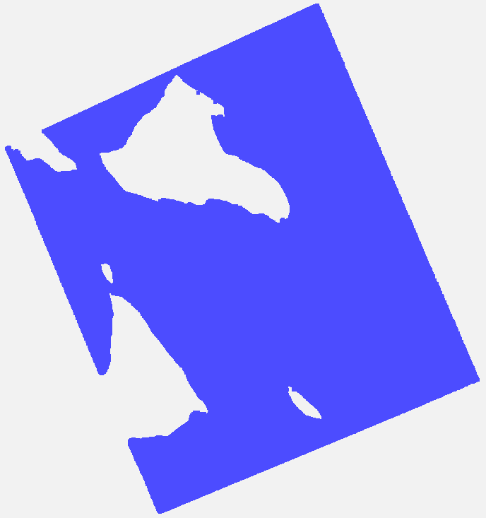
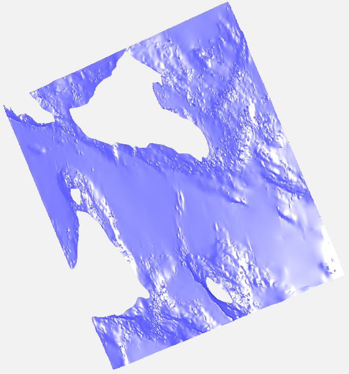
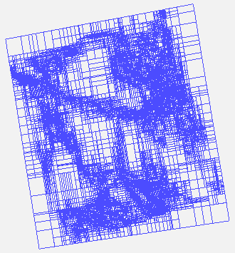
(a)	(b)	(c)

Figure 4: (a) Outline of point cloud, (b) LR B-spline surface, (c) the element structure of the surface

We will illustrate the LR B-spline approximation framework by applying the algorithm to a selected data set. The same data set and corresponding surface will be used to explain how the locally refined spline approach can be used in a GIS work flow, and how the approximation algorithm can be tweaked to further utilize the flexibility of the LR B-spline format. Consider Fig. 4. The data set Fig. 4(a) covers an area of slightly less than one square kilometer close to the Norwegian coast. It consists of about 11 millions points with a quite uniform density although some holes. The area is shallow, the depth varies from -27.94 meters to -0.55 meters. The point cloud contains outliers. The theoretical least maximum distance between the surface and the point cloud is 1.19 meters as the cloud contains one pair of points with the same $(x,y)$-coordinates and different depths. A surface created with 7 iterations in Algorithm 1 and a threshold of 0.5 meters is shown in Fig. 4(b). The data set is not compliant with a rectangular area and contains holes while an LR B-spline surface is defined on a rectangular domain. The valid part of the surface corresponding to this data set is defined by the use of trimming. The surface is bi-quadratic. This choice results in a smooth surface with the flexibility to represent data sets with local depth variations. The choice of polynomial degree is investigated in refineLR . The sea floor covered by the data set contains both smooth areas and areas with significant variation. This can be recognized by the element structure of the surface shown in Fig. 4(c). We can also see that the surface is less refined in areas where there are no points.

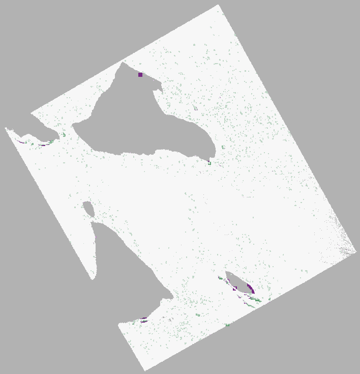
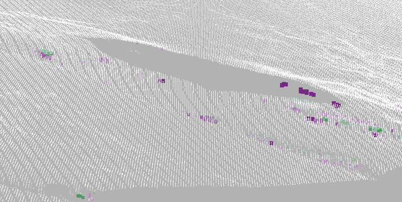
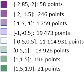
(a)	(b)

Figure 5: (a) The point cloud coloured according to the distance to the LR B-spline surface. (b) A detail and colour scale.

The surface has 33 830 coefficients and fits 99.68% of the points within the threshold. The average distance between the point cloud and the surface is 0.068 meters and the maximum distance is 2.85 meters. In Fig. 5(a) the point cloud is coloured according to the distance to the surface. Fig 5(b) shows a detail of the same point cloud along with the colour scale and the distance distribution of the points. Points that are distant to the surface are magnified compared to closer points. The point with the maximum distance to the surface belongs to the group of points in Fig. 5(c) that is slightly separated from the rest of the point cloud.

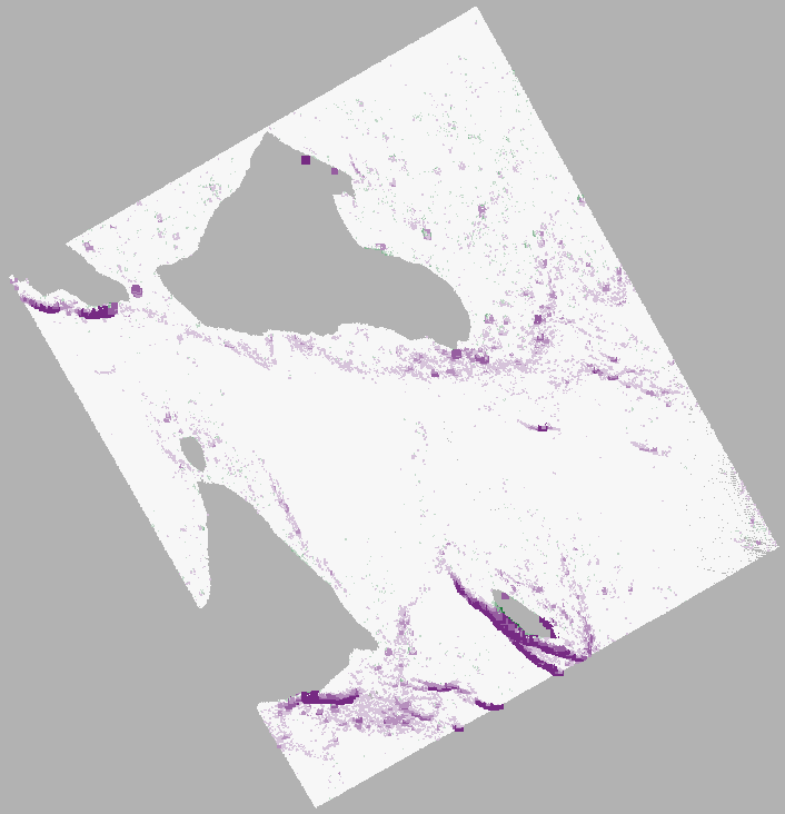
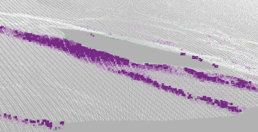
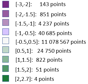
(a)	(b)

Figure 6: (a) The point cloud coloured according to the distance to the raster with resolution 2 meters. (b) A detail.

The LR B-spline surface in Fig. 4 is more refined in rough than in smooth areas, but there are still more points with a large distance to the surface in the rough areas. This effect is expected to be more dominant in a raster representation. Fig. 6(a) shows a set of points estimated from a $443\times 492$ raster representation of the initial data set. The raster has resolution 2 meters in both parameter directions and is computed with IDW. The points displayed have the same $(x,y)$-parameters as the initial data points and the depths are estimated by evaluating a bi-linear patch interpolating the nearby sample points. The points are coloured according to the distances to the initial points and the colour coding and distance distribution is shown in Fig. 6(b) along with a detail covering the same area as in Fig. 5(b). The maximum distance is 4 meters and the average distance is 0.12 meters. The points with low accuracy are focused in steep and ragged areas of the sea bed.

The applied inverse distance weighing interpolation uses a limited but high number of points to estimate the sampling points with a radius, $R$, specifying the area in which points used in the computation is collected. We set $R$ equal to 20 meters. The value $z$ of the sampling point $\mathbf{x}=(x,y)$ is given by

$$z(\mathbf{x})=\frac{\sum_{i=1}^{N}w_{i}(\mathbf{x})z_{i}}{\sum_{i=1}^{N}z_{i}},$$

where $z_{i}$, $i=1,\ldots,N$ are the elevation values of the data points used to estimate the current sampling point. The weight is computed as

$$w_{k}(\mathbf{x})=\Big{(}\frac{\max(0,R-|\mathbf{x}-\mathbf{x_{k}}|)}{R|\mathbf{x}-\mathbf{x_{k}}|}\Big{)}^{2}.$$

Here $\mathbf{x_{k}}=(x_{k},y_{k})$ is the position corresponding to elevation value $z_{k}$.

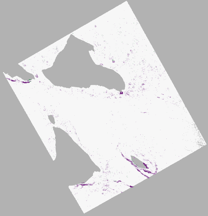
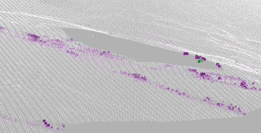
(a)	(b)

Figure 7: (a) The point cloud coloured according to the distance to the raster with resolution 0.5 meters. (b) A detail.

The accuracy of a raster with resolution 0.5 meters is shown in Fig. 7. The raster size is $1\,769\times 1\,967$, the maximum distance between the point cloud and the raster surface is 2.96 meters and the average distance is 0.068 meters. The accuracy is improved compared to the lower resolution raster, but the distances between the surface and the point cloud are still larger than for the LR B-spline surface. The largest distances are still to be found in steep and ragged areas. The IDW interpolation method and the bi-linear estimation of points in the surface are chosen for simplicity. Other interpolation approaches may result in better accuracy, but the effects of the raster representation remain.

The raster surfaces are represented as GeoTIFF files with sizes 852KB and 14MB for the raster with resolution 2 meters and 0.5 meters, respectively. The size of the LR B-spline surface is 2.5MB. GeoTIFF is a binary format where the height values are stored as float, while the LR B-spline surface is stored in an ASCII file using doubles for the storage of coefficients. The height values of the raster with 2 meters resolution sum up to 217 956 floats. The storage of the LR B-spline surface requires a total of 537 175 numbers, of which 35 801 are doubles and the remaining are integers. A compressed version of the LR B-spline file has a size of 584KB.

Can more iterations in the approximation algorithm improve the accuracy of the LR B-spline surface further? Increasing the number of iterations to 9, the number of points with a distance larger then 0.5 meters decreases to 21 446 while the number of coefficients grows to 203 772 and the file size increases from 2.5MB to 16MB. The file size of the point cloud is 359MB. After 16 iterations the least possible maximum distance of 1.19 meters is reached. The average distance is 0.052 meters and 476 points are further away from the surface than the given threshold. The surface size has grown 53MB. Continuing to 20 iterations another 5 points are within the threshold at the cost of increasing the surface size with 4MB. It is not necessarily a gain in insisting on the maximum possible accuracy. Accuracy must be balanced against the surface size and approximation of noise and outliers is not attractive.

6 Export

The LR B-spline representation format is relatively new, and the current support is limited. Thus, an option to export these surfaces to other formats is crucial for the use of the LR B-spline format. Raster is the standard representation for terrains and sea bed, and raster creation is a matter of regular evaluation, possibly with some adaption to features such as extremal points, ridges and valleys. A raster representation will, in general, not support the same level of detail as an LR B-spline representation of an area, but a high accuracy LR B-spline surface can give rise to rasters of different resolution. Thus, the LR B-spline surface can serve as a master representation to be harvested according to needs.

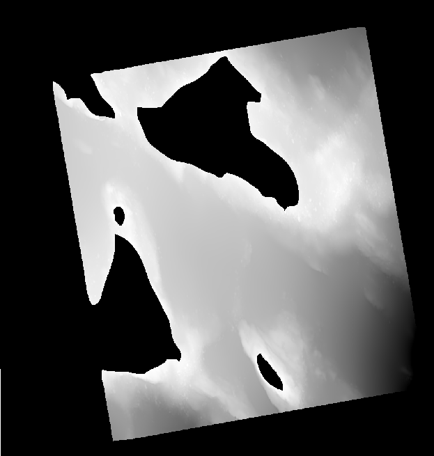
(a)	(b)	(c)

Figure 8: (a) Raster with one meter resolution. (b) A detail. (c) Detail with five meters resolution

Fig. 8 shows raster representation at two different resolutions generated from the LR B-spline surface in Fig. 4.

6.1 Export as ISO 10303 LR B-spline surfaces

ISO 10303 (STEP) is a standard for digital exchange of product data. It has a broad scope, but CAD data exchange was an early adapter of the standard. Tensor product spline surfaces belong to the generic resources (Part 42) and in the context of the EC Factories of the Future project TERRIFIC (2011-2014), it was proposed to extend Part 42 with locally refined surfaces. The extension was published as part of STEP in 2018. It is ongoing work to make this format available for STEP users. In the future LR B-spline surfaces can be exchanged directly through STEP.

6.2 Export as tensor product B-spline surfaces

Direct export of LR B-spline surfaces through neutral exchange formats is an option in the future. Being a spline surface, an LR B-spline surface can be expanded to a tensor product (TP) spline surface at the cost of a potentially large increase in data size. This conversion contradicts the idea of locally refined splines. The size of the surface in Fig. 4 would increase from 2.5MB to 17MB and the increase in the number of polynomial elements is much higher due to different file formats. An LR B-spline surface could be exported as a set of Bezier surfaces, but as such a surface typically contains a high number of polynomial elements, it is not obvious that this is a good solution. A better option is to represent the LR B-spline surface by a collection of tensor product spline surfaces maintaining the feature of data size distributed according to needs.

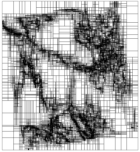
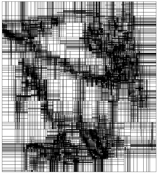
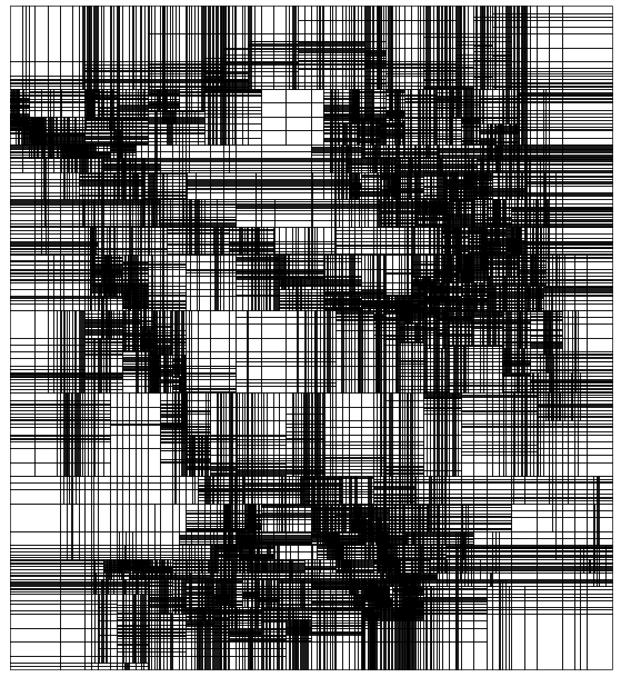
(a)	(b)	(c)

Figure 9: (a) LR B-spline surface mesh. (b) Mesh when the surface is divided into 666 TP surfaces. (c) Mesh when the surface is divided into 300 TP surfaces

Fig. 9 indicates how the LR B-spline surface shown in Fig. 4 can be divided into tensor product spline surfaces by the means of dedicated knot line insertions. Image (a) shows the polynomial patches of the LR B-spline surface, (b) and (c) shows the patches after dividing the surface into 666 and 300 tensor product patches, respectively.

The division into TP surfaces is performed by a recursive algorithm. At each level it considers how the current surface can be split by extending one knot line to cover the entire surface domain. The candidate knot line must contain T-joints, that is at least one knot line in the other parameter direction must end at this knot line. The number of surface elements overlapping the knot line extension should be minimized and at the same time the knot line should divide the current surface into two surfaces with roughly the same number of knots. The balance between the two criteria varies throughout the recursion levels. When an appropriate split is found, the algorithm proceeds to look for splits in the two sub surfaces. The splitting algorithm stops when no sub surface contains more segmented knot lines than a given threshold. Each sub surface is expanded to a tensor product spline surface by adding missing knot segments.

7 Analysis Tools

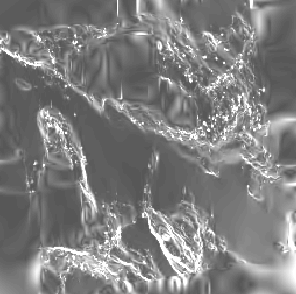
Figure 10: The slope of the surface in Fig. 4 (b) is evaluated in a raster

A GIS surface can be used to gain insight in the domain it represents. Along with visualization, properties such as slope, aspect and contour curves are computed. Being a spline surface a point-wise computation of slope and aspect is a straight forward task, an example of slope is shown in Fig. 10. We will here go into some details regarding contour lines and also present computation of minimum and maximum points.

7.1 Contour lines

Calculation of contour curves is supported in GIS systems. LR B-spline surfaces representing elevation are piecewise polynomial functions, and contour curves are curves where the value of the spline function is constant. We want to find $f_{a}(t)=(f_{1}(t),f_{2}(t))^{T}\in R^{2}$ such that $F(f_{1}(t),f_{2}(t))=a$ for an LR B-spline surface $F$ and an of elevation value $a$.

Instead of developing interrogation functionality for LR B-spline surfaces, we split the LR B-spline surface into a number of tensor product surfaces as described in the previous section. Then we use the interrogation functionality of SINTEF’s spline library, SISL sisl on each sub surface.

Fig. 11 (a) shows how the example surface in Section 5.1 is split into TP surfaces while (b) shows contour curves with one meter resolution. The contouring problem corresponds to computation of intersections between a parametric spline surface and an algebraic surface, a problem that is discussed in intersect2 . The applied algorithm contains several phases:

1. Divide the LR B-spline surface into a set of TP surfaces

2. For each value $a$ and each TP surface

   1. Compute the topology of the contour curves using SISL. This is a recursive algorithm that finds a set of “guide points” on each curve branch.

   2. Trace each identified curve branch starting from an identified “guide point”. Represent the curves traced out as spline curves.

3. For each value $a$: combine sub curves from different TP-surfaces into contour curves for the entire LR B-spline surface.

The contour curves will be accurate with respect to the given elevation values and approximate the LR B-spline surface with respect to a given tolerance.

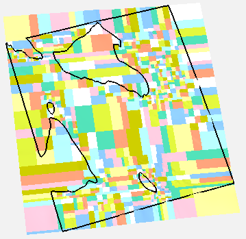
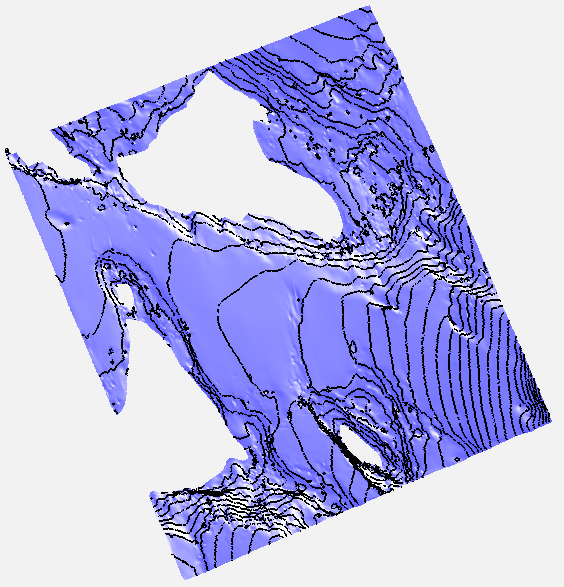
(a)	(b)

Figure 11: (a) Division into TP surfaces. The trimming loops corresponding to the LR B-spline surface are shown in black. (b) Surface with contours, one meter resolution

An LR B-spline surface approximating an area with large shape variation will contain many details, which again will lead to a complex pattern of contour curves, see Fig. 12 (a). The tensor product surfaces are distinguished by colour, and we will describe the computation of a set of contour curves on the central TP surface in some detail.

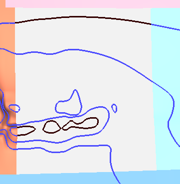
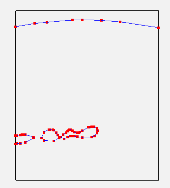
(a)	(b)

Figure 12: (a) Contour curves detail. (b) Result from the topology detection phase of computing the black contour curve in (a). Connected guide points describes 4 contour curves

The surface patch is in very shallow water and contains contour curves at the depths of two, three and four meters. The pattern of contour curves at depth two meter (black curves in Fig. 12(a)) is complex with one curve passing between opposite boundaries, one curve with both endpoints at the left boundary and two very dense inner closed loops. The topology detection is concerned with identifying this pattern and generating starting points for the proceeding tracing of the contour curves. Also guide points that give a more complete description of the curves are computed. The algorithm uses a recursive approach:

1. Check if there is any possibility that the elevation value $a$ is in the range of the the current function. Otherwise, stop the computation.

2. Compute all intersection points at the surface boundaries. This is done recursively in the number of parameter directions. The structure of the lower dimensional algorithm follows the pattern of the algorithm described here.

3. Check if there is any possibility that the elevation value is in the range of the function excluding boundaries. If not stop the computation at this recursion level.

4. Check for a possible existence of inner closed intersection loops. If not mark connections between intersection points at the boundaries and stop the computation at the current recursion level.

5. Divide the surface into two or four.

6. Compute intersections between the given elevation value and the boundaries between sub surfaces.

7. For each sub surface go to 3

More details can be found in recursive . Efficiency and robustness of the algorithm is reached through good interception methods and a clever strategy for dividing the surface into sub surfaces. A discussion on subdivision strategies for surface intersections can be found in intersect . A general rule is to subdivide at singularities and internal in closed loops. A complex situation lead to more subdivisions and consequently more guide points as shown in Fig. 12 (b). The relatively simple curve at the top is identified with fewer subdivisions.

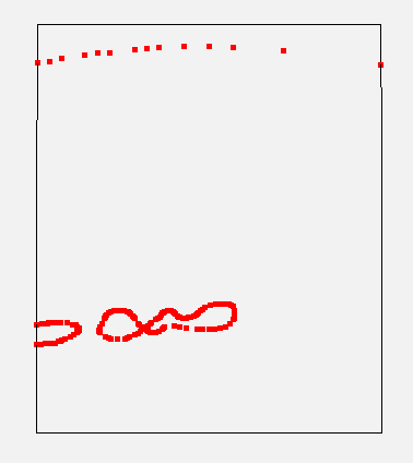
Figure 13: Tracing the result from guide points.

Consider again the current TP surface in Fig. 12 and denote the surface $\tilde{F}(u,v)$. The surfaces is bi-quadratic and $C^{1}$ continuous. This degree of smoothness imply that the contour curves can turn quite sharply at knot lines. The objective when tracing a contour curve is to describe the curve with sufficiently accuracy, handle sharp turns in the curve and avoid jumping to a different contour curve. In the current case, the distance between the two closed loops is very small. The algorithm works as follows: For a current point $(u_{0},v_{0})$ on the contour curve estimate the position of the next point and iterate it onto a contour curve. The contour curve tangent direction at the point is, in the parameter domain, given by $(-\frac{\partial F}{\partial v}(u_{0},v_{0}),\frac{\partial F}{\partial u}(u_{0},v_{0}))$ and the step length is deduced from the lengths of the first and second surface derivatives at the point and the surface size. Ensure consistency of the directions between the start point and the endpoint of the current segment, and between both points and the midpoint of the segment. Other intermediate points may also be involved in the verification of consistency. If consistency is not verified, a new candidate endpoint closer to the current one is computed and the process is repeated. The tracing function uses information about the first and last guide point obtained from the topology detector and whether or not the curve is closed. Typically, the tracing function will produce a denser and more uniform sequence of points than the topology detector, see Fig. 13. A simple configuration leads to less points than a more complex one.

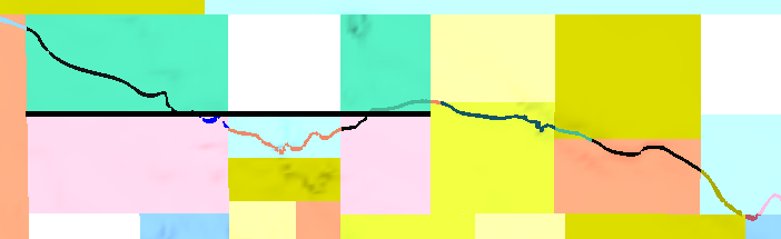
Figure 14: Joining curve fragments into complete contour curves across TP surface boundaries. Detail. The various curve segments have different colours and TP surfaces are also distinguished by colour.

The final step is, for each elevation value $a$, to join curve segments across the boundaries of the tensor product surfaces, see Fig. 14. Here two pairs of curve segments belonging to an open curve need to be merged at the surface interface marked with a horizontal black line. Note that there are still curve segments that need to be merged in the other parameter direction. During the processing of the interfaces between the TP surfaces, more and more small curve fragments will be joined and finally all contour curves will end at boundary curves of the complete LR B-spline surface, they will be closed or meet at a branch point in the inner of the surface.

7.2 Extremal points

Information about minimum and maximum points (extremal points) can contribute to get a picture of the behaviour of the terrain or sea bed in a given area. Such points are also contained in the set of standard map information, provide important information in the computation of a lower resolution representation of the domain, and are candidates for landmarks. However, it is not obvious how these points should be defined. The partial surface derivatives at an extremal point are zero and a maximum point has the least depth in the vicinity. Similarly, is a minimum point situated at the locally greatest depth. This rules out saddle points that typically will be placed between two extremal points of the same type. Consider the surface visualized in Fig. 4 (b) and Fig. 11 (b). This surface probably has one or a few global maxima, mostly placed at surface boundaries and also a few global minima. The surface has a huge amount of local extrema and the higher the accuracy of the approximation, the higher is the expected number of local extrema.

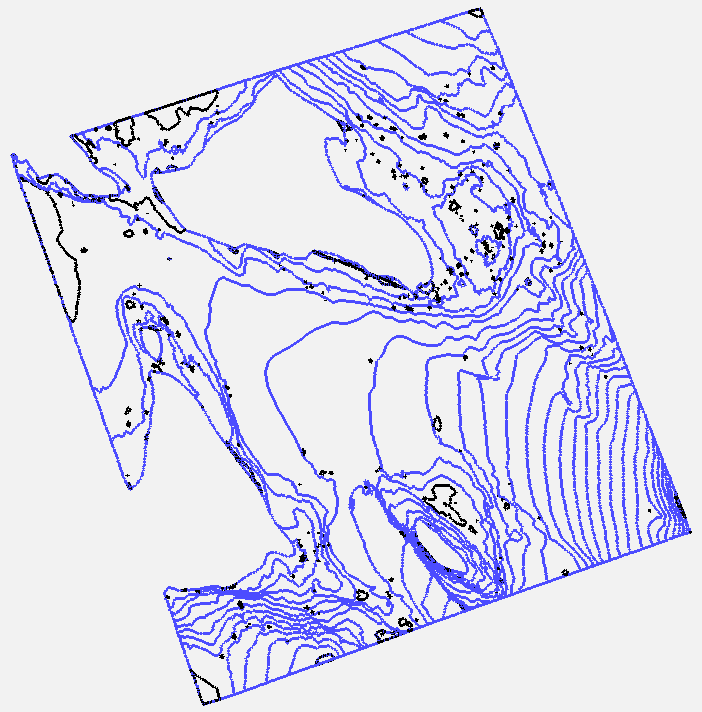
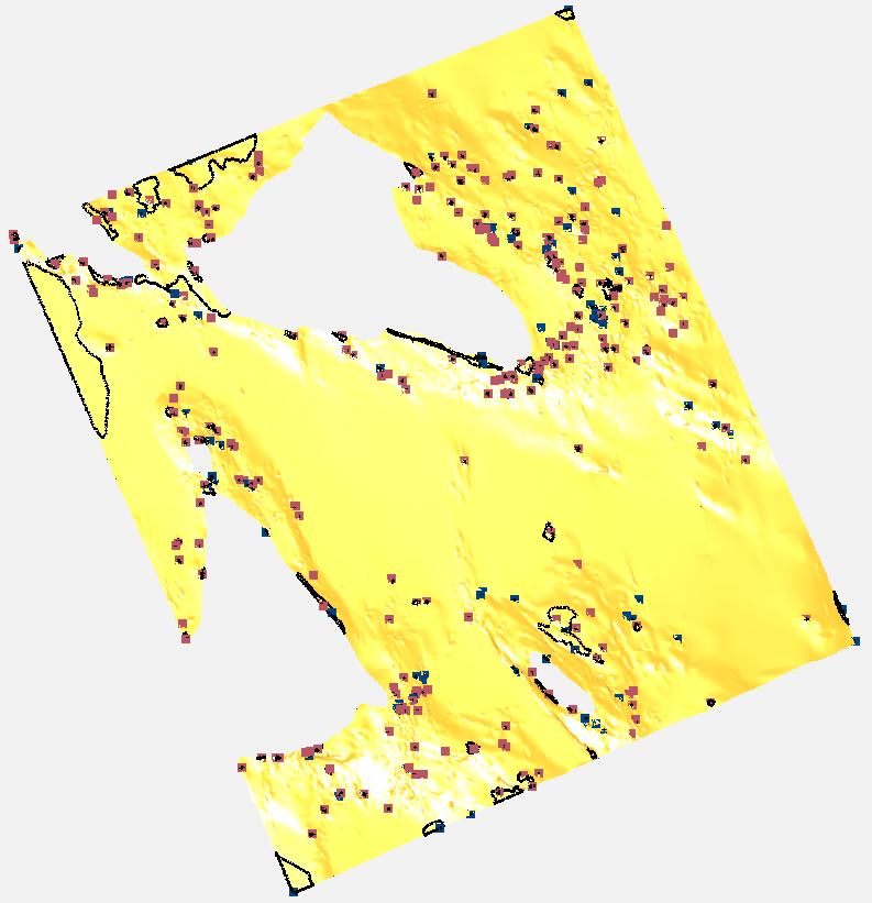
(a)	(b)

Figure 15: (a) Contour loops. The black curves trigger the computation of extremal points. (b) The surface with trigger curves and identified extremal points.

The granularity of the extremal point definition can be linked to the granularity of the contour curves. Minimum and maximum points that do not deviate more from their surroundings than the interval between subsequent elevation values are not regarded as significant. Thus, a condition for the existence of an extremal point in an area is that the extremal point is surrounded by a closed contour curve or a contour curve meeting the surface boundaries. Furthermore, there must be no contour curves inside an identified one that are associated with the same type of extremal point. If the terrain height increases through a contour curve, before decreasing again to form a dump, it can be appropriate to define both a minimum and a maximum point. Fig. 15 (a) shows the contour curves of the test surface. The ones indicating an extremal point are black. In (b) the calculated extremal points are shown together with the surface and the trigger curves. We see that the vast majority of extremal points are maximal and that they are quite densely distributed in some areas. Typically, the surface has local height variation in the vicinity of a contour level, which can give extremal points of low significance. Thus, post processing of the found extremal points will be needed to get a more representative selection.

Each trigger curve defines an area in which one minimum or maximum point is to be found. This area is represented as trimmed tensor product surfaces using a similar approach as in the computation of contour curves. Normally, one area leads to one TP surface. One global extremal point is computed for each TP surface. The strategy is very similar to the topology detection functionality for contour curves. Extremal points at the surface boundaries are identified. A check for a possibly more extreme point in the inner of the surface is performed. Since the surface is bounded by its coefficients the maximum value of the surface will be restricted by the maximum coefficient. If the control polygon given by the surface coefficients changes direction at most once in a parameter direction, then there will be at most one extremal point in the surface, and an iteration for the local extreme can be performed. Previously found, less extreme, points are removed when a new extremal point is identified. If the current surface is too complex to conclude with a result, the surface is subdivided and the search continues on each sub surface.

The search for a global extremal point is performed on the local, non-trimmed tensor product surface. Thus, it is necessary to check whether the found point is actually inside the trimmed surface. The terrain configuration combined with knowledge of an existing extremal point indicates that this point often will lie in the trimmed surface. However, in areas with dense extremal points, the algorithm may identify another extreme point lying within the non-trimmed TP surface. In our test case 52 out of 460 found extremal points situated outside the trimmed surface. A fallback strategy is required to identify the extremal point inside the trimming loop. A number of sample points provide start points for an extremal point iteration. Then the most extreme point is selected.

8 Adopting the approximation to emphasize particular areas

In shallow waters, as is the case in our example, an accuracy of the surface representation of in essence 0.5 meters may not be sufficient. In particular the boat traffic may need more exact information about shallows. We will, in this section, investigate some strategies for ensuring sufficient clearance in critical areas. Table 2 summarizes the experiment setups investigated in this section. The setup codes are constructed as follows: F means approximation with a fixed threshold and V with a variable threshold; S means that significant points are included in the computation; E indicates that a minimum element size is defined; WM stands for the weighted mid surface; The first digit represents the maximum number of iterations and the second, when given, the minimum element size. Variable threshold and a restriction to the element size of the surface is treated in Section 8.1, the weighted mid surface in Section 8.2 and significant points in Section 8.3.

Table 2: Parameter settings for surface approximation. The threshold is given in meters, the number of iterations varies between seven and nine.

Setup	Threshold	No iter	Comment
F7	0.5	7	Example of Section 5.1
V7	0.20022 - 0.31176	7	Variable threshold
V9	0.20022 - 0.31176	9	Variable threshold
V9E1	0.20022 - 0.31176	9	Restricting the element size to 1 $\times$ 1 square m.
V9E2	0.20022 - 0.31176	9	Restricting the element size to 2 $\times$ 2 square m.
WM7	0.5	7	Weighted mid surface
FS7	0.5	7	266 significant points, threshold 0.2 meters
FS9	0.5	9	266 significant points, threshold 0.2 meters

8.1 Surface approximation with a depth dependent threshold

The specified accuracy threshold influences the approximation process in two ways: It governs where the surface is refined; and, decides when the distance between the surface and the point cloud is sufficiently small. At each iteration step, the point cloud will be approximated as accurately as allowed by the spline space. A tighter threshold leads to more accurate surfaces, but it also increases the surface size.

The concept of local refinement allows more degrees of freedom in the surface where the point cloud has local details. A variable threshold can lead to a more accurate surface fitting in critical areas and focus on representing the smooth component of the data in areas where the accuracy is less critical. We now let the threshold depend on the sea depth at each point. Shallow water lead to a stricter tolerance than great oceans depths.

Table 3: Figures of accuracy for approximations with varying number of iterations and accuracy thresholds. The total number of points is 11 150 110 and the size of the data file is 297 MB. For each parameter setup the sizes of the approximating surface in MB are reported along with the number of surface coefficients and the maximum and average distances between the point set and the surface. The number of points having a distance to the surface of less than 0.2 meters, between 0.2 and 0.5 meters and more then 0.5 meters are given in column 6, 7 and 8, respectively. The different setups are specified in Table 2.

Setup	Sf. size	No. coefs.	Max dist.	Av. dist.	$<$ 0.2	$<$ 0.5	$\geq$ 0.5
F7	2.5MB	33 830	2.85 m.	0.068 m.	10 429 550	685 381	35 179
V7	16MB	206 295	2.81 m.	0.052 m.	10 753 948	336 828	27 334
V9	139MB	1 853 313	2.48 m.	0.042 m.	10 957 497	179 908	12 705
V9E1	9.6MB	139 754	2.81 m.	0.055 m.	10 730 787	388 785	30 538
V9E2	3.7MB	53 824	2.82 m.	0.063 m.	10 496 438	609 920	43 752

Table 3 compares the obtained surface approximation accuracy for different refinement requirements. Setup F7 corresponds to the surface in Fig. 5. 0.32% of the points lie outside the given threshold of 0.5 meters. For the remaining cases having a varying threshold, the percentage of points with a distance larger than the threshold is 2.68%, 1.37%, 3.12% and 4.98%, respectively. The data size increases significantly with a stricter threshold and more iterations applied in the approximation algorithm. The element size of the final surface may in some areas be in the magnitude of the point cloud resolution. To avoid approximation of noise or irrelevant details a restriction on the element size can be applied. This limits the surface size, but influences also the approximation accuracy as can be seen in Table 3, Setup V9E1 and V9E2.

The accuracy improves when the number of surface coefficients increases, but at a slower pace. The average distance between the surface and the points is always kept low as the surface approximates smooth data very well. The larger distances are caused by a non-smooth behaviour in the data that can be due to variation in the sea bed like stones, small inconsistencies in the data set or even outliers, which is present in this data set. In fact, the surface tends to emphasize too much on such variation if the degrees of freedom are high as can be seen in Fig. 16 where the surface with the highest number of coefficients (a) and (b) is very detailed in some areas. The less detailed surface in (c) also captures the main behaviour of the sea bed, but omits some details. The approximation setup must reflect the data set properties and in this case the point cloud contains noise. Although being variable the provided threshold is strict and lead to a high number of coefficients. A depth dependent tolerance threshold is better suited to impose a less detailed approximation at large depths.

The threshold and the maximum number of iteration steps is important for the approximation result. Currently these parameters are set manually, but there is ongoing research to find a process related stop criteria for the iteration and to set the threshold with regard to point cloud properties.

The approximation threshold should not be so tight that we focus on approximation of noise. However, there might be areas where a failure to capture some details is severe. To create an overall smooth and reasonably accurate surface with emphasis on particular details, there are still opportunities with the LR B-spline approach.

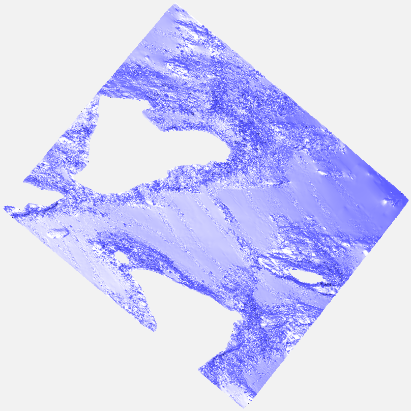
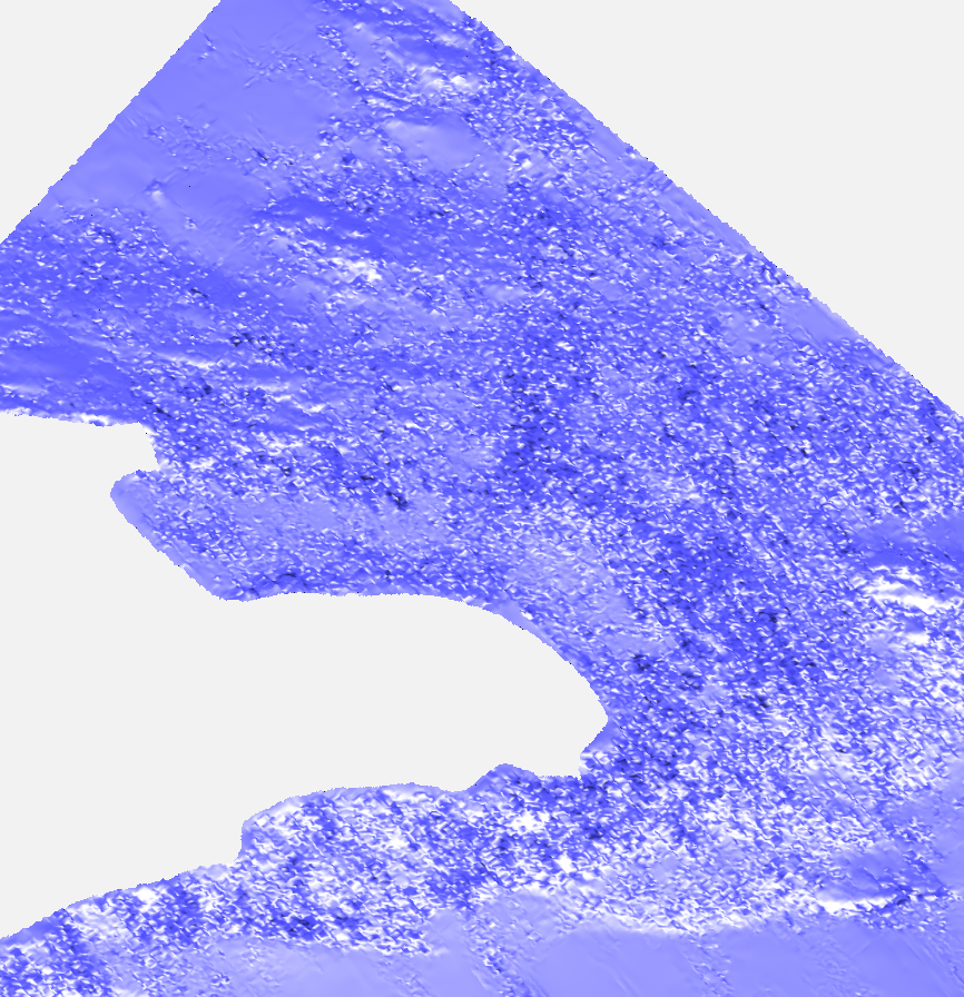
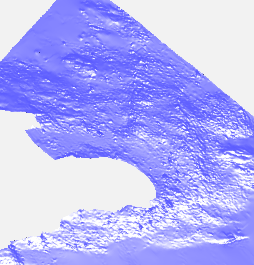
(a)	(b)	(c)

Figure 16: (a) Approximating surface according to setup V9 (variable strict threshold, 9 iterations). (b) Detail of surface in (a). (c) Corresponding detail for surface of setup V9E2 (as setup V9 with element size restriction)

8.2 Limit surfaces

The distances between a surface and the associated points vary depending on the extent of steepness or roughness in the sea bed/terrain and the point quality. In general, the distance will be larger in non-smooth areas. The point cloud can be bounded by limit surfaces, giving a means to enquire the uncertainty of the elevation represented by the given surface at every position in the surface domain. The limit surfaces share the spline space of the approximating surface and lies at opposite sides of the surface and the point cloud.

The initial point cloud is divided into two point clouds lying on either side of the approximating surface, from now on denoted the source surface. Each sub cloud give rise to a residual set, one corresponding to points lying above the source surface and one to points lying below. The residual sets are approximated individually by applying several iterations of the MBA-algorithm. The resulting surfaces are defined with the same collection of scaled tensor product B-splines as the source surface and no further refinement of the surfaces is performed. The resulting residual surfaces approximate the residual sets with high accuracy, but there might still be some residuals that exceed the corresponding residual surface.

A post process ensures interpolation of the remaining residuals. Given a residual $r_{a}$ at position $(x_{a},y_{a})$ where the distance $\Delta a=r_{a}-F_{upper}(x_{a},y_{a})>0$. Here $f_{upper}$ is the residual surface corresponding to the points lying above the source surface. Since the scaled tensor product B-splines $N_{B}$ of $F_{upper}$ have the partition of unity property, we know that

$$F_{upper}(x_{a},y_{a})+\Delta a=\sum_{B\in\mathcal{B}_{j}}(c_{B}+\Delta a)N_{B}(x_{a},y_{a})$$

following the notation of Equation 8. $\mathcal{B}_{j}$ is the collection of B-splines corresponding to of the residual surface. For each $B\in\mathcal{B}_{j}$ we add the maximum distance between the residuals in the B-spline support and the surface to the corresponding coefficients. This ensures that $F_{upper}(x_{a},y_{a})\geq r_{a}$ for all residuals. The lower limit surface is treated similarly. Finally, the two limit surfaces are created by adding the residual surfaces to the source surface.

An example of limit surfaces is shown in Fig. 17. The source surface is generated by Setup F7 in Tables 2 and 3. The maximum distance between the two limit surfaces is 4.26 meters, the minimum distance is zero, and the average distance is 0.93 meters. Seen from below, Fig. 17(a), the lower limit surface is dominant, but the upper limit surface can be glimpsed where the surfaces are tight. Similarly is the upper limit surface dominant when seen from above (b).

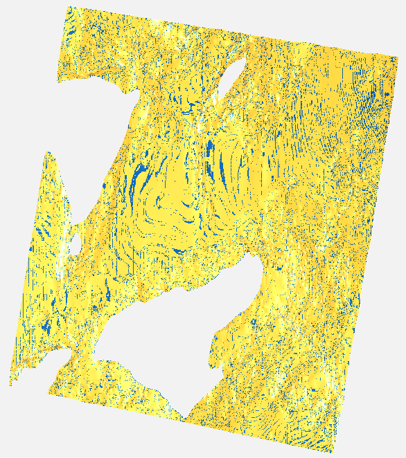
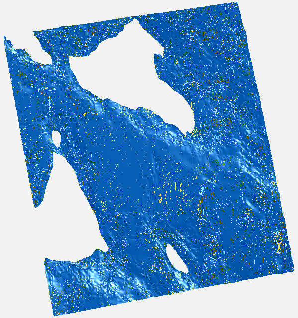
(a)	(b)

Figure 17: (a) Limit surfaces seen from below. (b) Limit surfaces seen from above.

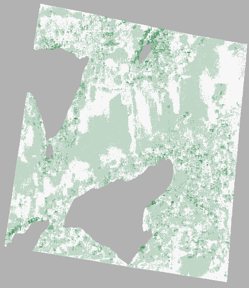
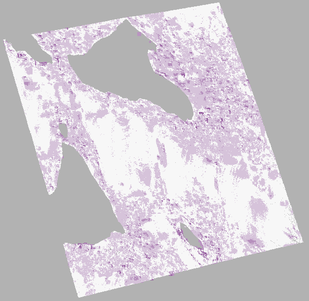
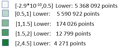
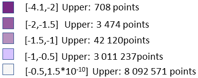
(a)	(b)

Figure 18: (a) Point cloud coloured according to the distance to the lower limit surface. (b) Point cloud coloured according to the distance to the upper limit surface.

In Fig. 18 the distances between the original point cloud and the limit surfaces are visualized (a) and (b). The points are coloured according to the distances to the associated surface and the colour scale and how the points are distributed with regard to distance are shown together with the surfaces. The distance range between the point cloud and the upper limit surface is $[-4.06m.,1.5\times 10^{-10}m.]$ and the average distance is 0.41 meters. The corresponding numbers for the lower limit surface are $[-2.0\times 10^{-10}m.,4.48m.]$ and 0.53 meters.

The upper limit surface is guaranteed to lie above all measurement points. Thus, it can serve as a conservative model with respect to the sea depth at shallows. A weighted surface between the source surface and the upper limit surface can be created to ensure a safety zone at shallows while restoring to the source surface at greater depths. Let $F_{w}$ be the weighted surface, $F_{source}$ the source surface and $F_{upper}$ the upper limit surface. The surfaces correspond to the same collection of B-splines. Following Equation 8 we have

$$F_{w}(u,v)= \alpha(u,v)F_{source}(u,v)+(1-\alpha(u_{B},v_{B}))F_{upper}(u,v)=$$

$$\sum_{B\in\mathcal{B}_{j}}\big{(}\alpha(u_{B},v_{B})c_{source,B}+(1-\alpha(u_{B},v_{B}))c_{upper,B}\big{)}N_{B}(u,v)$$

where the blending factor $\alpha$ depends on the elevation in a given point $(u,v)$ and a given elevation range $[d_{1},d_{2}]$ where the two surfaces are blended. The scaled B-spline $N_{B}$ is a scaled tensor product B-splines and the parameter value, $(u_{B},v_{B})$, of the coefficient corresponding to the B-spline is given by the knot vectors $\mathbf{u}=(u_{0},\ldots,u_{p_{1}+1})$ and $\mathbf{v}=(v_{0},\ldots,v_{p_{2}+1})$ of the B-spline as the Greville point

$$(u_{B},v_{B})=\Big{(}\sum_{j=1}^{p_{1}}\frac{u_{j}}{p_{1}},\sum_{k=1}^{p_{2}}\frac{v_{k}}{p_{2}}\Big{)}.$$

Let $d=0.5*(F_{source}(u_{B},v_{B})+F_{upper}(u_{B},v_{B}))$. Now, we can define $\alpha$ as

$$\alpha(u_{B},v_{B})=\begin{cases}1;&\text{if }d\leq d_{1},\\ 0;&\text{if }d\geq d_{2},\\ (d_{2}-d)/(d_{2}-d_{1});&\text{otherwise}.\end{cases}$$

Given $d_{2}=0$ and $d_{1}$ at a specified depth the weighted mid-surface will be close to the upper limit surface in shallow areas and coincide with the original approximating surface in deeper water.

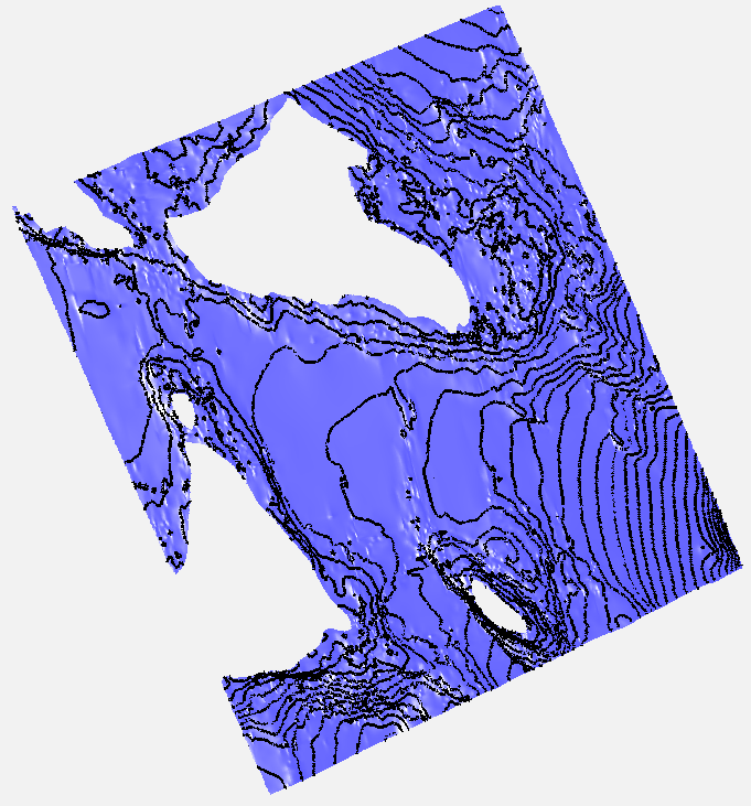
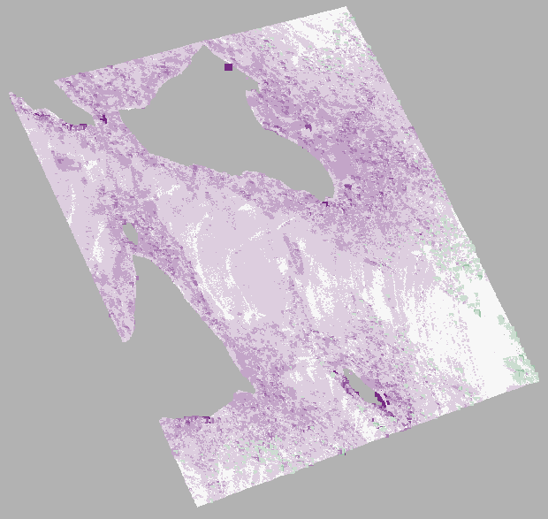
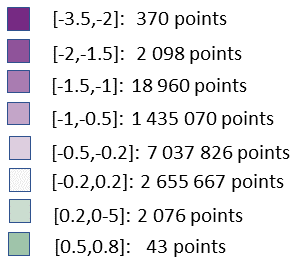
(a)	(b)

Figure 19: (a) Weighted mid surface with contour curves. (b) Data points coloured according to distance to weighted mid surface. The colour scale and number of points in each colour range is given.

A weighted middle surface for the approximating surface of Setup F7 and the corresponding upper limit surface is shown in Fig. 19(a) along with contour curves with resolution 1 meter. Here the limits of the transition zone are $d_{1}=-20$ and $d_{2}=0$. The contour curves differ slightly from the curves in Fig. 11, but the main pattern is the same. As seen in (b), the majority of the points lie below the surface. 2 119 points lie above the surface with a distance larger than 0.2 meters and these points are situated at the largest depths  in the data set. The maximum distances between the surface and the points are 0.76 meters above the surface and 3.22 meters below. The average distance is 0.32 meters.

8.3 Approximation with significant points

The weighted mid-surface construction can be vulnerable for outliers as the limit surface interpolates them. An approach for enforcing sufficient accuracy at shallows while maintaining a good overall accuracy is the concept of significant points.

Both least squares approximation and the MBA algorithm are able to weigh points individually. The surface will approximate points with a higher weight more closely and it is possible to do additional refinement in areas with significant points. In this construction the weight associated with significant points is five times the weight of ordinary points. Furthermore, an extra final iteration with the MBA method where significant points are weighted 50 times the weight of other points is applied if the accuracy at significant points does not satisfy the threshold. Thus, defining significant points at critical areas in shallow water and setting a stricter threshold for these points can address the need for a very accurate depth representation at shallows by a lean and smooth surface.

The election of significant points is crucial to get the wanted result: good accuracy in critical points, high safety at shallows, low data size and avoiding modelling of noise. We have selected 266 points from the original data set. The points lie in the vicinity of the extremal points shown in Fig. 15 (b). One data point close to each maximum point having a depth of less than ten meters, is selected as a significant point. The resulting points have the minimum depths of all data points in their neighbourhood. Fig. 20 (a) shows the resulting surface along with the significant points. In (b) also the surface from Setup F7 is included. The two surfaces are roughly similar, but differ slightly in some places. It is a tendency that the surface including approximation of significant points lie above the other in areas where the sea bed is smooth.

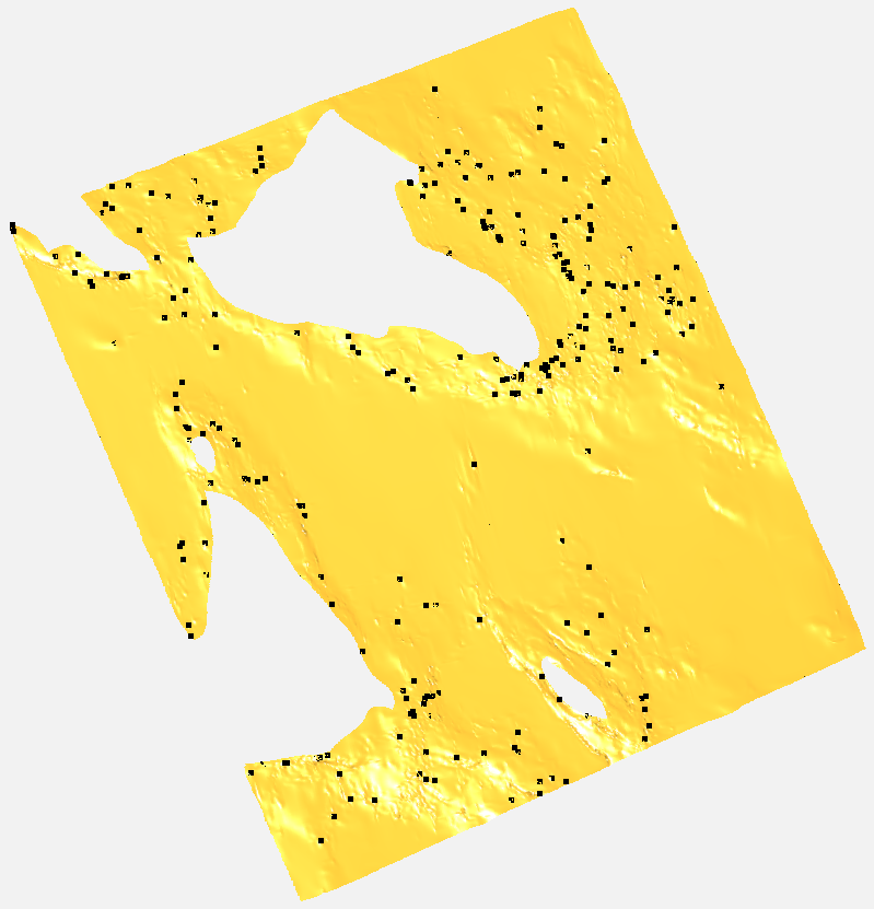
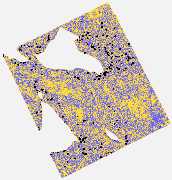
(a)	(b)

Figure 20: (a) Significant points with surface approximation. The threshold corresponding to the complete data set is 0.5 meters, while the threshold for the significant points is 0.2 meters (Setup FS7). (b) Surfaces from setup F7 and FS7. The significant points are included.

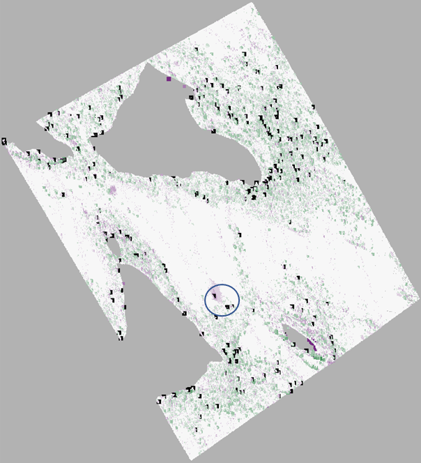
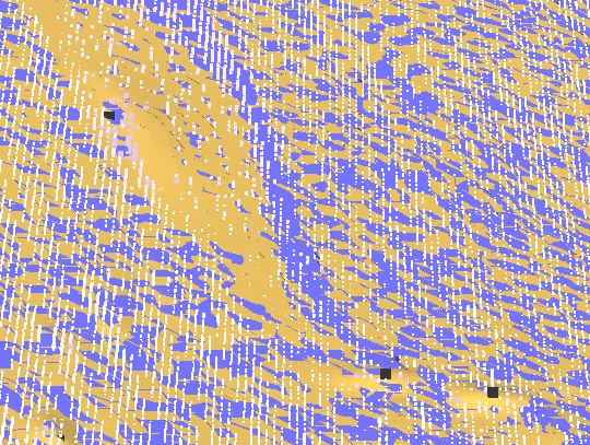
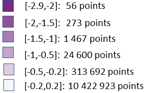
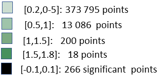
(a)	(b)

Figure 21: (a) Initial point cloud coloured according to the distance to the approximating surface where significant points have a stricter threshold. (b) Detail with both surfaces, the significant points and the initial point cloud in the area marked with s circle in (a).

Fig. 21 (a) shows the original point cloud coloured with respect to the distance to the surface fitting also significant points (Setup FS7) and the significant points. An area is marked for further study. The corresponding part of the two surfaces, the point cloud coloured according to distance and the significant points are shown in (b). The significant points tend to reduce the depth represented by the corresponding surface in an area in the vicinity of such a point.

Table 4: Figures of accuracy for approximations with different setups regarding the number of iterations, tolerance threshold, significant points and weighted mid surface construction. The three first cases are included from Table 3 as references.

Setup	Sf. size	No. coefs.	Max dist.	Av. dist.	$<$ 0.2	$<$ 0.5	$\geq$ 0.5
F7	2.5MB	33 830	2.85 m.	0.068 m.	10 429 550	685 381	35 179
V7	16MB	206 295	2.81 m.	0.052 m.	10 753 948	336 828	27 334
V9	139MB	1 830 313	2.48 m.	0.042 m.	10 957 497	179 908	12 705
WM7	2.5MB	33 830	3.49 m.	0.32 m.	2 655 667	7 037 902	1 456 541
FS7	2.6MB	35 491	2.9 m.	0.068 m.	10 422 923	687 487	39 700
FS9	17MB	217 934	2.47 m.	0.057 m.	10 669 437	459 456	21 217

Table 4 relates the weighted middle surface construction and approximation with significant points to pure point approximation. The weighted mid surface has lower accuracy than the other approaches. This is expected. The surface is lifted upwards to obtain a safety depth at shallows. The accuracy when significant points are included compares quite equitable to approximations without significant points, but the ordinary points are slightly punished for the extra emphasize on the significant points. For Setup FS7 and FS9 significant points with an associated tolerance of 0.2 are given. The maximum and average distance to the significant points after 7 iterations were 0.099 meters and 0.0008 meters, respectively, and the maximum distance between the surface and the points lying above the surface is 1.8 meters. After 9 iterations the maximum distance between the surface and the significant points is 0.023 meters and the average distance is 0.002 meters. The maximum distance to points above the surface is reduced to 1.68 meters. After 7 iterations, a final surface approximation with increased weight on the significant points was applied. This was not required using 9 iterations iteration steps.

9 Conclusion and further work

The LR B-spline surface format is a new representation format that provides a middle road between the rigid, but effective regularity of the raster format and the large flexibility of triangulated surfaces. LR B-spline surfaces are smooth and can, due to adaptivity, represent local detail without a drastic increase in data size. Being a novel format, it is not supported in GIS systems, but the surfaces can be exported as rasters in various resolutions as well as collections of tensor product spline surfaces.

Having a spline format, LR B-spline surfaces are well suited for computation of various properties. We have discussed the computation of contour curves and extremal points. The latter will require some post processing to get a clean collection of points. This will be looked into in the future. We will also look at a representation of slope and aspect that gives further insight in the information these quantities possess. We are for instance interested in a kind of contour curves for slope.

Generalization is the process of computing a lower resolution terrain or seabed model from a high resolution one. Advanced methods take features such as extremal points, ridges and valleys into account. Generalization is not yet investigated for LR B-spline representations, but it is an important and interesting topic for further work.

Outliers may obstruct the surface computation. Single points do not influence the surface significantly, but collection of outliers points and outliers in areas with sparse data points will drag the surface in their direction. Moreover, the existence of outliers will obstruct the accuracy information. To some extent outliers can be identified during the computation of the approximating surface and removed during the iterative algorithm presented in Section 3. However, this approach is mostly suited for single outlier points and there is always a risk of removing significant points. The outlier problem is an important topic for further work.

Ongoing research focuses on the approximation threshold and a stop criterion for the number of iterations in the approximation algorithm. The intent is to find a balance between the accuracy of the approximation and the number of coefficients representing the surface. The idea is to get an accurate surface that do not adapt to noise in the data.

Data availability The data set used in the computations belong to an area in Norway called Søre Sunnmøre where data is made generally available. The actual data set is from an older acquisition and are available on request.

References

- (1) Basso K., Zingano P., Freitas C. D. S., Interpolation of Scattered Data: Investigating Alternatives for the Modified Shepards Method. Conference: XII Brazilian Symposium on Computer Graphics and Image Processing (SIBGRAPI ’99), October 17-20, 1999, Campinas, Brazil
- (2) Bobach T., Umlauf G., Natural Neighbor Concepts in Scattered Data Interpolation and Discrete Function Approximation, In GILNI, Visulazation of Large and Unstructured Data Sets, 2007, 23–-35
- (3) Boehm, W., Inserting new knots into B-spline curves. Computer-Aided Design 12 (4), 1980, 199–201
- (4) Buhmann M. D., Radial basis functions. Acta Numerica. Cambridge University Press., 2000, 1–38
- (5) Dokken T., Pettersen K. F., Lyche T., Polynomial splines over locally refined box-partitions, Computer Aided Geometric Design, 30, 2013, 331–356
- (6) Dokken T., Skytt V., Intersection Algorithms and CAGD, In: Hasle G., Lie K.-A., Quak E. (eds) Geometric modelling, numerical simulation, and optimization: Applied mathematics at SINTEF, Springer Verlag, Berlin, Heidelberg, 2007, 41–90
- (7) Dokken, T. Skytt V., Barrowclough O., Trivariate Spline Representations for Computer Aided Design and Additive Manufacturing, Computers & Mathematics with Application, 78 (7), 2019, 2168–2182
- (8) Dokken T., Skytt V., SISL – SINTEF Spline Library, Reference Manual, Version 4.7, 2021, https://github.com/SINTEF-Geometry/SISL/
- (9) Fisher P. F., Tate N. J., Causes and consequences of error in digital elevation models. Progress in Physical Geography 30, 2006, DOI: 10.1191/0309133306pp492ra
- (10) Floater M. S., Hormann K., Surface Parameterization: a Totorial and Survey. Advances in Multiresolution for Geometric Modelling, Mathematics and Visualization, Dodgson N. A., Floater M. S., and Sabin M. A., editors, Springer, Berlin, Heidleber, 2005, 157–186
- (11) Forsey D. R., Bartels R. H., Hierarchical B-spline refinement. In: SIGGRAPH 88 conference proceedings, 4, 1988, 205–212
- (12) Franke R., Scattered Data Interpolation: Tests of Some Methods, Mathematics of Computation, 38(157): January 1982
- (13) Franke R., Nielson G., Smooth Interpolations of Large Sets of Scattered Data. International Journal for Numerical Methods in Engineering 15, 1980, 1691–1704.
- (14) Nelson E. J., Jones N. L., Miller A. W., Algorithm for precise drainage-basin delineation. Journal of Hydraulic Engineering, 120(3), 1994, 298–312
- (15) Lee S., Wolberg G., Shin S. Y., Scattered data interpolation with multilevel B-splines, IEEE Transaction on Visualization and Computer Graphics, 3(3), 1997, 229–244
- (16) Li Z. , Zhu Q. , Gold C., Digital Terrain Modeling Principles and Methodology. CRC Press (Taylor & Francis Group), 2005, ISBN: 9780415324625
- (17) Mehlum E., Skytt V., Surface Editing, In: Dælen M., Tveito A. (eds) Numerical Methods and Software Tools in Industrial Mathematics, Birkhäusser, Boston, 1997, 381–396
- (18) Mitas L., Mitasova H., In:Longley P., Goodchild M. F., Maguire D. J., Rhind D. W. (eds) Spatial interpolation, Geographic Information Systems - Principles, Techniques, Management, and Applications, 2005, 481–498
- (19) Nowacki H., Westgaard G., Heinemann J., Creation of Fair Surfaces Based on Higher Order Fairness Measures with Interpolation Constraints, In: Nowacki H., Kaklis P. D. (eds) Creating Fair and Shape-Preserving Curves and Surfaces, B. G. Teubner Stuttgart, Leipzig, 1998, 141–161
- (20) Oliver M. A. , Webster R. . Kriging: a method of interpolation for geographical information system, INT. J. Geographical Information Systems, 4(3), 1990, 323–332
- (21) Patrikalakis N.M, Maekawa T., Shape Interrogation for Computer Aided Design and Manufacturing, Springer, Heidelberg, 2002
- (22) Patrizi F., Dokken T., Linear dependence of bivariate Minimal Support and Locally Refined B-splines over LR-meshes, Computer Aided Geometric Design, 77, 2020
- (23) Sederberg T. W., Zheng J., Bakenov A., Nasri A., T-splines and T-NURCCs, ACM Trans. Graph., 22 (3), 2003, 477–484
- (24) Shepard D., A Two-Dimensional Interpolation Function for Irregularly Spaced Data, Proc. 23rd Nat. Conf. ACM, 1968, 517–523
- (25) Scott, M. A., LI, X., Sederberg T. W., Hughes T. J. R., Local refinement of analysis-suitable T-splines, Computer Methods in Applied Mechanics and Engineering, Volumes 213–216, 2012, 206–222
- (26) Skytt V., Barrowclough O., Dokken T., Locally refined spline surfaces for representation of terrain data, Computers & Graphics, 49, 2015, 58–68
- (27) Skytt V., Dokken T., Dahl H. E. I., Harpham Q., Deconfliction, surface generation and LR B-splines, In: Floater M., Lyche T., Mazure M.-L., Mørken K. (eds) Mathematical Methods for Curves and Surfaces: 9th International Conference, MMCS 2016 Tønsberg, Norway, June 23-28 Revised Selected Papers, Springer Publishing Company, 2016, 270–295
- (28) Skytt V., Dokken T., Scattered data approximation by LR B-spline surfaces. A study on refinement strategies for efficient approximation. ArXiv:2012.08130. To appear in the the Springer INdAM volume entitled ”Geometric Challenges in Isogeometric Analysis”, 2021
- (29) Skytt V., A Recursive Approach to Surface-surface Intersections In: Dæhlen M., Mørken K., Schumaker L. L. (eds) Mathematical Methods for Curves and Surfaces: Tromsø 2004 conference proceeding, Nashboro Press, Brentwood 2004, 327–338
- (30) Vivoni E. R., Ivanov V. Y., Bras R. L., Entakhabi D., Triangulated Irregular Networks Based on Hydrological Similarity. Journal of Hydrologic Engineering 9(4) https://doi.org/10.1061/(ASCE)1084-0699(2004)9:4(288), 2004
- (31) Wise S., Geomorphotmetry and DEM Error. Geomorphometry.org/2011
- (32) Wise S., Cross-validation as a means of investigating DEM interpolation error. Computers & Geosciences 37, 2011, 978–991
- (33) Zhang W., Tang Z., Li J, Adaptive Hierarchical B-spline Surface Approximation of Large-scale Scattered Data, In: Proc. Pacific Graphics 98. Sixt Pacific Conference. 8–16, 1998