BayesAdapter: Being Bayesian, Inexpensively and Reliably, via Bayesian Fine-tuning

Abstract

Despite their theoretical appealingness, Bayesian neural networks (BNNs) are left behind in real-world adoption, mainly due to persistent concerns on their scalability, accessibility, and reliability. In this work, we develop the BayesAdapter framework to relieve these concerns. In particular, we propose to adapt pre-trained deterministic NNs to be variational BNNs via cost-effective Bayesian fine-tuning. Technically, we develop a modularized implementation for the learning of variational BNNs, and refurbish the generally applicable exemplar reparameterization trick through exemplar parallelization to efficiently reduce the gradient variance in stochastic variational inference. Based on the lightweight Bayesian learning paradigm, we conduct extensive experiments on a variety of benchmarks, and show that our method can consistently induce posteriors with higher quality than competitive baselines, yet significantly reducing training overheads. Code is available at https://github.com/thudzj/ScalableBDL.

1 Introduction

Much effort has been devoted to developing expressive Bayesian neural networks (BNNs) to make accurate and reliable decisions (MacKay, 1992; Neal, 1995; Graves, 2011; Blundell et al., 2015). The principled uncertainty quantification capacity of BNNs is critical for realistic decision-making, finding applications in scenarios ranging from model-based reinforcement learning (Depeweg et al., 2016), active learning (Hernández-Lobato and Adams, 2015) to healthcare (Leibig et al., 2017) and autonomous driving (Kendall and Gal, 2017). BNNs are also known to be capable of resisting over-fitting and over-confidence.

Nonetheless, BNNs are falling far behind in terms of adoption in real-world applications compared with deterministic NNs (He et al., 2016a; Vaswani et al., 2017), due to various issues. For example, typical approximate inference methods for BNNs are often difficult to simultaneously maintain efficacy and scalability (Zhang et al., 2018; Maddox et al., 2019). Implementing a BNN algorithm requires substantially more expertise than implementing a deterministic NN program. Moreover, as revealed, BNNs trained from scratch without the “cold posterior” trick are often systematically worse than their point-estimate counterparts in terms of predictive performance (Wenzel et al., 2020a); some easy-to-use BNNs (e.g., Monte Carlo dropout) tend to suffer from mode collapse in function space, thus usually give uncertainty estimates of poor fidelity (Fort et al., 2019).

To mitigate these issues, we develop a pre-training & fine-tuning workflow for learning variational BNNs given an inherent connection between variational BNNs (Blundell et al., 2015) and regular deep neural networks (DNNs). The resultant BayesAdapter framework learns a variational BNN by performing several rounds of Bayesian fine-tuning, starting from a pre-trained deterministic NN. BayesAdapter is effective and lightweight, and conjoins the complementary benefits from deterministic training and Bayesian reasoning, e.g., performance matching the pre-trained deterministic models, resistance to over-fitting, reliable uncertainty estimates, etc. (find evidence in Figure 1).

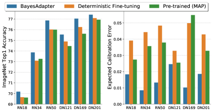
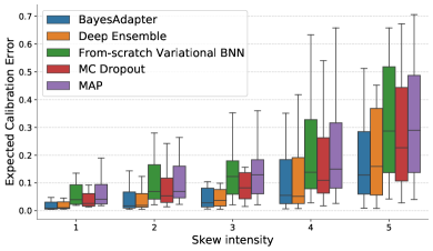
Figure 1: (Left): BayesAdapter boosts the accuracy of ImageNet classifiers without compromising model calibration (estimated by expected calibration error (ECE) (Guo et al., 2017)). By contrast, deterministic fine-tuning only marginally improves the accuracy of pre-trained models yet aggravates over-confidence. RN refers to ResNet (He et al., 2016a) and DN refers to DenseNet (Huang et al., 2017). (Right): BayesAdapter learns a CIFAR-10 classifier which approaches or outperforms competing baselines in terms of ECE for CIFAR-10 corruptions (Hendrycks and Dietterich, 2019). Each box summarizes the ECE across 19 types of skew. We perform Bayesian fine-tuning for only 4 and 12 epochs on ImageNet and CIFAR-10 respectively. More details are deferred to Sec 4.

To improve the usability of BayesAdapter, we provide a modularized implementation for the stochastic variational inference (SVI) under multiple representative variational distributions, including mean-field Gaussian and parameter-sharing ensemble. Reducing the variance of stochastic gradients is crucial for stabilizing and accelerating SVI, while the pioneering works such as local reparameterization (Kingma et al., 2015) and Flipout (Wen et al., 2018) can only deal with specific variational distributions, e.g., Gaussians and distributions whose samples can be reparameterized with symmetric perturbations. To tackle this issue, we refurbish the widely-criticized exemplar reparameterization (Kingma et al., 2015) by accelerating the exemplar-wise computations through parallelization, giving rise to an efficient and general-purpose gradient variance reduction technique.

We conduct extensive experiments to validate the advantages of BayesAdapter over competing baselines, in aspects covering efficiency, predictive performance, and quality of uncertainty estimates. Desirably, we scale up BayesAdapter to big data (e.g., ImageNet (Deng et al., 2009)), deep architectures (e.g., ResNets (He et al., 2016a)), and practical scenarios (e.g., face recognition (Deng et al., 2019)), and observe promising results. We also perform a series of ablation studies to reveal the characteristics of the proposed approach.

2 Background

In this section, we motivate BayesAdapter by drawing a connection between variational BNNs and DNNs trained by maximum a posteriori (MAP) estimation.

Let $\mathcal{D}=\{({\bm{x}}^{(i)},y^{(i)})\}_{i=1}^{n}$ be a given training set, where ${\bm{x}}^{(i)}\in\mathbb{R}^{d}$ and $y^{(i)}\in\mathcal{Y}$ denote the input data and label, respectively. A DNN model can be fit via MAP estimation:

$$\small{\max_{\bm{w}}\frac{1}{n}\sum_{i}[\log p(y^{(i)}|{\bm{x}}^{(i)};\bm{w})]+\frac{1}{n}\log p(\bm{w})}.$$ (1)

We use $\bm{w}\in\mathbb{R}^{p}$ to denote the high-dimensional model parameters, with $p(y|\bm{x};\bm{w})$ as the predictive distribution associated with the model. The prior $p(\bm{w})$, when taking the form of an isotropic Gaussian $\mathcal{N}(\bm{w};\bm{0},\sigma^{2}_{0}\mathbf{I})$, reduces to the weight decay regularizer with coefficient $\lambda=1/(\sigma_{0}^{2}n)$ in optimization. Nevertheless, deterministic training may easily cause over-fitting and over-confidence, rendering the learned models of poor reliability (see Figure 1). Naturally, BNNs come into the picture to address these limitations.

Typically, BNNs learn by inferring the posterior $p(\bm{w}|\mathcal{D})$ given the prior $p(\bm{w})$ and the likelihood $p(\mathcal{D}|\bm{w})$. Among the wide spectrum of BNN algorithms (MacKay, 1992; Neal, 1995; Graves, 2011; Blundell et al., 2015; Liu and Wang, 2016; Gal and Ghahramani, 2016), variational BNNs are particularly promising due to their analogy to ordinary backprop. Formally, variational BNNs use a $\bm{\theta}$-parameterized variational distribution $q(\bm{w}|\bm{\theta})$ to approximate $p(\bm{w}|\mathcal{D})$, by maximizing the evidence lower bound (ELBO) (scaled by $1/n$):

$$\small{\max_{\bm{\theta}}\underbrace{\mathbb{E}_{q(\bm{w}|\bm{\theta})}\big{[}\frac{1}{n}\sum_{i}\log p(y^{(i)}|{\bm{x}}^{(i)};\bm{w})\big{]}}_{\mathcal{L}_{ell}}\underbrace{\vphantom{\big{[}\frac{1}{n}\sum_{i}\log p(y^{(i)}|{\bm{x}}^{(i)};\bm{w})\big{]}}-\frac{1}{n}D_{\mathrm{KL}}\left(q(\bm{w}|\bm{\theta})\|p(\bm{w})\right)}_{\mathcal{L}_{c}}},$$ (2)

where $\mathcal{L}_{ell}$ is the expected log-likelihood and $\mathcal{L}_{c}$ is the complexity loss. By casting posterior inference into optimization, Eq. (2) makes the training of BNNs resemble that of DNNs. After training, the variational posterior is leveraged for prediction through marginalization:

$$\small p(y|\bm{x},\mathcal{D})\approx\mathbb{E}_{q(\bm{w}|\bm{\theta})}p(y|\bm{x};\bm{w})\approx\frac{1}{S}\sum_{s=1}^{S}p(y|\bm{x};\bm{w}^{(s)}),$$ (3)

where $\bm{w}^{(s)}\sim q(\bm{w}|\bm{\theta}),s=1,...,S$, with $S$ denoting the number of Monte Carlo (MC) samples. Eq. (3) is known as posterior predictive, Bayes ensemble, or Bayes model average.

We can simultaneously quantify the epistemic uncertainty with these MC samples. A principled uncertainty metric is the mutual information between the model parameter and the prediction (Smith and Gal, 2018), estimated by ($H$ denotes the Shannon entropy):

$$\small\mathcal{I}({\bm{w}},y|{\bm{x}},\mathcal{D})\approx H\left(\frac{1}{S}\sum_{s=1}^{S}p(y|\bm{x};\bm{w}^{(s)})\right)-\frac{1}{S}\sum_{s=1}^{S}H\left(p(y|\bm{x};\bm{w}^{(s)})\right).$$ (4)

However, most of the existing variational BNNs exhibit limitations in scalability and performance (Osawa et al., 2019; Wenzel et al., 2020a), compared with their deterministic counterparts. This is mainly due to the higher difficulty of learning high-dimensional distributions from scratch than point estimates.

Given that MAP converges to a mode of the Bayesian posterior, it might be plausible to adapt pre-trained deterministic DNNs to be Bayesian economically. Following this hypothesis, we repurpose the converged parameters $\bm{w}^{*}$ of MAP – take $\bm{w}^{*}$ as the initialization of the parameters of the approximate posterior. Laplace approximation (MacKay, 1992) is a classic method in this spirit, which assumes a Gaussian approximate posterior, and adapts ${\bm{w}}^{*}$ and the local curvature at ${\bm{w}}^{*}$ as the Gaussian mean and variance respectively. Yet, Laplace approximation is inflexible and usually computationally prohibitive (only after the introduction of Gauss-Newton approximation, KFAC approximation, and particularly the last-layer approximation, the cost of Laplace approximation becomes affordable (Daxberger et al., 2021)). Alternatively, we develop the more practical Bayesian fine-tuning scheme, whose core notion is to fine-tune the imperfect approximate posterior by maximizing ELBO.

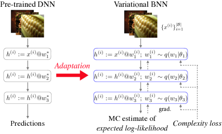
Figure 2: BayesAdapter adapts pre-trained DNNs to be variational BNNs and then launches few rounds of Bayesian fine-tuning. We provide a modularized implementation for Bayesian fine-tuning, allowing users to learn a variational BNN as if training a DNN under a weight decay regularizer.

3 BayesAdapter

We describe BayesAdapter in this section. Figure 2 gives its illustration.

In BayesAdapter, the configuration of the variational distribution $q({\bm{w}}|{\bm{\theta}})$ plays a decisive role. Although a wealth of variationals have emerged for adoption (Louizos and Welling, 2016; Li and Turner, 2017; Wen et al., 2018), on one hand, more complicated ones (Louizos and Welling, 2017; Shi et al., 2018b) are routinely accompanied by less scalable learning; on the other hand, the aforementioned hypothesis inspiring Bayesian fine-tuning entails an explicit alignment between the DNN parameters ${\bm{w}}^{*}$ and the variational parameters ${\bm{\theta}}$. Thus, we primarily concern the typical mean-field Gaussian distribution as well as a more powerful one that resembles Deep Ensemble (Lakshminarayanan et al., 2017).

3.1 Mean-field Gaussian (MFG) Variational

Without losing generality, we write the MFG variational as $q({\bm{w}}|{\bm{\theta}})=\mathcal{N}({\bm{w}};{\bm{\mu}},\textbf{diag}(\exp(2\bm{\psi})))$, with ${\bm{\mu}},\bm{\psi}\in\mathbb{R}^{p}$ denoting the mean and the logarithm of standard deviation respectively. In this sense, we can naturally initialize ${\bm{\mu}}$ with ${\bm{w}}^{*}$ at the beginning of fine-tuning to ease approximate inference and to enable the investigation of more qualified posterior modes. As in MAP, we also assume an isotropic Gaussian prior $p(\bm{w})=\mathcal{N}(\bm{w};\bm{0},\sigma^{2}_{0}\mathbf{I})$. Then the gradients of the complexity loss can be derived analytically:

$$\small\nabla_{{\bm{\mu}}}\mathcal{L}_{c}=-\lambda{{\bm{\mu}}},\;\;\nabla_{\bm{\psi}}\mathcal{L}_{c}=-\lambda{\exp(2\bm{\psi})}+\frac{1}{n},\;\;\text{with}\;\lambda=\frac{1}{\sigma_{0}^{2}n}.\vspace{-0.0cm}$$ (5)

Intuitively, the above gradients for the variational parameters correspond to a variant of the vanilla weight decay in DNNs. Having identified this, we can implement a module similar to weight decay to implicitly be responsible for the complexity loss, leaving only the expected log-likelihood $\mathcal{L}_{ell}$ required to be explicitly handled. We will elaborate on the details of solving $\max\mathcal{L}_{ell}$ after presenting a more expressive variational configuration.

3.2 Parameter-sharing Ensemble (PSE) Variational

Despite simplicity, the MFG variational can be limited in expressiveness for capturing the multi-modal parameter posterior of over-parameterized neural networks. Empowered by the observation that Deep Ensemble (Lakshminarayanan et al., 2017) is a compelling Bayesian marginalization mechanism in deep learning (Wilson and Izmailov, 2020), we intend to develop a low-cost ensemble-like variational for more practical Bayesian deep learning.

Specifically, we first define the variational as a uniform mixture of $C$ Gaussians: $q({\bm{w}}|{\bm{\theta}})=\frac{1}{C}\sum_{c}\mathcal{N}({\bm{w}};{\bm{w}}^{(c)},\bm{\Sigma}^{(c)})$, where $\bm{\Sigma}^{(c)}\in\mathbb{R}^{p\times p}$ is positive-definite and its elements are independent of the dimension $p$. In this sense, the complexity loss boils down to the KL divergence between a mixture of Gaussians and a Gaussian, which, yet, cannot be calculated analytically in general. Nevertheless, under the mild assumption that ${\bm{w}}^{(c)}\in\mathbb{R}^{p}$ is normally distributed and $p$ is large enough, the KL divergence can be approximated by a weighted sum of the KL divergences between the Gaussian components and the Gaussian prior (refer to (Gal and Ghahramani, 2015) for detailed discussion and proof). Namely,

$$-\frac{1}{n}D_{\mathrm{KL}}\left(\frac{1}{C}\sum_{c}\mathcal{N}({\bm{w}};{\bm{w}}^{(c)},\bm{\Sigma}^{(c)})\big{\|}\mathcal{N}(\bm{w};\bm{0},\sigma^{2}_{0}\mathbf{I})\right)$$ (6)

$$\approx -\frac{1}{2\sigma_{0}^{2}nC}\sum_{c=1}^{C}\left(\|{\bm{w}}^{(c)}\|_{2}^{2}+\text{trace}(\bm{\Sigma}^{(c)})-\sigma_{0}^{2}\log|\bm{\Sigma}^{(c)}|\right)+\text{constant}.$$

Based on the observation that Bayesian model average benefits significantly more from the exploration of new modes than navigation around a local mode (Wilson and Izmailov, 2020), we assume $\bm{\Sigma}^{(c)},c=1,...,C$, to be a constant diagonal matrix $\sigma^{2}\mathbf{I}$ with $\sigma^{2}$ approaching ${0}$. Namely, we purely chase multi-mode exploration and leave the joint optimization of $\bm{\Sigma}^{(c)}$ and ${\bm{w}}^{(c)}$ for future investigation. Then, $q({\bm{w}}|{\bm{\theta}})$ almost amounts to a mixture of deltas (i.e., an ensemble) and with high probability we can approximate the realisation of ${\bm{w}}$ by a uniform sample from $\{{\bm{w}}^{(1)},...,{\bm{w}}^{(C)}\}$. Meanwhile, the complexity loss approximately becomes $-\frac{\lambda}{2C}\sum_{c=1}^{C}\|{\bm{w}}^{(c)}\|_{2}^{2}+\text{constant}$, and we can easily implement a weight decay-like module to be responsible for its gradient. We comment here that it may be more plausible to alternatively leverage the rigorous quasi-KL divergence (Hron et al., 2018) for estimating the divergence between a mixture of deltas and the Gaussian prior, left as a future work.

Simulating an ensemble is far from our ultimate goal due to the required high cost. To make the variational economical, we explore a valuable insight from recent works (Wen et al., 2020; Wenzel et al., 2020b) that the parameters of different ensemble components can be partially shared without undermining effectiveness.

Specifically, abusing ${\bm{w}}$ to notate the parameter matrix of size $m_{\text{in}}\times m_{\text{out}}$ in a neural network layer, we generate $C$ components via: ${\bm{w}}^{(c)}={\bm{l}}^{(c)}{\bm{r}}^{(c)}\circ\bar{{\bm{w}}},c=1,...,C$, where $\bar{{\bm{w}}}\in\mathbb{R}^{m_{\text{in}}\times m_{\text{out}}}$ are the shared parameters and ${\bm{l}}^{(c)}\in\mathbb{R}^{m_{\text{in}}\times r}$ and ${\bm{r}}^{(c)}\in\mathbb{R}^{r\times m_{\text{out}}}$ correspond to $r$-rank decomposition of some perturbations. $\circ$ is element-wise multiplication. The shared parameters $\bar{{\bm{w}}}$ can be initialized as ${\bm{w}}^{*}$ to ease and speedup Bayesian fine-tuning. When the rank $r$ is suitably small, the above design can significantly reduce the model size, and save the training effort. Of note that the previous works (Wen et al., 2020; Wenzel et al., 2020b) confine $r$ to be 1 to permit the adoption of a specific gradient variance reduction trick. Conversely, we loosen this constraint by using a more generally applicable variance reduction tactic, detailed below.

3.3 A Reliable Estimation of the Expected Log-likelihood $\mathcal{L}_{ell}$

Given the high non-linearity of deep NNs and the large volume of data in real-world scenarios, we follow the stochastic variational inference (SVI) paradigm for estimating $\mathcal{L}_{ell}$. Formally, given a mini-batch of data $\mathcal{B}=\{({\bm{x}}^{(i)},y^{(i)})\}_{i=1}^{|\mathcal{B}|}$, we solve

$$\small\max_{\bm{\theta}}\mathcal{L}^{\prime}_{ell}=\frac{1}{|\mathcal{B}|}\sum_{i=1}^{|\mathcal{B}|}\log p(y^{(i)}|{\bm{x}}^{(i)};\bm{w}),$$ (7)

where ${\bm{w}}$ is drawn from the MFG or PSE variational via reparameterization (Kingma and Welling, 2013). The gradients w.r.t. the variational parameters can be derived automatically with autodiff libraries, thus the training resembles that of regular DNNs.

However, gradients derived by $\mathcal{L}^{\prime}_{ell}$ might exhibit high variance, caused by sharing the sampled parameters ${\bm{w}}$ across data in the mini-batch (Kingma et al., 2015). Popular techniques for addressing this issue typically assume a restrictive form of variational distribution (Kingma et al., 2015; Wen et al., 2018), struggling to handle structured distributions like the proposed PSE with $>1$ rank. Fortunately, there is a generally applicable strategy for reducing gradient variance in stochastic variational inference named exemplar reparametrization (ER), which samples dedicated parameters for every exemplar in the minibatch for estimating $\mathcal{L}_{ell}$:

$$\small\mathcal{L}_{ell}^{*}=\frac{1}{|\mathcal{B}|}\sum_{i=1}^{|\mathcal{B}|}\log p(y^{(i)}|{\bm{x}}^{(i)};\bm{w}^{(i)}),\;\bm{w}^{(i)}\stackrel{{\scriptstyle\text{i.i.d.}}}{{\sim}}q({\bm{w}}|{\bm{\theta}}),\;i=1,...,|\mathcal{B}|.$$ (8)

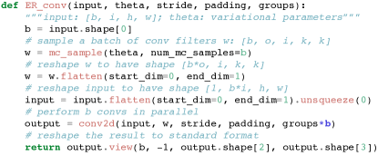
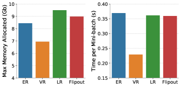
Figure 3: (Left): Implementation of exemplar reparametrization for 2D convolution in PyTorch (Paszke et al., 2019). (Right): Memory and time cost comparison among exemplar reparametrization (ER), vanilla reparametrization (VR) (Kingma and Welling, 2013), local reparametrization (LR) (Kingma et al., 2015), and Flipout (Wen et al., 2018) with mean-field Gaussian variational used (estimated on ImageNet with ResNet-50 architecture).

We can see that the computational cost of ER is identical to that of vanilla reparameterization, but ER was criticized for that the involved exemplar-wise computations could not be efficiently done within the popular computation libraries in 2015 (Kingma et al., 2015). With the rapid development of high-performance device-propriety kernel backends (e.g. cuDNN (Chetlur et al., 2014)) in recent years, we wonder is the criticism still hold? To this end, we first refurbish ER to fit nowadays ML frameworks. Our key insight here is to perform multiple exemplar-wise computations in parallel with a single kernel launch, e.g., organize exemplar-wise matrix multiplications as a batch matrix multiplication; organize exemplar-wise convolutions as a group convolution (see Figure 3 (Left)). We then conduct an empirical study on the computation cost of ER and relevant methods using MFG variational. Figure 3 (Right) shows the results.

Surprisingly, ER’s time efficiency is comparable with that of local reparameterization (Kingma et al., 2015) and Flipout (Wen et al., 2018), while its memory cost is even lower. This is perhaps because local reparameterization and Flipout both need to calculate and store one extra mini-batch of feature maps, which are rather large in ImageNet models. Note that the added memory cost of ER upon vanillar reparameterization comes from the storage of a mini-batch of temporary parameters. We clarify that the primary merit of ER over existing methods is the higher generality rather than better learning outcomes. We hope that ER will benefit the further development of new variational distributions.

3.4 A Plug-and-play Library

We wrap the details of the aforementioned modularized stochastic variational inference and ER strategy for MFG and PSE in a plug-and-play Python library to free the users from the difficulties of implementing BayesAdapter.

4 Experiments

We apply BayesAdapter to a diverse set of benchmarks for empirical verification.

Settings. In general, we pre-train DNNs following standard protocols or fetch the pre-trained checkpoints available online, and then perform Bayesian fine-tuning. We randomly initialize the newly added variational parameters (e.g., $\bm{\psi}$, ${\bm{l}}^{(c)},{\bm{r}}^{(c)}$). Unless otherwise stated, we set $r=1$ and $C=20$ for PSE and use the ER trick during training. We use $S=20$ MC samples to make prediction and quantify epistemic uncertainty. We conduct experiments on 8 RTX 2080Ti GPUs. Full details are deferred to Appendix B.

Table 1: Comparison on test accuracy and negative log-likelihood (NLL) on CIFAR-10 benchmark. We use underline to emphasize the results obtained given significantly more training effort. For BayesAdapter, we repeat every experiment for 3 times and report the error bar.

Method	Accuracy (%) $\uparrow$	NLL $\downarrow$
MAP	96.92	0.1312
Laplace Approx.	96.41	0.1204
MC Dropout	96.95	0.1151
SWAG	96.32	0.1122
Deep Ensemble	97.40	0.0869
VBNN (MFG)	96.95	0.0994
VBNN (PSE)	96.88	0.1328
BayesAdapter (MFG)	97.10$\pm$0.03	0.1007$\pm$0.0014
BayesAdapter (PSE)	97.13$\pm$0.03	0.0936$\pm$0.0010

Baselines. We consider extensive baselines including: (1) MAP, which is the fine-tuning start point, (2) Laplace Approx.: which preforms Laplace approximation with diagonal Fisher information matrix, (3) MC Dropout, which is a dropout variant of MAP, (4) VBNN, which refers to from-scratch trained variational BNNs. In particular, the variational BNN methods like BayesAdapter and VBNN are evaluated on both the MFG and PSE variationals. We also include Deep Ensemble (Lakshminarayanan et al., 2017), and SWAG (Maddox et al., 2019) as baselines on CIFAR-10 benchmark (Krizhevsky et al., 2009).

4.1 CIFAR-10 Classification

We first conduct experiments on CIFAR-10 with wide-ResNet-28-10 architecture (Zagoruyko and Komodakis, 2016). We perform Bayesian fine-tuning for 12 epochs with the weight decay coefficient $\lambda$ set as 2e-4. Table 1 outlines the comparison on prediction performance.

It is worth noting that BayesAdapter substantially outperforms MAP, Laplace Approx., and MC Dropout in aspect of predictive performance. BayesAdapter also surpasses SWAG due to that SWAG does not directly benefit from high-performing pre-trained MAP models. The accuracy upper bound is Deep Ensemble, which trains 5 isolated MAPs and assembles their predictions to explicitly investigate diverse function modes, but it is much more expensive than BayesAdapter. VBNN is clearly defeated by BayesAdapter, confirming our claim that performing Bayesian fine-tuning from the converged deterministic checkpoints is beneficial to explore more qualified posteriors. BayesAdapter (PSE) surpasses BayesAdapter (MFG), especially in the aspect of NLL. Unless specified otherwise, we refer to BayesAdapter (PSE) as BayesAdapter in the following.

Converged ELBO. We compare the converged (training) ELBO of BayesAdapter and VBNN: the former gives $\mathcal{L}_{ell}=-0.019$ and $\mathcal{L}_{c}=-2806.8$ while the latter gives $\mathcal{L}_{ell}=-0.032$ and $\mathcal{L}_{c}=-2384.3$. This implies that Bayesian fine-tuning makes the approximate posterior converge to somewhere with better data fitting than from-scratch VI.

CIFAR-10 corruptions. We then assess the quality of predictive uncertainty on CIFAR-10 corruptions (Hendrycks and Dietterich, 2019). Figure 1 (Right) shows the results, which reflect the efficacy of BayesAdapter for promoting model calibration.

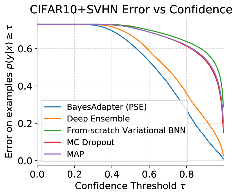
Figure 4: Error vs. confidence plots for models trained on CIFAR-10 and tested on both CIFAR-10 and SVHN.

CIFAR-10 vs SVHN. Following He et al. (2020), we evaluate the trained models on both CIFAR-10 and SVHN (Netzer et al., 2011) test sets. For every confidence threshold $0\leq\tau<1$, we compute the average error rate for predictions with $\geq\tau$ confidence (all predictions on SVHN data are regarded as incorrect). We depict the error vs. confidence curves in Figure 4. It is clear that BayesAdapter (PSE) has made more conservative predictions on the out-of-distribution (OOD) SVHN data than all baselines. BayesAdapter (PSE) even outperforms the expensive Deep Ensemble, implying that the parameter-sharing mechanism may impose further regularization on learning. The comparison also confirms from-scratch variational BNNs, even with the PSE variational, have difficulties to find good posteriors.

Speedup. BayesAdapter requires 200 epochs of deterministic training plus 12 epochs of variational training, while VBNN requires 200 epochs of variational training. Considering the cost of variational training is several times (about 2.1$\times$) that of deterministic training, the training time saved by BayesAdapter is considerable.

Table 2: Comparison on test accuracy and NLL on ImageNet benchmark.

Method	Accuracy (%) $\uparrow$	NLL $\downarrow$
MAP	76.13	0.9618
Laplace Approx.	75.89	0.9739
MC Dropout	74.88	0.9884
VBNN (MFG)	75.97	0.9435
VBNN (PSE)	75.12	0.9865
BayesAdapter (MFG)	76.45$\pm$0.05	0.9303$\pm$0.0005
BayesAdapter (PSE)	76.80$\pm$0.03	0.9159$\pm$0.0010

4.2 ImageNet Classification

We then scale up BayesAdapter to ImageNet with ResNet-50 (He et al., 2016a) architecture. We launch fine-tuning for merely 4 epochs with the weight decay coefficient $\lambda$ set as 1e-4.

Table 2 reports the empirical comparison. As expected, most results are consistent with those on CIFAR-10. On this large-scale scenario, it is more clear that the from-scratch learning baseline VBNN would suffer from local optima. The striking improvement of BayesAdapter upon MAP validates the benefits of Bayesian treatment. Zooming in, we also note that BayesAdapter (PSE) reveals remarkably higher accuracy than BayesAdapter (MFG), testifying the superior expressiveness of PSE over MFG.

Table 3: Accuracy $\uparrow$ comparison on open-set face recognition with MobileNetV2 architecture.

Method	LFW	CPLFW	CALFW	CFP-FF	CFP-FP
MAP	98.2%	84.0%	87.6%	97.8%	92.7%
MC Dropout	98.2%	83.6%	87.3%	97.8%	92.8%
BayesAdapter (MFG)	98.4%	83.9%	85.8%	97.6%	92.9%
BayesAdapter (PSE)	98.4%	84.7%	87.8%	97.8%	93.1%

Table 4: Ablation study on the rank $r$ of PSE. (ImageNet)

Method	Accuracy (%)	# of Param. (M)
MAP	76.13	25.56
BayesAdapter (PSE, $r$=1)	76.80	27.21
BayesAdapter (PSE, $r$=8)	76.78	38.76
BayesAdapter (PSE, $r$=16)	76.80	51.95

4.3 Face Recognition

To demonstrate the universality of BayesAdapter, we further apply it to the challenging face recognition task based on MobileNetV2 architecture (Sandler et al., 2018). We train models on the CASIA dataset (Yi et al., 2014), and perform comprehensive evaluation on face verification datasets including LFW (Huang et al., 2007), CPLFW (Zheng and Deng, 2018), CALFW (Zheng et al., 2017), and CFP (Sengupta et al., 2016). We launch fine-tuning for 4 epochs with $\lambda=5e-4$. We compare our method to MAP and MC Dropout, two popular baselines in face recognition. We depict the recognition accuracy in Table 3.

It is noteworthy that Bayesian principle can induce better predictive performance for face recognition models. BayesAdapter (PSE) has outperformed the fine-tuning start point MAP and the popular baseline MC Dropout in most verification datasets, despite being fine-tuned for only several rounds.

4.4 More Empirical Analyses

Table 5: Comparison on model calibration (ECE $\downarrow$).

Method	CIFAR-10	ImageNet
MAP	0.0198	0.0373
SWAG	0.0088	-
Deep Ensemble	0.0057	-
VBNN (MFG)	0.0074	0.0183
VBNN (PSE)	0.0188	0.0202
BayesAdapter (MFG)	0.0091	0.0289
BayesAdapter (PSE)	0.0058	0.0129

Model calibration on in-distribution data. We estimate the model calibration, measured by ECE, of various methods on in-distribution data, and report the results in Table 5. The ECE of SWAG on ImageNet is based on ResNet-152 (He et al., 2016b). Notably, the ECE of BayesAdapter (PSE) is on par with Deep Ensemble, significantly better than the other baselines.

The impact of the rank $r$ for PSE. As stated, we set $r=1$ for all the above studies for maximal parameter saving. Yet, does the small rank $r$ confine the expressiveness of PSE? We perform an ablation study to pursue the answer. As shown in Table 4, the capacity of PSE can already be sufficiently unleashed when the rank is 1, where only marginally added parameters are introduced over MAP. This indicates the merit of PSE for efficient learning.

The effectiveness of exemplar reparameterization. We build a toy model with only a convolutional layer and fix the model input and the target output. We employ the MFG variational on the convolutional parameters and computing the variance of stochastic gradients across 500 runs. We average the gradient variance of ${\bm{\mu}}$ and $\bm{\psi}$ over all their coordinates, and observe that vanilla reparameterization typically introduces $100\times$ more variance than exemplar reparameterization.

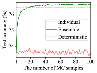
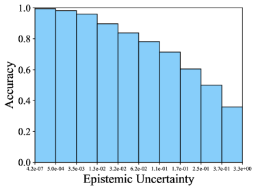
Figure 5: (Left): Test accuracy varies w.r.t. the number of MC samples for Bayes ensemble. (Right): Comparison on the accuracy for instance buckets of equal size but with rising uncertainty. (BayesAdapter (MFG), ImageNet)

The impact of ensemble number. We draw the change of test accuracy w.r.t. the number of MC samples $S$ for Bayes ensemble in Figure 5 (Left). The model is trained by BayesAdapter (MFG) on ImageNet. The points on the red line represent the individual accuracies of the 100 parameter samples. The yellow dashed line refers to the deterministic inference with only the Gaussian mean. The green line displays the effects of Bayes ensemble – the predictive performance increases from $<74\%$ to $>76\%$ quickly before seeing 20 parameter samples, and gradually saturates after that.

Uncertainty-based rejective decision. In practice, we expect our models to be accurate on the data that they are certain about. In this spirit, we gather the epistemic uncertainty estimates for ImageNet validation data given by BayesAdapter (MFG), based on which we divide the data into 10 buckets of equal size but with increasing uncertainty. We depict the average accuracy of each bucket in Figure 5 (Right). As expected, our BNN is more accurate for instances with smaller uncertainty.

5 Related Work

Fruitful works have emerged in the BNN community in the last decade (Graves, 2011; Welling and Teh, 2011; Blundell et al., 2015; Kingma and Welling, 2013; Balan et al., 2015; Liu and Wang, 2016; Kendall and Gal, 2017; Wu et al., 2018). However, most of the existing works cannot achieve the goal of practicability. For example, some works trade learning efficiency for flexible variational posteriors, leading to restrictive scalability (Louizos and Welling, 2016, 2017; Shi et al., 2018a; Sun et al., 2019). Khan et al. (2018); Zhang et al. (2018); Osawa et al. (2019) build Adam-like optimizers to do variational inference, but their parallel training throughput and compatibility with data augmentation are inferior to SGD. Approximate Bayesian methods like Monte Carlo dropout (Gal and Ghahramani, 2016) and Deep Ensemble (Lakshminarayanan et al., 2017) can maintain good predictive performance but suffer from degenerated uncertainty estimates (Fort et al., 2019) or high cost.

Laplace approximation (MacKay, 1992; Ritter et al., 2018) is a known approach to transform a DNN to a BNN, but it is inflexible due to its postprocessing nature and some strong assumptions made for practical concerns. Alternatively, BayesAdapter works in the style of fine-tuning, which is more natural and economical for deep networks. Bayesian modeling the last layer of a DNN is proposed recently (Kristiadi et al., 2020), and its combination with BayesAdapter deserves an investigation. BayesAdapter connects to MOPED (Krishnan et al., 2020) in that their variational configurations are both based on MAP. However, MOPED solves the prior specification problem for BNNs while BayesAdapter constitutes a practical framework to bring variational BNNs to the masses. In detail, MOPED uses MAP to define the prior while BayesAdapter uses MAP to initialize the parameters of the variational distribution. Beyond this, this work makes valuable technical contributions including the PSE variational and the refinement of exemplar reparameterization. We have also done a thorough study on how pre-training benefits VI. Moreover, the results in Appendix C show that MOPED suffers from more serious over-fitting than BayesAdapter.

6 Conclusion

This work proposes the BayesAdapter framework to ease the learning of variational BNNs. Our core idea is to perform Bayesian fine-tuning instead of expensive from-scratch Bayesian learning. We develop plug-and-play implementations for the stochastic variational inference under two representative variational distributions, and refine exemplar reparameterization to efficiently reduce gradient variance. We evaluate BayesAdapter in diverse scenarios and report promising results. One limitation of BayesAdapter is that practitioners may need to carefully tune the optimization configurations for Bayesian fine-tuning to achieve reasonable performance. Regarding future work, the application of BayesAdapter to more exciting scenarios like contextual bandits deserves further investigation.

References

- Balan et al. (2015) Anoop Korattikara Balan, Vivek Rathod, Kevin P Murphy, and Max Welling. Bayesian dark knowledge. In Advances in Neural Information Processing Systems, pages 3438–3446, 2015.
- Blundell et al. (2015) Charles Blundell, Julien Cornebise, Koray Kavukcuoglu, and Daan Wierstra. Weight uncertainty in neural network. In International Conference on Machine Learning, pages 1613–1622, 2015.
- Chetlur et al. (2014) Sharan Chetlur, Cliff Woolley, Philippe Vandermersch, Jonathan Cohen, John Tran, Bryan Catanzaro, and Evan Shelhamer. cudnn: Efficient primitives for deep learning. arXiv preprint arXiv:1410.0759, 2014.
- Daxberger et al. (2021) Erik Daxberger, Agustinus Kristiadi, Alexander Immer, Runa Eschenhagen, Matthias Bauer, and Philipp Hennig. Laplace redux-effortless bayesian deep learning. Advances in Neural Information Processing Systems, 34:20089–20103, 2021.
- Deng et al. (2009) J. Deng, W. Dong, R. Socher, L.-J. Li, K. Li, and L. Fei-Fei. ImageNet: A Large-Scale Hierarchical Image Database. In CVPR09, 2009.
- Deng et al. (2019) Jiankang Deng, Jia Guo, Niannan Xue, and Stefanos Zafeiriou. Arcface: Additive angular margin loss for deep face recognition. In Proceedings of the IEEE Conference on Computer Vision and Pattern Recognition, pages 4690–4699, 2019.
- Depeweg et al. (2016) Stefan Depeweg, José Miguel Hernández-Lobato, Finale Doshi-Velez, and Steffen Udluft. Learning and policy search in stochastic dynamical systems with Bayesian neural networks. arXiv preprint arXiv:1605.07127, 2016.
- Fort et al. (2019) Stanislav Fort, Huiyi Hu, and Balaji Lakshminarayanan. Deep ensembles: A loss landscape perspective. arXiv preprint arXiv:1912.02757, 2019.
- Gal and Ghahramani (2015) Yarin Gal and Zoubin Ghahramani. Dropout as a bayesian approximation: appendix. arXiv preprint arXiv:1506.02157, 420, 2015.
- Gal and Ghahramani (2016) Yarin Gal and Zoubin Ghahramani. Dropout as a Bayesian approximation: Representing model uncertainty in deep learning. In International Conference on Machine Learning, pages 1050–1059, 2016.
- Graves (2011) Alex Graves. Practical variational inference for neural networks. In Advances in Neural Information Processing Systems, pages 2348–2356, 2011.
- Guo et al. (2017) Chuan Guo, Geoff Pleiss, Yu Sun, and Kilian Q Weinberger. On calibration of modern neural networks. arXiv preprint arXiv:1706.04599, 2017.
- He et al. (2020) Bobby He, Balaji Lakshminarayanan, and Yee Whye Teh. Bayesian deep ensembles via the neural tangent kernel. arXiv preprint arXiv:2007.05864, 2020.
- He et al. (2016a) Kaiming He, Xiangyu Zhang, Shaoqing Ren, and Jian Sun. Deep residual learning for image recognition. In Proceedings of the IEEE Conference on Computer Vision and Pattern Recognition, pages 770–778, 2016a.
- He et al. (2016b) Kaiming He, Xiangyu Zhang, Shaoqing Ren, and Jian Sun. Identity mappings in deep residual networks. In European Conference on Computer Vision, pages 630–645, 2016b.
- Hendrycks and Dietterich (2019) Dan Hendrycks and Thomas Dietterich. Benchmarking neural network robustness to common corruptions and perturbations. arXiv preprint arXiv:1903.12261, 2019.
- Hernández-Lobato and Adams (2015) José Miguel Hernández-Lobato and Ryan Adams. Probabilistic backpropagation for scalable learning of Bayesian neural networks. In International Conference on Machine Learning, pages 1861–1869, 2015.
- Hron et al. (2018) Jiri Hron, Alex Matthews, and Zoubin Ghahramani. Variational bayesian dropout: pitfalls and fixes. In International Conference on Machine Learning, pages 2019–2028. PMLR, 2018.
- Huang et al. (2017) Gao Huang, Zhuang Liu, Laurens Van Der Maaten, and Kilian Q Weinberger. Densely connected convolutional networks. In Proceedings of the IEEE Conference on Computer Vision and Pattern Recognition, pages 4700–4708, 2017.
- Huang et al. (2007) Gary B Huang, Marwan Mattar, Tamara Berg, and Eric Learned-Miller. Labeled faces in the wild: A database forstudying face recognition in unconstrained environments. In Technical report, 2007.
- Kendall and Gal (2017) Alex Kendall and Yarin Gal. What uncertainties do we need in Bayesian deep learning for computer vision? In Advances in Neural Information Processing Systems, pages 5574–5584, 2017.
- Khan et al. (2018) Mohammad Emtiyaz Khan, Didrik Nielsen, Voot Tangkaratt, Wu Lin, Yarin Gal, and Akash Srivastava. Fast and scalable Bayesian deep learning by weight-perturbation in adam. In International Conference on Machine Learning, pages 2616–2625, 2018.
- Kingma and Welling (2013) Diederik P Kingma and Max Welling. Auto-encoding variational Bayes. arXiv preprint arXiv:1312.6114, 2013.
- Kingma et al. (2015) Durk P Kingma, Tim Salimans, and Max Welling. Variational dropout and the local reparameterization trick. In Advances in Neural Information Processing Systems, pages 2575–2583, 2015.
- Krishnan et al. (2020) Ranganath Krishnan, Mahesh Subedar, and Omesh Tickoo. Specifying weight priors in bayesian deep neural networks with empirical bayes. In Proceedings of the AAAI Conference on Artificial Intelligence, volume 34, pages 4477–4484, 2020.
- Kristiadi et al. (2020) Agustinus Kristiadi, Matthias Hein, and Philipp Hennig. Being bayesian, even just a bit, fixes overconfidence in relu networks. arXiv preprint arXiv:2002.10118, 2020.
- Krizhevsky et al. (2009) Alex Krizhevsky, Geoffrey Hinton, et al. Learning multiple layers of features from tiny images. 2009.
- Lakshminarayanan et al. (2017) Balaji Lakshminarayanan, Alexander Pritzel, and Charles Blundell. Simple and scalable predictive uncertainty estimation using deep ensembles. In Advances in Neural Information Processing Systems, pages 6402–6413, 2017.
- Leibig et al. (2017) Christian Leibig, Vaneeda Allken, Murat Seçkin Ayhan, Philipp Berens, and Siegfried Wahl. Leveraging uncertainty information from deep neural networks for disease detection. Scientific Reports, 7(1):1–14, 2017.
- Li and Turner (2017) Yingzhen Li and Richard E Turner. Gradient estimators for implicit models. arXiv preprint arXiv:1705.07107, 2017.
- Liu and Wang (2016) Qiang Liu and Dilin Wang. Stein variational gradient descent: A general purpose Bayesian inference algorithm. In Advances in Neural Information Processing Systems, pages 2378–2386, 2016.
- Louizos and Welling (2016) Christos Louizos and Max Welling. Structured and efficient variational deep learning with matrix gaussian posteriors. In International Conference on Machine Learning, pages 1708–1716, 2016.
- Louizos and Welling (2017) Christos Louizos and Max Welling. Multiplicative normalizing flows for variational Bayesian neural networks. In International Conference on Machine Learning, pages 2218–2227, 2017.
- MacKay (1992) David JC MacKay. A practical Bayesian framework for backpropagation networks. Neural Computation, 4(3):448–472, 1992.
- Maddox et al. (2019) Wesley J Maddox, Pavel Izmailov, Timur Garipov, Dmitry P Vetrov, and Andrew Gordon Wilson. A simple baseline for bayesian uncertainty in deep learning. In Advances in Neural Information Processing Systems, pages 13153–13164, 2019.
- Neal (1995) Radford M Neal. Bayesian Learning for Neural Networks. PhD thesis, University of Toronto, 1995.
- Netzer et al. (2011) Yuval Netzer, Tao Wang, Adam Coates, Alessandro Bissacco, Bo Wu, and Andrew Y Ng. Reading digits in natural images with unsupervised feature learning. 2011.
- Osawa et al. (2019) Kazuki Osawa, Siddharth Swaroop, Anirudh Jain, Runa Eschenhagen, Richard E Turner, Rio Yokota, and Mohammad Emtiyaz Khan. Practical deep learning with Bayesian principles. arXiv preprint arXiv:1906.02506, 2019.
- Paszke et al. (2019) Adam Paszke, Sam Gross, Francisco Massa, Adam Lerer, James Bradbury, Gregory Chanan, Trevor Killeen, Zeming Lin, Natalia Gimelshein, Luca Antiga, et al. Pytorch: An imperative style, high-performance deep learning library. In Advances in neural information processing systems, pages 8026–8037, 2019.
- Ritter et al. (2018) Hippolyt Ritter, Aleksandar Botev, and David Barber. A scalable laplace approximation for neural networks. In 6th International Conference on Learning Representations, ICLR 2018-Conference Track Proceedings, volume 6. International Conference on Representation Learning, 2018.
- Sandler et al. (2018) Mark Sandler, Andrew Howard, Menglong Zhu, Andrey Zhmoginov, and Liang-Chieh Chen. Mobilenetv2: Inverted residuals and linear bottlenecks. In Proceedings of the IEEE conference on computer vision and pattern recognition, pages 4510–4520, 2018.
- Sengupta et al. (2016) Soumyadip Sengupta, Jun-Cheng Chen, Carlos Castillo, Vishal M Patel, Rama Chellappa, and David W Jacobs. Frontal to profile face verification in the wild. In 2016 IEEE Winter Conference on Applications of Computer Vision (WACV), pages 1–9. IEEE, 2016.
- Shi et al. (2018a) Jiaxin Shi, Shengyang Sun, and Jun Zhu. Kernel implicit variational inference. In International Conference on Learning Representations, 2018a.
- Shi et al. (2018b) Jiaxin Shi, Shengyang Sun, and Jun Zhu. A spectral approach to gradient estimation for implicit distributions. arXiv preprint arXiv:1806.02925, 2018b.
- Smith and Gal (2018) Lewis Smith and Yarin Gal. Understanding measures of uncertainty for adversarial example detection. arXiv preprint arXiv:1803.08533, 2018.
- Sun et al. (2019) Shengyang Sun, Guodong Zhang, Jiaxin Shi, and Roger Grosse. Functional variational Bayesian neural networks. In International Conference on Learning Representations, 2019.
- Vaswani et al. (2017) Ashish Vaswani, Noam Shazeer, Niki Parmar, Jakob Uszkoreit, Llion Jones, Aidan N Gomez, Łukasz Kaiser, and Illia Polosukhin. Attention is all you need. In Advances in neural information processing systems, pages 5998–6008, 2017.
- Welling and Teh (2011) Max Welling and Yee W Teh. Bayesian learning via stochastic gradient langevin dynamics. In Proceedings of the 28th international conference on machine learning (ICML-11), pages 681–688, 2011.
- Wen et al. (2018) Yeming Wen, Paul Vicol, Jimmy Ba, Dustin Tran, and Roger Grosse. Flipout: Efficient pseudo-independent weight perturbations on mini-batches. arXiv preprint arXiv:1803.04386, 2018.
- Wen et al. (2020) Yeming Wen, Dustin Tran, and Jimmy Ba. Batchensemble: an alternative approach to efficient ensemble and lifelong learning. arXiv preprint arXiv:2002.06715, 2020.
- Wenzel et al. (2020a) Florian Wenzel, Kevin Roth, Bastiaan S Veeling, Jakub Swiatkowski, Linh Tran, Stephan Mandt, Jasper Snoek, Tim Salimans, Rodolphe Jenatton, and Sebastian Nowozin. How good is the bayes posterior in deep neural networks really? arXiv preprint arXiv:2002.02405, 2020a.
- Wenzel et al. (2020b) Florian Wenzel, Jasper Snoek, Dustin Tran, and Rodolphe Jenatton. Hyperparameter ensembles for robustness and uncertainty quantification. arXiv preprint arXiv:2006.13570, 2020b.
- Wilson and Izmailov (2020) Andrew Gordon Wilson and Pavel Izmailov. Bayesian deep learning and a probabilistic perspective of generalization. arXiv preprint arXiv:2002.08791, 2020.
- Wu et al. (2018) Anqi Wu, Sebastian Nowozin, Edward Meeds, Richard E Turner, Jose Miguel Hernandez-Lobato, and Alexander L Gaunt. Deterministic variational inference for robust bayesian neural networks. arXiv preprint arXiv:1810.03958, 2018.
- Yi et al. (2014) Dong Yi, Zhen Lei, Shengcai Liao, and Stan Z Li. Learning face representation from scratch. arXiv preprint arXiv:1411.7923, 2014.
- Zagoruyko and Komodakis (2016) Sergey Zagoruyko and Nikos Komodakis. Wide residual networks. arXiv preprint arXiv:1605.07146, 2016.
- Zhang et al. (2018) Guodong Zhang, Shengyang Sun, David Duvenaud, and Roger Grosse. Noisy natural gradient as variational inference. In International Conference on Machine Learning, pages 5847–5856, 2018.
- Zheng and Deng (2018) Tianyue Zheng and Weihong Deng. Cross-pose lfw: A database for studying cross-pose face recognition in unconstrained environments. Beijing University of Posts and Telecommunications, Tech. Rep, 5, 2018.
- Zheng et al. (2017) Tianyue Zheng, Weihong Deng, and Jiani Hu. Cross-age lfw: A database for studying cross-age face recognition in unconstrained environments. arXiv preprint arXiv:1708.08197, 2017.