Channel Prediction for mmWave Ground-to-Air Propagation under Blockage

Abstract

Ground-to-air (GA) communication using unmanned aerial vehicles (UAVs) has gained popularity in recent years and is expected to be part of 5G networks and beyond. However, the GA links are susceptible to frequent blockages at millimeter wave (mmWave) frequencies. During a link blockage, the channel information cannot be obtained reliably. In this work, we provide a novel method of channel prediction during the GA link blockage at $28$ GHz. In our approach, the multipath components (MPCs) along a UAV flight trajectory are arranged into independent path bins based on the minimum Euclidean distance among the channel parameters of the MPCs. After the arrangement, the channel parameters of the MPCs in individual path bins are forecasted during the blockage. An autoregressive model is used for forecasting. The results obtained from ray tracing simulations indicate a close match between the actual and the predicted mmWave channel.

I Introduction

The use of civilian unmanned aerial vehicles (UAVs) for everyday applications have seen a surge in recent years such as surveillance, video recording, search and rescue, and hot spot communications. However, the UAV ground-to-air (GA) communication links are susceptible to blockages due to high rise buildings or trees. These blockages are significant at millimeter wave (mmWave) frequencies compared to sub-6 GHz frequencies. Channel prediction can be used to predict the state of the channel during blockages and improve link reliability, which has not been studied in the literature for GA scenarios to our best knowledge.

The literature for channel prediction can be divided into three main categories. 1) Autoregressive (AR) model based methods [1, 2], 2) Sum of sinusoids (SoS) [3, 4], and basis expansion models (BEM) [5, 6], and 3) Artificial intelligence (AI) based models [7, 8, 9]. AR based prediction methods are the most popular, frequently used, and computationally simple, but their accuracy suffers in fast and complicated varying channels. The SoS methods require rigorous channel prediction calculations over short time durations for fast varying channels that become computationally not feasible for real-time environments and are therefore mostly used for simulated environments. The computational complexity and accuracy for the BEM are dependent on the type of the basis function and the type of the channel. The AI based recurrent neural networks (RNN) have gained popularity in recent years for channel prediction [7], which have a high computational load for the training at regular intervals, as they require large memory and data for fast varying channels and complex environments. Channel prediction aided with the 3D maps of the urban propagation environment [10, 11], are also available in the literature. For example, in [12, 13], the prediction of signal strength for trajectory planning of relay UAVs is aided with the help of maps. Comprehensive 3D data is required for the whole environment for map aided channel prediction methods. Also, the prediction accuracy suffers if the maps are outdated and real-time environmental variations are not included in the maps.

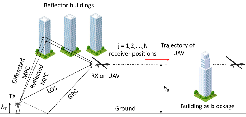
Figure 1: The UAV GA propagation scenario with blockage.

In this work, we have introduced a novel channel prediction method for GA communication links. The GA propagation scenario for our work is shown in Fig. 1. Our approach can be divided into two parts. In the first part, an Euclidean distance (ED) based algorithm is used, which arranges the MPCs obtained along the UAV trajectory into individual path bins. The arrangement is based on a minimum ED among the channel parameters of the MPCs, and it results in a trend of individual channel parameters of MPCs in a path bin. In the second part, the trend of individual channel parameters in a path bin is used to forecast the channel parameters during the blockage. The forecasting is performed using an auto-regressive (AR) model. The simulations are carried out using the Wireless InSite ray tracing software. The results indicate that the actual and the forecasted channel parameters are close. We also provide a distance-based prediction approach for the death of a path bin along the UAV trajectory, and performance comparison with other popular prediction methods.

II System Model

We consider a GA propagation scenario shown in Fig. 1. The transmitter (TX) is on the ground and the receiver (RX) is on a UAV. The height of the TX and RX above the ground is $h_{\rm T}$ and $h_{\rm R}$, respectively. The received MPCs in Fig. 1 are categorized as: i) line-of-sight (LOS), ii) ground reflected component (GRC), and iii) reflected and/or diffracted from scatterers. We consider six channel parameters of each MPC: two in the temporal and four in the spatial domain.

II-A Euclidean Distance of MPCs’ Channel Parameters

Let $H(n)$ represent the time-varying channel impulse response of the system. Then, we may write

$$\big{|}H(n)\big{|}^{2}=\sum_{m=1}^{M}\big{|}\alpha_{m}(n)\big{|}^{2}\delta\big{(}n-\tau_{m}(n)\big{)}\delta\big{(}\vv{\boldsymbol{\Theta}}^{\rm(TX)}-\theta_{m}^{\rm(TX)}$$

$$\delta\big{(}\vv{\boldsymbol{\Phi}}^{\rm(TX)}-\phi_{m}^{\rm(TX)}\big{)}\delta\big{(}\vv{\boldsymbol{\Theta}}^{\rm(RX)}-\theta_{m}^{\rm(RX)}\big{)}\delta\big{(}\vv{\boldsymbol{\Phi}}^{\rm(RX)}-\phi_{m}^{\rm(RX)}\big{)},$$ (1)

where $n$ is the time instance, $M$ is the total number of MPCs, $\alpha_{m}(n)$, $\tau_{m}(n)$ represents the complex amplitude and delay of the $m^{\rm th}$ MPC, respectively, $\vv{\boldsymbol{\Theta}}^{(\rm TX)},\vv{\boldsymbol{\Phi}}^{(\rm TX)}$ are the angle of departure (AoD) vectors in the elevation and azimuth planes, respectively, $\vv{\boldsymbol{\Theta}}^{(\rm RX)},\vv{\boldsymbol{\Phi}}^{(\rm RX)}$ are AoA vectors in the elevation and azimuth planes, respectively, and the AoD and AoA of the $m^{\rm th}$ MPC in the elevation and azimuth planes respectively, are represented as $\theta_{m}^{\rm(TX)}$, $\phi_{m}^{\rm(TX)}$, $\theta_{m}^{\rm(RX)}$, $\phi_{m}^{\rm(RX)}$.

From (1), if $P_{\rm T}$ is the transmitted power, the total received power $P_{\rm R}$ at a RX position is given as

$$P_{\rm R} =\frac{P_{\rm T}\lambda^{2}}{(4\pi)^{2}}\bigg{[}\frac{G^{(\rm TX)}\big{(}\theta_{1},\phi_{1}\big{)}G^{(\rm RX)}\big{(}\theta_{1},\phi_{1}\big{)}}{R_{1}^{2}}+$$ (2)

$$\frac{\sum_{s=0}^{S}\sum_{m=1}^{M_{s}}G^{(\rm TX)}\big{(}\theta_{s,m},\phi_{s,m}\big{)}G^{(\rm RX)}\big{(}\theta_{s,m},\phi_{s,m}\big{)}\Gamma_{s,m}}{R_{s,m}^{2}}\bigg{]},$$

where the first term is for the LOS and the second term represents the MPCs from scatterers, $\lambda$ is the wavelength, $G^{(\rm TX)}\big{(}\theta,\phi\big{)}$ and $G^{(\rm RX)}\big{(}\theta,\phi\big{)}$ are the antenna gains at the TX and RX, respectively, at elevation angle $\theta$ and azimuth angle $\phi$, $\Gamma_{s,m}$ is the reflection coefficient, and $R_{s,m}$ is the total distance traveled by the $m^{\rm th}$ MPC due to interaction with the $s^{\rm th}$ scatterer, and the distance of the LOS path is represented as $R_{1}$. Moreover, the total number of scatterers are $S$ and the total number of MPCs due to a scatterer is represented as $M_{s}$.

Algorithm 1 Arrangement of MPCs into path bins.

1:procedure Pathbins

2:Initialize each path bin with the MPC at first RX position

3:% At the $j^{\rm th}$ RX position and from (4) and (5), the ED is

4:    for $m=1:M_{j}$ do % MPCs at $j^{\rm th}$ RX position

5:         for $i=j-1:1$ do  % previous

6:             for $k=1:M_{i}$ do  % MPCs at previous

7:                 Calculate $d(j,m,i,k)$

8:             end for

9:         end for

10:         $d_{\rm min}(m)$ = $\displaystyle\min_{\forall i,k}d$

11:         if $d_{\rm min}(m)<\epsilon$ then

12:             for $l=1$:Number of path bins do

13:                 (i) Select min$(d_{l})$, and,

14:                 (ii) add the $m^{\rm th}$ MPC at $j^{\rm th}$ RX position to $l^{\rm th}$

15:                 path bin. % MPCs placement in a path bin

16:             end for

17:         end if

18:         if $d_{\rm min}(m)>\epsilon$ then

19:             (i) Birth of a new MPC and a path bin, and,

20:             (ii) temporary discontinuation of a path bin

21:         end if

22:    end for

23:    if $M_{j}<M_{j-1}$ then

24:         (i) Death of a MPC, and,

25:         (ii) temporary discontinuation of corresponding path bin

26:    end if

27:return path bins

28:end procedure

From Fig. 1, the RX positions along the UAV trajectory are labeled as $j=1,2,...,N$. At a $j^{\rm th}$ RX position and $m^{\rm th}$ MPC, a MPC vector represented as $\vv{\textbf{MC}}_{j,m}$ is given by:

$$\vv{\textbf{MC}}_{j,m}=\big{[}\alpha_{j,m},\tau_{j,m},\theta_{j,m}^{(\rm TX)},\phi_{j,m}^{(\rm TX)},\theta_{j,m}^{(\rm RX)},\phi_{j,m}^{(\rm RX)}\big{]}.$$ (3)

The MPCs till the $(j-1)^{\rm th}$ RX position are given by:

$$\begin{bmatrix}\vv{\textbf{MC}}_{1,1}&\vv{\textbf{MC}}_{1,2}&\vv{\textbf{MC}}_{1,3}&\cdots&\vv{\textbf{MC}}_{1,M_{1}}\\ \vv{\textbf{MC}}_{2,1}&\vv{\textbf{MC}}_{2,2}&\vv{\textbf{MC}}_{2,3}&\cdots&\vv{\textbf{MC}}_{2,M_{2}}\\ \vdots&\vdots&\vdots&\cdots&\vdots\\ \vv{\textbf{MC}}_{j-1,1}&\vv{\textbf{MC}}_{j-1,2}&\vv{\textbf{MC}}_{j-1,3}&\cdots&\vv{\textbf{MC}}_{j-1,M_{j-1}}\end{bmatrix}~{},$$

which is used to calculate the ED of a MPC at $j^{\rm th}$ RX position with the MPCs at RX positions $[j-1,j-2,\ldots,1]$. The number of previous RX positions for ED calculation can be varied to reduce the channel data. The ED between the channel parameters of the $m^{\rm th}$ MPC at $j^{\rm th}$ RX position and the channel parameters of $k^{\rm th}$ MPC at $i^{\rm th}$ RX position, where $i=j-1,j-2,\ldots,1$, is given by:

$$d^{(v)}(j,m,i,k)={\rm Euclidean}\big{(}\vv{\textbf{MC}}_{j,m}(v),\vv{\textbf{MC}}_{i,k}(v)\big{)}~{},$$ (4)

where $v=1,2,...,6$ refers to the six channel parameters of a MPC as in (3). The total ED of the $m^{\rm th}$ MPC at $j^{\rm th}$ RX position, from the $k^{\rm th}$ MPC at $i^{\rm th}$ RX position is given by

$$d(j,m,i,k)=\frac{1}{\gamma}\sum_{v=1}^{6}d^{(v)}(j,m,i,k)~{},$$ (5)

where $\gamma$ is the normalizing factor. The value of $\gamma$ can vary from $1$ to $\max\big{(}\sum_{v=1}^{6}d^{(v)}(j,m,i,k)\big{)}~{}\forall~{}j,m,i,k$.

II-B Channel Prediction Algorithms

The pseudocode for arranging the MPCs in path bins is shown in Algorithm 1, where two minimum ED conditions are used for a MPC to be placed in a path bin. The first condition takes the distance of the $m^{\rm th}$ MPC at a $j^{\rm th}$ RX position with the MPCs at previous RX positions. The distance is calculated among individual channel parameters of MPCs represented from $d^{(1)}$ to $d^{(6)}$ in (4). The distance of individual channel parameters are added and normalized by $\gamma$ to get $d$ in (5). In Algorithm 1, the minimum value of $d$ for the $m^{\rm th}$ MPC is compared with the threshold $\epsilon$, given as $d_{\rm min}(m)<\epsilon$. If this condition is true, the MPC is selected and a second minimum distance condition is applied. In the second condition, min$(d_{l})$ is used, where $d_{l}$ is the ED of selected MPC with the existing MPCs in the $l^{\rm th}$ path bin. This condition selects the $l^{\rm th}$ path bin, where the MPC will be placed. The minimum distance, $d_{\rm min}$ threshold, $\epsilon$ in Algorithm 1 is dependent on the normalizing factor $\gamma$.

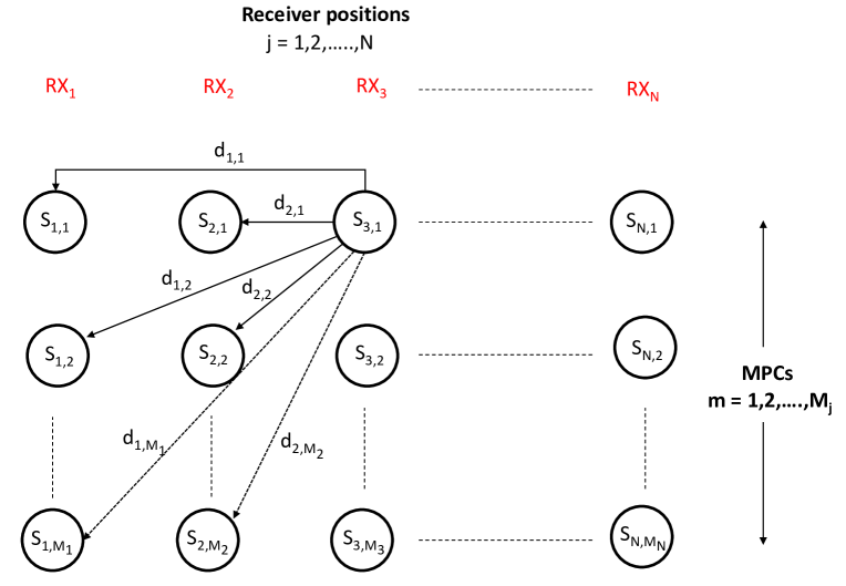
Figure 2: A Markov chain model based on the minimum ED.

Algorithm 2 Forecasting of the channel parameters in path bins during blockage.

1:procedure Forecasting(path bins)

2:Let $\vv{\textbf{MC}}_{{pb}_{1}}$ represent the MPCs in the first path bin $\vv{\textbf{PB}}_{1}$, and $pb_{1}=1,2,...,M_{{pb}_{1}}$, where $M_{{pb}_{1}}$ is the total number of MPCs in $\vv{\textbf{PB}}_{1}$ over all the

3:The six channel parameters of the MPCs in $\vv{\textbf{PB}}_{1}$ from (3) are represented as $\vv{\textbf{MC}}_{{pb}_{1}}(v)$,  $v=1,2,...,6$

4:Fit an $n^{\rm th}$ order AR model to a channel parameter $\vv{\textbf{MC}}_{{pb}_{1}}(v)$ obtained over RX positions as

5:    $S_{\rm AR}$ = AR($\vv{\textbf{MC}}_{{pb}_{1}}(v)$, $n$)

6:If $K^{\rm(fc)}$ are the number of points to be forecasted, then the forecasted data $\vv{\textbf{MC}}_{{pb}_{1}}^{(\rm fc)}(v)$, based on system model $S_{\rm AR}$ and past data $\vv{\textbf{MC}}_{{pb}_{1}}(v)$ is

7:    $\vv{\textbf{MC}}_{{pb}_{1}}^{(\rm fc)}(v)$ = $\rm{forecast}$($S_{\rm AR}$,  $\vv{\textbf{MC}}_{{pb}_{1}}(v)$,  $K^{\rm(fc)}\big{)}$

8:return $\vv{\textbf{MC}}_{{pb}_{1}}^{(\rm fc)}(v)$

9:end procedure

From Algorithm 1, if $d_{\rm min}(m)>\epsilon$, the similarity criteria for the $m^{\rm th}$ MPC with any of the MPCs at previous RX positions is not met. Therefore, this MPC is considered a new MPC (birth), and a new path bin is created for it. Moreover, if the number of MPCs at $j^{\rm th}$ RX position is less than the $(j-1)^{\rm th}$ position, this indicates the death of a MPC. In both the above conditions, one of the existing path bins will be discontinued. This discontinuation can be temporary as these path bins can continue (resurrect) at a later part of the UAV trajectory. The value of $\gamma$ in (5) and $\epsilon$ in Algorithm 1 is $75.8$ and $0.15$, respectively.

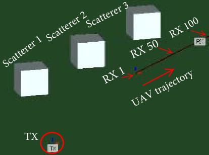
Figure 3: 28 GHz simulation scenario in Wireless InSite ray tracing software.

From Algorithm 1, the transition of MPCs along the RX positions based on ED in a path bin can be modeled using a Markov chain. A transition likelihood scenario based on the Markov chain for the first MPC at the third RX position is shown in Fig. 2. The state of a Markov chain at $j^{\rm th}$ RX position and $m^{\rm th}$ MPC is represented as $S_{j,m}$. The transition among the states is dependent on the minimum ED. The minimum transition distance in Fig. 2 will determine which path bin the first MPC at the third RX position will occupy. Therefore, an $l^{\rm th}$ path bin from Algorithm 1 is represented as a sequence of selected Markov states along the RX positions. Algorithm 1 can handle any UAV trajectory. A change in the UAV trajectory is accompanied by the birth and death of MPCs that will be tracked and updated by Algorithm 1.

TABLE I: Parameters for ray tracing simulations.

Parameter	Parameter value
Center frequency	$28$ GHz
Antenna radiation pattern (azimuth)	Omnidirectional
Antenna polarization	Vertical
Height of TX, $h_{\rm T}$	$2$ m
Height of RX (on UAV), $h_{\rm R}$	$50$ m
Length of UAV trajectory	$100$ m
Distance of TX to start of trajectory	$243$ m
Horizontal scatterer distance from trajectory	$145$ m
Dimension of scatterers	40 m$\times$40 m$\times$ 40 m
Distance among scatterers	$110$ m
Permittivity of ground	$3.5$
Permittivity of scatterer structure	$5.31$

The placement of MPCs with similar channel characteristics in path bins results in a trend of individual channel parameters along the UAV trajectory. In case of a blockage, the trend of a channel parameter in a path bin is used to forecast it. Our approach for forecasting the channel parameters is given in Algorithm 2, where the individual channel parameters in a path bin form a time series. An $n^{\rm th}$ order AR model is fitted to individual channel parameters. The time series system model using autoregression is represented as $S_{\rm AR}$ in Algorithm 2. The forecasting over $K^{(\rm fc)}$ future steps is performed using a system model and past channel parameter data.

III Simulation Scenario and Results

The simulations are carried out using the Wireless InSite ray tracing software (see Fig. 3 and Table I). Fig. 4 shows the received power of the MPCs along the RX positions. The MPCs are positioned based on descending received power at respective RX positions. For example, in the start of Fig. 4 at RX position 1, there are five MPCs. The LOS and GRC (with larger received power compared to other MPCs) occupy the first and second positions, respectively, followed by the other MPCs. However, from Fig. 4, no clear pattern of received power of the MPCs over the RX positions can be observed, except for the LOS path. Also, we cannot differentiate the birth, and death of the MPCs along the RX positions.

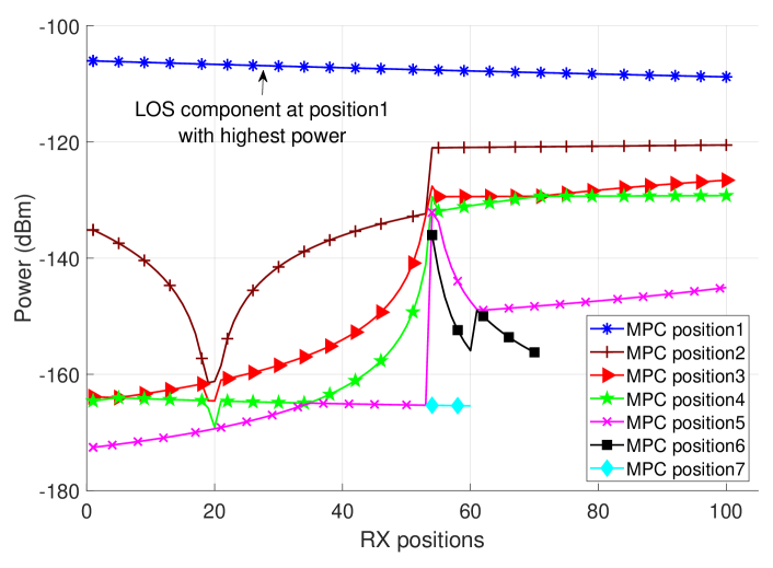
Figure 4: Power of received MPCs along the UAV trajectory without applying Algorithm 1. The MPCs are positioned based on descending received power.

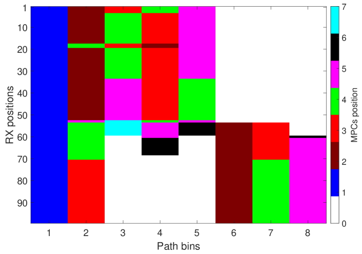
Figure 5: Position of the MPCs in individual path bins, sequenced using Algorithm 1. For example, the LOS path is shown in path bin $1$.

III-A MPC Identification and Channel Gain Prediction

The selected MPCs (or states in Fig. 2) from Algorithm 1, are placed in the respective path bins. The arrangement of the MPCs in path bins at RX positions is shown in Fig. 5. Compared to Fig. 4, the MPCs in Fig. 5 are placed in individual path bins based on the similarity of the channel parameters. Moreover, the number of path bins is controlled by the similarity criteria set by $\epsilon$ in Algorithm 1. Fig. 6 shows the received power of the MPCs in path bins after using Algorithm 1. A clear trend of the received power of the MPCs is observed in Fig. 6, as opposed to the results in Fig. 4. This trend is used for forecasting the received power during the blockage. The birth and death of the MPCs in Fig. 6 can also be identified. In addition, the trend of the received power of MPCs in Fig. 6 is used to predict the death of the MPCs in Section III-B. The trend of the other five channel parameters can be shown in a similar way.

A blockage is now considered at RX position 75. All the paths from RX position 75 onwards are removed. The channel parameters of the MPCs in path bins after RX position 75 are forecasted using Algorithm 2, that uses a Matlab based fourth-order AR model and forecast function. The forecasted power of the MPCs in path bins is shown in Fig. 7. Comparing Fig. 7 and Fig. 6, we observe that the forecasted and actual values are close and the mean square error (MSE) between the two is given in Table II. The other channel parameters are also forecasted during blockage in a similar way.

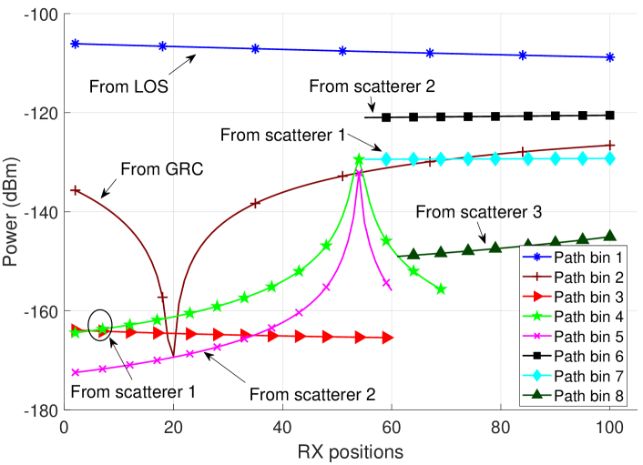
Figure 6: Received power of MPCs sequenced in individual path bins using Algorithm 1. The LOS and source of the MPCs in path bins are also provided.

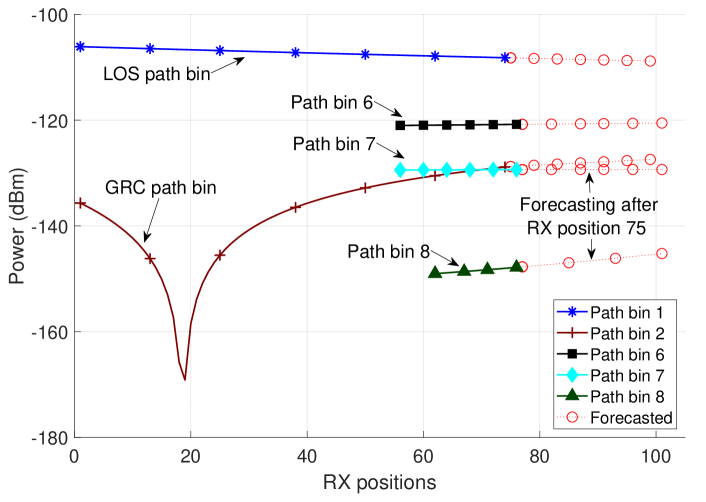
Figure 7: Forecasting received power of MPCs in path bins during the blockage.

III-B Prediction of Death of MPCs

From Fig. 6, we can observe the birth and death of the MPCs and corresponding path bins. We can also predict the death of a path bin (containing a resolvable MPC sequence) using Fig. 2. Let us take the LOS as the reference and denote the number of RX positions where the $l^{\rm th}$ path bin (from Algorithm 1) is not empty as $N_{l}$. Then, the average distance between the channel parameters of the $l^{\rm th}$ path bin and the LOS over $N_{l}$ RX positions is represented as $d_{l}=\sum_{i=j}^{N_{l}+j}\frac{d(i,l,i,1)}{N_{l}}$, using (5). The distance $d_{l}$ can be used to predict the death of the $l^{\rm th}$ path bin along the RX positions, where $l=2,3,...,8$, for the seven path bins, excluding the LOS. The greater the distance $d_{l}$, the greater the likelihood of the death of the $l^{\rm th}$ path bin. For the seven path bins in Fig. 5, $d_{l}=[0.68,5.07,4.29,4.45,3.85,4.01,4.18]$. If a distance threshold of $4.20$ is used, then path bins $3$, $4$, and $5$ with average distances greater than the threshold are predicted to die. This can also be observed in Fig. 6, where the received power of path bins is shown. A general observation can be drawn that the farther the channel parameters of a path bin from the channel parameters of the LOS over the RX positions, the greater the likelihood that the path bin will die.

A comparison of our approach with AR and long short-term memory RNN based prediction is provided in Table II. Our approach has higher accuracy compared to the other two methods due to accurate tracking/clustering of MPCs into respective path bins, which comes at the expense of increased computational complexity. The computational complexity for our approach consists mainly of distance calculation provided in Algorithm 1, and forecasting using AR model given in Algorithm 2. The computational complexity of RNN in Table II is obtained from [14], where $n_{\rm c}$ represents the number of memory cells. Overall, our approach can help to identify spur MPCs [15], estimate the number of scatterers in the environment, observe the birth, death, survival, resurrection, and trend of evolution of MPCs along the UAV trajectory in practical environments.

TABLE II: Comparison of our approach with popular prediction methods.

Predictor	Computational complexity	MSE [dB]	Stages	MAPE
This work	$O\Big{[}\big{(}6(N-1)M^{2}\big{)}^{2}+6nNM\Big{]}$	9.56	2	2.25%
AR model	$6nNM$	17.4	1	38.5%
RNN	O[4$n_{\rm c}^{2}$+30$NMn_{\rm c}$+3$n_{\rm c}$]	16	2	31.6%

IV Concluding Remarks

In this work, we have introduced a novel channel prediction method during GA link blockages. This method uses a ED based algorithm for arranging the MPCs into path bins. The arrangement places the MPCs with similar channel characteristics in individual path bins. The channel parameters of the MPCs in path bins are then forecasted during a link blockage with high accuracy. A distance-based prediction for the death of a MPC sequence is also provided.

References

- [1] A. Duel-Hallen, “Fading channel prediction for mobile radio adaptive transmission systems,” Proc. of the IEEE, vol. 95, no. 12, pp. 2299–2313, 2007.
- [2] A. Arredondo, K. R. Dandekar, and Guanghan Xu, “Vector channel modeling and prediction for the improvement of downlink received power,” IEEE Trans. Communs., vol. 50, no. 7, pp. 1121–1129, 2002.
- [3] R. Vaughan, P. Teal, and R. Raich, “Short-term mobile channel prediction using discrete scatterer propagation model and subspace signal processing algorithms,” in Proc. IEEE Vehic. Technol. Conf., vol. 2, Boston, MA, Sep. 2000, pp. 751–758.
- [4] M. Chen, T. Ekman, and M. Viberg, “New approaches for channel prediction based on sinusoidal modeling,” EURASIP Journal on Advances in Signal Processing, vol. 2007, pp. 1–13, 2006.
- [5] Z. Tang, R. C. Cannizzaro, G. Leus, and P. Banelli, “Pilot-assisted time-varying channel estimation for OFDM systems,” IEEE Trans. Signal Processing, vol. 55, no. 5, pp. 2226–2238, 2007.
- [6] T. Hrycak, S. Das, G. Matz, and H. G. Feichtinger, “Practical estimation of rapidly varying channels for OFDM systems,” IEEE Trans. Communs., vol. 59, no. 11, pp. 3040–3048, 2011.
- [7] W. Jiang and H. D. Schotten, “Neural network-based fading channel prediction: A comprehensive overview,” IEEE Access, vol. 7, pp. 118 112–118 124, 2019.
- [8] T. Ding and A. Hirose, “Online regularization of complex-valued neural networks for structure optimization in wireless-communication channel prediction,” IEEE Access, vol. 8, pp. 143 706–143 722, 2020.
- [9] T. Ding and A. Hirosse, “Fading channel prediction based on combination of complex-valued neural networks and chirp Z-transform,” IEEE Trans. Neural Networks and Learning Systems, vol. 25, no. 9, pp. 1686–1695, 2014.
- [10] E. K. Tameh, A. R. Nix, and M. A. Beach, “A 3-D integrated macro and microcellular propagation model, based on the use of photogrammetric terrain and building data,” in Proc. IEEE Vehic. Technol. Conf., vol. 3, Phoenix, AZ, May 1997, pp. 1957–1961.
- [11] E. Krijestorac, S. Hanna, and D. Cabric, “Spatial signal strength prediction using 3D maps and deep learning,” arXiv preprint arXiv:2011.03597, 2020.
- [12] P. Ladosz, H. Oh, and W. Chen, “Prediction of air-to-ground communication strength for relay UAV trajectory planner in urban environments,” in Proc. IEEE Int. Conf. on Intelligent Robots and Systems (IROS), 2017, pp. 6831–6836.
- [13] P. Ladosz, H. Oh, G. Zheng, and W. Chen, “A hybrid approach of learning and model-based channel prediction for commun. relay UAVs in dynamic urban environments,” IEEE Robotics and Automation Letters, vol. 4, no. 3, pp. 2370–2377, 2019.
- [14] H. Sak, A. W. Senior, and F. Beaufays, “Long short-term memory recurrent neural network architectures for large scale acoustic modeling,” 2014.
- [15] F. Erden, O. Ozdemir, W. Khawaja, and I. Guvenc, “Correction of channel sounding clock drift and antenna rotation effects for mmWave angular profile measurements,” IEEE Open Journal of Ant. and Propag., vol. 1, pp. 71–87, 2020.