On Stein rational balls smoothly but not symplectically embedded in $\mathbb{CP}^{2}$

Abstract.

We extend recent work of Brendan Owens by constructing a doubly infinite family of Stein rational homology balls which can be smoothly but not symplectically embedded in $\mathbb{CP}^{2}$.

1. Introduction and statement of results

Let $p>q\geq 1$ be coprime integers and $B_{p,q}$ the rational homology ball smoothing of the quotient singularity $\frac{1}{p^{2}}(pq-1,1)$. Using results by Khodorovskiy [4] it is not hard to show [1, § 2.1] that if the positive integers $p_{1}$, $p_{2}$ and $p_{3}$ form a Markov triple, that is $p_{1}^{2}+p_{2}^{2}+p_{3}^{2}=3p_{1}p_{2}p_{3}$, then there are pairwise disjoint symplectic embeddings

(1.1) $$B_{p_{i},q_{i}}\subset\mathbb{CP}^{2},\quad i=1,2,3,$$

where $q_{i}=\pm 3p_{j}/p_{k}\bmod p_{i}$ with $\{i,j,k\}=\{1,2,3\}$. Note that the sign is irrelevant because $B_{p,q}$ is symplectomorphic to $B_{p,p-q}$ [1, Remark 2.8]. The existence of the simultaneous symplectic embeddings (1.1) comes from the fact that when $(p_{1},p_{2},p_{3})$ is a Markov triple there is a $\mathbb{Q}$-Gorenstein smoothing to $\mathbb{CP}^{2}$ of the weighted projective space $\mathbb{CP}(p_{1}^{2},p_{2}^{2},p_{3}^{2})$. It is not possible to construct more than three disjoint symplectic embeddings using smoothings of singular surfaces. In fact, Hacking and Prokhorov [3] showed if $X$ is a projective surface with quotient singularities which has a $\mathbb{CP}^{2}$ smoothing, then $X$ is a $\mathbb{Q}$-Gorenstein deformation of such a weighted projective plane. Evans and Smith [1, Theorem 1.2] generalized this result to the symplectic category, showing that if $B_{p_{i},q_{i}}\subset\mathbb{CP}^{2}$, $i=1,...,N$ is a collection of pairwise disjoint symplectic embeddings then $N\leq 3$, the $p_{i}$ belong to Markov triples and the $q_{i}$’s must satisfy certain constraints. In particular, if $B_{p,q}\subset\mathbb{CP}^{2}$ is a symplectic embedding then $p$ must belong to a Markov triple and divide $q^{2}+9$.

Owens [9, Theorem 1] recently proved the existence of smooth embeddings

$$B_{F_{2n+1},F_{2n-1}}\subset\mathbb{CP}^{2}$$

for each $n\geq 1$, where $F_{2n-1}$ denotes the odd Fibonacci number, recursively defined by

$$F_{1}=1,\ F_{3}=2,\ F_{2n+3}=3F_{2n+1}-F_{2n-1}.$$

Moreover, he showed that the pair $(F_{2n+1},F_{2n-1})$ satisfies the Evans-Smith constraints only if $n=1$, and therefore that $B_{F_{2n+1},F_{2n-1}}$ does not embed symplectically in $\mathbb{CP}^{2}$ for $n>1$.

In this paper we extend Owens’ family of smooth embeddings to a two-parameter family of smooth embeddings $B_{p,q}\subset\mathbb{CP}^{2}$ such that $B_{p,q}$ cannot be symplectically embedded in $\mathbb{CP}^{2}$.

Recall that to a string of integers $s=(a_{1},\ldots,a_{n})$ is uniquely associated a smooth, oriented 4-dimensional plumbing $P(s)=P(a_{1},\ldots,a_{n})$. When $a_{i}\geq 2$ for each $i$, the Hirzebruch-Jung continued fraction

$$[s]=[a_{1},\ldots,a_{n}]=a_{1}-\cfrac{1}{a_{2}-\cfrac{1}{\cdots-\cfrac{1}{a_{n}}}}$$

is well-defined, and the oriented boundary of $P(s)$ is the lens space $L(p,p-q)$, where $\frac{p}{q}=[a_{1},\ldots,a_{n}]$.

Given integers $k\geq-1$ and $m\geq 1$, define

$$s_{k,m}:=(2,(2^{[m-1]},m+2)^{[k+1]},2,2,(2^{[m-1]},m+2)^{[k+1]}),$$

where $x^{[n]}$ means $x$ repeated $n$ times if $n>0$ and omitted when $n=0$. We observe in Remark 2 below that the lens space $L(s_{k,m})=\partial P(s_{k,m})$ is of the form $L(p^{2},pq-1)$ for some $p>q\geq 1$. We denote by $B(s_{k,m})$ the corresponding rational homology ball $B_{p,q}$.

When $m=1$, $s_{k,1}=(2,3^{[k+1]},2,2,3^{[k+1]})$ and using Riemenschneider’s point rule [10] one can check that if $\frac{p}{q}=[s_{k,1}]$ then $\frac{p}{p-q}=[3^{[k+1]},5,3^{[k]},2]$. Moreover, the proof of [9, Theorem 1] shows that

$$\frac{F_{2k+5}^{2}}{F_{2k+5}F_{2k+3}-1}=[3^{[k+1]},5,3^{[k]},2],$$

therefore $B(s_{k,1})=B_{F_{2k+5},F_{2k+3}}$. Therefore Owens’ family is precisely the one-parameter subfamily $\{B(s_{k,1})\}_{k\geq-1}$. Notice that the string $s_{-1,m}$ reduces to $(2,2,2)$ for each $m$. In this case the ball $B(s_{-1,m})=B_{2,1}$ embeds symplectically in $\mathbb{CP}^{2}$ as the complement of a neighborhood of a smooth conic. The following is our main result.

Theorem 1.

Let $k\geq-1$ and $m\geq 1$, $m$ odd. Then,

1. $B(s_{k,m})$ smoothly embeds in $\mathbb{CP}^{2}$;

2. $B(s_{k,m})$ does not symplectically embed in $\mathbb{CP}^{2}$ if $k\geq 0$.

Remark 1.

Theorem 1 is equivalent to [9, Theorem 1] when $m=1$.

We prove Theorem 1(1) by showing that, for each $k\geq-1$ and $m\geq 1$, there is a smooth decomposition

$$\mathbb{CP}^{2}=S^{1}\times D^{3}\cup h_{1}\cup h_{2}\cup h_{3}\cup S^{1}\times D^{3},$$

where $h_{i}$, for $i=1,2,3$ is a $2$-handle and $B(s_{k,m})=S^{1}\times D^{3}\cup h_{2}$. Theorem 1(2) follows from [9, Theorem 1] if $m=1$, while for $m>1$ we show that $\partial B(s_{k,m})$ is of the form $L(p^{2},pq-1)$, where $p$ does not divide $q^{2}+9$. The conclusion follows by the results of [1].

In [9] Owens also proves another result (Theorem 2), which states that a disjoint union of two or more of the balls $B(s_{k,1})$ cannot be smoothly embedded in $\mathbb{CP}^{2}$. This is viewed in [9] as mild support to a conjecture of Kollár [6], which would imply that at most three of the rational balls $B(s_{k,1})$ may embed smoothly and disjointly in $\mathbb{CP}^{2}$. It is therefore natural to ask whether the analogue of [9, Theorem 2] holds for our extended family or rational balls:

Question 1.

Can a disjoint union of two or more balls $B(s_{k,m})$ be smoothly embedded in $\mathbb{CP}^{2}$ ?

We plan to address Question 1 in a future paper. This paper is organized as follows. In Section 2 we fix notation and collect some preliminary material. Section 3 contains the proof of Theorem 1.

Acknowledgments.

The authors wish to thank Brendan Owens for a stimulating email exchange and an anonymous referee for helpful comments. The present work is part of the MIUR-PRIN project 2017JZ2SW5.

2. $SL_{2}(\mathbb{Z})$-framed chain links and $SL_{2}(\mathbb{Z})$-slam-dunks

Given a string of integers $s=(a_{1},...,a_{n})$, let

$$K=K_{1}\sqcup\ldots\sqcup K_{n}\subset S^{3}$$

be a chain link consisting of $n$ oriented, framed unknots, with framing coefficients specified by $s$. Performing Dehn surgery along each $K_{i}$ with coefficient $a_{i}$ gives rise, in the notation of Section 1, to the lens space $L(s)=\partial P(s)$. We shall need to keep track of detailed information about the gluing maps involved in the Dehn surgeries on the components of $K$. In order to do that we are going to view the framed link $K$ as an $SL_{2}(\mathbb{Z})$-framed link in the sense of [5, Appendix], although we will use our own notation rather than the notation from [5].

Let $Y:=S^{3}\setminus N$ be the complement of a tubular neighborhood $N:=N_{1}\sqcup\ldots\sqcup N_{n}$ of $K_{1}\sqcup\dots\sqcup K_{n}$. We can express $L(s)$ as the result of gluing $n$ solid tori $V_{1},...,V_{n}$ to $Y$. The gluing maps $\varphi_{i}:\partial N_{i}\rightarrow\partial V_{i}$ are determined up to isotopy by $2\times 2$ matrices if we specify, for each of the tori $\partial N_{i}$ and $\partial V_{i}$, two oriented curves that generate its first homology group – we identify such oriented curves with their homology classes and the maps $\varphi_{i}$ with the induced maps in homology. We can do this as follows:

• orient $K_{1},...,K_{n}$ so that $\text{lk}(K_{i},K_{i+1})=-1\;\forall i$;

• in each $\partial N_{i}$, choose a canonical longitude $\lambda_{i}$ with the same orientation as $K_{i}$, and an oriented meridian $\mu_{i}$ that winds around $K_{i}$ according to the right-hand convention;

• regarding each $V_{i}$ as the tubular neighborhood of an unknot in $S^{3}$, choose a canonical longitude $\ell_{i}$ and a meridian $m_{i}$ in $\partial V_{i}$ as above;

• for each $i$, choose the basis $(\lambda_{i},\mu_{i})$ for $H_{1}(\partial N_{i})$ and the basis $(\ell_{i},m_{i})$ for $H_{1}(\partial V_{i})$.

Notice that, with these assumptions, $Y$ and $V_{1},...,V_{n}$ have compatible orientations if and only if the matrices representing $\varphi_{1},...,\varphi_{n}$ with respect to the bases $(\lambda_{i},\mu_{i})$ and $(\ell_{i},m_{i})$ have determinant $1$. With this in mind, and recalling that each $m_{i}$ must be sent by $\varphi_{i}^{-1}$ to $\lambda_{i}+a_{i}\mu_{i}$, we can choose $\varphi_{i}$ with matrix

(2.1) $$A_{a_{i}},\quad\text{where }A_{m}\text{ denotes the matrix }\begin{pmatrix}m&-1\\ 1&0\end{pmatrix}\in SL_{2}(\mathbb{Z})\ \text{and}\ m\in\mathbb{Z}.$$

After these choices, each component $K_{i}$ is decorated with the matrix $A_{a_{i}}$ rather than simply with the integer $a_{i}$, and $K$ becomes an $SL_{2}(\mathbb{Z})$-framed link. Moreover, a presentation $\{(K_{i},A_{a_{i}})\}_{i=1}^{n}$ can be modified via $SL_{2}(\mathbb{Z})$-slam-dunks (cf. [5, Lemma (A.2)]). We describe these modifications using our notation in the following proposition.

Proposition 2.

Let $s=(a_{1},\ldots,a_{n})$ with $n>1$ and $L=L(s)$. Then,

1. For $t=1,\ldots,n$, the oriented meridian $\mu_{t}$ is isotopic to a curve lying in a regular neighborhood of $\partial V_{1}\subset L$. Its homology class has coordinates, with respect to the basis $\ell_{1}$, $m_{1}$, given by the second column of $A_{a_{1}}\cdots A_{a_{t}}$.

2. for each $t=2,\ldots,n$ the $SL_{2}(\mathbb{Z})$-framed link presentation $\{(K_{i},A_{a_{i}})\}_{i=1}^{n}$ of $L$ can be modified into another presentation of $L$ given by $\{(K_{i},B_{i})\}_{i=t}^{n}$, where

   $$B_{t}=A_{a_{1}}\cdots A_{a_{t}}\quad\text{and}\quad B_{i}=A_{a_{i}}\quad\text{for $i>t$}.$$

3. $L$ is orientation-preserving diffeomorphic to $L(p,p-q)$, where $\left(\begin{smallmatrix}p\\ q\end{smallmatrix}\right)$ is the first column of $A_{a_{1}}\cdots A_{a_{n}}$.

Proof.

We first describe the case $t=2$. Let $L^{\prime}$ be the lens space arising from Dehn surgeries along all the components of the chain link except $K_{1}$, so that $L:=L(s)$ is obtained from $L^{\prime}$ by doing the remaining surgery along $K_{1}$. Since $K_{1}$ is a meridian of $K_{2}$, we can isotope it, as an oriented knot in $L^{\prime}$, to $-\mu_{2}=\varphi_{2}^{-1}(\ell_{2})$ and then to the oriented core $K^{\prime}_{1}$ of $V_{2}$. See Figure 1, where the blue and the red oriented curves on $\partial N_{2}$ are mapped by $\varphi_{2}$, respectively, to $\ell_{2}$ and $m_{2}$.

2pt $K_{1}$ at 20 530 $\partial N_{2}$ at 200 750 $K_{2}$ at 260 660 $\lambda_{2}+a_{2}\mu_{2}$ at 460 610 $-\mu_{2}$ at 370 400

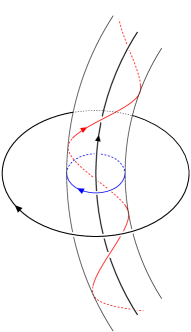
Figure 1.

The isotopy from $K_{1}$ to $K^{\prime}_{1}$ can be extended to an isotopy of tubular neighborhoods from $N_{1}$ to $N_{1}^{\prime}\subset V_{2}$, whose boundary is parallel to $\partial V_{2}$. Now $L$ is obtained by cutting $N_{1}^{\prime}$ out of $V_{2}$ and pasting $V_{1}$ in its place, with the identification between $\partial N^{\prime}_{1}$ and $\partial V_{1}$ given by a new gluing map $\varphi_{1}^{\prime}$. Notice that, since $V_{2}\setminus N^{\prime}_{1}$ is diffeomorphic to $T^{2}\times[0,1]$, we may unambiguously take $(\ell_{2},m_{2})$ as a basis for the domain of $\varphi^{\prime}_{1}$ (regarded as a map between homology groups). With this assumption, $\varphi^{\prime}_{1}$ is represented by the same matrix as $\varphi_{1}$. In fact, as already observed, $K^{\prime}_{1}$ and $\ell_{2}$ are isotopic as oriented knots, and $K^{\prime}_{1}$ admits $m_{2}$ as a right-hand-oriented meridian. Hence, $\ell_{2}$ and $m_{2}$ also play the role of the original $\lambda_{1}$ and $\mu_{1}$. Moreover, it makes sense to consider the composition

$$\varphi_{1}^{\prime}\circ\varphi_{2}\thinspace\colon H_{1}(\partial N_{2})\stackrel{{\scriptstyle\varphi_{2}}}{{\longrightarrow}}H_{1}(\partial V_{2})=H_{1}(N^{\prime}_{1})\stackrel{{\scriptstyle\varphi^{\prime}_{1}}}{{\longrightarrow}}H_{1}(\partial V_{1}),$$

which is represented by the matrix $A_{a_{1}}\cdot A_{a_{2}}$. This concludes the description of the $SL_{2}(\mathbb{Z})$-slam-dunk when $t=2$.

We now describe the construction for $t>2$ (assuming $n\geq 3$). We first apply an $SL_{2}(\mathbb{Z})$-slam-dunk to the first component, so that $K_{1}$ is removed from the chain link. Now $K_{2}$ is a meridian of $K_{3}$, so we can apply another $SL_{2}(\mathbb{Z})$-slam-dunk along $K_{2}$, and so on. In general, for each $1\leq i<t$ we remove a tubular neighborhood $N^{\prime}_{i}$ of the core of $V_{i+1}$, and identify its boundary with $\partial V_{i}$ via a gluing map $\varphi^{\prime}_{i}$ represented by $A_{a_{i}}$ with respect to the bases $(\ell_{i+1},m_{i+1})$ and $(\ell_{i},m_{i})$. By construction, for each $t=2,\ldots,n$ the composition of gluing maps

$$\varphi^{\prime}_{1}\circ\cdots\circ\varphi^{\prime}_{t-1}\circ\varphi_{t}\thinspace\colon H_{1}(\partial N_{t})\longrightarrow H_{1}(\partial V_{1})$$

identifies $\mu_{t}=-\varphi_{t}^{-1}(\ell_{t})$ with a curve whose coordinates with respect to $\ell_{1}$ and $m_{1}$ are given by the second column of $A_{a_{1}}\cdots A_{a_{t}}$. Similarly, after gluing, the coordinates of $\lambda_{t}$ with respect to $\ell_{1}$ and $m_{1}$ are given by the first column of $A_{a_{1}}\cdots A_{a_{t}}$. This proves (1) and (2).

To prove (3) we choose $t=n$, so that the modified link has a single component. The result of gluing together all the “layers” $V_{i+1}\setminus N^{\prime}_{i}$ for $i<n$ is diffeomorphic to $T^{2}\times[0,1]$ and the boundaries of the glued-up pieces are parallel tori. Moreover, the diffeomorphism with $T^{2}\times[0,1]$ can be chosen so that:

• $T^{2}\times\{0\}$ and $T^{2}\times\{1\}$ are identified with $\partial V_{1}$ and $\partial V_{n}$ respectively;

• the other parallel tori are identified with $T^{2}\times\{h\}$ for $n-2$ pairwise distinct values of $h\in(0,1)$.

This shows that $L(s)$ results from gluing two solid tori to $T^{2}\times[0,1]$. Moreover, the boundaries of the meridian disks of the solid tori are $m_{1}\subset T^{2}\times\{0\}$ and $\varphi_{n}(\lambda_{n})\subset T^{2}\times\{1\}$. By construction, the curve $\varphi_{n}(\lambda_{n})$ is isotopic to $p\ell_{1}+qm_{1}$, where

$$A_{a_{1}}\cdots A_{a_{n}}=\begin{pmatrix}p&a\\ q&b\end{pmatrix}\in SL_{2}(\mathbb{Z}).$$

Since $\left(\begin{smallmatrix}p&a\\ q&b\end{smallmatrix}\right)^{-1}=\left(\begin{smallmatrix}b&-a\\ -q&p\end{smallmatrix}\right)$, $L(s)$ is the result of a Dehn surgery with framing $\frac{p}{a}$ along an unknot, where $a(p-q)\equiv 1\bmod p$. Part (3) follows immediately from the fact that the lens spaces $L(p,q)$ and $L(p,q^{\prime})$ are orientation-preserving diffeomorphic when $qq^{\prime}\equiv 1\bmod p$. ∎

3. Proof of Theorem 1

The first part of Theorem 1 states that $B(s_{k,m})$ smoothly embeds in $\mathbb{CP}^{2}$ if $m$ is odd. We already observed in Section 1 that this is true if $k=-1$, therefore in the following we assume $k\geq 0$.

Consider the string $s_{k,m}$ of Section 1, with $k\geq 0$ and $m$ odd, and define:

• $s^{\prime}_{k,m}:=(2,(2^{[m-1]},m+2)^{[k+1]},1,2,(2^{[m-1]},m+2)^{[k+1]})$;

• $s^{\prime\prime}_{k,m}:=(2^{[m-1]},1,m+2,(2^{[m-1]},m+2)^{[k]},2^{[m]},1,m+2,(2^{[m-1]},m+2)^{[k]})$.

It is straightforward to check that the strings $s^{\prime}_{k,m}$ and $s^{\prime\prime}_{k,m}$ are both obtained from $s_{k,m}$ by changing some terms from $2$ to $1$, and that they both “blow-down” to $(0)$ in the sense of [7, Definition 2.1], therefore $L(s^{\prime}_{k,m})=L(s^{\prime\prime}_{k,m})=S^{1}\times S^{2}$.

Remark 2.

Applying [7, Lemma 2.4] to the string $s^{\prime}_{k,m}$ immediately implies that $L(s_{k,m})$ is of the form $L(p^{2},pq-1)$ for some $p>q\geq 1$.

Denote by $\nu_{2}\subset S^{1}\times S^{2}$ the curve corresponding to the meridian of the $\langle 1\rangle$-framed unknot of the diagram associated with $s^{\prime}_{k,m}$. In Section 2 the same meridian was denoted $\mu_{(k+1)m+2}$. Denote by $W$ the smooth 4-manifold with boundary obtained by viewing $S^{1}\times S^{2}$ as the boundary of $S^{1}\times D^{3}$ and attaching a 4-dimensional 2-handle along $\nu_{2}$ with framing $-1$. In view of [7, Theorem 1.1] and [8, Theorem 8.5.1], $W$ is orientation-preserving diffeomorphic to $B(s_{k,m})$.

We are going to prove Part (1) of Theorem 1 by showing that $\mathbb{CP}^{2}$ is obtained by attaching some 4-dimensional handles to $B(s_{k,m})$. First we attach two extra 2-handles along the meridians $\mu_{m}$ and $\mu_{(k+2)m+2}$, both with framing $1$. Notice that the indices $m$ and $(k+2)m+2$ give the positions where $s_{k,m}$ and $s^{\prime\prime}_{k,m}$ are different. As before, we rename these two meridians as $\nu_{3}$ and $\nu_{1}$ respectively, so that we encounter $\nu_{1}$, $\nu_{2}$ and $\nu_{3}$ in this order as we move along the diagram from right to left. Denote by $X$ the smooth $4$-manifold with boundary constructed so far. If we view $\nu_{1}$, $\nu_{2}$ and $\nu_{3}$ as part of a surgery presentation and blow them down we get a chain of unknots whose framing coefficients are exactly given by $s^{\prime\prime}_{k,m}$. This shows that the boundary of $X$ is $S^{1}\times S^{2}$. We can now add a $3-$handle and a $4-$handle to $X$ and obtain a closed $4-$manifold $\widehat{X}$.

Our plan is to show that $\widehat{X}$ is diffeomorphic to $\mathbb{CP}^{2}$. In order to do that, we view $\nu_{1},\nu_{2},\nu_{3}\subset S^{1}\times S^{2}$ as knots sitting inside a regular neighborhood $U$ of $\partial V_{1}\subset S^{1}\times S^{2}$ as in Part (1) of Proposition 2. The proof of Proposition 2 shows that $U$ can be identified with $T^{2}\times[0,1]$ in such a way that each $\nu_{i}$ is identified with a simple closed curve $T^{2}\times\{h_{i}\}$, where $1>h_{1}>h_{2}>h_{3}>0$. Moreover, the framing induced by $\partial N_{i}$ on $\nu_{i}$ coincides with the framing induced by $T^{2}\times\{h_{i}\}$. We introduce the notation

(3.1) $$(\nu_{1},\nu_{2},\nu_{3})=\left(\begin{pmatrix}p_{1}\\ q_{1}\end{pmatrix}_{\delta_{1}},\begin{pmatrix}p_{2}\\ q_{2}\end{pmatrix}_{\delta_{2}},\begin{pmatrix}p_{3}\\ q_{3}\end{pmatrix}_{\delta_{3}}\right)$$

to indicate that $\nu_{i}$ is $\delta_{i}$-framed (with $\delta_{i}=\pm 1$) with respect to the framing induced by $T^{2}\times\{h_{i}\}$ and the coordinates of the homology class of $\nu_{i}$ with respect to the basis $\ell_{1}$, $m_{1}$ are $(p_{i},q_{i})$.

If we view $S^{1}\times S^{2}$ as $L(s^{\prime}_{k,m})$, applying Part (2) of Proposition 2 for $t=n$ gives the standard presentation of $S^{1}\times S^{2}$ as $L((0))$, ie as $0$-surgery on an unknot. This way, $\partial V_{1}$ gets identified with the boundary of a neighborhood of such unknot, $m_{1}$ with a longitude and $\ell_{1}$ with a meridian.

Recall that, given a closed, oriented 3-manifold $M$ represented by a framed link with integer coefficients $\mathcal{L}$, there is a convenient way to represent handlebody decompositions of any $4$-dimensional cobordism $X$ obtained by attaching 4-dimensional handles to $M\times[0,1]$ along $M\times\{1\}$. In fact, the attaching curves of the 2-handles can always be isotoped into the complement of the glued-in solid tori of $M\times\{1\}$, so that each 2-handle can be represented as an additional framed knot in $S^{3}\setminus\mathcal{L}$. The union of all such framed knots with $\mathcal{L}$ is a relative Kirby diagram representing $X$. This representation requires a notation which distinguishes the role played by each component. If the framing coefficient of a knot $K$ is $n$, we are going to write it as $\langle n\rangle$ if $K$ is part of $\mathcal{L}$, and simply as $n$ if $K$ represents a 2-handle of $X$. Of course, we can also attach 3- and 4-handles as usual. There is a calculus for these handlebody presentations, usually called relative Kirby calculus. We refer the reader to [2, § 5.5] for further details.

We are going to apply relative Kirby calculus to the handle decomposition of $\widehat{X}$ we just described. It turns out that the effect of sliding the handle $h_{\nu_{i}}$ attached along $\nu_{i}$ over (an appropriate number of copies of) the handle $h_{\nu_{i+1}}$ attached over $\nu_{i+1}$, for $i=1,2$, was described in [11, Lemma 5.1]. In terms of our Notation (3.1), the action of such handle slides on the triples of coordinates is given by the following sliding map $F$, which can be applied to any two consecutive components of the triple as follows:

(3.2) $$F\left(\begin{pmatrix}p\\ q\end{pmatrix}_{\delta},\begin{pmatrix}p_{0}\\ q_{0}\end{pmatrix}_{\delta_{0}}\right)=\left(\begin{pmatrix}p_{0}\\ q_{0}\end{pmatrix}_{\delta_{0}},\begin{pmatrix}p-\delta_{0}\Delta_{0}p_{0}\\ q-\delta_{0}\Delta_{0}q_{0}\end{pmatrix}_{\delta}\right),\quad\text{where }\Delta_{0}=p_{0}q-q_{0}p.$$

Remark 3.

Recall that the curves $\nu_{i}$ are oriented, and therefore so are the handles $h_{\nu_{i}}$. The sliding map $F$ describes the change of coordinates of the homology classes of the attaching curves as a result of a handle addition of oriented 2-handles (cf. [2, §5.1]). On the other hand, the 4-manifold resulting from attaching a 2-handle does not depend on the choice of an orientation on the 2-handle, therefore a triple as in (3.1) can be modified by changing the signs of a pair $(p_{i},q_{i})$ (but not $\delta_{i}$) without changing the resulting 4-manifold up to diffeomorphisms.

Our strategy to prove that $\widehat{X}$ is diffeomorphic to $\mathbb{CP}^{2}$ will be as follows. We will exhibit a sequence of slides such that the coordinates $p_{i}$ and $q_{i}$ gradually get smaller, until we end up with a familiar Kirby diagram for $\mathbb{CP}^{2}$.

We now show that, for any pair $(k,m)$ as above, the map $F$ transforms the starting triple $(\nu_{1},\nu_{2},\nu_{3})$ into

$$\left(\begin{pmatrix}0\\ 1\end{pmatrix}_{1},\begin{pmatrix}1\\ 0\end{pmatrix}_{-1},\begin{pmatrix}1\\ 0\end{pmatrix}_{1}\right),$$

In order to do that we need to determine the coordinates $(p_{i},q_{i})$ of (3.1) in terms of $k$ and $m$. These will be given by products of $2\times 2$ matrices as in Proposition 2. Since the substring $(2^{[m-1]},m+2)$ occurs repeatedly in $s_{k,m}$, it will be useful to find a general formula for $A_{2}(A_{2}^{m-1}A_{m+2})^{l}$ (recall Notation 2.1). For this purpose, observe that an obvious induction gives

$$A_{2}^{m-1}=\begin{pmatrix}m&1-m\\ m-1&2-m\end{pmatrix}.$$

Then, define

$$C:=\begin{pmatrix}x+1&-1\\ x&-1\end{pmatrix}\in\text{GL}_{2}(\mathbb{Z}[x]).$$

It is easy to check that the matrix $A_{2}^{m-1}A_{m+2}$ is obtained by evaluating the entries of $C^{2}$ at $m$.

Now for $l\in\mathbb{Z}$ let $M_{l}:=A_{2}C^{l}$ and define the $\mathbb{Z}$-indexed sequences of polynomials $(P_{l})$, $(Q_{l})$, $(S_{l})$ and $(T_{l})$ by setting

(3.3) $$\begin{pmatrix}P_{l}&-S_{l}\\ Q_{l}&-T_{l}\end{pmatrix}:=M_{l}.$$

Since $C^{2}=xC+I$ we have $M_{l+2}=xM_{l+1}+M_{l}$, therefore each sequence satisfies the recursive formula

(3.4) $$f_{l+2}=x\cdot f_{l+1}+f_{l}.$$

Such sequences are completely determined by their values at two adjacent indices. Moreover,

• by setting $l=0$ in (3.3), we immediately get $P_{0}=2$, $Q_{0}=S_{0}=1$ and $T_{0}=0$;

• by setting $l=1$ and computing $A_{2}C$ we get $P_{1}=x+2$, $Q_{1}=x+1$ and $S_{1}=T_{1}=1$.

The following table shows a few terms of the four sequences:

$l$	$P_{l}$	$Q_{l}$	$S_{l}$	$T_{l}$
$-1$	$-x+2$	$1$	$1-x$	$1$
$0$	$2$	$1$	$1$	$0$
$1$	$x+2$	$x+1$	$1$	$1$
$2$	$x^{2}+2x+2$	$x^{2}+x+1$	$x+1$	$x$

The values in the table together with (3.4) imply that $S_{l}=Q_{l-1}$, therefore

$$M_{l}=A_{2}C^{l}=\begin{pmatrix}P_{l}&-Q_{l-1}\\ Q_{l}&-T_{l}\end{pmatrix}\quad\forall l\in\mathbb{Z}.$$

Lemma 4.

The sequences $(P_{l})$, $(Q_{l})$ and $(T_{l})$ satisfy the following identities:

$$(1)\hskip 5.0ptP_{l+1}-P_{l}=x\cdot Q_{l};\quad(2)\hskip 5.0ptQ_{l+1}-Q_{l}=x\cdot T_{l+1};\quad(3)\hskip 5.0ptQ_{l+1}+Q_{l}=P_{l+1};\quad(4)\hskip 5.0ptT_{l}+T_{l-1}=Q_{l};$$

$$(5)\hskip 5.0ptP_{l+1}Q_{l}-P_{l}Q_{l+1}=(-1)^{l+1}x;\quad(6)\hskip 5.0ptQ_{2l}Q_{2l-1}-P_{2l}T_{2l}=1;\quad(7)\hskip 5.0ptP_{2l}T_{2l-1}-Q_{2l-1}^{2}=1.$$

Proof.

Both sides of (1), (2), (3) and (4) are the terms of two sequences of polynomials satisfying the recursive formula (3.4), therefore it is enough to verify the identities for two distinct values of $l$, say $0$ and $1$. (5) We first claim that $(P_{l+1}Q_{l}-P_{l}Q_{l+1})$ is a geometric progression with common ratio $-1$: by (3.4), we have

$$P_{l+1}Q_{l}-P_{l}Q_{l+1}=(xP_{l}+P_{l-1})Q_{l}-P_{l}(xQ_{l}+Q_{l-1})=-(P_{l}Q_{l-1}-P_{l-1}Q_{l}),$$

which proves the claim. Now it is enough to verify the identity for $l=0$. (6) The LHS can be written as $\det(M_{2l})=\det(A_{2}C^{2l})$, which is immediately seen to be $1$, since $\det(A_{2})=\det(C^{2})=1$. Finally, (7) follows from (6) by substituting $Q_{2l}=P_{2l}-Q_{2l-1}$ and $T_{2l}=Q_{2l}-T_{2l-1}$, which is allowed by (3) and (4). ∎

We can now compute the coordinates $(p_{i},q_{i})$ of $\nu_{1}$, $\nu_{2}$ and $\nu_{3}$:

• $\nu_{3}$ is given by the first column of $A_{2}^{m-1}$, which is $\begin{pmatrix}m\\ m-1\end{pmatrix}$;

• $\nu_{2}$ is given by the first column of $A_{2}C^{2k+2}|_{x=m}=M_{2k+2}|_{x=m}$, which is $\begin{pmatrix}P_{2k+2}(m)\\ Q_{2k+2}(m)\end{pmatrix}$;

• $\nu_{1}$ is given by the first column of $A_{2}C^{2k+2}|_{x=m}A_{1}A_{2}^{m-1}=M_{2k+2}|_{x=m}A_{1}A_{2}^{m-1}$, which is

  $$M_{2k+2}|_{x=m}A_{1}\begin{pmatrix}m\\ m-1\end{pmatrix}=\begin{pmatrix}P_{2k+2}(m)&-Q_{2k+1}(m)\\ Q_{2k+2}(m)&-T_{2k+2}(m)\end{pmatrix}\begin{pmatrix}1\\ m\end{pmatrix}=\begin{pmatrix}P_{2k+1}(m)\\ Q_{2k+1}(m)\end{pmatrix},$$

  where the last equality holds by Identities (1) and (2) of Lemma 4.

Therefore, if for any pair $(l,m)$ of integers we define

$$\tau_{l,m}:=\left(\begin{pmatrix}P_{l+1}(m)\\ Q_{l+1}(m)\end{pmatrix}_{(-1)^{l}},\begin{pmatrix}P_{l+2}(m)\\ Q_{l+2}(m)\end{pmatrix}_{(-1)^{l+1}},\begin{pmatrix}m\\ m-1\end{pmatrix}_{1}\right),$$

the starting triple that arises from $B(s_{k,m})$ via the previous construction is $\tau_{2k,m}$.

Lemma 5.

The following hold:

• $\tau_{l,m}$ can be transformed into $\tau_{l+1,m}$ by applying the sliding map $F$ to the first two components;

• any pair of the form $\left(\begin{pmatrix}a+2\\ a+1\end{pmatrix}_{1},\begin{pmatrix}a\\ a-1\end{pmatrix}_{1}\right)$ can be transformed into $\left(\begin{pmatrix}a\\ a-1\end{pmatrix}_{1},\begin{pmatrix}a-2\\ a-3\end{pmatrix}_{1}\right)$ by applying $F$ and changing the signs in the second component;

• $F^{3}\left(\begin{pmatrix}0\\ 1\end{pmatrix}_{1},\begin{pmatrix}1\\ 0\end{pmatrix}_{-1}\right)=\left(\begin{pmatrix}2\\ 1\end{pmatrix}_{-1},\begin{pmatrix}3\\ 2\end{pmatrix}_{1}\right)$.

Proof.

We immediately see from (3.2) that $\tau_{l,m}$ is transformed into

$$\left(\begin{pmatrix}P_{l+2}(m)\\ Q_{l+2}(m)\end{pmatrix}_{(-1)^{l+1}},\begin{pmatrix}P_{l+1}(m)-\delta_{0}\Delta_{0}P_{l+2}(m)\\ Q_{l+1}(m)-\delta_{0}\Delta_{0}Q_{l+2}(m)\end{pmatrix}_{(-1)^{l}},\begin{pmatrix}m\\ m-1\end{pmatrix}_{1}\right),$$

which clearly agrees with $\tau_{l+1,m}$ at the first and the third components and at the framing of the second one. Therefore, we are left with verifying that

$$P_{l+1}(m)-\delta_{0}\Delta_{0}P_{l+2}(m)=P_{l+3}(m)\quad\text{and}\quad Q_{l+1}(m)-\delta_{0}\Delta_{0}Q_{l+2}(m)=Q_{l+3}(m).$$

By (3.4), both these equalities follow from $\delta_{0}\Delta_{0}=-m$: this is true because

$$\delta_{0}\Delta_{0}=(-1)^{l+1}(P_{l+2}(m)Q_{l+1}(m)-P_{l+1}(m)Q_{l+2}(m))=(-1)^{l+1}(-1)^{l}m=-m$$

where the second equality holds by Lemma 4(5). This proves (1). Finally, (2) and (3) follow from a straightforward computation; in particular, in order to prove (3), it is useful to observe that the quantity $\delta_{0}\Delta_{0}$ stays unchanged at each step, since both $\delta_{0}$ and $\Delta_{0}$ change sign. ∎

Now, in order to prove Theorem 1(1), we must show that the triple $\tau_{2k,m}$ corresponds to a Kirby diagram for $\mathbb{CP}^{2}$. By Lemma 5(1), it is enough to prove this for

$$\tau_{-1,m}=\left(\begin{pmatrix}2\\ 1\end{pmatrix}_{-1},\begin{pmatrix}m+2\\ m+1\end{pmatrix}_{1},\begin{pmatrix}m\\ m-1\end{pmatrix}_{1}\right).$$

We can apply Lemma 5(2) several times to the last two components. Observe that all coordinates decrease by $2$ at each step and recall that $m$ is odd. After $\frac{m-1}{2}$ applications of Lemma 5(2) we get

$$\left(\begin{pmatrix}2\\ 1\end{pmatrix}_{-1},\begin{pmatrix}3\\ 2\end{pmatrix}_{1},\begin{pmatrix}1\\ 0\end{pmatrix}_{1}\right),$$

and finally, applying Lemma 5(3) to the first two components,

$$\left(\begin{pmatrix}0\\ 1\end{pmatrix}_{1},\begin{pmatrix}1\\ 0\end{pmatrix}_{-1},\begin{pmatrix}1\\ 0\end{pmatrix}_{1}\right).$$

The last step in the proof of Theorem 1(1) is the following:

Lemma 6.

The triple $\left(\begin{pmatrix}0\\ 1\end{pmatrix}_{1},\begin{pmatrix}1\\ 0\end{pmatrix}_{-1},\begin{pmatrix}1\\ 0\end{pmatrix}_{1}\right)$ corresponds to a Kirby diagram for $\mathbb{CP}^{2}$.

Proof.

We have three knots in $T^{2}\times[0,1]\subset S^{1}\times S^{2}$, which can be glued to $V_{1}$ along $T^{2}\times\{0\}$ to form a new solid torus, which we regard as the exterior of an unknot $\widehat{K}$ in $S^{3}$ (as in the proof of Proposition 2). Consequently, we can regard $S^{1}\times S^{2}$ as the result of a Dehn surgery along $\widehat{K}$ with framing $0$. Now, the attaching curves $\nu_{1}$, $\nu_{2}$ and $\nu_{3}$ of the $2-$handles are contained in three nested tori, each of which bounds a regular neighborhood of $\widehat{K}$. More precisely, $\nu_{1}$ is a parallel copy of $m_{1}$, hence a canonical longitude of $\widehat{K}$, while $\nu_{2}$ and $\nu_{3}$ are two parallel copies of $\ell_{1}$, hence two unlinked meridians of both $\widehat{K}$ and $\nu_{1}$. The left-most picture of Figure 2 illustrates the resulting handlebody decomposition.

$\cup 3h\cup 4h$ at 60 -10 $\cup 3h\cup 4h$ at 220 10 $\cup 3h\cup 4h$ at 343 25 $\cup 4h$ at 422 25 $1$ at 20 82 $-1$ at 88 65 $1$ at 120 75 $1$ at 215 80 $0$ at 215 55 $1$ at 240 57 $0$ at 324 67 $1$ at 361 67 $1$ at 420 67

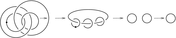
Figure 2.

Performing the handle slide indicated by the horizontal arrow yields the second picture of Figure 2, canceling the obvious $1$-$2$-handle pair yields the third picture, and canceling the $0$-framed unknot with the $3$-handle gives the well known Kirby diagram for $\mathbb{CP}^{2}$. ∎

By Lemmas 5 and 6, the 4-manifold $\widehat{X}$ is diffeomorphic to $\mathbb{CP}^{2}$. This proves the existence of the smooth embeddings, i.e. Part (1) of Theorem 1.

Part (2) of Theorem 1 follows from [9, Theorem 1] if $m=1$, so in the following we assume $m\geq 3$. By the results of Evans and Smith [1] recalled in Section 1, to show that $B(s_{k,m})$ does not symplectically embed in $\mathbb{CP}^{2}$ it suffices to write the lens space $L(s_{k,m})=\partial B(s_{k,m})$ as $L(p^{2},pq-1)$ and show that $p$ does not divide $q^{2}+9$. By Proposition 2 we can find such $p$ and $q$ by computing the first column of $M_{2k+2}A_{2}M_{2k+2}|_{x=m}$: we have

$$M_{2k+2}A_{2}M_{2k+2}\begin{pmatrix}1\\ 0\end{pmatrix}=\begin{pmatrix}P_{2k+2}&-Q_{2k+1}\\ Q_{2k+2}&-T_{2k+1}\end{pmatrix}\begin{pmatrix}2&-1\\ 1&0\end{pmatrix}\begin{pmatrix}P_{2k+2}\\ Q_{2k+2}\end{pmatrix}=$$

$$=\begin{pmatrix}P_{2k+2}&-Q_{2k+1}\\ Q_{2k+2}&-T_{2k+2}\end{pmatrix}\begin{pmatrix}2P_{2k+2}-Q_{2k+2}\\ P_{2k+2}\end{pmatrix}\stackrel{{\scriptstyle(3)}}{{=}}\begin{pmatrix}P_{2k+2}&-Q_{2k+1}\\ Q_{2k+2}&-T_{2k+2}\end{pmatrix}\begin{pmatrix}P_{2k+2}+Q_{2k+1}\\ P_{2k+2}\end{pmatrix}=$$

$$=\begin{pmatrix}P_{2k+2}^{2}\\ P_{2k+2}(Q_{2k+2}-T_{2k+2})+Q_{2k+1}Q_{2k+2}\end{pmatrix}\stackrel{{\scriptstyle(6)}}{{=}}\begin{pmatrix}P_{2k+2}^{2}\\ P_{2k+2}Q_{2k+2}+1\end{pmatrix}.$$

The numbers above the equality symbols denote which identities from Lemma 4 have been used. We can now obtain the first column of $M_{2k+2}A_{2}M_{2k+2}|_{x=m}$ by evaluating the above polynomials at $m$. We obtain $p=P_{2k+2}(m)$ and $q=P_{2k+2}(m)-Q_{2k+2}(m)\stackrel{{\scriptstyle(3)}}{{=}}Q_{2k+1}(m)$. By Lemma 4(7),

$$q^{2}+9=Q_{2k+1}(m)^{2}+9=P_{2k+2}(m)T_{2k+1}(m)+8,$$

which is a multiple of $P_{2k+2}(m)$ if and only if $P_{2k+2}(m)\ |\ 8$. However, we can easily observe that, for each $l\geq 1$, $P_{l}$ is a monic polynomial of degree $l$ with positive coefficients, so that $P_{2k+2}(m)\geq m^{2k+2}\geq m^{2}\geq 9$, and in particular $P_{2k+2}(m)\nmid 8$. This concludes the proof of Theorem 1.

References

[1]
J. Evans and I. Smith.
Markov numbers and Lagrangian cell complexes in the complex
projective plane.
Geometry & Topology, 22(2):1143–1180, 2018.
[2]
R. E. Gompf and A. I. Stipsicz.
4-manifolds and Kirby calculus.
Number 20 in Graduate Studies in Mathematics. American Mathematical
Soc., 1999.
[3]
P. Hacking and Y. Prokhorov.
Smoothable del Pezzo surfaces with quotient singularities.
Compositio Mathematica, 146(1):169–192, 2010.
[4]
T. Khodorovskiy.
Symplectic rational blow-up.
arXiv:1303.2581, 2013.
[5]
R. Kirby and P. Melvin.
Dedekind sums, -invariants and the signature cocycle.
Mathematische Annalen, 299(2):231–268, 1994.
[6]
J. Kollár.
Is there a topological Bogomolov-Miyaoka-Yau inequality?
Pure and Applied Mathematics Quarterly, 4(2):203–236, 2008.
[7]
P. Lisca.
On symplectic fillings of lens spaces.
Transactions of the American Mathematical Society,
360(2):765–799, 2008.
[8]
A. Némethi and P. Popescu-Pampu.
On the Milnor fibres of cyclic quotient singularities.
Proceedings of the London Mathematical Society,
101(2):554–588, 2010.
[9]
B. Owens.
Smooth, nonsymplectic embeddings of rational balls in the complex
projective plane.
The Quarterly Journal of Mathematics, 71(3):997–1007, 2020.
[10]
O. Riemenschneider.
Deformationen von Quotientensingularitäten (nach zyklischen
gruppen).
Mathematische Annalen, 209(3):211–248, 1974.
[11]
M. Tange and Y. Yamada.
Four-dimensional manifolds constructed by lens space surgeries along
torus knots.
Journal of Knot Theory and Its Ramifications, 21(11):1250111,
2012.