TRIX: Low-Skew Pulse Propagation for Fault-Tolerant Hardware

Abstract

The vast majority of hardware architectures use a carefully timed reference signal to clock their computational logic. However, standard distribution solutions are not fault-tolerant. In this work, we present a simple grid structure as a more reliable clock propagation method and study it by means of simulation experiments. Fault-tolerance is achieved by forwarding clock pulses on arrival of the second of three incoming signals from the previous layer.

A key question is how well neighboring grid nodes are synchronized, even without faults. Analyzing the clock skew under typical-case conditions is highly challenging. Because the forwarding mechanism involves taking the median, standard probabilistic tools fail, even when modeling link delays just by unbiased coin flips.

Our statistical approach provides substantial evidence that this system performs surprisingly well. Specifically, in an “infinitely wide” grid of height $H$, the delay at a pre-selected node exhibits a standard deviation of $O(H^{1/4})$ ($\approx 2.7$ link delay uncertainties for $H=2000$) and skew between adjacent nodes of $o(\log\log H)$ ($\approx 0.77$ link delay uncertainties for $H=2000$). We conclude that the proposed system is a very promising clock distribution method. This leads to the open problem of a stochastic explanation of the tight concentration of delays and skews. More generally, we believe that understanding our very simple abstraction of the system is of mathematical interest in its own right.

1 Introduction

When designing high reliability systems, any critical subsystem susceptible to failure must exhibit sufficient redundancy. Traditionally, clocking of synchronous systems is performed by clock trees or other structures that cannot sustain faulty components [23]. This imposes limits on scalability on the size of clock domains; for instance, in multi-processor systems typically no or only very loose synchronization is maintained between different processors [6, 18]. Arguably, this suggests that fault-tolerant clocking methods that are competitive – or even better – in terms of synchronization quality and other parameters (ease of layouting, amount of circuitry, energy consumption, etc.) would be instrumental in the design of larger synchronous systems.

To the best of our knowledge, at least until 20, or perhaps even 10 years ago, there is virtually no work on fault-tolerance of clocking schemes beyond production from the hardware community; due to the size and degree of miniaturization of systems at the time, clock trees and their derivatives were simply sufficiently reliable in practice. That this has changed is best illustrated by an upsurge of interest in single event upsets of the clocking subsystem in the last decade [1, 3, 4, 5, 14, 16, 20, 22]. However, with ever larger systems and smaller components in place, achieving acceptable trade-offs between reliability, synchronization quality, and energy consumption requires to go beyond these techniques.

On the other hand, there is a significant body of work on fault-tolerant synchronization from the area of distributed systems. Classics are the Srikanth-Toueg [19] and Lynch-Welch [21] algorithms, which maintain synchronization even in face of a large minority (strictly less than one third) of Byzantine faulty nodes. Going beyond this already very strong fault model, a line of works [7, 10, 11, 12, 15] additionally consider self-stabilization, the ability of a system to recover from an unbounded number of transient faults. The goal is for the system to stabilize, i.e., recover nominal operation, after transient faults have ceased. Note that the combination makes for a very challenging setting and results in extremely robust systems: even if some nodes remain faulty, the system will recover from transient faults, which is equivalent to recover synchronization when starting from an arbitrary state despite interference from Byzantine faulty nodes.

While these fault-tolerance properties are highly desirable, unsurprisingly they also come at a high price. All of the aforementioned works assume a fully connected system, i.e., direct connections between each pair of nodes. Due to the strong requirements, it is not hard to see that this is essentially necessary [9]: in order to ensure that each non-faulty node can synchronize to the majority of correct nodes, its degree must exceed the number of faults, or it might become effectively disconnected. In fact, it actually must have more correct neighbors than faulty ones, or a faulty majority of neighbors might falsely appear to provide the correct time. Note that emulating full connectivity using a crossbar or some other sparser network topology defeats the purpose, as the system then will be brought down by a much smaller number of faults in the communication infrastructure connecting the nodes. Accordingly, asking for such extreme robustness must result in solutions that do not scale well.

A suitable relaxation of requirements is proposed in [8]. Instead of assuming that Byzantine faults are also distributed across the system in a worst-case fashion, the authors of this work require that faults are “spread out.” More specifically, they propose a grid-like network they call HEX, through which a clock signal can be reliably distributed, so long as for each node at most one of its four in-neighbors is faulty. Note that for the purposes of this paper, we assume that the problem of fault-tolerant clock signal generation has already been sufficiently addressed (e.g. using [11]), but the signal still needs to be distributed. Provided that nodes fail independently, this means that the probability of failure of individual nodes that can likely be sustained becomes roughly $1/\sqrt{n}$, where $n$ is the total number of nodes; this is to be contrasted with a system without fault-tolerance, in which components must fail with probability at most roughly $1/n$. The authors also show how to make HEX self-stabilizing. Unfortunately, however, the approach has poor synchronization performance even in face of faults obeying the constraint of at most one fault in each in-neighborhood. While it is guaranteed that the clock signal propagates through the grid, nodes that fail to propagate the clock signal cause a “detour” resulting in a clock skew between neighbors of at least one maximum end-to-end communication delay $d$. This is much larger than the uncertainty $u$ in the end-to-end delay: As clocking systems can be (and are) engineered for this purpose, the end-to-end delay will vary between $d-u$ and $d$ for some $u\ll d$. To put this into perspective, in a typical system $u$ will be a fraction of a clock cycle, while $d$ may easily be half of a clock cycle or more.

This is inherent to the structure of the HEX grid, see Figure 1. It seeks to propagate the clock signal from layer to layer, where each node has two in-neighbors on the preceding and two in-neighbors on their own layer. Because the possibility of a fault requires nodes to wait for at least two neighbors indicating a clock pulse before doing so themselves, a faulty node refusing to send any signal implies that its two out-neighbors on the next layer need to wait for at least one signal from their own layer. This adds at least one hop to the path along which the signal is propagated, causing an additional delay of at least roughly $d$.

Our Contribution

Figure 1: A crashing node in a HEX grid causes a large skew between neighbors in the same layer, even with all links having exactly the same delay. Thick links cause nodes to pulse, dotted links mean that the transmitted pulse was too late to be considered, and faint dotted links do not transmit a pulse.

Figure 2: The basic topology of TRIX. Only wires incident to the central node are shown; the same pattern is applied at other nodes.

Figure 3: A crashing node in a TRIX grid causes no significant skew, compared to Figure 1. In fact, in absence of uncertainty, isolated crashes can be ignored entirely.

Figure 4: Worst-case assignment of wire delays causing large skew for TRIX. Squiggly lines indicate slow wires, straight ones fast wires. The symbol $\check{d}$ stands for $d-u$.

We propose a novel clock distribution topology that overcomes the above shortcoming of HEX. As in our topology nodes have in- and out-degrees of $3$ and it is inspired by HEX, we refer to it as TRIX; see Figure 2 for an illustration of the grid structure. Similar to HEX, the clock signal is propagated through layers, but for each node, all of its three in-neighbors are on the preceding layer. This avoids the pitfall of faulty nodes significantly slowing down the propagation of the signal. If at most one in-neighbor is faulty, each node still has two correct in-neighbors on the preceding layer, as demonstrated in Figure 3. Hence, we can now focus on fault-free executions, because single isolated faults only introduce an additional uncertainty of at most $u\ll d$. Predictions in this model are therefore still meaningful for systems with rare and non-malicious faults.

The TRIX topology is acyclic, which conveniently means that self-stabilization is trivial to achieve, as any incorrect state is “flushed out” from the system.

Despite its apparent attractiveness and even greater simplicity, we note that this choice of topology should not be obvious. The fact that nodes do not check in with their neighbors on the same layer implies that the worst-case clock skew between neighbors grows as $uH$, where $H$ is the number of layers and (for the sake of simplicity) we assume that the skew on the first layer (which can be seen as the “clock input”) is $0$, see Figure 4. However, reaching the skew of $d$ between neighbors on the same layer, which is necessary to give purpose to any link between them, takes many layers, at least $d/u\gg 1$ many. This is in contrast to HEX, where the worst-case skew is bounded, but more easily attained. When not assuming that delays are chosen in a worst-case manner, our statistical experiments show it to likely take much longer before this threshold is reached. Accordingly, in TRIX there is no need for links within the same layer for any practical number of layers, resulting in the advantage of smaller in- and out-degrees compared to HEX.

The main focus of this work lies on statistical experiments with the goal of estimating the performance of a TRIX grid as clock distribution method. Note that this is largely dominated by the skew between adjacent nodes in the grid, as these will drive circuitry that needs to communicate. While the worst-case behavior is easy to understand, it originates from a very unlikely configuration, where one side of the grid is entirely slow and the other is fast, see Figure 4. In contrast, correlated but gradual changes will also result in spreading out clock skews – and any change that affects an entire region in the same way will not affect local timing differences at all. This motivates to study the extreme case of independent noise on each link in the TRIX grid. Choosing a simple abstraction, we study the random process in which each link is assigned either delay $0$ or delay $1$ by an independent, unbiased coin flip. Moreover, we assume “perfect” input, i.e., each node on the initial layer signals a clock pulse at time $0$, and that the grid is infinitely wide. By induction over the layers, each node is then assigned the second largest value out of the three integers obtained by adding the respective link delay to the pulse time of each of its in-neighbors. We argue that this simplistic abstraction captures the essence of (independent) noise on the channels.

Due to the lack of applicable concentration bounds for such processes, we study this random process by extensive numerical experiments. Our results provide evidence that TRIX behaves surprisingly well in several regards, exhibiting better concentration than one might expect. First and foremost, the skew between neighbors appears to grow extremely slowly with the number of layers $H$. Even for $2000$ layers, we never observed larger differences than $7$ between neighbors on the same layer. Plotting the standard deviation of the respective distribution as a function of the layer, the experiments show a growth that is slower than doubly logarithmic, i.e. $\log\log H$. Second, for a fixed layer, the respective skew distribution exhibits an exponential tail falling as roughly $e^{-\lambda|x|}$ for $\lambda\approx 2.9$. Third, the distribution of pulsing times as a function of the layer (i.e., when a node pulses, not the difference to its neighbors) is also concentrated around its mean (which can easily be shown to be $H/2$), where the standard deviation grows roughly as $H^{1/4}$.

To support that these results are not simply artifacts of the simulation, i.e., that we sampled sufficiently often, we make use of the Dvoretzky-Kiefer-Wolfowitz (DKW) inequality [13] to show that the underlying ground truth is very close to the observed distributions. In addition, to obtain tighter error bounds for our asymptotic analysis of standard deviations as function of $H$, we leverage the Chernoff bound (as stated in [17]) on individual values. We reach a high confidence that the qualitative assertion that the TRIX distribution exhibits surprisingly good concentration is well-founded. We conclude that the simple mechanism underlying the proposed clock distribution mechanism results in a fundamentally different behavior than existing clock distribution methods or naive averaging schemes.

2 Preliminaries

Model

We model TRIX in an abstract way that is amenable to very efficient simulation in software. In this section, we introduce this model and discuss the assumptions and the resulting restrictions in detail.

The network topology is a grid of height $H$ and width $W$. For finite $W$, the left- and rightmost column would be connected, resulting in a cylinder. To simplify, we choose $W=\infty$, because we aim to focus on the behavior in large systems. Note that a finite width will work in our favor, as it adds additional constraints on how skews can evolve over layers; in the extreme case of $W=3$, in absence of faults skews could never become larger than $1$. We refer to the grid nodes by integer coordinates $(x,y)$, where $x\in\mathbb{Z}$ and $y\in\mathbb{N}_{0}$. Layer $0\leq\ell\leq H$ consists of the nodes $(x,\ell)$, $x\in\mathbb{Z}$.

Layer $0$ is special in that its nodes represent the clock source; they always pulse at time $0$. Again, there are implicit simplifications here. First, synchronizing the layer $0$ nodes requires a suitable solution – ideally also fault-tolerant – and cannot be done perfectly. However, our main goal here is to understand the properties of the clock distribution grid, so the initial skew is relevant only insofar as it affects the distribution. Some indicative simulations demonstrate that the grid can counteract “bad” inputs to some extent, but some configurations do not allow for this in a few layers, e.g. having all nodes with negative $x$ coordinates pulse much earlier than those with positive ones. Put simply, this would be a case of “garbage-in garbage-out,” which is not the focus of this study. A more subtle point is the unrealistic assumption that all layers of the grid have the same width. If the layer $0$ nodes are to be well-synchronized, they ought to be physically close; arranging them in a wide line is a poor choice. Accordingly, arranging the grid in concentric rings (or a similar structure) would be more natural. This would, however, entail that the number of grid nodes per layer should increase at a constant rate, in order to maintain a constant density of nodes (alongside constant link length, etc.). However, adding additional nodes permits to distribute skews better, therefore our simplification acts against us.

All other nodes $(x,\ell)$ for $\ell>0$ are TRIX nodes. Each TRIX node propagates the clock signal to the three nodes “above” it, i.e., the vertices $(x-1,y+1)$, $(x,y+1)$, and $(x+1,y+1)$. In the case of the clock generators, the signal is just the generated clock pulse; in case of the TRIX nodes, this signal is the forwarded clock pulse. Each node (locally) triggers the pulse, i.e., forwards the signal, when receiving the second signal from its predecessors; this way, a single faulty in-neighbor cannot cause the node’s pulse to happen earlier than the first correct in-neighbor’s signal arriving or later than the last such signal.

Pulse propagation over a comparatively long distance involves delays, and our model focuses on the uncertainty on the wires. Specifically, we model the wire delays using i.i.d. random variables that are fair coin flips, i.e., attain the values $0$ or $1$ with probability $1/2$ each. This reflects that any (known expected) absolute delay does not matter, as the number of wires is the same for any path from layer $0$ (the clock generation layer) to layer $\ell>0$; also, this normalizes the uncertainty to 1.

Formalizing the above, for each wire from the nodes $(x+c,y)$ with $c\in\{-1,0,+1\}$ to node $(x,y+1)$, we define $w_{c}$ to be the wire delay. We further define the time $t_{c}\mathrel{\vbox{\hbox{\scriptsize.}\hbox{\scriptsize.}}}=d(x+c,y)+w_{c}$ at which node $(x,y+1)$ receives the clock pulse. Then node $(x,y+1)$ fires a clock pulse at the median time $t\mathrel{\vbox{\hbox{\scriptsize.}\hbox{\scriptsize.}}}=\operatorname*{median}\{t_{-1},t_{0},t_{+1}\}$. As we assume that all clock generators (i.e., nodes with $y=0$) fire, by induction on $y$ all $d(x,y)$ are well-defined and finite.

This model may seem idealistic, especially our choice of the wire delay distribution. However, in Appendix 0.A we argue that this is not an issue.

We concentrate on two important metrics to analyze this system: absolute delay and relative skew. The total delay $d(x,y)$ of a node $(x,y)$ (usually with $y=H$) is the time at which this node fires. The relative skew $s^{\delta}(x,y)$ in horizontal distance $\delta$ is the difference in total delay; i.e., $s^{\delta}(x,y)\mathrel{\vbox{\hbox{\scriptsize.}\hbox{\scriptsize.}}}=d(x+h,y)-d(x,y)$. Our main interests are the random variables $d(H)\mathrel{\vbox{\hbox{\scriptsize.}\hbox{\scriptsize.}}}=d(0,H)$, i.e. the delay at the top, and $s(H)\mathrel{\vbox{\hbox{\scriptsize.}\hbox{\scriptsize.}}}=s^{1}(0,H)$, i.e. the relative skew between neighboring nodes.

Further Notation

We write $\mathcal{N}(\mu,\sigma^{2})$ to denote the normal distribution with mean $\mu$ and standard deviation $\sigma$.

Given the average sample value $\bar{v}=\sum_{i=1}^{n}v_{i}/n$ over a set of $n$ sample values $v_{i}$, we compute the empiric standard deviation as $(\sum_{i=1}^{n}(v_{i}-\bar{v})^{2}/(n-1))^{1/2}$.

We denote the cumulative distribution function of a random variable $X$ as $C[X]$; e.g. the term $C[X](x)$ denotes the probability that $X\leq x$. We denote the inverse function by $C^{-1}[X]$.

A quantile-quantile-plot relates two distributions $A$ and $B$. The simplest definition is to plot the domain of $A$ against the domain of $B$, using the function $C^{-1}[B](C[A](x))$.

We define the sample space $\Omega$ as the set of possible specific assignments of wire delays. If we need to refer to the value of some random variable $X$ in a sample $s\in\Omega$, we write $X[s]$.

3 Delay is Tightly Concentrated

3.1 Empiric Analysis

In this subsection, we examine $d(2000)$, which we formally defined in Section 2. Recall that $d(2000)$ is the delay at layer 2000. The results are similar for other layers and, as we will show in Section 3.3, do change slowly with increasing $H$.

For reference, consider a simpler system consisting of a sequence of nodes arranged in a line topology, where each node transmits a pulse once receiving the pulse from its predecessor. In this system, the delay at layer $H$ would follow a binomial distribution with mean $H/2=1000$ and standard deviation $\sqrt{H}/2=\sqrt{2000}/2\approx 22$. Recall that by the central limit theorem, for large $H$ this distribution will be very close to a normal distribution with the same mean and standard deviation. In particular, it will have an exponential tail.

Figure 5 shows the estimated probability mass function of $d(2000)$. The data was gathered using 25 million independent simulations; in Appendix 0.A we discuss how we ensured that the simulations are correct.

Observe that the shape looks like a normal distribution, as one might expect. However, it is concentrated much more tightly around its mean than for the simple line topology considered above: The empiric standard deviation of this sample is only 2.741.

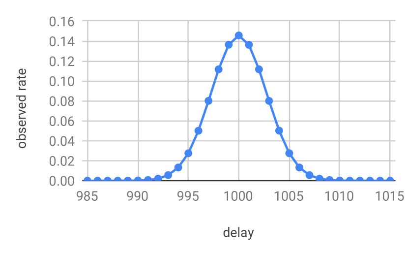
Figure 5: Estimated probability mass function of $d(2000)$.

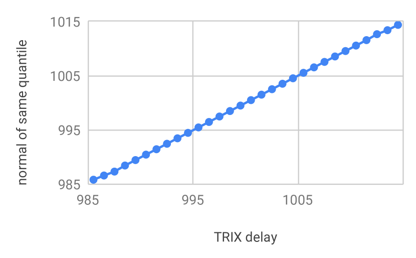
Figure 6: Quantile-quantile plot of $d(2000)$ against $N(1000,2.741^{2})$.

Figure 6 uses a quantile-quantile-plot to show that $d(2000)$ and $\mathcal{N}(1000,2.741^{2})$ seem to be close to identical, as indicated by the fact that the plot is close to a straight line. The extremes are an exception, where numerical and uncertainty issues occur. Of course, they cannot be truly identical, even if our guess $2.741$ was correct: $d(2000)$ is discrete and has a bounded support, in contrast to $\mathcal{N}(1000,2.741^{2})$. However, this indicates some kind of connection we would like to understand better.

The Dvoretzky-Kiefer-Wolfowitz inequality [13] implies that the true cumulative distribution function must be within $0.0003255$ (i.e., $8139$ evaluations) of our measurement with probability $1-\alpha=99\%$. For the values with low frequency however, the Dvoretzky-Kiefer-Wolfowitz inequality yields weak error bounds.

Instead, we use that Chernoff bounds can be applied to the random variable $X_{k}$ given by sum of variables $X_{i,k}$ indicating whether the $i$-th evaluation of the distribution attains value $k$. We then vary $p_{k}$, the unknown probability that the underlying distribution attains value $k$, and determine the threshold $p_{\max}$ at which Chernoff’s bound shows that $p_{k}\geq p_{\max}$ implied that our observed sample had an a-priori probability of at most $\alpha^{\prime}$; the same procedure is used to determine the threshold $p_{\min}$ for which $p_{k}\leq p_{\min}$ would imply that the observed sample has a-priori probability at most $\alpha^{\prime}$. Note that we can also group together multiple values of $k$ into a single bucket and apply this approach to the frequency of the overall bucket. This can be used to address all values with frequency $0$ together. Finally, we chose $\alpha^{\prime}$ suitably such that a union bound over all buckets yields the desired probability bound of $1-\alpha=99\%$ that all frequencies of the underlying distribution are within the computed error bounds.

Due to our large number of samples, the resulting error bars for the probability mass function are so small that they cannot be meaningfully represented in Figure 5; in fact, on the interval $[990,1010]$ the error bars are at most $8.05\%$ (multiplicative, not additive), and on the interval $[994,1006]$ at most $0.93\%$. On the other hand, data points outside $[990,1010]$ in Figure 6 should be taken as rough indication only.

In other words, we have run a sufficient number of simulations to conclude that the ground truth is likely to be very close to a binomial (i.e., essentially normal) distribution with mean $H/2=1000$ and standard deviation close to $2.741$; the former is easily shown, which we do next.

3.2 Stochastic Analysis

Lemma 1

$\mathbb{E}[d(H)]=H/2$.

Proof

Consider the bijection $f\colon\Omega\to\Omega$ on the sample space given by $f(s)=\bar{s}$, i.e., we exchange all delays of $0$ for delays of $1$ and vice versa. We will show that for a sample $s$ with $d(2000)[s]=\delta$ it holds that $d(2000)[f(s)]=H-\delta$. As the wire delays are u.i.d., all points in $\Omega$ have the same weight under the probability measure, implying that this is sufficient to show that $\mathbb{E}[d(H)]=H/2$.

We prove by induction on $y$ that $d(x,y)[f(s)]=y-d(x,y)[s]$ for all $0\leq y\leq H$ and $x\in\mathbb{Z}$; by the above discussion, evaluating this claim at $(x,y)=(0,H)$ completes the proof. For the base case of $y=0$, recall that $d(x,0)[f(s)]=d(x,0)[s]=0$ by definition.

For the step from $y$ to $y+1$, consider the node at $(x,y+1)$ for $x\in\mathbb{Z}$. For $c\in\{-1,0,+1\}$, the wire delay $w_{c}$ from $(x+c,y)$ to $(x,y+1)$ satisfies $w_{c}[f(s)]=1-w_{c}[s]$ by construction. By the induction hypothesis, $d(x+c,y)[f(s)]=y-d(x+c,y)[s]$. Together, this yields that $(x,y+1)$ receives the pulse from $(x+c,y)$ at time

$$d(x+c,y)[f(s)]+w_{c}[f(s)] =y+1-(d(x+c,y)[s]+w_{c}[s]).$$

We conclude that

$$d(x,y+1)[f(s)]=\,\operatorname*{median}_{c\in\{-1,0,1\}}\{y+1-(d(x+c,y)[s]+w_{c}[s])\}$$

$$=\,y+1-\operatorname*{median}_{c\in\{-1,0,1\}}\{d(x+c,y)[s]+w_{c}[s]\}=y+1-d(x,y+1)[s].$$

3.3 Asymptotics in Network Depth

As discussed earlier, forwarding the pulse signal using a line topology would result in $d(H)$ being a binomial distribution with mean $H/2$ and standard deviation $\sqrt{H}/2$. For $d(2000)$, we observe a standard deviation that is smaller by about an order of magnitude.

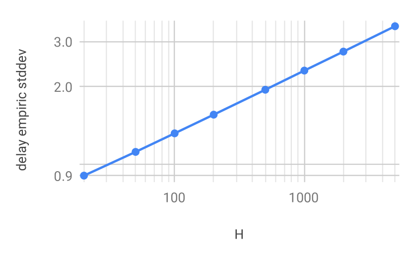
Figure 7: Log-log plot of the empiric standard deviation of $d(H)$ as a function of $H$.

Running simulations and computing the empiric standard deviation for various values of $H$ resulted in the data plotted in Figure 7 as a log-log plot. Using the technique discussed above, we can compute error bars. Again, the obtained error bounds cannot be meaningfully depicted; errors are about $1\%$ (multiplicative, not additive) with probability $1-\alpha=99\%$. The largest error margin is at 200 layers, with $1.35\%$.

Figure 7 suggests a polynomial relationship between standard deviation $\sigma$ and grid height $H$. The slope of the line is close to $1/4$, which suggests $\sigma\sim H^{\beta}$ with $\beta\approx 1/4$.

This is a quadratic improvement over the reference case of a line topology.

4 Skew is Tightly Concentrated

4.1 Empiric Analysis

In this subsection, we study $s(2000)$, which we formally defined in Section 2. Recall that $s(2000)$ is the skew at layer 2000 between neighboring nodes. As we will show in Section 4.3, the behavior for other layers is very similar. In particular, the skews increase stunningly slowly with $H$.

We gathered data from 20 million simulations, and see a high concentration around $0$ in Figure 9, with roughly half of the probability mass at $0$. Note that again the error bars cannot be represented meaningfully in Figure 9; in fact, on the interval $[-3,+3]$ the error bars are at most $6.1\%$ (multiplicative, not additive), and on the interval $[-2,+2]$ at most $1.4\%$.

Observe that the skew does not follow a normal distribution at all: The probability mass seems to drop off exponentially like $e^{-\lambda|x|}$ for $\lambda\approx 2.9$ (where $x$ is the skew), and not quadratic-exponentially like $e^{-x^{2}/(2\sigma^{2})}$, as it would happen in the normal distribution. The probability mass for $0$ is a notable exception, not matching this behavior.

The Dvoretzky-Kiefer-Wolfowitz inequality [13] implies that the true cumulative distribution function must be within $0.0005147$ (i.e., $5147$ evaluations) of our measurement with probability $1-\alpha=99\%$. In particular, observing skew $6$ twice without observing skew $-6$ is well within error tolerance.

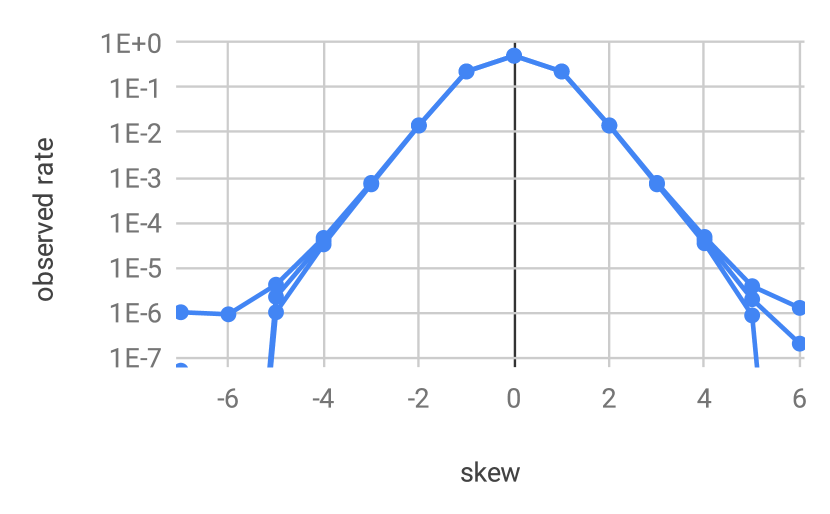
Figure 8: The estimated probability mass function for $s(2000)$, with a logarithmic y-axis. The error bounds are only visible at the fringes.

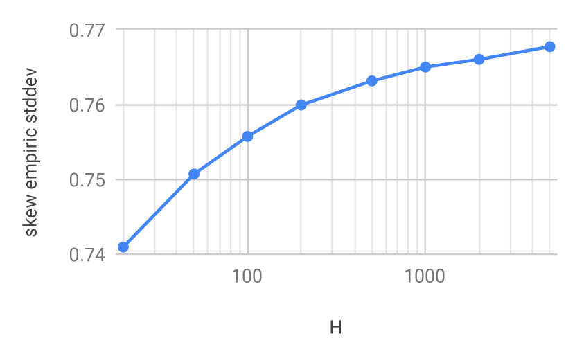
Figure 9: Empiric standard deviation of $s(H)$ as a function of $H$, as a log-lin plot.
 

4.2 Stochastic Analysis

First, we observe that the skew is symmetric with mean $0$. This is to be expected, as the model is symmetric. It also readily follows using the same argument as used in the proof of Lemma 1.

Corollary 1

$s(H)$ is symmetric with $\mathbb{E}[s(H)]=0$.

Proof

Consider the bijection used in the proof of Lemma 1. As shown in the proof, for any $(x,y)\in\mathbb{Z}\times\mathbb{N}_{0}$ and $s\in\Omega$, we have that

$$d(x,y)[f(s)]-d(x+1,y)[f(s)]=\, y-d(x,y)[s]-(y-d(x+1,y)[s])$$

$$=\, -(d(x,y)[s]-d(x+1,y)[s]).$$

Next we prove that the worst-case skew on layer $H$ is indeed $H$, c.f. Figure 4.

Lemma 2

There is a sample $s$ such that $s(H)[s]=H$.

Proof

In $s$, we simply let all wire delays $w_{i}$ of wires leading to a node with positive $x$ be $1$, and let all wire delays $w_{j}$ of wires leading into a node with non-positive $x$ be $0$. A simple proof by induction shows that for positive $x$ we get $d(x,y)[s_{1}]=y$ and for non-positive $x$ we get $d(x,y)[s_{1}]=0$. We conclude that $s(H)[s]=d(1,y)[s]-d(0,y)[s]=H$.

The constructed sample is not the only one which exhibits large skew. For example, simultaneously changing the delay of all wires between $x=0$ and $x=1$ does not affect times when nodes pulse. Moreover, for all $x\notin\{0,1\}$, we can concurrently change the delay of any one of their incoming wires without effect. It is not hard to see that the total probability mass of the described samples is small. We could not find a way to show that this is true in general; however, the experiments from Section 4.1 strongly suggests that this is the case. (Hence our question: How to approach statistical problems like this?)

4.3 Asymptotics in Network Depth

Again we lack proper models to describe the asymptotic behavior, and instead calculate the empiric standard deviation from sufficiently many simulations.

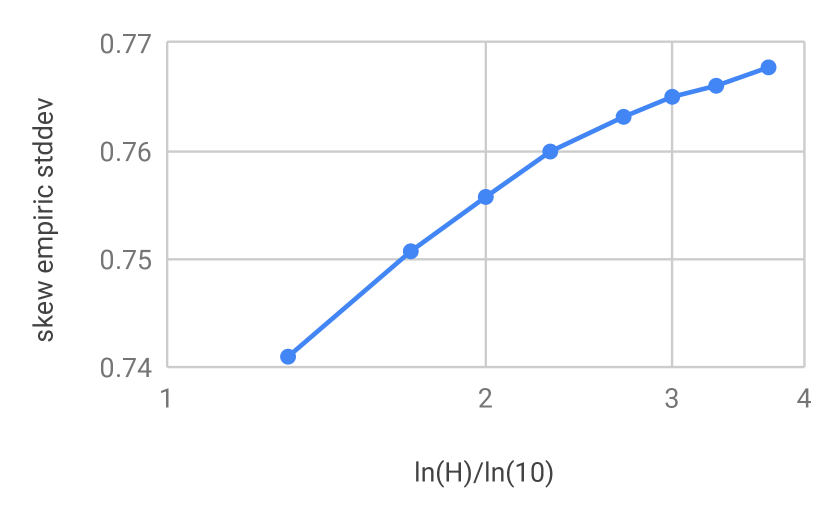
Figure 10: The data of fig. 9 in a loglog-lin plot.
 

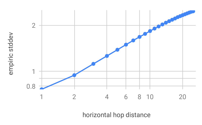
Figure 11: Empiric standard deviation of $s^{\delta}(0,500)$ as a function of horizontal distance $\delta$ in a log-log plot.

Figure 9 shows that the skew remains small even for large values of $H$. Note that the X-axis is logarithmic. Yet again, showing the error bars calculated using Chernoff bounds and DKW (Dvoretzky-Kiefer-Wolfowitz) is not helpful, as we get relative errors of about $0.6\%$ with $99\%$ confidence. The largest error margin is at 100 layers and below, with an error about $0.95\%$.

This suggests that the standard-deviation of $s(H)$ grows strongly sub-logarithmically, possibly even converges to a finite value. In fact, the data indicates a growth that is significantly slower than logarithmic: in Figure 11, the x-axis is doubly logarithmic. Thus, the plot suggests that $s(H)\in O(\log\log H)$.

Note that if we pretended that adjacent nodes exhibit independent delays, the skew would have the same concentration as the delay. In contrast, we see that adjacent nodes are tightly synchronized, implying strong correlation.

4.4 Asymptotics in Horizontal Distance

So far, we have limited our attention to the skew between neighboring nodes. In contrast, at horizontal distances $\delta\geq 2H$, node delays are independent, as they do not share any wires on any path to any clock generator. Therefore, the skew would be given by independently sampling twice from the delay distribution and taking the difference. It remains to consider how skews develop for smaller horizontal distances.

In Figure 11, we see that the skew grows steadily with increasing $\delta$. These simulations were run with $H=500$ for higher precision and execution speed. Note that the standard deviation of the skew converges to roughly $\sqrt{2}\cdot 1.95\approx 2.75$, i.e., $\sqrt{2}$ times the standard deviation of the delay at $H=500$, as $\delta$ approaches $2\cdot 500=1000$. This holds because the sum of independent random variables has variance equal to the sum of variances of the variables. As before, depicting the error bars determined by our approach is of no use, as relative errors are about $1.6\%$. The largest error margin is at horizontal distance 25, with $1.79\%$.

The small relative errors indicate that the log-log representation of the data is meaningful, and suggests that the standard deviation increases roughly proportional to $\delta^{\gamma}$ for $\gamma\approx 1/3$. It is not surprising that the slope falls off towards larger values, as we know that the curve must eventually flatten and become constant for $\delta\geq 2H=1000$. Overall, we observe that the correlation of skew at a distance is stronger than expected, specifically $\gamma\approx 1/3$ instead of the expected $\gamma\approx 1/2$ for small $\delta$.

5 Conclusion

In this work, we studied the behavior of the TRIX grid under u.i.d. link delays, using statistical tools. Our results clearly demonstrate that the TRIX grid performs much better than one would expect from naive solutions, and thus should be considered when selecting a fault-tolerant clock propagation mechanism.

Concretely, our simulation experiments show that the delay as function of the distance $H$ from the clock source layer is close to normally distributed with a standard deviation that grows only as roughly $H^{1/4}$, a qualitative change from e.g. a line topology that would not be achieved by averaging or similar techniques. Moreover, the skew between neighbors in the same layer is astonishingly small. While not normally distributed, there is strong evidence for an exponential tail, and the standard deviation of the distribution as function of $H$ appears to grow as $O(\log\log H)$. Checking the skew over larger horizontal counts $d$ (within the same layer) shows a less surprising pattern. However, still the increase as function of $d$ appears to be slightly slower than $\sqrt{d}$.

These properties render the TRIX grid an attractive candidate for fault-tolerant clock propagation, especially when compared to clock trees. We argue that our results motivate further investigation, considering correlated delays based on measurements from physical systems as well as simulation of frequency and/or non-white phase noise. In addition, the impact of faults, physical realization as less regular grid with a central clock source, and the imperfection of the input provided by the clock source need to be studied.

Last but not least, we would like to draw attention to the open problem of analyzing the stochastic process we use as an abstraction for TRIX. This is also the reason why we lack a purely mathematical analysis. While our simulation experiments are sufficient to demonstrate that the exhibited behavior is highly promising, gaining an understanding of the underlying cause would allow making qualitative and quantitative predictions beyond the considered setting. As both the nodes’ decision rule and the topology are extremely simple, one may hope for a general principle to emerge that can also be applied in different domains.

Appendix 0.A Potential Systematic Errors

In this section we discuss possible sources of systematic errors in our simulations and how we guarded against them.

0.A.1 Bugs

Since all experiments are software simulations, measurements have to be taken to insure against bugs. In this regard, there are several arguments to be made, some involving the Random Number Generator (RNG):

• We cross-validated four different implementations: (1) A very simple Python implementation that uses system randomness; (2) a slightly more involved Python implementation that exhaustively enumerates all possible wire delay combinations; (3) a straight-forward C implementation using system randomness; and (4) an optimized C implementation with the slightly weaker RNG “xoshiro512starstar” [2].

• Even though only implementation (4) was fast enough to be used to generate the bulk of the results, all implementations agree on the probability distributions of delay and skew for examples they can handle. Implementation (2) can only run up to layer 3 ($H\leq 3$), implementations (1) and (3) were used up to around layers 100 and 1000, respectively.

• Implementation (4) is short (200 lines, plus about 100 lines for the RNG [2]), and is simple enough to be inspected manually.

• Multiple machines were used, so hardware failure can be ruled out with sufficient confidence.

0.A.2 Randomness and Model

• Tests with a number of weak RNGs showed that TRIX seems to be robust against this kind of deviation.

• Explorative simulations and validation simulations were kept strictly separate.

• For most discussions we assumed $H=2000$, because this definitely covers all practical applications. In fact, we expect that many applications only need $H=200$ or even $H=20$. In this paper we use a large value for $H$ to show that the observed behavior is not a fluke that occurs due to low $H$, but that the growth of delay and skew as function of $H$ is indeed asymptotically slow.

• Using a larger domain only scales the result linearly, as expected.

• Using different wire delay models (e.g. choosing uniformly from $\{0,0.5,1\}$ instead of $\{0,1\}$) does not significantly change the result, and in fact improves it slightly, as expected.

• We only focused on fault-free executions. Observe that single isolated faults only introduce an additional uncertainty of at most 1 (recall the normalization $u=1$). As faults are (supposed to be) rare and not maliciously placed, this means that the predictions for fault-free systems have substantial and meaningful implications also for systems with faults.

Appendix 0.B Raw Data

In the following, we provide the data for all graphs.

Figure 5		Figure 6
x (delay)	y (rate)	x (delay)	y (normal)
985	0.00000012	985.5	985.843
986	0.00000040	986.5	986.615
987	0.00000140	987.5	987.338
988	0.00001076	988.5	988.457
989	0.00004740	989.5	989.460
990	0.00019060	990.5	990.462
991	0.00066280	991.5	991.457
992	0.00206788	992.5	992.464
993	0.00561240	993.5	993.470
994	0.01324480	994.5	994.472
995	0.02753772	995.5	995.475
996	0.05006436	996.5	996.479
997	0.08002964	997.5	997.486
998	0.11158960	998.5	998.492
999	0.13625144	999.5	999.498
1000	0.14553656	1000.5	1000.503
1001	0.13611860	1001.5	1001.508
1002	0.11158608	1002.5	1002.515
1003	0.07996644	1003.5	1003.520
1004	0.05016040	1004.5	1004.526
1005	0.02753824	1005.5	1005.531
1006	0.01324832	1006.5	1006.537
1007	0.00557100	1007.5	1007.542
1008	0.00205200	1008.5	1008.545
1009	0.00066300	1009.5	1009.545
1010	0.00018904	1010.5	1010.552
1011	0.00004660	1011.5	1011.556
1012	0.00001044	1012.5	1012.650
1013	0.00000144	1013.5	1013.385
1014	0.00000044	1014.5	1014.363
1015	0.00000008

Figure 11
hop dist.	empiric stddev
1	0.76334
2	0.94346
3	1.11873
4	1.26012
5	1.38309
6	1.49367
7	1.59118
8	1.67803
9	1.75621
10	1.83219
11	1.90233
12	1.96331
13	2.02323
14	2.07683
15	2.12580
16	2.17155
17	2.21355
18	2.25797
19	2.29356
20	2.32732
21	2.35812
22	2.38959
23	2.41912
24	2.44794
25	2.46569

	Figure 7	Figures 9 and 11
x ($H$)	y (stddev delay)	y (stddev skew)
20	0.9012352	0.74096549
50	1.1147817	0.75071102
100	1.3166986	0.75573837
200	1.5567596	0.75993333
500	1.9468302	0.76314438
1000	2.3115292	0.76499614
2000	2.7406959	0.76601516
5000	3.4405614	0.76771794

Figure 9
x (skew)	lowerb. rate	observed rate	upperb. rate
-7	0.0000000	0.0000001	0.0000010
-6	0.0000000	0.0000000	0.0000009
-5	0.0000010	0.0000022	0.0000041
-4	0.0000324	0.0000389	0.0000452
-3	0.0007020	0.0007322	0.0007578
-2	0.0142418	0.0143777	0.0144897
-1	0.2283952	0.2287592	0.2291231
0	0.5120736	0.5124375	0.5128015
1	0.2281477	0.2285116	0.2288756
2	0.0142291	0.0143650	0.0144769
3	0.0007024	0.0007326	0.0007583
4	0.0000343	0.0000410	0.0000475
5	0.0000009	0.0000020	0.0000038
6	0.0000000	0.0000002	0.0000013

References

- [1] Abouzeid, F., Clerc, S., Bottoni, C., Coeffic, B., Daveau, J.M., Croain, D., Gasiot, G., Soussan, D., Roche, P.: 28nm FD-SOI technology and design platform for sub-10pJ/cycle and SER-immune 32bits processors. In: ESSCIRC. pp. 108–111 (2015)
- [2] Blackman, D., Vigna, S.: Scrambled linear pseudorandom number generators. CoRR abs/1805.01407 (2018), http://arxiv.org/abs/1805.01407
- [3] Chipana, R., Kastensmidt, F.L.: SET Susceptibility Analysis of Clock Tree and Clock Mesh Topologies. In: ISVLSI. pp. 559–564 (2014)
- [4] Chipana, R., Kastensmidt, F.L., Tonfat, J., Reis, R.: SET susceptibility estimation of clock tree networks from layout extraction. In: LATW. pp. 1–6 (2012)
- [5] Chipana, R., Kastensmidt, F.L., Tonfat, J., Reis, R., Guthaus, M.: SET susceptibility analysis in buffered tree clock distribution networks. In: RADECS. pp. 256–261 (2011)
- [6] Culler, D., Singh, J.P., Gupta, A.: Parallel Computer Architecture: A Hardware/Software Approach. Morgan Kaufmann Publishers Inc. (1998)
- [7] Daliot, A., Dolev, D., Parnas, H.: Self-stabilizing Pulse Synchronization Inspired by Biological Pacemaker Networks. In: Proc. 6th International Symposium on Self-Stabilizing Systems (SSS). pp. 32–48 (2003)
- [8] Dolev, D., Függer, M., Lenzen, C., Perner, M., Schmid, U.: HEX: Scaling honeycombs is easier than scaling clock trees. J. Comput. Syst. Sci. 82(5), 929–956 (2016). https://doi.org/10.1016/j.jcss.2016.03.001
- [9] Dolev, D., Halpern, J.Y., Strong, H.R.: On the Possibility and Impossibility of Achieving Clock Synchronization. J. Comput. Syst. Sci. 32(2), 230–250 (1986)
- [10] Dolev, D., Hoch, E.N.: Byzantine Self-stabilizing Pulse in a Bounded-Delay Model. In: Proc. 9th International Symposium on Stabilization, Safety, and Security of Distributed Systems (2007). pp. 234–252 (2007)
- [11] Dolev, D., Függer, M., Lenzen, C., Schmid, U.: Fault-tolerant Algorithms for Tick-generation in Asynchronous Logic. J. ACM 61(5), 30:1–30:74 (2014)
- [12] Dolev, S., Welch, J.L.: Self-Stabilizing Clock Synchronization in the Presence of Byzantine Faults. Journal of the ACM 51(5), 780–799 (2004)
- [13] Dvoretzky, A., Kiefer, J., Wolfowitz, J.: Asymptotic minimax character of the sample distribution function and of the classical multinomial estimator. Ann. Math. Statist. 27(3), 642–669 (09 1956). https://doi.org/10.1214/aoms/1177728174
- [14] Gujja, A., Chellappa, S., Ramamurthy, C., Clark, L.T.: Redundant Skewed Clocking of Pulse-Clocked Latches for Low Power Soft Error Mitigation. In: RADECS. pp. 1–7 (2015)
- [15] Lenzen, C., Rybicki, J.: Self-Stabilising Byzantine Clock Synchronisation Is Almost as Easy as Consensus. J. ACM 66(5), 32:1–32:56 (2019). https://doi.org/10.1145/3339471
- [16] Malherbe, V., Gasiot, G., Clerc, S., Abouzeid, F., Autran, J.L., Roche, P.: Investigating the single-event-transient sensitivity of 65 nm clock trees with heavy ion irradiation and Monte-Carlo simulation. In: IRPS. pp. SE–3–1–SE–3–5 (2016)
- [17] Mitzenmacher, M., Upfal, E.: Probability and Computing: Randomized Algorithms and Probabilistic Analysis. Cambridge University Press (2005)
- [18] Patterson, D.A., Hennessy, J.L.: Computer Architecture: A Quantitative Approach. Morgan Kaufmann Publishers Inc. (1990)
- [19] Srikanth, T.K., Toueg, S.: Optimal Clock Synchronization. J. ACM 34(3), 626–645 (1987)
- [20] Wang, H.B., Mahatme, N., Chen, L., Newton, M., Li, Y.Q., Liu, R., Chen, M., Bhuva, B.L., Lilja, K., Wen, S.J., Wong, R., Fung, R., Baeg, S.: Single-Event Transient Sensitivity Evaluation of Clock Networks at 28-nm CMOS Technology. IEEE Trans. Nucl. Sci. 63(1), 385–391 (2016)
- [21] Welch, J.L., Lynch, N.A.: A New Fault-Tolerant Algorithm for Clock Synchronization. Information and Computation 77(1), 1–36 (1988)
- [22] Wissel, L., Heidel, D.F., Gordon, M.S., Rodbell, K.P., Stawiasz, K., Cannon, E.H.: Flip-Flop Upsets From Single-Event-Transients in 65 nm Clock Circuits. IEEE Trans. Nucl. Sci. 56(6), 3145–3151 (2009)
- [23] Xanthopoulos, T. (ed.): Clocking in Modern VLSI Systems. Springer (2009)