Event-shaped-dependent cumulants in p-Pb collisions at 5.02 TeV

Abstract

In this paper, we present a novel event-shaped cumulants (ESC) response approach, based on a multi-phase transport (AMPT) model simulations, to analyze p-Pb collisions at $\sqrt{s_{NN}}$= 5.02 TeV. We find that the Pearson coefficients between the subset cumulants of the final harmonics $v_{2}\{2k\}~{}(k=1,2,3,4)$ and the subset cumulants of initial eccentricity $\varepsilon_{2}\{2k\}$ in the ESC basis are significantly enhanced. These Pearson coefficients are strongly-dependent on the charged multiplicity, the set number of events (SNE), and only weakly-dependent on the order of the multi-particle cumulants (two-particles, four-particles, and so on). Our results show that the ESC method can suppress the event-by-event fluctuations.

Keywords: Event shaped cumulants; initial fluctuations; quark-gluon plasma;

I Introduction

One of the most remarkable achievements in ultra-relativistic heavy-ion experiments is the production of a fluidlike quark-gluon system, usually referred to as the quark-gluon plasma (QGP) Adams:2004pdo ; Song:2011acs . Collective harmonics flow plays a major role in probing the properties of QGP at the Relativistic Heavy Ion Collider (RHIC) of the Brookhaven National Laboratory (BNL) Abelev:2009lrr , and at the Large Hadron Collider (LHC) of the European Organization for Nuclear Research (CERN) ATLAS:2012mot . These collective flows may be well described by the hydrodynamic model Shen:2015saf ; Gale:2013eaf ; McDonald:2017hpf ; Calzetta:2020dtt ; Monnai:2021qeo , which show that the collective flow behavior is very sensitive to the energy density, and its fluctuations of the initial state.

To study the fluctuations of the initial state, Glauber, various hydrodynamic and transport models have been suggested, as well as approximate response relations between the final harmonics flow $v_{n}$ and the initial eccentricity $\varepsilon_{n}$ of large systems Enterria:2020pit ; Alver:2010tfi ; Noronha-Hostler:2015dbi ; Yan:2017ivm ; De:2018hri ; Bozek:2016tmc ; Floerchinger:2014soi ; Roch:2021foa . The hydrodynamic expectation is that $v_{n}/\varepsilon_{n}$ ratio increases monotonically with the transverse density across different collision energies and systems, and a violation of such a scaling may indicate an incorrect modeling of the initial transverse area and/or the azimuthal anisotropies $\varepsilon_{n}$ Enterria:2020pit .

Linear response relations for small systems, e.g., p-Pb and peripheral Pb-Pb collisions, have been also discussed in our previous work De:2020rli , and it has also been pointed out that a linear relation between the global $v_{2}\{2k\}~{}(k=1,2)$ and the global $\varepsilon_{2}\{2k\}$ in large hydrodynamic systems Qiu:2012hea , agrees with ALICE results (with the Kharzeev-Levin-Nardi initial conditions) Aamodt:2011hha . Furthermore, studies of multi-particle cumulants in the p-p Khachatryan:2016efc , p-Pb Khachatryan:2015efcm and p/d-Au Aidala:2018mom systems have revealed collective behavior similar to that found in heavier systems Chatrchyan:2013moh . The hydrodynamic Yan:2013ufe predictions for the multi-particle cumulants in p-Pb collisions, especially, the $v_{2}\{4\}/v_{2}\{2\}$ ratio is a fact that suggests a direct correlation of the final state harmonics with the initial state eccentricity.

The Pearson coefficient is a suitable quantity to describe such fluctuating response relation between the final harmonics flow $v_{n}$ and the initial eccentricity $\varepsilon_{n}$. Studies of nonzero Pearson coefficient in large systems have been presented  Niemi:2013edo ; Liu:2019pca , and also in high multiplicity p-Pb systems Yan:2014aad . However, the observed event-by-event Pearson coefficient is negligible in peripheral Pb-Pb collisions, which themselves include low multiplicity and may be referred to as a small system Rao:2019bpo .

In fact, it has been argued that if the system size is too small, and the lifetime is too short, a hydrodynamic approach with local isotropization Schenke:2017ooc may be not suitable. In addition, the presence of a collective flow in such a small systems is still being debated Dusling:2016ncp . Indeed, there are tremendous fluctuations in such small systems due to low multiplicity distribution, and a question naturally arises on whether a fluidlike QGP may be actually created  Nagle:2018ssc .

The nature of the fluctuating response between the final collective harmonics $v_{n}$ and the initial eccentricity $\varepsilon_{n}$ for small systems is still unclear both in hydrodynamic and transport models. On the other hand, the analysis of hydrodynamic models has revealed that even thought the system is small at the beginning, it may expand into a larger system in the final-states with large energy and entropy Heinz:2019hfi . Of course, one must be careful in assessing the flow fluctuations versus the nonflow ones in these small systems. One proposed solution to resolve the above questions about the smallest droplet of the QGP is to run polarized ion beams Bozek:2018efi , which is certainly an appealing suggestion but may take years to create the proper infrastructure to do so. To know what happened in such polarized ion collisions, one need to solve the dynamics with spin. The hydrodynamic model with spin has been calculated in the large systems Saha:2020fav ; Bhadury:2021ndi , while it still needs to be carefully verified in the small systems.

If we assume that a collective flow exists in these small reaction systems, then the analysis of fluctuations represents a very important tool to study the properties of the medium. To this aim, we here present a new type of event shaped cumulants (ESC) response approach for p-Pb collisions. This work follows our previous work, where we have discussed the response relations in p-Pb systems with event-by-event simulations De:2020rli . This work mainly discusses the event-by-event initial eccentricity fluctuations (except for the multiplicity fluctuations in Fig. 2), and does not intend to discuss the effects caused by other sources of fluctuations. In event-by-event small collisions, the fluctuations of the collective flow are mostly originating from the fluctuations of the initial geometry fluctuations and of the density. Therefore, we focus on the subset of events (SOE) cumulants response in p-Pb collisions using an ESC analysis. In the following, the ESC is proposed as an effective observation to suppress event-by-event initial geometry fluctuations.

The paper is organized as follows: In Sec. II we briefly describe the ESC response theory in a multi-phase transport (AMPT) model Lin:2004amt , which is then used in the simulations. The numerical results about the correlations between subsets of $v_{2}\{2k\}~{}(k=1,2,3,4)$ and subsets of $\varepsilon_{2}\{2k\}$ are presented in Sec. III. All of the produced charged pions in the calculations are chosen with 0.3 $<p_{T}<$ 3.0 GeV, $|\eta|<$1.0 and $80\leq M\leq 120$ (except for the multiplicity fluctuations in Fig. 2). Finally, we summarize our main results in Sec. IV.

II Materials and Methods

The AMPT model is a hybrid transport model for high-energy heavy ion collisions Lin:2004amt . The AMPT model can be produced particles in difference stages, from initial to final states. In AMPT model, the initial state particle distributions are generated by HIJING model Wang:1991hac . For this study, string melting is considered so that the produced hadrons from HIJING model are further converted into valence quarks and anti-quarks. Right before parton scatterings, we record the generated energy density profile of the system $\rho(\bm{x},\tau_{0})$, as the initial state of medium evolution. Initial state eccentricities of each event are then calculated with respect to Eq. (2). Parton scatterings, and accordingly the space-time evolution of QGP, are determined via ZPC parton cascade model Zhang:1998zac . After that, quarks and anti-quarks combine to form hadrons via a spatial coalescence model when scatterings stop. Hadronic phase of the system evolves according to a relativistic transport model until hadrons freeze-out. Note that it not only includes the medium matter but also includes the nonflow effects which are produced in hard scattering and hadron decay. To study the fluctuations of hydrodynamic property, we need a good physical quantity to describe the collective property of the medium, one is the fluctuating harmonic flow. To theoretically investigate these fluctuating behaviors, AMPT is an appropriate tool for the collective response analysis. More details about the AMPT model can be found in Ref. Lin:2004amt .

To study the event-by-event fluctuations, we start from the estimators of the harmonic flow $V_{n}$ and the initial eccentricity $E_{n}$, which have been studied in Ref. Alver:2010gr ,

$$V_{n}=v_{n}e^{in\Psi_{n}}\equiv\int\frac{d\phi}{2\pi}e^{in\phi_{p}}f(\phi_{p})\,,$$ (1)

and Ref. Teaney:2010vd ,

$$E_{n}=\varepsilon_{n}e^{in\Phi_{n}}\equiv-{\int d^{2}\bm{x}_{\perp}\rho(\bm{x}_{\perp},\tau_{0})r^{n}e^{in\phi}\over\int d^{2}\bm{x}_{\perp}r^{n}\rho(\bm{x}_{\perp},\tau_{0})}\,~{}~{}(n\geq 2).$$ (2)

where the magnitudes $v_{n}$ and $\varepsilon_{n}$ fluctuate on an event-by-event basis. The magnitudes $v_{n}$ and $\varepsilon_{n}$ in Eq. (1) and Eq. (2) can be accurately calculated by the event plane method Ma:2021pce , respectively. In this work, we focus on the second-order harmonic for the analyses. In turn, $V_{2}$ is found to be very sensitive to the event-by-event fluctuating initial eccentricity De:2018hri ; Nie:2019ioi , e.g., $v_{n}\{EP\}=\langle cos[n(\varphi-\Psi_{n})]\rangle$ and $\varepsilon_{n}=\sqrt{\langle r^{n}cos(n\phi)\rangle^{2}+\langle r^{n}sin(n\phi)\rangle^{2}}/\langle r^{n}\rangle$, where $\varphi$ is the azimuthal angle of the produced particle, and $\Psi_{n}$ is the corresponding symmetry event plane angle.

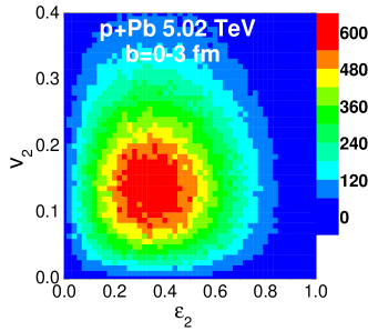
Figure 1: (Color online) Scatter plot of event-by-event $v_{2}$ from AMPT simulations for p-Pb (b=0-3 fm) collisions, as a function of $\varepsilon_{2}$.

Let us first explore the behavior of fluctuations in small systems using Eq. (1) and Eq. (2). Fig. 1 shows a scatter plot of event-by-event $v_{2}$ from AMPT simulations for p-Pb (b=0-3 fm) collisions, as a function of $\varepsilon_{2}$. One can see a plump distribution of points, which means that the event-by-event final harmonic flow is not correlated to the initial eccentricity, i.e. giant fluctuations and/or nonflow effects cannot be ignored in analyzing the phenomenon. The corresponding Pearson coefficient, evaluated as in Ref. De:2018hri is rather low $C(\varepsilon,v)\approx 0.04$. Similar results have been discussed in Ref. Rao:2019bpo , using a hydrodynamic model. Even though hydrodynamic arguments suggest that a cubic response should be considered, due to the initial fluctuations Rao:2019bpo , a complete understanding of the type of the response in such small system is still missing. In turn, such initial fluctuations may be described by the phase of $V_{2}$, such that the event plane may be the complex plane.

Another point to be taken account is the fact that the physics of p-A collisions may actually lie in the transition region between pure hydrodynamics and kinetic-particle evolution, as suggested by a kinetic theory analysis Kurkela:2019fia . The hydrodynamic model indeed fails to describe these kinetic-particle effects, which are referred to as nonflow effects. In turn, a weak Pearson coefficient implies that nonflow effects cannot be ignored in small systems. We conclude that the event-by-event Pearson coefficient may not represent the proper quantity to describe collective behaviors in such small systems, due to the finite multiplicity statistics.

To study the effective Pearson coefficient, an ESC method may be introduced. The multi-particle cumulants method is a useful tool in studying the global properties of correlations along the azimuthal direction in high-energy collisions Aaboud:2017mom .

Let us start with the calculation of $2k$-particle (where $k=1,2,3,4$) azimuthal correlations Borghini:2001nmf ; Bilandzic:2011faw ; Aaboud:2017mom

$$\langle 2\rangle \equiv \langle e^{i2(\phi_{1}-\phi_{2})}\rangle=\frac{|Q_{n}|^{2}-M}{M(M-1)},$$

$$\langle 4\rangle \equiv \langle e^{i2(\phi_{1}+\phi_{2}-\phi_{3}-\phi_{4})}\rangle=\frac{|Q_{n}|^{4}+|Q_{2n}|^{2}-2\cdot Re[Q_{2n}Q_{n}^{*}Q_{n}^{*}]-4(M-2)|Q_{n}|^{2}-2M(M-3)}{M(M-1)(M-2)(M-3)},$$

$$\langle 6\rangle \equiv \langle e^{i2(\phi_{1}+\phi_{2}+\phi_{3}-\phi_{4}-\phi_{5}-\phi_{6})}\rangle$$

$$= \{|Q_{n}|^{6}+9|Q_{2n}|^{2}|Q_{n}|^{2}-6\cdot Re[Q_{2n}Q_{n}Q_{n}^{*}Q_{n}^{*}Q_{n}^{*}]+4[Re[Q_{3n}Q_{n}^{*}Q_{n}^{*}Q_{n}^{*}]$$

$$- 3\cdot Re[Q_{3n}Q_{2n}^{*}Q_{n}^{*}]]+2[9(M-4)\cdot Re[Q_{2n}Q_{n}^{*}Q_{n}^{*}]+2|Q_{3n}|^{2}]-9[|Q_{n}|^{4}+|Q_{2n}|^{2}](M-4)$$

$$+ 18[|Q_{n}|^{2}(M-2)(M-5)]-6M(M-4)(M-5)\}$$

$$/ \{M(M-1)(M-2)(M-3)(M-4)(M-5)\},$$

$$\langle 8\rangle \equiv \langle e^{i2(\phi_{1}+\phi_{2}+\phi_{3}+\phi_{4}-\phi_{5}-\phi_{6}-\phi_{7}-\phi_{8})}\rangle$$ (3)

$$= \{|Q_{n}|^{8}-12\cdot Q_{2n}Q_{n}Q_{n}Q_{n}^{*}Q_{n}^{*}Q_{n}^{*}Q_{n}^{*}+6\cdot Q_{2n}Q_{2n}Q_{n}^{*}Q_{n}^{*}Q_{n}^{*}Q_{n}^{*}$$

$$+ 16\cdot Q_{3n}Q_{n}Q_{n}^{*}Q_{n}^{*}Q_{n}^{*}Q_{n}^{*}-96\cdot Q_{3n}Q_{n}Q_{2n}^{*}Q_{n}^{*}Q_{n}^{*}-12\cdot Q_{4n}Q_{n}^{*}Q_{n}^{*}Q_{n}^{*}Q_{n}^{*}$$

$$- 36\cdot Q_{2n}Q_{2n}Q_{2n}^{*}Q_{n}^{*}Q_{n}^{*}+96(M-6)\cdot Q_{2n}Q_{n}Q_{n}^{*}Q_{n}^{*}Q_{n}^{*}+72\cdot Q_{4n}Q_{2n}^{*}Q_{n}^{*}Q_{n}^{*}$$

$$+ 48\cdot Q_{3n}Q_{n}Q_{2n}^{*}Q_{2n}^{*}-64(M-6)\cdot Q_{3n}Q_{n}^{*}Q_{n}^{*}Q_{n}^{*}+192(M-6)\cdot Q_{3n}Q_{2n}^{*}Q_{n}^{*}-96\cdot Q_{4n}Q_{3n}^{*}Q_{n}^{*}$$

$$- 36\cdot Q_{4n}Q_{2n}^{*}Q_{2n}^{*}-144(M-7)(M-4)Q_{2n}Q_{n}^{*}Q_{n}^{*}+36|Q_{4n}|^{2}+64|Q_{3n}|^{2}|Q_{n}|^{2}$$

$$- 64(M-6)|Q_{3n}|^{2}+9|Q_{2n}|^{4}+36|Q_{n}|^{4}|Q_{2n}|^{2}-144(M-6)|Q_{2n}|^{2}|Q_{n}|^{2}$$

$$+ 72(M-7)(M-4)(|Q_{2n}|^{2}+|Q_{n}|^{4})-16(M-6)|Q_{n}|^{6}$$

$$- 96(M-7)(M-6)(M-2)|Q_{n}|^{2}+24M(M-7)(M-6)(M-5)\}$$

$$/ \{M(M-1)(M-2)(M-3)(M-4)(M-5)(M-6)(M-7)\}.$$

Here, $n$=2, and $\phi_{j}$ is the azimuthal angle of the $j$-th particle transverse momentum and pseudorapidity region in a single event, and the $Q$-vector is $Q_{n}=\sum_{j}^{M}e^{in\phi_{j}}$. $M$ is the number of particles. The single bracket indicates that all of present particles are averaged out in a single event. Using the calculated multi-particle azimuthal correlations, the second-order cumulants $c_{2}\{2k\}~{}(k=1,2,3,4)$ Borghini:2001nmf ; Bilandzic:2011faw ; Aaboud:2017mom are obtained after subtracting the correlations between $2k~{}(k\geq 1)$ particles and averaged in an SOE, i.e.,

$$c_{2}\{2\}(i) = \langle\langle 2\rangle\rangle_{i},$$

$$c_{2}\{4\}(i) = \langle\langle 4\rangle\rangle_{i}-2\cdot\langle\langle 2\rangle\rangle_{i}^{2},$$

$$c_{2}\{6\}(i) = \langle\langle 6\rangle\rangle_{i}-9\cdot\langle\langle 2\rangle\rangle_{i}\langle\langle 4\rangle\rangle_{i}+12\cdot\langle\langle 2\rangle\rangle_{i}^{3},$$

$$c_{2}\{8\}(i) = \langle\langle 8\rangle\rangle_{i}-16\cdot\langle\langle 6\rangle\rangle_{i}\langle\langle 2\rangle\rangle_{i}-18\cdot\langle\langle 4\rangle\rangle_{i}^{2}+144\cdot\langle\langle 4\rangle\rangle_{i}\langle\langle 2\rangle\rangle_{i}^{2}-144\cdot\langle\langle 2\rangle\rangle_{i}^{4}.$$ (4)

where $i$ is the $i$th SOE cumulant. The double brackets mean that the event-by-event correlations are averaged in the $i$th SOE cumulant.

In this work, we focus on the multi-particle cumulants in ESC analysis, rather than in total events. Calculations refer to a subset of total events and, as a result, the total calculations are divided in multiple ESC. In our simulations, we thus set the number of events (denoted by SNE) included in a SOE cumulant (eg. 20, 50, 200, 500 or more/less events per SOE cumulant). For a fixed number of total events, we have different numbers of SOE for different SNE parameters, e.g., if the total number of events is 5$\times 10^{5}$ and SOE is set to 25000, 10000, 2500 and 1000, then we have SNE=20, 50, 200 and 500, respectively. If the SOE cumulants $c_{2}\{2k\}(i)~{}(k=1,2,3,4)$ are free of nonflow correlations and only weakly affected by number fluctuations, they can be used to estimate the SOE harmonics $v_{2}$, which can be written as

$$v_{2}\{2\}(i) = \sqrt{c_{n}\{2\}(i)},$$

$$v_{2}\{4\}(i) = \sqrt[4]{-c_{n}\{4\}(i)},$$

$$v_{2}\{6\}(i) = \sqrt[6]{c_{n}\{6\}(i)/4},$$

$$v_{2}\{8\}(i) = \sqrt[8]{-c_{n}\{8\}(i)/33}.$$ (5)

Here, the collective flow is estimated using a cumulants expansion of multi-particle correlations, without determining the orientation of the event plane. The reason for this is that if the particles are correlated with the orientation of the event plane, then the information about the event plane orientation is erased. Note that the sample in the evaluation of SOE cumulants is not randomly selected. Events are sorted according to the eccentricity, from minimum to maximum, after the evolution of event-by-event, and then the event subsets are divided. Finally, the SOE cumulants harmonics flow $v_{2}\{2k\}(i)$ are used for the ESC analysis. The calculation of ESC for the initial eccentricity is similar to that of the ESC for final harmonics, however the initial partons are used.

In order to estimate the correlation between two different samples, the Pearson coefficient $C(A,B)$ is defined in ESC basis, as

$$C(A,B)=\frac{\sum_{i=1}^{N}[A(i)-\langle A\rangle][B(i)-\langle B\rangle]}{\sqrt{\sum_{i=1}^{N}[A(i)-\langle A\rangle]^{2}}\sqrt{\sum_{i=1}^{N}[B(i)-\langle B\rangle]^{2}}}.$$ (6)

where $i$ is the $i$-th sample of SOE and $\langle\ldots\rangle$ denotes the total SOE events averaged. $N$ is the total number of SOEs. The variables $A$ and $B$ could be samples such as the SOE cumulants of initial eccentricity or the SOE cumulants of final harmonics. Notice that the cumulants are real numbers, and thus the Pearson coefficient in Eq. (6) is a real number. In this case, $C(A,B)=1$ means that the two samples are linearly fully correlated, whereas and $C(A,B)=0$ corresponds to completely linearly uncorrelated quantities. In this work, we only study the degree of linear correlation of the samples, without entering the discussing about the possible nonlinear correlations, which are still under debate in small systems Rao:2019bpo ; De:2020rli .

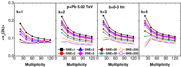
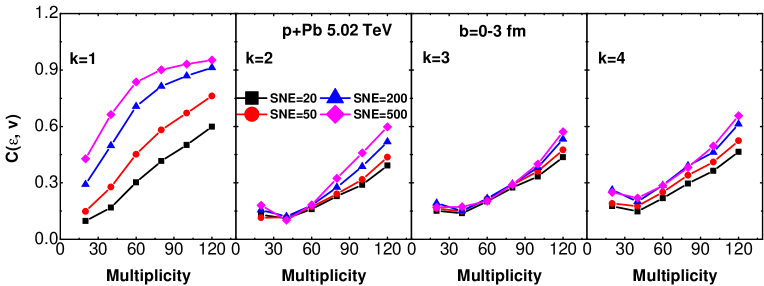
Figure 2: (Color online) Cumulants flow $\langle v_{2}\{2k\}\rangle$ and Pearson coefficients $C(\varepsilon,v)$ as functions of the charge multiplicity in p-Pb (b=0-3 fm, fixed number of events) collisions, respectively. Up panels: for the results of cumulants flow. Down panels: for the results of Pearson coefficients.

In this work, the Pearson coefficients between the SOE cumulants of the final harmonics and the SOE cumulants of the initial eccentricity are investigated for p-Pb (b=0-3 fm) collisions at $\sqrt{s_{NN}}$ = 5.02 TeV. We analyze the output charged pions using AMPT model Lin:2004amt . It takes the specific shear viscosity $\eta/s=0.273$, which is calculated by the Lund string fragmentation parameters in AMPT, i.e., $a=0.5$, $b=0.9$ GeV^-2, $\alpha_{s}$ =0.33 and $\mu$ = 3.2 fm^-1, which are suited for LHC De:2018hri ; De:2020rli . Here, we use different SNE parameters to simulate data and obtain the cumulants flow $\langle v_{2}\{2k\}\rangle$ and Pearson coefficients $C(\varepsilon,v)$ in p-Pb (b=0-3 fm) collisions. The impact parameters are controlled by the transverse distance of the overlap in the initial collisions space, and do not depend on the participant multiplicity $M$. As a consequence, our analysis includes a wide multiplicity range, from low $M$ to large ones, with a predominant range $M\leq 120$. The cumulants flow $\langle v_{2}\{2k\}\rangle$ are calculated from Eq. (II). And the Pearson coefficients $C(\varepsilon,v)$ between subset of $v_{2}$ and subset of $\varepsilon_{2}$ are calculated from Eq. (6). Both the cumulants flow $\langle v_{2}\{2k\}\rangle$ and Pearson coefficients $C(\varepsilon,v)$ dependent on the charged multiplicity, as shown in Fig. 2. They are strongly-dependent on the set number of events (SNE), and only weakly-dependent on the order of the multi-particle cumulants (two-particles, four-particles, and so on). The $\langle v_{2}\{2k\}\rangle$ decrease with the charged multiplicity (except for lower multiplicity $M<40$), while $C(\varepsilon,v)$ increase with the charged multiplicity. These results within smaller multiplicity are similar in Ref. Jia:2017rlm , due to the residual nonflow effects and/or fluctuations. Such newly developed subevent methods Jia:2017rlm is failed to suppress the residual nonflow contributions in small collisions. Note that the subevent method in Ref. Jia:2017rlm are ranged all sub-samples in a single event, while our results of sub-samples are acting at different events. In this work, we focus on suppressions of fluctuations with the subset of standard cumulants in the analysis. Therefore, for each chosen samples, its charged multiplicity is ranged in $M_{ch}\in[80,120]$. Such settings are used in Figs. 3, 4, 5 and 6. Note also that in this paper, we do not attempt to compare simulations with experimental data, but rather to explore how the correlations between the subset of final harmonic and subset of initial eccentricity are influenced by the initial fluctuations.

III Results

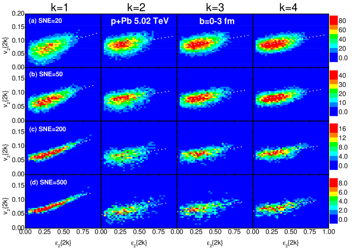
Figure 3: (Color online) Scatter plot of SOE cumulants $v_{2}\{2k\}~{}(k=1,2,3,4)$ from AMPT simulations for p-Pb (b=0-3 fm) collisions (at fixed number of events), as a function of SOE cumulants $\varepsilon_{2}\{2k\}$. The numbers $k=$1, 2, 3,  and 4 correspond to the two-particle, four-particle, six-particle and eight-particle cumulants, respectively. The number of SNE is set to 20, 50, 200, and 500, respectively.

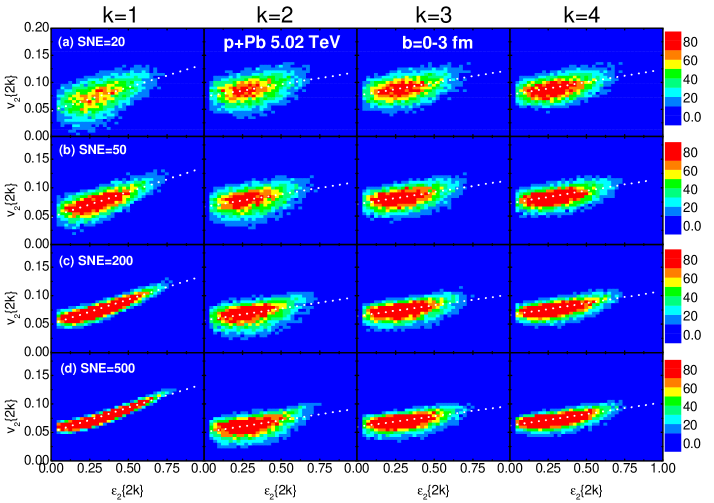
Figure 4: (Color online) As in Fig. 2, but for fixed scatter points (for different SNE, the number of scatter points is set by consistency).

The two-dimensional histograms in Figs. 3 and 4 show the correlation between the subset of $v_{2}\{2k\}~{}(k=1,2,3,4)$ and the subset of $\varepsilon_{2}\{2k\}$ for p-Pb (b=0-3 fm) collisions, respectively. To illustrate the nature of these correlations, we report the scatter plot for four different cases: (a) SNE=20; (b) SNE=50; (c) SNE=200 and (d) SNE=500.

Figure 3 shows the scatter plot of subset of $v_{2}\{2k\}~{}(k=1,2,3,4)$ from ESC AMPT simulations for p-Pb (b=0-3 fm) collisions, as a function of subset of $\varepsilon_{2}\{2k\}$. The numbers $k=$1, 2, 3, and 4 correspond to two-particle, four-particle, six-particle and eight-particle cumulants, respectively. The SNE is equal to 20, 50, 200 and 500 single events, respectively. Each point in Fig. 3 corresponds to a SOE cumulant. The white dashed line is the result of a linear least-square fitting. The value of the linear response coefficients is about 0.08. As it can be seen from Fig. 3, the $v_{2}\{2k\}~{}(k=2,3,4)$ coefficients are slightly correlated to the corresponding initial eccentricities $\varepsilon_{2}\{2k\}$ in all cases. In this work, we focus on the properties of fluctuations estimated by Pearson coefficient, but not on the response coefficients.

Figure 1 and 3 show that the SOE cumulants in Eq. (II) correspond to a thinner distribution of scattered points compared to the event-by-event method in Eq. (1) and Eq. (2). This means that the Pearson coefficient is larger (and correlations stonger) in the ESC basis rather than in event-by-event basis in this small systems. For SNE=500, we have $C(\varepsilon,v)\approx 0.560$ for four-particle, six-particle, and eight-particle cumulants, whereas $C(\varepsilon,v)\approx 0.07$ in event-by-event basis. We show the corresponding Pearson coefficient in Fig. 5. In that case $C(\varepsilon,v)\approx 0.560$, i.e., the harmonics are strongly dependent on the initial states. For larger SNE number, the shape of the scattered points cloud weakly depends on the order of multi-particle ($k>$1) cumulants. It has been pointed out that multi-particle cumulants method may suppress fluctuations Sirunyan:2019mcs . This is confirmed by our analysis, where ESC is also suppresses the fluctuations at different SNE parameters.

As a matter of fact, the cumulants framework may have limitations in describing $v_{n}$ fluctuations using a small set of cumulants Jia:2014efa due to the sizeable systematic uncertainties. As a consequence, we evaluate SOE cumulants to explore the effects of ESC fluctuations for a given impact parameter. As we mentioned above, fluctuations are suppressed in multi-particle cumulants. The Pearson coefficients of multi-particle cumulants ($k>$1) are smaller than the Pearson coefficient of two-particle cumulants ($k=$1). It should be also pointed out that in small systems response may be far from linear, and our results indicate that current linear response analysis may need to be carefully re-examined. We are planning to investigate this point elsewhere.

Looking at Fig. 3, one sees that correlations are weaker for low values of the SNE. In order to better investigate this point, we use a fixed number of scatter points for different SNE parameters, which are shown in Fig. 4. The total events are set as 5$\times 10^{5}$, 1.25$\times 10^{6}$, 5$\times 10^{6}$and 1.25$\times 10^{7}$, respectively, which corresponds to SNE=20, 50, 200 and 500, respectively. For these four different SNE parameters, the number of scatter points is set by consistency. Rather surprisingly, the distributions in Fig. 4 are similar to the distributions in Fig. 3. This means that the Pearson coefficients do not depend on the sample size (we show the Pearson coefficients in Fig. 5 (a) and (b)).

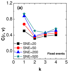
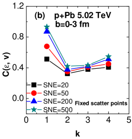
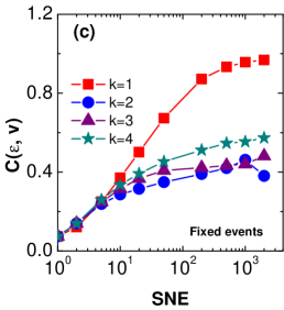
Figure 5: (Color online) Pearson coefficient as a function of the order of cumulants in p-Pb (b=0-3 fm) collisions. (a) Pearson coefficient at fixed number of events (from Fig. 3), (b) Pearson coefficient at fixed scatter points (from Fig. 4), and (c) SNE-dependent Pearson coefficient (at fixed number of events).

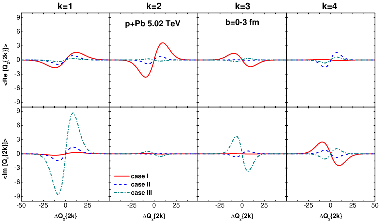
Figure 6: (Color online) Up panels: the averaged distribution of $Re~{}Q$ (real part of Q-vectors) as functions of Q-vectors difference $\triangle Q_{2}\{2k\}$ in p-Pb (b=0-3 fm) collisions at $\sqrt{s_{NN}}$= 5.02 TeV. Down panels: similar system with the up panels, but for the averaged distribution of $Im~{}Q$ (imaginary part of Q-vectors).

In order to evaluate the fluctuations of correlations, we use the Pearson coefficient $C(\varepsilon,v)$ and assess the linear correlation between the subset of $v_{2}\{2k\}~{}(k=1,2,3,4)$ and subset of $\varepsilon_{2}\{2k\}$. The Pearson coefficients $C(\varepsilon,v)$ are extracted from Fig. 3 and Fig. 4 using Eq. (6). Fig. 5 (a) and (b) shows the Pearson coefficients as functions of the order of multi-particle cumulants in p-Pb (b=0-3 fm) collisions, respectively. SNE are set to 20, 50, 200 and 500, respectively. Furthermore, Fig. 5 (c) shows the Pearson coefficients as a function of SNE in p-Pb (b=0-3 fm) collisions. The Pearson coefficients are significantly-dependent on the SNE number. They increase with increasing SNE, and achieve their maximum platform at SNE $\approx$ 1000, as shown in Fig. 5 (c). The Pearson coefficients are weakly-dependent on the order of multi-particle cumulants, except for the two-particle cumulants. As noted that these two-particle cumulants in the standard framework still retain the effects of unpredicted nonlinear response and fluctuations. Again, we focus on suppressions of fluctuations with the subset of standard cumulants method. Even if we increase the SNE, these Pearson coefficients are not normalized (with SNE$\geq$1000), because: (I) they include also the nonlinear dependence of the final harmonic on the initial eccentricity (see in Fig. 4), which has not been yet clarified Rao:2019bpo ; De:2020rli ; (II) the fluctuating final states include contributions not only from the initial fluctuations but also from the dynamical evolution stages Wei:2021pot . To fully quantify the fluctuations suppression effect caused by the multi-particle cumulants method, it may need more in-depth research and experimental data.

Here, to prove that the ESC method is not a simple result of events averaged in suppressing fluctuations, we show the results of Q-vector averaged distribution, $\langle Q_{2}\{2k\}\rangle$ ($k$=1, 2, 3, 4) in three different cases in Fig. 6. For Fig. 6, Case I: SNE=1 (noted as event-by-event simulations) for ESC; Case II: SNE=500 for the subset of cumulants, but without eccentricity re-sorted; Case III: SNE=500 for the subset of cumulants (this ESC method), but with eccentricity re-sorted. The results of up panels are the averaged distribution of Q-vectors (real part) in p-Pb (b=0-3 fm) collisions at $\sqrt{s_{NN}}$= 5.02 TeV and the results of down panels are the averaged distribution of Q-vectors (image part) in the same system. One can see that, the $\langle Q_{2}\{2k\}\rangle$ as functions of the $Q_{2}$ difference $\triangle Q_{2}\{2k\}=Q_{2}^{i}\{2k\}-\langle Q_{2}\{2k\}\rangle$ ($k$=1, 2, 3, 4, and $i$ is the $i$-th sample of SOE). The $\triangle Q_{2}\{2k\}$-dependent averaged distribution is inconsistent in these three cases, which shows that the ESC method is different from the conventional subset of cumulants (without concentration resorted) method in suppressing fluctuations.

IV Conclusions

In conclusion, we have put forward a novel approach to analyze p-Pb (b=0-3 fm) collisions at $\sqrt{s_{NN}}$= 5.02 TeV, based on ESC response and AMPT model simulations. We have found that the value of the Pearson coefficients between the subset cumulants of final harmonics $v_{2}\{2k\}~{}(k=1,2,3,4)$ and the subset cumulants of initial eccentricity $\varepsilon_{2}\{2k\}$ in the ESC basis is significantly enhanced. These Pearson coefficients are strongly-dependent on the SNE, and weakly-dependent on the order of multi-particle cumulants.

In our analysis, the use of ESC method leads to a suppression of the event-by-event fluctuations. Such suppression effects are more significant for larger SNE, e.g., the fluctuations for SNE$\geq$ 1000 are clearly more suppressed compared to the case SNE=1. In addition, by analyzing the cumulants for different SNE parameters, we have seen that the Pearson coefficients are clearly-dependent on the charged multiplicity.

Our results show that ESC analysis provides an enhancement of Pearson coefficients and, in turn, a mean for studying the fluctuations of fluidlike QGP in heavy-ion collisions.

References

- (1) J. Adams, C. Adler, M. M. Aggarwal, Z. Ahammed, J. Amonett, B. D. Anderson, M. Anderson, D. Arkhipkin, G. S. Averichev, S. K. Badyal, et al. [STAR Collaboration], Phys. Rev. Lett. 92, 052302 (2004) [arXiv:0306003 [nucl-ex]].
- (2) H. Song, S. A. Bass, U. Heinz, T. Hirano and C. Shen, Phys. Rev. Lett. 106, 192301 (2011) [arXiv:1011.2783 [nucl-th]].
- (3) B. Abelev, M. M. Aggarwal, Z. Ahammed, A. V. Alakhverdyants, B. D. Anderson, D. Arkhipkin, G. S. Averichev, J. Balewski, O. Barannikova, L. S. Barnby, et al. [STAR Collaboration], Phys. Rev. C 80, 064912 (2009) [arXiv:0909.0191 [nucl-ex]].
- (4) G. Aad, B. Abbott, J. Abdallah, S. Abdel Khalek, A. A. Abdelalim, A. Abdesselam, O. Abdinov, B. Abi, M. Abolins, O. S. AbouZeid, et al. [ATLAS Collaboration], Phys. Rev. C 86, 014907 (2012) [arXiv:1203.3087 [hep-ex]].
- (5) C. Shen, Z. Qiu, U. Heinz, Phys. Rev. C 92, 014901 (2015) [arXiv: 1502.04636[nucl-th]].
- (6) C. Gale, S. Jeon, B. Schenke, P. Tribedy, R. Venugopalan, Phys. Rev. Lett. 110, 012302 (2013) [arXiv: 1209.6330[nucl-th]].
- (7) S. McDonald, C. Shen, F. Fillion-Gourdeau, S. Jeon, C. Gale, Phys. Rev. C 95, 064913 (2017) [arXiv:1609.02958 [hep-ph]].
- (8) E. Calzetta, L. Cantarutti, Int. J. Mod. Phys. A 35, 2050074 (2020) [arXiv:1912.10562 [nucl-th]].
- (9) A. Monnai, B. Schenke, C. Shen, Int. J. Mod. Phys. A 36, 2130007 (2021) [arXiv:2101.11591 [nucl-th]].
- (10) D. d’Enterria, C. Loizides, Ann. Rev. Nucl. Part. Sci. 71, 315-344 (2020) [arXiv:2011.14909 [hep-ph]].
- (11) B. H. Alver, C. Gombeaud, M. Luzum, and J.-Y. Ollitrault, Phys. Rev. C 82, 034913 (2010) [arXiv:1007.5469 [nucl-th]].
- (12) J. Noronha-Hostler, L. Yan, F. G. Gardim and J.-Y. Ollitrault, Phys. Rev. C 93, 014909 (2016) [arXiv:1511.03896 [nucl-th]].
- (13) L. Yan, Chin. Phys. C 42, 042001 (2018) [arXiv:1712.04580 [nucl-th]].
- (14) D.-X. Wei, X.-G. Huang, L. Yan, Phys. Rev. C 98, 044908 (2018) [arXiv:1807.06299 [nucl-th]].
- (15) Piotr Bozek, Phys. Rev. C 93, 044908 (2016) [arXiv: 1601.04513[nucl-th]].
- (16) S. Floerchinger, U. A. Wiedemann, JHEP 08, 005 (2014) [arXiv: 1405.4393[hep-ph]].
- (17) H. Roch, N. Borghini, Eur. J. Phys. C 81, 380 (2021) [arXiv: 2012.02138[nucl-th]].
- (18) D.-X. Wei, L.-J. Zhou, X.-F. Li, Phys. Rev. C 102, 024917 (2020) [arXiv:1911.11011 [nucl-th]].
- (19) Z. Qiu, C. Shen, U. W. Heinz, Phys. Lett. B 707, 151 (2012) [arXiv:1011.3033 [nucl-th]].
- (20) K. Aamodt, B. Abelev, A. A. Quintana, D. Adamov, A. M. Adare, M. M. Aggarwal, G. A. Rinella, A. G. Agocs, A. Agostinelli, S. A. Salazar, et al. [ALICE Collaboration], Phys. Rev. Lett. 107, 032301 (2011) [arXiv:1105.3865 [nucl-ex]].
- (21) V. Khachatryan, A.M. Sirunyan, A. Tumasyan, W. Adam, E. Asilar, T. Bergauer, J. Brandstetter, E. Brondolin, M. Dragicevic, J. Er, et al. [CMS Collaboration], Phys. Lett. B 765, 193 (2017) [arXiv: 1606.06198[nucl-ex]].
- (22) V. Khachatryan, A.M. Sirunyan, A. Tumasyan, W. Adam, T. Bergauer, M. Dragicevic, J. Er, M. Friedl, R. Frhwirth, V.M. Ghete, et al. [CMS Collaboration], Phys. Rev. Lett. 115, 012301 (2015) [arXiv: 1502.05382[nucl-ex]].
- (23) C. Aidala, Y. Akiba, M. Alfred, V. Andrieux, K. Aoki, N. Apadula, H. Asano, C. Ayuso, B. Azmoun, V. Babintsev, et al. [PHENIX Collaboration], Phys. Rev. Lett. 120, 062302 (2018) [arXiv: 1707.06108[nucl-ex]].
- (24) S. Chatrchyan, V. Khachatryan, A.M. Sirunyan, A. Tumasyan, W. Adam, T. Bergauer, M. Dragicevic, J. Er, C. Fabjan, M. Friedl, et al. [CMS Collaboration], Phys. Rev. C 89, 044906 (2014) [arXiv: 1310.8651[nucl-ex]].
- (25) L. Yan, J.-Y. Ollitrault, Phys. Rev. Lett. 112, 082301 (2014) [arXiv: 1312.6555[nucl-th]].
- (26) H. Niemi, G.S. Denicol, H. Holopainen, P. Huovinen, Phys. Rev. C 87, 054902 (2013) [arXiv:1212.1008 [nucl-th]].
- (27) Z. Liu, W. Zhao, H. Song, Eur. Phys. J. C 79, 870 (2019) [arXiv:1903.09833 [nucl-th]].
- (28) L. Yan, J.-Y. Ollitrault, A. M. Poskanzer, Phys. Lett. B 742, 290 (2015) [arXiv:1408.0921 [nucl-th]].
- (29) S. Rao, M. Sievert and J. Noronha-Hostler, Phys. Rev. C 103, 034910 (2021) [arXiv:1910.03677 [nucl-th]].
- (30) B. Schenke, Nucl. Phys. A 967, 105 (2017) [arXiv:1704.03914 [nucl-th]].
- (31) K. Dusling, W. Li and B. Schenke, Int. J. Mod. Phys. E 25, 1630002 (2016) [arXiv:1509.07939 [nucl-ex]].
- (32) J. L. Nagle and W. A. Zajc, Ann. Rev. Nucl. Part. Sci. 68, 0211 (2018) [arXiv:1801.03477 [nucl-ex]].
- (33) U. W. Heinz and J. Scott Moreland, J. Phys. : Conf. Ser. 1271, 012018 (2019) [arXiv:1904.06592 [nucl-ex]].
- (34) P. Bozek, W. Broniowski, Phys. Rev. Lett. 121, 202301 (2018) [arXiv:1808.09840 [nucl-th]].
- (35) A. Saha, S. Sanyal, Int. J. Mod. Phys. E 29, 2050001 (2020) [arXiv:1902.08368 [hep-ph]].
- (36) S. Bhadury, J. Bhatt, A. Jaiswal, A. Kumar, Eur. Phys. J. ST 230, 655-672 (2021) [arXiv:2101.11964 [hep-ph]].
- (37) Z.-W. Lin, C. M. Ko, B.-A. Li, B. Zhang, S. Pal, Phys. Rev. C 72, 064901 (2005) [arXiv:nucl-th/0411110].
- (38) X.-N. Wang, M. Gyulassy, Phys. Rev. D 44, 3501 (1991).
- (39) B. Zhang, Comp. Phys. Comm. 109, 193 (1998) [arXiv:nucl-th/9709009].
- (40) B. Alver, G. Roland, Phys. Rev. C 81, 054905 (2010) [Erratum: Phys. Rev.C82,039903(2010)], [arXiv:1003.0194 [nucl-th]].
- (41) D. Teaney, L. Yan, Phys. Rev. C 83, 064904 (2011) [arXiv:1010.1876 [nucl-th]].
- (42) L. Ma, G.-L. Ma, Y.-G. Ma, Phys. Rev. C 103, 014918 (2021) [arXiv: 2102.01872 [nucl-th]].
- (43) M. Nie, L. Yi, X. Luo, G. Ma, J. Jia, Phys. Rev. C 100, 064905 (2019) [arXiv:1906.01422 [nucl-th]].
- (44) A. Kurkela, U. A. Wiedemann, B. Wu, Eur. Phys. J. C 79, 965 (2019) [arXiv: 1905.05139[hep-ph]].
- (45) M. Aaboud, G. Aad, B. Abbott, J. Abdallah, O. Abdinov, B. Abeloos, S.H. Abidi, O.S. AbouZeid, N.L. Abraham, H. Abramowicz, et al. [ATLAS Collaboration], Eur. Phys. J. C 77, 428 (2017) [arXiv:1705.04176 [hep-ex]].
- (46) N. Borghini, P. M. Dinh, J. Y. Ollitrault, Phys. Rev. C 63, 054906 (2001) [arXiv:0007063 [nucl-th]].
- (47) A. Bilandzic, R. Snellings, S. Voloshin, Phys. Rev. C 83, 044913 (2011) [arXiv:1010.0233 [nucl-ex]].
- (48) J. Jia, M. Zhou, A. Trzupek, Phys. Rev. C 96, 034906 (2017) [arXiv: 1701.03830[nucl-th]].
- (49) A.M. Sirunyan, A. Tumasyan, W. Adam, F. Ambrogi, E. Asilar, T. Bergauer, J. Brandstetter, M. Dragicevic, J. Er, A. Escalante Del Valle, et al. [CMS Collaboration], Phys. Rev. C 101, 014912 (2020) [arXiv: 1904.11519[nucl-ex]].
- (50) J. Jia, J. Phys. G 41, 024003 (2014) [arXiv: 1407.6057[nucl-ex]].
- (51) D.-X. Wei, Int. J. Mod. Phys. E 30, 2150084 (2021) [arXiv: 2107.03546 [nucl-th]].