A postprocessing technique for a discontinuous Galerkin discretization of time-dependent Maxwell’s equations

Abstract.

We present a novel postprocessing technique for a discontinuous Galerkin (DG) discretization of time-dependent Maxwell’s equations that we couple with an explicit Runge-Kutta time-marching scheme. The postprocessed electromagnetic field converges one order faster than the unprocessed solution in the $H(\operatorname{curl})$-norm. The proposed approach is local, in the sense that the enhanced solution is computed independently in each cell of the computational mesh, and at each time step of interest. As a result, it is inexpensive to compute, especially if the region of interest is localized, either in time or space. The key ideas behind this postprocessing technique stem from hybridizable discontinuous Galerkin (HDG) methods, which are equivalent to the analyzed DG scheme for specific choices of penalization parameters. We present several numerical experiments that highlight the superconvergence properties of the postprocessed electromagnetic field approximation.

Key words. time-domain electromagnetics, Maxwell’s equations, discontinuous Galerkin method, high-order method, postprocessing.

1. Introduction

Maxwell’s equations are the most general model of electrodynamic theory [14]. As a result, they are employed in a variety of applications, ranging from telecommunication engineering [17] to nanophotonics [12], to study the propagation of an electromagnetic field and its interaction with structures and matter.

Nowadays, numerical schemes are routinely employed to simulate the propagation of electromagnetic waves by computing approximate solutions to Maxwell’s equations [7]. While several approaches, such as finite difference methods [20], are available, we focus here on discontinuous Galerkin methods [11, 16, 19], which have recently received a lot of attention, due to their great flexibility and ability to handle complex geometries.

Even if currently available computational power allows for useful and realistic simulations, modeling accurately the propagation of electromagnetic fields in complex geometries is still a challenging and very costly task. As a result, numerical schemes are expected to be accurate and robust, but also very efficient and adapted to modern computer architectures.

In the context of finite element methods, postprocessing techniques are an attractive way to improve the accuracy of an already computed discrete approximation. In many cases, these techniques can increase the order of convergence of the method at a very moderate cost. In addition, they often have a “local” nature, which allows for the design of embarrassingly parallel implementations. As a result, postprocessing techniques and superconvergence have attracted a considerable attention in the past decades [2, 5, 6, 13].

In this work, we elaborate a novel postprocessing technique for time-dependent Maxwell’s equations. Following [19], Maxwell’s equations are discretized with a first-order discontinuous Galerkin method coupled with an explicit Runge-Kutta time-integration scheme [8]. This postprocessing improves the convergence rate in the $H(\operatorname{curl})$-norm by one order. As with similar postprocessing techniques devised in the past, our proposed approach is local, in the sense that the enhanced solution is computed independently in each cell of the computational mesh, and at each time step of interest. This is a key property as (a) it enables the design of highly parallel numerical algorithms, and (b) when the targeted application only requires the knowledge of the electromagnetic field in a limited region of space and/or time, the amount of computations is greatly reduced. Our postprocessing technique is inspired by two recent works, namely, a postprocessing for an explicit HDG discretization of the 2D acoustic wave equation [18], and a postprocessing for a HDG discretization of the 3D time-harmonic Maxwell’s equations [1].

We do not carry out the mathematical analysis of the proposed postprocessing but instead, we present a number of numerical experiments highlighting its main features. As a result, our work is organized as follows: in Section 2, we recall the settings and key notations related to Maxwell’s equations, discontinuous Galerkin methods, and Runge-Kutta schemes. We describe our postprocessing in Section 3, and Section 4 presents numerical illustrations of the resulting methodology.

2. Settings

2.1. Maxwell’s equations

We consider Maxwell’s equations set in a Lipschitz polyhedral domain $\Omega\subset\mathbb{R}^{3}$ and in a time interval $(0,T)$. Specifically, given $\boldsymbol{J}:(0,T)\times\Omega\to\mathbb{R}^{3}$, the electromagnetic field $\boldsymbol{E},\boldsymbol{H}:(0,T)\times\Omega\to\mathbb{R}^{3}$ satisfies

(1a) $$\left\{\begin{array}[]{rcl}\varepsilon\partial_{t}\boldsymbol{E}-\boldsymbol{\nabla}\times\boldsymbol{H}&=&\boldsymbol{J},\\ \mu\partial_{t}\boldsymbol{H}+\boldsymbol{\nabla}\times\boldsymbol{E}&=&\boldsymbol{0},\end{array}\right.$$

in $(0,T)\times\Omega$, where the functions $\varepsilon,\mu:\Omega\to\mathbb{R}$ respectively represent the electric permittivity and the magnetic permeability of the materials contained in $\Omega$. We assume that $0<c\leq\varepsilon,\mu\leq C$ a.e. in $\Omega$ for fixed constants $c$ and $C$.

The boundary of $\Omega$ is split into two subdomains $\Gamma_{\rm A}$ and $\Gamma_{\rm P}$, and we prescribe the boundary conditions

(1b) $$\left\{\begin{array}[]{rcll}\boldsymbol{E}\times\boldsymbol{n}_{\Omega}+\sqrt{\dfrac{\mu}{\varepsilon}}(\boldsymbol{H}\times\boldsymbol{n}_{\Omega})\times\boldsymbol{n}_{\Omega}&=&\boldsymbol{G}&\text{ on }(0,T)\times\Gamma_{\rm A},\\ \boldsymbol{E}\times\boldsymbol{n}_{\Omega}&=&\boldsymbol{0}&\text{ on }(0,T)\times\Gamma_{\rm P},\end{array}\right.$$

where $\boldsymbol{n}_{\Omega}$ denotes the unit vector normal to $\partial\Omega$ pointing outward $\Omega$ and $\boldsymbol{G}:(0,T)\times\Gamma_{\rm A}\to\mathbb{R}^{3}$ is a tangential load term (i.e. $\boldsymbol{G}\cdot\boldsymbol{n}_{\Omega}=0$). The first relation of (1b) is a first-order absorbing boundary condition (ABC) known as the Silver-Muller ABC. It is the simplest form of ABC for Maxwell’s equations, and one could alternatively consider higher order ABCs [15] or perfectly matched layers [19]. The second equation in (1b) models the boundary of a perfectly conducting material. Finally, initial conditions are imposed in $\Omega$

(1c) $$\left\{\begin{array}[]{rcl}\boldsymbol{E}|_{t=0}&=&\boldsymbol{E}_{0},\\ \boldsymbol{H}|_{t=0}&=&\boldsymbol{H}_{0},\end{array}\right.$$

where $\boldsymbol{E}_{0},\boldsymbol{H}_{0}:\Omega\to\mathbb{R}^{3}$ are given functions.

Classically [4], under the assumption that the data $\mu$, $\varepsilon$, $\boldsymbol{J}$, $\boldsymbol{G}$, $\boldsymbol{E}_{0}$ and $\boldsymbol{H}_{0}$ are sufficiently smooth, there exists a unique pair of solution $(\boldsymbol{E},\boldsymbol{H})$ to (1).

We finally mention that in many applications, $\boldsymbol{G}$ is defined in order to inject an “incident” field in the domain. In this case, we have

(2) $$\boldsymbol{G}:=\boldsymbol{E}^{\rm inc}\times\boldsymbol{n}_{\Omega}+\sqrt{\dfrac{\mu}{\varepsilon}}(\boldsymbol{H}^{\rm inc}\times\boldsymbol{n}_{\Omega})\times\boldsymbol{n}_{\Omega},$$

where $(\boldsymbol{E}^{\rm inc},\boldsymbol{H}^{\rm inc})$ is a solution to Maxwell’s equations in free space. An important example that we will consider in Section 4 is the case where the incident field is a plane wave.

2.2. Mesh and notations

The domain $\Omega$ is partitioned into a mesh $\mathcal{T}_{h}$. We assume that $\mathcal{T}_{h}$ consists of straight tetrahedral elements $K$, but hexahedral and/or curved elements could be considered as well. We assume that $\varepsilon$ and $\mu$ take constant values $\varepsilon_{K}$ and $\mu_{K}$ in each element $K\in\mathcal{T}_{h}$.

For the sake of simplicity, we restrict our attention to meshes that are conforming in the sense of [10]. Specifically, the intersection $\overline{K}_{-}\cap\overline{K}_{+}$ of two distinct elements $K_{\pm}\in\mathcal{T}_{h}$ is either a full face, a full edge, or a single vertex of both $K_{-}$ and $K_{+}$. In particular, hanging nodes are not covered by the present analysis. This is not an intrinsic limitation of the method, but this assumption greatly simplifies the forthcoming presentation.

We denote by $\mathcal{F}_{h}$ the faces of the partition. Recalling that $\mathcal{T}_{h}$ is conforming, each face $F\in\mathcal{F}_{h}$ is either the intersection $\partial K_{-}\cap\partial K_{-}$ of two elements $K_{\pm}\in\mathcal{T}_{h}$, or is contained in the intersection $\partial K\cap\partial\Omega$ of a single element $K\in\mathcal{T}_{h}$ with the boundary of the domain. We respectively denote by $\mathcal{F}^{\rm int}_{h}$, $\mathcal{F}^{\rm P}_{h}$ and $\mathcal{F}^{\rm A}_{h}$ the set internal faces, and the sets of faces belonging to $\Gamma_{\rm P}$ and $\Gamma_{\rm A}$.

We associate with each face $F\in\mathcal{F}_{h}$ a unit normal $\boldsymbol{n}_{F}$, with the convention that $\boldsymbol{n}_{F}=\boldsymbol{n}_{\Omega}$ if $F\in\mathcal{F}^{\rm P}_{h}\cup\mathcal{F}^{\rm A}_{h}$. If $F\in\mathcal{F}^{\rm int}_{h}$, the orientation of the normal is arbitrary, but fixed. If $\boldsymbol{v}:\Omega\to\mathbb{R}^{3}$ is a function admitting well-defined traces on $F\in\mathcal{F}_{h}$, the notations $\left\llbracket\boldsymbol{v}\right\rrbracket_{F}$ and $\left\{\!\left\{\boldsymbol{v}\right\}\!\right\}_{F}$ denote the “jump” and the “mean” of $\boldsymbol{v}$ on $F$. If $F\in\mathcal{F}^{\rm int}_{h}$ with $F=\partial K_{-}\cap K_{+}$, these quantities are defined by

$$\left\llbracket\boldsymbol{v}\right\rrbracket_{F}:=\boldsymbol{v}_{+}|_{F}(\boldsymbol{n}_{+}\cdot\boldsymbol{n}_{F})+\boldsymbol{v}_{-}|_{F}(\boldsymbol{n}_{-}\cdot\boldsymbol{n}_{F}),\qquad\left\{\!\left\{\boldsymbol{v}\right\}\!\right\}_{F}:=\frac{1}{2}\left(\boldsymbol{v}_{+}|_{F}+\boldsymbol{v}_{-}|_{F}\right),$$

where $\boldsymbol{v}_{\pm}:=\boldsymbol{v}|_{K_{\pm}}$ and $\boldsymbol{n}_{\pm}$ denotes the unit outward normal to $K_{\pm}$, while we simply set

$$\left\llbracket\boldsymbol{v}\right\rrbracket_{F}:=\left\{\!\left\{\boldsymbol{v}\right\}\!\right\}_{F}:=\boldsymbol{v}|_{F},$$

if $F\in\mathcal{F}^{\rm P}_{h}\cup\mathcal{F}^{\rm A}_{h}$.

In the remaining of this work, $k$ is a fixed non-negative integer representing a polynomial degree. For every element $K\in\mathcal{T}_{h}$, $\mathcal{P}_{k}(K)$ denotes the set of polynomials defined on $K$ of degree less than or equal $k$, and $\boldsymbol{\mathcal{P}}_{k}(K):=(\mathcal{P}_{k}(K))^{3}$ denotes the space of vector-valued functions having polynomial components. We finally employ the notation

$$\boldsymbol{\mathcal{P}}_{k}(\mathcal{T}_{h}):=\left\{\boldsymbol{v}:\Omega\to\mathbb{R}^{3}\;|\;\boldsymbol{v}|_{K}\in\boldsymbol{\mathcal{P}}_{k}(K)\;\forall K\in\mathcal{T}_{h}\right\},$$

for the space of piecewise polynomial functions. We also employ the notation $\boldsymbol{\mathcal{P}}_{k}^{\rm t}(F)$ for the set of vector-valued polynomial functions defined on $F$ that are tangential to $F$. $\boldsymbol{\mathcal{P}}_{k}^{\rm t}(\mathcal{F}_{h})$ is then the set of tangential polynomial defined on the skeleton of the mesh that are piecewise in $\boldsymbol{\mathcal{P}}_{k}^{\rm t}(F)$.

2.3. The discontinuous Galerkin scheme

We seek the discrete fields as piecewise polynomial functions, namely $\boldsymbol{E}_{h},\boldsymbol{H}_{h}\in\boldsymbol{\mathcal{P}}_{k}(\mathcal{T}_{h})$. Following [3], the first step is to multiply (1a) by two test functions $\boldsymbol{v}$ and $\boldsymbol{w}$, and integrate by parts over each element $K\in\mathcal{T}_{h}$. We obtain

(3) $$\left\{\begin{array}[]{rcl}(\varepsilon\partial_{t}\boldsymbol{E}_{h},\boldsymbol{v})_{\mathcal{T}_{h}}-(\boldsymbol{H}_{h},\boldsymbol{\nabla}\times\boldsymbol{v})_{\mathcal{T}_{h}}+\langle\widehat{\boldsymbol{H}}_{h}^{\rm t},\left\llbracket\boldsymbol{v}\right\rrbracket\times\boldsymbol{n}\rangle_{\mathcal{F}_{h}}&=&(\boldsymbol{J},\boldsymbol{v}),\\ (\mu\partial_{t}\boldsymbol{H}_{h},\boldsymbol{w})_{\mathcal{T}_{h}}+(\boldsymbol{E}_{h},\boldsymbol{\nabla}\times\boldsymbol{w})_{\mathcal{T}_{h}}-\langle\widehat{\boldsymbol{E}}_{h}^{\rm t},\left\llbracket\boldsymbol{w}\right\rrbracket\times\boldsymbol{n}\rangle_{\mathcal{F}_{h}}&=&0,\end{array}\right.$$

where $\widehat{\boldsymbol{E}}_{h}^{\rm t},\widehat{\boldsymbol{H}}_{h}^{\rm t}\in\boldsymbol{\mathcal{P}}^{\rm t}_{k}(\mathcal{F}_{h})$ are face-based tangential fields called “numerical fluxes”, and

$$\langle\widehat{\boldsymbol{M}}_{h}^{\rm t},\left\llbracket\boldsymbol{u}\right\rrbracket\times\boldsymbol{n}\rangle_{\mathcal{F}_{h}}:=\sum_{F\in\mathcal{F}_{h}}\int_{F}\widehat{\boldsymbol{M}}_{h}^{\rm t}\cdot\left(\left\llbracket\boldsymbol{u}\right\rrbracket_{F}\times\boldsymbol{n}_{F}\right),$$

for $\boldsymbol{M}_{h}^{\rm t}\in\boldsymbol{\mathcal{P}}_{k}^{\rm t}(\mathcal{F}_{h})$, and $\boldsymbol{u}_{h}\in\boldsymbol{\mathcal{P}}_{k}(\mathcal{T}_{h})$. We make use of numerical fluxes in the spirit of local DG methods that were originally introduced in [9] for scalar elliptic equations, and later in [16] for Maxwell’s equations. We follow [19] to define our numerical fluxes. Specifically, we set $Z_{K}:=\sqrt{\mu_{K}/\varepsilon_{K}}$ and $Y_{K}:=1/Z_{K}$ for each $K\in\mathcal{T}_{h}$, and we select

$$\widehat{\boldsymbol{E}}_{h}^{\rm t}|_{F} :=\frac{1}{\left\{\!\left\{Y\right\}\!\right\}}\left(\left\{\!\left\{Y\boldsymbol{E}_{h}\right\}\!\right\}_{F}^{\rm t}+\dfrac{1}{2}\left\llbracket\boldsymbol{H}_{h}\right\rrbracket_{F}\times\boldsymbol{n}\right),$$

$$\widehat{\boldsymbol{H}}_{h}^{\rm t}|_{F} :=\frac{1}{\left\{\!\left\{Z\right\}\!\right\}}\left(\left\{\!\left\{Z\boldsymbol{H}_{h}\right\}\!\right\}_{F}^{\rm t}-\dfrac{1}{2}\left\llbracket\boldsymbol{E}_{h}\right\rrbracket_{F}\times\boldsymbol{n}\right),$$

for all $F=\partial K_{-}\cap\partial K_{+}\in\mathcal{F}^{\rm int}_{h}$, and

$$\widehat{\boldsymbol{E}}_{h}^{\rm t}|_{F}:=\boldsymbol{0}\qquad\widehat{\boldsymbol{H}}_{h}^{\rm t}|_{F}:=-Y\boldsymbol{E}_{h}\times\boldsymbol{n}+\boldsymbol{H}_{h}^{\rm t},$$

if $F=\partial K\cap\Gamma_{\rm P}\in\mathcal{F}^{\rm P}_{h}$, and

$$\widehat{\boldsymbol{E}}_{h}^{\rm t}|_{F} :=\frac{1}{2}\left(\boldsymbol{E}_{h}^{\rm t}+Z\boldsymbol{H}_{h}\times\boldsymbol{n}+\boldsymbol{G}\times\boldsymbol{n}\right),\qquad$$

$$\widehat{\boldsymbol{H}}_{h}^{\rm t}|_{F} :=\frac{Y}{2}\left(Z\boldsymbol{H}_{h}^{\rm t}-\boldsymbol{E}_{h}\times\boldsymbol{n}-\boldsymbol{G}\right),$$

when $F=\partial K\cap\Gamma_{\rm A}\in\mathcal{F}^{\rm A}_{h}$.

2.4. Time discretization

We can rewrite problem (3) obtained after space discretization as

(4) $$M\dot{U}_{h}(t)+KU_{h}(t)=B(t),\quad U_{h}(0)=U_{h,0}$$

where for each $t\in[0,T]$, the vector $U_{h}(t)$ contains the coefficients defining $\boldsymbol{E}_{h}(t)$ and $\boldsymbol{H}_{h}(t)$ in the nodal basis of $\boldsymbol{\mathcal{P}}_{k}(\mathcal{T}_{h})$, $M$ and $K$ are the usual mass and stiffness matrices associated with (3), and $U_{h,0}$ is the interpolation of the initial conditions in the discretization space.

Classically, the key asset of DG schemes is that the mass matrix is block-diagonal, and hence, easy to invert. Thus, we may safely rewrite (4) as

(5) $$\dot{U}_{h}(t)=-GU_{h}(t)+F(t),\quad U_{h}(0)=U_{h,0},$$

where $G:=M^{-1}K$ and $F(t):=M^{-1}B(t)$. At this point, we recognize in (5) a system of ordinary differential equations that can be discretized with a time marching scheme.

Here, we focus on a low storage Runge-Kutta scheme, usually denoted by LSRK($5$,$4$), presented in [8]. After fixing a time-step $\Delta t$, we iteratively construct approximations $U_{h}^{n}$ of $U_{h}(t_{n})$, $t_{n}:=n\Delta t$. Specifically, we let $U^{0}_{h}:=U_{h,0}$, and for $n\geq 0$, $U_{h}^{n+1}$ is deduced from $U_{h}^{n}$ through the following algorithm

$$\left\{\begin{array}[]{l}V_{h}^{1}=U_{h}^{n}\\ \\ \left.\begin{array}[]{lcl}V_{h}^{2}&=&a_{k}V_{h}^{2}+\Delta t\left(GV_{h}^{1}+F(t_{n}+c_{k}\Delta T)\right)\\[7.11317pt] V_{h}^{1}&=&V_{h}^{1}+b_{k}V_{h}^{2}\end{array}\right\}~{}\hbox{for}~{}\,\,k=1,\cdots,5\\ \\ U_{h}^{n+1}=V_{h}^{1},\end{array}\right.$$

where the coefficients $a_{k}$, $b_{k}$ and $c_{k}$ are described in Table 1. Then, $\boldsymbol{E}_{h,n}$ and $\boldsymbol{H}_{h,n}$ are the element of $\boldsymbol{\mathcal{P}}_{k}(\mathcal{T}_{h})$ expended on the nodal basis with the coefficients stored in $U^{n}_{h}$.

The above scheme is of particular interest as it is fourth-order accurate with respect to the time step $\Delta t$ while being memory efficient. Indeed, it only requires the storage of two coefficient vectors in memory.

Classically, as this time integration scheme is explicit, it is stable under a CFL condition linking together the mesh size $h$ and the selected time step $\Delta t$. Specifically, given a mesh $\mathcal{T}_{h}$, we fix the time step by

(6) $$\Delta t:=\alpha_{k}\min_{K\in\mathcal{T}_{h}}\frac{1}{c_{K}}\frac{V_{K}}{A_{K}}$$

where, $c_{K}:=1/\sqrt{\varepsilon_{K}\mu_{K}}$ is the wave speed in the element $K$, and $V_{K}$ and $A_{K}$ are respectively the volume and the area of $K$. The constant $\alpha_{k}$ is selected according to the polynomial degree $k$. Here, we use the values listed in Table 2, that we obtained after testing the scheme on simple test-cases.

Coeff	Value	Coeff	Value	Coeff	Value
$a_{1}$	0	$b_{1}$	$\dfrac{1432997174477}{9575080441755}$	$c_{1}$	0
$a_{2}$	$-\dfrac{567301805773}{1357537059087}$	$b_{2}$	$\dfrac{5161836677717}{1361206829357}$	$c_{2}$	$\dfrac{1432997174477}{9575080441755}$
$a_{3}$	$-\dfrac{2404267990393}{2016746695238}$	$b_{3}$	$\dfrac{1720146321549}{2090206949498}$	$c_{3}$	$\dfrac{2526269341429}{6820363962896}$
$a_{4}$	$-\dfrac{3550918686646}{2091501179385}$	$b_{4}$	$\dfrac{3134564353537}{4481467310338}$	$c_{4}$	$\dfrac{2006345519317}{3224310063776}$
$a_{5}$	$-\dfrac{1275806237668}{842570457699}$	$b_{5}$	$\dfrac{2277821191437}{14882151754819}$	$c_{5}$	$\dfrac{2802321613138}{2924317926251}$

Table 1. Values of the coefficients of the LSRK(5,4) scheme.

$k$	1	2	3	4
$\alpha_{k}$	0.70	0.46	0.30	0.21

Table 2. Values of $\alpha_{k}$ in CFL condition (6).

Finally, to ease the discussions in numerical experiments below, we denote by $N$ the number of time steps performed in each simulations.

3. A novel postprocessing

As discussed above, $\boldsymbol{E}_{h,n}$ and $\boldsymbol{H}_{h,n}$ are respectively meant to approximate $\boldsymbol{E}(t_{n})$ and $\boldsymbol{H}(t_{n})$. The purpose of this section is to introduce postprocessed solutions $\boldsymbol{E}_{h,n}^{\star}$ and $\boldsymbol{H}_{h,n}^{\star}$ that are more accurate representations of $\boldsymbol{E}(t_{n})$ and $\boldsymbol{H}(t_{n})$. This postprocessing is purely local in time, in the sense that the computation of $\boldsymbol{E}_{h,n}^{\star}$ and $\boldsymbol{H}_{h,n}^{\star}$ only involves $\boldsymbol{E}_{h,n}$ and $\boldsymbol{H}_{h,n}$. It is also local in space as the computation are local to each element $K\in\mathcal{T}_{h}$. Actually, $\boldsymbol{E}_{h,n}^{\star}|_{K}$ (resp. $\boldsymbol{H}_{h,n}^{\star}|_{K}$) only depends on $\boldsymbol{E}_{h,n}|_{\widetilde{K}}$ (resp. $\boldsymbol{H}_{h,n}|_{\widetilde{K}}$), where $\widetilde{K}$ is the union of all elements $K^{\prime}\in\mathcal{T}_{h}$ sharing (at least) one face with $K$.

Our approach closely follows previous works. Specifically, similar postprocessing strategies have been derived for the time-harmonic Maxwell’s equations [1], as well as time-dependent acoustic wave equation [18]. These works develop in the context of hybridizable discontinuous Galerkin (HDG) methods, but can be easily applied to the DG scheme under consideration, as we depict hereafter.

Our postprocessing hinges on element-wise finite element saddle-point problems. For each element $K\in\mathcal{T}_{h}$, there exists a unique pair $(\boldsymbol{E}_{h,n}^{\star},p)\in\boldsymbol{\mathcal{P}}_{k+1}(K)\times\mathcal{P}_{k+2}(K)/\mathbb{R}$ such that

$$\left\{\begin{array}[]{rcll}(\boldsymbol{\nabla}\times\boldsymbol{E}_{h,n}^{\star},\boldsymbol{\nabla}\times\boldsymbol{w})_{K}+(\boldsymbol{\nabla}p,\boldsymbol{w})_{K}&=&(\boldsymbol{\nabla}\times\boldsymbol{E}_{h,n},\boldsymbol{\nabla}\times\boldsymbol{w})_{K}\\ &+&\langle\boldsymbol{E}_{h,n}^{\rm t}-\widehat{\boldsymbol{E}}_{h,n}^{\rm t},\boldsymbol{n}\times\boldsymbol{\nabla}\times\boldsymbol{w}\rangle_{\partial K},\\ (\boldsymbol{E}_{h,n}^{\star},\boldsymbol{\nabla}v)_{K}&=&(\boldsymbol{E}_{h,n},\boldsymbol{\nabla}v)_{K},\end{array}\right.$$

for all $\boldsymbol{w}\in\boldsymbol{\mathcal{P}}_{k+1}(K)$ and $v\in\mathcal{P}_{k+2}(K)/\mathbb{R}$. Similarly, for the magnetic field, there exists a unique pair $(\boldsymbol{H}_{h,n}^{\star},q)\in\boldsymbol{\mathcal{P}}_{k+1}(K)\times\mathcal{P}_{k+2}(K)/\mathbb{R}$ such that

$$\left\{\begin{array}[]{rcll}(\boldsymbol{\nabla}\times\boldsymbol{H}_{h,n}^{\star},\boldsymbol{\nabla}\times\boldsymbol{w})_{K}+(\boldsymbol{\nabla}q,\boldsymbol{w})_{K}&=&(\boldsymbol{\nabla}\times\boldsymbol{H}_{h,n},\boldsymbol{\nabla}\times\boldsymbol{w})_{K}\\ &+&\langle\boldsymbol{H}_{h,n}^{\rm t}-\widehat{\boldsymbol{H}}_{h,n}^{\rm t},\boldsymbol{n}\times\boldsymbol{\nabla}\times\boldsymbol{w}\rangle_{\partial K},\\ (\boldsymbol{H}_{h,n}^{\star},\boldsymbol{\nabla}v)_{K}&=&(\boldsymbol{H}_{h,n},\boldsymbol{\nabla}v)_{K},\end{array}\right.$$

for all $\boldsymbol{w}\in\boldsymbol{\mathcal{P}}_{k+1}(K)$ and $v\in\mathcal{P}_{k+2}(K)/\mathbb{R}$. $\boldsymbol{E}_{h,n}^{\star}$ and $\boldsymbol{H}_{h,n}^{\star}$ are then our postprocessed approximations to $\boldsymbol{E}(t_{n})$ and $\boldsymbol{H}(t_{n})$.

The left-hand sides of the above definition lead to solve symmetric linear systems of small size. In addition, observing that the left-hand side is actually the same for the two postprocessing schemes, we deduce that only one matrix factorization is required per element.

The right-hand sides further show that for each $K\in\mathcal{T}_{h}$, the postprocessed field $\boldsymbol{E}_{h,n}^{\star}|_{K}$ only depends on $\boldsymbol{E}_{h,n}|_{K}$ and the value at the flux $\widehat{\boldsymbol{E}}_{h,n}^{\rm t}|_{F}$ on each face $F\in\mathcal{F}_{K}$. In turn, since the flux is defined using the two elements sharing the face $F$, we see that $\boldsymbol{E}_{h,n}|_{K}$ depends on the values taken by $\boldsymbol{E}_{h,n}$ on all the elements $K^{\prime}$ sharing at least one face with $K$. A similar comment holds true for $\boldsymbol{H}_{h,n}^{\star}$.

4. Numerical experiments

4.1. Standing wave in a cavity

We first consider a model problem given by the propagation of standing wave in unit cube $\Omega:=(0,L)^{3}$, $L:=1$ m, with perfectly conducting walls (i.e. $\Gamma_{\rm P}:=\partial\Omega$ and $\Gamma_{\rm A}:=\emptyset$). Specifically, we consider Maxwell’s equations (1) with right-hand sides $\boldsymbol{J}:=\boldsymbol{0}$, $\boldsymbol{G}:=\boldsymbol{0}$ and initial conditions

$$\boldsymbol{E}|_{t=0}:=\left(\begin{array}[]{r}-\cos(\pi\boldsymbol{x}_{1})\sin(\pi\boldsymbol{x}_{2})\sin(\pi\boldsymbol{x}_{3})\\ 0\\ \sin(\pi\boldsymbol{x}_{1})\sin(\pi\boldsymbol{x}_{2})\cos(\pi\boldsymbol{x}_{3})\end{array}\right),$$

and $\boldsymbol{H}|_{t=0}:=\boldsymbol{0}$. $\varepsilon$ and $\mu$ are respectively set to the vacuum values $\varepsilon_{0}:=(1/36\pi)\times 10^{-9}$ Fm^-1 and $\mu_{0}:=4\pi\times 10^{-7}$ Hm^-1, and we select the simulation time $T:=10$ ns. The analytical solution is available, and reads

$$\boldsymbol{E}(t,\boldsymbol{x}):=\cos(\omega t)\left(\begin{array}[]{r}-\cos(\pi\boldsymbol{x}_{1})\sin(\pi\boldsymbol{x}_{2})\sin(\pi\boldsymbol{x}_{3})\\ 0\\ \sin(\pi\boldsymbol{x}_{1})\sin(\pi\boldsymbol{x}_{2})\cos(\pi\boldsymbol{x}_{3})\end{array}\right),$$

and

$$\boldsymbol{H}(t,\boldsymbol{x}):=\frac{\pi}{\omega}\sin(\omega t)\left(\begin{array}[]{r}\sin(\pi\boldsymbol{x}_{1})\cos(\pi\boldsymbol{x}_{2})\cos(\pi\boldsymbol{x}_{3})\\ 2\cos(\pi\boldsymbol{x}_{1})\sin(\pi\boldsymbol{x}_{2})\cos(\pi\boldsymbol{x}_{3})\\ \cos(\pi\boldsymbol{x}_{1})\cos(\pi\boldsymbol{x}_{2})\sin(\pi\boldsymbol{x}_{3})\end{array}\right),$$

where the angular frequency is given by $\omega:=\sqrt{3}\pi c_{0}/L$, $c_{0}:=1/\sqrt{\varepsilon_{0}\mu_{0}}$ being the speed of light.

We consider structured meshes $\mathcal{T}_{h}$ that are obtained by first splitting $\Omega$ into $n\times n\times n$ cubes ($n:=L/h$), and then splitting each cube into $6$ tetrahedra.

Figures 1 and 2 show the behavior of the error for the original and postprocessed discrete solutions with respect to time on a fixed mesh built from a $8\times 8\times 8$ Cartesian partition. The time step $\Delta t$ is selected following CFL condition (6). Both the original and the postprocessed error exhibit an oscillatory behavior, which is typical of this particular test case. The postprocessed solution is about 10 times more accurate than the original one.

Table 3 presents in more detail our results on a series of meshes and for different polynomial degrees. We see that in each case, the curl of the postprocessed solution converges with the expected order, namely $k+1$.

Figure 1. Standing wave in a cubic cavity: time evolution of the error on the electric field.

Figure 2. Standing wave in a cubic cavity: time evolution of the error on the magnetic field.

	$h$	$\|\boldsymbol{\nabla}\times(\boldsymbol{E}(T)-\boldsymbol{E}_{h,N})\|_{\Omega}$	$\|\boldsymbol{\nabla}\times(\boldsymbol{E}(T)-\boldsymbol{E}_{h,N}^{\star})\|_{\Omega}$
	$1/4$	7.99e-01	6.37e-01
$\boldsymbol{\mathcal{P}}_{1}$	$1/6$	4.94e-01   (eoc 1.19)	2.69e-01   (eoc 2.13)
	$1/8$	3.65e-01   (eoc 1.05)	1.45e-01   (eoc 2.15)
	$1/4$	1.40e-01	3.80e-02
$\boldsymbol{\mathcal{P}}_{2}$	$1/6$	6.55e-02   (eoc 1.87)	1.04e-02   (eoc 3.20)
	$1/8$	3.75e-02   (eoc 1.94)	4.24e-03   (eoc 3.12)
	$1/4$	2.05e-02	4.32e-03
$\boldsymbol{\mathcal{P}}_{3}$	$1/6$	6.17e-03   (eoc 2.96)	9.29e-04   (eoc 3.74)
	$1/8$	2.62e-03   (eoc 2.98)	3.09e-04   (eoc 3.83)

	$h$	$\|\boldsymbol{\nabla}\times(\boldsymbol{H}(T)-\boldsymbol{H}_{h,N})\|_{\Omega}$	$\|\boldsymbol{\nabla}\times(\boldsymbol{H}(T)-\boldsymbol{H}_{h,N}^{\star})\|_{\Omega}$
	$1/4$	6.17e-01	4.18e-01
$\boldsymbol{\mathcal{P}}_{1}$	$1/6$	3.76e-01   (eoc 1.22)	1.80e-01   (eoc 2.08)
	$1/8$	2.70e-01   (eoc 1.15)	9.71e-02   (eoc 2.15)
	$1/4$	9.94e-02	2.19e-02
$\boldsymbol{\mathcal{P}}_{2}$	$1/6$	4.68e-02   (eoc 1.86)	6.00e-03   (eoc 3.19)
	$1/8$	2.71e-02   (eoc 1.90)	2.44e-03   (eoc 3.13)
	$1/4$	1.60e-02	2.46e-03
$\boldsymbol{\mathcal{P}}_{3}$	$1/6$	4.83e-03   (eoc 2.95)	5.39e-04   (eoc 3.74)
	$1/8$	2.06e-03   (eoc 2.96)	1.82e-04   (eoc 3.77)

Table 3. Standing wave in a cubic cavity: numerical convergence.

4.2. Plane wave in free space

We now consider the propagation of a plane wave in free space. Specifically, we consider Maxwell’s equations (1) with $\Omega:=(0,L)^{3}$, $L:=1$ m, $\Gamma_{\rm P}:=\emptyset$ and $\Gamma_{\rm A}:=\partial\Omega$. $\boldsymbol{J}:=\boldsymbol{0}$, and $\boldsymbol{G}$ is defined by (2) with

$$\boldsymbol{E}^{\rm inc}(t,\boldsymbol{x}):=\boldsymbol{p}\cos\left(\omega\left(t-\frac{\boldsymbol{d}\cdot\boldsymbol{x}}{c_{0}}\right)\right),\quad\boldsymbol{H}^{\rm inc}(t,\boldsymbol{x}):=\sqrt{\frac{\varepsilon_{0}}{\mu_{0}}}\boldsymbol{d}\times\boldsymbol{E}^{\rm inc}(t,\boldsymbol{x}),$$

where $\boldsymbol{p}:=(1,0,0)^{T}$ is the polarization, $\boldsymbol{d}:=(0,0,1)^{T}$ is the direction of propagation and $\omega:=6\pi c_{0}/L$ is the angular frequency. We impose the initial conditions (1c) with $\boldsymbol{E}_{0}:=\boldsymbol{E}^{\rm inc}|_{t=0}$ and $\boldsymbol{H}_{0}:=\boldsymbol{H}^{\rm inc}|_{t=0}$. Then, since the medium under consideration is homogeneous, no reflection and/or diffraction occur, and the analytical solution is simply $\boldsymbol{E}=\boldsymbol{E}^{\rm inc}$ and $\boldsymbol{H}=\boldsymbol{H}^{\rm inc}$. We select the simulation time $T:=10$ ns. As for the cubic cavity test, we consider structured meshes $\mathcal{T}_{h}$, that we obtain by first splitting $\Omega$ into $n\times n\times n$ cubes ($n:=L/h$), and then splitting each cube into $6$ tetrahedra. As explained above, the time step is selected using (6). Figures 3 and 4 show the behaviour of the error for the original and postprocessed discrete solutions with respect to time on a fixed mesh based on a $12\times 12\times 12$ Cartesian partition. The postprocessed solution is about 5 times more accurate than the original solution. Table 4 presents in more detail our results on a series of meshes and for different polynomial degrees. We see that in each cases, the curl of the postprocessed solution converges with the expected order, namely $k+1$.

Figure 3. Plane wave in free space: time evolution of the error on the electric field.

Figure 4. Plane wave in free space: time evolution of the error on the magnetic field.

	$h$	$\|\boldsymbol{\nabla}\times(\boldsymbol{E}(T)-\boldsymbol{E}_{h,N})\|_{\Omega}$	$\|\boldsymbol{\nabla}\times(\boldsymbol{E}(T)-\boldsymbol{E}_{h,N}^{\star})\|_{\Omega}$
	$1/8$	5.37e-00	6.02e-00
$\boldsymbol{\mathcal{P}}_{1}$	$1/10$	4.38e-00   (eoc 0.92)	3.99e-00   (eoc 1.84)
	$1/12$	3.75e-00   (eoc 0.86)	2.73e-00   (eoc 2.08)
	$1/8$	1.98e-00	7.92e-01
$\boldsymbol{\mathcal{P}}_{2}$	$1/10$	1.36e-00   (eoc 1.70)	3.72e-01   (eoc 3.38)
	$1/12$	9.77e-01   (eoc 1.81)	2.08e-01   (eoc 3.18)
	$1/8$	4.63e-01	1.01e-01
$\boldsymbol{\mathcal{P}}_{3}$	$1/10$	2.44e-01   (eoc 2.88)	4.25e-02   (eoc 3.87)
	$1/12$	1.43e-01   (eoc 2.93)	2.22e-02   (eoc 3.56)

	$h$	$\|\boldsymbol{\nabla}\times(\boldsymbol{H}(T)-\boldsymbol{H}_{h,N})\|_{\Omega}$	$\|\boldsymbol{\nabla}\times(\boldsymbol{H}(T)-\boldsymbol{H}_{h,N}^{\star})\|_{\Omega}$
	$1/8$	5.89e-00	6.01e-00
$\boldsymbol{\mathcal{P}}_{1}$	$1/10$	4.68e-00   (eoc 1.03)	3.97e-00   (eoc 1.85)
	$1/12$	4.00e-00   (eoc 0.86)	2.75e-00   (eoc 2.03)
	$1/8$	2.16e-00	7.60e-01
$\boldsymbol{\mathcal{P}}_{2}$	$1/10$	1.45e-00   (eoc 1.79)	3.71e-01   (eoc 3.21)
	$1/12$	1.03e-00   (eoc 1.89)	2.11e-01   (eoc 3.10)
	$1/8$	4.87e-01	1.01e-01
$\boldsymbol{\mathcal{P}}_{3}$	$1/10$	2.54e-01   (eoc 2.93)	4.32e-02   (eoc 3.79)
	$1/12$	1.48e-01   (eoc 2.96)	2.29e-02   (eoc 3.48)

Table 4. Plane wave in free space: numerical convergence.

4.3. Scattering of a plane wave by a dielectric sphere

We now consider a problem involving a dielectric sphere of radius 0.15 m with $\varepsilon=2\varepsilon_{0}$ and $\mu=\mu_{0}$. The computational domain is bounded by a cube of side 1 m on which the Silver-Muller absorbing condition is applied and the simulation time is $T:=3$ ns. We make use of an unstructured tetrahedral mesh, which consists of 32,602 elements with 565 elements in the sphere and $\Delta t$ is chosen via (6). The right-hand sides $\boldsymbol{J}$ and $\boldsymbol{G}$ are the same than in Example 4.2, and the initial conditions are taken to be zero. We select $\boldsymbol{\mathcal{P}}_{2}$ elements, and denote by $(\boldsymbol{E}_{h},\boldsymbol{H}_{h})$ and $(\boldsymbol{E}_{h}^{\star},\boldsymbol{H}_{h}^{\star})$ the original and postprocessed solutions. As the analytical solution to the problem is unavailable, we compute a reference solution $(\boldsymbol{E}_{\rm r},\boldsymbol{H}_{\rm r})$ with $\boldsymbol{\mathcal{P}}_{4}$ elements on the same mesh and the time step is defined as $\Delta t_{\rm r}:=\Delta t/3$. $\Delta t_{\rm r}$ is chosen as an integral division of $\Delta t$ to facilitate comparisons. We chose to divide $\Delta t$ by $3$ since, following Table 2, it is the smallest integer for which CFL condition (6) holds true. We refer the reader to Figure 5 for a snapshot of the reference solution.

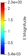
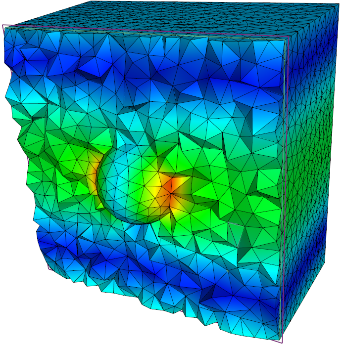
Figure 5. Representation of $|\boldsymbol{E}_{\rm r}(T)|$ in the scattering example.

To assess the impact of the postprocessing, we consider a set of evaluation points $\boldsymbol{A}$, and we compute relative errors

$$\text{err}(\boldsymbol{V})^{2}=\frac{\sum_{n=1}^{N}||\boldsymbol{\nabla}\times(\boldsymbol{V}_{\rm r}(t_{n},\boldsymbol{A})-\boldsymbol{V}_{h,n}(\boldsymbol{A}))||^{2}}{\sum_{n=1}^{N}||\boldsymbol{\nabla}\times(\boldsymbol{V}_{\rm r})(t_{n},\boldsymbol{A})||^{2}}$$

and

$$\text{err}^{\star}(\boldsymbol{V})^{2}=\frac{\sum_{n=1}^{N}||\boldsymbol{\nabla}\times(\boldsymbol{V}_{\rm r}(t_{n},\boldsymbol{A})-\boldsymbol{V}_{h,n}^{\star}(\boldsymbol{A}))||^{2}}{\sum_{n=1}^{N}||\boldsymbol{\nabla}\times(\boldsymbol{V}_{\rm r})(t_{n},\boldsymbol{A})||^{2}}$$

with $\boldsymbol{V}:=\boldsymbol{E}$ or $\boldsymbol{H}$. Table 5 shows that our postprocessing approach reduces the error by at least a factor of $2$ for the 9 evaluation points that we have selected.

Point	Field	err   $\text{err}^{\star}$
	$\boldsymbol{E}$	0.083  0.033
$A_{1}(0,0,0.45)$	$\boldsymbol{H}$	0.103  0.048
	$\boldsymbol{E}$	0.008  0.005
$A_{2}(0.2,-0.3,0.8)$	$\boldsymbol{H}$	0.008  0.006
	$\boldsymbol{E}$	0.019  0.005
$A_{3}(0.2,-0.3,0.2)$	$\boldsymbol{H}$	0.020  0.006
	$\boldsymbol{E}$	0.015  0.004
$A_{4}(0.2,0.3,0.2)$	$\boldsymbol{H}$	0.017  0.005
	$\boldsymbol{E}$	0.019  0.007
$A_{5}(0.2,0.3,0.8)$	$\boldsymbol{H}$	0.027  0.007
	$\boldsymbol{E}$	0.015  0.008
$A_{6}(-0.2,-0.3,0.8)$	$\boldsymbol{H}$	0.014  0.008
	$\boldsymbol{E}$	0.027  0.008
$A_{7}(-0.2,-0.3,0.2)$	$\boldsymbol{H}$	0.028  0.008
	$\boldsymbol{E}$	0.021  0.007
$A_{8}(-0.2,0.3,0.2)$	$\boldsymbol{H}$	0.024  0.007
	$\boldsymbol{E}$	0.010  0.005
$A_{9}(-0.2,0.3,0.8)$	$\boldsymbol{H}$	0.011  0.005

Table 5. Scattering of a plane wave by a dielectric sphere: $L^{2}$ error between the reference solution and the solution with a $\boldsymbol{\mathcal{P}}_{2}$ interpolation with and without applying the postprocessing.

5. Conclusion

In this work we have presented a postprocessing approach for a discontinuous Galerkin discretization of the time-dependent Maxwell’s equations in 3D. This postprocessing technique is inexpensive, and can be computed independently in each element of the mesh, and at every time step of interest. It is thus well adapted to parallel computer architectures. Moreover, it is particularly suited to applications requiring a higher accuracy in localized regions, either in time or space. We have presented numerical examples, both with analytical solution and in complicated geometries, that indicate that our postprocessing approach improves the convergence rate of the discrete solution in the $H(\operatorname{curl})$-norm by one order. Overall, this contribution is to be employed as an efficient way of reducing the $H(\operatorname{curl})$-norm error of discontinuous Galerkin discretizations.

References

- [1] R. Abgrall and C.W. Shu, Handbook of numerical methods for hyperbolic problems, vol. 17, Elsevier/North-Holland, Amsterdam, 2016.
- [2] A. B. Andreev and R. D. Lazarov, Superconvergence of the gradient for quadratic triangular finite elements, Numer. Methods for PDEs 4 (1988), 15–32.
- [3] D.N. Arnold, F. Brezzi, B. Cockburn, and L.D. Marini, Unified analysis of discontinuous Galerkin, methods for elliptic problems, SIAM J. Numer. Anal. 39 (2002), no. 5, 1749–1779.
- [4] F. Assous, P. Ciarlet, and S. Labrunie, Mathematical foundations of computational electromagnetism, Springer, 2018.
- [5] I. Babuska, T. Strouboulis, C. S. Upadhyay, and S. K. Gangaraj, Validation of recipes for the recovery of stresses and derivatives by a computer-based approach, Math. Comput. Mode. 20 (1994), 45.
- [6] by same author, Computer-based proof of the existence of superconvergence points in the finite element method; superconvergence of the derivatives in finite element solutions of laplace’s, poisson’s and the elasticity equations, Numer. Methods for PDEs 12 (1996), 347–392.
- [7] A. Bondeson, T. Rylander, and P. Ingelström, Computational Eelectromagnetics, Springer-Verlag, 2013.
- [8] M.H. Carpenter and C.A. Kennedy, Fourth-order 2N-storage Runge-Kutta schemes, NASA 109112 (1994).
- [9] P. Castillo, B. Cockbrn, I. Perugia, and D. Schötzau, An a priori error analysis of the local discontinuous Galerkin method for elliptic problems, SIAM J. Numer. Anal. 38 (2000), no. 5, 1676–1706.
- [10] P.G. Ciarlet, The finite element method for elliptic problems, SIAM, 2002.
- [11] L. Fezoui, S. Lanteri, S. Lohrengel, and S. Piperno, Convergence and stability of a discontinuous Galerkin time-domain method for the 3D heterogeneous Maxwell equations on unstructured meshes, ESAIM Math. Model. Numer. Anal. 39 (2005), no. 6, 1149–1176.
- [12] S.V. Gaponenko, Introduction to nanophotonics, Cambridge University Press, 2010.
- [13] G. Goodsell and J. R. Whiteman, A unified treatment of superconvergent recovered gradient functions for piecewise linear finite element approximations, Internat. J. Numer. Methods. Eng. 27 (1989), 469–481.
- [14] D.J. Griffiths, Introduction to Electrodynamics, Prentice Hall, 1999.
- [15] T. Hagstrom and S. Lau, Radiation boundary conditions for Maxwell’s equations: A review of accurate time-domain formulations, J. Comput. Math. 25 (2007), no. 3, 305–336.
- [16] J Hesthaven and T. Warburton, Nodal high-order methods on unstructured grids. I. Time-domain solution of Maxwll’s equations, J. Comput. Phys. 181 (2002), no. 1, 186–221.
- [17] P. Russer, Electromagnetics, microwave circuit and antenna design for communications engineering, Artech house, 2006.
- [18] M. Stanglmeier, N. Nguyen, J. Peraire, and B. Cockburn, An explicit hybridizable discontinuous Galerkin method for the acoustic wave equation, Comput. Meth. Appl. Mech. Engrg. 300 (2016), 748–769.
- [19] J. Viquerat, Simulation of electromagnetic waves propagation in nano-optics with a high-order discontinuous Galerkin time-domain method, Ph.D. thesis, Université Nice Sophia-Antipolis, 2015.
- [20] K. Yee, Numerical solution of initial boundary value problems involving Maxwell’s equations in isotropic media, IEEE Trans. Antennas Propag. 16 (1966), 302–307.