The role of energy in ballistic agglomeration

Abstract

We study a ballistic agglomeration process in the reaction-controlled limit. Cluster densities obey an infinite set of Smoluchowski rate equations, with rates dependent on the average particle energy. The latter is the same for all cluster species in the reaction-controlled limit and obeys an equation depending on densities. We express the average energy through the total cluster density that allows us to reduce the governing equations to the standard Smoluchowski equations. We derive basic asymptotic behaviors and verify them numerically. We also apply our formalism to the agglomeration of dark matter.

I Introduction

In aggregation, clusters merge irreversibly upon collisions. Aggregation is ubiquitous in Nature with applications ranging from Brownian coagulation Smoluchowski (1917); Family et al. (1985); Ball et al. (1987); Thorn and Seesselberg (1994); Odriozola et al. (2001, 2004) and polymerization Flory (1953) to atmospheric phenomena Hidy and Brock (1970); Drake (1972); Shrivastava (1982); Friedlander (2000) and astrophysical systems Field and Saslaw (1965); Lissauer (1993); Chokshi et al. (1993); Dominik and Tielens (1997); Ossenkopf (1993); Spahn et al. (2004); Esposito (2006); Brilliantov et al. (2015); Hardy et al. (2015); Krnjaic and Sigurdson (2015); Gresham et al. (2018). A complete description of aggregation is very complicated. A spectacular example of merging massive black holes has been studied theoretically, numerically, and experimentally; this is a very complicated process. Still, the details of the merging processes in ordinary phenomena like Brownian coagulation could be as complicated as in the black holes or neutron stars merging. Moreover, the mass spectrum is very broad. Hence the merging is usually modeled just postulating that it occurs with a certain rate depending on the parameters of the merging clusters. Clusters are also simply modeled by a single number, the mass of the cluster. Clusters are often built from minimal-mass entities, the monomers. In this situation the mass spectrum $m_{k}=m_{1}k$ is parametrized by integers $k=1,2,\ldots$.

The transport mechanism plays a crucial role in aggregation. In earlier applications of aggregation to Brownian coagulation, polymerization, and other physical and chemical processes, diffusion is the dominant transport mechanism, e.g. Family et al. (1985); Ball et al. (1987); Thorn and Seesselberg (1994); Odriozola et al. (2001, 2004). Thus the particles have random rather than deterministic trajectories. Such aggregation processes are well understood Leyvraz (2003); Krapivsky et al. (2010). The main quantities of interest are cluster densities $n_{k}(t)$ which depend only on the mass $k$ and time $t$. In the homogeneous setting, these densities evolve according to Smoluchowski rate equations. For infinite systems, Smoluchowski’s equations are an infinite system of nonlinear coupled ordinary differential equations depending on merging rates. Smoluchowski equations have been analytically solved only in a few cases, namely for the general bilinear kernel Drake (1972); Spouge (1983); more recently, exact solutions have been established for the parity kernel Calogero and Leyvraz (2000) and the $q$-sum kernel Calogero and Leyvraz (1999). Scaling analysis van Dongen and Ernst (1985, 1988) often provides a good qualitative understanding of the most interesting large time behavior.

Ballistic transport also underlies many aggregation processes such as aggregation of dust in interplanetary space and particles in planetary rings Chokshi et al. (1993); Dominik and Tielens (1997); Ossenkopf (1993); Spahn et al. (2004); Esposito (2006); Brilliantov et al. (2015). Since diffusive transport is usually tacitly assumed when aggregation is mentioned, we shall use the term ballistic agglomeration (BA) to describe aggregation processes with ballistic transport. The BA processes have diverse applications ranging from in-space manufacturing to the evolution of the dark matter Hardy et al. (2015); Krnjaic and Sigurdson (2015); Gresham et al. (2018).

Despite numerous studies of the BA processes Carnevale et al. (1990); Trizac and Hansen (1995); Frachebourg (1999); Frachebourg et al. (2000a, b); Valageas (2009); Trizac and Krapivsky (2003); Brilliantov and Spahn (2006); Brilliantov et al. (2018); Midya and Das (2017); Paul and Das (2018); Singh and Mazza (2019, 2018), our understanding of such systems is much less complete than the understanding of the diffusion-driven aggregation. The key difference of the BA from diffusion-driven aggregation is the primary role of the kinetic energy which is partially lost in merging events. In aggregation processes, each cluster is characterized by its mass; in the BA processes, we must also account for velocities and rely on a joint mass-velocity distribution satisfying Boltzmann-Smoluchowski equations Brilliantov and Spahn (2006); Brilliantov et al. (2009, 2015, 2018). The Boltzmann equation is already notoriously difficult; the Boltzmann-Smoluchowski equations form an infinite set of nonlinear coupled integro-differential equations, each one more complicated than the Boltzmann equation. One very general solution of the Boltzmann equation, the Maxwell distribution, describes equilibrium. If different cluster species were at equilibrium, then velocity distributions would be known. Temperature equilibrium (temperature equipartition) is violated for the BA: The temperatures of each species defined via the corresponding average kinetic energy are different.

Fortunately, there is a special limit when all species are close to temperature equilibrium. This is the reaction-controlled limit Trizac and Krapivsky (2003) (see also Ball et al. (1987); Thorn and Seesselberg (1994); Odriozola et al. (2001, 2004) for the diffusive transport) when, in contrast to the collision-controlled limit, merging occurs in a tiny fraction of collisions — clusters mostly undergo elastic collisions and therefore are near equilibrium. The entire system is then characterized by the same temperature $T(t)$; it evolves in time, manifesting the non-equilibrium nature of the process. An important feature of the reaction-controlled BA is the validity of the mean-field description; in the collision-controlled BA, the mean-field Boltzmann-Smoluchowski fails in all spatial dimensions Krapivsky et al. (2010) although the failure becomes pronounced only at a very large time and at intermediate times the deviations are usually small.

Previous work Trizac and Krapivsky (2003) on the reaction-controlled BA was focused on average quantities. In this paper, we develop a general framework that allows one to determine both the mass distribution and the evolution of temperature. This framework is presented in Sect. II. In Sect. III we apply our formalism to the agglomeration of dark matter. We conclude in Sect. IV.

II Rate equations for ballistic aggregation

II.1 Derivation of the rate equations

Equations governing the dynamics of the BA are derived in the realm of the Boltzmann equation Chapman and Cowling (1970); Brilliantov and Pöschel (2004) approach. The main object is $f_{k}(v_{k},t)$, the density of clusters of mass $k$ and velocity ${\bf v}_{k}$. To illustrate the basic physics, we provide a transparent derivation based on the direct computation of the collision rates and energy losses. We consider diluted and spatially uniform 3D systems. We ignore the shape of clusters and effectively assume that clusters are balls: a cluster of ‘size’ $k$ has mass $m_{k}=m_{1}k$ and the diameter $\sigma_{k}=\sigma_{1}k^{1/3}$.

To determine the merging rate consider a collision of two clusters with mass-velocity parameters $(i,{\bf v}_{i})$ and $(j,{\bf v}_{j})$. In the coordinate system attached to $(i,{\bf v}_{i})$, another cluster moves with the velocity ${\bf v}_{ij}={\bf v}_{i}-{\bf v}_{j}$. When projected onto the plane, perpendicular to the velocity ${\bf v}_{ij}$, the position of the second cluster can be specified in the polar coordinates by the radius $b$ (the impact parameter) and the polar angle $\phi$, see Fig. 1. Take clusters of mass $i$ with velocities in the tiny region of volume $d{\bf v}_{i}$ around ${\bf v}_{i}$; similarly for clusters of mass $j$. The number of collisions between such ensembles of clusters happening during the time interval $\Delta t$ in a small volume $d{\bf r}$ reads

$$f_{i}(v_{i})d{\bf v}_{i}\,f_{j}(v_{j})d{\bf v}_{j}\,v_{ij}\Delta t\,bd\phi db\,d{\bf r}\,.$$ (1)

The densities $f_{i}(v_{i})$ and $f_{j}(v_{j})$ do not depend on the spatial location (we consider only spatially uniform systems) and on the direction of the velocity (due to isotropy). The factor $bd\phi dbv_{ij}\Delta t$ gives the volume of the collision cylinder [see Fig. 1] specified by the impact parameter $b\in[b,b+db]$ and the angle $\phi$: $bd\phi db$ is the cross-section and $v_{ij}\Delta t$ is the length of the cylinder. Equation (1) is based on the assumption that the velocities of colliding clusters are uncorrelated. This assumption, first applied to molecular gases, was called a “molecular chaos hypothesis”. Here it is applied to particle physics and is expected to be accurate for diluted systems in the reaction-controlled setting. The use of the molecular chaos hypothesis in the collision-controlled setting is not completely justified.

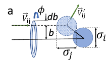
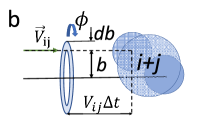
Figure 1: Sketch of the bouncing (a) and aggregative impact (b) of clusters of size $i$ and $j$. The collision is specified by the impact parameter $b$, the angle $\phi$, and the relative velocity $v_{ij}$.

To find the number of collisions between clusters of size $i$ and $j$ we integrate (1) over parameters specifying the collision, that is, over $\phi\in[0,2\pi]$ and $b\in[0,\sigma_{ij}]$ with $\sigma_{ij}=(\sigma_{i}+\sigma_{j})/2$, and also over all possible velocities ${\bf v}_{i}$ and ${\bf v}_{j}$. The agglomeration rate is therefore

$${\cal B}_{ij} = \int_{0}^{2\pi}\!\!d\phi\int_{0}^{\sigma_{ij}}bdb\int d{\bf v}_{i}\,f_{i}(v_{i})\int d{\bf v}_{j}\,f_{j}(v_{j})v_{ij}$$ (2)

$$= \pi\sigma_{ij}^{2}\int\int d{\bf v}_{i}\,d{\bf v}_{j}\,v_{ij}f_{i}(v_{i})f_{j}(v_{j})\,.$$

In the reaction-controlled limit, a tiny fraction of collisions leads to merging. We assume for simplicity that this fraction does not depend on the cluster size and/or on the relative velocity of the collision, although generally, this could be violated, see e.g. Odriozola et al. (2001, 2004). With this assumption, we can put the fraction into the time variable to avoid cluttering the formulae.

Since almost all collisions are like in the classical gas, the velocity distribution functions are Maxwellian: $f_{i}(v_{i})=n_{i}e^{-v_{i}^{2}/v_{0,i}^{2}}/(\pi^{3/2}v_{0,i}^{3})$, where $n_{i}$ is the number density of clusters of size $i$ and $v_{0,i}=\sqrt{2T/m_{i}}$ is the thermal velocity of such clusters ($T$ is the temperature measured in the units of energy; equivalently, we set the Boltzmann constant to unity).

To compute the integral in Eq. (2) we first make the transformation, $({\bf v}_{i},{\bf v}_{j})\to({\bf V},{\bf v}_{ij})$, to the center of mass velocity ${\bf V}=(m_{i}{\bf v}_{i}+m_{j}{\bf v}_{j})/(m_{i}+m_{j})$ and the relative velocity ${\bf v}_{ij}={\bf v}_{i}-{\bf v}_{j}$. The product of the velocity distribution functions becomes

$$f_{i}(v_{i})f_{j}(v_{j})=\frac{n_{i}n_{j}}{\pi^{3}v_{0,i}^{3}v_{0,j}^{3}}\,\exp\!\left[-\frac{\mu_{ij}v_{ij}^{2}+(m_{i}+m_{j})V^{2}}{2T}\right]$$

where $\mu_{ij}=m_{i}m_{j}/(m_{i}+m_{j})$ is the reduced mass. Inserting this expression into (2) and using the identity $d{\bf v}_{i}d{\bf v}_{j}=d{\bf V}d{\bf v}_{ij}$ we get a product of two Gaussian integrals. Computing the integrals we find that the agglomeration rates are proportional to $\sqrt{T}$:

$${\cal B}_{ij}=\sqrt{T}\,K_{ij}n_{i}n_{j}\,.$$ (3)

The mass-dependent factor of the rates is given by

$$K_{ij}=K_{0}(i^{1/3}+j^{1/3})^{2}\sqrt{i^{-1}+j^{-1}},$$ (4)

where $K_{0}=\sigma_{1}^{2}\sqrt{\pi/(2m_{1})}$; see Brilliantov et al. (2009, 2015, 2018) for details of such calculations. The governing equations for the densities are the Smoluchowski equations

$$\frac{dn_{k}}{dt}=T^{1/2}\left[\frac{1}{2}\sum_{i+j=k}K_{ij}n_{i}n_{j}-n_{k}\sum_{i\geq 1}K_{ki}n_{i}\right]$$ (5)

with a temperature-dependent factor.

Next, we derive the evolution equation for the total kinetic energy density, $\frac{3}{2}nT$, where $n=\sum_{k\geq 1}n_{k}$ is the total cluster density. In a collision between clusters $i$ and $j$ leading to merging, the total energy of the pair is reduced by the energy of the relative motion of the pair, $\mu_{ij}v_{ij}^{2}/2$. We treat the merged cluster as a single entity and thus do not account for the kinetic energy of the inner motion, which remains after the collision. To obtain the rate equation for the decay of the energy $\frac{3}{2}nT$, we multiply the integrand in Eq. (2) by $\mu_{ij}v_{ij}^{2}/2$, integrate over all possible velocities ${\bf v}_{i}$ and ${\bf v}_{j}$, and sum over all $i$ and $j$. This gives the energy equation

$$\frac{d}{dt}nT=-\frac{2}{3}\,T^{3/2}\sum_{i\geq 1}\sum_{j\geq 1}K_{ij}n_{i}n_{j}\,.$$ (6)

We ignore the energy loss in the bouncing collisions. Hence these elastic collisions do not contribute to the evolution of the kinetic energy in (6). The generalization for inelastic collisions (as in granular gases Brilliantov and Pöschel (2004)) is straightforward but would complicate the notations.

II.2 Analysis of the rate equations

Summing Eqs. (5) yields

$$\frac{dn}{dt}=-\frac{1}{2}\,T^{1/2}\sum_{i\geq 1}\sum_{j\geq 1}K_{ij}n_{i}n_{j}\,.$$ (7)

Massaging (6) and (7) we obtain a neat result

$$\frac{dT}{dn}=\frac{1}{3}\,\frac{T}{n}$$ (8)

implying that the temperature is a purely algebraic function of the total density:

$$T(t)/T(0)=\left[n(t)/n(0)\right]^{1/3}\,.$$ (9)

We emphasize that Eq. (8) holds independently of such details as the shape of clusters or the fraction of the aggregation events (which can also depend on cluster sizes). However, one still needs to assume a complete elasticity of the bouncing collisions and that the fraction of merging events does not depend on the collision speeds.

We can absorb the factor $\sqrt{T}$ in Eqs. (5) into the time variable by introducing the modified time

$$\tau=\int_{0}^{t}dt^{\prime}\,\sqrt{T(t^{\prime})}\,.$$ (10)

The corresponding Smoluchowski equations

$$\frac{dn_{k}}{d\tau}=\frac{1}{2}\sum_{i+j=k}K_{ij}n_{i}n_{j}-n_{k}\sum_{i\geq 1}K_{ki}n_{i}$$ (11)

with rates (4) are analytically intractable. Fortunately, the rates (4) are homogeneous, namely they satisfy

$$K_{si,sj}=s^{\lambda}K_{i,j}\,.$$ (12)

For rates (4), the homogeneity index is $\lambda=1/6$. The scaling approach van Dongen and Ernst (1985); Krapivsky et al. (2010) tells us that the total density decays as $n\sim\tau^{-1/(1-\lambda)}$, so in the present case $n\sim\tau^{-6/5}$. Using this asymptotic together with (9)–(10) we obtain

$$t\sim\int_{0}^{\tau}d\tau^{\prime}\,[T(\tau^{\prime})]^{-1/2}\sim\int_{0}^{\tau}d\tau^{\prime}\,[n(\tau^{\prime})]^{-1/6}\sim\tau^{6/5}$$

implying that

$$n\sim t^{-1}\,,\quad\qquad T\sim t^{-1/3}\,.$$ (13)

The scaling approach further predicts van Dongen and Ernst (1985); Leyvraz (2003); Krapivsky et al. (2010) that the cluster-mass distribution approaches a scaling form

$$n_{k}=n^{2}\Phi(kn)$$ (14)

in the scaling limit $t\to\infty$ ($\tau\to\infty$), $k\to\infty,~{}kn=\text{finite}$. Here $n_{k}$ and $n$ depend either on $t$ or $\tau$; that is, the scaling distribution $\Phi(x)$ is universal. Figure 2 illustrates that for the temperature-dependent agglomeration, (5)–(6), the distribution $\Phi(x)$ quickly settles and coincides with the one for the standard Smoluchowski equations.

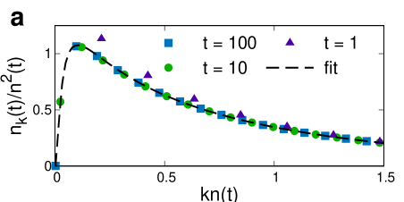
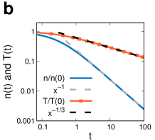
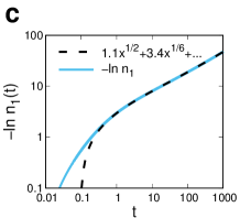
Figure 2: (a) The reduced density distribution $n_{k}(t)/n^{2}(t)$ as a function of $kn(t)$ for different times for the 3D system ($n(0)=T(0)=K_{0}=1$). The convergence to the scaled distribution $\Phi(x)$ with $x=kn(t)$ is observed already at $t=10$. The scaled distribution is well fit by $\left(\frac{0.785}{x^{0.28}}+\frac{0.65}{x}\right)e^{-0.61/\sqrt{x}-0.81x}$. (b,c) The time dependence of temperature, the total density and monomer density. Solid lines are numerical results; dashed lines are the asymptotic predictions, Eqs. (13) and (16). The data presented in (a) and (c) are obtained by numerically solving ordinary differential equations (ODEs). The data in (b) are from Monte-Carlo simulations (see Appendix A for detail).

The behavior of the scaled mass distribution $\Phi(x)$ depends on homogeneity indexes $\mu$ and $\nu$ defined via

$$K_{i,j}\sim i^{\mu}j^{\nu}\quad\text{when}\quad j\gg i\,.$$ (15)

Thus $\lambda=\mu+\nu$ and the reaction rates satisfying (12) and (15) are characterized by two independent homogeneity indexes. For such homogeneous rates, qualitative behaviors are understood, see van Dongen and Ernst (1985, 1988); Connaughton et al. (2017, 2018); it greatly depends on whether the index $\mu$ is larger or smaller than zero. Reaction rates with $\mu<0$ are known as type III rates van Dongen and Ernst (1985). The mass distribution in this case is bell-shaped van Dongen and Ernst (1985, 1988), with an exponential decay in the large mass limit, and stretched exponential decay $\ln[1/\Phi(x)]\sim x^{-|\mu|}$ in the small mass limit.

For reaction rates (4) are of type III, the indexes are $\mu=-\frac{1}{2}$ and $\nu=2/3$. Adopting the treatment of Ref. van Dongen and Ernst (1988) one can deduce a rather precise decay law

$$-\ln[n_{1}(t)/n(0)]=C_{1}t^{1/2}+C_{2}t^{1/6}+O(1)$$ (16)

for the density of monomers as we explain below.

II.3 Ballistic aggregation: General dimension

The generalization of Eqs. (5)–(6) to arbitrary spatial dimension $d$ is straightforward. The agglomeration rate is given by the same integral as in Eq. (2) multiplied by $\Omega_{d-1}\sigma_{ij}^{d-1}$ instead of the factor $\pi\sigma_{ij}^{2}$ for the 3D systems. Here $\Omega_{d}=\pi^{d/2}/\Gamma(1+d/2)$ is the volume of a unit $d$-dimensional ball. Then one derives Eqs. (5) with mass-dependent rates

$$K_{ij}=K_{0}(i^{1/d}+j^{1/d})^{d-1}\sqrt{i^{-1}+j^{-1}}\,.$$ (17)

Since the loss of energy in collisions is the same as in three dimensions, $\frac{1}{2}\mu_{ij}v_{ij}^{2}$, the energy equation becomes

$$\frac{d}{dt}nT=-\frac{d+1}{2d}\,T^{3/2}\sum_{i\geq 1}\sum_{j\geq 1}K_{ij}n_{i}n_{j}\,,$$ (18)

where we have taken into account that $(d/2)nT$ gives the total kinetic energy in the $d$-dimensional case.

Using Eqs. (5), (18) and repeating analysis that has led to Eq. (8) we derive

$$\frac{T(t)}{T(0)}=\left[\frac{n(t)}{n(0)}\right]^{1/d}\,.$$ (19)

The rates (17) are homogeneous, with homogeneity index $\lambda=(d-2)/(2d)$. The same analysis as in three dimensions gives the asymptotic decay laws

$$n\sim t^{-2d/(d+3)}\,,\qquad\quad T\sim t^{-2/(d+3)}\,.$$ (20)

The density of monomers in three dimensions decays according to Eq. (16) in the large time limit. We now derive this result, as well as the more general small mass asymptotic. We also outline a generalization to an arbitrary spatial dimension. Our derivation adopts the procedure developed in Ref. van Dongen and Ernst (1988). By inserting the scaling form (14) into the Smoluchowski equations (11) and using (17) we obtain

$$w[2\Phi(x)+x\Phi^{\prime}(x)] = \Phi(x)\int_{0}^{\infty}dy\,\Phi(y)\,K(x,y)$$

$$- \frac{1}{2}\int_{0}^{x}dy\,\Phi(y)\Phi(x-y)K(y,x-y)$$

where

$$\frac{dn}{d\tau}=-wn^{2-\lambda}\,,\qquad\lambda=\frac{1}{2}-\frac{1}{d}$$ (22a)

$$w=-\frac{1}{2}\int_{0}^{\infty}dx\int_{0}^{\infty}dy\,\Phi(x)\,\Phi(y)\,K(x,y)$$ (22b)

$$K(x,y)=K_{0}(x^{1/d}+y^{1/d})^{d-1}\sqrt{x^{-1}+y^{-1}}$$ (22c)

In the $y\to\infty$ limit, the kernel $K(x,y)$ admits an expansion

$$K(x,y)=\sum_{n\geq 0}K_{n}x^{\mu_{n}}y^{\lambda-\mu_{n}}$$ (23)

with $\mu_{0}=\mu=-\frac{1}{2}$ universal in all dimensions; $\mu_{1}=\frac{1}{d}-\frac{1}{2}$ and $K_{1}=(d-1)K_{0}$; $\mu_{2}=\frac{2}{d}-\frac{1}{2},~{}K_{1}=\frac{1}{2}(d-1)(d-2)K_{0}$ when $d>2$ and $\mu_{2}=\frac{1}{2},~{}K_{1}=\frac{1}{2}K_{0}$ when $d=2$; etc. Inserting (23) into (II.3) and focusing on the small mass behavior, $x\downarrow 0$, we find

$$w[2\Phi(x)+x\Phi^{\prime}(x)]\simeq\Phi(x)\sum_{n\geq 0}K_{n}x^{\mu_{n}}M_{\lambda-\mu_{n}}$$ (24)

where $M_{p}$ is the $p^{\text{th}}$ moment of the scaled mass distribution:

$$M_{p}=\int_{0}^{\infty}dy\,\Phi(y)\,y^{p}$$ (25)

Integrating Eq. (24) one obtains van Dongen and Ernst (1988)

$$\Phi(x)\sim x^{-2}\exp\!\left[\sum_{n\geq 0}\frac{K_{n}M_{\lambda-\mu_{n}}}{w\mu_{n}}\,x^{\mu_{n}}\right]$$ (26)

with sum running over such $n$ that $\mu_{n}<0$ if $\mu_{n}\neq 0$ for all $n$; if $\mu_{n}=0$ for some value $n$, the term $x^{\mu_{n}}/\mu_{n}$ should be replaced by $\ln x$.

Since $\mu_{0}=-\frac{1}{2},~{}\mu_{1}=-\frac{1}{6},\mu_{2}=\frac{1}{6}$ in three dimensions, Eq. (26) becomes

$$\Phi(x)\sim x^{-2}\exp\!\left[-A_{1}x^{-1/2}-A_{2}x^{-1/6}\right].$$ (27)

Thus $n_{1}=n^{2}\Phi(n)\sim\exp\!\left[A_{1}n^{-1/2}-A_{2}n^{-1/6}\right]$ leading to the announced asymptotic behavior (16) in three dimensions.

In two dimensions, $\mu_{0}=-\frac{1}{2}$ and $\mu_{1}=0$, so Eq. (26) yields $n_{1}\sim\exp\!\left[-A_{1}n^{-1/2}-A_{2}\ln n\right]$, from which

$$-\ln\frac{n_{1}(t)}{n(0)}\sim C_{1}t^{\frac{2}{5}}+C_{2}\ln t+O(1)$$ (28)

When $d=4$, we get $\mu_{0}=-\frac{1}{2},~{}\mu_{1}=-\frac{1}{4}$ and $\mu_{2}=0$, from which

$$-\ln\frac{n_{1}(t)}{n(0)}\sim C_{1}t^{\frac{4}{7}}+C_{2}t^{\frac{2}{7}}+C_{3}\ln t+O(1)$$ (29)

The constants $C_{1},~{}C_{2}$ etc. appearing in Eqs. (16), (28) are different, even if denoted by the same letter. These constants are unknown as they depend on the moments of the scaled mass distribution which are analytically unknown.

Thus the monomer density exhibits the stretched exponential decay

$$\ln\frac{n_{1}(t)}{n(0)}\sim-t^{\frac{d}{d+3}}$$ (30)

in the leading order. The leading behavior of the mass distribution in the small mass limit is

$$\ln\frac{n_{k}(t)}{n(0)}\sim-k^{-\frac{1}{2}}t^{\frac{d}{d+3}}\qquad\quad\text{for}\qquad\quad k\ll t^{\frac{2d}{d+3}}\,.$$ (31)

In Fig. 3 we present the density distribution and asymptotic behavior for $n(t)$ and $T(t)$ for two-dimensional systems.

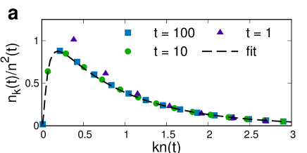
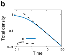
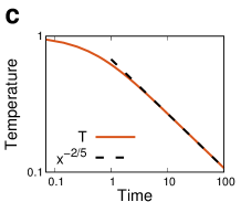
Figure 3: (a) The reduced density distribution $n_{k}(t)/n^{2}(t)$ as a function of $kn(t)$ for different time $t$ for 2D system. The convergence to the scaling function $\Phi(x)$ with $x=kn(t)$ is observed already at $t=10$. The scaled mass distribution $\Phi(x)$ is well fit by $\left(\frac{2.13}{x^{0.25}}+\frac{1.03}{x^{1.28}}\right)e^{-1.05/\sqrt{x}-1.035x}$. (b,c) The time dependence of the total density and temperature. Solid lines — numerical results; dashed lines — theoretical predictions, Eqs. (20) for $d=2$. (a) and fit function are from the ODE solution; (b) and (c) are from Monte-Carlo simulations (see Appendix A for detail).

III Ballistic aggregation: Application to dark matter

For many years, dark matter was thought of as a single stable and weakly interacting particle, but this paradigm is being challenged by a wider view where dark matter is part of a larger dark sector. In this framework, the formation of dark nuclei with a very wide spectrum of masses becomes plausible. The agglomeration of dark nuclei from dark nucleons has been studied in Hardy et al. (2015); Krnjaic and Sigurdson (2015); Gresham et al. (2018). In our framework, the governing equations are (5)–(6), with replacement $\frac{d}{dt}\to\frac{d}{dt}+3H$, where $H=H(t)$ is the Hubble parameter accounting for the expansion of the Universe. The transformation

$$n_{k}=hm_{k},\qquad h(t)=\exp\!\left[-3\int_{t_{0}}^{t}dt^{\prime}\,H(t^{\prime})\right]$$ (32)

recasts these equations into

$$\frac{1}{hT^{1/2}}\frac{dm_{k}}{dt}\!\! = \!\!\frac{1}{2}\!\!\sum_{i+j=k}\!\!K_{ij}m_{i}m_{j}\!-\!m_{k}\!\sum_{i\geq 1}\!K_{ki}m_{i}$$ (33)

$$\frac{1}{hT^{3/2}}\frac{d\,mT}{dt}\!\! = \!\!-\frac{2}{3}\sum_{i\geq 1}\sum_{j\geq 1}K_{ij}m_{i}m_{j}$$ (34)

that differ from (5)–(6) only by an extra factor $h(t)$. In Ref. Hardy et al. (2015) it was assumed that the dark nuclei were in contact with a bath of lighter particles, which determined their temperature. The temperature of the bath was gradually decreasing during the evolution of the Universe. Here we only take into account collisions between dark nuclei, so the temperature is defined by the agglomeration and Hubble expansion only; that is the system of dark nucleons is assumed to be completely isolated.

Agglomeration begins at sufficiently low temperatures, say when the temperature drops below $T_{0}$. Initially, the temperature decreases mainly due to radiation, which is especially important at high temperatures in the early stages of the Universe. However, we assume that at $T=T_{0}$ this type of energy loss is already quite slow, so that the aggregation quickly becomes dominant when it starts. In the definition (32) of $h(t)$ we set the lower limit $t_{0}$ as the time when this occurs, $T_{0}=T(t_{0})$. The natural initial condition is $m_{k}(t_{0})=n_{0}\delta_{k,1}$, where $n_{0}=n(t_{0})$. Using (33)–(34) we find that for $t\geq t_{0}$ the temperature and the auxiliary total density are related via

$$T(t)/T_{0}=\left[m(t)/n_{0}\right]^{1/3}.$$ (35)

We rescale $m_{k}\to n_{0}m_{k}$, $T\to T_{0}T$ and $K_{0}\to n_{0}T_{0}^{1/2}K_{0}$, where $K_{0}$ is defined by Eq. (4) and keep, for simplicity, the same notations for these quantities. Then with the dimensionless time

$${\cal T}=K_{0}\,\int_{t_{0}}^{t}dt^{\prime}\,h(t^{\prime})$$ (36)

we recast Eqs. (33)–(34) into the temperature-dependent Smoluchowski equations (5)–(6) for $m_{k}({\cal T})$, whose properties have been analyzed previously.

To determine $h(t)$, we need a bit of cosmology. There is solid observational evidence in favor of the flat Universe with positive cosmological constant $\Lambda$ representing dark energy. Then the Friedmann equation for the scaled factor $a(t)$ reads

$$\frac{\dot{a}^{2}}{a^{2}}=\frac{8\pi G\rho+\Lambda c^{2}}{3}\,.$$ (37)

Here $G$ is the Newton constant, $\rho$ the density, $c$ the speed of light and $H=a^{-1}\dot{a}$. Density $\rho$ can be determined from the Friedman acceleration equation

$$\frac{\ddot{a}}{a}=-\frac{4\pi G}{3}\left(\rho+\frac{3p}{c^{2}}\right)+\frac{\Lambda c^{2}}{3},$$ (38)

where $p$ is pressure. Combining (38) with (37) we find $\dot{\rho}=-\frac{3\dot{a}}{a}\left(\rho+p/c^{2}\right)$. If agglomeration of dark matter indeed occurs, it begins in the radiation dominated era of the expansion Hardy et al. (2015). At this stage the equation of state is $p=\rho c^{2}/3$ and from the previous equation for $\dot{\rho}$ one finds $\rho(t)/\rho_{0}=\left(a_{0}/a(t)\right)^{4}$. Using this result together with $\Lambda c^{2}\ll 8\pi G\rho$ which is valid in the radiation era, see Meehan and Whittingham (2015), we simplify Eq. (37) to

$$a\,\frac{da}{dt}=\sqrt{\frac{8\pi G\rho_{0}a_{0}^{4}}{3}}$$ (39)

Integrating (39), using Eq. (32) with $H=a^{-1}\dot{a}$ we find

$$h(t)=\left[1+2H_{0}(t-t_{0})\right]^{-3/2}$$ (40)

with $H_{0}=H(t_{0})=\left(8\pi G\rho_{0}/3\right)^{1/2}$. Equation (36) then yields

$${\cal T}(t)=\frac{K_{0}}{H_{0}}\left(1-\frac{1}{\sqrt{1+2H_{0}(t-t_{0})}}\right).$$ (41)

The modified time ${\cal T}$ remains finite and the agglomeration effectively ceases in the radiation-dominated era if $H_{0}(t_{r}-t_{0})\gg 1$.

If $t_{0}$ is close to the end of the radiation era $t_{r}$, the agglomeration continues for $t>t_{r}$. The freezing then occurs in the matter-dominated era, so one can use Meehan and Whittingham (2015)

$$a^{1/2}\,\frac{da}{dt}=\sqrt{\frac{8\pi G\rho_{0}a_{0}^{3}}{3}}.$$ (42)

Solving this equation one can find $H(t)=\dot{a}(t)/a(t)$ for the matter-dominated era, $h(t)$ and eventually ${\cal T}(t)$. The details of the derivation are presented in Appendix B, here we just quote the result:

$${\cal T}(t)=2K_{0}t_{0}\left[1-\sqrt{\frac{t_{0}}{t_{r}}}\left(\frac{3t_{r}+t}{3t+t_{r}}\right)\right]\,.$$ (43)

For simplicity, we have assumed a sharp transition from the radiation to matter-dominated era. Hence the modified time remains finite:

$${\cal T}<{\cal T}_{\max}=2K_{0}t_{0}\left(1-\sqrt{t_{0}/9t_{r}}\right).$$ (44)

The evolution thus freezes, and if ${\cal T}_{\max}$ is large enough, the modified densities, $m_{k}({\cal T})$, the frozen scaled form

$$m_{k}^{\rm frozen}=m^{2}({\cal T}_{\rm max})\Phi\left[km({\cal T}_{\rm max})\right],$$ (45)

where the scaling function $\Phi(x)$ is the same as for the standard or temperature-dependent Smoluchowski equations. Evolution with the freezing has been also reported in Hardy et al. (2015). Figure 4 illustrates the convergence of $m_{k}$ to the frozen distribution (45) for increasing $t$ for two scenarios: the freezing within the radiation-dominated and matter-dominates eras.

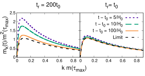
Figure 4: The modified densities $m_{k}(t)$ as a function of size $k$ for different agglomeration time $t-t_{0}$. For $t_{r}=200\,t_{0}$ the agglomeration ceases in the radiation-dominated era (left), while for $t_{0}=t_{r}$ – in the matter-dominated era (right). In both cases the distribution converges to the frozen one (45). The particular value $m({\cal T}_{\rm max})$ is determined by $K_{0}/H\simeq 2K_{0}t_{0}$, which is assumed to be large enough to guarantee scaling. Results are obtained by the ODE solution (see Appendix A).

IV Conclusion

We have investigated the ballistic agglomeration process in the reaction-controlled limit. Cluster densities satisfy an infinite set of Smoluchowski rate equations, with rates proportional $\sqrt{T}$, where $T$ is the kinetic temperature whose evolution is described by an energy equation. Remarkably, the temperature admits an expression through the total cluster density alone. In the reaction-controlled limit, the exponents describing the evolution of the total density and energy have been established in Ref. Trizac and Krapivsky (2003). Our more comprehensive description additionally gives the mass distribution. In particular, we have obtained an unexpected stretched exponential decay for the density of monomers. Our theoretical findings are in good agreement with simulation results.

We emphasize that the ballistic agglomeration process in the collision-controlled limit is not yet analytically understood in three dimensions, and generally when $d\geq 2$; the one-dimensional model is exactly solvable Frachebourg (1999); Frachebourg et al. (2000a, b); Valageas (2009). Some quantities exhibit drastically different behaviors in the reaction-controlled and collision-controlled cases. For instance, in one dimension the density of monomers decays as $\exp\!\left[-Ct^{1/4}\right]$ in the reaction-controlled case, while in the collision-controlled limit $n_{1}\sim t^{-1}$, that is the decay is much slower.

We have applied our formalism to the evolution of dark matter, namely to a model of asymmetric dark matter Hardy et al. (2015); Krnjaic and Sigurdson (2015); Gresham et al. (2018) where dark nuclei are formed via agglomeration of elementary dark nucleons. We have assumed that collision events rarely lead to merging. In this reaction-controlled limit, the system reaches the temperature equipartition for different cluster species without the need for the bath of light particles Hardy et al. (2015); Gresham et al. (2018). The size distribution of the dark nuclei tends to a final frozen distribution whose functional form follows from the solution of the standard Smoluchowski equations. A wide spectrum of masses calls for novel strategies for direct detection of heavy dark matter nuclei Coskuner et al. (2019). Among possible directions for future work, we mention symmetric dark matter models where the agglomeration should be supplemented by annihilation.

Appendix A Numerical methods

In our study we used two different numerical methods: the ODE solution and Monte-Carlo simulations. Both methods are popular and efficient tools to study the aggregation kinetics, see e.g. Family et al. (1985); Thorn and Seesselberg (1994); Odriozola et al. (2001, 2004).

Monte-Carlo simulations have been used to obtain the results for Fig. 2(b) and Fig. 3(b,c); it allows directly prove the validity of Eq. (19). The detail of the Monte-Carlo approach exploited here may be found in Refs. Bodrova et al. (2020); Osinsky et al. (2020). The only difference of the present implementation of this method is that the speeds of the particles were generated from the Maxwell distribution before each collision, without the use of a bath, as in Bodrova et al. (2020); Osinsky et al. (2020). This follows from the fact that the particles have time to exchange kinetic energy between the aggregation events. We used $10^{7}$ particles and doubled them every time when their number decreased by a factor of two.

In other figures (Fig. 2(a,c), Fig. 3(a), Fig. 4) we solved the ODE system (5)–(6) directly, after limiting the total number of equations to 50000. While Monte-Carlo and ODE method converge to the same solution, when the time step goes to zero and the number of particles goes to infinity, the ODE solution converges much faster and does not have stochastic noise. For better accuracy, we used second-order predictor-corrector scheme with an adaptive time step of $\tau=0.01$. In this case, the time step is calculated as

$$\Delta t_{k} =\tau\frac{\max\limits_{i}\left|n_{i}(t_{k-1})\right|}{\max\limits_{i}\left|n_{i}(t_{k-1})-n_{i}(t_{k})\right|},$$ (46)

$$t_{k+1} =t_{k}+\Delta t_{k}.$$

To speed up the solution of the ODE system, we used the method for generalized Smoluchowski equations Osinsky (2020), which is based on a low-rank approach from Matveev et al. (2014, 2017). The same solution can be obtained by solving the Smoluchowski equations directly like any other finite system of ODEs. However, the application of the low-rank approximation and adaptive time step technique accelerates the computations enormously Osinsky (2020); Matveev et al. (2014, 2017).

Appendix B Derivation of Eq. (43)

If the agglomeration starting time $t_{0}$ is close to the end of the radiation-dominated era, $t_{r}\approx 50000\text{ years}$, a significant number of collisions still happen for $t>t_{r}$ in the matter-dominated era. For $t>t_{r}$, the pressure becomes very small, so $\dot{\rho}=-\frac{3\dot{a}}{a}\left(\rho+p/c^{2}\right)$ reduces to $\dot{\rho}=-3(\dot{a}/a)\rho$.

Obviously, the transition from the state with the non-vanishing pressure $p_{r}$ in the radiation-dominated era to the state with $p\approx 0$ in the matter-dominated era is not instantaneous. The evolution of pressure for the transient period may be described (see Meehan and Whittingham (2015)) as

$$p\approx\frac{p_{r}}{1+T_{eq}/T}\,,$$

where $T_{eq}$ is the temperature of matter-radiation equilibrium. This makes the analysis of the transient period extremely complicated and does not allow us to obtain an explicit relation for the modified time $\tau$. Therefore, for the qualitative analysis, we assume that the transition period is short enough, as compared to the total time of the formation of the density distribution of dark matter. Hence we effectively postulate that this transition is instantaneous. Combining $\rho(t)/\rho(t_{r})=\left(a(t_{r})/a(t)\right)^{3}$ and Eq. (37) we obtain

$$a^{1/2}\,\frac{da}{dt}=\sqrt{\frac{8\pi G\rho_{r}a_{r}^{3}}{3}}$$ (47)

for $t>t_{r}$, where $\rho_{r}$ and $a_{r}$ are the quantities at the end of the radiation-dominated era. This equation is solved to yield the behavior $H(t)=\dot{a}(t)/a(t)$ for the matter-dominated era. The quantity $h(t)$ defined in Eq. (32) reads

$$h(t)=h_{r}\left[1+\frac{3}{2}H_{r}\left(t-t_{r}\right)\right]^{-2},\qquad t>t_{r},$$ (48)

where $H_{r}=H(t_{r})$ and $h_{r}=h(t_{r})$ are again the quantities at the end of the radiation-dominated era. Note that one can ignore the cosmological constant $\Lambda$ which becomes relevant only when the Universe is older than about 10 billion years.

To determine the modified time ${\cal T}$ for $t>t_{r}$ we first need to find ${\cal T}(t_{r})$ from Eq. (47) and then add the corresponding integral with $h(t)$ given by Eq. (48). To simplify the computations, let us assume that $t_{0}$ is far from cosmic inflation (otherwise, everything would have already aggregated in radiation-dominated era). Then since $a(t)\sim t^{1/2}$, as it follows from Eq. (39) we obtain the estimates for the beginning of the agglomeration and the end of the radiation era:

$$H_{0}=\frac{\dot{a}(t_{0})}{a_{0}}\simeq\frac{1}{2t_{0}}\,,\qquad H_{r}\simeq\frac{1}{2t_{r}}$$ (49)

Then we arrive at

$${\cal T}(t) = {\cal T}(t_{r})+\left[{\cal T}(t)-{\cal T}(t_{r})\right]$$

$$= \frac{K_{0}}{H_{0}}\left(1-\frac{1}{\sqrt{1+2H_{0}\left(t_{r}-t_{0}\right)}}\right)+\int_{t_{r}}^{t}dt^{\prime}\,{K_{0}}h(t^{\prime})$$

Massaging this expression we simplify it to

$${\cal T}(t) \simeq 2K_{0}t_{0}\left(1-\sqrt{\frac{t_{0}}{t_{r}}}\right)$$

$$+ \frac{4{K_{0}}t_{r}}{3}\left(\frac{t_{0}}{t_{r}}\right)^{3/2}\left(1-\frac{1}{1+\frac{3}{4t_{r}}\left(t-t_{r}\right)}\right)$$

$$= 2K_{0}t_{0}\left[1-\sqrt{\frac{t_{0}}{t_{r}}}\left(\frac{3t_{r}+t}{3t+t_{r}}\right)\right].$$

This completes the derivation of Eq. (43). In the long time limit, one can further simplify to obtain Eq. (44).

Acknowledgments. This study has been supported by RFBR through the research projects №18-29-1919 and №20-31-90022.

References

- Smoluchowski (1917) M. V. Smoluchowski, Z. Phys. Chem. 92, 129 (1917).
- Family et al. (1985) F. Family, P. Meakin, and T. Vicsek, J. Chem. Phys. 83, 4144 (1985).
- Ball et al. (1987) R. C. Ball, D. A. Weitz, T. A. Witten, and F. Leyvraz, Phys. Rev. Lett. 58, 274 (1987).
- Thorn and Seesselberg (1994) M. Thorn and M. Seesselberg, Phys. Rev. Lett. 72, 3622 (1994).
- Odriozola et al. (2001) G. Odriozola, A. Moncho-Jordá, A. Schmitt, J. Callejas-Fernández, R. Martínez-García, and R. Hidalgo-Álvarez, Europhys. Lett. 53, 797 (2001).
- Odriozola et al. (2004) G. Odriozola, R. Leone, A. Schmitt, J. Callejas-Fernández, R. Martínez-García, and R. Hidalgo-Álvarez, J. Chem. Phys. 121, 5468 (2004).
- Flory (1953) P. J. Flory, Principles of Polymer Chemistry (Cornell University Press, 1953).
- Hidy and Brock (1970) G. R. Hidy and J. R. Brock, The Dynamics of Aerocolloidal Systems, International Reviews in Aerosol Physics and Chemistry (Pergamon Press, Oxford, 1970).
- Drake (1972) R. L. Drake, In: G. M. Hidy, and J. R. Brock (Eds.), Topics in Current Aerosol Research, Vol. 3, part 2 (Pergamon Press, New York, 1972).
- Shrivastava (1982) R. C. Shrivastava, J. Atom. Sci. 39, 1317 (1982).
- Friedlander (2000) S. K. Friedlander, Smoke, Dust and Haze, 2nd Edition (Oxford University Press, Oxford, 2000).
- Field and Saslaw (1965) G. B. Field and W. C. Saslaw, Astrophys. J 142, 568 (1965).
- Lissauer (1993) J. J. Lissauer, Ann. Rev. Astron. Astrophys. 31, 129 (1993).
- Chokshi et al. (1993) A. Chokshi, A. G. G. Tielens, and D. Hollenbach, Astrophys. J. 407, 806 (1993).
- Dominik and Tielens (1997) C. Dominik and A. G. G. Tielens, Astrophys. J. 480, 647 (1997).
- Ossenkopf (1993) V. Ossenkopf, Astron. Astrophys. 280 (1993).
- Spahn et al. (2004) F. Spahn, N. Albers, M. Sremcevic, and C. Thornton, Europhys. Lett. 67, 545 (2004).
- Esposito (2006) L. Esposito, Planetary Rings (Cambridge University Press, Cambridge, UK, 2006).
- Brilliantov et al. (2015) N. V. Brilliantov, P. L. Krapivsky, A. Bodrova, F. Spahn, H. Hayakawa, V. Stadnichuk, and J. Schmidt, Proc. Natl. Acad. Sci. USA 112, 9536 (2015).
- Hardy et al. (2015) E. Hardy, R. Lasenby, J. March-Russell, and S. W. West, JHEP 06, 011 (2015).
- Krnjaic and Sigurdson (2015) G. Krnjaic and K. Sigurdson, Physics Letters B 751, 464 (2015).
- Gresham et al. (2018) M. I. Gresham, H. K. Lou, and K. M. Zurek, Phys. Rev. D 97, 036003 (2018).
- Leyvraz (2003) F. Leyvraz, Physics Reports 383, 95 (2003).
- Krapivsky et al. (2010) P. L. Krapivsky, A. Redner, and E. Ben-Naim, A Kinetic View of Statistical Physics (Cambridge University Press, Cambridge, UK, 2010).
- Spouge (1983) J. Spouge, J. Phys. A 16, 3127 (1983).
- Calogero and Leyvraz (2000) F. Calogero and F. Leyvraz, J. Phys. A 33, 5619 (2000).
- Calogero and Leyvraz (1999) F. Calogero and F. Leyvraz, J. Phys. A 32, 7697 (1999).
- van Dongen and Ernst (1985) P. G. J. van Dongen and M. H. Ernst, Phys. Rev. Lett. 54, 1396 (1985).
- van Dongen and Ernst (1988) P. G. J. van Dongen and M. H. Ernst, J. Stat. Phys. 50, 295 (1988).
- Carnevale et al. (1990) G. F. Carnevale, Y. Pomeau, and W. R. Young, Phys. Rev. Lett. 64, 2913 (1990).
- Trizac and Hansen (1995) E. Trizac and J.-P. Hansen, Phys. Rev. Lett. 74, 4114 (1995).
- Frachebourg (1999) L. Frachebourg, Phys. Rev. Lett. 82, 1502 (1999).
- Frachebourg et al. (2000a) L. Frachebourg, P. A. Martin, and J. Piasecki, Physica A 279 (2000a).
- Frachebourg et al. (2000b) L. Frachebourg, P. Martin, and J. Piasecki, Physica A 279, 69 (2000b).
- Valageas (2009) P. Valageas, Physica A 388, 1031 (2009).
- Trizac and Krapivsky (2003) E. Trizac and P. L. Krapivsky, Phys. Rev. Lett. 91, 218302 (2003).
- Brilliantov and Spahn (2006) N. V. Brilliantov and F. Spahn, Math. Comput. Simulation 72, 93 (2006).
- Brilliantov et al. (2018) N. Brilliantov, A. Formella, and T. Poeschel, Nature Commun. 9, 797 (2018).
- Midya and Das (2017) J. Midya and S. K. Das, Phys. Rev. Lett. 118, 165701 (2017).
- Paul and Das (2018) S. Paul and S. K. Das, Phys. Rev. E 97, 032902 (2018).
- Singh and Mazza (2019) C. Singh and M. G. Mazza, Sci. Reports 9, 9049 (2019).
- Singh and Mazza (2018) C. Singh and M. G. Mazza, Phys. Rev. E 97, 022904 (2018).
- Brilliantov et al. (2009) N. V. Brilliantov, A. S. Bodrova, and P. L. Krapivsky, J. Stat. Mech. P06011 (2009).
- Chapman and Cowling (1970) S. Chapman and T. G. Cowling, The Mathematical Theory of Non-uniform Gases (Cambridge University Press, New York, 1970).
- Brilliantov and Pöschel (2004) N. V. Brilliantov and T. Pöschel, Kinetic Theory of Granular Gases (Oxford University Press, Oxford, 2004).
- Connaughton et al. (2017) C. Connaughton, A. Dutta, R. Rajesh, and O. Zaboronski, Europhys. Lett. 117, 10002 (2017).
- Connaughton et al. (2018) C. Connaughton, A. Dutta, R. Rajesh, N. Siddharth, and O. Zaboronski, Phys. Rev. E 97, 022137 (2018).
- Meehan and Whittingham (2015) M. T. Meehan and I. B. Whittingham, JCAP 12, 011 (2015).
- Coskuner et al. (2019) A. Coskuner, D. M. Grabowska, S. Knapen, and K. M. Zurek, Phys. Rev. D 100, 035025 (2019).
- Bodrova et al. (2020) A. Bodrova, A. Osinsky, and N. Brilliantov, Sci. Rep. 10, 693 (2020).
- Osinsky et al. (2020) A. Osinsky, A. Bodrova, and N. Brilliantov, Phys. Rev. E 101, 022903 (2020).
- Osinsky (2020) A. Osinsky, J. Comp. Phys. 422, 109764 (2020).
- Matveev et al. (2014) S. Matveev, E. Tyrtyshnikov, A. Smirnov, and N. Brilliantov, Vychisl. Methody Programm. 15, 1 (2014).
- Matveev et al. (2017) S. A. Matveev, P. L. Krapivsky, A. P. Smirnov, E. E. Tyrtyshnikov, and N. V. Brilliantov, Phys. Rev. Lett. 119, 260601 (2017).