Policy evaluation of waste pricing programs using heterogeneous causal effect estimation

Abstract Using machine learning methods in a quasi-experimental setting, I study the heterogeneous effects of introducing waste prices—unit prices on household unsorted waste disposal—on waste demands and municipal costs. Using a unique panel of Italian municipalities with large variation in prices and observables, I show that waste demands are nonlinear. I find evidence of constant elasticities at low prices, and increasing elasticities at high prices driven by income effects and waste habits before policy. The policy reduces waste management costs in all municipalities after three years of adoption, when prices cause significant reductions in total waste.

Keywords Waste pricing, Causal effect heterogeneity, Machine learning
JEL Codes: Q53, Q52, C14, C21

Introduction

Waste management generates pollution externalities that are not internalized by households under traditional flat pricing schemes (Fullerton and Kinnaman, 1996). To correct this inefficiency, a growing number of municipalities have implemented Pay-As-You-Throw (PAYT) programs that require households to pay for each unit (per bag, can, or weight) of unsorted waste presented for collection. Policy average causal effects on waste quantities can be estimated, e.g., with fixed effects regression methods and synthetic controls. However, empirical estimates provide mixed evidence on the magnitude of PAYT average effect on unsorted waste as well as on possible indirect causal effects on recycling and total waste. Moreover, policy impacts may vary across municipalities depending, e.g., on the adopted price level and socio-economic characteristics (Kinnaman, 2006). In light of this, heterogeneity in causal effects plays an essential role in evaluating policy efficacy, allowing to ascertain subpopulations for which the policy is most beneficial and to generalize estimates to a new target population. On top of this, heterogeneous causal effect estimates can be combined with municipal waste management costs to deliver heterogeneous cost-benefit evaluations of waste policies.

In this paper, I examine heterogeneous demand responses to waste prices, and their impact on municipal waste management costs. The main challenge in the analysis is that determinants of waste generation and policy adoption are possibly many, and may confound the estimation of causal effects. This motivates the collection of a unique panel of municipalities with a large variation in prices and observables, and the estimation of municipal level causal effects of prices (continuous treatment) via machine learning methods. These techniques, in fact, allow to control for a high-dimensional set of covariates.

I estimate policy effects on municipal costs for each municipality by combining price causal effects on unsorted and recycling waste with their impacts on waste management costs. I find that waste prices decrease municipal costs for all municipalities especially in the long-term (after three adoption years) when municipalities show the highest reductions of total waste.

This paper aims to contribute to the causal inference literature. I use machine learning methods to estimate heterogeneous causal effects when units are heterogeneous not only in their observable characteristics but also in their treatment level. I provide a simple approach to interpret causal effect heterogeneity in the treatment level, and to exploit unit level estimates for policy targeting and cost analysis. Also, I apply machine learning methods in such a way to account for a high-dimensional set of possible sources of self-selection and for staggered policy adoption. In addition, while several studies applying machine learning to binary treatment effect models can be found in labor economics, applications of high-dimensional methods for causal inference in environmental economics are scarce (Christensen et al., 2021; Priest, 2020).

My work also adds to a large and growing literature on waste prices. Prior research estimates the average price elasticity of waste demands or the average causal effect of PAYT (binary treatment) on waste amounts. Compared to these studies, this paper requires less restrictive identifying assumptions, in particular, allowing for possibly heterogeneous price effects across units (heterogeneity in prices and observables). Further, it aims to deliver more precise estimates as it exploits a large variation in prices and flexibly accounts for many possible sources of self-selection.

Beyond the methodological contribution, this paper looks for the first time at demand responses at high prices, providing new evidence on PAYT effectiveness. Previous studies typically estimate low price elasticities of waste demands (for a review see, e.g., Kinnaman, 2006). In line with prior work I find low elasticities for municipalities adopting low prices. However, for municipalities adopting high prices, I find significantly larger elasticities. Moreover, at high prices waste demands also respond to other factors, in particular, elasticities are largest for municipalities with low income and little recycling before policy. Finally, this is the first study to perform a waste management cost analysis at municipal level, showing significant cost savings from PAYT adoption for most municipalities.

I study household waste generation behaviors of about 3,600 Italian municipalities over 2010-2015. Italy provides an ideal setting to study heterogeneous effects of waste prices because both price levels and socio-economic characteristics largely vary across municipalities. I use web scraped and administrative data to construct a new and rich dataset on waste generation and price adoption at the municipal level. The final dataset includes 45 different price levels ranging from 1 to 18 euro (€ ) cents per liter of unsorted waste, and 90 municipal characteristics that may explain price adoption and waste generation.

To consistently estimate municipal level parameters with high-dimensional data, I use machine learning-inspired matching estimators called generalized Random Forests (RFs) (Athey et al., 2019). Intuitively, RFs partition the large covariate space into small neighborhoods of municipalities mostly similar in those characteristics that drive parameter heterogeneity. Within neighborhoods, I estimate constant treatment effects by the residual-on-residual regression estimator, or R-learner (Nie and Wager, 2021). The random forest instantiation of the R-learner allows to flexibly control for a high-dimensional set of outcome determinants and sources of self-selection. Further, thanks to data subsampling and aggregation, random forests can be adapted to account for staggered adoption designs.

The advantage of using RFs is to relax the assumption of constant price effects across municipalities and estimate the full distribution of price effects for all municipalities with pointwise-consistent confidence intervals. Estimation avoids ad hoc modeling choices, and flexibly allows for parameter heterogeneity in the large set of (often correlated) covariates. The improvement of RFs vis-à-vis, for instance, theory-informed heterogeneity analysis is to provide a data-driven documentation of heterogeneous causal effects, as opposed to specification search.

To guide my empirical investigation, I formulate a simple model of household waste disposal choices building on the seminal work of Kinnaman (2017). The representative household generates waste from consumption, and chooses to spend some time and effort in recycling. The household maximizes utility from consumption subject to the budget constraint, by choosing the quantity of material to discard and to recycle. Comparative statics characterize how, after the introduction of PAYT, the amount of unsorted, recycling, and total waste varies with household characteristics and waste generation habits. The model delivers two key theoretical predictions. First, after PAYT introduction, households are predicted to reduce unsorted waste, through both an increase in recycling and a reduction in total waste. Second, PAYT effects are heterogeneous across municipalities depending on, in particular, income and waste generation habits. Therefore, due to the heterogeneity in PAYT effects on municipal household waste, the sign and magnitude of PAYT effects on municipal waste management costs is ambiguous because it depends on whether cost savings from unsorted waste reductions exceed cost increases from higher recycling. The size and richness of my data, coupled with the use of machine learning methods, allows to characterize the heterogeneity in responses at the municipal level, and provide novel insights into the mechanism driving the response of waste behavior to PAYT.

I start by estimating municipal level price elasticities of demands for unsorted, recycling, and total waste per capita. The hypothesis of no heterogeneity is rejected for all outcomes. To disentangle sources of heterogeneity and interpret municipal level causal estimates, I regress these elasticities on price levels and a parsimonious set of relevant regressors capturing household costs of waste disposal: income, education, and pre-policy waste levels. I find a nonlinear relationship between elasticities and price levels: while at high prices (above $9$ cents) elasticities are increasing, elasticities are rather constant at low prices. At high prices, a one cent price increase reduces unsorted waste by 5 to 10% (vs. 4.7-5.7% at low prices), increases recycling by 2 to 6% (2.5-3.2%) and reduces total waste by 0.1 to 0.7% (0.6-0.8%) compared to a counterfactual zero-price (no PAYT) scenario. Analyzing price indirect effects on recycling and total waste, I find that higher prices do not cause further total waste reductions, instead they simply reallocate waste to the recycling pile.

Next, I simulate the impact of PAYT adoption on municipal waste management costs combining predicted (causal) changes in unsorted and recycling waste for each municipality with unit costs of waste management under PAYT. Municipal private benefits of recycling from selling the fraction of recycled material are included in the analysis. After three years of adoption, I predict annual cost savings for all municipalities of on average € 24 per capita, however, there is large variation. As unit costs of unsorted waste are higher than those of recycling for most municipalities, total waste reductions trigger large reductions in waste management costs. This implies that also low prices – by causing significant total waste reductions – improve waste behavior and municipal budgets substantially.

I present additional analyses that show robustness of my results against the presence of unaccounted-for heterogeneity. As often found in the literature (see Bel and Gradus, 2016, for a review), my results are robust to confounding from adoption of heterogeneous PAYT systems (weight versus volume). Further, I find that waste tourism or, more generally, spillover effects are not relevant on any significant scale. Finally, I contrast my average estimates to the binary treatment case, two-way (event-study-like) fixed effects estimation (with/without re-weighting á la De Chaisemartin and D’Haultfœuille 2020), and R-learning LASSO regression. Results highlight the importance to account for continuous rather than binary treatment, the bias of the fixed effects estimator due to non-parallel trends pre-policy, and robustness to the specific choice of R-learning estimator.

The remainder of the paper is structured as follows. Section 1 describes policy background and data. Section 2 discusses the empirical framework. Section 3 presents the main results and their policy implications. Section 4 concludes.

1 Background and Data

1.1 PAYT policies

PAYT policies in Italy, as in many municipalities worldwide, require households to pay a price per unit of unsorted waste according to either its volume (per bag or bin) or weight (per kilogram). PAYT fulfills the equivalence principle in the sense that waste service consumers pay for its consumption (as, e.g., for energy and water), and the polluter-pays principle for which households pay according to their unsorted waste.

The baseline policy in both PAYT and non-PAYT municipalities is a flat fee independent of waste quantities, namely, the unit price is zero. Flat fees depend on house (m²) and household size (number of inhabitants). PAYT municipalities use the flat fee to cover only fixed costs of waste management, and implement waste prices to cover variable costs.

Municipalities can decide whether and when to implement PAYT, as well as the price level and collection system. Policy adoption decisions are based on, for instance, goals of waste pollution and management cost reduction. Yet, political and socio-economic factors may also matter (see Gradus et al. 2019 and Section 1.4 for details). In sum, drivers of price adoption and waste generation often overlap, and are possibly many. Their relevance is, therefore, an empirical question.

Credible enforcement and monitoring systems are crucial for policy success. Illegal dumping is the main possible adverse effect. However, after about fifty years of PAYT experiences worldwide, adverse effects seem a bigger fear than reality. In Italy, anecdotal evidence suggests that (i) waste tourism in surrounding municipalities is a rare and short-lived phenomenon, (ii) enforcement and monitoring systems allow to actually decrease illegal dumping episodes, and (iii) PAYT helps meeting goals of increasing recycling, preventing waste, and minimizing waste sent to landfills (Legambiente, 2017).

1.2 Data

Using web scraped and administrative data, I construct a new municipal level dataset with annual information on waste prices, amounts of household waste (main outcomes) and management costs, as well as socio-economic, geographic, and political determinants of waste generation and price adoption. The final database is a panel of Northern and Central Italian municipalities over the sample period 2010-2015. I exclude municipalities with missing values as well as South and Insular Italy because arguably not suitable for being in the control group. Moreover, outcome data of treated municipalities must be observable at least two years before policy adoption.

The resulting municipalities are 3,574. Waste prices, the treatment, cover 1.7 million people living in 194 municipalities, of which 106 are located in the North-West, 82 in the North-East, and six in the Center. Most of the treated municipalities implement PAYT for the first time in 2013 (77), while the others followed in 2012 (48), 2014 (36), and 2015 (33). Figure 1 shows the distribution of PAYT and non-PAYT municipalities in the sample.

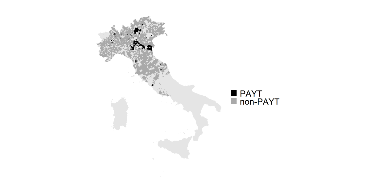
(a)

Figure 1: Map of PAYT and non-PAYT municipalities in the sample. White areas show the excluded South and Islands, municipalities with missing values, and those adopting PAYT before 2012.

This data allow for (counterfactual) predictions of policy effects for 26 million people (45% of the population) living in 3,380 municipalities without PAYT.

Variables come from a variety of sources. Waste generation and management costs are from the National Environmental Protection Agency (ISPRA). Municipal socio-economic attributes are from the National Institute of Statistics (ISTAT) and web scraping the online database of comuni-italiani.it. Political variables on, e.g., municipal elections and mayors’ characteristics are obtained from the Ministry of the Interior. Geographic variables measuring, e.g., the distance to waste treatment sites are geocoded using the software R and data of the European Pollution Release and Transfer Register (E-PRTR).

At the time of writing, there is no open-source database on PAYT prices in Italy. I acquired the list of PAYT municipalities from the National Environmental Protection Agency (ISPRA), the National Association of Italian Municipalities (ANCI), and from waste management companies. I collected a cross-section of price data directly from municipalities and waste companies, and indirectly from municipal balance sheets. Each municipality sets the same price over the three post-policy years analyzed in this study. Variables are described in Appendix B.

1.3 Summary statistics

Table LABEL:tab:nevertreated compares attributes of never-treated (non-PAYT) and treated (PAYT) units before policy. The main outcomes are yearly kilograms of per capita unsorted (UW), recycling waste (RW), and total (TW) which is the sum of the previous two. Municipal socio-economic characteristics such as average household size, income per capita, social deprivation index, commuting intensity, and migration flows are based on annual population data. Table LABEL:table:var_desc in Appendix presents a detailed description of all variables and units of measurement. The relevant groups of predictors are discussed in the next section.

Table 1: Summary statistics for never-treated vs. treated municipalities before policy. Observations equal 18,812 for never-treated (unbalanced panel) and 636 for treated before policy (balanced). Data includes 44 lag values of outcomes and costs for a total of 90 covariates.

		Never-treated		Treated (before)
Obs. 19,448		Mean	Sd	Mean	Sd
Outcomes:	Recycling Waste (RW) kg p.c.	233.9	82.84	296.8	89.9
	Unsorted Waste (UW) kg p.c.	223.5	120.5	216.0	115.1
	Total Waste (TW=RW+UW)	457.4	127.0	512.7	142.9
Costs € :	RW unit costs per kg	0.18	0.12	0.16	0.08
	UW unit costs per kg	0.28	0.19	0.29	0.16
	RW management costs p.c.	40.34	22.48	47.73	24.31
	UW management costs p.c.	53.83	34.26	50.01	23.88
Socio-economic	Population density	337.29	579.97	286.47	406.30
covariates:	Household size	2.31	0.34	2.50	0.72
	Income p.c. (x € 1,000)	13.86	2.29	14.22	1.97
	Net migration p.c.	0.003	0.01	0.02	0.64
	Population (x 1,000)	7.35	34.72	9.74	21.20
	Share of foreign population	0.08	0.04	0.10	0.04
	Share of male population	0.49	0.02	0.49	0.01
	Population growth	0.003	0.15	0.03	0.12
	Tourism p.c.	0.33	0.85	0.27	0.82
	Share of pop. aged $<5$	0.05	0.01	0.05	0.01
	Share of pop. aged $<14$	0.13	0.03	0.14	0.02
	Share of pop. aged $>65$	0.23	0.05	0.21	0.04
	Pop. share w. elementary deg.	0.31	0.05	0.31	0.04
	Pop. share w. college deg.	0.09	0.03	0.09	0.03
	Share of rented houses	0.09	0.03	0.09	0.02
	Housing density	2.30	0.27	2.23	0.25
	Share of single-parent families	0.10	0.02	0.10	0.01
	Share of students aged $>15$	0.06	0.01	0.06	0.01
	Share of commuters	0.26	0.06	0.25	0.05
	Social deprivation index	-1.50	1.58	-1.79	1.25
	Out of labor force/active pop.	0.63	0.06	0.62	0.05
	Unemployment rate	0.07	0.02	0.06	0.02
	Commuting intensity	0.44	0.13	4.52	12.80
Geographic	Km to PAYT city	50.00	63.23	33.75	37.97
covariates:	Km to hazardous waste site	13.80	15.40	9.37	9.15
	Km to incinerator	29.00	28.39	21.71	19.35
	Km to landfill	11.21	10.95	7.50	6.34
	Province or region capital (0/1)	0.01	0.12	0.04	0.19
	Province capital (0/1)	0.01	0.10	0.03	0.17
	Region capital (0/1)	0.003	0.06	0.005	0.07
	Medium urbanization (0/1)	0.38	0.49	0.51	0.50
	High urbanization (0/1)	0.20	0.40	0.16	0.37
	Low urbanization (0/1)	0.42	0.49	0.33	0.47
Political	Political participation	0.69	0.09	0.64	0.21
covariates:	Vote share big-tent party	0.23	0.07	0.23	0.05
	Vote share extreme left	0.07	0.10	0.06	0.02
	Vote share extreme right	0.13	0.08	0.12	0.06
	Local mayor (0/1)	0.76	0.42	0.86	0.35
	Centre-party mayor (0/1)	0.003	0.05	0.00	0.00
	Green-party mayor (0/1)	0.01	0.11	0.02	0.15
	Left-party mayor (0/1)	0.07	0.25	0.09	0.28
	Other-party mayor (0/1)	0.11	0.32	0.11	0.31
	Local-party mayor (0/1)	0.71	0.46	0.64	0.48
	Right-party mayor (0/1)	0.10	0.30	0.14	0.35
	Mayor’s age	52.04	10.47	50.80	10.18
	Mayor’s years of office	1.84	1.38	1.83	1.28

Municipalities generate relatively more RW than UW on average. Managing one unit of UW costs on average twice as much as RW. However, municipal unit costs are largely heterogeneous, and for some of these municipalities (40%) unit costs of RW are higher than those of UW. Table LABEL:tab:nevertreated also shows that average costs for UW are slightly higher in per capita terms. Per capita costs indicate that one individual on average spends about € 100 per year for waste services, and pays the most for unsorted waste. This implies that UW reductions that do not translate into RW increases will potentially drive cost savings for both households and municipalities. Previous studies point to education and income levels as key determinants of policy adoption and effectiveness (see, e.g., Gradus et al., 2019; Kinnaman, 2006). In my sample, PAYT is implemented in municipalities with on average slightly higher income and comparable education levels.

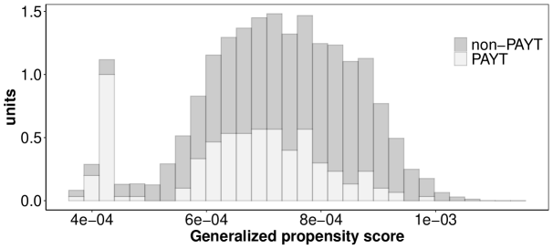
(a)

Figure 9: Common support condition for treated (PAYT) and never-treated (non-PAYT).

In order to obtain credible estimates of PAYT causal effects for each price level, all municipalities must have close comparisons in the opposite treatment group (PAYT/non-PAYT) for unbiased estimates of the causal effects without extrapolation (Imbens and Rubin, 2015). Overlap in the estimated (continuous) treatment propensities guarantees that a comparable unit can be found for each municipality. For a continuous treatment, the generalized propensity score (GPS) is the conditional probability of receiving a particular level of the treatment given the covariates (Imbens, 2000). Figure 9 in Appendix shows that PAYT units are fully in the support of non-PAYT units. Overlap statistics show that treated and control groups are similar in their GPS means, first and third quartiles. Moreover, the (normalized) difference in the estimated GPS amounts to less than one standard deviation (0.62), showing that the two groups are not apart. All municipalities satisfy the overlap assumption and can be included in the analysis.

Focusing on treated municipalities, Table 2 compares per capita waste amounts and municipal waste management costs before and after policy.

Table 2: Before-and-after comparison of waste outcomes and management costs of treated units. Observations equal 1,164 for 194 treated units observed over all years (balanced panel).

		Before		After
Obs. 1,164		Mean	Sd	Mean	Sd
Outcomes:	Recycling Waste (RW) kg p.c.	296.8	89.90	337.9	92.10
	Unsorted Waste (UW) kg p.c.	216.0	115.1	115.9	80.90
	Total Waste (TW=RW+UW)	512.7	142.9	453.8	127.2
Costs € :	RW management costs p.c.	47.73	24.31	54.29	20.20
	UW management costs p.c.	50.01	23.88	40.31	18.11
	RW unit costs per kg	0.16	0.08	0.17	0.07
	UW unit costs per kg	0.29	0.16	0.43	0.26

As expected, UW and TW decrease, and RW increases after PAYT. This leads to higher costs of RW and lower costs of UW per capita. Unit costs of UW increase after policy suggesting possible economies of scale. Yet, noticeably larger standard deviations relative to the mean indicate that average effects mask important heterogeneities across municipalities.

Table 3 reports price summary statistics by policy year, namely, for municipalities observed after one, two, and three years after policy adoption. Municipalities adopted PAYT starting from 2012 onward, so policy years range between 2012 and 2015. In addition, I have collected data for 2010 and 2011 to make sure to have at least two pre-policy years for all PAYT municipalities included in the sample. Prices range between 1 cent and 18 euro cents per liter of UW, for a total of 45 price levels. The average price is 8 cents, and the standard deviation is 0.05. Performing Wilcoxon and Kolmogorov-Smirnov tests (1945; 1971) shows that price distributions do not statistically differ across policy years.

Treatment	Year	Mean	Sd	Min	P50	P75	Max
PAYT price €  per liter	1 (obs. 194)	0.073	0.046	0.01	0.066	0.13	0.18
	2 (obs. 161)	0.080	0.046	0.01	0.079	0.13	0.18
	3 (obs. 125)	0.088	0.044	0.01	0.090	0.13	0.18

Table 3: Price summary statistics for PAYT municipalities by policy year.

Using prices and UW post-policy, I calculate household variable costs in each municipality. In the third policy year, households in high-price municipalities ($>$13 cents) pay on average € 176 per capita. In low-price municipalities ($<$3 cents), they pay on average € 21 per capita. The magnitude of this gap raises several questions. After partialling out confounding factors, do reactions in municipalities setting high versus low prices differ? What role do income effects play in driving these differences? More broadly, how do behaviors toward recycling and total waste adjust to a decrease in unsorted waste?

1.4 Determinants of waste generation and policy adoption

A large number of variables (confounders) can explain the decision to adopt PAYT as well as differences in waste generation across municipalities. I control for a large set of observables (deconfounders) that potentially affect household waste generation and policy adoption decisions at municipal level. Municipalities decide to implement PAYT because of possibly many individual or combined factors (Gradus et al., 2019): high levels of waste and/or waste management costs pre-policy, awareness of the waste pollution problem, citizens’ demand for higher-quality services, political variables, social norms, information effects, a developed recycling infrastructure and large administrative capacity. Further, as shown in Bueno and Valente (2019), leftover unobserved time-varying heterogeneity can be controlled for by including outcome lags. As a result, I include waste generation and policy adoption determinants for a total of 90 municipal attributes which can be grouped into five categories: socio-economic and geographic characteristics, political variables, pre-policy waste amounts and management costs.

Socio-economic characteristics.–This group of covariates proxies for heterogeneous household opportunity costs of time and space. Above all, the literature highlights income and education levels. The latter is measured by the population share with graduate degree or higher, and elementary degree or none. Income effects are indeterminate a priori (Callan and Thomas, 2006). Higher-income households may be less elastic due to, e.g., lower budget constraints and higher time opportunity costs. Both education and income may proxy for citizens’ demands for environmental quality (Dunlap et al., 2000). These variables, therefore, may drive both policy adoption and effects. Further, I control for municipal level demographics as, e.g., average house size and home ownership (based on the 2011 Italian national census), average household size and age (based on annual population data), and tourism intensity (in per capita values based on annual population data). Labor market attributes proxy for, e.g., time spent at home. I include the share of unemployed and out-of-the-labor force population, and indeces of labor market activity, commuting intensity, and social deprivation (based on annual population flows). Table LABEL:table:var_desc in Appendix presents a detailed description of all variables and units of measurement.

Geographic characteristics.–I control for the distance of each municipality to waste incinerators, landfills, and hazardous waste treatment facilities. Proximity to waste sites may induce, for instance, lower waste generation through households’ pollution awareness. In addition, distant waste sites may cause high transportation costs and, therefore, correlate with price adoption decisions. I further distinguished communities by urbanization levels, and regional or provincial seats. These variables proxy for differences in administrative capacity, recycling infrastructure, and PAYT system (Gradus et al., 2019).

Moreover, municipalities may adopt PAYT to mimic successful neighbors’ policies (Allers and Hoeben, 2010). In other words, vicinity to other PAYT municipalities may matter because of information dissemination. As a proxy, I control for the distance to the closest municipality that implemented PAYT in prior years.

Political variables.– Policymakers may adopt PAYT in response to citizens’ demand for, e.g., better service quality, lower waste charges, and fairer waste pricing (Dijkgraaf and Gradus, 2009; Batllevell and Hanf, 2008). Public engagement may correlate with waste behaviors as well as with policy acceptance and reactions to policy. To proxy for political participation, I include municipal level voter turnouts in the 2013 Italian general election. Political polarization and lack of social cohesion may also impact policy adoption and responses on waste generation. Protest votes and extreme ideology are proxied by vote shares for big-tent parties, and for extreme left- and right-wing parties.

Moreover, mayor characteristics can matter for policy adoption decisions and also for waste outcomes because they may shape waste-friendly behaviors. Newly elected, young mayors may be willing to invest in waste technology; citizens may elect green mayors putting PAYT in their agenda; locally born mayors of regional parties may promote pollution-saving behaviors, and may rely on large consensus and push reforms. To control for this, I add mayor’s age, term length, party, and place of birth.

Pre-policy waste generation.–Lagged waste generation may drive policy adoption as well as effect heterogeneity (Kinnaman, 2006). In fact, lagged waste outcomes reflect initial opportunity costs of household recycling and waste avoidance, and account for existing differences in the recycling infrastructure, e.g., at the curb. The waste generation history also contains information about unobservables such as motivation and experience in waste reduction, and pro-environmental attitudes (Bueno and Valente, 2019). Including lagged waste amounts, therefore, accounts for possible time-varying effects of fixed unobservables.

Pre-policy waste management costs.–Policy adoption decisions largely rely on municipal cost levels, both in per capita and per kg terms. If salient to the household, lagged per capita costs may also impact household waste generation. Cost variables include budgetary costs for waste collection (e.g., labor), disposal (e.g., machinery and land), transportation (e.g., trucks), treatment, and administrative services, net of recycling revenues from selling products and energy recovery.

2 Modeling Framework

I am interested in how a price on household unsorted waste disposal affects waste generation and costs at municipal level. Municipal costs are measured as the sum of waste management costs of unsorted and recycling waste. How do PAYT-induced changes in household waste generation affect municipal costs? This depends on the relative size of cost savings from unsorted waste reductions versus additional costs of increased recycling. Thus, empirically, it is key to understand the behavioral mechanism behind PAYT causal effects, namely, the extent to which unsorted waste reductions translate into more recycling and lower total waste.

To guide the interpretation of my empirical findings presented below, I construct a simple model of household behavior building on the seminal contribution of Kinnaman (2017). The model delivers two key empirical predictions. First, after PAYT introduction, households are predicted to increase recycling and reduce total waste. Second, household responses are heterogeneous depending on, in particular, income and waste generation habits.

2.1 Theoretical model

Consumption generates waste. A household generates unsorted waste $UW$ from consumption, and spends time and effort to recycle the amount $RW$. The opportunity cost of time is the hourly wage $w$, and the marginal cost of recycling is $\chi RW$ where $\chi$ is the amount of effort required for recycling. Proxies for $\chi$ are household demographics and other waste generation determinants described in Section 1.4. Households can work $H$ hours for a salary $wH$ and can spend part of this time $h_{RW}$ in sorting recyclable materials. Total waste $TW=RW+UW$ is a fraction $1/\alpha$ ($<$1) of the composite consumption good $c$, such that $TW=(1/\alpha)c$ or $c=\alpha TW$. Households pay a price $p_{c}$ for consumption and $p_{UW}$ for unsorted waste disposal. The price $p_{UW}$ is the PAYT price, if any, charged by the municipality for each unit of $UW$. The household utility-maximizing problem is:

$$U=U(c)\ \ \ \text{subject to}\ \ \ wH-wh_{RW}=p_{c}c+p_{UW}UW,$$ (1)

where $U(c)$ is utility from consumption ($U_{c}>0$, $U_{cc}<0$). Equation (1) states that households maximize utility from consumption and use their income $wH-wh_{RW}$ to pay for consumption and unsorted waste disposal. Substituting for $c=\alpha TW$ and assuming the recycling cost function $h_{RW}=h(RW)=\frac{\chi RW^{2}}{2}$ as in Kinnaman (2017) leads to the Lagrangian:

$$\mathcal{L}=U[\alpha(RW+UW)]+\lambda[wH-w(\frac{\chi RW^{2}}{2})-p_{c}\alpha(RW+UW)-p_{UW}UW],$$ (2)

where $\lambda$ is the marginal utility of income. Solving for the first-order conditions (reported in Appendix A.1) shows that $p_{UW}=w\chi RW$, namely, households choose the optimal amount of recycling when the marginal cost of recycling equals the marginal cost of unsorted waste disposal.

How does an exogenous increase in $p_{UW}$ due to PAYT adoption affect the optimal choice of $RW^{*}$ and $UW^{*}$? Using the first-order conditions, I derive three key comparative statics that will form the basis for my empirical analysis. The proofs are relegated to Appendix A.1.

Result 1.– After PAYT introduction, households reduce unsorted waste, an effect driven by an increase in recycling and a reduction in total waste:

$$\frac{\delta UW^{*}}{\delta p_{UW}}=-\frac{1}{w\chi}-\frac{UW^{*}}{\alpha U_{c}/\lambda^{*}}<0$$ (3)

$$\frac{\delta RW^{*}}{\delta p_{UW}}=\frac{1}{w\chi}>0.$$ (4)

This result shows that households decrease unsorted waste due to two effects. Equation (4) shows an increase in recycling (“substitution” effect). Equation (5) shows a reduction in total waste due to less consumption (“income” effect):

$$\frac{\delta TW^{*}}{\delta p_{UW}}=\frac{\delta RW^{*}}{\delta p_{UW}}+\frac{\delta UW^{*}}{\delta p_{UW}}={\frac{\delta RW^{*}}{\delta p_{UW}}}-{\frac{\delta RW^{*}}{\delta p_{UW}}}-\frac{UW^{*}}{\alpha U_{c}/\lambda^{*}}=-\frac{UW^{*}}{\alpha U_{c}/\lambda^{*}}<0.$$ (5)

Result 2.– The effects of PAYT are heterogeneous depending on, in particular, income and waste generation habits.

First, the increase in recycling is larger for households with lower costs of time and effort, namely, low-wage households (low $w$) and households who find recycling easier (low $\chi$). Second, the reduction in total waste is larger for high-waste households (high $UW^{*}$, low $\alpha$), and for households with higher marginal utility of income (high $\lambda^{*}$) and lower marginal utility of consumption (low $U_{c}$). Therefore, I expect that, especially, income and pre-policy levels of recycling and unsorted waste can be important predictors of PAYT effect heterogeneity.

Summing up, this simple model predicts that, after PAYT adoption, municipalities experience a reduction in unsorted waste, an increase recycling and a decrease in total waste. The heterogeneity in household responses, coupled with the large heterogeneity in municipal waste management costs (see Table LABEL:tab:nevertreated), make the sign and magnitude of PAYT effects on municipal costs ex-ante ambiguous and, thus, an empirical question.

2.2 Identification and empirical specification

I follow the potential outcome approach (Rubin, 1974). Let $(X_{it},Y_{it},P_{it})$ be the available data for municipality $i=1,...,n$ at time $t=2010,...,2015$, where $X_{it}\in\mathbb{R}^{d}$ is a vector of $d$ covariates, $Y_{it}$ is the waste outcome for either unsorted (UW), recycling (RW), or total waste (TW), and $P_{it}\in\mathcal{P}=[0;p_{max}]$ is the PAYT price (fee) or “treatment” variable in year $t$. Henceforth, I omit the true subscript $t$ for simplicity whenever possible. Note that prices range between zero (for all untreated years, namely, pre-treatment years for PAYT municipalities or any year for non-PAYT municipalities) and the maximum price set in treated years ($p_{max}$). For every unit $i$, there is a set of potential waste outcomes $Y_{i}(p)$, $p\in\mathcal{P}$, each being a random variable mapping a particular potential treatment, $p$, onto a potential outcome such that $Y_{i}=Y_{i}(p)$. This is also referred to as the unit level dose-response function. For any municipality defined by a vector of characteristics $X_{i}=x$, I wish to estimate the individual treatment effect of unit $i$, which is defined as $Y_{i}(p)-Y_{i}(0)$ and is, however, unobserved for any unit. Therefore, I will estimate the Conditional Average Treatment Effect (CATE) function and its derivative, the Conditional Average Price Effect (CAPE) function:

$$CATE=\Delta(x)={\mathbb{E}}\left[Y_{i}(p)-Y_{i}(0)|X_{i}=x\right]$$ (6)

$$CAPE=\delta(x)=\partialderivative{{\mathbb{E}}\left[Y_{i}(p)|X_{i}=x\right]}{p},$$ (7)

under the “canonical” assumptions of unconfoundedness and no spillovers (more precisely, the SUTVA or Stable Unit Treatment Value Assumption as in Rosenbaum and Rubin 1983; Imbens and Rubin 2015). I refer to Hirano and Imbens (2004) and Imai and van Dyk (2004) for a description of these assumptions. In essence, unconfoundedness requires to have enough controls - usually pre-treatment covariates and outcomes - so that, conditional on those controls, treatment assignment is as good as randomized. In the case of multivalued treatment, this assumption writes $Y_{i}(p)\mathchoice{\mathrel{\hbox to0.0pt{$\displaystyle\perp$\hss}\mkern 2.0mu{\displaystyle\perp}}}{\mathrel{\hbox to0.0pt{$\textstyle\perp$\hss}\mkern 2.0mu{\textstyle\perp}}}{\mathrel{\hbox to0.0pt{$\scriptstyle\perp$\hss}\mkern 2.0mu{\scriptstyle\perp}}}{\mathrel{\hbox to0.0pt{$\scriptscriptstyle\perp$\hss}\mkern 2.0mu{\scriptscriptstyle\perp}}}P_{i}|X_{i}$ $\forall p\in[0;p_{max}]$, i.e., requires conditional independence to hold for each value of the treatment. Imbens (2000) referred to this as weak unconfoundedness, since it does not require joint independence of all potential outcomes. While this assumption is not directly testable, I make it plausible by controlling for a large set of covariates and pre-policy outcomes. I further assess unconfoundedness in Section E.1.

SUTVA excludes the possibility of interference between units and, given the observed covariates, allows to consider the potential outcomes of one unit to be independent of another unit’s treatment status. To make this assumption more reliable, I control for information effects across treated units, and I assess robustness to spillovers in untreated units (see Sections 1.4 and E.1).

In order to fulfill unconfoundedness in the case of non-random price adoption, one needs to control for the sources of self-selection, i.e., capture the effect of $X_{i}$ on $P_{i}$. Consider the partially linear waste outcome model:

$$Y_{i}={\mathbb{E}}\left[Y_{i}(0)|X_{i}\right]+P_{i}\delta(X_{i})+\epsilon_{i}(P_{i}).$$ (8)

Under unconfoudedness, ${\mathbb{E}}\left[\epsilon_{i}(P_{i})|X_{i},P_{i}\right]=0$; further, ${\mathbb{E}}\left[Y_{i}(0)|X_{i}\right]$ represents the possibly non-linear direct effect of covariates on untreated outcomes. Note that $X_{i}$ is of potentially very high dimension. Let ${\mathbb{E}}\left[Y_{i}|X_{i}\right]$ be the conditional outcome mean, and ${\mathbb{E}}\left[P_{i}|X_{i}\right]$ the conditional price mean (or “propensity score”), respectively. By means of algebraic transformations (see proofs in Appendix A.2), model (8) can be rewritten as:

$$Y_{i}-{\mathbb{E}}\left[Y_{i}|X_{i}\right]=(P_{i}-{\mathbb{E}}\left[P_{i}|X_{i}\right])\delta(X_{i})+\epsilon_{i}(P_{i}),$$ (9)

where $\delta(X_{i})$ identifies the CAPE as the effect of the leftover price variation $P_{i}-{\mathbb{E}}\left[P_{i}|X_{i}\right]$ on the leftover outcome variation $Y_{i}-{\mathbb{E}}\left[Y_{i}|X_{i}\right]$ not explained by the observed covariates. The standard partially linear model considers solely the case of constant treatment effects (Robinson, 1988). Yet, Nie and Wager (2021) study identification of model (9) for flexible heterogeneous treatment effect estimation via machine learning approaches. In particular, we can estimate $\delta(x)$ in two steps: First, we separately estimate the nuisance components ${\mathbb{E}}\left[Y_{i}|X_{i}=x\right]$ and ${\mathbb{E}}\left[P_{i}|X_{i}=x\right]$. Second, we plug in their fitted values to obtain $\hat{\delta}(x)$ by regressing residualized outcomes on residualized prices. In this step, we do not consider all residuals as equally important, and we estimate a local version of model (9) that gives more weight to those residuals in the neighborhood of $x$ (see the next subsection for details).

Residual-on-residual regression methods, also known as R(esidualized)-learning in high-dimensional settings, make the parameter estimate insensitive to small errors in the nuisance components, thus improving its robustness. The final estimator combining predictions from two models is robust to possible misspecifications in either the outcome model or the propensity score model (Nie and Wager, 2021). Note that, as an alternative approach, one could directly estimate model (8) by including the high-dimensional covariate set. However, regularization of ${\mathbb{E}}\left[Y_{i}(0)|X_{i}\right]$ would cause an especially large bias when covariates are correlated with prices (Athey et al., 2017; Chernozhukov et al., 2017). Conversely, residualization removes the correlation of covariates with both prices and outcomes, rendering the estimator robust to the parametric form in which covariates are included. In particular, as long as either the estimator for either propensity scores or conditional outcome expectation is consistent, the resulting estimator for the treatment effect is consistent (Nie and Wager, 2021).

2.3 Random forests for heterogeneous policy effects

I now discuss how to estimate equation (9) for each municipality $i$ described by the covariate vector $X_{i}=x$. First, I estimate ${\mathbb{E}}\left[P_{i}|X_{i}\right]$ for $X_{i}=x$, which defines the generalized propensity score $s(x)\coloneqq{\mathbb{E}}\left[P_{i}|X_{i}=x\right]$. Second, I estimate ${\mathbb{E}}\left[Y_{i}|X_{i}\right]$ for $X_{i}=x$, which defines the expected outcome marginalizing over treatment $y(x)\coloneqq{\mathbb{E}}\left[Y_{i}|X_{i}=x\right]$. Third, I use $s(x)$ and $y(x)$ to estimate $\delta(X_{i})$ for $X_{i}=x$, which defines the CAPE $\delta(x)$. To explicitly account for heterogeneity in the parameter estimation procedure, I propose to use the Random Forest (RF) estimator developed in Athey et al. (2019). This method generalizes the original algorithm of Breiman (2001) by adapting to the problem of heterogeneous treatment effect estimation.

RFs present several advantages compared to other methods. First, standard $k$-nearest neighbor/kernel matching methods are bound to fail, as the concept of neighbor vanishes in high-dimensions (Abadie and Imbens, 2016; Giraud, 2015). Conversely, RFs are adaptive (data-driven) matching estimators that can estimate neighbors in a high-dimensional space while avoiding overfitting through the use of both training and estimation samples. Second, RFs are nonparametric techniques relying on recursive, data-driven sample splits to capture possibly complex non-linear interactions between covariates and treatment effects without assumptions regarding the data distribution. This reduces the risk of model misspecification and limits researcher discretion when selecting the relevant dimensions of heterogeneity. Third, and most importantly, RFs are consistent estimators of the full mapping of CAPE; in other words, they allow to construct a policy targeting function mapping observed covariates onto unit level causal effects.

Breiman’s RF is understood as an ensemble method averaging predictions made by individual trees. Yet, as shown in Athey et al. (2019), we can equivalently think of RF as an adaptive kernel method. For instance, we can re-write the forest prediction as $\hat{y}(x)=\sum_{i=1}^{n}w_{i}(x)Y_{i}$ where $w_{i}(x)$ is a data-adaptive kernel that measures how often the $i^{th}$ training unit falls into the same leaf as $x$. How does the RF determine the weighted set of neighbors for any test point $x$?

Step 1: Random subsampling. Grow a set of $B$ trees and, for each tree, $b=1,\dots,B$, draw a random subsample of training data $s_{b}^{tr}\subseteq\{1,\dots,n\}$.

Step 2: Recursive partitioning. Estimate a tree via recursive partitioning on $s_{b}^{tr}$ and a random subset of covariates. During each partitioning step, split the training sample according to any cutpoint of each covariate, and obtain two new partitions. In each partition, run model (9) to estimate $\hat{\delta}(x)$ and its variance across partitions. Repeat this step using every covariate and select the one that leads to the largest CAPE heterogeneity (variance). Split the data into two subgroups based on the optimal cutpoint in the selected covariate. Thus, the selected predictor becomes a partitioning variable. Continue partitioning $s_{b}^{tr}$ a number of times until the splitting process terminates after a particular stopping criterion is reached. The resulting tree is a sequence of binary regions partitioning the covariate space and grouping observations in the bottom regions called leaves $L_{b}$.

Step 3: Prediction. Define $L_{b}(x)$ as the set of training observations falling in the same neighborhood (leaf) as $x$. Each tree gives equal (positive) weight to the observations in the same leaf as the test point $x$, and zero weight to all the other observations. Then, the forest averages all these tree-based weightings, measuring how often each training example $i$ falls into the same leaf as $x$. This measure is given by the forest weights $w_{i}(x)$:

$$w_{ib}(x)=\frac{\mathbbm{1}({X_{i}\in L_{b}(x)})}{|L_{b}(x)|}\ \ ,\ \ w_{i}(x)=\frac{1}{B}\sum_{b=1}^{B}w_{ib}(x),$$ (10)

where $\sum_{i=1}^{n}w_{i}(x)=1$. For more details, see Athey et al. (2019).

This kernel-based perspective of RFs allows to cast this method as an adaptive locally weighted estimator that first uses a forest to calculate a weighted set of neighbors for each test point $x$, and then solves a weighted version of the residual-on-residual regression (9). The resulting CAPE estimator writes:

$$\hat{\delta}(x)=\frac{\sum_{i=1}^{n}w_{i}(x)(Y_{i}-\hat{y}^{-i}(X_{i}))(P_{i}-\hat{s}^{-i}(X_{i}))}{\sum_{i=1}^{n}w_{i}(x)(P_{i}-\hat{s}^{-i}(X_{i}))^{2}},$$ (11)

where $\hat{s}^{-i}(X_{i})$ are out-of-sample predictions of the propensity scores $s(x)$. Equation (11) characterizes the CAPE as a weighted residual-on-residual regression estimator with forest weights $w(x)$ defining the nearest neighbors of $x$ produced by different trees. This distinguishes the CAPE from the APE (Average Price Effect) estimator which is the unweighted version of (11). Variance of $\hat{\delta}(x)$ is estimated by evaluating the estimator on bootstrapped half-samples of the training data, also called bootstrap of little bags (Athey et al., 2019; Sexton and Laake, 2009).

3 Main Results

I estimate separate random forests for each outcome (unsorted, recycling, total waste per capita) and policy year. A tree is built with data for the same calendar year to account for common shocks to all units. In order to account for the staggered nature of the intervention, treated units in a given policy year are matched with never-treated units only. In other terms, late adopters are not included in the control group of early adopters. This is important especially since lagged outcomes are included among the covariates.

I have explored from 500 to 10,000 trees in the RF, and treatment effect estimates become stable after 1,000 trees, thus, results are obtained using this value. All trees are grown with cross-validated values for the number of randomly subsampled covariates, minimum leaf size, and penalty for imbalanced splits, namely, splits in which the size of parent and child node are very different are penalized. To overcome the issue that the treatment group is substantially smaller than the control group, each node is required to include a minimum number of both treated and control units, i.e., enough information about both factual and counterfactual to estimate the treatment effect reliably. For this reason, a penalization is imposed also to nodes including an unbalanced number of treated and control units. Following Athey et al. (2019), values for such parameters are obtained via cross-validation.

In order to credibly estimate policy causal effects, the common support condition for treated and untreated units needs to hold. Figure 9 in Appendix C provides evidence of such support.

3.1 Policy effects on waste demands

I begin my empirical analysis by estimating the CAPE function in equation (11), namely, I estimate municipal level causal effects of prices on demands for unsorted, recycling, and total waste per capita (UW, RW, TW, respectively). In this section, I focus the attention on causal effects in the third policy year in order to have a closer estimate to the long-term effects of PAYT. I run separate random forests for each waste outcome: UW, RW, and TW (for robustness). Figure 2 presents the CAPE distribution for all municipalities in the sample. Price effects are estimated as price semi-elasticities of waste demands. All estimates are statistically different from zero (p-values $<$ 0.01). The hypothesis of effect homogeneity is rejected for all outcomes and policy years.

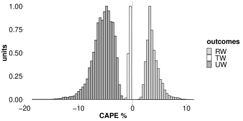
(a)

Figure 2: Unit level estimates of price semi-elasticities (CAPE) of waste demands. CAPE are measured as percent changes of waste amounts for a one cent price increase.

The estimated price effects on waste demands for UW and RW are large in magnitude. I use the estimated CAPE to compute factual and counterfactual waste amounts, and the percent (causal) change in waste relative to the counterfactual. I find that prices cause an annual UW decline of 50% on average. This reduction is mainly driven by an average RW increase of 32% and, to a lesser extent, by an average TW reduction of 5%. The large substitution effect of UW with RW caused by the policy, therefore, represents a strong change in waste behaviors.

3.2 Sources of causal effect heterogeneity

Using the CAPE function defined in equation (11) and estimated in the previous section, I proceed with the analysis of the sources of effect heterogeneity. In order to summarize the CAPE function, I linearly project the CAPE estimates onto price levels, a set of municipal characteristics, and their interactions. This corresponds to fitting the linear model:

$$\beta=\operatornamewithlimits{argmin}_{\beta}\{{\mathbb{E}}\left[(CAPE-X_{sub}\beta)^{2}\right]\}$$ (12)

where $CAPE$ are point estimates of the price causal effects (as presented in Figure 2), and $X_{sub}$ are explanatory variables including price levels, a subset of municipal characteristics, and their interactions. The literature on waste prices is especially interested in learning the elasticity of demand as a function of a few variables such as income or education. Thereby, the set of features includes relevant regressors capturing household opportunity costs of waste disposal: income, education, and pre-policy waste levels. Figure 3 plots fitted semi-elasticities (CAPE) across prices, ceteris paribus. Pointwise estimates are obtained by fitting a smooth regression line. Shaded regions are the 95% confidence intervals.

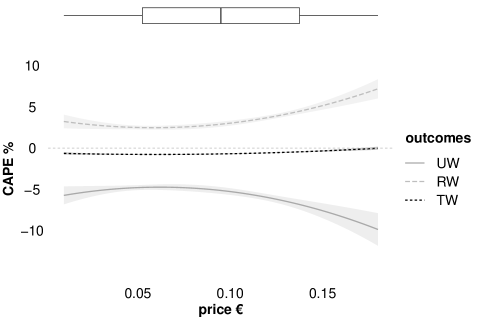
(a)

Figure 3: Fitted price semi-elasticities (CAPE) of waste demands at each price level.

Price elasticities of waste demands in high and low price regions differ. I use the median value of 9 cents to define these regions, indicated by the vertical line in the boxplot above the image. While at high prices elasticities are increasing, elasticities are rather constant at low prices. All other things equal, a one cent price increase reduces unsorted waste by 5 to 10% (vs. 4.7-5.7% at low prices), increases recycling by 2 to 6% (2.5-3.2%) and reduces total waste by 0.1 to 0.7% (0.6-0.8%) compared to a counterfactual zero-price (no PAYT) scenario. Further, demand responses at high prices shed new light on the mechanism behind UW reductions: increasing UW reductions reveal a negative correlation between TW and RW reactions, suggesting that waste reduction and recycling are substitute behaviors. Thus, higher prices do not cause further total waste reductions, instead they simply reallocate waste to the recycling pile.

Having established effect heterogeneity across prices, I analyze possible income effects. Figure 4 plots fitted semi-elasticities by income level, ceteris paribus.

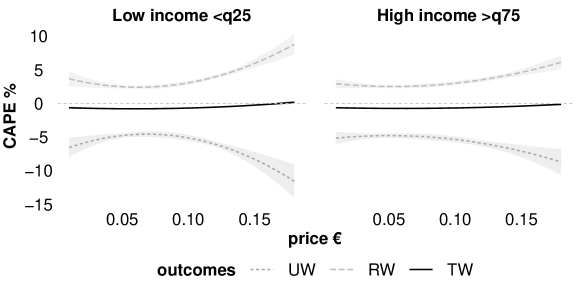
(a)

Figure 4: Fitted price semi-elasticities (CAPE) of waste demands by income levels. Thresholds q25 and q75 indicate first (€ 13k) and third (€ 16k) quartiles of annual income per capita.

Income differences across municipalities significantly explain price effect heterogeneity at high prices: Low-income municipalities are on average one percent point more elastic than high-income municipalities. This result is new to the literature as previous studies typically consider the effects of low prices. Differently, income effects are not statistically significant at low prices. This may be explained by the low monetary benefits of reducing UW at low prices: households reduce UW by 13.6% in the first price quartile (3 cents) and save less than one euro.

Additionally, price effects at high prices are heterogeneous also in recycling habits before policy, as predicted by Kinnaman (2006). In particular, high prices are effective in increasing recycling levels in low-recycling municipalities which have large margin to improve on this behavior.

Finally, looking at heterogeneity across education levels, I estimate no significant effects, suggesting that education plays, if any, a relatively minor role.

3.3 Comparison with the literature

Typically, the literature estimating demand responses of waste prices relies on the assumption that the mean price and waste quantity are on one point along the linear demand curve, and finds low average price elasticities (see, e.g., Kinnaman, 2006; Fullerton and Kinnaman, 2000). However, prior work analyzes waste programs with low adopted prices. The average point-price elasticity of unsorted waste demand across 72 studies amounts to -0.34 (Bel and Gradus, 2016). For comparison, I compute the point-price elasticity at mean price and quantity in the first and fourth quartile of the price distribution. I find a value of -0.26 in the lowest quartile, and a value of -2.2 in the highest quartile. In line with the literature, this study consistently estimates low price elasticities of waste demands when prices are low. Additionally, I show that waste demands are significantly more elastic at high prices.

3.4 Policy effects on municipal costs

Heterogeneity of policy effects on municipal budgets is driven by both demand and cost effects. For each municipality $i=1,...,n$ with attributes $X_{i}=x$, I define the policy Effects on Municipal Costs ${EMC}^{P>0}(x)$ in per capita euros as waste management cost savings caused by PAYT ($P>0$):

$${EMC}^{P>0}(x)=-\Bigg{[}{CATE}{{}_{UW}}PC_{UW}^{P>0}(x)+{CATE}{{}_{RW}}PC_{RW}^{P>0}(x)\Bigg{]},$$ (13)

where ${CATE}=p\hat{\delta}(x)$ (in kg per capita) and $\hat{\delta}(x)$ are statistically significant CAPE point estimates for each municipality and waste type. Further, $PC^{P>0}(x)$ are municipal (private) unit costs of unsorted or recycling waste management under PAYT (in € /kg). $PC^{P>0}(x)$ are observed for treated units (under treatment) but unobserved for untreated units. In this section, I estimate whether PAYT caused significant changes in unit costs of treated units using RF. In the next section, I use the estimated RF function to predict unit costs for untreated units under PAYT (see Section 3.5 for more details).

In my sample, unit costs of unsorted waste are higher than those of recycling for most municipalities. This implies that unsorted waste reductions that do not translate into an increase in recycling are the driving source of municipal cost savings. In other words, I expect demand responses on total waste to matter for effects on municipal budgets.

I start by documenting that demand effects (CATE) on UW and TW are lowest in the first policy year. This is consistent with economic theory showing that elasticities are typically lower in the short-run because fewer alternatives are available (Usui, 2009). UW reductions are largely driven by increased recycling and, to a smaller extent, by total waste reductions. In particular, behavior changes toward total waste are relatively smaller and slower. This is consistent with behavioral economic predictions by e.g. Cecere et al. (2014) who argue that changes in consumption habits and subsequent total waste reductions require more effort and learning than recycling.

Figure 5 plots the distribution of statistically significant demand effects on TW by policy year.

(a)

Figure 5: Unit level estimates of causal effects (CATE) on total waste demands in the second and third policy year (p-values $<$ 0.05). The y-axis refers to the number of treated municipalities.

In year 1, there are no statistically significant effects on total waste. In year 2, I observe significant reductions for about 30% of municipalities, and significant reductions for all municipalities in year 3.

Next, I flexibly estimate policy causal effects on unit management costs for UW and RW via random forests. I find that PAYT leaves unit costs of waste mostly unaffected. Finally, I compute policy effects on municipal costs by combining CATE with unit costs of waste management. Table 4 shows municipal cost effects (€  p.c.) by policy year.

	Year	Mean	Sd	EMC$>$0
EMC €  p.c.	1	0.13	10.16	36%
	2	3.14	7.10	89%
	3	20.17	16.28	all

Table 4: Summary statistics for policy Effects on Municipal Costs (EMC) for each PAYT municipality. EMC$>0$ indicate cost savings per capita (p.c.) by policy year.

Policy effects on municipal costs are mostly positive. However, waste prices raise municipal costs in a fraction of municipalities where the reduction of unsorted waste is largely driven by an increase in recycling, and management costs of recycling are high compared to those of unsorted waste. In year 3, PAYT generates cost savings in all municipalities. Average savings are € 20 per capita, which is about one fifth of what municipalities spend for waste management per person on average. As management unit costs are largely unaffected, savings come from UW reductions that do not translate into higher RW. In other words, municipal cost savings are largely driven by total waste reductions.

As higher prices promote increased recycling rather than waste avoidance, the largest cost savings occur in municipalities setting low prices after three years of adoption. Figure 6 shows effects on municipal costs at high vs. low prices (above vs. below the median) in the third policy year, when total waste reductions are highest.

(a)

Figure 6: Policy Effects on Municipal Costs (EMC$>$0 indicate cost savings) at high vs. low waste prices (above vs. below the median) after three years of adoption.

This implies that (i) higher prices may be less desirable from a municipal cost perspective as they do not cause further total waste reductions, instead they rather reallocate waste to the recycling pile, and (ii) targeting total waste reductions in high-price municipalities could increase savings substantially.

The final implication of this paper may help local governments to overcome their initial concerns regarding the implementation of PAYT policies. This paper provides evidence that short-term costs may indeed increase due to higher recycling, but these costs are outrun by the long-term savings due to total waste reductions.

3.5 Policy simulations for municipalities without PAYT

I estimate causal effects on waste demands and municipal costs if all municipalities in the sample were to implement PAYT. The estimation proceeds in four steps.

Step 1: Predict counterfactual prices. To each non-PAYT municipality, assign the price of the PAYT municipality with the closest predicted propensity score.

Step 2: Predict counterfactual ${CAPE}$. Predict price semi-elasticities for non-PAYT municipalities using the RF function mapping $X$ onto causal changes in waste amounts previously estimated for PAYT municipalities.

Step 3: Predict counterfactual ${CATE}$. Predict price effects (in kg) for non-PAYT municipalities multiplying statistically significant CAPE point estimates by the predicted PAYT price.

Step 4: Predict counterfactual ${PC}^{P>0}$. Predict municipal private unit costs for non-PAYT municipalities using the RF function mapping $X$ onto causal changes in unit costs previously estimated for PAYT municipalities. For each non-PAYT municipality, assess whether PAYT would affect unit costs significantly. If this is the case, replace the observed $PC^{P>0}$ in the absence of PAYT with its predicted counterpart under PAYT.

Figure 7 plots the predicted price semi-elasticities of RW and TW demands after three years of adoption. Color differences in the same area indicate that higher recycling is associated to smaller reductions in total waste and vice versa.

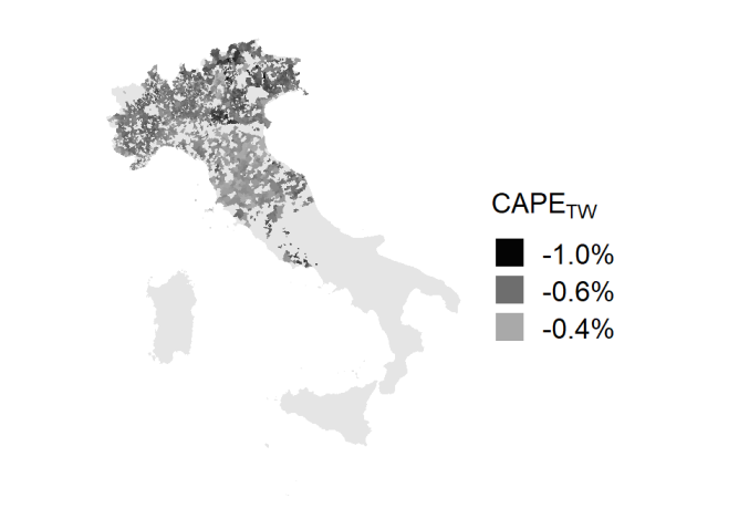
(a)

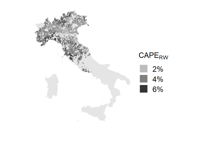
(b)

Figure 7: Predicted semi-elasticities (CAPE) on total waste and recycling demands for all municipalities three years after policy.

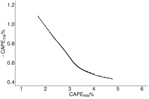
(a)

Figure 13: CAPE (semi-elasticities) for recycling ($x$-axis) plotted against CAPE for total waste reductions ($y$-axis). A smooth line is fitted through percentile values.

In particular, I estimate that a one percent point increase in $CAPE_{RW}$ decreases $CAPE_{TW}$ in absolute terms by on average 0.1 percent points (see Figure 13 in Appendix). Importantly, the elasticity of substitution between the effects on recycling and total waste does not lead to rebound effects (i.e., higher total waste).

Despite substitutabilities between waste reduction and recycling behaviors, policy simulations show that most municipalities would benefit from PAYT adoption. Table 5 shows predicted policy effects on municipal costs by policy year if all municipalities were to implement PAYT (distributions are plotted in Figure 14 in Appendix D.3).

	Year	Mean	Sd	EMC$>$0
EMC €  p.c.	1	1.45	10.90	50%
	2	3.95	9.33	73%
	3	23.85	18.33	99.8%

Table 5: Summary statistics for predicted policy Effects on Municipal Costs (EMC) for all observed municipalities. EMC$>0$ indicate cost savings per capita (p.c.) by policy year.

Compared to a counterfactual zero-price (no PAYT) scenario, UW reductions lead to a 24% decrease in municipal costs of waste management on average over the policy years. At the same time, increased RW raises municipal costs by on average 21%. In year 3, average per capita total cost savings amount to € 24, however, there is large variation. Figure 8 maps this variation: despite effect heterogeneity, waste prices cause cost savings for most municipalities.

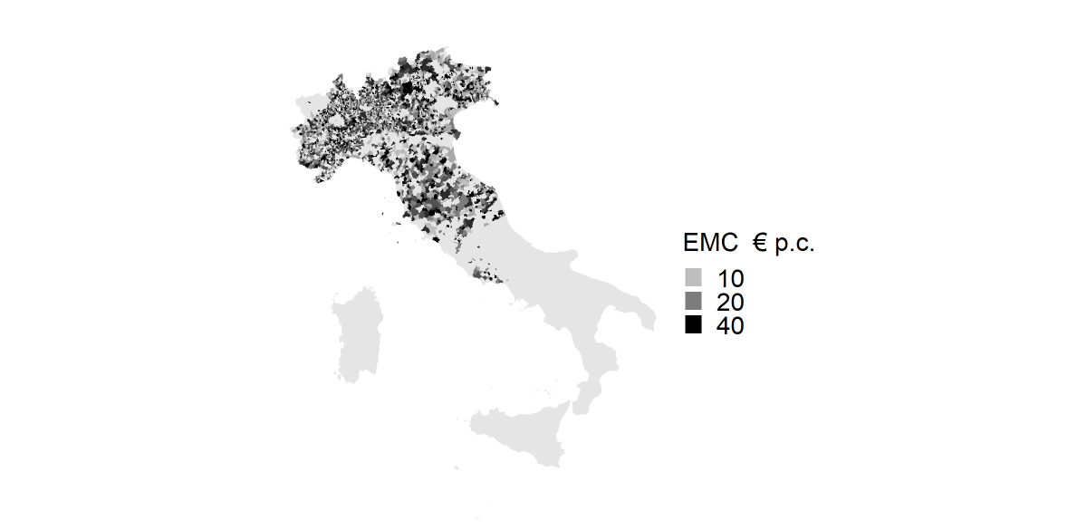
(a)

Figure 8: Distribution of predicted Effects on Municipal Costs (EMC) in the third policy year in €  per capita.

3.6 Robustness and sensitivity

I perform additional analyses to check whether my results are robust against the presence of unaccounted-for heterogeneity. In line previous findings (see Bel and Gradus, 2016, for a review), I find that my estimates are robust to confounding from adoption of heterogeneous PAYT systems (weight versus volume). Moreover, I find that waste tourism or, more generally, spillover effects are not relevant on any significant scale. See Appendix E.1 for more details.

Finally, I contrast my average estimates to the binary treatment case, two-way (event-study-like) fixed effects estimation (with/without re-weighting á la De Chaisemartin and D’Haultfœuille 2020), and R-learning LASSO regression. Results highlight the importance to account for continuous rather than binary treatment, the bias of the fixed effects estimator due to non-parallel trends pre-policy, and robustness to the specific choice of R-learning estimator. Full results are discussed in Appendix E.2.

4 Conclusions

This paper models and estimates causal effects of waste prices (PAYT) on recycling, unsorted, and total waste amounts by explicitly accounting for heterogeneity with machine learning methods. I analyze unique data with large variation in prices and a high-dimensional set of municipal characteristics. I estimate municipal level price elasticities using a random forest and R-learning estimator robust to confounding that affects outcomes and prices. By mapping municipal attributes onto causal effects, I predict heterogeneous policy effects for all municipalities in the sample, treated or not. The analysis of policy effects on municipal costs is motivated by a theoretical model that predicts heterogeneous waste behaviors in response to PAYT. Such heterogeneity in waste demands, coupled with the large heterogeneity in municipal waste management costs, make the sign and magnitude of PAYT effects on municipal costs ex-ante ambiguous and, thus, an empirical question.

Disentangling effect heterogeneity in prices from other sources, I find that waste demands are nonlinear. Low prices make waste demands similarly elastic, and trigger large unsorted waste reductions, increase recycling, and decrease total waste. High prices make waste demands increasingly elastic, and induce recycling rather than total waste reductions. On average, policy causal effects amount up to -50% on unsorted waste, 32% on recycling, and -5% on total waste. Income effects and waste habits pre-policy significantly explain price effect heterogeneity at high prices. I find that lower-income municipalities are more price elastic. Despite large effect heterogeneity, the policy reduces municipal costs in all municipalities after three years of adoption, especially where total waste reductions are large. This implies that higher prices may be less desirable from a municipal cost perspective as they do not cause further total waste reductions, instead they rather reallocate waste to the recycling pile. This study shows that price levels matter for waste behavior and municipal costs of waste management. Estimating heterogeneous responses on unsorted waste, and especially on recycling and total waste is crucial to assess overall policy effects on municipal costs. Reductions of total waste may not be immediate, and municipal costs may increase in the short-run. One upshot of this paper is that low prices can have a significant impact on waste behavior and municipal costs. Analyzing the long-term effects of PAYT policies presents an exciting research opportunity that I hope to tackle in future work.

Online Appendix

Appendix A Proofs

A.1 The theoretical model

Consider the Lagrangian (2). The first-order conditions for the choice variables $UW,RW$ are:

$$\alpha U_{c}/\lambda=p_{c}\alpha+p_{UW}$$ (14)

$$\alpha U_{c}/\lambda=p_{c}\alpha+w\chi RW$$ (15)

$$wH-w(\frac{\chi RW^{2}}{2})-p_{c}\alpha(RW+UW)-p_{UW}UW=0.$$ (16)

Solving (14) and (15) results in $p_{UW}=w\chi RW$ which says that households choose the optimal amount of recycling when the marginal cost of recycling equals the marginal cost of unsorted waste generation. The utility-maximizing solution for the choice of recycling is:

$$RW^{*}=\frac{p_{UW}}{w\chi}.$$ (17)

Differentiating this equation with respect to $p_{UW}$ leads to the comparative static (4): $\frac{\delta RW^{*}}{\delta p_{UW}}=\frac{1}{w\chi}>0$.

The utility-maximizing solution for the choice of unsorted waste is obtained by substituting (17) in (16):

$$wH-\frac{p_{UW}^{2}}{2w\chi}-p_{c}\alpha(\frac{p_{UW}}{w\chi}+UW^{*})-p_{UW}UW^{*}=0$$ (18)

Rearranging this equation in terms of $UW^{*}$ leads to:

$$UW^{*}(p_{c}\alpha+p_{UW})=wH-p_{c}\alpha\frac{p_{UW}}{w\chi}-\frac{p_{UW}^{2}}{2w\chi}.$$ (19)

Differentiating (19) with respect to $p_{UW}$ (using the quotient rule) gives:

$$\frac{\delta UW^{*}}{\delta p_{UW}}=\frac{-\frac{(p_{c}\alpha+p_{UW})}{w\chi}(p_{c}\alpha+p_{UW})-UW^{*}(p_{c}\alpha+p_{UW})}{(p_{c}\alpha+p_{UW})^{2}}.$$ (20)

After simplifying this last expression and using (14) to substitute for $(p_{c}\alpha+p_{UW})=\alpha U_{c}/\lambda^{*}$, we obtain the comparative static (3): $\frac{\delta UW^{*}}{\delta p_{UW}}=-\frac{1}{w\chi}-\frac{UW^{*}}{\alpha U_{c}/\lambda}<0$.

A.2 The econometric model

Consider the partially linear waste outcome model (8). Let us take the conditional expectation with respect to $X_{i}$ on both sides, change signs, and add $Y_{i}$ to both sides. We obtain:

$$\underbrace{Y_{i}}_{added}-{\mathbb{E}}\left[Y_{i}|X_{i}\right]=\underbrace{Y_{i}}_{added}-{\mathbb{E}}\left[Y_{i}(0)|X_{i}\right]-{\mathbb{E}}\left[P_{i}|X_{i}\right]\delta(X_{i})-{\mathbb{E}}\left[\epsilon_{i}(P_{i})|X_{i}\right],$$ (21)

where ${\mathbb{E}}\left[\epsilon_{i}(P_{i})|X_{i}\right]=0$. Substituting $Y_{i}$ on the right-hand side for the corresponding expression (8) gives:

$$Y_{i}-{\mathbb{E}}\left[Y_{i}|X_{i}\right]=\underbrace{{{\mathbb{E}}\left[Y_{i}(0)|X_{i}\right]}+P_{i}\delta(X_{i})+\epsilon_{i}(P_{i})}_{Y_{i}}{-{\mathbb{E}}\left[Y_{i}(0)|X_{i}\right]}-{\mathbb{E}}\left[P_{i}|X_{i}\right]\delta(X_{i}).$$ (22)

After simplifying and rearranging this last expression we get equation (9), namely, $Y_{i}-{\mathbb{E}}\left[Y_{i}|X_{i}\right]=(P_{i}-{\mathbb{E}}\left[P_{i}|X_{i}\right])\delta(X_{i})+\epsilon_{i}(P_{i})$.

Appendix B Descriptive statistics

Table 6: Variables’ description. Census indicates 2011 values (ISTAT, 2011).

	Variables’ description
PAYT price	Treatment: unit price on unsorted waste in €  per liter
Recycling Waste (RW) kg p.c.	Recycling waste per capita (kg)
Unsorted Waste (UW) kg p.c.	Unsorted waste per capita (kg)
Total Waste (TW=UW+RW)	Total waste per capita (kg)
UW management costs p.c	Per capita costs of UW management (€ )
RW management costs p.c	Per capita costs of RW management less RW revenues (€ )
UW unit costs per kg	Unit costs of UW management (€  per kg)
RW unit costs per kg	Unit costs of RW management less RW revenues (€  per kg)
Km to PAYT city	Distance to closest municipality with PAYT in t-1 (km)
Km to hazardous waste site	Distance to closest hazardous waste treatment facility (km)
Km to incinerator	Distance to closest waste incinerator (km)
Km to landfill	Distance to closest waste landfill (km)
Population density	Population density (inhabitants per km2)
Household size	Average household size (n. household members)
Income p.c.	Income per capita (x € 1,000)
Net migration p.c.	Net migrant flow per capita
Population	Population (x 1,000 inhabitants)
Share of foreign population	Share of foreign population
Share of male population	Share of male population
Population growth	Population growth
Tourism	Capacity of tourist accommodation per capita (x 1,000)
Share of population aged $<5$	Share of population aged less than 5 years old (census)
Share of population aged $<14$	Share of population aged less than 14 years old (census)
Share of population aged $>65$	Share of population aged more than 65 years old (census)
Pop. share w. elementary deg.	Share of pop. with elementary degree or lower (census)
Pop. share w. college deg.	Share of population with college degree (census)
Share of rented houses	Share of rented houses (census)
Housing density	Housing density (inhabitants per 100m2, census)
Share of single-parent families	Share of single-parent families (census)
Share of students aged $>15$	Share of student population older than 15 years old (census)
Share of commuters	Share of commuters (census)
Social deprivation index	Social deprivation index (-/+ deprived, census)
Out of labor force/active pop.	Out of labor force pop./pop. aged 15-64 years old (census)
Unemployment rate	Unemployment rate (census)
Commuting intensity	Commuting index (0-100, IIRFL) between cities (census)
Political participation	Voter turnout in the 2013 Italian general election (IGR13)
Vote share big-tent party	Vote shares for big-tent parties in the IGR13
Vote share extreme left	Vote shares for extreme left-wing parties in the IGR13
Vote share extreme right	Vote shares for extreme right-wing parties in the IGR13
Local mayor (0/1)	Mayor born in the municipal province (dummy)
Centre-party mayor (0/1)	Centre-party mayor (dummy)
Green-party mayor (0/1)	Green-party mayor (dummy)
Left-party mayor (0/1)	Left-wing mayor (dummy)
Other-party mayor (0/1)	Mayor of other party (dummy)
Local-party mayor (0/1)	Mayor of local party (dummy)
Right-party mayor (0/1)	Right-wing mayor (dummy)
Mayor’s age	Mayor’s age
Mayor’s years of office	Mayor’s term of office (years)
Province or region capital (0/1)	Either province or region capital (dummy)
Province capital (0/1)	Province capital (dummy)
Region capital (0/1)	Region capital (dummy)
Medium urbanization (0/1)	Mediumly urbanized municipality (dummy)
High urbanization (0/1)	Highly urbanized municipality (dummy)
Low urbanization (0/1)	Lowly urbanized municipality (dummy)

Appendix C The overlap assumption

Appendix D Additional results

D.1 Testing for effect heterogeneity

Levene’s tests (1960) reject the null hypothesis of no CAPE heterogeneity for all outcomes. Moreover, as suggested in Athey et al. (2017), I perform the following heuristic to test for effect heterogeneity. First, I group observations into a high and low APE subgroup using the median CAPE as a threshold. Next, I derive an estimate of the APE for each subgroup by residual-on-residual regression. Table 7 shows statistically significant differences in APE between subgroups for all outcomes and policy years.

Year	$\lvert dUW\rvert$	ci.low	ci.up	$\lvert dRW\rvert$	ci.low	ci.up	$\lvert dTW\rvert$	ci.low	ci.up
1	2.72	2.46	2.98	5.05	4.82	5.29	5.77	5.51	6.04
2	3.69	3.43	3.95	5.15	4.91	5.38	12.01	11.62	12.41
3	4.49	4.24	4.75	6.13	5.91	6.35	3.32	3.07	3.57

Table 7: Absolute difference in APE ($\lvert dUW\rvert$, $\lvert dRW\rvert$, $\lvert dTW\rvert$ in kg) between high and low APE subgroup with 95% confidence intervals [ci.low;ci.up].

D.2 CAPE heterogeneity across price levels

Figure 10 reports fitted lower- and upper-bound CAPE estimates at each price level. Lower- and upper-bounds refer to the 95% confidence intervals estimated in the RF procedure via bootstrap of little bags (Athey et al., 2019; Sexton and Laake, 2009). Figure 10 shows that the shape and magnitude of the heterogeneity do not largely vary when accounting for uncertainty bounds of the CAPE point estimates.

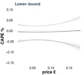
(a)

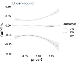
(b)

Figure 10: Fitted CAPE of waste demands at each price level. Fitted CAPE in the left (right) panel are estimated using CAPE lower-bounds (upper-bounds) of 95% confidence intervals.

Figure 11 reports effect heterogeneity across price levels, ceteris paribus. Price effects on the y-axis (CAPE kg) are estimated as quantity changes for a one cent price increase. CAPE heterogeneity varies at low versus high prices, ceteris paribus: a one cent price increase reduces UW by on average 10.8 kg at low prices vs. 14.2 kg at high prices, ceteris paribus. Higher prices lead to increased recycling by on average 6.8 kg at low prices vs. 11.6 kg at high prices. The remaining UW reductions are due to TW reductions.

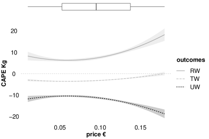
(a)

Figure 11: Fitted price effects on waste demands (CAPE kg) as quantity changes for a one euro cent price increase.

Figure 12 reports effect heterogeneity across prices by pre-policy RW levels, ceteris paribus. Effect heterogeneity is statistically significant only at high prices: municipalities recycling little before policy have generally higher elasticities, ceteris paribus, by on average 1.4 percent points.

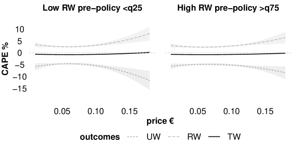
(a)

Figure 12: Fitted price semi-elasticities (CAPE) of waste demands by pre-policy recycling levels. Thresholds q25 and q75 indicate first (248 kg) and third (344 kg) quartiles of annual recycling per capita.

D.3 Distribution of policy effects on municipal costs

(a)

Figure 14: Distribution of policy Effects on Municipal Costs (EMC$>$0 indicate cost savings) for all observed municipalities after one, two, and three years of policy adoption in €  per capita. The y-axis refers to the number of treated and yet-to-be-treated municipalities.

Appendix E Robustness and Sensitivity

E.1 Possible unaccounted-for heterogeneity and spillovers

Waste tourism.–Violation of the no spillover assumption (SUTVA) could possibly come from waste tourism, namely, households may discharge their waste for free in surrounding municipalities without PAYT. I geocoded neighbors as never-treated units sharing a border with treated units. The remaining untreated units represent the control group. In order to estimate causal effects of PAYT on waste amounts of surrounding municipalities without PAYT, I use the RF running the R-learner described in Section 2.2. I find that PAYT has no significant effect on the waste amounts collected in surrounding municipalities on average. As a further robustness check, I re-estimate causal effects for PAYT municipalities excluding neighbors from the control group, finding no significant change in estimates. As in other empirical studies (e.g. Carattini et al., 2018; Allers and Hoeben, 2010; Dijkgraaf and Gradus, 2004), waste tourism is not relevant on any significant scale.

System effects.– Unaccounted-for heterogeneity may threaten identification. Adoption of different PAYT systems (e.g. volume versus weight) may have heterogeneous effects on waste generation. In the sample, about 7% of treated units pay per weight, 16% per bag, 72% per emptying, and 5% have a mixed system. I first test for whether the included covariates can explain system adoption. Second, I test for significant differences in price elasticities between systems.

Using all covariates, I predict system choices by RF for classification. I find that the included observables can predict (out of sample) system choices correctly for most municipalities. How do municipal characteristics affect system choices? Evidence provided by manufacturers of PAYT technology (e.g., magnetic cards, tags and RFID readers) suggests that system choices are driven by three main factors. First, proximity: neighboring municipalities may either share the same waste collection company or influence each other through information dissemination. Second, population density: sparsely populated municipalities are more likely to adopt weight systems (PartItalia, 2020). Third, geography: physical characteristics of the territory such as uphills and one-way roads impact transportation costs and collection modes.

I run a multinomial logit regression in order to assess whether observables can partly explain the choice of the adopted PAYT system. These are: population size (Population), distance to neighboring PAYT municipalities (Km to PAYT city), population density (Population density), and urbanization level (Medium/High/Low) as described in Table LABEL:table:var_desc in Appendix B. In particular, I specify urbanization levels as urban, peri-urban, semi-peripheral, and very peripheral (the reference category) based on travel times (t) from each municipality to the closest urban center. Table 8 shows the results including all treated observations in the first policy year. The dummy for weight systems is the reference choice.

Table 8: Average partial effect estimates of multinomial logit regression. Weight systems are the reference choice. Very peripheral areas (t$>$75’) are the reference category for geographic dummies.

	Dependent variable:
	emptying	bag	mixed
	(1)	(2)	(3)
Population	$-$0.085∗∗∗	$-$0.076∗∗	0.032
	(0.032)	(0.036)	(0.022)
Population density	0.009∗	0.011∗∗	0.011∗∗
	(0.005)	(0.005)	(0.005)
Km to PAYT city	$-$0.006	$-$0.017∗	$-$0.073
	(0.008)	(0.010)	(0.046)
Peripheral(40<t<75’)	1.189∗	1.655∗∗∗	28.377∗∗∗
	(0.663)	(0.000)	(0.663)
Semi-peripheral(20<t<40’)	$-$21.713∗∗∗	5.599∗∗∗	4.797∗∗∗
	(0.924)	(0.952)	(0.962)
Semi-urban(t<20’)	$-$24.078∗∗∗	2.523∗∗∗	2.132∗∗∗
	(0.699)	(0.718)	(0.781)
Peri-urban	$-$24.819∗∗∗	1.111∗∗	$-$36.060∗∗∗
	(1.618)	(0.525)	(0.000)
Urban	$-$20.275∗∗∗	4.625∗∗∗	$-$5.571∗∗∗
	(1.097)	(0.912)	(0.223)
Constant	36.339∗∗∗	13.313∗∗∗	0.799
	(1.145)	(0.980)	(0.706)
Observations	194	194	194
Year and area dummies	Yes	Yes	Yes
Akaike Inf. Crit.	284.558	284.558	284.558
Note:	∗p$<$0.1; ∗∗p$<$0.05; ∗∗∗p$<$0.01

Results show that lower population density (Population density) significantly increases the probability to adopt weight programs over any other, as expected. Higher populated municipalities (Population) are more likely to implement weight vs. bag/emptying programs, perhaps to exploit returns to scale. Information dissemination effects (Km to PAYT city) positively increase the choice of bag programs. Less peripheral municipalities are more likely to adopt bag systems over weight systems, and highly urbanized municipalities are more likely to adopt weight systems over emptying or mixed systems.

Next, I test for effect heterogeneity. Table 9 reports pairwise mean comparison tests (Games and Howell, 1976).

PAYT system	dUW	s.e.	p-value	dRW	s.e.	p-value	dTW	s.e.	p-value
emptying - bag	0.12	0.27	0.96	0.47	0.24	0.18	0.55	0.23	0.06
mixed - bag	0.19	0.52	0.98	0.56	0.46	0.59	0.62	0.44	0.47
weight - bag	0.76	0.52	0.44	0.16	0.46	0.98	1.06	0.44	0.07
mixed - emptying	0.07	0.48	1.00	0.09	0.42	1.00	0.07	0.40	1.00
weight - emptying	0.64	0.48	0.52	-0.31	0.42	0.87	0.50	0.40	0.57
weight - mixed	0.57	0.66	0.81	-0.40	0.57	0.89	0.44	0.55	0.85

Table 9: Pairwise comparison of price elasticities (CAPE) on waste amounts by PAYT system: Mean differences (dUW, dRW, dTW in kg per euro cent), standard errors and p-values estimated by Tukey-Kramer’s method (1956).

Mean differences are overall statistically insignificant at conventional confidence levels. Estimates only suggest that bag-based systems are (weakly) associated to larger reductions of total waste (significant at the 10% level), namely, price semi-elasticities on total waste are 0.55 and 1.06 kg higher (in absolute value) than with emptying- and weight-based systems, respectively. Overall, my study does not point towards significant differences in price elasticities between PAYT systems.

E.2 Robustness to alternative assumptions

I compare my average estimates to (i) the binary treatment case, which assumes no effect heterogeneity in prices; (ii) the two-way (event-study-like) fixed effects regression, which assumes no effect heterogeneity, and selection based on time-constant variables; and (iii) penalized linear regression methods known as LASSO, which assumes no effect heterogeneity, sparsity and linearity in a high-dimensional set of covariates. Binary treatment case.–The binary case assumes that the policy has homogeneous effects across prices, and that policy adoption is homogeneous in prices. Table 10 reports average price effects (APE) estimated as average effects of a binary treatment at the mean price level ($ATE/\bar{P}$).

	Continuous		Binary
Year	UW kg	s.e.	UW kg	s.e.
1	-7.38	1.30	-7.60	2.55
2	-8.86	1.03	-11.3	1.97
3	-11.5	1.53	-16.5	1.08

Table 10: Continuous APE vs. Binary APE estimates (kg) at the mean price (ATE/$\bar{P}$) from (level-level) residual-on-residual regression with year clustered standard errors.

Results show that mean elasticities (APE) on UW are overestimated by 28% on average relative to the continuous treatment case. Why does this happen? The forest kernel assigns similarity weights to units based on a residual-on-residual regression that ignores the price variation and uses a binary indicator instead. Hence, the algorithm may place units adopting high and low prices in the same neighborhood, and assign the same prediction to both units. However, I have shown that price responses at high and low prices are not the same, and the sources of effect heterogeneity differ.

Two-way fixed effects regression.–When the timing of treatment varies across units, Difference-in-Differences (DiD) designs are commonly extended to allow for dynamic average treatment effects by including leads and lags of treatment as regressors (Jacobson et al., 1993). These dummy variables allow policy effects to vary by the number of years relative to separation from policy. Figure 15 presents the results from a dynamic (event-study-like) DiD regression estimated using a standard two-way (unit and time) fixed effects model. The regression includes three leads and lags, and uses the second (unaffected) lead before policy (-2) as a baseline dummy. Since potentially relevant covariates are many and partly collinear, and there is no a priori guidance on which one to exclude, this DiD only controls for time-invariant waste generation determinants captured by municipal fixed effects. Figure 15 plots lead and lagged average price effect (APE) estimates (continuous treatment) with their confidence intervals. Black dots represent statistically significant effects at $5\%$, and vertical dotted lines indicate the policy adoption year.

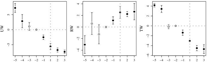
(a)

Figure 15: Dynamic DiD estimates (2010-2015, $n=19,982$) of average price effects (APE kg) on UW, RW, TW with year and unit fixed effects. Clustered standard errors (Driscoll and Kraay, 1994). Statistical significance (5%) indicated by black dots.

Results show that APE on UW are underestimated by 29% on average (see first panel of Figure 15). Moreover, standard event study pretrend tests (Autor, 2003) present evidence of non-parallel trends, thus, a bias in the estimation of average price elasticities. There are at least two possible sources of bias. First, unaccounted-for time-varying effects on the outcomes (Bueno and Valente, 2019). Second, heterogeneous treatment effects (De Chaisemartin and D’Haultfœuille, 2020). Due to staggered policy adoption, APE represent weighted averages of effects computed using both treated and untreated outcomes, which may not allow for a comparison with my estimates. Re-weighting the estimator according to De Chaisemartin and D’Haultfœuille (2020) gives, however, similar results and the bias persists. Therefore, bias may be due to effect heterogeneity across (covariate-specific) groups which are ex-ante unknown. RF methods allow for a data-driven way to estimate these groups and detect ex-post the relevant heterogeneities.

LASSO.–Similarly to RF, doubly robust LASSO regression estimates the APE after removing the correlation of covariates with outcomes and prices. Yet, differently from RF, it assumes causal effect homogeneity and, typically, linearity in covariates (Athey et al., 2017; Belloni et al., 2017). I find that my APE estimates are almost insensitive to these assumptions when differences in covariates are effectively adjusted. Yet, while RF allow to consistently estimate unit level causal effects and identify effect heterogeneity (Athey et al., 2019), doubly robust LASSO regression is suited for estimation of average treatment effects (Belloni et al., 2014).

Summary.–Table 11 summarizes all APE estimates by estimation method. Residualized reg via RF is my main estimation method; residualized reg via RF (bin.) assumes no heterogeneity in prices; dynamic fixed effects (FE) assumes constant APE and selection due to time-constant variables; double selection and residualized LASSO reg assume constant APE and linearity after effectively removing differences in covariates.

Method/APE estimates	UW kg	s.e.	RW kg	s.e.	TW kg	s.e.
residualized reg via RF	-11.50	1.50	8.10	2.20	-2.70	0.90
residualized reg via RF (bin.)	-16.50	1.10	13.0	2.20	-3.20	2.90
dynamic FE reg	-7.40	0.30	2.70	0.70	-4.70	0.50
dynamic FE reg (re-weighted)	-9.06	0.98	3.96	0.76	-5.10	0.40
double selection LASSO reg	-9.30	0.40	9.40	0.60	-1.00	0.50
residualized LASSO reg	-9.00	1.30	8.80	1.00	-1.00	1.30

Table 11: Method comparison: APE estimates in the third policy year. Estimates represent average kg changes in waste for a one cent price increase.

References

- Abadie and Imbens (2016) Abadie, A. and G. W. Imbens (2016). Large sample properties of matching estimators for average treatment effects. Econometrica 74(1), 235–267.
- Allers and Hoeben (2010) Allers, M. and C. Hoeben (2010). Effects of unit-based garbage pricing: A differences-in-differences approach. Environmental Resource Economics 45(3), 405–28.
- Athey and Imbens (2016) Athey, S. and G. Imbens (2016). Recursive partitioning for heterogeneous causal effects. PNAS 113(27), 7353–7360.
- Athey et al. (2017) Athey, S., G. Imbens, T. Pham, and S. Wager (2017). Estimating average treatment effects: Supplementary analyses and remaining challenges. American Economic Review 107(5), 278–281.
- Athey et al. (2019) Athey, S., J. Tibshirani, and S. Wager (2019). Generalized random forests. The Annals of Statistics 47(2), 1148–1178.
- Athey and Wager (2018) Athey, S. and S. Wager (2018). Estimation and inference of heterogeneous treatment effects using random forests. Journal of the American Statistical Association 113(523), 1228–1242.
- Athey and Wager (2019) Athey, S. and S. Wager (2019). Estimating treatment effects with causal forests: An application. Observational Studies 5(2), 37–51.
- Autor (2003) Autor, D. (2003). Outsourcing at will: The contribution of unjust dismissal doctrine to the growth of employment outsourcing. Journal of Labor Economics 21(1), 1–42.
- Batllevell and Hanf (2008) Batllevell, M. and K. Hanf (2008). The fairness of payt systems: Some guidelines for decision-makers. Waste Management 28, 2793–2800.
- Bel and Gradus (2016) Bel, G. and R. Gradus (2016). Effects of unit-based pricing on the waste collection demand: A meta-regression analysis. Resource and Energy Economics 44, 169–182.
- Belloni et al. (2017) Belloni, A., V. Chernozhukov, I. Fernández-Val, and C. Hansen (2017, January). Program evaluation and causal inference with high-dimensional data. Econometrica 85(1), 233–298.
- Belloni et al. (2014) Belloni, A., V. Chernozhukov, and C. Hansen (2014). Inference on treatment effects after selection amongst high-dimensional controls. Review of Economic Studies 81(2), 608–650.
- Breiman (2001) Breiman, L. (2001). Random forests. Machine Learning 45(1), 5–32.
- Bucciol et al. (2015) Bucciol, A., N. Montinari, and M. Piovesan (2015). Do not trash the incentive! Monetary incentives and waste sorting. The Scandinavian Journal of Economics 117(4), 1204–1229.
- Bueno and Valente (2019) Bueno, M. and M. Valente (2019). The effects of pricing waste generation: A synthetic control approach. Journal of Environmental Economics and Management 96, 274–285.
- Callan and Thomas (2006) Callan, S. and J. Thomas (2006). Analysing demand for disposal and recycling services: A system approach. East Economic Journal 31, 221–240.
- Callan and Thomas (1999) Callan, S. J. and J. M. Thomas (1999). Adopting a unit pricing system for municipal solid waste: Policy and socioeconomic determinants. Environmental Resource Economics 14(4), 503–518.
- Carattini et al. (2018) Carattini, S., A. Baranzini, and R. Lalive (2018). Is taxing waste a waste of time? Evidence from a Supreme Court decision. Ecological Economics 148, 131–151.
- Cecere et al. (2014) Cecere, G., S. Mancinelli, and M. Mazzanti (2014). Waste prevention and social preferences: the role of intrinsic and extrinsic motivations. Ecological Economics 107, 163–176.
- Central Maine (2015) Central Maine (2015). China moves ahead with pay-as-you-throw referendum. Available at http://www.centralmaine.com/2015/09/21/china-moves-ahead-with-pay-as-you-throw-referendum.
- Chernozhukov et al. (2017) Chernozhukov, V., D. Chetverikov, M. Demirer, E. Duflo, C. Hansen, W. Newey, and J. Robinson (2017). Double/debiased machine learning for treatment and structural parameters. The Econometrics Journal 21, C1–C68.
- Christensen et al. (2021) Christensen, P., P. Francisco, E. Myers, and M. Souza (2021, 08). Decomposing the wedge between projected and realized returns in energy efficiency programs. The Review of Economics and Statistics, 1–46.
- Conover (1971) Conover, W. J. (1971). Practical Nonparametric Statistics. New York: John Wiley & Sons.
- CONSEA (2019) CONSEA (2019). The quantity-based waste tariff (in Italian). CONSEA Waste Services and Consulting. Available at http://www.consea.eu/la-tariffa-puntuale-dieci-domande-e-risposte-per-capire-meglio-di-cosa-si-tratta.
- Croissant and Millo (2008) Croissant, Y. and G. Millo (2008). Panel data econometrics in R: The plm package. Journal of Statistical Software 27(2), 1–43.
- Crump et al. (2009) Crump, R. K., V. J. Hotz, G. W. Imbens, and O. A. Mitnik (2009). Dealing with limited overlap in estimation of average treatment effects. Biometrika 96(1), 187–199.
- Davis and Heller (2017) Davis, J. and S. Heller (2017, May). Using causal forests to predict treatment heterogeneity: An application to summer jobs. American Economic Review 107(5), 546–50.
- De Chaisemartin and D’Haultfœuille (2020) De Chaisemartin, C. and X. D’Haultfœuille (2020). Two-way fixed effects estimators with heterogeneous treatment effects. American Economic Review 110(9), 2964–96.
- Dijkgraaf and Gradus (2004) Dijkgraaf, E. and R. H. J. M. Gradus (2004). Cost savings in unit-based pricing of household waste: The case of The Netherlands. Resource and Energy Economics 26(4), 353–371.
- Dijkgraaf and Gradus (2009) Dijkgraaf, E. and R. H. J. M. Gradus (2009). Environmental activism and dynamics of unit-based pricing systems. Resource and Energy Economics 31(1), 13–23.
- Driscoll and Kraay (1994) Driscoll, J. C. and A. C. Kraay (1994). Consistent covariance matrix estimation with spatially dependent panel data. Review of Economics and Statistics 80(4), 549–560.
- Dunlap et al. (2000) Dunlap, R. E., K. D. Van Liere, A. G. Mertig, and R. E. Jones (2000). New trends in measuring environmental attitudes: Measuring endorsement of the new ecological paradigm: A revised nep scale. Journal of Social Issues 56(3), 425–442.
- Facchini (2020) Facchini, M. (2020). Precious waste: Quantity-based tariffs and separate collection are worth it (in Italian). Altraeconomia 225. Available at https://altreconomia.it/tariffa-puntuale-raccolta-differenziata/.
- Fullerton and Kinnaman (1996) Fullerton, D. and C. T. Kinnaman (1996). Household responses to pricing garbage by the bag. The American Economic Review 86(4), 971–984.
- Fullerton and Kinnaman (2000) Fullerton, D. and C. T. Kinnaman (2000). Garbage and recycling with endogenous local policy. Journal of Urban Economics 48(3), 419–442.
- Games and Howell (1976) Games, P. A. and J. F. Howell (1976). Pairwise multiple comparison procedures with unequal N’s and/or variances: A Montecarlo study. Journal of Educational Statistics 1, 13–125.
- Gilli et al. (2018) Gilli, M., S. Mancinelli, and F. Nicolli (2018). Household waste management: Some insights from behavioural economics. Cham: Palgrave Pivot, Economics and finance collection.
- Giraud (2015) Giraud, C. (2015). Introduction to High-Dimensional Statistics. Monographs on Statistics and Applied Probability 139, CRC Press - Taylor & Francis Group.
- Gradus et al. (2019) Gradus, R., G. C. Homsy, L. Liao, and M. E. Warner (2019). Which us municipalities adopt pay-as-you-throw and curbside recycling? Resources, Conservation and Recycling 143, 178–183.
- Grossmann et al. (1974) Grossmann, D., J. F. Hudson, and D. Marks (1974). Waste generation models for solid waste collection. Journal of the Environmental Engineering Division 100(6), 1219–1230.
- Hirano and Imbens (2004) Hirano, K. and G. Imbens (2004). The propensity score with continuous treatments. Applied Bayesian Modeling and Causal Inference from Incomplete-Data Perspectives, Chapter 7, Wiley Series in Probability and Statistics.
- Huang et al. (2011) Huang, J.-C., J. M. Halstead, and S. B. Saunders (2011). Managing municipal solid waste with unit-based pricing: Policy effects and responsiveness to pricing. Land Economics 87(4), 645–660.
- Imai and van Dyk (2004) Imai, K. and D. van Dyk (2004). Causal inference with general treatment regimes: Generalizing the propensity score. Journal of the American Statistical Association 99, 854–866.
- Imbens (2000) Imbens, G. (2000). The role of the propensity score in estimating dose-response functions. Biometrika 87(3), 706–710.
- Imbens and Rubin (2015) Imbens, G. and D. Rubin (2015). Causal Inference for Statistics, Social, and Biomedical Sciences - Chapter 14 Assessing Overlap in Covariate Distributions, Volume III. Cambridge University Press.
- ISPRA (2019) ISPRA (2019). Urban waste report. Italian National Institute for Environmental Protection and Research.
- ISTAT (2011) ISTAT (2011). Population and housing census. ISTAT - National Institute of Statistics. Data available at http://dati-censimentopopolazione.istat.it.
- ISTAT (2018) ISTAT (2018). Crimes against environment and landscape: Public prosecutor offices data. ISTAT - National Institute of Statistics. Available at http://www.istat.it/it/archivio/218648.
- Jacobson et al. (1993) Jacobson, L. S., R. J. LaLonde, and D. G. Sullivan (1993). Earnings losses of displaced workers. The American Economic Review 83(4), 685–709.
- Jenkins et al. (2003) Jenkins, R. R., S. A. Martinez, K. Palmer, and M. J. Podolsky (2003). The determinants of household recycling: A material-specific analysis of recycling program features and unit pricing. Journal of Environmental Economics and Management 45(2), 294–318.
- Kinnaman (2014) Kinnaman, C. T. (2014). Understanding the economics of waste: Drivers, policies, and external costs. International Review of Environmental and Resource Economics 8, 281–320.
- Kinnaman (2006) Kinnaman, T. C. (2006). Examining the justification for residential recycling. Journal of Economic Perspectives 20(4), 219–32.
- Kinnaman (2017) Kinnaman, T. C. (2017). The economics of residential solid waste management. Routledge.
- Kinnaman and Fullerton (1995) Kinnaman, T. C. and D. Fullerton (1995). Garbage, recycling, and illicit burning or dumping. Journal of Environmental Economics and Management 29(1), 78–91.
- Kramer (1956) Kramer, C. Y. (1956). Extension of multiple range tests to group means with unequal numbers of replications. Biometrics 12(3), 307–310.
- Legambiente (2017) Legambiente (2017). The quantity-based waste tariff: Systems and application methods (in Italian). Ecoforum Lombardia. Available at http://www.legambiente.it/sites/default/files/docs/2_-_la_tariffa_puntuale_sistemi_e_metodi_di_applicazione_g._ghiringhelli.pdf.
- Levene (1960) Levene, H. (1960). Robust tests for equality of variances. Contributions to Probability and Statistics: Essays in Honor of Harold Hotelling.
- Miranda and Bauer (1996) Miranda, M. L. and S. Bauer (1996). The urban performance of unit pricing: An analysis of variable rates for residential garbage collection in urban areas. The U.S. Environmental Protection Agency. Report prepared for the Office of Policy, Planning, and Evaluation.
- Nie and Wager (2021) Nie, X. and S. Wager (2021). Quasi-oracle estimation of heterogeneous treatment effects. Biometrika (108), 299–319.
- PartItalia (2020) PartItalia (2020). PAYT: The importance of the different systems (in Italian). Retrieved from raccoltapuntualefacile.com then substituted with http://www.partitalia.com/.
- Priest (2020) Priest, B. C. (2020). Peaking interest: How awareness drives the effectiveness of time-of-use electricity pricing. Journal of the Association of Environmental and Resource Economists 7(1).
- Richardson and Havlicek (1978) Richardson, R. A. and J. H. Havlicek (1978). Economic analysis of the composition of household solid wastes. Journal of Environmental Economics and Management 5(1), 103–111.
- Robinson (1988) Robinson, P. (1988). Root-n-consistent semiparametric regression. Econometrica 56(4), 931–954.
- Rosenbaum and Rubin (1983) Rosenbaum, P. and D. Rubin (1983). The central role of the propensity score in observational studies for causal effects. Biometrika 70(1), 41–55.
- Rubin (1974) Rubin, D. B. (1974). Estimating causal effects of treatments in randomized and nonrandomized studies. Journal of Educational Psychology 5(5), 688–701.
- Sexton and Laake (2009) Sexton, J. and P. Laake (2009). Standard errors for bagged and random forest estimators. Computational Statistics and Data Analysis 53(3), 801–811.
- Skumatz (2008) Skumatz, L. (2008). Pay as you throw in the U.S.: Implementation, impacts, and experience. Waste Management 28(12), 2778–2785.
- Tibshirani et al. (2018) Tibshirani, J., S. Athey, S. Wager, R. Friedberg, L. Miner, and M. Wright (2018). grf: Generalized random forests (beta). R package version 0.10.1. Available at http://CRAN.R-project.org/package=grf.
- Usui (2009) Usui, T. (2009). Does a rebound effect exist in solid waste management? Critical Issues in Environmental Taxation 7, 413–422.
- Van Houtven and Morris (1999) Van Houtven, G. L. and G. E. Morris (1999). Household behavior under alternative pay-as-you-throw systems for solid waste disposal. Land Economics 75(4), 515–537.
- Wertz (1976) Wertz, K. L. (1976). Economic factors influencing households’ production of refuse. Journal of Environmental Economics and Management 2(4), 263–272.
- Wilcoxon (1945) Wilcoxon, F. (1945). Individual comparisons by ranking methods. Biometrics Bulletin 1(6), 80–83.