Extreme Wave Runup on a Steep Coastal Profile

Abstract

It is shown that very steep coastal profiles can give rise to unexpectedly large wave events at the coast. We combine insight from exact solutions of a simplified mathematical model with photographs from observations at the Norwegian coast near the city of Haugesund. The results suggest that even under moderate wave conditions, very large run-up can occur at the shore.

I Introduction

In the present work, we are interested in the interaction of ocean waves with steep offshore topography such as encountered in some areas at the Norwegian coast. If surface waves propagate on such a steep bottom slope, they experience only slight amplification until very close to shore. However, just before they reach the beach face, the waves receive a large boost in amplitude which can lead to an explosive run-up on the shore. As this large run-up may seem wholly unexpected to the casual observer, it may constitute a potentially hazardous situation.

It is well known that the Norwegian coast especially in the south and the west features a multitude of fjords Klemsdal (1982). These rocky cliffs often continue past the waterline, and may drop to several hundred meters depth, cutting through the continental shelf as submarine valleys. This landscape was formed by glaciers during the last ice age. Indeed, it is well known that fjords developed due to glaciers’ capability of eroding below the sea level Klemsdal (1982); Johnson (1919), leaving deep submerged valleys when the ice age came to a close and melting was completed.

In some cases, these valleys are offshore of the present shoreline, and there are some places today where coastal platforms give way to very steep seaward slopes carved by these thick glaciers. In fact it is not unusual to see $200$ or $300$ meter drops of the sea bed over a distance of a few hundred meters. These steeply sloping shores typically consist of bedrock which has been smoothed by the glacial ice and is rather immune to erosion and littoral processes. In fact, wide stretches of the coast have not been filled with mud and other sediments, and the rocks remain exposed. As a result, this coast is generally classified as primary coast Klemsdal (1982), similar to coasts in other places around the word such as New Zealand and the northernmost part of the East Coast of the United States Johnson (1919).

Further offshore, the Norwegian coast features very irregular bathymetry which dissipates much of the incoming wave energy through wave focusing, shoaling and local breaking Grue (1992); Falnes (1993); Chawla, Özkan-Haller, and Kirby (1998). However, some long waves of moderate amplitude and steepness are able to pass the rugged offshore topography relatively unscathed and reach the coast. If these long waves hit an area with sharply sloping coastal profiles, even waves of relatively small amplitude can lead to large run-up. In what follows, in section II, we report observations of waves made at a site with a sharp, nearly $1:1$ drop from the water line. In section III, we detail a mathematical model capable of predicting large run-up from a moderate-sized offshore wavefield in the case of bathymetry featuring a steep slope such as seen at the observation site. The results are discussed in section IV.

Figure 1: Bathymetric chart of sea bed near Bleivika lighthouse. The depth contours run nearly parallel to the shore, and feature a steep drop from the shoreline to about $200$m depth. © Kartverket.
Used with permission from The Norwegian Mapping Authority.

II Observations

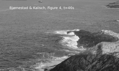
Observations were made at a site near the Norwegian city of Haugesund. As shown in Figure 1, the bathymetry near the coast features a steep drop to about $200$m right from the waterline. Indeed, it can be seen in the schematic of a cross-section of the site in Figure 2 that the slope is very steep, about $1:1$. Due to the very steep slope, it is common for waves to exhibit surging breaking, such as defined in Dean and Dalrymple (1984); Galvin (1968); Grilli, Svendsen, and Subramanya (1997). However, as waves of slightly larger amplitude quickly shoal on the steep slope they sometimes reach the point of plunging almost as soon as they can be made out as a large wave. One such example is shown in Figure 3. Under the rough conditions prevailing when the photos in Figure 3 were taken, energetic waves crash into the rocks, creating large areas of turbulent flow. The accompanying foam and spray immediately alert the observer to the fact that wave conditions are serious, and caution must be exercised. On the other hand, the conditions in Figure 4 were mostly calm with little visible swell, and only a small chop due to a moderate local wind. A few small patches of foam are visible which appear to be remnants of previous waves interacting with the jagged rocks, or white-capping due to local wind gusts. The smaller swell waves were just lapping the shore, and the limited foam and absence of spray do not signal any danger. As a slightly larger swell wave approaches and shoals, the subsequent wave run-up appears extreme against the backdrop of otherwise benign wave and weather conditions. An example of such explosive run-up is shown in Figure 4, and one may argue that the flooding of the rocks may happen unexpectedly to a non-initiated observer.

Figure 2: Schematic of sea bed near Stemmevika.

Figure 3: This figure shows four snapshots of wave conditions at $59.48^{\circ}$ N, $13.44^{\circ}$ E on January 16th, 2020. Upper left: $t=105$s, upper right: $t=115$s, lower left: $t=120$s, lower right: $t=124$s.

II.1 Observations on January 16th, 2020

Observations were made from a location near the lighthouse Bleivika indicated by a star on the map in Figure 1. We used an Olymp Mark III E camera to shoot $4$K video clips. Individual frames from those clips are shown in the figures below. Wave conditions were monitored using operational wave forecasts from two sources. First, the NOAA site gave an estimate of the significant waveheight and the peak period for the general area using an operational version of Wavewatch III. On this day, the significant waveheight was in the range $2-2.5$m, and the peak wave period was about $10$s.

For local conditions, a forecast provided by the The BarentsWatch Centre was consulted. Near the coast, the waves had already encountered several shoals, and the waveheight and wave periods were somewhat smaller. The wind speed was above $9$m/s so there was a significant wind sea component in addition to swell. Most waves were surging breakers, but some waves were steep enough to break before reaching the shore. Figure 3 shows a wave developing along the steep sloping bottom. It can be seen that the waveheight develops quickly, and in this case the wave is large enough for the wave to plunge before it hits the rocky shore. This situation would not pose a danger to the casual observer since wave conditions were not calm.

II.2 Observations on January 29th, 2020

In this case, the wave forecasts from NOAA and Barentswatch Centre estimated the local significant waveheight to be just above $1$m, with a maximum waveheight of about $2$m. Visually, conditions were rather calm, as also borne out from a study of Figure 4. However, there was swell from a distant storm, and the peak wave period was about $13$s (i.e. wavelength of $\sim 260$m based on linear wave theory). The authors were at the site for about $90$ minutes, and the visually measured wave period was on average about $9-13$s, though some waves were as short as $6$s, and some waves were longer than $13$s.

The rock which is in view in Figure 4 stayed dry for the most part, though in the $90$ minutes we were present, it was flooded $3$ times. In fact, as far as we can tell, what typically seemed to happen was that a group of waves arrived which had slightly higher than normal waveheight, and the rock was flooded not by the first, but by the second and/or third wave in the group. After such an incident, the conditions went back to normal. Indeed, it is well known that swell will organize into wave groups (see Thompson, Nelson, and Sedivy (1984); Longuet-Higgins (1984); Masselink (1995) and references therein), so the situation above would have to be expected. As mentioned above, in the $90$-minute observational period, there were three waves that flooded the rock, two of these in one wave group, and one in another wave group.

Figure 4 shows a wave crest at $t=15$s (relative time in the video), an approximately flat surface at $t=18$s, and the wave trough at $t=21$s. This was a relatively unspectacular wave with a small waveheight hitting the rock. The next wave (not shown) already has a larger amplitude, but stops short of the rock. Finally, $25$ seconds later, at $t=46$s the third wave crest hits the rock, flooding the top of the rock almost entirely. Using tide tabulations, and a local elevation map, the run-up can be estimated to be about $3.8$m.

III Mathematical model

In the following, it will be shown that a comparatively simple mathematical model can be used to understand how relatively small waves can lead to significant and unexpected run-up if encountering a steep slope. For this purpose, we will use the shallow-water system

$$h_{t}+\left(uh\right)_{x}= 0,$$ (1)

$$u_{t}+uu_{x}+g\left(h+b\right)_{x}= 0,$$ (2)

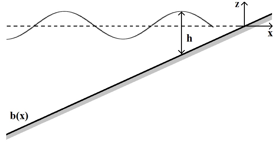
where $h(x,t)$ is the total depth of the fluid, $u(x,t)$ is the average horizontal velocity, $g$ is the gravitational acceleration, and $b(x)$ is the bottom profile. In the present case, we define the bathymetry by $b(x)=\theta x$. The surface elevation is then given by $\eta(x,t)=h(x,t)+\theta x$.

This system is able to describe long waves in shallow water, and it is possible to find exact solutions in the presence of non-constant bathymetry which enable us to make predictions of the development of the waterline. Exact solutions of $2\times 2$ systems of conservation laws are classically obtained using a hodograph transformation, where dependent and independent variables are interchanged Courant and Friedrichs (1999). In the presence of bathymetry, it is somewhat more difficult to find the requisite change of variables than in the case of constant coefficients. Nevertheless, an appropriate hodograph transformation was found by Carrier and Greenspan Carrier and Greenspan (1958), and there have been a number of works seeking to extend and generalize that idea (see Synolakis (1987); Antuono and Brocchini (2007); Didenkulova and Pelinovsky (2011); Bjørnestad and Kalisch (2017); Bjørnestad (2020); Rybkin et al. (2020) and references therein).

Figure 4: This figure shows four snapshots of wave conditions at $59.48^{\circ}$ N, $13.44^{\circ}$ E on January 29th, 2020. Upper left: wave trough at $t=15$s, upper right: mean water level at $t=18$s, lower left: wave crest at $t=21$s, lower right: wave crest at $t=46$s.

Figure 5: Offshore wavefield and run-up on a $1:1$ slope for two different offshore wave conditions. In the left panel, we have offshore amplitude $0.459$m and run-up $2.548$m. In the right panel, we have offshore amplitude $0.918$m and run-up $5.097$m.

In the present situation, it is important that the system be solved in dimensional coordinates in order to understand the influence of the steep bottom slope. For the convenience of the reader, the construction of the exact solutions is explained in the appendix. As demonstrated in the appendix, the independent variables $\lambda$ and $\sigma$ are introduced through a hodograph transformation. These variables do not have a clear physical meaning. However, using separation of variables, an exact solution can be specified with the help of a “potential” $\phi$ defined in terms of the velocity $u$ by the relation $u=\frac{1}{\sigma}\phi_{\sigma}$. In terms of the potential, the solution has the form

$$\phi\left(\sigma,\lambda\right)=\frac{A}{k}J_{0}(k\sigma)\cos(k\lambda).$$ (3)

Here $J_{0}$ is the zeroth-order Bessel function of the first kind, and $A$ and $k$ are arbitrary constants. Using the potential $\phi$, an expression for $x(\sigma,\lambda)$ is found in the form

$$x=\frac{1}{2g\theta}\Big{(}\frac{1}{2}\phi_{\lambda}-u^{2}-\frac{\sigma^{2}}{8}\Big{)},$$ (4)

and $t(\sigma,\lambda)$ can be expressed as

$$t=\frac{1}{2g\theta}\Big{(}\lambda-2u\Big{)}.$$ (5)

The surface elevation $\eta=h+\theta x$ is given by

$$\eta=\frac{1}{2g}\Big{(}\frac{1}{2}\phi_{\lambda}-u^{2}\Big{)}.$$ (6)

Note that in contrast to the solution provided in Carrier and Greenspan (1958), the slope $\theta$ appears explicitly in the final solution.

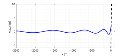
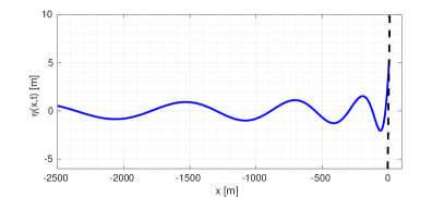
This solution can now be used to investigate the run-up for various wave conditions. In Figure 5, an exact solution is plotted with a steep slope of $\theta=1$. In the left panel, we choose $A=100\>\frac{m^{2}}{s^{2}}$ and $k=0.04\>\frac{s}{m}$ (we emphasize that even though $A$ and $k$ feature units, there is no clear physical meaning assigned to these constants) in the solution to obtain an offshore amplitude $0.459$m, and run-up $2.548$m. The steepness, defined as $2\pi A/L$ where $L$ is the wavelength is $0.0029$. In the right panel, we chose $A=200\>\frac{m^{2}}{s^{2}}$ and $k=0.04\>\frac{s}{m}$to plot an offshore amplitude $0.918$m with a steepness of $0.0059$ and run-up of $5.097$m. In Table 1 the run-up for four different offshore amplitudes for waves with a period $T=8$s is recorded. The values of $A$ used in the table are $50\>\frac{m^{2}}{s^{2}}$, $100\>\frac{m^{2}}{s^{2}}$, $200\>\frac{m^{2}}{s^{2}}$,$300\>\frac{m^{2}}{s^{2}}$. The 8s period is found by choosing $k=0.04\>\frac{s}{m}$. The amplification factor between offshore amplitude and run-up is $5.5$.

Table 1: Run-up for four different offshore amplitudes for waves with period $T=8$s and varying steepness. The amplification factor between offshore amplitude and run-up is $5.5$.

Amplitude (offsh.) [m]	Steepness (offsh.)	Period [s]	Run-up [m]
0.229	0.0015	8	1.274
0.459	0.0029	8	2.548
0.918	0.0059	8	5.097
1.377	0.0088	8	7.645

IV Discussion

In this work, the run-up of waves on a steep slope has been studied through field observations at the Norwegian coast and a mathematical model. The observations presented here point to the possibility that extreme wave run-up may occur during otherwise benign conditions. The effect of the large run-up is further enhanced by the more moderate slope of the coast above the waterline (see Figure 2), leading to a large area of flooding, such as shown in Figure 4.

The mathematical model used here also shows that unusually large run-up can be realized on a steep slope by small offshore amplitudes. Indeed, it is evident from Table 1 that a moderate rise in offshore amplitude from $0.459$m to $0.918$m may lead to a difference of more than $2.5$m in the run-up height. A still moderate wave amplitude of $1.377$m can lead to run-up height of $7.648$m.

In summary, both observations and the shallow-water theory show that large run-up may occur under otherwise inconspicuous conditions. The two approaches do not give a perfect quantitative match because of the inherent quantitative uncertainty in the observations, and because some of the shorter waves observed are only shallow-water waves once they enter the coastal slope. Nevertheless both observation and mathematical theory clearly show large amplification of the waves as they approach the shore, and it is clear that an observer focusing on offshore conditions may be taken by surprise as moderate waves experience such strong amplification and subsequent explosive run-up on the shore.

In the present work we have focused on a very steep $1:1$ slope where the bathymetry has a decisive effect on the wave evolution and the resulting run-up. It appears that in many previous works on extreme wave events in shallow water, a gently sloping bottom was assumed. This is the case in particular in studies on so-called sneaker waves, which are generally taken to be large run-up events on gentle beaches García-Medina et al. (2018); Nikolkina and Didenkulova (2011); Didenkulova et al. (2006). On the other hand, there are some studies on unusually large waves, or freak waves in shallow water, but not near the shore. For example in Didenkulova and Pelinovsky (2011); Nikolkina and Didenkulova (2011), the authors describe freak waves occurrences in the nearshore zone, and in Soomere and Engelbrecht (2006); Soomere (2010), the authors look at wave interaction phenomena as possible route to freak wave development. In Zhang et al. (2019), laboratory experiments and numerical simulations are used to explain the occurrence of freak waves. In the situation considered in these works, even though the waves are in shallow water, the bathymetry does not exert a major effect on the fashion in which large wave events develop.

In contrast, a strong influence of the bathymetry on the wave conditions was found in Stefanakis, Dias, and Dutykh (2011), where resonant behavior due to irregular underwater topography was considered and also in Trulsen, Zeng, and Gramstad (2012); Gramstad et al. (2013). However, the slopes considered in these works were still much more gentle than the steep $1:1$ bathymetry considered in the present work. On the other hand, run-up on a vertical wall, such as a sea cliff were studied in Mirchina and Pelinovsky (1984); Carbone et al. (2013).

There is a large literature on rogue or freak waves (see Ochi (1998); Onorato et al. (2001); Kharif and Pelinovsky (2003); Dysthe, Krogstad, and Müller (2008); Fedele et al. (2016); Donelan and Magnusson (2017); Didenkulova (2020) and the references therein). It is not clear whether the present phenomenon should be classified as a freak wave event since at least in theory it can be predicted if measurements of the offshore wavefield are available. Indeed it would be interesting to conduct field measurements at this or a similar site, such as reported on in the in-depth study Dodet et al. (2018). However with the conditions in this case such as the extreme slope, the slippery rocks and small tidal range, it appears challenging to obtain reliable measurements.

*

Appendix A Exact solutions for the shallow-water equations

The shallow-water equations (1) and (2) are to be solved on a domain such as indicated in Figure 6. As suggested in Gavrilyuk, Makarenko, and Sukhinin (2017), a gas dynamics analogy may be used to find the eigenvalues and the Riemann invariants for the shallow-water system. Using (1) to rewrite (2) as

$$\left(hu\right)_{t}+\left(hu^{2}+p(h)\right)_{x}=-gh\theta,$$ (7)

where $p(h)=\frac{1}{2}gh^{2}$, a similarity to the gas-dynamic equations for a barotropic gas can be seen if we consider $P(h)$ as the “pressure” and $h$ as the “density”. For more details, the reader may consult Courant and Friedrichs (1999). Indeed, with this analogy, the eigenvalues are $\lambda_{1,2}=u\pm c$ and the Riemann invariants can be found to be

$$\alpha= u+\int\frac{c(h)}{h}\>dh+g\theta t,$$ (8)

$$\beta= u-\int\frac{c(h)}{h}\>dh+g\theta t,$$ (9)

where $c$ is defined by $c^{2}=\frac{dp}{dh}$. The last term on the right hand side is due to the bathymetry. The system can then be written in terms of the characteristic variables $\alpha=u+2\sqrt{gh}+g\theta t$ and $\beta=u-2\sqrt{gh}+g\theta t$ as

$$\left\{\frac{\partial}{\partial t}+\left(u+\sqrt{gh}\right)\frac{\partial}{\partial x}\right\}\left(u+2\sqrt{gh}+g\theta t\right) =0,$$ (10)

$$\left\{\frac{\partial}{\partial t}+\left(u-\sqrt{gh}\right)\frac{\partial}{\partial x}\right\}\left(u-2\sqrt{gh}+g\theta t\right) =0.$$ (11)

Figure 6: Definition sketch for mathematical model, including the slope $b(x)$ and the water depth $h(x,t)=\eta(x,t)-b(x)$.

The hodograph transform can be effected by implicit differentiation of the equations (10) and (11) and using the dependent variables $x=x(\alpha,\beta)$ and $t=t(\alpha,\beta)$ instead of $\alpha=\alpha(x,t)$ and $\beta=\beta(x,t)$. Assuming a non-zero Jacobian $\frac{\partial(x,t)}{\partial(\alpha,\beta)}$, the equations (10) and (11) become

$$x_{\beta}-\lambda_{1}t_{\beta}= 0,$$ (12)

$$x_{\alpha}-\lambda_{2}t_{\alpha}= 0.$$ (13)

In order to obtain a linear set of equation, we define new independent variables $\lambda=\alpha+\beta$ and $\sigma=\alpha-\beta$. The systems then appears as

$$x_{\lambda}-ut_{\lambda}+\sqrt{gh}\>t_{\sigma}= 0,$$ (14)

$$x_{\sigma}-ut_{\sigma}+\sqrt{gh}\>t_{\lambda}= 0.$$ (15)

Assuming that $x_{\sigma\lambda}=x_{\lambda\sigma}$ and $t_{\sigma\lambda}=t_{\lambda\sigma}$, the two equations reduce to

$$u_{\sigma}t_{\lambda}-u_{\lambda}t_{\sigma}-\left(\sqrt{gh}\right)_{\sigma}t_{\sigma}+\left(\sqrt{gh}\right)_{\lambda}t_{\lambda}\\ =\sqrt{gh}\>\left(t_{\sigma\sigma}-t_{\lambda\lambda}\right).$$ (16)

Using the expressions for the new independent variables yields

$$\frac{\lambda}{2} =u+g\theta t,$$ (17)

$$\frac{\sigma}{4} =\sqrt{gh}.$$ (18)

By using (17) and (18), expressions for $u_{\sigma}$, $u_{\lambda}$, $\left(\sqrt{gh}\right)_{\sigma}$ and $\left(\sqrt{gh}\right)_{\lambda}$ can be found and (16) turns into the linear wave equation

$$\sigma\left(t_{\lambda\lambda}-t_{\sigma\sigma}\right)-3t_{\sigma}=0.$$ (19)

Using the expression (17) for $\lambda$ together with an appropriate potential function $u=\frac{1}{\sigma}\phi_{\sigma}$, the equation (19) can be rewritten as

$$\left(\sigma\phi_{\sigma}\right)_{\sigma}-\sigma\phi_{\lambda\lambda}=0.$$ (20)

Using separation of variables, we are able to find an exact solution which is bounded as $\sigma\rightarrow 0$. This solution can be written as

$$\phi\left(\sigma,\lambda\right)=\frac{A}{k}J_{0}(k\sigma)\cos(k\lambda),$$ (21)

where $J_{0}$ are the Bessel function of first kind of order zero, and $A$ and $k$ are constants.

With this solution in hand, an expression for $x(\sigma,\lambda)$ is found in the form

$$x=\frac{1}{2g\theta}\Big{(}\frac{1}{2}\phi_{\lambda}-u^{2}-\frac{\sigma^{2}}{8}\Big{)},$$ (22)

and $t(\sigma,\lambda)$ can be expressed as $t=\frac{1}{2g\theta}\left(\lambda-2u\right)$. The surface elevation $\eta=h+\theta x$ is then given by $\eta=\frac{1}{2g}\left(\frac{1}{2}\phi_{\lambda}-u^{2}\right)$.

References

- Klemsdal (1982) T. Klemsdal, “Coastal classification and the coast of Norway,” Norwegian Journal of Geography 36, 129–152 (1982).
- Johnson (1919) D. W. Johnson, Shore Processes and Shoreline Development (Wiley, 1919).
- Grue (1992) J. Grue, “Nonlinear water waves at a submerged obstacle or bottom topography,” Journal of Fluid Mechanics 244, 455–476 (1992).
- Falnes (1993) J. Falnes, “Research and development in ocean-wave energy in Norway,” in Proceedings of International Symposium on Ocean Energy Development, edited by H. Kondo (Cold Region Port and Harbor Engineering Research Center, Murora, 1993) pp. 27–39.
- Chawla, Özkan-Haller, and Kirby (1998) A. Chawla, H. T. Özkan-Haller, and J. Kirby, “Spectral model for wave transformation and breaking over irregular bathymetry,” J. Waterw. Port Coast. Ocean Eng. 124, 189–198 (1998).
- Dean and Dalrymple (1984) R. G. Dean and R. A. Dalrymple, Water Wave Mechanics for Scientists and Engineers (World Scientific, 1984).
- Galvin (1968) C. J. Galvin, “Breaker type classification on three laboratory beaches,” J. Geoph. Res. 73, 3651–3659 (1968).
- Grilli, Svendsen, and Subramanya (1997) S. T. Grilli, I. A. Svendsen, and R. Subramanya, “Breaking criterion and characteristics for solitary waves on slopes,” J. Waterways Port Coastal Ocean Engng. 123, 102–112 (1997).
- Note (1) NOAA WAVEWATCH III, https://polar.ncep.noaa.gov/waves/, National Weather Service, USA.
- Note (2) The BarentsWatch Centre, https://www.barentswatch.no/en/services/Wave-forecasts/, Wave forcast.
- Thompson, Nelson, and Sedivy (1984) W. Thompson, A. Nelson, and D. Sedivy, “Wave group anatomy of ocean wave spectra,” in Coastal Engineering Proceedings (1984).
- Longuet-Higgins (1984) M. Longuet-Higgins, “Statistical properties of wave groups in a random sea state,” Philosophical Transactions of the Royal Society of London 312, 219–250 (1984).
- Masselink (1995) G. Masselink, “Group bound long waves as a source of infragravity energy in the surf zone,” Continental Shelf Research 15, 1525–1547 (1995).
- Courant and Friedrichs (1999) R. Courant and K. O. Friedrichs, Supersonic flow and shock waves (Springer, 1999).
- Carrier and Greenspan (1958) G. Carrier and H. Greenspan, “Water waves of finite amplitude on a sloping beach,” Journal of Fluid Mechanics 4, 97–109 (1958).
- Synolakis (1987) C. Synolakis, “The runup of solitary waves,” Journal of Fluid Mechanics 185, 523–545 (1987).
- Antuono and Brocchini (2007) M. Antuono and M. Brocchini, “The boundary value problem for the nonlinear shallow water equations,” Studies in Applied Mathematics 119, 73–93 (2007).
- Didenkulova and Pelinovsky (2011) I. Didenkulova and E. Pelinovsky, “Rogue waves in nonlinear hyperbolic systems,” Nonlinearity 24, R1–R18 (2011).
- Bjørnestad and Kalisch (2017) M. Bjørnestad and H. Kalisch, “Shallow water dynamics on linear shear flows and plane beaches,” Phys. Fluids 29, 073602 (2017).
- Bjørnestad (2020) M. Bjørnestad, “Shallow water dynamics on linear shear flows and plane beaches,” Wave Motion (2020).
- Rybkin et al. (2020) A. Rybkin, D. Nicolsky, E. Pelinovsky, and M. Buckel, “The generalized Carrier-Greenspan transform for the shallow water system with arbitrary initial and boundary conditions,” Water Waves (2020).
- García-Medina et al. (2018) G. García-Medina, H. T. Özkan-Haller, P. Ruggiero, R. A. Holman, and T. Nicolini, “Analysis and catalogue of sneaker waves in the US pacific northwest between 2005 and 2017,” Natural Hazards 94, 583–603 (2018).
- Nikolkina and Didenkulova (2011) I. Nikolkina and I. Didenkulova, “Rogue waves in 2006-2011,” Nat. Hazards Earth Syst. Sci. 11, 2913–2924 (2011).
- Didenkulova et al. (2006) I. I. Didenkulova, A. V. Slunyaev, E. N. Pelinovsky, and C. Kharif, “Freak waves in 2005,” Nat. Hazards Earth Syst. Sci. 6, 1007–1015 (2006).
- Soomere and Engelbrecht (2006) T. Soomere and J. Engelbrecht, “Weakly two-dimensional interaction of solitons in shallow water,” Eur. J. Mech. B / Fluids 25, 636–648 (2006).
- Soomere (2010) T. Soomere, “Rogue waves in shallow water,” Eur. Phys. J.-Spec. Top. 185, 81–96 (2010).
- Zhang et al. (2019) J. Zhang, M. Benoit, O. Kimmoun, A. Chabchoub, and H. Hsu, “Statistics of extreme waves in coastal waters: large scale experiments and advanced numerical simulations,” Fluids 4, 99 (2019).
- Stefanakis, Dias, and Dutykh (2011) T. S. Stefanakis, F. Dias, and D. Dutykh, “Local run-up amplification by resonant wave interactions,” Physical Review Letters 107, 124502 (2011).
- Trulsen, Zeng, and Gramstad (2012) K. Trulsen, H. Zeng, and O. Gramstad, “Laboratory evidence of freak waves provoked by non-uniform bathymetry,” Phys. Fluids 24, 097101 (2012).
- Gramstad et al. (2013) O. Gramstad, H. Zeng, K. Trulsen, and G. Pedersen, “Freak waves in weakly nonlinear unidirectional wave trains over a sloping bottom in shallow water,” Phys. Fluids 25, 122103 (2013).
- Mirchina and Pelinovsky (1984) N. Mirchina and E. Pelinovsky, “Increase in the amplitude of a long wave near a vertical wall,” Izvestiya, Atmospheric and Oceanic Physics 20, 252–253 (1984).
- Carbone et al. (2013) F. Carbone, D. Dutykh, J. M. Dudley, and F. Dias, “Extreme wave runup on a vertical cliff,” Geophysical Research Letters 40, 3138–3143 (2013).
- Ochi (1998) M. K. Ochi, Ocean Waves, the Stochastic Approach (Cambridge University Press, 1998).
- Onorato et al. (2001) M. Onorato, A. Osborne, M. Serio, and S. Bertone, “Freak waves in random oceanic sea states,” Physical Review Letters 86, 5831 (2001).
- Kharif and Pelinovsky (2003) C. Kharif and E. Pelinovsky, “Physical mechanisms of the rogue wave phenomenon,” Eur. J. Mech. B/Fluids 22, 603–634 (2003).
- Dysthe, Krogstad, and Müller (2008) K. Dysthe, H. E. Krogstad, and P. Müller, “Oceanic rogue waves,” Ann. Rev. Fluid. Mech 40, 287–310 (2008).
- Fedele et al. (2016) F. Fedele, J. Brennan, S. De Leon, J. Dudley, and F. Dias, “Real world ocean rogue waves explained without the modulational instability,” Scientific reports 6, 27715 (2016).
- Donelan and Magnusson (2017) M. A. Donelan and A. K. Magnusson, “The making of the Andrea wave and other rogues,” Scientific reports 7, 44124 (2017).
- Didenkulova (2020) E. Didenkulova, “Catalogue of rogue waves occurred in the world ocean from 2011 to 2018 reported by mass media sources,” Ocean Coast. Management 188, 105076 (2020).
- Dodet et al. (2018) G. Dodet, F. Leckler, D. Sous, F. Ardhuin, J. F. Filipot, and S. Suanez, “Wave runup over steep rocky cliffs,” Journal of Geophysical Research: Oceans 123, 7185–7205 (2018).
- Gavrilyuk, Makarenko, and Sukhinin (2017) S. L. Gavrilyuk, N. I. Makarenko, and S. V. Sukhinin, Waves in Continuous Media (Springer International Publishing, 2017).