A consistent and conservative Phase-Field method for multiphase incompressible flows

Abstract

In the present study, a consistent and conservative Phase-Field method, including both the model and scheme, is developed for multiphase flows with an arbitrary number of immiscible and incompressible fluid phases. The consistency of mass conservation and the consistency of mass and momentum transport are implemented to address the issue of physically coupling the Phase-Field equation, which locates different phases, to the hydrodynamics. These two consistency conditions, as illustrated, provide the “optimal” coupling because (i) the new momentum equation resulting from them is Galilean invariant and implies the kinetic energy conservation, regardless of the details of the Phase-Field equation, and (ii) failures of satisfying the second law of thermodynamics or the consistency of reduction of the multiphase flow model only result from the same failures of the Phase-Field equation but are not due to the new momentum equation. Physical interpretation of the consistency conditions and their formulations are first provided, and general formulations that are obtained from the consistency conditions and independent of the interpretation of the velocity are summarized. Then, the present consistent and conservative multiphase flow model is completed by selecting a reduction consistent Phase-Field equation. Several novel techniques are developed to inherit the physical properties of the multiphase flows after discretization, including the gradient-based phase selection procedure, the momentum conservative method for the surface force, and the general theorems to preserve the consistency conditions on the discrete level. Equipped with those novel techniques, a consistent and conservative scheme for the present multiphase flow model is developed and analyzed. The scheme satisfies the consistency conditions, conserves the mass and momentum, and assures the summation of the volume fractions to be unity, on the fully discrete level and for an arbitrary number of phases. All those properties are numerically validated. Numerical applications demonstrate that the present model and scheme are robust and effective in studying complicated multiphase dynamics, especially for those with large-density ratios.

Keywords: Multiphase incompressible flows; Phase-Field model; Consistent scheme; Mass conservation ; Momentum conservation; large-density ratio

1 Introduction

Multiphase flows are ubiquitous in real-world problems. Interactions among different fluid phases and evolution of their interfaces are strongly coupled and, as a result, introduce complicated dynamics that casts challenges of solving the problems. In the present study, we consider that fluid phases have constant (but not necessarily identical) densities, viscosities, and interfacial tensions. Many efforts have been paid on cases including two immiscible fluid phases, and these cases are commonly referred to as the two-phase flows. Under the “one-fluid formulation” framework (Tryggvasonetal2011, ; ProsperettiTryggvason2007, ), where the dynamics of the two fluid phases is governed by a single set of transport equations in the entire domain, many numerical models or methods for the two-phase flows have been developed, greatly improved, and successfully implemented. Examples of those numerical models or methods are the Front-Tracking method (UnverdiTryggvason1992, ; Tryggvasonetal2001, ), the Level-Set method (OsherSethian1988, ; Sussmanetal1994, ; SethianSmereka2003, ; Gibouetal2018, ), the Conservative Level-Set method (OlssonKreiss2005, ; Olssonetal2007, ; ChiodiDesjardins2017, ), the Volume-of-Fluid (VOF) method (HirtNichols1981, ; ScardovelliZaleski1999, ; Popinet2009, ; OwkesDesjardins2017, ), the “THINC” method (Xiaoetal2005, ; Iietal2012, ; XieXiao2017, ; Qian2018, ), the Phase-Field (or Diffuse-Interface) method (Andersonetal1998, ; Jacqmin1999, ; Shen2011, ; Huangetal2020, ), the continuous surface force (CSF) (Brackbilletal1992, ), the ghost fluid method (GFM) (Fedkiwetal1999, ; Lalanneetal2015, ), and the balanced-force algorithm (Francoisetal2006, ; Popinet2018, ).

Recent studies are moving towards cases including three fluid phases or, more generally, an arbitrary number of fluid phases. Compared to the two-phase problems, the three-phase or the general $N$-phase ($N\geqslant 1$) flows cast some additional challenges in locating phases and interfaces and in modeling interfacial tensions and moving contact lines. The interface reconstruction schemes in the Volume of Fluid (VOF) and Moment of Fluid (MOF) methods for the two-phase flows are extended to the three-phase cases, e.g., in (Schofieldetal2009, ; Schofieldetal2010, ; Francois2015, ; PathakRaessi2016, ), and become more involved. One can expect that those schemes become more and more complicated as the number of phases increases. The Level-Set method is also extended to the three- or $N$-phase problems, e.g., in (Smithetal2002, ; Losassoetal2006, ; Starinshaketal2014, ), by simply adding more Level-Set functions. However, special cares have to be paid on overlaps or voids introduced by independently advecting the Level-Set functions, and on the issue of mass conservation.

The Phase-Field method is popularly used to model multiphase dynamics because of its simplicity and effectiveness. It is characterized by introducing a small but finite interface thickness. The Phase-Field method includes thermodynamical compression and diffusion related to a free energy functional, and their competition helps to preserve the interface thickness. Phases are labeled by a set of order parameters governed by the Phase-Field equation. Many Cahn-Hilliard Phase-Field equations for the three-phase problems are developed, e.g., in (BoyerLapuerta2006, ; Boyeretal2010, ; Kim2007, ), and some of them have been extended to the $N$-phase cases, e.g., in (BoyerMinjeaud2014, ; Kim2009, ; LeeKim2015, ; Kim2012, ). The three-phase moving contact lines on a solid wall are modeled in (ZhangWang2016, ) and (Zhangetal2016, ), using the wall energy functional and the geometrical formulation, respectively. Multiphase Allen-Cahn and Cahn-Hilliard Phase-Field equations including effects of pairwise interfacial tensions are developed in (WuXu2017, ). A $N$-phase conservative Allen-Cahn Phase-Field equation is developed in (KimLee2017, ), extended from its two-phase counterpart in (BrasselBretin2011, ). A series of studies on the Phase-Field modeling of $N$-phase incompressible flows has been performed by Dong (Dong2014, ; Dong2015, ; Dong2017, ; Dong2018, ), where not only the Cahn-Hilliard Phase-Field equation but also the contact angle boundary condition is considered. Early studies only require the Phase-Field equation to follow the mass conservation of each phase and to ensure the summation of the volume fractions of the phases to be unity. Recent studies have realized the significance of the so-called consistency of reduction(BoyerLapuerta2006, ; BoyerMinjeaud2014, ; Dong2017, ; Dong2018, ), because this principle eliminates the possibility of producing fictitious phases. General theories and discussions about developing a reduction consistent Phase-Field equation are available in (BoyerLapuerta2006, ; Boyeretal2010, ; BoyerMinjeaud2014, ; LeeKim2015, ; Dong2017, ; Dong2018, ; WuXu2017, ) and the references therein.

The first issue considered in the present study is developing a physical momentum equation that governs the motion of the multiphase fluid mixture, provided a mass conservative Phase-Field equation. In previous studies, most attention was paid to developing the Phase-Field equation that captures phase locations, while physical coupling between the Phase-Field equation and the hydrodynamics was less studied. Once the Phase-Field equation is obtained, the hydrodynamics was included by solving the Navier-Stokes equation:

$$\frac{\partial(\rho\mathbf{u})}{\partial t}+\nabla\cdot(\rho\mathbf{u}\otimes\mathbf{u})=-\nabla P+\mathbf{f},$$ (1)

or its equivalent form. Here, $\rho$ is the density of the fluid mixture, $\mathbf{u}$ is the velocity and is divergence-free, i.e., $\nabla\cdot\mathbf{u}=0$, $P$ is the pressure, and $\mathbf{f}$ denotes any forces other than the pressure gradient. Such a strategy of coupling the Phase-Field equation to the hydrodynamics is extended from the so-called modified model H using the Cahn-Hilliard Phase-Field equation in the two-phase cases, and has been popularly used in the two-phase flows, e.g., (GuermondQuartapelle2000, ; Kim2005, ; Dingetal2007, ; DongShen2012, ; Huangetal2019, ), and more recently in the three-phase or $N$-phase flows, e.g., (BoyerLapuerta2006, ; Boyeretal2010, ; BoyerMinjeaud2014, ; Kim2007, ; Kim2009, ; Kim2012, ; LeeKim2015, ; KimLee2017, ; ZhangWang2016, ; Zhangetal2016, ; Abadi2018, ). It should be noted that validity of the above coupling strategy is rooted in the presumption that the density of the fluid mixture is governed by

$$\frac{\partial\rho}{\partial t}+\nabla\cdot(\rho\mathbf{u})=0,$$ (2)

and we call Eq.(2) the sharp-interface mass conservation equation in the present study. However, $\rho$ is never solved from Eq.(2) but instead computed algebraically from $\sum_{p=1}^{N}\rho_{p}C_{p}$ where $\rho_{p}$ and $C_{p}$ are the density and volume fraction of Phase $p$. We show in the present study that the algebraically computed mixture density can be contradicting to the sharp-interface mass conservation equation Eq.(2), in particular when the velocity is divergence-free. As a result, the Navier-Stokes equation Eq.(1) becomes inconsistent with the “actual” mass conservation equation of the mulitphase flow model, and can produce unphysical results. Such an issue in the two-phase flows was realized and addressed in our recent studies (Huangetal2020, ; Huangetal2020CAC, ), by proposing and successfully applying the consistency of mass conservation and the consistency of mass and momentum transport to the Cahn-Hilliard and conservative Allen-Cahn Phase-Field equations, respectively. Analyses in (Huangetal2020, ) show that violating those consistency conditions, such as using the modified model H, introduces sources that are proportional to the density difference of the two fluid phases in both the momentum and kinetic energy transports, and therefore results in unphysical velocity fluctuations and interface deformations in large-density-ratio problems. This emphasizes the significance of carefully considering the coupling between the Phase-Field equation and the hydrodynamics. Compared to the exiting Phase-Field based multiphase flow models using the divergence-free velocity and to our previous studies on the two-phase flows (Huangetal2020, ; Huangetal2020CAC, ), the present study lifts restrictions on the number of phases and on a specific Phase-Field equation, and has the following contributions to the aspect of modeling:

• The consistency of mass conservation and the consistency of mass and momentum transport are first applied to the general $N$-phase ($N\geqslant 1$) cases and to any Phase-Field equation that satisfies the mass conservation. The resulting formulations are therefore generally valid.

• Effects of the consistency of mass conservation and the consistency of mass and momentum transport on the kinetic energy conservation and the Galilean invariance of the momentum equation are analyzed in a formal way, regardless of the number of phases or details of the Phase-Field equation.

• The consistency of mass conservation and the consistency of mass and momentum transport provide the “optimal” coupling to the hydrodynamics in the sense that the second law of thermodynamics or the consistency of reduction of the multiphase flow model only relies on the corresponding properties of the Phase-Field equation.

• The physical interpretation of the consistency conditions and their formulations are first provided using the control volume analysis and mixture theory.

Thus, the consistency conditions are general, simple, and effective modeling principles for multiphase flows, and the rest is to develop or select a physically admissible Phase-Field equation. Here, we are not attempting to propose a new Phase-Field equation but choose the one in (Dong2018, ) to finalize the present consistent and conservative multiphase flow model, because that Phase-Field equation is fully reduction consistent, conserves the mass of individual phases, and eliminates local voids or overfilling. Although we limit our focus in the present study on models using the divergence-free velocity which can be interpreted as the “volume-averaged” velocity, there is another category of Phase-Field based multiphase flow models, like those in (LowengrubTruskinovsky1998, ; Shenetal2013, ; GuoLin2015, ; Shenetal2020, ; KimLowengrub2005, ; LiWang2014, ; Odenetal2010, ), using the “mass-averaged” velocity which is not divergence-free. The consistency conditions can also be applied to that circumstance. We further illustrate that, after implementing the consistency conditions, both categories of models produce the mass conservation equation equivalent to the one from the mixture theory, and share the same form of the momentum equation.

Another issue to be addressed in the present study is to preserve as many physical properties of a multiphase flow model as possible on the discrete level, in order to eliminate unphysical behaviors of numerical solutions. However, this part is still far from complete, particularly in the three- or $N$-phase cases, although some of those schemes are shown to satisfy a discrete energy law, e.g., in (Boyeretal2010, ; ZhangWang2016, ; WuXu2017, ), and to achieve mass conservation, e.g., in (Boyeretal2010, ; KimLee2017, ). For large-density-ratio problems, the so-called consistent schemes were developed for the two-phase flows, see, e.g., (Rudman1998, ; Bussmannetal2002, ; ChenadecPitsch2013, ; OwkesDesjardins2017, ) for the Volume-of-Fluid (VOF) method, (RaessiPitsch2012, ; Nangiaetal2019, ) for the Level-Set method, and (Huangetal2020, ; Huangetal2020CAC, ) for the Cahn-Hilliard and conservative Allen-Cahn Phase-Field equations, respectively. Since there are various Phase-Field equations developed for the multiphase flows and therefore numerical schemes that solve them, it is desirable to develop a unified framework that is applicable to an arbitrary number of phases, various Phase-Field equations for the multiphase flows, and different numerical methods that solve those Phase-Field equations, to obtain the consistent schemes. In the present study, we develop several novel techniques to satisfy the aforementioned consistency conditions, conserve the mass and momentum, and additionally assure the summation of the volume fractions to be unity. Those novel techniques that are first reported in the present study include:

• The gradient-based phase selection procedure is developed to remove mass change, fictitious phases, local voids, or overfilling, produced numerically by the convection term in the Phase-Field equation.

• The conservative method is developed to discretize the surface force that models interfacial tensions in the multiphase flows, which contributes to the conservation of momentum.

• General theorems, applicable to various Phase-Field equations and their discretization, are proposed to preserve the consistency conditions on the discrete level, which highlight correspondences of numerical operations in solving the Phase-Field and momentum equations.

Incorporating the above novel techniques to the second-order decoupled scheme in (Dong2018, ) for the Phase-Field equation and the second-order projection scheme in (Huangetal2020, ) for the momentum equation, we obtain the consistent and conservative scheme for the present mulitphase flow model. Moreover, we supplement the following analyses and proofs on the fully discrete level, which have not been reported in (Dong2018, ; Huangetal2020, ):

• The present scheme for the Phase-Field equation satisfies the consistency of reduction, conserves the mass of each phase, and also guarantees the summation of the volume fractions to be unity at every discrete location.

• The present scheme for the momentum equation conserves the momentum when the surface force is either neglected or computed by the conservative method, and recovers the single-phase dynamics discretely inside each bulk-phase region.

• The present scheme physically connects the discrete Phase-Field and momentum equations, following the consistency of mass conservation and the consistency of mass and momentum transport, and therefore solves advection (or translation) problems exactly with no restrictions on material properties or interface shapes.

The properties above are carefully validated by numerical experiments. Comparison studies illustrate productions of fictitious phases, local voids or overfilling, non-conservation of momentum, and unphysical velocity fluctuations and interface deformations, without implementing the novel techniques. It is worth mentioning that all those novel techniques, analyses, and proofs are generally valid for an arbitrary number of phases and dimensions. Applications of the present consistent and conservative model and scheme to the realistic multiphase flows demonstrate their robustness and capability of simulating multiphase dynamics even when there are significant density and/or viscosity ratios.

This article is organized as the following. In Section 2, after defining the multiphase problems, we implement the consistency conditions to obtain a physical momentum equation, illustrate the significance of satisfying the consistency conditions, and finally provide their physical interpretation. In Section 3, the novel techniques that help to preserve the physical properties of the multiphase flows are developed. In Section 4, the present consistent and conservative scheme, incorporating the novel techniques, is proposed and analyzed. In Section 5, the present multiphase flow model and scheme are validated by a series of numerical experiments, and then applied to various realistic multiphase flow problems. Finally, we conclude the present study in Section 6.

2 Definitions and governing equations

In this section, we first define the basic variables in the multiphase flow problems. Then, we implement the consistency of mass conservation to a generic form of the Phase-Field equation and derive the “actual” mass conservation equation and the consistent mass flux of the multiphase flow model. The momentum equation compatible with the “actual” mass conservation equation is obtained following the consistency of mass and momentum transport, and the significance of implementing these two consistency conditions are discussed. After that, we proceed to investigate the second law of thermodynamics and the consistency of reduction of the entire multiphase flow model. Finally, we select the fully reduction consistent Phase-Field equation in (Dong2018, ) to specify the present consistent and conservative multiphase flow model, and summarize the physical properties of the present model on the continuous level. At the end of this section, we provide physical interpretation to the consistency conditions, and illustrate that the consistency conditions and their resulting formulations fit in alternative multiphase flow models whose velocity is not necessarily divergence-free.

2.1 Basic definitions

Inside the domain of interest, there are $N$ ($N\geqslant 1$) immiscible and incompressible fluid phases. “Immiscible” means the phases are unable to form a homogeneous mixture, and “incompressible” means the densities of the phases are constant. The volume fraction of Phase $p$, denoted by $C_{p}$ here, is defined as the portion of Phase $p$ in a differential volume ($d(vol)_{p}$) over the same differential volume ($d(vol)$), i.e., $C_{p}=d(vol)_{p}/d(vol)$. Since no void or overfilling is allowed to be generated, the summation of the volume fractions over all the phases should be unity. Another popular choice to locate the phases is the volume fraction contrast, whose definition is

$$\phi_{p}=C_{p}-\sum_{q=1,q\neq p}^{N}C_{q}=2C_{p}-1,\quad 1\leqslant p\leqslant N,$$ (3)

and its range is from $-1$ to $1$. Correspondingly, the summation of the volume fraction contrasts is

$$\sum_{p=1}^{N}C_{p}=\sum_{p=1}^{N}\frac{1+\phi_{p}}{2}=1\quad\mathrm{or}\quad\sum_{p=1}^{N}\phi_{p}=(2-N).$$ (4)

Either the volume fractions $\left\{C_{p}\right\}_{p=1}^{N}$ or the volume fraction contrasts $\left\{\phi_{p}\right\}_{p=1}^{N}$ can be used as the order parameters in a Phase-Field method, and the latter case is considered in the present study unless otherwise specified.

The density and viscosity of Phase $p$ are $\rho_{p}$ ($\rho_{p}\geqslant 0$) and $\mu_{p}$ ($\mu_{p}\geqslant 0$), respectively. The density and viscosity of the fluid mixture are defined by

$$\rho=\sum_{p=1}^{N}\rho_{p}C_{p}=\sum_{p=1}^{N}\rho_{p}\frac{\phi_{p}+1}{2},$$ (5)

$$\mu=\sum_{p=1}^{N}\mu_{p}C_{p}=\sum_{p=1}^{N}\mu_{p}\frac{\phi_{p}+1}{2}.$$ (6)

The interfacial tension between Phases $p$ and $q$ is $\sigma_{p,q}$ ($1\leqslant p,q\leqslant N$), and there is no interfacial tension inside each phase. Thus, we have $\sigma_{q,p}=\sigma_{p,q}$ and $\sigma_{p,p}=0$. The contact angle of Phases $p$ and $q$ at a wall, measured inside Phase $p$, is $\theta_{p,q}^{W}$ ($1\leqslant p,q\leqslant N$). Consequently, we have $\theta_{p,q}^{W}+\theta_{q,p}^{W}=\pi$.

Without loss of generality, the Phase-Field equation is written as

$$\frac{\partial\phi_{p}}{\partial t}+\nabla\cdot(\mathbf{u}\phi_{p})=\nabla\cdot\mathbf{J}_{p},\quad 1\leqslant p\leqslant N,$$ (7)

where $\mathbf{u}$ is the velocity, and $\{\mathbf{J}_{p}\}_{p=1}^{N}$ are the diffusion fluxes of the order parameters. For those Phase-Field equations that include terms in a non-conservative form, like the conservative Allen-Can equation (RubinsteinSternberg1992, ; BrasselBretin2011, ), one can apply the consistent formulation (Huangetal2020CAC, ) and turn those terms into a conservative form. Therefore, Eq.(7) is adequate to represent all the equations that conserve the order parameters and therefore the mass of the phases. At the moment, explicit definition of $\{\mathbf{J}_{p}\}_{p=1}^{N}$ is not necessary, but we require $\sum_{p=1}^{N}\mathbf{J}_{p}=\mathbf{0}$. As a result, after summing Eq.(7) over all the phases and considering Eq.(4), we obtain that the velocity is divergence-free:

$$\nabla\cdot\mathbf{u}=0.$$ (8)

Further interpretation of such a divergence-free velocity and the requirement of $\sum_{p=1}^{N}\mathbf{J}_{p}=\mathbf{0}$ will be provided in Section 2.7. The divergence-free condition Eq.(8) is enforced by a Lagrange multiplier $P$, called the pressure.

Additionally, we assume that the Phase-Field equation Eq.(7) already satisfies the consistency of reduction, whose definition, similar to the one in (BoyerMinjeaud2014, ; Dong2018, ), is

• Consistency of reduction: A $N$-phase system should be able to recover the corresponding $M$-phase system $(1\leqslant M\leqslant N-1)$ when $(N-M)$ phases don’t appear.

Violating this consistency condition can easily generate fictitious phases in interfacial regions (BoyerMinjeaud2014, ; LeeKim2015, ). As demonstrated in (BoyerMinjeaud2014, ), generation of fictitious phases will significantly change the multiphase dynamics in problems having large density or viscosity ratios, in spite of the fact that amounts of the fictitious phases are small. This is because the density and viscosity of the fluid mixture is extensively modified by the fictitious phases. To obey this consistency condition, some requirements are posted to the diffusion fluxes $\{\mathbf{J}_{p}\}_{p=1}^{N}$ in the Phase-Field equation Eq.(7).

Theorem 2.1.

If and only if the formulation of the diffusion fluxes $\{\mathbf{J}_{p}\}_{p=1}^{N}$ in the Phase-Field equation Eq.(7) has the following two properties: (i) its value becomes zero for the absent phases, and (ii) it, for the present phases, recovers the corresponding formulation excluding contributions from the absent phases, then the Phase-Field equation Eq.(7) satisfies the consistency of reduction.

Proof.

Suppose the number of phases is $N$ ($N\geqslant 2$) and Phase $N$ is absent, i.e., $\phi_{N}\equiv-1$, the Phase-Field equation Eq.(7) becomes

$$\frac{\partial\phi_{N}}{\partial t}=-\underbrace{\nabla\cdot(\mathbf{u}\underbrace{\phi_{N}}_{-1})}_{-\nabla\cdot\mathbf{u}=0}+\nabla\cdot\underbrace{\mathbf{J}_{N}}_{0}=0\quad\mathrm{or}\quad\phi_{N}=-1\quad\forall t>0,$$

$$\frac{\partial\phi_{p}}{\partial t}+\nabla\cdot(\mathbf{u}\phi_{p})=\nabla\cdot\mathbf{J}_{p},\quad 1\leqslant p\leqslant(N-1).$$

Therefore, absent Phase $N$ remains absent. Since $\{\mathbf{J}\}_{p=1}^{N-1}$ recover the corresponding $(N-1)$-phase formulation excluding the contribution from absent Phase $N$, the Phase-Field equation for the present phases, i.e., Phases $1$-$(N-1)$, is identical to the one when there are only $(N-1)$ phases. Any other phase can be chosen as the absent phase and the above procedure can be repeated. As a result, the Phase-Field equation is reduction consistent. On the other hand, if the Phase-Field equation Eq.(7) is reduction consistent already, then, from the definition of the consistency of reduction, the diffusion fluxes need to have the two properties. ∎

From the requirement of $\sum_{p=1}^{N}\mathbf{J}_{p}=\mathbf{0}$ and the consistency of reduction of the Phase-Field equation, it is straightforward to deduce $\mathbf{J}_{p}=\mathbf{0}$ when there is only single Phase $p$ ($1\leqslant p\leqslant N$). Another possible consequence of violating this consistency condition is producing incorrect dynamics inside bulk-phase regions, and this will be discussed in more detail when considering the momentum equation in Section 2.5.

2.2 The mass conservation

As the density of the fluid mixture is computed from Eq.(5), instead of presuming that the mixture density is governed by the sharp-interface mass conservation equation Eq.(2), we follow the consistency of mass conservation which was proposed and successfully implemented in the two-phase flows (Huangetal2020, ). The definition of this consistency condition is:

• Consistency of mass conservation: The mass conservation equation should be consistent with the Phase-Field equation and the density of the fluid mixture. In this mass conservation equation, the consistent mass flux should lead to a zero mass source.

Following this consistency condition, one can, in general, reach the transport equation below for the density of the fluid mixture:

$$\frac{\partial\rho}{\partial t}+\nabla\cdot\mathbf{m}^{*}=S_{m^{*}},$$ (9)

after using Eq.(5) and Eq.(7), and noticing that the velocity is divergence-free, i.e., Eq.(8). Here, $\mathbf{m}^{*}$ is the mass flux and $S_{m^{*}}$ is the mass source. Depending on how the mass flux is defined, the mass source is determined correspondingly. For example, if the mass flux is defined as $\mathbf{m}^{*}=\rho\mathbf{u}$, then the corresponding mass source is $S_{m^{*}}=\sum_{p=1}^{N}\frac{\rho_{p}}{2}\nabla\cdot\mathbf{J}_{p}$. Therefore, the mixture density, in general, is not necessarily governed by the sharp-interface mass conservation equation Eq.(2). Instead, Eq.(9) is the “actual” mass conservation equation of the multiphase flow model.

As the “actual” mass conservation equation Eq.(9) is obtained, the next step is to specify the consistent mass flux $\mathbf{m}$ among various choices. The consistency of mass conservation points out that the corresponding mass source of the consistent mass flux is zero, i.e., $S_{m}=0$. As a result, Eq.(9) becomes

$$\frac{\partial\rho}{\partial t}+\nabla\cdot\mathbf{m}=0,$$ (10)

after using the consistent mass flux $\mathbf{m}$. Applying Eq.(10), Eq.(5), and Eq.(7), the divergence of the consistent mass flux is

$$\nabla\cdot\mathbf{m}=-\frac{\partial\rho}{\partial t}=-\frac{\partial}{\partial t}\sum_{p=1}^{N}\rho_{p}\frac{1+\phi_{p}}{2}=-\sum_{p=1}^{N}\frac{\rho_{p}}{2}\frac{\partial\phi_{p}}{\partial t}=\nabla\cdot\sum_{p=1}^{N}\frac{\rho_{p}}{2}(\mathbf{u}\phi_{p}-\mathbf{J}_{p}),$$ (11)

and therefore the consistent mass flux is

$$\mathbf{m}=\sum_{p=1}^{N}\frac{\rho_{p}}{2}(\mathbf{u}+\mathbf{u}\phi_{p}-\mathbf{J}_{p}).$$ (12)

It should be noted that one more $\mathbf{u}$ is added inside the parentheses of Eq.(12), due to the consistency of reduction. If only Phase $p$ appears, the consistent mass flux $\mathbf{m}$ should become $\rho_{p}\mathbf{u}$, which is true from Eq.(12) since $\phi_{p}=1$, $\{\phi_{q}\}_{q=1,q\neq p}^{N}=-1$, and $\{\mathbf{J}_{p}\}_{p=1}^{N}=\mathbf{0}$. On the other hand, if the consistent mass flux is defined as $\sum_{p=1}^{N}\frac{\rho_{p}}{2}(\mathbf{u}\phi_{p}-\mathbf{J}_{p})$, directly from Eq.(11), it becomes $\frac{1}{2}(\rho_{p}-\sum_{q=1,q\neq p}^{N}\rho_{q})\mathbf{u}$ when only Phase $p$ is present, and consequently violates the consistency of reduction. It should also be noted that the definition of the consistent mass flux in Eq.(12) is also consistent with the given example of Eq.(9) where $\mathbf{m}^{*}=\rho\mathbf{u}$ and $S_{m^{*}}=\sum_{p=1}^{N}\frac{\rho_{p}}{2}\nabla\cdot\mathbf{J}_{p}$. Since the velocity is divergence-free, the divergence of the consistent mass flux defined in Eq.(12) follows Eq.(11), and therefore the consistency of mass conservation is held.

To further simplify the formulations, we introduce the Phase-Field fluxes $\{\mathbf{m}_{\phi_{p}}=\mathbf{u}\phi_{p}-\mathbf{J}_{p}\}_{p=1}^{N}$ that include both the convection and diffusion fluxes in the Phase-Field equation, and we have the following theorem:

Theorem 2.2.

Given the Phase-Field fluxes $\{\mathbf{m}_{\phi_{p}}\}_{p=1}^{N}$ that satisfy the Phase-Field equation:

$$\frac{\partial\phi_{p}}{\partial t}+\nabla\cdot\mathbf{m}_{\phi_{p}}=0,\quad 1\leqslant p\leqslant N,$$ (13)

the corresponding consistent mass flux that satisfies the consistency of mass conservation is

$$\mathbf{m}=\sum_{p=1}^{N}\frac{\rho_{p}}{2}(\mathbf{u}+\mathbf{m}_{\phi_{p}}).$$ (14)

Formulations in Theorem 2.2 not only have a simpler form but also are more convenient to preserve the consistency of mass conservation in numerical practice, which will be seen in Section 3. Hereafter, the (actual) mass conservation equation is referred to Eq.(10) and the consistent mass flux is referred to Eq.(14). It is worth mentioning that Theorem 2.2 has no restrictions on the Phase-Field fluxes $\{\mathbf{m}_{\phi_{p}}\}_{p=1}^{N}$ (or the diffusion fluxes $\{\mathbf{J}_{p}\}_{p=1}^{N}$) in the Phase-Field equation. Therefore, it is generally applicable to different Phase-Field equations. Physical interpretation of the actual mass conservation equation Eq.(10) and the consistent mass flux Eq.(14) is provided in Section 2.7.

2.3 The momentum equation

As already indicated in Section 2.2, it is possible that the density of the fluid mixture is not governed by the sharp-interface mass conservation equation, i.e., Eq.(2). As a result, the Navier-Stokes equation Eq.(1) needs to be modified in order to be compatible with the “actual” mass conservation equation of the multiphase flow model. The question becomes what the corresponding momentum transport of the fluid mixture is provided the mass conservation equation written in Eq.(10). This question is answered by the consistency of mass and momentum transport which was proposed and successfully implemented in the two-phase flows (Huangetal2020, ). The definition of this consistency condition is:

• Consistency of mass and momentum transport: The momentum flux in the momentum equation should be the tensor product between the mass flux and the velocity, where the mass flux should be identical to the one in the mass conservation equation.

Following this consistency condition, the momentum equation governing the motion of the fluid mixture becomes

$$\frac{\partial(\rho\mathbf{u})}{\partial t}+\nabla\cdot\left(\mathbf{m}\otimes\mathbf{u}\right)=-\nabla P+\nabla\cdot\left[\mu(\nabla\mathbf{u}+\nabla\mathbf{u}^{T})\right]+\rho\mathbf{g}+\mathbf{f}_{s},$$ (15)

where $\otimes$ denotes the tensor product, $\mathbf{g}$ is the gravity, and $\mathbf{f}_{s}$ is the surface force modeling interfacial tensions. It should be noted that the inertia term in Eq.(15) is written in its conservative form, which is essential to achieve momentum conservation on the discrete level, and the consistent mass flux $\mathbf{m}$ obtained in Section 2.2 has been applied. The surface force $\mathbf{f}_{s}$ in the present study will be obtained after considering the energy law in Section 2.4, and it is shown in that section that the surface force is equivalent to a conservative form. Therefore, without considering the gravity, the momentum, i.e., $\int_{\Omega}\rho\mathbf{u}d\Omega$, is conserved by Eq.(15) even including effects of interfacial tensions.

The significance of implementing the consistency of mass conservation and the consistency of mass and momentum transport can be illustrated when considering the Galilean invariance of the momentum equation and the conservation of the kinetic energy.

Theorem 2.3.

If both the consistency of mass conservation and the consistency of mass and momentum transport are satisfied, then the momentum equation Eq.(15) is Galilean invariant.

Proof.

The Galilean transformation is

$$\mathbf{x}^{\prime}=\mathbf{x}-\mathbf{u}_{0}t,\quad t^{\prime}=t,\quad\mathbf{u}^{\prime}=\mathbf{u}-\mathbf{u}_{0},\quad f^{\prime}=f,\quad\nabla^{\prime}f^{\prime}=\nabla f,\quad\frac{\partial f^{\prime}}{\partial t^{\prime}}=\frac{\partial f}{\partial t}+\mathbf{u}_{0}\cdot\nabla f.$$

Here, $(\mathbf{x},t)$ is the fixed frame and $(\mathbf{x}^{\prime},t^{\prime})$ is the moving frame with respect to the fixed frame with a constant velocity $\mathbf{u}_{0}$. $f$ is a scalar variable measured in the fixed frame, while $f^{\prime}$ is the same variable measured in the moving frame. Applying the Galilean transformation, the momentum equation in the moving frame has the same form as the one in the fixed frame:

$$\frac{\partial(\rho^{\prime}\mathbf{u}^{\prime})}{\partial t^{\prime}}+\nabla^{\prime}\cdot\left(\mathbf{m}^{\prime}\otimes\mathbf{u}^{\prime}\right)+\nabla^{\prime}P^{\prime}-\nabla^{\prime}\cdot\left[\mu^{\prime}(\nabla^{\prime}\mathbf{u}^{\prime}+\nabla^{\prime}\mathbf{u^{\prime}}^{T})\right]-\rho^{\prime}\mathbf{g}^{\prime}-\mathbf{f}^{\prime}_{s}$$

$$=\underbrace{\left(\frac{\partial(\rho\mathbf{u})}{\partial t}+\nabla\cdot\left(\mathbf{m}\otimes\mathbf{u}\right)+\nabla P-\nabla\cdot\left[\mu(\nabla\mathbf{u}+\nabla\mathbf{u}^{T})\right]-\rho\mathbf{g}-\mathbf{f}_{s}\right)}_{\mathbf{0}}-\mathbf{u}_{0}\underbrace{\left(\frac{\partial\rho}{\partial t}+\nabla\cdot\mathbf{m}\right)}_{0}=\mathbf{0}.$$

The two parentheses group, respectively, the momentum equation Eq.(15) and the mass conservation equation Eq.(10) in the fixed frame, both of which are zero. Therefore, the momentum equation Eq.(15) satisfying the two consistency conditions is Galilean invariant. ∎

Corollary 2.3.1.

If the mechanical equilibrium in the hydrostatic state is reached, i.e.,

$$-\nabla P+\rho\mathbf{g}+\mathbf{f}_{s}=\mathbf{0},$$

then any homogeneous velocity is an admissible solution of the momentum equation Eq.(15).

Proof.

Suppose the velocity in the moving frame, i.e., $\mathbf{u}^{\prime}$, is zero, then the mechanical equilibrium is true in the moving frame. From the Galilean transformation, the velocity in the fixed frame becomes $\mathbf{u}=\mathbf{u}_{0}$, and the mechanical equilibrium is still valid. As a result, the left-hand side of the momentum equation Eq.(15) becomes $\mathbf{u}_{0}$ times the mass conservation equation Eq.(10) and therefore is zero. The right-hand side remains the viscous force which is again zero since there is no velocity gradient. Therefore, any homogeneous velocity $\mathbf{u}_{0}$ is the solution of the momentum equation Eq.(15) if the mechanical equilibrium is reached. ∎

Theorem 2.4.

If both the consistency of mass conservation and the consistency of mass and momentum transport are satisfied, then the momentum equation Eq.(15) implies the following kinetic energy equation:

$$\frac{\partial e_{K}}{\partial t}+\nabla\cdot\left(\mathbf{m}\frac{\mathbf{u}\cdot\mathbf{u}}{2}\right)=-\nabla\cdot(\mathbf{u}P)+\nabla\cdot[\mu(\nabla\mathbf{u}+\nabla\mathbf{u}^{T})\cdot\mathbf{u}]$$

$$-\frac{1}{2}\mu(\nabla\mathbf{u}+\nabla\mathbf{u}^{T}):(\nabla\mathbf{u}+\nabla\mathbf{u}^{T})+\rho\mathbf{u}\cdot\mathbf{g}+\mathbf{u}\cdot\mathbf{f}_{s}.$$

Here, $e_{K}=\frac{1}{2}\rho\mathbf{u}\cdot\mathbf{u}$ is the kinetic energy density.

Proof.

Performing the dot product between $\mathbf{u}$ and Eq.(15), and applying the integration by part, the right-hand side (RHS) of the kinetic energy equation is obtained. The left-hand side (LHS) of the kinetic energy equation is obtained from

$$\mathbf{u}\cdot\left(\frac{\partial(\rho\mathbf{u})}{\partial t}+\nabla\cdot(\mathbf{m}\otimes\mathbf{u})\right)=\frac{\partial e_{K}}{\partial t}+\nabla\cdot\left(\mathbf{m}\frac{1}{2}\mathbf{u}\cdot\mathbf{u}\right)+\frac{1}{2}\mathbf{u}\cdot\mathbf{u}\underbrace{\left(\frac{\partial\rho}{\partial t}+\nabla\cdot\mathbf{m}\right)}_{0}.$$

The right-most parentheses group the mass conservation equation Eq.(10) which therefore is zero. ∎

Corollary 2.4.1.

If all the forces except the pressure gradient are neglected and all the boundary integrals vanish with some proper boundary conditions, then the momentum equation Eq.(15) implies the kinetic energy conservation, i.e.,

$$\frac{dE_{K}}{dt}=\frac{d}{dt}\int_{\Omega}e_{K}d\Omega=0.$$

Proof.

Integrating the kinetic energy equation in Theorem 2.4 over domain $\Omega$, keeping only the first term on RHS, applying the integration by part, and dropping all the boundary integrals, then the kinetic energy conservation is obtained. ∎

Thanks to satisfying the consistency of mass conservation and the consistency of mass and momentum transport, the momentum equation Eq.(15) honors the physical properties in Theorem 2.3, Theorem 2.4, and their corollaries. The critical step in those proofs is to obtain the “actual” mass conservation equation which is zero because of the consistency of mass conservation. This is achieved by applying the consistent mass flux in the inertia term of the momentum equation, following the consistency of mass and momentum transport. Violating either of the consistency conditions results in failures of proving Theorem 2.3, Theorem 2.4, or their corollaries, and such a momentum equation will not only produce a problematic kinetic energy equation but also be Galilean variant. An informative example will be considering the usage of the Navier-Stokes equation Eq.(1) to govern the motion of the fluid mixture, which is equivalent to replacing the consistent mass flux $\mathbf{m}$ in Eq.(15) with $\mathbf{m}^{*}=\rho\mathbf{u}$, and the same in the proofs of Theorem 2.3 and Theorem 2.4. As a result, we obtain in the proofs $\frac{\partial\rho}{\partial t}+\nabla\cdot\mathbf{m}^{*}$, which equals to $S_{m^{*}}=\sum_{p=1}^{N}\frac{\rho_{p}}{2}\nabla\cdot\mathbf{J}_{p}$ from Eq.(9) and is not zero in general. Therefore, Theorem 2.3, Theorem 2.4, or their corollaries fails. Due to the failure of Corollary 2.3.1, circular interfaces will be deformed even in advection (or translation) problems. Due to the failure of Corollary 2.4.1, the kinetic energy is not conserved in a periodic domain even though all the forces except the pressure gradient are absent, and therefore velocity fluctuations are produced. These are some unphysical phenomena that probably appear when the Navier-Stokes equation Eq.(1) is applied to govern the motion of the fluid mixture.

It is worth mentioning that, in the proofs of Theorem 2.3, Theorem 2.4, and their corollaries, we do not need to know the detail expression of the consistent mass flux or therefore the Phase-Field equation. Consequently, the momentum equation Eq.(15), as well as the theorems and corollaries, in this section is generally valid. The consistency of mass and momentum transport, as well as the momentum equation Eq.(15) derived from it, will be further justified in Section 2.7.

2.4 The energy law

Here, we investigate the second law of thermodynamics of the multiphase flow model using the momentum equation Eq.(15) derived from the consistency conditions in Section 2.3. The second law of thermodynamics states that the total energy of an isothermal multiphase system, including both the free energy and kinetic energy, is not increasing, without considering any external energy input. Different from in Section 2.2 and Section 2.3, more details of the Phase-Field equation are needed to investigate this physical principle. Along with two possible forms of the diffusion flux in the Phase-Field equation, we show in this section that the momentum equation Eq.(15) helps to achieve this physical principles.

Here, we denote the free energy as $E_{F}=\int_{\Omega}e_{F}d\Omega$, where $e_{F}$ is the free energy density, and denote the chemical potential of Phase $p$ as $\xi_{p}$, which is the functional derivative of the free energy with respect to the order parameter of Phase $p$, i.e., $\xi_{p}=\delta E_{F}/\delta\phi_{p}$.

Theorem 2.5.

Provided the diffusion flux in Eq.(7) to be

$$\mathbf{J}_{p}=M_{p}\nabla\xi_{p}\quad\mathrm{or}\quad\mathbf{J}_{p}=\sum_{q=1}^{N}M_{p,q}\nabla\xi_{q},\quad 1\leqslant p\leqslant N,$$

where $M_{p}$ is non-negative and $M_{p,q}$ is symmetric positive semi-definite, and provided the surface force in Eq.(15) to be

$$\mathbf{f}_{s}=\sum_{p=1}^{N}\beta\xi_{p}\nabla\phi_{p},$$

where $\beta$($>0$) is to match the two-phase formulation, e.g., in (DongShen2012, ; Huangetal2020, ), required by the consistency of reduction, the multiphase flow model, including the Phase-Field equation Eq.(7) and the momentum equation Eq.(15), has the following energy law:

$$\frac{d}{dt}\int_{\Omega}(e_{K}+\beta e_{F})d\Omega=-\frac{1}{2}\int_{\Omega}\mu(\nabla\mathbf{u}+\nabla\mathbf{u}^{T}):(\nabla\mathbf{u}+\nabla\mathbf{u}^{T})d\Omega-\mathcal{D}_{F},$$

if all the boundary integrals vanish with some proper boundary conditions. Here, $\mathcal{D}_{F}$ is the dissipation from the Phase-Field equation:

$$\mathcal{D}_{F}=\beta\int_{\Omega}\sum_{p=1}^{N}M_{p}\nabla\xi_{p}\cdot\nabla\xi_{p}d\Omega\quad\mathrm{or}\quad\mathcal{D}_{F}=\beta\int_{\Omega}\sum_{p,q=1}^{N}M_{p,q}\nabla\xi_{p}\cdot\nabla\xi_{q}d\Omega,$$

and it is non-negative.

Proof.

We only consider the case of $\mathbf{J}_{p}=\sum_{q=1}^{N}M_{p,q}\nabla\xi_{q}$, and the case of $\mathbf{J}_{p}=M_{p}\nabla\xi_{p}$ follows the same procedure. Multiplying Eq,(7) by $\beta\xi_{p}$, summing over $p$, integrating over domain $\Omega$, performing the integration by part, and dropping all the boundary integrals, we obtain

$$\frac{d}{dt}\int_{\Omega}\beta e_{F}d\Omega+\int_{\Omega}\mathbf{u}\cdot\sum_{p=1}^{N}\beta\xi_{p}\nabla\phi_{p}d\Omega=-\beta\int_{\Omega}\sum_{p,q=1}^{N}M_{p,q}\nabla\xi_{p}\cdot\nabla\xi_{q}d\Omega.$$

Integrating the kinetic energy equation (without the gravity) in Theorem 2.4 over domain $\Omega$, performing the integration by part, dropping all the boundary integrals, and summing the above equation, the energy law is obtained. ∎

The physical explanation of the surface force in Theorem 2.5 is that the amount of work done by the surface force should compensate for the increase of the free energy due to convection (Jacqmin1999, ; BoyerLapuerta2006, ; Boyeretal2010, ; BoyerMinjeaud2014, ; Huangetal2020, ). As a result, the total energy, which is the summation of the kinetic energy and the free energy, should not change because of the surface force. The first term on the right-hand side (RHS) of the energy law comes from the viscosity of the fluid mixture and the second term is introduced by the non-equilibrium thermodynamical state. It should be noted that there will be an extra term in the kinetic energy in Theorem 2.4 and, therefore, in the energy law, if the momentum equation violates the consistency of mass conservation and the consistency of mass and momentum transport, as discussed in Section 2.3. In other words, the total energy of the multiphase system can be changed, even when all the fluids are inviscid and the thermodynamical equilibrium is reached, which is unphysical.

With an appropriately chosen free energy density, the surface force in Theorem 2.5 is equivalent to a conservative form $\sum_{p=1}^{N}\nabla\cdot\left(-\beta\frac{\partial e_{F}}{\partial(\nabla\phi_{p})}\otimes\nabla\phi_{p}\right)$, which contributes to the conservation of momentum.

Theorem 2.6.

The surface force in Theorem 2.5 is equivalent to a conservative form $\sum_{p=1}^{N}\nabla\cdot\left(-\beta\frac{\partial e_{F}}{\partial(\nabla\phi_{p})}\otimes\nabla\phi_{p}\right)$, provided that the free energy density only depends on $\{\phi_{p}\}_{p=1}^{N}$ and $\{\nabla\phi_{p}\}_{p=1}^{N}$, i.e., $e_{F}=e_{F}\left(\{\phi_{p}\}_{p=1}^{N},\{\nabla\phi_{p}\}_{p=1}^{N}\right)$.

Proof.

Since $e_{F}$ only depends on $\{\phi_{p}\}_{p=1}^{N}$ and $\{\nabla\phi_{p}\}_{p=1}^{N}$, we have

$$\xi_{p}=\frac{\delta E_{F}}{\delta\phi_{p}}=\frac{\partial e_{F}}{\partial\phi_{p}}-\nabla\cdot\frac{\partial e_{F}}{\partial(\nabla\phi_{p})},\quad\nabla e_{F}=\sum_{p=1}^{N}\left(\frac{\partial e_{F}}{\partial\phi_{p}}\nabla\phi_{p}+\frac{\partial e_{F}}{\partial(\nabla\phi_{p})}\cdot\nabla\otimes(\nabla\phi_{p})\right).$$

Therefore,

$$\sum_{p=1}^{N}\nabla\cdot\left(-\beta\frac{\partial e_{F}}{\partial(\nabla\phi_{p})}\otimes\nabla\phi_{p}\right)=-\beta\sum_{p=1}^{N}\left(\nabla\cdot\frac{\partial e_{F}}{\partial(\nabla\phi_{p})}\nabla\phi_{p}+\frac{\partial e_{F}}{\partial(\nabla\phi_{p})}\cdot\nabla\otimes(\nabla\phi_{p})\right)$$

$$=\beta\sum_{p=1}^{N}\underbrace{\left(\frac{\partial e_{F}}{\partial\phi_{p}}-\nabla\cdot\frac{\partial e_{F}}{\partial(\nabla\phi_{p})}\right)}_{\xi_{p}}\nabla\phi_{p}-\beta\underbrace{\sum_{p=1}^{N}\left(\frac{\partial e_{F}}{\partial\phi_{p}}\nabla\phi_{p}+\frac{\partial e_{F}}{\partial(\nabla\phi_{p})}\cdot\nabla\otimes(\nabla\phi_{p})\right)}_{\nabla e_{F}}$$

$$=\sum_{p=1}^{N}\beta\xi_{p}\nabla\phi_{p}-\beta\nabla e_{F}=\mathbf{f}_{s}-\nabla(\beta e_{F}).$$

The gradient term $\nabla(\beta e_{F})$ can be absorbed into the pressure gradient, and, as a result, the surface force in Theorem 2.5 is equivalent to $\sum_{p=1}^{N}\nabla\cdot\left(-\beta\frac{\partial e_{F}}{\partial(\nabla\phi_{p})}\otimes\nabla\phi_{p}\right)$. ∎

Remark:

• Since the momentum equation Eq.(15) from the consistency conditions enjoys Theorem 2.4 (for kinetic energy) regardless of the Phase-Field equation, the multiphase flow model satisfying the second law of thermodynamics (or Theorem 2.5) only relies on the property of the Phase-Field equation. In other words, as long as the Phase-Field equation on its own, i.e., without convection, follows energy dissipation, Theorem 2.5 will be true. Failure of Theorem 2.5 is totally irrelevant to the momentum equation Eq.(15) obtained from the consistency of mass conservation and the consistency of mass and momentum transport.

• The examples of the diffusion flux in Theorem 2.5 need to be further refined to meet the requirements of the diffusion fluxes already mentioned below Eq.(7) in Section 2.1, i.e., $\sum_{p=1}^{N}\mathbf{J}_{p}=\mathbf{0}$ and those in Theorem 2.1 for the consistency of reduction. This is not a simple task and requires careful design of the mobility ($M_{p}$ or $M_{p,q}$) as well as the free energy $E_{F}$ which determines $\xi_{p}$ in Theorem 2.5. We are not attempting to propose general solutions to this question, and related discussions are referred to (BoyerLapuerta2006, ; Boyeretal2010, ; BoyerMinjeaud2014, ; LeeKim2015, ; Dong2017, ; Dong2018, ; WuXu2017, ) and the references therein. In the present study, we focus on coupling any given Phase-Field equation to the hydrodynamics, and on illustrating the significance of implementing the consistency conditions during the coupling.

• Both Corollary 2.4.1 and Theorem 2.5 require proper boundary conditions (BCs), such as the periodic BC for all the variables, homogeneous Neumann BC for the order parameters, no-flux BC for the diffusion flux in the Phase-Field equation, and no-slip BC for the velocity, to result in zero boundary integrals.

2.5 The consistency of reduction

Here, we investigate the consistency of reduction of the multiphase flow model using the momentum equation Eq.(15) derived from the consistency of mass conservation and the consistency of mass and momentum transport. Since we have assumed that the Phase-Field equation Eq.(7) satisfies the consistency of reduction, see Theorem 2.1 in Section 2.1, we particularly focus on the momentum equation Eq.(15).

Theorem 2.7.

If the density and viscosity of the fluid mixture, the consistent mass flux, and the surface force satisfy the consistency of reduction, then the momentum equation Eq.(15) is also reduction consistent.

Proof.

Since only the density and viscosity of the fluid mixture, the consistent mass flux, and the surface force are related to the number of phases in the momentum equation Eq.(15), if all of them are reduction consistent, then the momentum equation Eq.(15) is reduction consistent as well. ∎

Corollary 2.7.1.

If the momentum equation Eq.(15) satisfies the consistency of reduction, then it recovers inside each bulk-phase region the single-phase Navier-Stokes equation with the corresponding density and viscosity of that phase, e.g., inside the bulk-phase region of Phase $p$, the momentum equation Eq.(15) becomes

$$\frac{\partial(\rho_{p}\mathbf{u})}{\partial t}+\nabla\cdot\left(\rho_{p}\mathbf{u}\otimes\mathbf{u}\right)=-\nabla P+\mu_{p}\nabla^{2}\mathbf{u}+\rho_{p}\mathbf{g}.$$

Although the Navier-Stokes equation Eq.(1) is not generally valid to govern the motion of the fluid mixture in the entire domain, as discussed in Section 2.3, it still locally governs the motion of the single-phase fluids inside individual bulk-phase regions. It should be noted that in the multiphase flow problems, most of the domain is occupied by bulk-phase regions inside which there is a sing fluid phase. Therefore, it is critical for the momentum equation Eq.(15) to recover the correct single-phase dynamics, highlighted in Corollary 2.7.1, in those regions. This emphasizes the significance of satisfying the consistency of reduction.

From Theorem 2.7, we need to further demonstrate the consistency of reduction of the density Eq.(5) and viscosity Eq.(6) of the fluid mixture, the consistent mass flux in Theorem 2.2, and the surface force in Theorem 2.5. Based on the definition of the consistency of reduction in Section 2.1, we need to investigate how a multiphase formulation behaves when some of the phases are absent. The upcoming analyses are not related to which phase is chosen to be absent, and thus the same conclusion will be drawn by arbitrarily choosing an absent phase among the $N$ $(N\geqslant 2)$ phases. Besides, the analyses are repeatable. If the analyses are performed $(N-M)$ times $(1\leqslant M\leqslant N-1)$, they produce results of $(N-M)$ absent phases. Therefore, we only need to consider the case where only a single phase is absent. Without loss of generality and for a clear presentation, we consider a $N$-phase case $(N\geqslant 2)$ where the last phase, i.e., Phase $N$, doesn’t appear, i.e., $\phi_{N}\equiv-1$. If a $N$-phase formulation recovers the corresponding $(N-1)$-phase formulation excluding the contribution from absent Phase $N$, then that multiphase formulation is reduction consistent.

It is obvious that the density and viscosity of the fluid mixture in Eq.(5) and Eq.(6), respectively, are reduction consistent. We pay attention to the consistent mass flux in Theorem 2.2 and the surface force in Theorem 2.5 in the following, although some of their derivations have considered the consistency of reduction.

Theorem 2.8.

If the Phase-Field equation satisfies the consistency of reduction, then the consistent mass flux in Theorem 2.2 is also reduction consistent.

Proof.

Provided that Phase $N$ is absent, i.e., $\phi_{N}\equiv-1$, and recall that the Phase-Field flux includes both the convection and diffusion fluxes in the Phase-Field equation, i.e., $\mathbf{m}_{\phi_{p}}=\mathbf{u}\phi_{p}-\mathbf{J}_{p}$, the consistent mass flux in Theorem 2.2 becomes:

$$\mathbf{m}=\sum_{p=1}^{N}\frac{\rho_{p}}{2}(\mathbf{u}+\mathbf{m}_{\phi_{p}})=\sum_{p=1}^{N-1}\frac{\rho_{p}}{2}(\mathbf{u}+\mathbf{u}\phi_{p}-\mathbf{J}_{p})+\frac{\rho_{N}}{2}(\mathbf{u}+\mathbf{u}\underbrace{\phi_{N}}_{-1}-\underbrace{\mathbf{J}_{N}}_{\mathbf{0}})$$

$$=\sum_{p=1}^{N-1}\frac{\rho_{p}}{2}(\mathbf{u}+\mathbf{u}\phi_{p}-\mathbf{J}_{p})=\sum_{p=1}^{N-1}\frac{\rho_{p}}{2}(\mathbf{u}+\mathbf{m}_{\phi_{p}}).$$

Since the Phase-Field equation is reduction consistent (Theorem 2.1), the contribution of Phase $N$ to $\{\mathbf{J}_{p}\}_{p=1}^{N-1}$ is excluded. As a result, the consistent mass flux in Theorem 2.2 recovers its $(N-1)$-phase formulation excluding the contribution from absent Phase $N$, and therefore it is reduction consistent. ∎

Theorem 2.9.

If the Phase-Field equation with the diffusion flux in Theorem 2.5 satisfies the consistency of reduction, then the surface force in Theorem 2.5 is also reduction consistent.

Proof.

Provided that Phase $N$ is absent, i.e., $\phi_{N}\equiv-1$, the contribution of Phase $N$ to $\{\mathbf{J}_{p}\}_{p=1}^{N-1}$ in Theorem 2.5 and therefore $\{\xi_{p}\}_{p=1}^{N-1}$ is excluded, since the Phase-Field equation is reduction consistent (Theorem 2.1). The surface force in Theorem 2.5 becomes

$$\mathbf{f}_{s}=\sum_{p=1}^{N}\beta\xi_{p}\nabla\phi_{p}=\sum_{p=1}^{N-1}\beta\xi_{p}\nabla\phi_{p}+\beta\xi_{N}\nabla\underbrace{\phi_{N}}_{-1}=\sum_{p=1}^{N-1}\beta\xi_{p}\nabla\phi_{p}.$$

As a result, the surface force in Theorem 2.5 recovers its $(N-1)$-phase formulation excluding the contribution from absent Phase $N$, and therefore it is reduction consistent. ∎

Remark:

• As illustrated in Theorem 2.7, Theorem 2.8, and Theorem 2.9, after implementing the consistency of mass conservation and the consistency of mass and momentum transport to obtain the momentum equation Eq.(15), the consistency of reduction of the multiphase flow model only relies on the property of the Phase-Field equation. In other words, as long as the Phase-Field equation follows the consistency of reduction, the same will be true for the momentum equation Eq.(15) and for the multiphase flow model. Using Eq.(15) produces a stronger reliance than using the Navier-Stokes equation Eq.(1) in the sense that the consistent mass flux includes the diffusion flux of the Phase-Field equation.

• It should be noted that the viscous force, i.e., $\nabla\cdot\left[\mu(\nabla\mathbf{u}+\nabla\mathbf{u}^{T})\right]$, becomes $\mu\nabla^{2}\mathbf{u}$ when it reduces from the $N$-phase ($N\geqslant 2$) to single-phase case, as indicated in Corollary 2.7.1, due to $\nabla\cdot(\nabla\mathbf{u}^{T})=\nabla(\nabla\cdot\mathbf{u})=\mathbf{0}$ in the single-phase case.

2.6 The present consistent and conservative multiphase flow model

So far, we have implemented the consistency of mass conservation and the consistency of mass and momentum transport to obtain the consistent mass flux Eq.(14) and the momentum equation Eq.(15) in Section 2.2 and Section 2.3, respectively, based on a generic Phase-Field equation Eq.(7), and have illustrated the critical role played by these two consistency conditions on the Galilean invariance of the momentum equation and the conservation of the kinetic energy. We have also indicated in Section 2.4 and Section 2.5 that these two consistency conditions provide the optimal coupling between the Phase-Field equation and the hydrodynamics such that the second law of thermodynamics and the consistency of reduction of the multiphase flow model only depend on the corresponding properties of the Phase-Field equation.

To complete the present consistent and conservative multiphase flow model, we need to specify the Phase-Field equation. Here, we select the Phase-Field equation developed in (Dong2018, ) because it is reduction consistent and additionally follows energy dissipation. The diffusion flux of this Phase-Field equation is

$$\mathbf{J}_{p}=\sum_{q=1}^{N}M_{p,q}\nabla\xi_{q},\quad 1\leqslant p\leqslant N,$$ (16)

where

$$M_{p,q}=\left\{\begin{array}[]{ll}-M_{0}(1+\phi_{p})(1+\phi_{q}),\quad p\neq q\\ M_{0}(1+\phi_{p})(1-\phi_{q}),\quad p=q\\ \end{array}\right.,\quad 1\leqslant p,q\leqslant N,$$ (17)

is the mobility between Phases $p$ and $q$, and

$$\xi_{p}=\sum_{q=1}^{N}\lambda_{p,q}\left[\frac{1}{\eta^{2}}\left(g^{\prime}_{1}(\phi_{p})-g^{\prime}_{2}(\phi_{p}+\phi_{q})\right)+\nabla^{2}\phi_{q}\right],\quad 1\leqslant p\leqslant N,$$ (18)

is the chemical potential of Phase $p$. $M_{0}$ in Eq.(17) is a positive constant. Thanks to Eq.(4), we have $\sum_{p=1}^{N}M_{p,q}=0$ and therefore $\sum_{p=1}^{N}\mathbf{J}_{p}=\mathbf{0}$. The mixing energy densities $\{\lambda_{p,q}\}_{p,q=1}^{N}$ in Eq.(18) are

$$\lambda_{p,q}=\frac{3}{2\sqrt{2}}\sigma_{p,q}\eta,\quad 1\leqslant p,q\leqslant N,$$ (19)

depending on the pairwise interfacial tension $\sigma_{p,q}$ and on the interface thickness $\eta$. $\{\lambda_{p,q}\}_{p,q=1}^{N}$ are symmetric and have a zero diagonal. The potential functions in Eq.(18) are

$$g_{1}(\phi)=\frac{1}{4}(1-\phi^{2})^{2},\quad g_{2}(\phi)=\frac{1}{4}\phi^{2}(\phi+2)^{2},$$ (20)

and $g^{\prime}_{1}(\phi)$ and $g^{\prime}_{2}(\phi)$ are the derivatives of $g_{1}(\phi)$ and $g_{2}(\phi)$ with respect to $\phi$, respectively. Properties of $g^{\prime}_{2}(\phi-1)=g^{\prime}_{1}(\phi)$ and $M_{p,q}|_{\phi_{p}\ \mathrm{or}\ \phi_{q}=-1}=0$ contribute to the consistency of reduction of the Phase-Field equation, and more details should refer to (Dong2018, ).

The free energy density of this Phase-Field equation is

$$e_{F}=\sum_{p,q=1}^{N}\frac{\lambda_{p,q}}{2}\left[\frac{1}{\eta^{2}}(g_{1}(\phi_{p})+g_{1}(\phi_{q})-g_{2}(\phi_{p}+\phi_{q}))-\nabla\phi_{p}\cdot\nabla\phi_{q}\right],$$ (21)

which relates the chemical potentials to $\{\xi_{p}=\delta\int_{\Omega}e_{F}d\Omega/\delta\phi_{p}\}_{p=1}^{N}$. Implementing Theorem 2.5, we obtain the energy law of the present multiphase flow model

$$\frac{d}{dt}\int_{\Omega}(e_{K}+\frac{1}{2}e_{F})d\Omega=-\frac{1}{2}\int_{\Omega}\mu(\nabla\mathbf{u}+\nabla\mathbf{u}^{T}):(\nabla\mathbf{u}+\nabla\mathbf{u}^{T})d\Omega-\frac{1}{2}\int_{\Omega}\sum_{p,q=1}^{N}M_{p,q}\nabla\xi_{p}\cdot\nabla\xi_{q}d\Omega.$$ (22)

Here, $M_{p,q}$, $\xi_{p}$, and $e_{F}$ are defined in Eq.(17), Eq.(18), and Eq.(21), respectively. Since $M_{p,q}$ is symmetric positive semi-definite, the dissipation from the Phase-Field equation, i.e., the second term on the right-hand side of Eq.(22), is non-negative. The corresponding surface force is

$$\mathbf{f}_{s}=\frac{1}{2}\sum_{p=1}^{N}\xi_{p}\nabla\phi_{p}.$$ (23)

This surface force is equivalent to a conservative form $\frac{1}{2}\sum_{p,q=1}^{N}\nabla\cdot(\lambda_{p,q}\nabla\phi_{p}\otimes\nabla\phi_{q})$ from Theorem 2.6, since the free energy density in Eq.(21) only depends on the order parameters and the gradients of the order parameters. Compared to the conservative form, the surface force in Eq.(23) is more convenient to be numerically implemented. First, the number of terms in Eq.(23) doesn’t change with problem dimensions. Second, it doesn’t need to evaluate the mixed derivatives. The only second derivative comes from the Laplace operator in $\xi_{p}$, which can be conveniently computed in any dimensions. Lastly, writing the surface force in a gradient form, i.e., Eq.(23), the balanced-force algorithm (Francoisetal2006, ; Huangetal2020, ) can be applied to reduce the spurious current caused by the numerical force imbalance.

The contact angle boundary condition for the $N$-phase flows, developed in (Dong2017, ), i.e.,

$$\mathbf{n}\cdot\nabla\phi_{p}=\sum_{q=1}^{N}\zeta_{p,q}\frac{1+\phi_{p}}{2}\frac{1+\phi_{q}}{2},\quad 1\leqslant p\leqslant N,$$ (24)

where

$$\zeta_{p,q}=\frac{2\sqrt{2}}{\eta}\cos(\theta_{p,q}^{W}),\quad 1\leqslant p,q\leqslant N,$$ (25)

is implemented when effects of pairwise contact angles $\{\theta_{p,q}^{W}\}_{p,q=1}^{N}$ at a wall boundary are considered.

In summary, the present multiphase flow model includes the Phase-Field equation Eq.(7) with the diffusion flux in Eq.(16) from (Dong2018, ) and the momentum equation Eq.(15), along with the density and viscosity of the fluid mixture in Eq.(5) and Eq.(6), respectively, the consistent mass flux Eq.(14), the surface force Eq.(23), and the divergence-free condition Eq.(8). The present multiphase flow model is consistent because it satisfies the consistency of mass conservation and the consistency of mass and momentum transport, see Section 2.2 and Section 2.3. It additionally satisfies the consistency of reduction because this is the case for the selected Phase-Field equation, see Section 2.5. The present multiphase flow model is conservative because the Phase-Field equation Eq.(7) conserves the order parameters and therefore the mass of individual phases. The momentum is conserved, even including effects of interfacial tensions, see Eq.(15) and thanks to Theorem 2.6. Moreover, the present model guarantees that the summation of the order parameters follows Eq.(4) due to $\sum_{p=1}^{N}\mathbf{J}_{p}=\mathbf{0}$ and $\nabla\cdot\mathbf{u}=0$. Besides, the present model is Galilean invariant, see Theorem 2.3, and enjoys the energy law in Eq.(22).

One may choose another Phase-Field equation, such as those in (BoyerLapuerta2006, ; Boyeretal2010, ; Kim2007, ; BoyerMinjeaud2014, ; Kim2009, ; LeeKim2015, ; Kim2012, ; ZhangWang2016, ; Zhangetal2016, ; Dong2014, ; Dong2015, ; Dong2017, ), and the only change is the diffusion flux or the Phase-Field flux of the Phase-Field equation. Notice that those Phase-Field equations may not necessarily satisfy the consistency of reduction. Implementing the present theory and formulations to the conservative Allen-Cahn equation is reported in our other works (Huangetal2020CAC, ; Huangetal2020B, ).

2.7 Physical interpretation of the consistency conditions and alternative models

Here, we provide the physical interpretation to the consistency conditions and their formulations, and illustrate their validity in alternative multiphase flow models that have a non-divergence-free velocity. We first justify the consistency of mass conservation and the consistency of mass and momentum transport using the control volume analysis. The Reynolds transport theorem (Lemma 2.10) and Divergence (Gauss’s) theorem (Lemma 2.11) (Leal2007, ) are to be implemented. Given an arbitrary control volume $\Omega(t)$ whose boundary is $\partial\Omega(t)$. The velocity and outward unit normal on $\partial\Omega(t)$ are $\mathbf{u}_{\partial\Omega(t)}$ and $\mathbf{n}$, respectively. Then, the Reynolds transport theorem and Divergence theorem on a scalar (vector or tensor) function $\mathcal{F}$ are written as

Lemma 2.10 (Reynolds transport theorem).

$$\frac{d}{dt}\int_{\Omega(t)}\mathcal{F}d\Omega=\int_{\Omega(t)}\frac{\partial\mathcal{F}}{\partial t}d\Omega+\int_{\partial\Omega(t)}\mathcal{F}(\mathbf{n}\cdot\mathbf{u}_{\partial\Omega(t)})d\Gamma.$$

Lemma 2.11 (Divergence (Gauss’s) theorem).

$$\int_{\Omega(t)}\nabla\cdot\mathcal{F}d\Omega=\int_{\partial\Omega(t)}\mathbf{n}\cdot\mathcal{F}d\Gamma.$$

The mass, momentum, and force in $\Omega(t)$ are

$$\int_{\Omega(t)}\rho d\Omega,\quad\int_{\Omega(t)}\rho\mathbf{u}d\Omega,\quad\int_{\Omega(t)}\mathbf{f}d\Omega.$$ (26)

Notice that forces acting on $\partial\Omega(t)$ have been included in $\mathbf{f}$ after using the Divergence theorem (Lemma 2.11). Suppose the mass flux on $\partial\Omega(t)$ is $\mathbf{m}$, then the mass and momentum leaving the control volume boundary per unit time are

$$\int_{\partial\Omega(t)}\mathbf{n}\cdot\mathbf{m}d\Gamma-\int_{\partial\Omega(t)}\rho\mathbf{n}\cdot\mathbf{u}_{\partial\Omega(t)}d\Gamma,$$ (27)

$$\int_{\partial\Omega(t)}(\mathbf{n}\cdot\mathbf{m})\mathbf{u}d\Gamma-\int_{\partial\Omega(t)}(\rho\mathbf{n}\cdot\mathbf{u}_{\partial\Omega(t)})\mathbf{u}d\Gamma.$$

Provided Eq.(26) and Eq.(27), we obtain the mass and momentum balances of $\Omega(t)$:

$$\frac{d}{dt}\int_{\Omega(t)}\rho d\Omega=-\left[\int_{\partial\Omega(t)}\mathbf{n}\cdot\mathbf{m}d\Gamma-\int_{\partial\Omega(t)}\rho\mathbf{n}\cdot\mathbf{u}_{\partial\Omega(t)}d\Gamma\right],$$ (28)

$$\frac{d}{dt}\int_{\Omega(t)}\rho\mathbf{u}d\Omega=-\left[\int_{\partial\Omega(t)}(\mathbf{n}\cdot\mathbf{m})\mathbf{u}d\Gamma-\int_{\partial\Omega(t)}(\rho\mathbf{n}\cdot\mathbf{u}_{\partial\Omega(t)})\mathbf{u}d\Gamma\right]+\int_{\Omega(t)}\mathbf{f}d\Omega.$$

After implementing the Reynolds transport theorem (Lemma 2.10) and then the Divergence theorem (Lemma 2.11) to Eq.(28), we obtain:

$$\int_{\Omega(t)}\left(\frac{\partial\rho}{\partial t}+\nabla\cdot\mathbf{m}\right)d\Omega=0,$$ (29)

$$\int_{\Omega(t)}\left(\frac{\partial(\rho\mathbf{u})}{\partial t}+\nabla\cdot(\mathbf{m}\otimes\mathbf{u})-\mathbf{f}\right)d\Omega=0.$$

Notice that the control volume is arbitrary. Consequently, Eq.(29) is true everywhere, and we obtain the mass and momentum equations identical to Eq.(10) and Eq.(15), respectively, derived from the consistency of mass conservation and consistency of mass and momentum transport. So far, we only use the Reynolds transport theorem (Lemma 2.10) and Divergence theorem (Lemma 2.11) without any further assumptions, like on the divergence of the velocity.

Then, we need to determine the mass flux $\mathbf{m}$ in Eq.(29). For a clear presentation, we use the volume fractions $\{C_{p}\}_{p=1}^{N}$ as the order parameters in the following discussions. As pointed out in (Bowen1976, ; GrayHassanizadeh1991, ; Achantaetal1994, ; BennethumCushman2002, ), one has the flexibility to choose the governing equation for the volume fractions. Here, we consider the following two cases:

$$\frac{\partial C_{p}}{\partial t}+\nabla\cdot(\mathbf{u}C_{p})=\nabla\cdot\mathbf{J}_{p}^{C},\quad 1\leqslant p\leqslant N,$$ (30)

$$\frac{\partial C_{p}}{\partial t}+\mathbf{u}\cdot\nabla C_{p}=\nabla\cdot\mathbf{J}_{p}^{C},\quad 1\leqslant p\leqslant N.$$ (31)

where $\{\mathbf{J}_{p}^{C}\}_{p=1}^{N}$ are the diffusion fluxes of the volume fractions. The only difference in Eq.(30) and Eq.(31) is in the convection term since we don’t need a divergence-free velocity at the moment. Next, we supplement the assumption that the densities of the fluid phases are constant, which is the case we consider in the present study as pointed out in Section 2.1. Under this assumption and recalling that $\rho$ is defined in Eq.(5), we can obtain the mass conservation equation algebraically, starting from Eq.(30) or Eq.(31). After appropriately arranging the terms, we can finalize the mass flux $\mathbf{m}$ in Eq.(29). This is exactly the procedure stated in the consistency of mass conservation. After multiplying Eq.(30) or Eq.(31) by $\rho_{p}$, summing over $p$, and comparing to the first equation of Eq.(29) (or Eq.(10)), we have the following four options.

• Option 1: Provided Eq.(30) and $\sum_{p=1}^{N}\mathbf{J}_{p}^{C}=\mathbf{0}$,

  $$\frac{\partial\rho}{\partial t}+\nabla\cdot\left(\sum_{p=1}^{N}\rho_{p}(\mathbf{u}C_{p}-\mathbf{J}_{p}^{C})\right)=0\quad\mathrm{or}\quad\nabla\cdot\mathbf{u}=0\quad\mathrm{and}\quad\mathbf{m}=\sum_{p=1}^{N}\rho_{p}(\mathbf{u}C_{p}-\mathbf{J}_{p}^{C}).$$

  To satisfy the second law of thermodynamics, the diffusion flux can be

  $$\mathbf{J}_{p}^{C}=M_{p}^{C}\nabla\xi_{p}^{C}\quad\mathrm{or}\quad\mathbf{J}_{p}^{C}=\sum_{q=1}^{N}M_{p,q}^{C}\nabla\xi_{q}^{C},\quad 1\leqslant p\leqslant N.$$

• Option 2: Provided Eq.(30) and $\sum_{p=1}^{N}\rho_{p}\mathbf{J}_{p}^{C}=\mathbf{0}$,

  $$\frac{\partial\rho}{\partial t}+\nabla\cdot(\rho\mathbf{u})=0\quad\mathrm{or}\quad\nabla\cdot\mathbf{u}=\nabla\cdot\left(\sum_{p=1}^{N}\mathbf{J}_{p}^{C}\right)\quad\mathrm{and}\quad\mathbf{m}=\rho\mathbf{u}.$$

  To satisfy the second law of thermodynamics, the diffusion flux can be

  $$\mathbf{J}_{p}^{C}=M_{p}^{C}\nabla\left(\beta_{C}\xi_{p}^{C}+P\right)\quad\mathrm{or}\quad\mathbf{J}_{p}^{C}=\sum_{q=1}^{N}M_{p,q}^{C}\nabla\left(\beta_{C}\xi_{q}^{C}+P\right),\quad 1\leqslant p\leqslant N.$$

• Option 3: Provided Eq.(31) and $\sum_{p=1}^{N}\mathbf{J}_{p}^{C}=\mathbf{0}$,

  $$\frac{\partial\rho}{\partial t}+\nabla\cdot\left(\sum_{p=1}^{N}\rho_{p}(\mathbf{u}C_{p}-\mathbf{J}_{p}^{C})\right)=\rho\nabla\cdot\mathbf{u}\quad\mathrm{or}\quad\nabla\cdot\mathbf{u}=0\quad\mathrm{and}\quad\mathbf{m}=\sum_{p=1}^{N}\rho_{p}(\mathbf{u}C_{p}-\mathbf{J}_{p}^{C}).$$

  To satisfy the second law of thermodynamics, the diffusion flux can be

  $$\mathbf{J}_{p}^{C}=M_{p}^{C}\nabla\xi_{p}^{C}\quad\mathrm{or}\quad\mathbf{J}_{p}^{C}=\sum_{q=1}^{N}M_{p,q}^{C}\nabla\xi_{q}^{C},\quad 1\leqslant p\leqslant N.$$

• Option 4: Provided Eq.(31) and $\sum_{p=1}^{N}\mathbf{J}_{p}^{C}=\mathbf{0}$,

  $$\frac{\partial\rho}{\partial t}+\nabla\cdot(\rho\mathbf{u})=\rho\nabla\cdot\mathbf{u}+\nabla\cdot\sum_{p=1}^{N}\rho_{p}\mathbf{J}_{p}^{C}\quad\mathrm{or}\quad\nabla\cdot\mathbf{u}=-\frac{1}{\rho}\nabla\cdot\sum_{p=1}^{N}\rho_{p}\mathbf{J}_{p}^{C}\quad\mathrm{and}\quad\mathbf{m}=\rho\mathbf{u}$$

  To satisfy the second law of thermodynamics, the diffusion flux can be

  $$\mathbf{J}_{p}^{C}=M_{p}^{C}\nabla\left(\beta_{C}\xi_{p}^{C}-\frac{\rho_{p}}{\rho}P\right)\quad\mathrm{or}\quad\mathbf{J}_{p}^{C}=\sum_{q=1}^{N}M_{p,q}^{C}\nabla\left(\beta_{C}\xi_{q}^{C}-\frac{\rho_{q}}{\rho}P\right),\quad 1\leqslant p\leqslant N.$$

Here, $\xi_{p}^{C}$($=\delta E_{F}/\delta C_{p}$) and $M_{p}^{C}$ (or $M_{p,q}^{C}$) are the chemical potential and mobility, respectively, based on the volume fractions, and $\beta_{C}$($>0$) is the coefficient for matching the two-phase formulation, like $\beta$ in Theorem 2.5.

Option 1 is equivalent to the results in Section 2.2. The only difference is that $\{\phi_{p}\}_{p=1}^{N}$ are the order parameters in Section 2.2 but they are $\{C_{p}\}_{p=1}^{N}$ here. We obtain a divergence-free velocity but the mass conservation equation is different from the sharp-interface one Eq.(2), as pointed out in Introduction (Section 1) and further demonstrated in Section 2.2. Option 2, on the other hand, recovers the form of the sharp-interface mass conservation equation Eq.(2) but results in a non-divergence-free velocity, although all the densities of the fluid phases are constant. Similar formulations are presented in (Shenetal2013, ) for the two-phase case and in (LiWang2014, ) for the $N$-phase case. Notice that the mass flux in Option 2 can also be written as $\mathbf{m}=\sum_{p=1}^{N}\rho_{p}(\mathbf{u}C_{p}-\mathbf{J}_{p}^{C})$, identical to the one in Option 1, since Option 2 requires $\sum_{p=1}^{N}\rho_{p}\mathbf{J}_{p}^{C}=\mathbf{0}$. Option 3 is identical to Option 1, both of which have a divergence-free velocity. As a result, Eq.(30) and Eq.(31) have no difference since the convection terms of them are equal. Option 4 is similar to Option 2 in the sense that it reproduces the form of the sharp-interface mass conservation equation Eq.(2) with a non-divergence-free velocity. However, it does not conserve $(\rho_{p}C_{p})$, or the mass of Phase $p$ ($1\leqslant p\leqslant N$), due to $\nabla\cdot\mathbf{u}\neq 0$ in Eq.(31), although it conserves $\rho$, or the mass of the fluid mixture. Therefore, Option 4 is not suitable for the present problem. The divergence of the velocity in Options 1 and 2 is obtained by summing Eq.(30) over $p$ and notice that $\sum_{p=1}^{N}C_{p}=1$ as in Eq.(4). In order to satisfy the second law of thermodynamics, the diffusion fluxes in Options 2 and 4 include the pressure, which is used to compensate the work done by the pressure due to volume change, i.e., $P\nabla\cdot\mathbf{u}$, from the momentum equation Eq.(15) (or the second equation of Eq.(29)). Since Options 1 and 3 are identical and Option 4 is unphysical, we only discuss Options 1 and 2 in the following.

To further illustrate the physical meaning of the velocity, the mass flux, and the conditions of summing $\{\mathbf{J}_{p}^{C}\}_{p=1}^{N}$ in Options 1 and 2, we use the mixture theory (Drew1983, ; SunBeckermann2004, ). The volume fractions is advected by the corresponding phase velocity:

$$\frac{\partial C_{p}}{\partial t}+\mathbf{u}_{p}\cdot\nabla C_{p}=0,\quad\nabla\cdot\mathbf{u}_{p}=0,\quad 1\leqslant p\leqslant N.$$ (32)

Here, $\{\mathbf{u}_{p}\}_{p=1}^{N}$ are the phase velocities and they are divergence-free since the density of each phase is a constant. From Eq.(32), one can easily derive the mass conservation equation of the mixture:

$$\frac{\partial\rho}{\partial t}+\nabla\cdot\left(\sum_{p=1}^{N}\rho_{p}C_{p}\mathbf{u}_{p}\right)=0.$$ (33)

After comparing Eq.(32) to Eq.(30), the diffusion flux should be interpreted as $\mathbf{J}_{p}^{C}=(\mathbf{u}-\mathbf{u}_{p})C_{p}$, the volume transport by the relative velocity. Provided the condition in Option 1, i.e., $\sum_{p=1}^{N}\mathbf{J}_{p}^{C}=\mathbf{0}$, we obtain $\mathbf{u}=\sum_{p=1}^{N}C_{p}\mathbf{u}_{p}$, which is the volume-averaged velocity. Option 1 tells that the volume-averaged velocity is divergence-free, which has been used in Sections 2.1-2.6. An alternative way to show this is from its definition and Eq.(32), i.e., $\nabla\cdot\mathbf{u}=\sum_{p=1}^{N}\nabla\cdot(\mathbf{u}_{p}C_{p})=\sum_{p=1}^{N}\mathbf{u}_{p}\cdot\nabla C_{p}=-\sum_{p=1}^{N}\frac{\partial C_{p}}{\partial t}=0$, presented in (Abelsetal2012, ) for the two-phase case and in (Dong2018, ) for the $N$-phase case. The mass flux in Option 1 now is $\mathbf{m}=\sum_{p=1}^{N}\rho_{p}(\mathbf{u}C_{p}-\mathbf{J}_{p}^{C})=\sum_{p=1}^{N}\rho_{p}C_{p}\mathbf{u}_{p}$, the same as the one in Eq.(33) from the mixture theory. Since Option 1 is equivalent to the case in Section 2.2, the consistent mass flux in Theorem 2.2 is actually the mass flux from the mixture theory. The failure of using $\rho\mathbf{u}$ as the mass flux in the volume-averaged velocity case is because it only considers the mass transport by the averaged velocity but misses those by the relative velocity (or motion) of the phases. Option 2 requires $\sum_{p=1}^{N}\rho_{p}\mathbf{J}_{p}^{C}=\mathbf{0}$, and therefore we have $\mathbf{u}=(\sum_{p=1}^{N}\rho_{p}C_{p}\mathbf{u}_{p})/\rho$, which is the mass-averaged velocity. Therefore, the mass-averaged velocity is non-divergence-free although each phase is incompressible, which has also been realized in (LowengrubTruskinovsky1998, ; Shenetal2013, ) for the two-phase case, (KimLowengrub2005, ) for the three-phase case, and (LiWang2014, ; Odenetal2010, ) for the $N$-phase case. The mass flux in Option 2 is $\mathbf{m}=\rho\mathbf{u}=\sum_{p=1}^{N}\rho_{p}C_{p}\mathbf{u}_{p}$, correspondingly, which is again identical to the mass flux in Eq.(33) from the mixture theory. As the mass flux in Option 2 can also be written as the one in Option 1, i.e., $\mathbf{m}=\sum_{p=1}^{N}\rho_{p}(\mathbf{u}C_{p}-\mathbf{J}_{p}^{C})$, there is no surprise that both Options 1 and 2 reproduce the mass flux of the mixture theory although the physical interpretation of the velocity in them is different.

Finally, we consider the consistency of reduction. Provided Eq.(30), the consistency of reduction requires $\mathbf{J}_{p}^{C}|_{C_{p}\equiv 0}=\mathbf{0}$, see Theorem 2.1. Due to $\sum_{p=1}^{N}\mathbf{J}_{p}^{C}=\mathbf{0}$ in Option 1 or to $\sum_{p=1}^{N}\rho_{p}\mathbf{J}_{p}^{C}=\mathbf{0}$ in Option 2, it can be inferred that $\mathbf{J}_{p}^{C}|_{C_{p}\equiv 1}=\mathbf{0}$. In other words, $\mathbf{J}_{p}^{C}$ is zero inside bulk phase regions. This can be interpreted again from the mixture theory where the diffusion flux is interpreted as $\mathbf{J}_{p}^{C}=(\mathbf{u}-\mathbf{u}_{p})C_{p}$. Obviously, $\mathbf{J}_{p}^{C}$ vanishes when Phase $p$ is absent (or $C_{p}=0$). On the other hand, both the volume-averaged velocity in Option 1 and the mass-averaged velocity in Option 2 have the property: $\mathbf{u}=\mathbf{u_{p}}$ inside Phase $p$ (or $C_{p}=1$) from their definitions. As a result, $\mathbf{J}_{p}^{C}$ vanishes inside bulk-phase regions, deduced from the mixture theory.

Below we summarize in this section the general formulations that are independent of the interpretation of the velocity:

$$\nabla\cdot\mathbf{u}=\nabla\cdot\left(\sum_{p=1}^{N}\mathbf{J}_{p}^{C}\right),\quad\mathbf{m}=\sum_{p=1}^{N}\rho_{p}(C_{p}\mathbf{u}-\mathbf{J}_{p}^{C}),\quad\frac{\partial\rho}{\partial t}+\nabla\cdot\mathbf{m}=0,\quad\frac{\partial(\rho\mathbf{u})}{\partial t}+\nabla\cdot(\mathbf{m}\otimes\mathbf{u})=\mathbf{f}.$$ (34)

The above formulations can be directly derived from the consistency of mass conservation and the consistency of mass and momentum transport, except that the divergence of the velocity is obtained by summing Eq.(30) (or the Phase-Field equation specifically in this section). Once the diffusion flux is provided, the multiphase flow model is completed. It should be noted that the suggested diffusion fluxes in Options 1-4 only consider the second law of thermodynamics. Additional care has to be paid to satisfy the requirements, i.e., $\sum_{p=1}^{N}\mathbf{J}_{p}^{C}=\mathbf{0}$ in Option 1 or $\sum_{p=1}^{N}\rho_{p}\mathbf{J}_{p}^{C}=\mathbf{0}$ in Option 2, and those in Theorem 2.1 for the consistency of reduction. In the present study, we focus on the divergence-free volume-averaged velocity, i.e., Option 1, and the multiphase flow model developed and analyzed in Sections 2.2-2.6 is equivalent to the special case of Eq.(34) under $\sum_{p=1}^{N}\mathbf{J}_{p}^{C}=\mathbf{0}$. We implement the diffusion flux in Eq.(16) from (Dong2018, ) because it satisfies all the aforementioned requirements, see Section 2.6 and more details in (Dong2018, ). There are several two-phase (LowengrubTruskinovsky1998, ; Shenetal2013, ; GuoLin2015, ; Shenetal2020, ), three-phase (KimLowengrub2005, ), and $N$-phase (LiWang2014, ; Odenetal2010, ) models considering the mass-averaged velocity as presented in Option 2, and these models are also called the “quasi-incompressible” models. Although part of the aforementioned requirements is considered, we did not find explicit discussions about whether the diffusion flux in those models meets all the required aspects simultaneously. Such discussions are outside the scope of the present study. Since the interpretation of the velocity only depends on the condition of summing the diffusion fluxes, one may expect Eq.(34) works in other models using the velocity other than the volume-averaged or mass-averaged one.

In summary, the physical insights of the consistency conditions and their formulations in the present study are provided using the control volume analysis and the mixture theory. The consistency of mass and momentum transport is a direct consequence of the control volume analysis. Without priorly interpreting the velocity, one can straightforwardly obtain the mass flux as well as the divergence of the velocity following the consistency of mass conservation and the condition of summing the diffusion fluxes. These formulations can be further physically explained with the mixture theory, and the obtained mass flux is always identical to the one from the mixture theory regardless of the interpretation of the velocity. The consistency of reduction is supported by the mixture theory as well. We illustrate that these consistency conditions are general for both models using the volume-averaged and mass-averaged velocities, respectively, and probably for models using other averaged velocity, although we focus on the first case in the present study. In practice, these consistency conditions provide a “shortcut” of developing physical models that couple the Phase-Field equation to the hydrodynamics, without explicitly exploring their physical background.

3 Novel numerical techniques for the multiphase flows

It is important to preserve the physical properties of the multiphase flow model developed and analyzed in Section 2, so that unphysical behaviors are not produced in numerical results. In this section, we first introduce the notations of discretization and then several novel numerical techniques that help to develop a consistent and conservative scheme.

3.1 Notations of discretization

In the present study, we mostly follow the notations in (Huangetal2020, ) to denote numerical operations. For a clear presentation, we consider two-dimensional cases, while extension to three dimensional problems is straightforward. We use the collocated grid arrangement, as shown in Fig.1. Cell centers are denoted by $(x_{i},y_{j})$, while cell faces are denoted by $(x_{i+1/2},y_{j})$ and $(x_{i},y_{j+1/2})$. Nodal values of a scalar function $f$ are stored at the cell centers and are denoted by $f_{i,j}$ at $(x_{i},y_{j})$. Nodal values of a vector function $\mathbf{f}$ are stored at the cell faces, and are denoted by $f_{i+1/2,j}^{x}$ at $(x_{i+1/2},y_{j})$ and $f_{i,j+1/2}^{y}$ at $(x_{i},y_{j+1/2})$, where $f^{x}$ and $f^{y}$ are the $x$- and $y$-components of the vector function. It should be noted that gradient of a scalar function is also a vector function. In the collocated grid arrangement, we have a cell-center velocity, whose individual components are considered as a scalar function at the cell centers. In addition, a cell-face velocity is stored at the cell faces, as a vector function. To distinguish from their continuous counterparts, discrete differential operators are denoted with superscript $\tilde{(\cdot)}$, e.g., $\tilde{\nabla}$ represents the discrete gradient operator. If $\tilde{(\cdot)}$ applies to a variable, e.g., $\tilde{f}$, it represents an interpolation from nodal points of the variable, i.e., $f$ in the example, to a desired location. We use $f^{n}$ to denote the function value of $f$ at time $t^{n}$, and $f^{*,n}$ to denote an approximation of $f^{n}$ from the function values of $f$ at previous time levels. We use $\Delta x$ and $\Delta y$ to denote the cell/grid size, along the $x$ and $y$ axes, respectively, $\Delta\Omega=\Delta x\Delta y$ to denote the volume of the discrete cells, and $\Delta t$ to denote the time step.

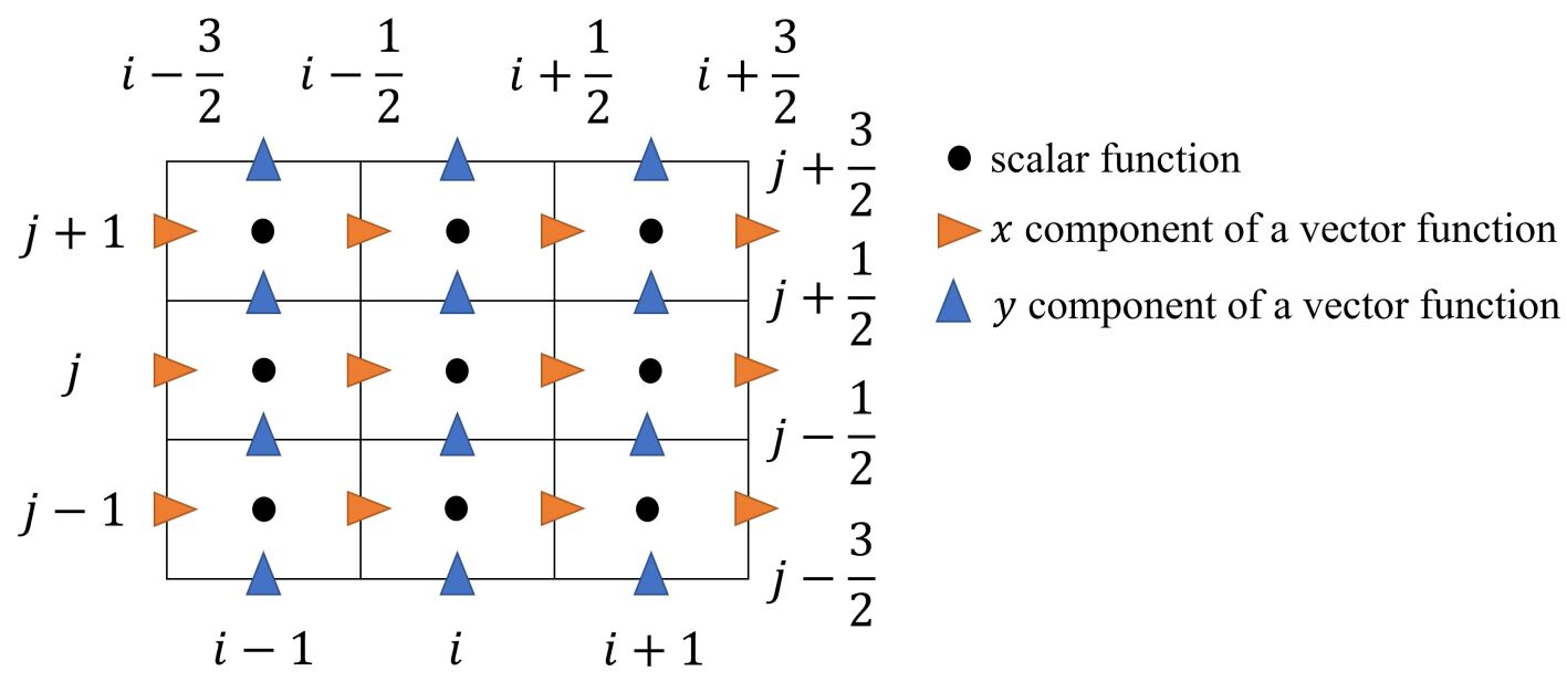
Figure 1: Schematic of the collocated grid. Scalar functions are stored at cell centers. Vector functions are stored at cell faces

The time derivative is approximated by a time discretization scheme denoted by

$$\frac{\partial f}{\partial t}\approx\frac{\gamma_{t}f^{n+1}-\hat{f}}{\Delta t},$$ (35)

where $\gamma_{t}$ and $\hat{(\cdot)}$ are scheme-dependent coefficient and linear operator, respectively, with $\gamma_{t}=\hat{1}$. Notice that Eq.(35) can conceptually represent various time discretization schemes, such as the Runge–Kutta and linear multistep methods.

We denote the linear interpolation along the $x$ axis at $(x_{i},y_{j})$ as

$$\left[\overline{f}^{x}\right]_{i,j}=\frac{1}{2}f_{i-1/2,j}+\frac{1}{2}f_{i+1/2,j}.$$ (36)

The linear interpolation along the other axis can be defined in the same manner. Notice that $\tilde{f}$ can also denote but does not limit to the linear interpolation.

The cell-face gradient is defined at the cell faces and is approximated by the second-order central difference:

$$[\tilde{\nabla}^{x}f]_{i+1/2,j}=\frac{f_{i+1,j}-f_{i,j}}{\Delta x},\quad[\tilde{\nabla}^{y}f]_{i,j+1/2}=\frac{f_{i,j+1}-f_{i,j}}{\Delta y},$$ (37)

where $f$ is a scalar function defined at the cell centers. As a result, $\tilde{\nabla}f$ is a vector function defined at the cell faces. The cell-center gradient is linearly interpolated from the cell-face gradient:

$$\left[\overline{\tilde{\nabla}f}\right]_{i,j}=\left(\left[\overline{\tilde{\nabla}^{x}f}^{x}\right]_{i,j},\left[\overline{\tilde{\nabla}^{y}f}^{y}\right]_{i,j}\right)$$ (38)

The discrete divergence operator is defined as

$$[\tilde{\nabla}\cdot\mathbf{f}]_{i,j}=\frac{f_{i+1/2,j}^{x}-f_{i-1/2,j}^{x}}{\Delta x}+\frac{f_{i,j+1/2}^{y}-f_{i,j-1/2}^{y}}{\Delta y},$$ (39)

where $\mathbf{f}$ is a vector function defined at the cell faces. For the convection term, i.e., $\mathbf{f}=\mathbf{f}_{1}\widetilde{f_{2}}$, $\mathbf{f}_{1}$ is a vector function defined at the cell faces, and $f_{2}$ is a scalar function defined at the cell centers. For the diffusion term, i.e., $\mathbf{f}=\widetilde{f_{2}}\tilde{\nabla}f_{1}$, both $f_{1}$ and $f_{2}$ are scalar functions defined at the cell centers. For the so-called DGT term, i.e., $\mathbf{f}=\widetilde{f_{2}}(\tilde{\nabla}\widetilde{\mathbf{f}_{1}})^{T}$, $\mathbf{f}_{1}$ is a vector function defined at the cell faces and $f_{2}$ is a scalar function defined at the cell centers. A special interpolation to compute $\widetilde{\mathbf{f}_{1}}$ in the DGT term is developed in (Huangetal2020, ) so that $\tilde{\nabla}\cdot(\tilde{\nabla}\widetilde{\mathbf{f}_{1}})^{T}=\overline{\tilde{\nabla}(\tilde{\nabla}\cdot\mathbf{f}_{1})}$ is true. We refer interested readers to (Huangetal2020, ) for detailed definitions of all the discrete operators and for treatments of boundary conditions.

In the present study, a discrete differential operator is called conservative if its summation over all its nodal points is zero in a periodic domain. Conservative operators help to achieve mass and momentum conservation.

Lemma 3.1.

The discrete gradient and divergence operators defined in Eq.(37), Eq.(38), and Eq.(39) are conservative, i.e.,

$$\sum_{i,j}[\tilde{\nabla}^{x}f]_{i+1/2,j}=\sum_{i,j}[\tilde{\nabla}^{y}f]_{i,j+1/2}=0,$$

$$\sum_{i,j}\left[f_{2}\overline{\left(\frac{1}{\overline{f_{2}}}\tilde{\nabla}f_{1}\right)}\right]_{i,j}=\mathbf{0},$$

$$\sum_{i,j}[\tilde{\nabla}\cdot\mathbf{f}]_{i,j}=0.$$

Proof.

For the gradient operators in Eq.(37) and Eq.(38), we only show their $x$-component, and the procedure is the same for the other components.

For the cell-face gradient operator in Eq.(37), we have

$$\sum_{i,j}[\tilde{\nabla}^{x}f]_{i+1/2,j}=\sum_{j}\frac{\sum_{i}f_{i+1,j}-\sum_{i}f_{i,j}}{\Delta x}=\sum_{j}\frac{\sum_{i}f_{i,j}-\sum_{i}f_{i,j}}{\Delta x}=\sum_{j}0=0.$$

For the cell-center gradient operator in Eq.(38), using the definition of the linear interpolation in Eq.(36), we have

$$\sum_{i,j}\left[f_{2}\overline{\left(\frac{1}{\overline{f_{2}}^{x}}\tilde{\nabla}^{x}f_{1}\right)}^{x}\right]_{i,j}=\sum_{i,j}\left(\frac{[f_{2}]_{i,j}}{2}\left[\frac{1}{\overline{f_{2}}^{x}}\tilde{\nabla}^{x}f_{1}\right]_{i-1/2,j}+\frac{[f_{2}]_{i,j}}{2}\left[\frac{1}{\overline{f_{2}}^{x}}\tilde{\nabla}^{x}f_{1}\right]_{i+1/2,j}\right)$$

$$=\sum_{i,j}\frac{[f_{2}]_{i,j}+[f_{2}]_{i+1,j}}{2}\left[\frac{1}{\overline{f_{2}}^{x}}\tilde{\nabla}^{x}f_{1}\right]_{i+1/2,j}=\sum_{i,j}\left[\overline{f_{2}}^{x}\right]_{i+1/2,j}\left[\frac{1}{\overline{f_{2}}^{x}}\tilde{\nabla}^{x}f_{1}\right]_{i+1/2,j}=\sum_{i,j}\left[\tilde{\nabla}^{x}f_{1}\right]_{i+1/2,j}=0.$$

For the divergence operator in Eq.(39), we have

$$\sum_{i,j}[\tilde{\nabla}\cdot\mathbf{f}]_{i,j}=\sum_{j}\frac{\sum_{i}f_{i+1/2,j}^{x}-\sum_{i}f_{i-1/2,j}^{x}}{\Delta x}+\sum_{i}\frac{\sum_{j}f_{i,j+1/2}^{y}-\sum_{j}f_{i,j-1/2}^{y}}{\Delta y}$$

$$=\sum_{j}\frac{\sum_{i}f_{i+1/2,j}^{x}-\sum_{i}f_{i+1/2,j}^{x}}{\Delta x}+\sum_{i}\frac{\sum_{j}f_{i,j+1/2}^{y}-\sum_{j}f_{i,j+1/2}^{y}}{\Delta y}=\sum_{j}0+\sum_{i}0=0.$$

∎

Remark: Lemma 3.1 is true with a zero-gradient boundary condition for the gradient operators and with a zero-flux boundary condition for the divergence operator.

3.2 Gradient-based phase selection procedure

On the continuous level, the convection term in the Phase-Field equation Eq.(7) has the following two properties: (i) $\sum_{p=1}^{N}\nabla\cdot(\mathbf{u}\phi_{p})=(2-N)\nabla\cdot\mathbf{u}$ and (ii) $\nabla\cdot(\mathbf{u}\phi_{p})=-\nabla\cdot\mathbf{u}$ provided $\phi_{p}=-1$ and $\nabla\phi_{p}=\mathbf{0}$. We discover that the discrete convection term can produce fictitious phases, local voids, or overfilling, due to violating the two properties above, which has not been realized in previous studies. The gradient-based phase selection procedure is developed to address those unphsyical behaviors.

The discrete convection term is denoted by $\{\tilde{\nabla}\cdot(\mathbf{u}\widetilde{\phi_{p}})\}_{p=1}^{N}$, where $\mathbf{u}$ is the cell-face velocity and $\tilde{\phi}$ represents interpolated values at the cell-faces from the nodal values of $\phi$ at the cell centers. The gradient-based phase selection procedure has the following steps at each cell face:

• Step 1: compute the convection fluxes $\{\mathbf{u}\widetilde{\phi_{p}}\}_{p=1}^{N}$ with any interpolation method, linear or non-linear,

• Step 2: compute the normal gradients of the order parameters, i.e., $\{\tilde{\nabla}^{n}\phi_{p}\}_{p=1}^{N}=\{\tilde{\nabla}^{x}\phi_{p}\}_{p=1}^{N}$ at $(x_{i+1/2},y_{j})$ and $\{\tilde{\nabla}^{n}\phi_{p}\}_{p=1}^{N}=\{\tilde{\nabla}^{y}\phi_{p}\}_{p=1}^{N}$ at $(x_{i},y_{j+1/2})$,

• Step 3: specify Phase $q$ such that $|\tilde{\nabla}^{n}\phi_{q}|$ is maximum among all the phases,

• Step 4: correct the convection flux of Phase $q$ using

  $$\mathbf{u}\widetilde{\phi_{q}}=(2-N)\mathbf{u}-\sum_{p=1,p\neq q}^{N}\mathbf{u}\widetilde{\phi_{p}}.$$

Then, one can compute the discrete convection term $\{\tilde{\nabla}\cdot(\mathbf{u}\widetilde{\phi_{p}})\}_{p=1}^{N}$ at all the cell centers. After implementing the gradient-based phase selection procedure, it is obvious that the discrete convection term satisfies property (i), i.e., $\sum_{p=1}^{N}\{\tilde{\nabla}\cdot(\mathbf{u}\widetilde{\phi_{p}})\}_{p=1}^{N}=(2-N)\tilde{\nabla}\cdot\mathbf{u}$. Suppose $\phi_{p}=-1$ in the stencil of the interpolation, therefore, we have $\widetilde{\phi_{p}}=-1$ and $\tilde{\nabla}^{n}\phi_{p}=0$. As a result, Phase $p$ will not be selected in Step 3 to perform the correction in Step 4, and we achieve $\tilde{\nabla}\cdot(\mathbf{u}\widetilde{\phi_{p}})=-\tilde{\nabla}\cdot\mathbf{u}$, which is property (ii). The gradient-based phase selection procedure may also improve the robustness and accuracy of the discrete convection term because it corrects the interpolation of the order parameter having the largest local gradient. Usually, interpolation methods are less accurate and may produce oscillations where the gradient is large. It is worth mentioning that the gradient-based phase selection procedure works in any interpolation method to obtain $\{\widetilde{\phi_{p}}\}_{p=1}^{N}$ at the cell faces. Since the convection term is treated explicitly in the present study, the CFL condition is a suitable guidance for numerical stability. Rigorous analyses of the effect of the gradient-based phase selection procedure on numerical stability are difficult, but our numerical test in Section 5.1.4 indicates that using a CFL number of $0.1$ is able to successfully solve an advection problem with a maximum density ratio of $10^{9}$. Implicit treatments to the convection term with the gradient-based phase selection procedure are possible but involved in practice.

Without implementing the gradient-based phase selection procedure, there is nothing to guarantee that $\sum_{p=1}^{N}\widetilde{\phi_{p}}=(2-N)$, see Eq.(4), even though $\sum_{p=1}^{N}\phi_{p}=(2-N)$ is true at every cell center, because the summation and interpolation may not be interchangeable, especially when the interpolation is non-linear. Failure of satisfying $\sum_{p=1}^{N}\tilde{\nabla}\cdot(\mathbf{u}\widetilde{\phi_{p}})=(2-N)\tilde{\nabla}\cdot\mathbf{u}$ results in the same failure of $\sum_{p=1}^{N}\phi_{p}=(2-N)$, see the proof of Theorem 4.2 and the numerical studies in Section 5.1.5.

In many previous studies, e.g., in (LeeKim2015, ; KimLee2017, ; Dong2014, ; Dong2018, ), only the first $(N-1)$ phases are numerically solved from their Phase-Field equation, and the last phase is obtained algebraically from their summation, i.e., Eq.(4). This is equivalent to always correcting the convection flux of Phase $N$. Such a strategy can violate the consistency of reduction and, as a result, generate fictitious phases. Suppose Phase $N$ is absent, i.e., $\phi_{N}\equiv-1$, we have $\sum_{p=1}^{N-1}\phi_{p}=(3-N)$ from Eq.(4). However, this is not guaranteed after the interpolation since $\{\widetilde{\phi_{p}}\}_{p=1}^{N-1}$ are computed independently. The discrete convection flux of Phase $N$ now is $\left[(2-N)\tilde{\nabla}\cdot\mathbf{u}-\sum_{p=1}^{N-1}\tilde{\nabla}\cdot(\mathbf{u}\widetilde{\phi_{p}})\right]=\tilde{\nabla}\cdot\left((2-N-\sum_{p=1}^{N-1}\widetilde{\phi_{p}})\mathbf{u}\right)$ and may not be $-\tilde{\nabla}\cdot\mathbf{u}$. As a result, the convection term becomes a numerical source to produce Phase $N$. Therefore, the phase selection in Step 3 is essential to preserve the consistency of reduction, see the proof of Theorem 4.1 and the numerical studies in Section 5.1.5.

3.3 Discretization of the surface force

In this section, we consider the discretization of the surface force $\mathbf{f}_{s}$ defined in Eq.(23). Under the hydrostatic case, i.e., $\mathbf{u}\equiv\mathbf{0}$, the net force acting on the fluid mixture, i.e., the summation of the pressure gradient, the gravity, and the surface force, should be zero, from the momentum equation Eq.(15). The discretization of the surface force should reproduce this property on the discrete level as much as possible to avoid the spurious currents due to numerical force imbalance. We use $\mathbf{G}$ to denote the discretized net force per unit mass and $\mathbf{G}_{s}$ is the net force per unit mass excluding the pressure gradient, i.e.,

$$\mathbf{G}=-\frac{1}{\overline{\rho}}\tilde{\nabla}P+\mathbf{G}_{s},\quad\mathbf{G}_{s}=\frac{1}{\overline{\rho}}\mathbf{f}_{s}+\mathbf{g},$$ (40)

As defined in Section 3.1, the discrete gradient operator is first computed at the cell faces and then interpolated to the cell centers, see Eq.(37) and Eq.(38). In order to achieve a good numerical balance between the surface force and the pressure gradient, the surface force should follow the same procedure, as pointed out in (Francoisetal2006, ).

In the following, we first introduce the balanced-force method, which is directly extended from its two-phase counterpart, and then develop a novel method, called the conservative method, which helps to conserve the momentum on the discrete level. To avoid repeated algebra, we focus on only the $x$-component of the surface force, and the other components are computed following the same manner. We will further numerically study the performances of these two methods on discrete force balance, see Section 5.1.2, and on discrete momentum conservation, see Section 5.1.5, in the multiphase flow problems.

3.3.1 The balanced-force method

The balanced-force method for the surface force in Eq.(23) reads

$$[f_{s}^{x}]_{i+1/2,j}=\frac{1}{2}\sum_{p=1}^{N}\left[\overline{\xi_{p}}^{x}\right]_{i+1/2,j}[\tilde{\nabla}^{x}\phi_{p}]_{i+1/2,j}.$$ (41)

The balanced-force method is directly extended from the one for the two-phase flows, e.g., in (Francoisetal2006, ; Huangetal2020, ), because the surface force in Eq.(23) has a form of a scalar times the gradient of another scalar, the same structure as the two-phase surface tension models, e.g., in (Brackbilletal1992, ; Sussmanetal1994, ; Jacqmin1999, ). The two-phase balanced-force method has been extensively studied and popularly used, e.g., in (Francoisetal2006, ; Huangetal2020, ; Huangetal2020CAC, ; Mirjalili2019, ).

3.3.2 The conservative method

The newly developed conservative method discretizes the following equivalent form of the surface force in Eq.(23), i.e.,

$$\mathbf{f}_{s}=\frac{1}{2}\sum_{p=1}^{N}\xi_{p}\nabla\phi_{p}=\frac{1}{2}\sum_{p,q=1}^{N}\lambda_{p,q}\left[\frac{1}{\eta^{2}}\left(g^{\prime}_{1}(\phi_{p})-g^{\prime}_{2}(\phi_{p}+\phi_{q})\right)+\nabla^{2}\phi_{q}\right]\nabla\phi_{p}$$

$$=\frac{1}{2}\sum_{p,q=1}^{N}\lambda_{p,q}\left[\frac{1}{\eta^{2}}\left(\nabla g_{1}(\phi_{p})-\frac{1}{2}\nabla g_{2}(\phi_{p}+\phi_{q})\right)+\nabla^{2}\phi_{q}\nabla\phi_{p}\right],$$

and the conservative method reads

$$[f_{s}^{x}]_{i+1/2,j}=\frac{1}{2}\sum_{p,q=1}^{N}\lambda_{p,q}\left[\frac{1}{\eta^{2}}\left([\tilde{\nabla}^{x}g_{1}(\phi_{p})]_{i+1/2,j}-\frac{1}{2}[\tilde{\nabla}^{x}g_{2}(\phi_{p}+\phi_{q})]_{i+1/2,j}\right)\right.$$ (42)

$$\left.+\left[\overline{\tilde{\nabla}\cdot(\tilde{\nabla}\phi_{q})}^{x}\right]_{i+1/2,j}[\tilde{\nabla}^{x}\phi_{p}]_{i+1/2,j}\right].$$

The conservative method is a general momentum conservative numerical model for interfaceial tensions that can include an arbitrary number of phases. Such a general model has not been developed in previous studies.

Theorem 3.2.

The conservative method Eq.(42) for the surface force in Eq.(23) is conservative, i.e.,

$$\sum_{i,j}[f_{s}^{x}]_{i+1/2,j}=0,\quad\sum_{i,j}[f_{s}^{y}]_{i,j+1/2}=0.$$

Proof.

Following the definition of the gradient operator in Eq.(37), the mixed derivative evaluated at the cell corners is commutable, i.e.,

$$\left[\tilde{\nabla}^{y}(\tilde{\nabla}^{x}\phi)\right]_{i+1/2,j+1/2}=\left[\tilde{\nabla}^{x}(\tilde{\nabla}^{y}\phi)\right]_{i+1/2,j+1/2}.$$

After defining

$$\langle\nabla^{x}\phi_{p}\nabla^{x}\phi_{q}\rangle_{i,j}=\left[\overline{\tilde{\nabla}^{x}\phi_{p}}^{x}\right]_{i,j}\left[\overline{\tilde{\nabla}^{x}\phi_{q}}^{x}\right]_{i,j},$$

$$\langle\nabla^{y}\phi_{p}\nabla^{x}\phi_{q}\rangle_{i+1/2,j+1/2}=\left[\overline{\tilde{\nabla}^{y}\phi_{p}}^{x}\right]_{i+1/2,j+1/2}\left[\overline{\tilde{\nabla}^{x}\phi_{q}}^{y}\right]_{i+1/2,j+1/2},$$

$$\langle\nabla\phi_{p}\cdot\nabla\phi_{q}\rangle_{i,j}=\left[\overline{\tilde{\nabla}^{x}\phi_{p}\tilde{\nabla}^{x}\phi_{q}}^{x}\right]_{i,j}+\left[\overline{\tilde{\nabla}^{y}\phi_{p}\tilde{\nabla}^{y}\phi_{q}}^{y}\right]_{i,j},$$

$$\langle\nabla^{x}\phi_{p}\nabla^{x}(\nabla^{x}\phi_{q})\rangle_{i,j}=\left[\overline{\tilde{\nabla}^{x}\phi_{p}}^{x}\right]_{i,j}[\tilde{\nabla}^{x}(\tilde{\nabla}^{x}\phi_{q})]_{i,j},$$

$$\langle\nabla^{y}\phi_{p}\nabla^{x}(\nabla^{y}\phi_{q})\rangle_{i+1/2,j+1/2}=\left[\overline{\tilde{\nabla}^{y}\phi_{p}}^{x}\right]_{i+1/2,j+1/2}[\tilde{\nabla}^{x}(\tilde{\nabla}^{y}\phi_{q})]_{i+1/2,j+1/2},$$

we obtain the following two identities

$$\left[\overline{\tilde{\nabla}\cdot(\tilde{\nabla}\phi_{p})}^{x}\right]_{i+1/2,j}[\tilde{\nabla}^{x}\phi_{q}]_{i+1/2,j}=\left[\tilde{\nabla}^{x}\langle\nabla^{x}\phi_{p}\nabla^{x}\phi_{q}\rangle\right]_{i+1/2,j}+\left[\tilde{\nabla}^{y}\langle\nabla^{y}\phi_{p}\nabla^{x}\phi_{q}\rangle\right]_{i+1/2,j}$$

$$-\left[\overline{\langle\nabla^{x}\phi_{p}\nabla^{x}(\nabla^{x}\phi_{q})\rangle}^{x}\right]_{i+1/2,j}-\left[\overline{\langle\nabla^{y}\phi_{p}\nabla^{x}(\nabla^{y}\phi_{q})\rangle}^{y}\right]_{i+1/2,j},$$

$$[\tilde{\nabla}^{x}\langle\nabla\phi_{p}\cdot\nabla\phi_{q}\rangle]_{i+1/2,j}=\left[\overline{\langle\nabla^{x}\phi_{p}\nabla^{x}(\nabla^{x}\phi_{q})\rangle}^{x}\right]_{i+1/2,j}+\left[\overline{\langle\nabla^{y}\phi_{p}\nabla^{x}(\nabla^{y}\phi_{q})\rangle}^{y}\right]_{i+1/2,j}$$

$$+\left[\overline{\langle\nabla^{x}\phi_{q}\nabla^{x}(\nabla^{x}\phi_{p})\rangle}^{x}\right]_{i+1/2,j}+\left[\overline{\langle\nabla^{y}\phi_{q}\nabla^{x}(\nabla^{y}\phi_{p})\rangle}^{y}\right]_{i+1/2,j}.$$

Multiplying them with $\lambda_{p,q}$ and summing over $p$ and $q$, we obtain

$$\sum_{p,q=1}^{N}\lambda_{p,q}\left[\overline{\tilde{\nabla}\cdot(\tilde{\nabla}\phi_{q})}^{x}\right]_{i+1/2,j}[\tilde{\nabla}^{x}\phi_{p}]_{i+1/2,j}=\sum_{p,q=1}^{N}\lambda_{p,q}\left[\tilde{\nabla}^{x}\langle\nabla^{x}\phi_{p}\nabla^{x}\phi_{q}\rangle\right]_{i+1/2,j}$$

$$+\sum_{p,q=1}^{N}\lambda_{p,q}\left[\tilde{\nabla}^{y}\langle\nabla^{y}\phi_{p}\nabla^{x}\phi_{q}\rangle\right]_{i+1/2,j}-\frac{1}{2}\sum_{p,q=1}^{N}\lambda_{p,q}[\tilde{\nabla}^{x}\langle\nabla\phi_{p}\cdot\nabla\phi_{q}\rangle]_{i+1/2,j}.$$

Finally, applying Lemma 3.1, we have

$$\sum_{i,j}[f_{s}^{x}]_{i+1/2,j}=0.$$

With the same procedure, we have $\sum_{i,j}[f_{s}^{y}]_{i,j+1/2}=0$. ∎

The difference between the balanced-force method Eq.(41) and the conservative method Eq.(42) is rooted in discretizing $\nabla g_{1}$ and $\nabla g_{2}$. In the conservative method Eq.(42), these two terms are discretized directly using the gradient operators defined in Eq.(37), while in the balanced-force method Eq.(41), the chain rule was applied first and then the gradient operator is applied to $\phi_{p}$ instead. Such a difference between the two methods changes their discrete conservation properties, although the difference is in the order of the truncation error.

3.4 Consistency on the discrete level

In this section, general theorems are newly developed to preserve the consistency conditions on the discrete level, so that the physical coupling between the Phase-Field and momentum equations, discussed in Section 2, is inherited after discretization. Those theorems are on the fully discrete level and independent of the number of phases, the Phase-Field equation, or the scheme to solve the Phase-Field equation, which have not been proposed in previous studies.

Without loss of generality, the fully discrete Phase-Field equation is represented by

$$\frac{\gamma_{t}\phi_{p}^{n+1}-\widehat{\phi_{p}}}{\Delta t}+\tilde{\nabla}\cdot(\mathbf{u}\widetilde{\phi_{p}})=\tilde{\nabla}\cdot\langle\mathbf{J}_{p}\rangle,\quad 1\leqslant p\leqslant N,$$ (43)

where $(\mathbf{u}\widetilde{\phi_{p}})$ and $\langle\mathbf{J}_{p}\rangle$ are the discrete convection and diffusion fluxes, respectively, of Phase $p$. Here, we don’t need to know how $\langle\mathbf{J}_{p}\rangle$ is defined or computed. The time discretization scheme (denoted by $\gamma_{t}$ and $\hat{(\cdot)}$), the discrete divergence operator (denoted by $\tilde{\nabla}\cdot(\cdot)$), and the interpolation (denoted by $\tilde{\phi}$) can be arbitrary. We only assume that Eq.(43) follows the consistency of reduction, and therefore $\{\langle\mathbf{J}_{p}\rangle\}_{p=1}^{N}$ meet the requirements in Theorem 2.1. To simplify the notation, we define the discrete Phase-Field flux of Phase $p$ as $\langle\mathbf{m}_{\phi_{p}}\rangle=\mathbf{u}\widetilde{\phi_{p}}-\langle\mathbf{J}_{p}\rangle$.

3.4.1 The consistency of mass conservation on the discrete level

The following theorem guarantees the consistency of mass conservation on the discrete level.

Theorem 3.3.

Given the discrete Phase-Field fluxes $\{\langle\mathbf{m}_{\phi_{p}}\rangle\}_{p=1}^{N}$ that satisfy the fully discrete Phase-Field equation, i.e.,

$$\frac{\gamma_{t}\phi_{p}^{n+1}-\widehat{\phi_{p}}}{\Delta t}+\tilde{\nabla}\cdot\langle\mathbf{m}_{\phi_{p}}\rangle=0,\quad 1\leqslant p\leqslant N,$$

and provided a cell-face velocity $\mathbf{u}$ that is discretely divergence-free, i.e.,

$$\tilde{\nabla}\cdot\mathbf{u}=0,$$

the corresponding discrete consistent mass flux that satisfies the consistency of mass conservation on the discrete level is

$$\langle\mathbf{m}\rangle=\sum_{p=1}^{N}\frac{\rho_{p}}{2}(\mathbf{u}+\langle\mathbf{m}_{\phi_{p}}\rangle),$$ (44)

which results in the fully discrete mass conservation equation

$$\frac{\gamma_{t}\rho^{n+1}-\hat{\rho}}{\Delta t}+\tilde{\nabla}\cdot\langle\mathbf{m}\rangle=0.$$ (45)

It should be noted that $\gamma_{t}$, $\hat{(\cdot)}$, and $\tilde{\nabla}\cdot(\cdot)$ in the fully discrete mass conservation equation are identical to those in the fully discrete Phase-Field equation.

Proof.

Using Eq.(5) for $\rho$, Eq.(44) for $\langle\mathbf{m}\rangle$, and $\gamma_{t}$, $\hat{(\cdot)}$, and $\tilde{\nabla}\cdot(\cdot)$ in the fully discrete Phase-Field equation, we have

$$\frac{\gamma_{t}\rho^{n+1}-\hat{\rho}}{\Delta t}+\tilde{\nabla}\cdot\langle\mathbf{m}\rangle=\sum_{p=1}^{N}\frac{\rho_{p}}{2}\frac{\gamma_{t}(1+\phi_{p}^{n+1})-\widehat{(1+\phi_{p})}}{\Delta t}+\tilde{\nabla}\cdot\sum_{p=1}^{N}\frac{\rho_{p}}{2}(\mathbf{u}+\langle\mathbf{m}_{\phi_{p}}\rangle)$$

$$=\sum_{p=1}^{N}\frac{\rho_{p}}{2}\left(\frac{\gamma_{t}-\overbrace{\hat{1}}^{\gamma_{t}}}{\Delta t}+\underbrace{\tilde{\nabla}\cdot\mathbf{u}}_{0}\right)+\sum_{p=1}^{N}\frac{\rho_{p}}{2}\underbrace{\left(\frac{\gamma_{t}\phi_{p}^{n+1}-\widehat{\phi_{p}}}{\Delta t}+\tilde{\nabla}\cdot\langle\mathbf{m}_{\phi_{p}}\rangle\right)}_{0}=0.$$

Therefore, the consistency of mass conservation is satisfied on the discrete level, and $\langle\mathbf{m}\rangle$ in Eq.(44) is the discrete consistent mass flux. ∎

3.4.2 The consistency of mass and momentum transport on the discrete level

The consistency of mass and momentum transport on the discrete level can be formulated in the following theorem:

Theorem 3.4.

Given the discrete consistent mass flux $\langle\mathbf{m}\rangle$ that satisfies the consistency of mass conservation, i.e., the fully discrete mass conservation equation is

$$\frac{\gamma_{t}\rho^{n+1}-\hat{\rho}}{\Delta t}+\tilde{\nabla}\cdot\langle\mathbf{m}\rangle=0,$$

to satisfy the consistency of mass and momentum transport on the discrete level, the momentum equation Eq.(15) is discretized as

$$\frac{\gamma_{t}\rho^{n+1}\mathbf{u}^{n+1}-\widehat{(\rho\mathbf{u})}}{\Delta t}+\tilde{\nabla}\cdot(\langle\mathbf{m}\rangle\otimes\tilde{\mathbf{u}})=\langle\mathbf{f}\rangle,$$

where $\tilde{\mathbf{u}}$ represents an interpolation of $\mathbf{u}$ to the cell faces, and for simplicity $\langle\mathbf{f}\rangle$ denotes the discretized right-hand side of the momentum equation Eq.(15). It should be noted that $\gamma_{t}$, $\hat{(\cdot)}$, $\tilde{\nabla}\cdot(\cdot)$, and $\langle\mathbf{m}\rangle$ in the discretized momentum equation are identical to those in the fully discrete mass conservation equation.

Corollary 3.4.1.

The discrete momentum transport, i.e.,

$$\frac{\gamma_{t}\rho^{n+1}\mathbf{u}^{n+1}-\widehat{(\rho\mathbf{u})}}{\Delta t}+\tilde{\nabla}\cdot(\langle\mathbf{m}\rangle\otimes\tilde{\mathbf{u}})=\mathbf{0},$$

admits an arbitrary homogeneous velocity as the solution.

Proof.

The discrete momentum transport with a homogeneous velocity $\mathbf{u}_{0}$ becomes

$$\mathbf{u}_{0}\left(\frac{\gamma_{t}\rho^{n+1}-\hat{\rho}}{\Delta t}+\tilde{\nabla}\cdot\langle\mathbf{m}\rangle\right)=0.$$

The parentheses group the fully discrete mass conservation equation which is zero, and therefore $\mathbf{u}_{0}$ is arbitrary. ∎

Theorem 3.4 follows the definition of the consistency of mass and momentum transport in Section 2.3 but additionally considers the numerical operations in the mass and momentum equations. It is actually the discrete version of the control volume analysis in Section 2.7 but here the control volume is fixed and the differential operators are replaced by their discrete counterparts. If all the forces acting on the fluid mixture is zero, then the fluid mixture has no acceleration. In other words, the velocity of the fluid mixture will not change. This physical configuration is discretely reproduced, as illustrated in Corollary 3.4.1, thanks to satisfying the two consistency conditions on the discrete level.

Remark: From Theorem 3.3 and Theorem 3.4, to achieve the consistency of mass conservation and the consistency of mass and momentum transport on the discrete level simultaneously, the Phase-Field and momentum equations need to be discretized using the same time discretization scheme and discrete divergence operator.

3.4.3 The consistency of reduction on the discrete level

In this section, we consider the consistency of reduction on the discrete level, provided that this consistency condition has been satisfied by the fully discrete Phase-Field equation Eq.(43) as pointed out at the beginning of Section 3.4. Therefore, we in particular focus on the discrete version of the momentum equation Eq.(15) and its related terms, which has seldom been discussed in previous studies.

Without loss of generality, the fully discrete momentum equation can be denoted as

$$\frac{\gamma_{t}\rho^{n+1}\mathbf{u}^{n+1}-\widehat{(\rho\mathbf{u})}}{\Delta t}+\tilde{\nabla}\cdot(\langle\mathbf{m}\rangle\otimes\tilde{\mathbf{u}})=-\langle\nabla P\rangle+\langle\nabla\cdot(\mu\nabla\mathbf{u})\rangle+\langle\nabla\cdot(\mu\nabla\mathbf{u}^{T})\rangle+\langle\rho\mathbf{g}\rangle+\langle\mathbf{f}_{s}\rangle,$$ (46)

where $\langle\cdot\rangle$ represents the discrete mass flux and forces. Again, details of the time discretization scheme, discrete differential operators, interpolations, or computation methods for the mass flux and forces, are not required here.

Theorem 3.5.

If the density and viscosity of the fluid mixture, the discrete consistent mass flux, and the discrete surface force are reduction consistent, then the fully discrete momentum equation Eq.(46) is essentially reduction consistent in the sense that the single-phase case may not be recovered.

Proof.

There is no guarantee that the discrete viscous force $\langle\nabla\cdot(\mu\nabla\mathbf{u})\rangle+\langle\nabla\cdot(\mu\nabla\mathbf{u}^{T})\rangle$ for the multiphase case recovers $\langle\nabla\cdot(\mu\nabla\mathbf{u})\rangle$ for the single-phase case. Therefore, the fully discrete momentum equation Eq.(46) may not be able to recover the sing-phase case, although only the density and viscosity of the fluid mixture, the discrete consistent mass flux, and the discrete surface force are related to the number of phases in Eq.(46) and they are all reduction consistent. ∎

Theorem 3.6.

If the density and viscosity of the fluid mixture, the discrete consistent mass flux, and the discrete surface force are reduction consistent, and $\langle\nabla\cdot(\mu\nabla\mathbf{u}^{T})\rangle$ is exactly zero when $\mu$ is a constant, then the fully discrete momentum equation Eq.(46) is reduction consistent.

Proof.

Continuing the proof of Theorem 3.5 and supplementing the condition that $\langle\nabla\cdot(\mu\nabla\mathbf{u}^{T})\rangle$ becomes zero when $\mu$ is a constant, the fully discrete momentum equation Eq.(46) is able to recover the single-phase case, and therefore is reduction consistent. ∎

Corollary 3.6.1.

If the fully discrete momentum equation Eq.(46) satisfies the consistency of reduction, then it recovers inside each bulk-phase region the corresponding discrete version of the single-phase Navier-Stokes equation with the density and viscosity of that phase, e.g., inside the bulk-phase region of Phase $p$, the fully discrete the momentum equation Eq.(46) becomes

$$\frac{\gamma_{t}\rho_{p}\mathbf{u}^{n+1}-\rho_{p}\widehat{\mathbf{u}}}{\Delta t}+\tilde{\nabla}\cdot\left(\langle\rho_{p}\mathbf{u}\rangle\otimes\tilde{\mathbf{u}}\right)=-\langle\nabla P\rangle+\langle\nabla\cdot(\mu_{p}\nabla\mathbf{u})\rangle+\langle\rho_{p}\mathbf{g}\rangle,$$

which is the fully discrete Navier-Stokes equation with density $\rho_{p}$ and viscosity $\mu_{p}$.

It is obvious that the density and viscosity of the fluid mixture in Eq.(5) and Eq.(6), respectively, meet the requirement in Theorem 3.5 and Theorem 3.6. For the viscous term, we implement the “DGT” operator in (Huangetal2020, ) to discretize $\nabla\cdot(\mu\nabla\mathbf{u}^{T})$, which has the property $\tilde{\nabla}\cdot(\tilde{\nabla}\tilde{\mathbf{u}}^{T})=\overline{\tilde{\nabla}(\tilde{\nabla}\cdot\mathbf{u})}$, as mentioned in Section 3.1. Therefore, as long as the cell-face velocity is discretely divergence-free, the requirement in Theorem 3.6 for the viscous term is satisfied. The remaining task is to analysis the consistency of reduction of the discrete consistent mass flux and the discrete surface force. Following the same argument in Section 2.5, we only need to consider the case where there are $N$ phases ($N\geqslant 2$) and Phase $N$ is absent.

Theorem 3.7.

If the fully discrete Phase-Field equation satisfies the consistency of reduction, and the discretely divergence-free cell-face velocity in Theorem 3.3 is identical to the one in the convection term of the fully discrete Phase-Field equation, then the discrete consistent mass flux in Theorem 3.3 is also reduction consistent.

Proof.

Provided that Phase $N$ is absent, i.e, $\phi_{N}\equiv-1$, and recall that the discrete Phase-Field flux includes both the discrete convection and diffusion fluxes, i.e., $\langle\mathbf{m}_{\phi_{p}}\rangle=\mathbf{u}^{(1)}\widetilde{\phi_{p}}-\langle\mathbf{J}_{p}\rangle$, the discrete consistent mass flux in Theorem 3.3 becomes

$$\langle\mathbf{m}\rangle=\sum_{p=1}^{N}\frac{\rho_{p}}{2}(\mathbf{u}^{(2)}+\langle\mathbf{m}_{\phi_{p}}\rangle)=\sum_{p=1}^{N-1}\frac{\rho_{p}}{2}(\mathbf{u}^{(2)}+\langle\mathbf{m}_{\phi_{p}}\rangle)+\frac{\rho_{N}}{2}(\mathbf{u}^{(2)}+\mathbf{u}^{(1)}\underbrace{\widetilde{\phi_{N}}}_{-1}-\underbrace{\langle\mathbf{J}_{N}\rangle}_{\mathbf{0}})$$

$$=\sum_{p=1}^{N-1}\frac{\rho_{p}}{2}(\mathbf{u}^{(2)}+\langle\mathbf{m}_{\phi_{p}}\rangle)+\frac{\rho_{N}}{2}(\mathbf{u}^{(2)}-\mathbf{u}^{(1)}).$$

Here, $\mathbf{u}^{(1)}$ is the velocity used in the convection term of the fully discrete Phase-Field equation, and $\mathbf{u}^{(2)}$ is the discretely divergence-free cell-face velocity, i.e., $\tilde{\nabla}\cdot\mathbf{u}^{(2)}=0$, in Theorem 3.3. After requiring $\mathbf{u}^{(2)}=\mathbf{u}^{(1)}$, the contribution from Phase $N$ to the discrete consistent mass flux is removed, thanks to the reduction consistent fully discrete Phase-Field equation. As a result, the discrete consistent mass flux in Theorem 3.3 recovers its ($N-1$)-phase formulation excluding the contribution from absent Phase $N$, and therefore it is reduction consistent. ∎

Theorem 3.8.

Both the balanced-force method Eq.(41) and the conservative method Eq.(42) for discretizing the surface force in Eq.(23) are reduction consistent.

Proof.

Provided that Phase $N$ is absent, i.e., $\phi_{N}\equiv-1$, we have $\tilde{\nabla}\phi_{N}=\mathbf{0}$ and $\tilde{\nabla}\cdot(\tilde{\nabla}\phi_{N})=0$. From Eq.(20), we have $g_{1}(\phi)=g_{2}(\phi-1)$, $g^{\prime}_{1}(\phi)=g^{\prime}_{2}(\phi-1)$, and $g_{1}(-1)=0$.

The balanced-force method Eq.(41) becomes

$$\mathbf{f}_{s}=\frac{1}{2}\sum_{p=1}^{N}\overline{\xi_{p}}\tilde{\nabla}\phi_{p}=\frac{1}{2}\sum_{p=1}^{N-1}\overline{\xi_{p}}\tilde{\nabla}\phi_{p},$$

where

$$\xi_{p}=\sum_{q=1}^{N}\lambda_{p,q}\left[\frac{1}{\eta^{2}}\left(g^{\prime}_{1}(\phi_{p})-g^{\prime}_{2}(\phi_{p}+\phi_{q})\right)+\tilde{\nabla}\cdot(\tilde{\nabla}\phi_{q})\right]=\sum_{q=1}^{N-1}\lambda_{p,q}\left[\frac{1}{\eta^{2}}\left(g^{\prime}_{1}(\phi_{p})-g^{\prime}_{2}(\phi_{p}+\phi_{q})\right)+\tilde{\nabla}\cdot(\tilde{\nabla}\phi_{q})\right].$$

The conservative method Eq.(42) becomes

$$\mathbf{f}_{s}=\frac{1}{2}\sum_{p,q=1}^{N}\lambda_{p,q}\left[\frac{1}{\eta^{2}}\left(\tilde{\nabla}g_{1}(\phi_{p})-\frac{1}{2}\tilde{\nabla}g_{2}(\phi_{p}+\phi_{q})\right)+\overline{\tilde{\nabla}\cdot(\tilde{\nabla}\phi_{q})}\tilde{\nabla}\phi_{p}\right]$$

$$=\frac{1}{2}\sum_{p,q=1}^{N-1}\lambda_{p,q}\left[\frac{1}{\eta^{2}}\left(\tilde{\nabla}g_{1}(\phi_{p})-\frac{1}{2}\tilde{\nabla}g_{2}(\phi_{p}+\phi_{q})\right)+\overline{\tilde{\nabla}\cdot(\tilde{\nabla}\phi_{q})}\tilde{\nabla}\phi_{p}\right].$$

As a result, both the balanced-force method Eq.(41) and the conservative method Eq.(42) recovers the corresponding $(N-1)$-phase formulations excluding the contribution from absent Phase $N$, and they therefore are reduction consistent. ∎

Remark:

• Theorem 3.3, Theorem 3.4, and Theorem 3.7 illustrate correspondences of numerical operations in the fully discrete Phase-Field and momentum equations. These correspondences discretely reproduce the physical connection among the Phase-Field equation, the mass conservation, and the momentum transport.

• The issue of the viscous force in the consistency of redaction is totally numerical, and does not appear on the continuous level. An alternative way to meet the requirement in Theorem 3.6 is to first transform $\nabla\cdot(\mu\nabla\mathbf{u}^{T})$ to $\nabla\mu\cdot\nabla\mathbf{u}^{T}$, and then discretize $\nabla\mu\cdot\nabla\mathbf{u}^{T}$. Although this helps to achieve the consistency of reduction, it unfortunately destroys the discrete momentum conservation. On the other hand, the “DGT” operator developed in (Huangetal2020, ) retains the conservative form of the viscous force and helps to achieve the consistency of reduction and at the same time momentum conservation on the discrete level.

4 The consistent and conservative scheme for the present multiphase flow model

In this section, we develop a consistent and conservative scheme specific to the present multiphase flow model including the Phase-Field equation Eq.(7) with the diffusion flux in Eq.(16) and the momentum equation Eq.(15) from the consistency of mass conservation and the consistency of mass and momentum transport. For brevity, in this section, the Phase-Field equation refers to the one with the diffusion flux in Eq.(16).

The present scheme is based on the second-order decoupled scheme in (Dong2018, ) for the Phase-Field equation and the second-order projection scheme in (Huangetal2020, ) for the momentum equation, but implements the novel numerical techniques developed in Section 3 to satisfy all the consistency conditions, to achieve mass and momentum conservation, and to assure the summation of the volume fractions to be unity (or Eq.(4)), on the discrete level. Analyses of those properties of the scheme are performed, which were not reported in (Dong2018, ; Huangetal2020, ). Hereafter, the time discretization scheme is the second-order backward difference, i.e., $\gamma_{t}=1.5$ and $\hat{f}=2f^{n}-0.5f^{n-1}$, and the second-order $f^{*,n+1}$ is $(2f^{n}-f^{n-1})$. The discrete differential operators defined in Section 3.1 are used. This ensures that the same time discretization scheme and discrete divergence operator will be used to discretize the Phase-Field and momentum equations, which is critical to achieve the consistency of mass conservation and the consistency of mass and momentum transport on the discrete level, see Theorem 3.3 and Theorem 3.4. The interpolation denoted by $\tilde{f}$ for example is specific to the 5th-order WENO scheme (JiangShu1996, ) here.

4.1 Scheme for the Phase-Field equation

The Phase-Field equation is solved by the following two steps.

Step 1: Solve for $\{\psi_{p}^{n+1}\}_{p=1}^{N}$ from

$$\tilde{\nabla}\cdot(\tilde{\nabla}\psi_{p}^{n+1})-(\alpha+S)\psi_{p}^{n+1}=\left[\tilde{\nabla}\cdot(\tilde{\nabla}\psi_{p}^{*,n+1})-(\alpha+S)\tilde{\nabla}\cdot(\tilde{\nabla}\phi_{p}^{*,n+1})\right]$$ (47)

$$+\frac{1}{\gamma_{0}}\left[\frac{\widehat{\phi_{p}}}{\Delta t}-\tilde{\nabla}\cdot\left(\mathbf{u}^{*,n+1}\widetilde{\phi_{p}^{*,n+1}}\right)+\sum_{q=1}^{N}\tilde{\nabla}\cdot\left(\overline{M_{p,q}^{*,n+1}}\tilde{\nabla}\xi_{q}^{*,n+1}\right)\right],\quad 1\leqslant p\leqslant N.$$

Step 2: Solve for $\{\phi_{p}^{n+1}\}_{p=1}^{N}$ from

$$\tilde{\nabla}\cdot(\tilde{\nabla}\phi_{p}^{n+1})+\alpha\phi_{p}^{n+1}=\psi_{p}^{n+1},\quad 1\leqslant p\leqslant N.$$ (48)

Here, $\alpha$ satisfies

$$\alpha^{2}+S\alpha+\frac{\gamma_{t}}{\gamma_{0}\Delta t}=0,$$ (49)

or explicitly, $\alpha=\frac{1}{2}\left[-S+\sqrt{S^{2}-\frac{4\gamma_{t}}{\gamma_{0}\Delta t}}\right]$ with $S\geqslant\sqrt{\frac{4\gamma_{t}}{\gamma_{0}\Delta t}}$, and $\gamma_{0}=NM_{0}\sum_{p,q=1}^{N}\lambda_{p,q}$.

The boundary conditions, unless otherwise specified, for $\{\phi_{p}^{n+1}\}_{p=1}^{N}$ and $\{\psi_{p}^{n+1}\}_{p=1}^{N}$ are, respectively,

$$\mathbf{n}\cdot\tilde{\nabla}\phi_{p}^{n+1}=\sum_{q=1}^{N}\zeta_{p,q}\frac{1+\phi_{p}^{*,n+1}}{2}\frac{1+\phi_{q}^{*,n+1}}{2},\quad 1\leqslant p\leqslant N,$$ (50)

$$\mathbf{n}\cdot\tilde{\nabla}\psi_{p}^{n+1}=\mathbf{n}\cdot\tilde{\nabla}\left[\psi_{p}^{*,n+1}+(\alpha+S)(\phi_{p}^{n+1}-\phi_{p}^{*,n+1})\right]+\frac{1}{\gamma_{0}}\sum_{q=1}^{N}\mathbf{n}\cdot\left(\overline{M_{p,q}^{*,n+1}}\tilde{\nabla}\xi_{q}^{*,n+1}\right),\quad 1\leqslant p\leqslant N,$$ (51)

where $\mathbf{n}$ is the unit outward normal at the domain boundary, and $\zeta_{p,q}$ is defined in Eq.(25).

This scheme for the Phase-Field equation was originated in (Dong2018, ) and several modifications have been performed in the present study to eliminate unphysical results. (i) To conserve the order parameters and therefore the mass of each phase, the convection term is computed from its conservative form, i.e., $\nabla\cdot(\mathbf{u}\phi)$, while in (Dong2018, ) it is computed from its non-conservative form, i.e., $\mathbf{u}\cdot\nabla\phi$. (ii) To satisfy the consistency of reduction, all the order parameters are solved from the scheme, i.e., Eq.(47) and Eq.(48), while in (Dong2018, ) only the first $(N-1)$ order parameters are solved from the scheme and the last one is obtained algebraically from their summation, i.e., Eq.(4). As discussed in Section 3.2, such an implementation in (Dong2018, ) can easily violate the consistency of reduction and produce fictitious phases numerically. (iii) To additionally satisfy the summation of the order parameters, the gradient-based phase selection procedure, developed in Section 3.2, has been implemented to the convection terms $\left\{\tilde{\nabla}\cdot\left(\mathbf{u}^{*,n+1}\widetilde{\phi_{p}^{*,n+1}}\right)\right\}_{p=1}^{N}$ in Eq.(47).

In summary, the present scheme for the Phase-Field equation including the newly proposed gradient-based phase selection procedure in Section 3.2 has the following provable properties on the discrete level:

• It satisfies the consistency of reduction, see Theorem 4.1, and therefore no fictitious phases can be numerically produced.

• It satisfies the summation of the order parameters, see Theorem 4.2, and therefore no local voids or overfilling can be numerically produced.

• It conserves the order parameters and therefore the mass of each phase and the mass of the fluid mixture, see Theorem 4.3.

4.1.1 Properties of the scheme for the Phase-Field equation

Here, we analyze the physical properties of the scheme for the Phase-Field equation and illustrate the significance of including the gradient-based phase selection procedure in Section 3.2. It should be noted that the following analyses were not available in (Dong2018, ) where the scheme was originated.

The corresponding fully discrete Phase-Field equation of the scheme is

$$\frac{\gamma_{t}\phi_{p}^{n+1}-\widehat{\phi_{p}}}{\Delta t}+\tilde{\nabla}\cdot\left(\mathbf{u}^{*,n+1}\widetilde{\phi_{p}^{*,n+1}}\right)=\tilde{\nabla}\cdot\langle\mathbf{J}_{p}\rangle,$$ (52)

$$\langle\mathbf{J}_{p}\rangle=\sum_{q=1}^{N}\overline{M_{p,q}^{*,n+1}}\tilde{\nabla}\xi_{q}^{*,n+1}-\gamma_{0}\tilde{\nabla}\left[(\psi_{p}^{n+1}-\psi_{p}^{*,n+1})-(\alpha+S)(\phi_{p}^{n+1}-\phi_{p}^{*,n+1})\right].$$

Compared to its continuous correspondence Eq.(16), the last term in the discrete diffusion flux $\langle\mathbf{J}_{p}\rangle$ is newly introduced. It comes from decoupling the Phase-Field equation among the fluid phases and is zero on the continuous level. Since the time derivative is approximated by the second-order backward difference and the difference between $(\cdot)^{*,n+1}$ and $(\cdot)^{n+1}$ is $O(\Delta t^{2})$, the scheme is formally second-order accurate in time. As one shall see in Section 4.3, the cell-face velocity is discretely divergence-free at all the time level (Eq.(62)), and therefore $\tilde{\nabla}\cdot\mathbf{u}^{*,n+1}=\tilde{\nabla}\cdot(2\mathbf{u}^{n}-\mathbf{u}^{n-1})=(2\tilde{\nabla}\cdot\mathbf{u}^{n}-\tilde{\nabla}\cdot\mathbf{u}^{n-1})=(\tilde{\nabla}\cdot\mathbf{u})^{*,n+1}=0$. This property will be used in the following analyses.

Theorem 4.1.

The scheme for the Phase-Field equation in Section 4.1 including the gradient-based phase selection procedure in Section 3.2 satisfies the consistency of reduction.

Proof.

Provided that Phase $N$ is absent up time level $n$, i.e., $\phi_{N}^{n},\phi_{N}^{n-1},...,\phi_{N}^{0}\equiv-1$, we first consider the scheme for Phase $N$. The provided condition implies $\phi_{N}^{*,n+1}=-1$, $\widehat{\phi_{N}}=-\gamma_{t}$, $M_{N,q}^{*,n+1}=M_{q,N}^{*,n+1}=0$ from Eq.(17), $\psi_{N}^{*,n+1}=-\alpha$ from Eq.(48), $\tilde{\nabla}\cdot\left(\mathbf{u}^{*,n+1}\widetilde{\phi_{N}^{*,n+1}}\right)=-\tilde{\nabla}\cdot\mathbf{u}^{*,n+1}=0$ thanks to the gradient-based phase selection procedure, see Section 3.2, and to satisfying the divergence-free condition discretely, see Section 4.3. As a result, Eq.(47) for Phase $N$ is

$$\tilde{\nabla}\cdot(\tilde{\nabla}\psi_{N}^{n+1})-(\alpha+S)\psi_{N}^{n+1}=-\frac{\gamma_{t}}{\gamma_{0}\Delta t},$$

and its solution is $\psi_{N}^{n+1}=-\alpha$ after noticing that $\alpha$ satisfies Eq.(49). Using $\psi_{N}^{n+1}=-\alpha$ into Eq.(48), it is obvious that $\phi_{N}^{n+1}=-1$ is the solution. Therefore, Phase $N$, which is absent initially, won’t be generated numerically by the scheme.

Then, we consider the scheme for Phase $p$ $(p\neq N)$. From Eq.(47) and Eq.(48), the only term including other phases is $\sum_{q=1}^{N}\tilde{\nabla}\cdot\left(\overline{M_{p,q}^{*,n+1}}\tilde{\nabla}\xi_{q}^{*,n+1}\right)$, and it becomes $\sum_{q=1}^{N-1}\tilde{\nabla}\cdot\left(\overline{M_{p,q}^{*,n+1}}\tilde{\nabla}\xi_{q}^{*,n+1}\right)$ since $M_{p,N}^{*,n+1}=0$ from Eq.(17). The contribution of absent Phase $N$ to the chemical potential $\{\xi_{p}\}_{p=1}^{N}$ is removed due to $g^{\prime}_{2}(\phi-1)=g^{\prime}_{1}(\phi)$ and $\tilde{\nabla}\cdot(\tilde{\nabla}\phi_{N})=0$, see the definition of the chemical potential in Eq.(18). As a result, the scheme for the present phases recovers the corresponding $(N-1)$-phase formulation excluding the contribution from absent Phase $N$.

Combining the analyses for the absent and present phases, the scheme for the Phase-Field equation including the gradient-based phase selection procedure is reduction consistent. Correspondingly, the fully discrete Phase-Field equation Eq.(52) becomes

$$\frac{\gamma_{t}\phi_{N}^{n+1}-\widehat{\phi_{N}}}{\Delta t}+\underbrace{\tilde{\nabla}\cdot\left(\mathbf{u}^{*,n+1}\widetilde{\phi_{N}^{*,n+1}}\right)}_{0}=\tilde{\nabla}\cdot\underbrace{\langle\mathbf{J}_{N}\rangle}_{\mathbf{0}},$$

$$\frac{\gamma_{t}\phi_{p}^{n+1}-\widehat{\phi_{p}}}{\Delta t}+\tilde{\nabla}\cdot\left(\mathbf{u}^{*,n+1}\widetilde{\phi_{p}^{*,n+1}}\right)=\tilde{\nabla}\cdot\langle\mathbf{J}_{p}\rangle,\quad 1\leqslant p\leqslant(N-1),$$

$$\langle\mathbf{J}_{p}\rangle=\sum_{q=1}^{N-1}\overline{M_{p,q}^{*,n+1}}\tilde{\nabla}\xi_{q}^{*,n+1}-\gamma_{0}\tilde{\nabla}\left[(\psi_{p}^{n+1}-\psi_{p}^{*,n+1})-(\alpha+S)(\phi_{p}^{n+1}-\phi_{p}^{*,n+1})\right],$$

which discretely reproduces Theorem 2.1 and is reduction consistent. ∎

Theorem 4.2.

The scheme for the Phase-Field equation in Section 4.1 including the gradient-based phase selection procedure in Section 3.2 satisfies the summation of the order parameters in Eq.(4).

Proof.

For a clear presentation, we define $\Phi=\sum_{p=1}^{N}\phi_{p}$ and $\Psi=\sum_{p=1}^{N}\psi_{p}$. Provided that $\Phi=(2-N)$ is true up to time level $n$, i.e., $\Phi^{n}=\Phi^{n-1}=...=\Phi^{0}=(2-N)$, we have $\Phi^{*,n+1}=(2-N)$, $\hat{\Phi}=\gamma_{t}(2-N)$, $\Psi^{*,n+1}=\alpha(2-N)$ from Eq.(48), $\sum_{p=1}^{N}\overline{M_{p,q}^{*,n+1}}=\overline{\sum_{p=1}^{N}M_{p,q}^{*,n+1}}=0$ from Eq.(17), and $\sum_{p=1}^{N}\tilde{\nabla}\cdot\left(\mathbf{u}^{*,n+1}\widetilde{\phi_{p}^{*,n+1}}\right)=(2-N)\tilde{\nabla}\cdot\mathbf{u}^{*,n+1}=0$ thanks to the gradient-based phase selection procedure, see Section 3.2, and to satisfying the divergence-free condition discretely, see Section 4.3. Summing Eq.(47) over $p$, we reach the equation for $\Psi^{n+1}$, i.e.,

$$\tilde{\nabla}\cdot(\tilde{\nabla}\Psi^{n+1})-(\alpha+S)\Psi^{n+1}=\frac{\gamma_{t}(2-N)}{\gamma_{0}\Delta t},$$

and $\Psi^{n+1}=\alpha(2-N)$ is the solution after noticing that $\alpha$ satisfies Eq.(49). The equation for $\Phi$ is obtained by summing Eq.(48) over $p$, i.e.,

$$\tilde{\nabla}\cdot(\tilde{\nabla}\Phi^{n+1})+\alpha\Phi^{n+1}=\Psi^{n+1},$$

and the solution of $\Phi^{n+1}$ is $(2-N)$ after using $\Psi^{n+1}=\alpha(2-N)$.

As a result, we have $\Phi^{n+1}=\sum_{p=1}^{N}\phi_{p}=(2-N)$, as well as the summation of the volume fractions to be unity, i.e., $\sum_{p=1}^{N}C_{p}^{n+1}=\sum_{p=1}^{N}\frac{1+\phi_{p}^{n+1}}{2}=1$, at every cell center. ∎

Remark: The novel gradient-based phase selection procedure in Section 3.2 is essential in the proofs of Theorem 4.1 and Theorem 4.2. Without performing this procedure, the convection term will not become zero for the absent phases or after summing over all the phases, but acts as a numerical source to generate fictitious phases, local voids, or overfilling. These unphysical behaviors are observed in the numerical tests in Section 5.1.5 when the gradient-based phase selection procedure is deactivated.

Theorem 4.3.

The scheme for the Phase-Field equation in Section 4.1 including the gradient-based phase selection procedure in Section 3.2 conserves the order parameters, and therefore the mass of each phase and the mass of the fluid mixture, i.e.,

$$\sum_{i,j}[\phi_{p}^{n}]_{i,j}\Delta\Omega=\sum_{i,j}[\phi_{p}^{0}]_{i,j}\Delta\Omega,\quad[\mathrm{Mass}]_{p}^{n}=[\mathrm{Mass}]_{p}^{0},\quad 1\leqslant p\leqslant N,\quad\mathrm{and}\quad[\mathrm{Mass}]^{n}=[\mathrm{Mass}]^{0},$$

where $[\mathrm{Mass}]_{p}^{n}=\sum_{i,j}\left[\rho_{p}\frac{1+\phi_{p}^{n}}{2}\right]_{i,j}\Delta\Omega$ and $[\mathrm{Mass}]^{n}=\sum_{i,j}[\rho^{n}]_{i,j}\Delta\Omega$.

Proof.

Given $\sum_{i,j}[\phi_{p}^{n}]_{i,j}=\sum_{i,j}[\phi_{p}^{n-1}]_{i,j}=...=\sum_{i,j}[\phi_{p}^{0}]_{i,j}$, we have $\sum_{i,j}[\widehat{\phi_{p}}]_{i,j}=\widehat{\sum_{i,j}[\phi_{p}]_{i,j}}=\gamma_{t}\sum_{i,j}[\phi_{p}^{0}]_{i,j}$. Summing the fully discrete Phase-Field equation Eq.(52) over all the cells and applying Lemma 3.1, we reach

$$\sum_{i,j}[\phi_{p}^{n+1}]_{i,j}=\frac{1}{\gamma_{t}}\sum_{i,j}[\widehat{\phi_{p}}]_{i,j}=\sum_{i,j}[\phi_{p}^{0}]_{i,j},\quad 1\leqslant p\leqslant N.$$

As a result, $\sum_{i,j}[\phi_{p}]_{i,j}\Delta\Omega$ and $[\mathrm{Mass}]_{p}=\sum_{i,j}\left[\rho_{p}\frac{1+\phi_{p}}{2}\right]_{i,j}\Delta\Omega$ ($1\leqslant p\leqslant N$) will not change as time advances. From Eq.(5), we have $[\mathrm{Mass}]=\sum_{p=1}^{N}[\mathrm{Mass}]_{p}$, and therefore $[\mathrm{Mass}]$ will not change as time advances. ∎

4.2 The discrete consistent mass flux

To obtain the discrete consistent mass flux after solving the Phase-Field equation with the scheme in Section 4.1, we follow Theorem 3.3 and Theorem 3.7 developed in Section 3.4. First from Theorem 3.3, we need to obtain the discrete Phase-Field flux, which includes both the discrete convection and diffusion fluxes, from the fully discrete Phase-Field equation Eq.(52), i.e.,

$$\langle\mathbf{m}_{\phi_{p}}\rangle=\left(\mathbf{u}^{*,n+1}\widetilde{\phi_{p}^{*,n+1}}\right)-\langle\mathbf{J}_{p}\rangle$$ (53)

$$=\left(\mathbf{u}^{*,n+1}\widetilde{\phi_{p}^{*,n+1}}\right)-\sum_{q=1}^{N}\overline{M_{p,q}^{*,n+1}}\tilde{\nabla}\xi_{q}^{*,n+1}$$

$$+\gamma_{0}\tilde{\nabla}\left[(\psi_{p}^{n+1}-\psi_{p}^{*,n+1})-(\alpha+S)(\phi_{p}^{n+1}-\phi_{p}^{*,n+1})\right],$$

$$\quad 1\leqslant p\leqslant N.$$

Then, we need to choose a discretely divergence-free cell-face velocity, and Theorem 3.7 tells that in order to achieve the consistency of reduction on the discrete level, this velocity should be the same as the one in the convection term of the fully discrete Phase-Field equation Eq.(52), which is $\mathbf{u}^{*,n+1}$ in the present case. Notice that $\mathbf{u}^{*,n+1}$ is discretely divergence-free, i.e., $\tilde{\nabla}\cdot\mathbf{u}^{*,n+1}=0$, see Section 4.3. Finally, using the formulation in Theorem 3.3 we obtain the discrete consistent mass flux in the present scheme:

$$\langle\mathbf{m}\rangle=\sum_{p=1}^{N}\frac{\rho_{p}}{2}(\mathbf{u}^{*,n+1}+\langle\mathbf{m}_{\phi_{p}}\rangle).$$ (54)

In summary, the discrete consistent mass flux in the present scheme, i.e., the one in Eq.(54) with the discrete Phase-Field flux in Eq.(53), has the following properties on the discrete level:

• It satisfies the consistency of mass conservation, see Theorem 3.3.

• It satisfies the consistency of reduction, see Theorem 3.7, since the same consistency condition has been satisfied by the fully discrete Phase-Field equation, see Theorem 4.1.

Remark: It should be noted that starting from the continuous formulation of the consistent mass flux in Section 2 and then performing discretization usually fails to obtain the discrete consistent mass flux that satisfies the consistency of mass conservation on the discrete level. The present scheme provides an example that some extra terms, in the order of the truncation error, may appear in the fully discrete Phase-Field equation and therefore in the discrete Phase-Field flux, like the last term in Eq.(53). As a result, directly discretizing the continuous formulation will miss those terms, since they are zero on the continuous level. Moreover, if the numerical operations chosen to discretize the continuous formulation are different from those used in the fully discrete Phase-Field equation, the resulting mass flux will also fail to satisfy the consistency of mass conservation. Therefore, one should follow Theorem 3.3 and Theorem 3.7 developed in Section 3.4, like we did here, to obtain the discrete consistent mass flux.

4.3 Scheme for the momentum equation

The momentum equation Eq.(15) is solved by the following 7 steps.

Step 1: Solve for $\mathbf{u}^{*}$ at the cell centers from

$$\frac{\gamma_{t}\rho^{n+1}\mathbf{u}^{*}-\widehat{(\rho\mathbf{u})}}{\Delta t}+\tilde{\nabla}\cdot(\langle\mathbf{m}\rangle\otimes\widetilde{\mathbf{u}^{*,n+1}})=\rho^{n+1}\overline{\mathbf{G}^{n}}+\tilde{\nabla}\cdot(\overline{\mu^{n+1}}\tilde{\nabla}\mathbf{u}^{*})+\tilde{\nabla}\cdot(\overline{\mu^{n+1}}(\tilde{\nabla}\widetilde{\mathbf{u}^{*,n+1}})^{T}).$$ (55)

Step 2: Solve for $\mathbf{u}^{**}$ at the cell centers from

$$\frac{\gamma_{t}\mathbf{u}^{**}-\gamma_{t}\mathbf{u}^{*}}{\Delta t}=-\overline{\mathbf{G}^{n}}.$$ (56)

Step 3: Solve for $\mathbf{u}^{*}$ at the cell faces from

$$\frac{\gamma_{t}\mathbf{u}^{*}-\gamma_{t}\overline{\mathbf{u}^{**}}}{\Delta t}=-\frac{1}{\overline{\rho^{n+1}}}\tilde{\nabla}P^{n}+\mathbf{G}_{s}^{n+1}.$$ (57)

Step 4: Solve for $P^{\prime}$ at the cell centers from

$$\frac{\gamma_{t}}{\Delta t}(\tilde{\nabla}\cdot\mathbf{u}^{n+1}-\tilde{\nabla}\cdot\mathbf{u}^{*})=-\tilde{\nabla}\cdot\left(\frac{1}{\overline{\rho^{n+1}}}\tilde{\nabla}P^{\prime}\right).$$ (58)

Step 5: Solve for $P^{n+1}$ at the cell centers from

$$P^{n+1}=P^{n}+P^{\prime}.$$ (59)

Step 6: Solve for $\mathbf{u}^{n+1}$ at the cell faces from

$$\frac{\gamma_{t}\mathbf{u}^{n+1}-\gamma_{t}\mathbf{u}^{*}}{\Delta t}=-\frac{1}{\overline{\rho^{n+1}}}\tilde{\nabla}P^{\prime}.$$ (60)

Step 7: Solve for $\mathbf{u}^{n+1}$ at the cell centers from

$$\frac{\gamma_{t}\mathbf{u}^{n+1}-\gamma_{t}\mathbf{u}^{**}}{\Delta t}=\overline{\mathbf{G}^{n+1}}.$$ (61)

The cell-face velocity is required to be discretely divergence-free at all the time level, i.e.,

$$\tilde{\nabla}\cdot\mathbf{u}^{n}=0,\quad n=0,1,2,...$$ (62)

Therefore, $\tilde{\nabla}\cdot\mathbf{u}^{n+1}=0$ is applied in Step 4. In the above steps, $\rho$ and $\mu$ are computed from Eq.(5) and Eq.(6), respectively, at the cell centers. Recall that $\mathbf{G}$ and $\mathbf{G}_{s}$, defined in Eq.(40), are the net force per unit mass and the net force per unite mass excluding the pressure gradient, respectively, when $\mathbf{u}\equiv\mathbf{0}$. To address the odd-even decoupling of the pressure in the collocated grid arrangement, the “Rhie-Chow” interpolation (RhieChow1983, ; FerzigerPeric2002, ; Francoisetal2006, ; Popinet2009, ) has been applied (Step 2 and Step 3). The boundary conditions for velocity and pressure are problem-dependent and will be specified in individual cases in Section 5.

This scheme for the momentum equation Eq.(15) is originated in (Huangetal2020, ) for the two-phase flows. Here, it is applied to the multiphase flows, incorporating with the novel numerical techniques developed in Section 3. Following Theorem 3.4 in Section 3.4, the discrete consistent mass flux $\langle\mathbf{m}\rangle$ obtained from Theorem 3.3 and Theorem 3.7 has been used in the inertia term, in order to achieve the consistency of mass and momentum transport on the discrete level. Following Theorem 3.6 in Section 3.4, we retain the “DGT” operator in (Huangetal2020, ), denoted as $\tilde{\nabla}\cdot(\overline{\mu^{n+1}}(\tilde{\nabla}\widetilde{\mathbf{u}^{*,n+1}})^{T})$ here, so that, along with the discretely divergence-free cell-face velocity, $\tilde{\nabla}\cdot(\tilde{\nabla}\widetilde{\mathbf{u}^{*,n+1}})^{T}=\overline{\tilde{\nabla}(\tilde{\nabla}\cdot\mathbf{u}^{*,n+1})}=\mathbf{0}$ is true, which contributes to the consistency of reduction and momentum conservation on the discrete level. Moreover, the balanced-force method Eq.(41) or the conservative method Eq.(42), developed in Section 3.3, is implemented to compute the surface force in $\mathbf{G}_{s}$ to model multiphase interfacial tensions.

In summary, the present scheme for the momentum equation including the novel numerical techniques in Section 3 has the following properties on the discrete level:

• It satisfies the consistency of mass and momentum transport, see the fully discrete momentum equation Eq.(63) and Theorem 3.4.

• It satisfies the consistency of reduction, see Theorem 3.6, Theorem 3.7, and Theorem 3.8, since the same consistency condition has been satisfied by the fully discrete Phase-Field equation, see Theorem 4.1, and $\tilde{\nabla}\cdot(\tilde{\nabla}\widetilde{\mathbf{u}^{*,n+1}})^{T}$ is zero from the property of the “DGT” operator in (Huangetal2020, ). As a result, the fully discrete momentum equation inside the bulk-phase region of Phase $p$ ($1\leqslant p\leqslant N$) becomes the corresponding fully discrete Navier-Stokes equation

  $$\frac{\gamma_{t}\rho_{p}\mathbf{u}^{n+1}-\rho_{p}\hat{\mathbf{u}}}{\Delta t}+\tilde{\nabla}\cdot(\rho_{p}\mathbf{u}^{*,n+1}\otimes\widetilde{\mathbf{u}^{*,n+1}})=-\overline{\tilde{\nabla}P^{n+1}}+\mu_{p}\tilde{\nabla}\cdot(\tilde{\nabla}\mathbf{u}^{*})+\rho_{p}\mathbf{g},$$

  see the fully discrete momentum equation Eq.(63) and Corollary 3.6.1.

• It solves advection (or translation) problems exactly, independent of the material properties of the fluid phases or the initial shapes of the interfaces, see Theorem 4.4.

• It satisfies the momentum conservation if the surface force is either neglected or computed conservatively, e.g., using the conservative method developed in Section 3.3, see Theorem 4.5 and its corollaries.

• It preserves the kinetic energy transport on the semi-discrete level, i.e., the space is discretized but the time is continuous, with the linear interpolation, see Theorem 4.6.

4.3.1 Properties of the scheme for the momentum equation

Here, we analyze the physical properties of the scheme for the momentum equation Eq.(15) including the novel numerical techniques developed in Section 3. It should be noted that the following analyses were not available in (Huangetal2020, ) where the scheme was originated. The corresponding fully discrete momentum equation of the scheme is

$$\frac{\gamma_{t}\rho^{n+1}\mathbf{u}^{n+1}-\widehat{(\rho\mathbf{u})}}{\Delta t}+\tilde{\nabla}\cdot(\langle\mathbf{m}\rangle\otimes\widetilde{\mathbf{u}^{*,n+1}})=\rho^{n+1}\overline{\left(-\frac{1}{\overline{\rho^{n+1}}}\tilde{\nabla}P^{n+1}+\frac{1}{\overline{\rho^{n+1}}}\mathbf{f}_{s}^{n+1}+\mathbf{g}\right)}$$ (63)

$$+\tilde{\nabla}\cdot(\overline{\mu^{n+1}}\tilde{\nabla}\mathbf{u}^{*})+\tilde{\nabla}\cdot(\overline{\mu^{n+1}}(\tilde{\nabla}\widetilde{\mathbf{u}^{*,n+1}})^{T}).$$

The formal order of accuracy of the scheme is second-order, as analyzed in (Huangetal2020, ).

Theorem 4.4.

Provided that all the forces except the pressure gradient are neglected, the scheme for the momentum equation in Section 4.3 admits any homogeneous velocity and pressure as its solution.

Proof.

Given an initial homogeneous velocity $\mathbf{u}_{0}$ and pressure $P_{0}$, and suppose they are still the solution of the scheme up to time level $n$, we seek for the solution of the scheme at $t^{n+1}$.

From Step 1, the right-hand side of Eq.(55) is zero, since the pressure gradient at $t^{n}$ is zero and the other forces are neglected. As a result, we have

$$\mathbf{u}^{*}=\frac{1}{\rho^{n+1}}\underbrace{\left(\frac{\hat{\rho}-\Delta t\tilde{\nabla}\cdot\langle\mathbf{m}\rangle}{\gamma_{t}}\right)}_{\rho^{n+1}}\mathbf{u}_{0}=\mathbf{u}_{0}.$$

Notice that the terms inside the parentheses are equal to $\rho^{n+1}$ due to satisfying the consistency of mass conservation by the discrete consistent mass flux. From Step 2, we obtain $\mathbf{u}^{**}=\mathbf{u}^{*}=\mathbf{u}_{0}$ and further $\overline{\mathbf{u}^{**}}=\mathbf{u}_{0}$ due to $\overline{\mathbf{G}^{n}}=\mathbf{0}$. From Step 3, we have $\mathbf{u}^{*}$ at the cell faces is again $\mathbf{u}_{0}$, by noticing that both $\tilde{\nabla}P^{n}$ and $\mathbf{G}_{s}^{n+1}$ are zero. From Step 4, we have $\tilde{\nabla}\cdot\mathbf{u}^{*}=\tilde{\nabla}\cdot\mathbf{u}_{0}=0$, and therefore $P^{\prime}$ is a constant. Without loss of generality, we set $P^{\prime}=0$. After that, from Step 5, we have $P^{n+1}=P_{0}$, and from Step 6, $\mathbf{u}^{n+1}$ at the cell faces is $\mathbf{u}_{0}$. Finally from Step 7, $\overline{\mathbf{G}^{n+1}}$ is zero and $\mathbf{u}^{n+1}$ at the cell centers is $\mathbf{u}_{0}$. ∎

Theorem 4.4 is rooted in satisfying the consistency of mass conservation and the consistency of mass and momentum transport. Otherwise, the terms inside the parentheses from Step 1 are not equal to $\rho^{n+1}$ anymore, resulting in $\mathbf{u}^{*}\neq\mathbf{u}_{0}$. This error will be transferred into the upcoming steps of the scheme, leading to a non-homogeneous $P^{\prime}$. As a result, $\mathbf{u}^{n+1}$ is not equal to $\mathbf{u}_{0}$ either. Such unphysical velocity and pressure fluctuations depend on the densities of the phases and probably become a source of numerical instability. A simplified two-phase 1D analysis only considering Step 1 of the scheme are available in our previous work (Huangetal2020, ), where even the pressure gradient is neglected. Theorem 4.4 here is more general since it considers the entire scheme including both the velocity and pressure, and works in mulitphase and multidimensional problems. A comparison study will be performed in Section 5.1.4 to demonstrate Theorem 4.4 and therefore the significance of satisfying the consistency conditions.

Remark:

• Theorem 4.4 corresponds to solving advection (or translation) problems, and it holds independent of the number, the material properties, or the initial shapes of the phases. This is consistent with the physical configuration of the advection problems.

• Theorem 4.4 works when including the viscous force because the viscous force is identically zero with a homogeneous velocity.

• Theorem 4.4 can be extended to the case where the hydrostatic mechanical equilibrium is always satisfied numerically, i.e., $\mathbf{G}\equiv 0$. Recall that $\mathbf{G}$ is the net force per unit mass under $\mathbf{u}\equiv 0$, see its definition in Eq.(40). The initial homogeneous velocity is still the solution of the scheme in this case, and the proof is similar. The only difference is that $P^{\prime}$ can be non-homogeneous. Nonetheless, after combining Step 3 and Step 6, we still have $\mathbf{u}^{n+1}=\overline{\mathbf{u}^{**}}=\mathbf{u}_{0}$ at the cell faces, since $\mathbf{G}^{n+1}$, which is zero, is recovered. This case corresponds to the one in Corollary 3.4.1. It should be noted that $\mathbf{G}\equiv\mathbf{0}$ is seldom achievable in numerical practice.

Theorem 4.5.

If the discrete surface force is conservative, i.e.,

$$\sum_{i,j}[f_{s}^{x}]_{i+1/2,j}=\sum_{i,j}[f_{s}^{y}]_{i,j+1/2}=0,$$

the scheme for the momentum equation in Section 4.3 satisfies the momentum conservation on the discrete level, i.e.,

$$[\mathrm{\mathbf{Momentum}}]^{n}=[\mathrm{\mathbf{Momentum}}]^{0},$$

where $[\mathrm{\mathbf{Momentum}}]^{n}=\sum_{i,j}[\rho^{n}\mathbf{u}^{n}]_{i,j}\Delta\Omega$.

Proof.

Given $\sum_{i,j}[\rho^{n}\mathbf{u}^{n}]_{i,j}=\sum_{i,j}[\rho^{n-1}\mathbf{u}^{n-1}]_{i,j}=...=\sum_{i,j}[\rho^{0}\mathbf{u}^{0}]_{i,j}$, we have $\sum_{i,j}[\widehat{(\rho\mathbf{u})}]_{i,j}=\widehat{\sum_{i,j}[\rho\mathbf{u}]_{i,j}}=\gamma_{t}\sum_{i,j}[\rho^{0}\mathbf{u}^{0}]_{i,j}$. Then, summing the fully discrete momentum equation Eq.(63) over all the cell centers, and using Lemma 3.1, we obtain

$$\frac{\gamma_{t}\sum_{i,j}[\rho^{n+1}\mathbf{u}^{n+1}]_{i,j}-\gamma_{t}\sum_{i,j}[\rho^{0}\mathbf{u}^{0}]_{i,j}}{\Delta t}=\sum_{i,j}\left\{\begin{array}[]{ll}&[f_{s}^{x}]_{i+1/2,j}^{n+1},\quad x-\mathrm{component}\\ &[f_{s}^{y}]_{i,j+1/2}^{n+1},\quad y-\mathrm{component}\\ \end{array}\right.=\mathbf{0}.$$

Notice that the gravity is neglected. As a result, the momentum, i.e., $[\mathrm{\mathbf{Momentum}}]=\sum_{i,j}[\rho\mathbf{u}]_{i,j}\Delta\Omega$, is conserved. ∎

Corollary 4.5.1.

If the surface force in Eq.(23) is computed by the conservative method Eq.(42), the scheme for the momentum equation in Section 4.3 satisfies the momentum conservation on the discrete level.

Corollary 4.5.2.

If the surface force is neglected, the scheme for the momentum equation in Section 4.3 satisfies the momentum conservation on the discrete level.

Corollary 4.5.1 is obvious after noticing Theorem 3.2. On the other hand, when the balanced-force method Eq.(41) is used to compute the surface force in Eq.(23), the momentum is not guaranteed to be conserved on the discrete level. Since the surface force is a local force, which is zero except close to interfaces, and the difference between the balanced-force and conservative methods is in the order of the truncation error, see Section 3.3, it is reasonable to expect that the momentum change introduced by the balanced-force method is small. Effects of the balanced-force method and the conservative method on the momentum conservation will be studied with a numerical experiment in Section 5.1.5.

Theorem 4.6.

The semi-discrete momentum transport of the scheme for the momentum equation in Section 4.3, i.e.,

$$\frac{\partial(\rho\mathbf{u})}{\partial t}+\tilde{\nabla}\cdot(\langle\mathbf{m}\rangle\otimes\widetilde{\mathbf{u}})=\mathbf{0},$$

implies the following semi-discrete kinetic energy transport, i.e.,

$$\frac{\partial e_{K}}{\partial t}+\tilde{\nabla}\cdot\left(\langle\mathbf{m}\rangle\frac{1}{2}\widetilde{(\mathbf{u}\cdot\mathbf{u})}\right)=0,\quad e_{K}=\frac{1}{2}\rho\mathbf{u}\cdot\mathbf{u},$$

$$[\widetilde{(\mathbf{u}\cdot\mathbf{u})}]_{i+1/2,j}=\mathbf{u}_{i,j}\cdot\mathbf{u}_{i+1,j},\quad[\widetilde{(\mathbf{u}\cdot\mathbf{u})}]_{i,j+1/2}=\mathbf{u}_{i,j}\cdot\mathbf{u}_{i,j+1},$$

if $\tilde{\mathbf{u}}$ is computed by the linear interpolation, i.e., $\tilde{\mathbf{u}}=\overline{\mathbf{u}}$.

Proof.

Performing the dot product between $\mathbf{u}$ and the semi-discrete momentum transport, we obtain

$$\frac{\partial e_{K}}{\partial t}+\tilde{\nabla}\cdot\left(\langle\mathbf{m}\rangle\frac{1}{2}\widetilde{(\mathbf{u}\cdot\mathbf{u})}\right)+\frac{\mathbf{u}\cdot\mathbf{u}}{2}\underbrace{\left(\frac{\partial\rho}{\partial t}+\nabla\cdot\langle\mathbf{m}\rangle\right)}_{0}=0.$$

Notice that the semi-discrete mass conservation equation, which is zero, is recovered, thanks to satisfying the consistency of mass conservation by $\langle\mathbf{m}\rangle$. ∎

The second-order backward difference in time, the WENO scheme for the interpolation, and, as demonstrated in (Morinishietal1998, ; Huangetal2020, ), the linearly interpolated pressure gradient, used in the present scheme to solve the momentum equation, are dissipative. After considering Theorem 4.6, it is reasonable to infer that the kinetic energy will decay on the fully discrete level. Analyses of the energy law Eq.(22) on the fully discrete level, which are related to the property of the secondary conservation of the scheme, are very complicated. Thus, we will perform numerical experiments to examine Eq.(22) in Section 5.1.5.

Remark: It is worth mentioning that Theorem 4.4, Theorem 4.5, and Theorem 4.6 in this section do not require a specific form of the discrete mass flux $\langle\mathbf{m}\rangle$. The only requirement on $\langle\mathbf{m}\rangle$ in Theorem 4.4 and Theorem 4.6 is that it satisfies the consistency of mass conservation.

4.4 Summary of the present consistent and conservative scheme

The present consistent and conservative scheme for the multiphase flow model, including the Phase-Field equation Eq.(7) and Eq.(16) and the momentum equation Eq.(15), is performed following the steps below:

1. Implement the gradient-based phase selection procedure in Section 3.2 to compute the convection term in Eq.(47) and then solve for $\{\psi_{p}^{n+1}\}_{p=1}^{N}$ and $\{\phi_{p}^{n+1}\}_{p=1}^{N}$ from Eq.(47) and Eq.(48), respectively.

2. Compute the discrete consistent Phase-Field fluxes $\{\langle\mathbf{m}_{\phi_{p}}\rangle\}_{p=1}^{N}$ from Eq.(53) and then the discrete consistent mass flux from Eq.(44).

3. Compute $\rho^{n+1}$ and $\mu^{n+1}$ from Eq.(5) and Eq.(6), respectively, using $\{\phi_{p}^{n+1}\}_{p=1}^{N}$.

4. Compute $\mathbf{f}_{s}^{n+1}$ from either the balanced-force method Eq.(41) or the conservative method Eq.(42).

5. Solve for $\mathbf{u}^{n+1}$ at both the cell centers and cell faces and $P^{n+1}$ from Eq.(55) to Eq.(61), provided $\tilde{\nabla}\cdot\mathbf{u}^{n+1}=0$, see Eq.(62).

Then, we can proceed to the next time step.

5 Validation and application

In the first part of this section, numerical experiments are performed to validate the present multiphase flow model and scheme. In the second part, realistic multiphase flow problems are performed to demonstrate the capability of the model and scheme.

5.1 Validation

In this section, we investigate the formal order of accuracy, the numerical force balance, and the convergence of the numerical solution of the present multiphase flow model to the sharp-interface solution, and validate the analyses and discussions of the present scheme in Section 4, through numerical experiments. All the setups and results are reported in their dimensionless forms.

5.1.1 Manufactured solution

We perform a manufactured solution problem to validate the formal order of accuracy in both time and space of the present scheme in Section 4. The following source terms

$$S_{\phi_{p}}=\frac{\partial\phi_{p}^{E}}{\partial t}+\nabla\cdot(\mathbf{u}^{E}\phi_{p}^{E})-\sum_{q=1}^{N}\nabla\cdot(M_{p,q}^{E}\nabla\xi_{q}^{E}),\quad 1\leqslant p\leqslant N,$$ (64)

$$\mathbf{S_{u}}=\frac{\partial(\rho^{E}\mathbf{u}^{E})}{\partial t}+\nabla\cdot(\mathbf{m}^{E}\otimes\mathbf{u}^{E})+\nabla p^{E}-\nabla\cdot\left[\mu^{E}(\nabla\mathbf{u}^{E}+(\nabla\mathbf{u}^{E})^{T})\right]-\rho^{E}\mathbf{g}-\mathbf{f}_{s}^{E},$$

are added to the Phase-Field and momentum equations, respectively. Here,

$$\phi_{1}^{E}=\frac{1}{3}\cos(x)\cos(y)\sin(t)-\frac{2}{3},$$ (65)

$$\phi_{2}^{E}=\frac{1}{3}\cos(x)\cos(y)\sin(2t)-\frac{2}{3},$$

$$\phi_{3}^{E}=\frac{1}{3}\cos(x)\cos(y)\sin\left(\frac{1}{2}t\right)-\frac{2}{3},$$

$$\phi_{4}^{E}=-\frac{1}{3}\cos(x)\cos(y)\left[\sin(t)+\sin(2t)+\sin\left(\frac{1}{2}t\right)\right],$$

$$u^{E}=\sin(x)\cos(y)\cos(t),$$

$$v^{E}=-\cos(x)\sin(y)\cos(t),$$

$$P^{E}=\cos(x)\cos(y)\sin(t),$$

are the exact solution of the problem, and $M_{p,q}^{E}$, $\xi_{p}^{E}$, $\rho^{E}$, $\mu^{E}$, $\mathbf{m}^{E}$ and $\mathbf{f}_{s}^{E}$ are computed from their definitions in Section 2 using Eq.(65). Notice that Eq.(65) has already satisfied $\nabla\cdot\mathbf{u}^{E}=0$ and $\sum_{p=1}^{N}\phi_{p}^{E}=(2-N)$.

The domain considered is $[-\pi,\pi]\times[-\pi,\pi]$, and its boundaries are all free-slip, which is consistent with Eq.(65). The material properties and parameters are $\rho_{1}=1$, $\rho_{2}=5$, $\rho_{3}=10$, $\rho_{4}=15$, $\mu_{1}=0.01$, $\mu_{2}=0.02$, $\mu_{3}=0.05$, $\mu_{4}=0.10$, $\sigma_{1,2}=0.01$, $\sigma_{1,3}=0.02$, $\sigma_{1,4}=0.03$, $\sigma_{2,3}=0.04$, $\sigma_{2,4}=0.05$, $\sigma_{3,4}=0.06$, $\mathbf{g}=\{1,-2\}$, $\eta=0.1$, and $M_{0}=0.001$. The initial conditions are obtained from Eq.(65) with $t=0$. We first fix the time step to be $\Delta t=10^{-3}$, and successively refine the cell size $h$ from $2\pi/8$ to $2\pi/128$. The computations are stopped at $t=1$ and we compute the $L_{2}$ error as the root mean square of $f-f^{E}$, and the $L_{\infty}$ error as $\mathrm{max}|f-f^{E}|$, where $f$ is the variable of interest and $f^{E}$ is its exact value.

Table 1 lists results obtained by using the balanced-force method Eq.(41). We observe second-order convergences of both the $L_{2}$ and $L_{\infty}$ errors for all the unknowns. We can conclude that the formal order of accuracy in space of the present scheme is second-order. In addition, Table 1 also lists the $L_{\infty}$ norms, i.e, the maximum absolute values, of $\tilde{\nabla}\cdot\mathbf{u}$, $\tilde{\nabla}\cdot(\tilde{\nabla}\tilde{\mathbf{u}})^{T}$, and $\mathrm{Res}$ which is the residue of the fully discrete mass conservation equation computed with the discrete consistent mass flux, and all of them reach the machine zero. This implies that the cell-face velocity is discretely divergence-free, that the viscous term $\tilde{\nabla}\cdot(\mu\tilde{\nabla}\tilde{\mathbf{u}}^{T})$ vanishes inside each bulk-phase region, and that the consistency of mass conservation is achieved on the discrete level. Table 2 lists results obtained by using the conservative method Eq.(42) and the same conclusion can be drawn. Next, we set the time step proportional to the cell size, i.e., $\Delta t=\frac{h}{2\pi}$ and run the simulations again. Results obtained by using the balanced-force method and the conservative method are listed in Table 3 and Table 4, respectively. We again observe second-order convergences of both the $L_{2}$ and $L_{\infty}$ errors, no matter which method is used. This implies that the formal order of accuracy of the present scheme in time is second-order as well.

Table 1: Results of the manufactured solution problem with fixed $\Delta t$ and with the balanced-force method.

Table 2: Results of the manufactured solution problem with fixed $\Delta t$ and with the conservative method.

Table 3: Results of the manufactured solution problem with $\Delta t=\frac{h}{2\pi}$ and with the balanced-force method.

Table 4: Results of the manufactured solution problem with $\Delta t=\frac{h}{2\pi}$ and with the conservative method.

It should be noted that, in this case, the residue of the fully discrete mass conservation equation is $\mathrm{Res}=\left(\frac{\gamma_{t}\rho^{n+1}-\hat{\rho}}{\Delta t}+\tilde{\nabla}\cdot\langle\mathbf{m}\rangle-S_{m}\right)$, where $S_{m}=\sum_{p=1}^{N}\frac{\rho_{p}}{2}S_{\phi_{p}}$, because $S_{\phi_{p}}$ is added to the Phase-Field equation. Therefore, the consistency of mass conservation is satisfied in a more general sense. In the rest of the cases, we have $S_{\phi_{p}}\equiv 0$, resulting in $S_{m}\equiv 0$, and the fully discrete mass conservation equation in Eq.(45) is recovered.

In summary, the proposed scheme is formally second-order accurate in both time and space, and it satisfies the consistency of mass conservation, $\tilde{\nabla}\cdot\mathbf{u}=0$, and $\tilde{\nabla}\cdot(\tilde{\nabla}\tilde{\mathbf{u}}^{T})=\mathbf{0}$, on the discrete level.

5.1.2 Steady drops

We perform the steady drop problem to quantify the numerical force balance of the present scheme. Ample studies of the two-phase spurious current have been performed, e.g., in (Huangetal2019, ; Huangetal2020, ; Mirjalilietal2019, ; Mirjalili2019, ; AkhlaghiAmiriHamouda2013, ; Jametetal2002, ; Kim2005, ; Popinet2018, ; Brackbilletal1992, ; Francoisetal2006, ; Bogeretal2010, ; Yokoi2013, ). Due to the consistency of reduction analyzed in Section 2.5 and Section 3.4.3, the two-phase behavior of the spurious current will be automatically recovered by the multiphase flow model and scheme, and, therefore, it is not to be repeated in the present study. Instead, we consider the three-phase steady drops in the present section, which is unable to be easily modeled by previous two-phase methods, to illustrate the properties of the two proposed methods on numerical force balance in the multiphase flows.

The domain considered is $[1\times 1]$ and its boundaries are all free-slip. The material properties are $\rho_{1}=1000$, $\rho_{2}=100$, $\rho_{3}=1$, $\sigma_{1,2}=0.5$, $\sigma_{1,3}=0.1$, $\sigma_{2,3}=1$. The cell size $h$ decreases from $\frac{1}{16}$ to $\frac{1}{128}$ and the time step is $\Delta t=10^{-3}$. $\eta$ is $\eta_{0}\left(\frac{h}{h_{0}}\right)^{2/3}$, where $\eta_{0}=h_{0}=\frac{1}{32}$, and $M_{0}$ is $10^{-7}\left(\frac{\eta}{\eta_{0}}\right)^{3/2}$, like those in (Mirjalilietal2019, ; Huangetal2020, ). The spurious current is measured at $t=10$. Initially, the drop (Phase 1) at $(0.5,0.5)$ with a radius 0.15 is surrounded by a circular ring (Phase 2) whose outer radius is 0.3. Since all the interfaces are circular, they are in the equilibrium state. The interfacial tensions should be exactly balanced by the pressure gradient, and the interfaces should not move or deform. However, such an exact force balance is seldom achievable in numerical implementation. As a result, the numerical error introduced by the force imbalance drives the fluids to move and generates the so-called spurious current. The strength of the spurious current is quantified by computing the $L_{2}$ and $L_{\infty}$ norms of the total velocity $V$, where $V$ is $\sqrt{u^{2}+v^{2}}$. We consider both the inviscid and viscous cases and compare the performance of the balanced-force method to that of the conservative method. In the viscous case, $\mu_{1}=0.1$, $\mu_{2}=0.005$, and $\mu_{3}=0.0001$. The results are shown in Fig.2.

It can be observed that the balanced-force method performs better than the conservative method in this case. The balanced-force method generates a smaller spurious current and the norms of the spurious current reduce faster during the grid refinement. Its $L_{2}$ norm reduces with a rate close to second order, while the convergence rate of its $L_{\infty}$ norm is about 1st order. In the cases using the conservative method, both the $L_{2}$ and $L_{\infty}$ norms converge at a rate close to 1st order. In addition, the spurious currents in the viscous cases are smaller than those in the inviscid cases. However, the appearance of the viscosity does not change the convergence rate.

In summary, the spurious currents generated by the balanced-force method and by the conservative method are in an acceptable range. However, the balanced-force method achieves better numerical force balance than the conservative method.

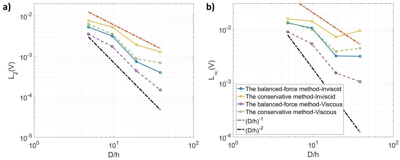
Figure 2: Results of the steady drops. a) $L_{2}$ and b) $L_{\infty}$ norms of the spurious current $V$($=|\mathbf{u}|$). a) and b) share the same legend. $(D/h)$ represents the spatial resolution where $D$ is the diameter of the Phase 1 drop and $h$ denotes the grid size.

5.1.3 Rising bubble: a convergence test

We perform a convergence test to quantify the convergence behavior of the numerical solution of the present mulitphase flow model to the sharp-interface solution. There are two convergence behaviors to consider when we numerically apply a Phase-Field based multiphase flow model. The first one is the convergence of the numerical solution to the exact solution of the multiphase flow model where the interface has a fixed thickness, as the cell size decreases. The second one is the convergence of the exact solution of the multiphase flow model to the sharp-interface solution, as the interface thickness decreases. In numerical implementations, it is more common and practical to consider those two together by decreasing both the cell size and the interface thickness at the same time, and then to evaluate how fast the numerical solution of the multiphase flow model converges to the sharp-interface solution. Hereafter in this section, we call the numerical solution of the present multiphase flow model from the present scheme in Section 4 as the Phase-Field solution.

The domain considered is $[1\times 2]$ and it has no-slip boundaries at the top and bottom but free-slip at the lateral. A bubble (Phase 1), whose density is 1 and viscosity is 0.1, is surrounded by Phase 2, whose density is 1000 and viscosity is 10. The density and viscosity ratios are 1000 and 100, respectively. The interfacial tension between them is 1.96, and the gravity is $\mathbf{g}=\{0,-0.98\}$. The cell size $h$ is ranging from $\frac{1}{16}$ to $\frac{1}{256}$, and the time step is $\Delta t=\mathrm{CFL}h$, where $\mathrm{CFL}=0.128$. We set $\eta=\eta_{0}\frac{h}{h_{0}}$, where $\eta_{0}$=$h_{0}=\frac{1}{32}$, and $M_{0}=10^{-7}\frac{\eta}{\eta_{0}}$, so that both of them decrease as the cell is refined. Initially, the bubble is at $(0.5,0.5)$ and its radius is 0.25. The computation is stopped at $t=1$. We use the circularity $\psi_{c}$ to quantify the shape of the bubble, while the dynamics of the bubble is quantified by the center of mass $y_{c}$ and the rising velocity $v_{c}$. These three benchmark quantities are defined as

$$\psi_{c}=\frac{P_{a}}{P_{b}}=\frac{2\sqrt{\int_{\phi_{1}>0}\pi d\Omega}}{P_{b}},$$ (66)

$$y_{c}=\frac{\int_{\Omega}y\frac{1+\phi_{1}}{2}d\Omega}{\int_{\Omega}\frac{1+\phi_{1}}{2}d\Omega},$$

$$v_{c}=\frac{\int_{\Omega}v\frac{1+\phi_{1}}{2}d\Omega}{\int_{\Omega}\frac{1+\phi_{1}}{2}d\Omega},$$

where $P_{a}$ is the perimeter of a circle whose area is identical to the bubble, and $P_{b}$ is the perimeter of the bubble. If the bubble is circular, $\psi_{c}$ is 1. Otherwise, it is less than 1. The same case was performed in (Hysingetal2009, ) using the sharp-interface models, where the Level-Set and the Arbitrary-Lagrange-Euler (ALE) methods were implemented and excellent agreements were reached in the time zone considered. The same benchmark quantities from the sharp-interface models are available in (Hysingetal2009, ) and they are considered as the references.

Fig.3 and Fig.4 show results using the balanced-force method and the conservative method, respectively. It is clear that the Phase-Field solution converges to the sharp-interface solution (labeled as “Reference” in the figures) as the cell size $h$, as well as the interface thickness $\eta$, reduces. To quantify the convergence rate, we compute the $L_{2}$ errors, i.e, the root mean square of the difference between the Phase-Field and the sharp-interface solutions, of the three benchmark quantities. The results are listed in Table 5, where “B-method” refers to the balanced-force method and “C-method” represents the conservative method. There is no significant difference between the results of the two methods, although the conservative method performs slightly better, giving smaller errors and faster convergence rates. Overall, both the circularity $\psi_{c}$ and the center of mass converge to their sharp-interface solutions with a rate close to second order, while the convergence rate of the rising velocity is slightly slower about 1.5th order.

In summary, the numerical solution of the present multiphase flow model from the present scheme in Section 4 converges to the sharp-interface solution, even in a case including large density and viscosity ratios. The convergence rate is between 1.5th- and 2nd-order.

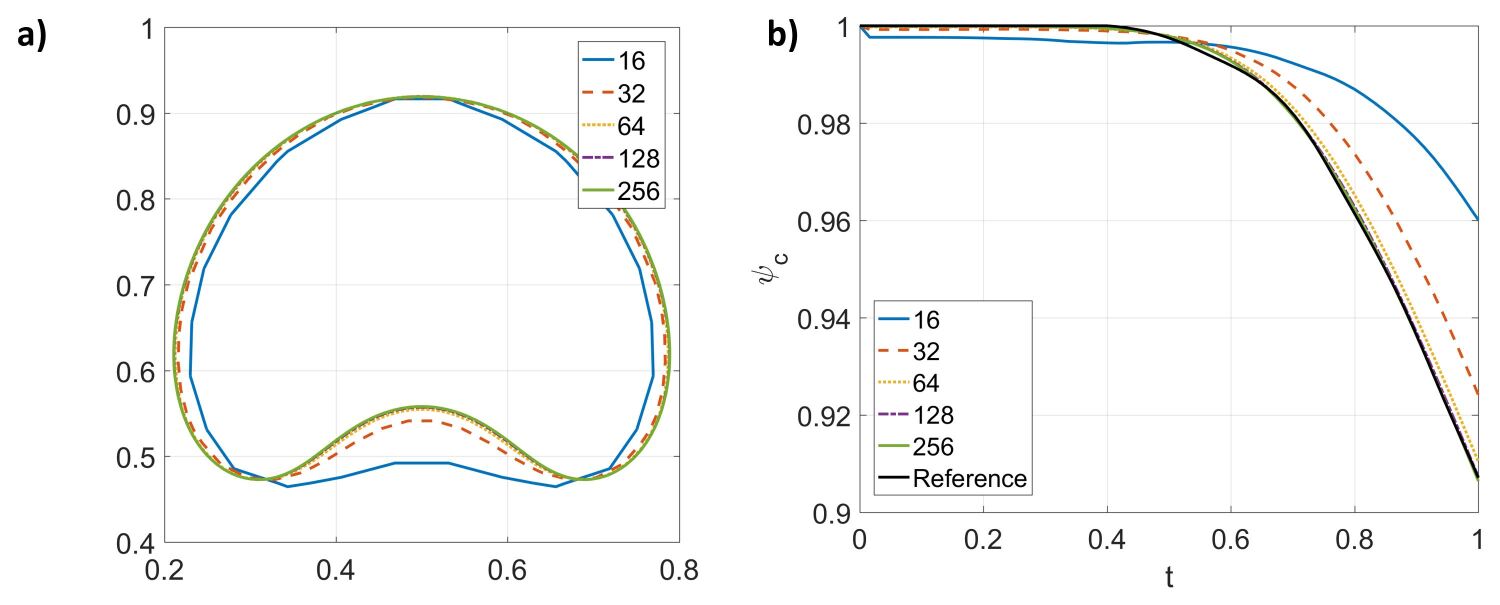
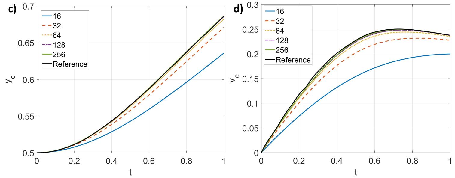
Figure 3: Results of the convergence test using the balanced-force method. a) Bubble shape at $t=1$. b) Circularity $\psi_{c}$ vs. $t$. c) Center of mass $y_{c}$ vs. $t$. d) Rising velocity $v_{c}$ vs. $t$. The legend shows the number of grid cells per unit length, and “Reference” is the sharp-interface solution from (Hysingetal2009, ).

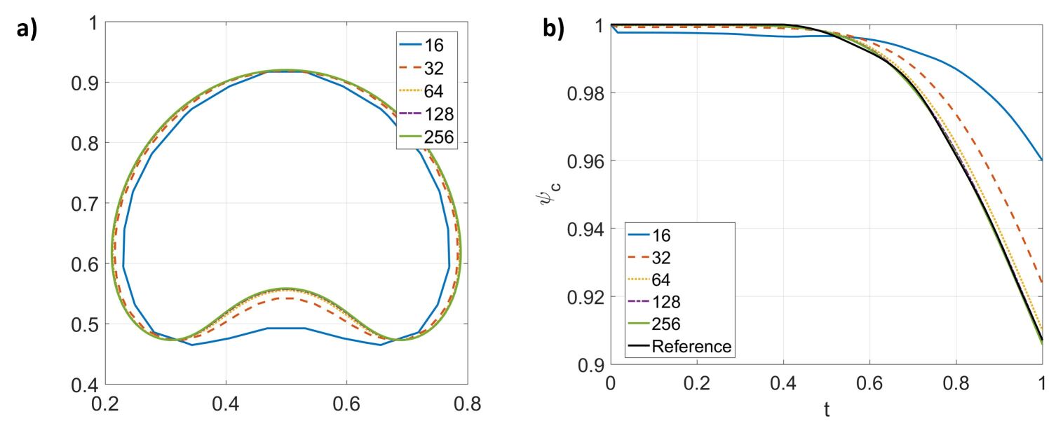
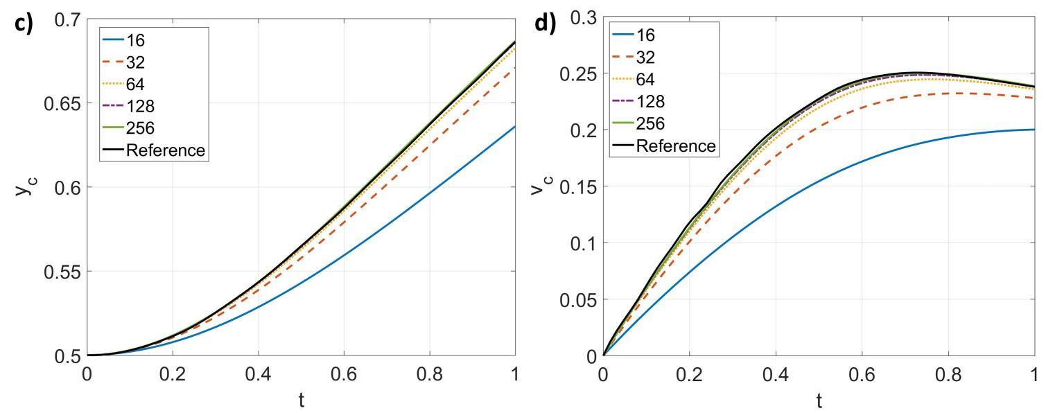
Figure 4: Results of the convergence test using the conservative method. a) Bubble shape at $t=1$. b) Circularity $\psi_{c}$ vs. $t$. c) Center of mass $y_{c}$ vs. $t$. d) Rising velocity $v_{c}$ vs. $t$. The legend shows the number of grid cells per unit length, and “Reference” is the sharp-interface solution from (Hysingetal2009, ).

Table 5: Results of the convergence test. B-method: the balanced-force method; C-method: the conservative method.

5.1.4 Large-density-ratio advection

We perform the large-density-ratio advection problem to demonstrate that the consistency of mass conservation and the consistency of mass and momentum transport are satisfied on the discrete level by the present scheme , and to illustrate the significance of satisfying these two consistency conditions. The domain considered is $[1\times 1]$ with doubly periodic boundaries. The material properties, unless otherwise specified, are $\rho_{1}=10^{9}$, $\rho_{2}=10^{6}$, and $\rho_{1}=1$ and there is neither viscosity nor interfacial tension. The cell size $h$ is $\frac{1}{128}$, and the time step is $\Delta t=\mathrm{CFL}h$, where $\mathrm{CFL}=0.1$. All the computations are stopped at $t=1$. We set $\eta$ to be $3h$ and $M_{0}$ to be $10^{-7}$. Initially, a circular drop (Phase 1) with a radius $0.1$ is at $(0.5,0.5)$, surrounded by Phase 2, whose outer interface is an ellipse with its semi-major axis 0.3 along the $y$ axis and with its semi-minor axis 0.25 along the $x$ axis. Both $u$ and $v$ are unity everywhere. Based on Theorem 4.4 in Section 4.3.1, the interfaces should be translated by the homogeneous velocity and therefore return to their original location at $t=1$ without any deformation. Moreover, the initial homogeneous velocity should not be changed, thanks to satisfying the consistency of mass conservation and the consistency of mass and momentum transport on the discrete level.

Fig.5 a) and c) show the result from the present scheme. It can be observed that the interfaces, as expected, return to their initial location without any deformation, and all the streamlines are straightly pointing towards $45^{0}$, as what they were at $t=0$. Fig.5 b) and d) show the result from an inconsistent mass flux, i.e., using $\langle\mathbf{m}\rangle=\overline{\rho}\mathbf{u}$. Due to violating the consistency conditions, the interfaces experience significant unphysical deformations and the streamlines are fluctuating. It should be noted that the densities of the phases are $1000$, $10$, and $1$, respectively, in the case using the inconsistent mass flux, in order to have a stable solution up to $t=1$.

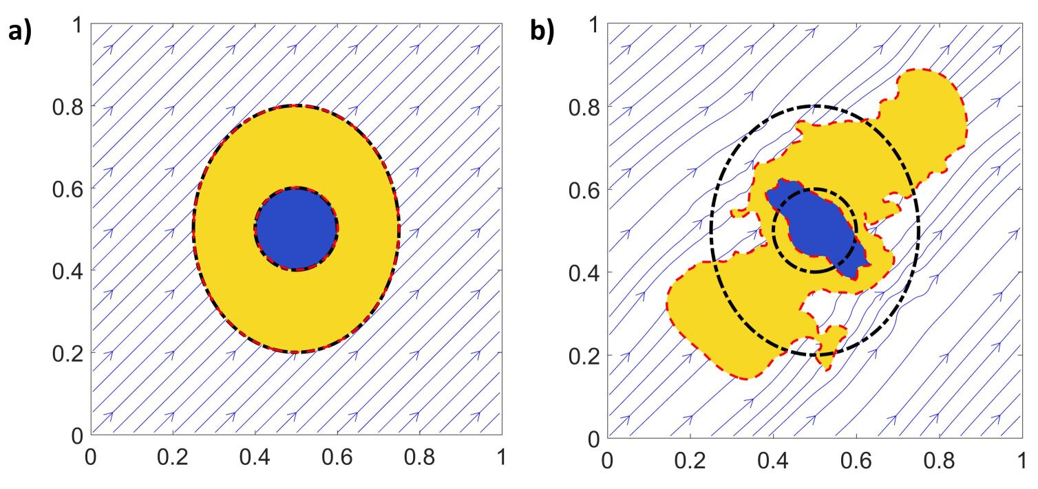
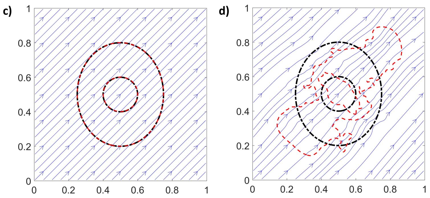
Figure 5: Results of Large-density-ratio advection. a) and c) Results from the present scheme with densities $\rho_{1}=10^{9}$, $\rho_{2}=10^{6}$, and $\rho_{1}=1$. b) and d) Results of using the inconsistent mass flux with densities $\rho_{1}=10^{3}$, $\rho_{2}=10$, and $\rho_{1}=1$. Blue arrow lines: Streamlines at $t=1$, Black dash-dotted lines: Interfaces at $t=0$, Red dashed lines: Interfaces at $t=1$, Blue: Phase 1, Yellow: Phase 2, Background: Phase 3.

In summary, the present scheme satisfies the consistency of mass conservation and the consistency of mass and momentum transport on the discrete level, and Theorem 4.4 in Section 4.3.1 is validated.

5.1.5 Horizontal shear layer

We perform the horizontal shear layer problem to validate the consistency of reduction, summation of the order parameters, and mass and momentum conservation of the present scheme, and further to discuss the energy law on the discrete level. Different layers of fluids are moving horizontally at different speeds. A vertical velocity perturbation is applied and the fluids begin to interact with each other. The domain considered is $[1\times 1]$ and all its boundaries are periodic. We use $[128\times 128]$ cells to discretize the domain in default, and the time step is $\Delta t=\mathrm{CFL}h$, where $h$ is the cell size and $\mathrm{CFL}$ is $0.1$. The material properties, unless otherwise specified, are $\rho_{1}=50$, $\rho_{2}=10$, $\rho_{3}=1$, $\rho_{4}=0.5$, $\mu_{1}=0.01$, $\mu_{2}=0.1$, $\mu_{3}=0.05$, $\mu_{4}=0.08$, $\sigma_{1,2}=0.05$, $\sigma_{1,3}=0.01$, $\sigma_{1,4}=0.08$, $\sigma_{2,3}=0.1$, $\sigma_{2,4}=0.02$, $\sigma_{3,4}=0.2$. $\eta$ and $M_{0}$ are $\frac{1}{128}$ and $10^{-7}$, respectively. Initially, Phase 1 is stationary in $y_{0}<y<y_{2}$, Phase 2 is in $y_{1}<y<y_{0}$, moving from the left to right at a unity speed, and Phase 3 moves in the opposite direction, filling the rest of the domain. Phase 4 is absent, i.e., $\phi_{4}|_{t=0}=-1$. We set $y_{0}=0.5$, $y_{1}=0.25$, and $y_{2}=0.75$. This configuration is perturbed by a vertical velocity $v|_{t=0}=\delta\sin(k_{0}x)$, where $\delta=0.05$ and $k_{0}=2\pi$.

We first validate the consistency of reduction on the discrete level. From Theorem 4.1 in Section 4.1.1, $\phi_{4}$, which is absent at the beginning of the computation, should not appear during the computation, i.e., $\phi_{4}\equiv-1$. In addition, since Phase 4 is absent, the problem considered is actually a three-phase problem. The result from setting $N=4$ and $\phi_{4}|_{t=0}=-1$ should be the same as that from setting $N=3$. Fig.6 a) shows the time history of the maximum value of $|\phi_{4}+1|$. It is clear that $\phi_{4}$ equals to $-1$ up to the round off error. Fig.6 b) shows the time histories of the kinetic energy $E_{K}$ ($=\sum_{i,j}[e_{K}]_{i,j}\Delta\Omega$), the free energy $E_{F}$ ($=\sum_{i,j}[e_{F}]_{i,j}\Delta\Omega$), and the total energy $E_{T}$ ($=E_{K}+\frac{1}{2}E_{F}$) from the 4-phase and 3-phase solutions, and they are indistinguishable from each other. Fig.6 c) and d) show the snapshots of the three phases at $t=2$ from the 4-phase and 3-phase solutions, respectively, and they are identical. The results validate that the consistency of reduction is satisfied by the present scheme on the discrete level. Instead of applying the present scheme, where all the order parameters are numerically solved from their Phase-Field equation, we repeat the 4-phase setup and follow the practice in (Dong2018, ), where only $\phi_{1}$, $\phi_{2}$, and $\phi_{3}$ are numerically solved from their Phase-Field equation and $\phi_{4}$ is algebraically obtained from their summation, i.e., $\phi_{4}=-2-(\phi_{1}+\phi_{2}+\phi_{3})$. The result is shown in Fig.7. It can be observed that Phase 4, which is absent at the beginning, is being generated numerically, and, therefore, the consistency of reduction is violated on the discrete level, although the summation of the order parameters, i.e., Eq.(4), is exactly enforced. As discussed in Section 3.2, $\{\widetilde{\phi_{p}}\}_{p=1}^{3}$ in the convection term of the Phase-Field equation do not follow $\sum_{p=1}^{3}\widetilde{\phi_{p}}=-1$ because they are computed independently from the WENO scheme. This error contributes to $\sum_{p=1}^{3}\phi_{p}\neq-1$, and consequently, $\phi_{4}=-2-(\phi_{1}+\phi_{2}+\phi_{3})$ can be larger than $-1$. In other words, $\phi_{4}$ is generated numerically. This numerical test highlights that even though the Phase-Field equation satisfies the consistency of reduction, its numerical scheme still needs to be carefully designed in order to preserve this property and, consequently, to avoid generating fictitious phases numerically. Since we have validated that the present scheme satisfies the consistency of reduction, in the rest of this section, we only use the 3-phase solution.

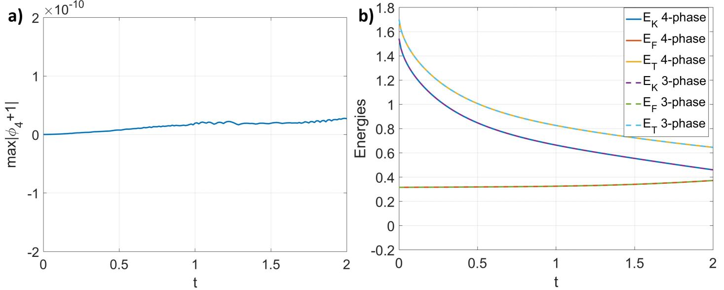
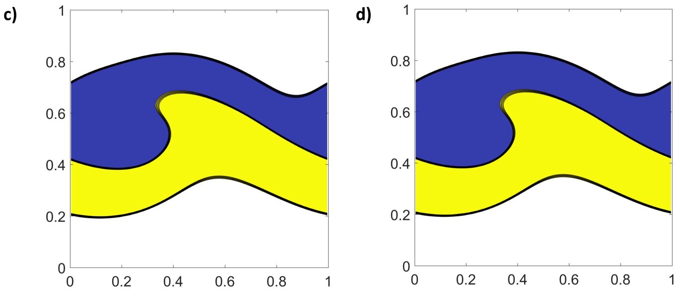
Figure 6: Validation of the consistency of reduction. a) Time history of $\mathrm{max}|\phi_{4}+1|$. b) Time histories of the kinetic, free and total energies from the 4-phase and 3-phase solutions. c) Snapshot of the phases at $t=2$ from the 4-phase solution. d) Snapshot of the phases at $t=2$ from the 3-phase solution. Blue: Phase 1, Yellow: Phase 2, White: Phase 3.

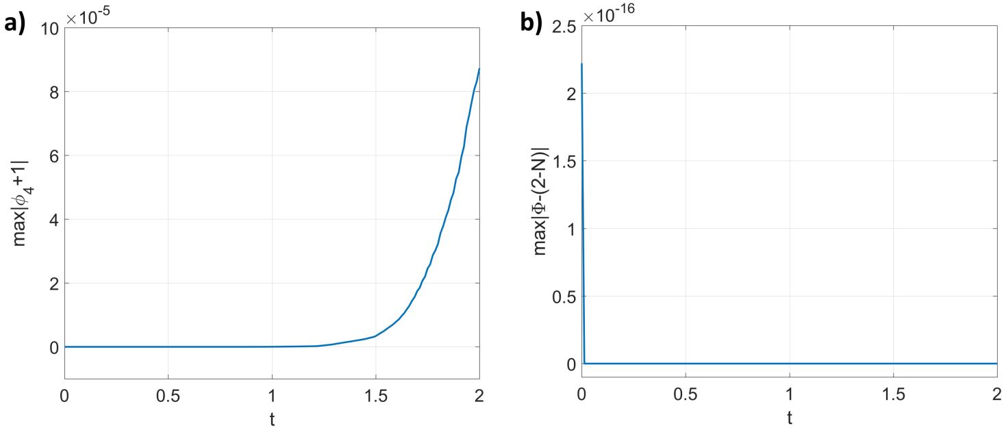
Figure 7: Generation of fictitious phases from a reduction inconsistent scheme: solving $\phi_{1}$, $\phi_{2}$, and $\phi_{3}$ numerically from their Phase-Field equation and obtaining $\phi_{4}$ algebraically from $\phi_{4}=-2-(\phi_{1}+\phi_{2}+\phi_{3})$. a) Time history of $\mathrm{max}|\phi_{4}+1|$. b) Time history of $\mathrm{max}|\Phi-(2-N)|$ ($\Phi=\sum_{p=1}^{N}\phi_{p}$).

We next consider the mass conservation and the summation of the order parameters on the discrete level. From Theorem 4.3 in Section 4.1.1, the order parameters and therefore the mass of fluid mixture are conserved, i.e., $\mathrm{Mass}=\sum_{i,j}[\rho]_{i,j}\Delta\Omega$ and $\mathrm{M}_{p}=\sum_{i,j}[\phi_{p}]_{i,j}\Delta\Omega$ do not change with time. In addition, from Theorem 4.2, $\Phi=\sum_{p=1}^{N}\phi_{p}=(2-N)$ is true at every cell center, which avoids generating local voids or overfilling. Fig.8 a) and b) show that the changes of $\mathrm{Mass}$ and $\mathrm{M}_{p}$, respectively, are the machine zero. These results confirm that the mass conservation is satisfied by the present scheme on the discrete level. Fig.8 c) and d) show the results including the gradient-based phase selection procedure (Present) and using the WENO scheme only (WENO), respectively. Because of the non-linearity of the WENO scheme, the summation and the interpolation are not commutable. As a result, $\sum_{p=1}^{N}\tilde{\nabla}\cdot(\mathbf{u}\widetilde{\phi_{p}})$ is not zero, which leads to $\Phi\neq(2-N)$. Besides, the difference between $\Phi$ and $(2-N)$ increases with time, as shown in Fig.8 c), although the difference between $\Phi^{n+1}$ and $\Phi^{n}$ at the beginning is tiny. The error is accumulating and finally becomes noticeable in long-time simulations. Physically speaking, this error corresponds to generating local voids or overfilling. On the contrary, the present scheme, which implements the gradient-based phase selection procedure, guarantees $\Phi=(2-N)$ all the time. Fig.8 d) shows the spatial distribution of $\Phi-(2-N)$ at $t=2$. The present scheme guarantees $\Phi=(2-N)$ at every cell center, while only using the WENO scheme generates local voids or overfilling at about one third of the total discrete cells.

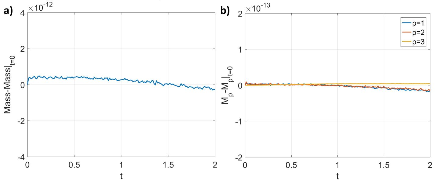
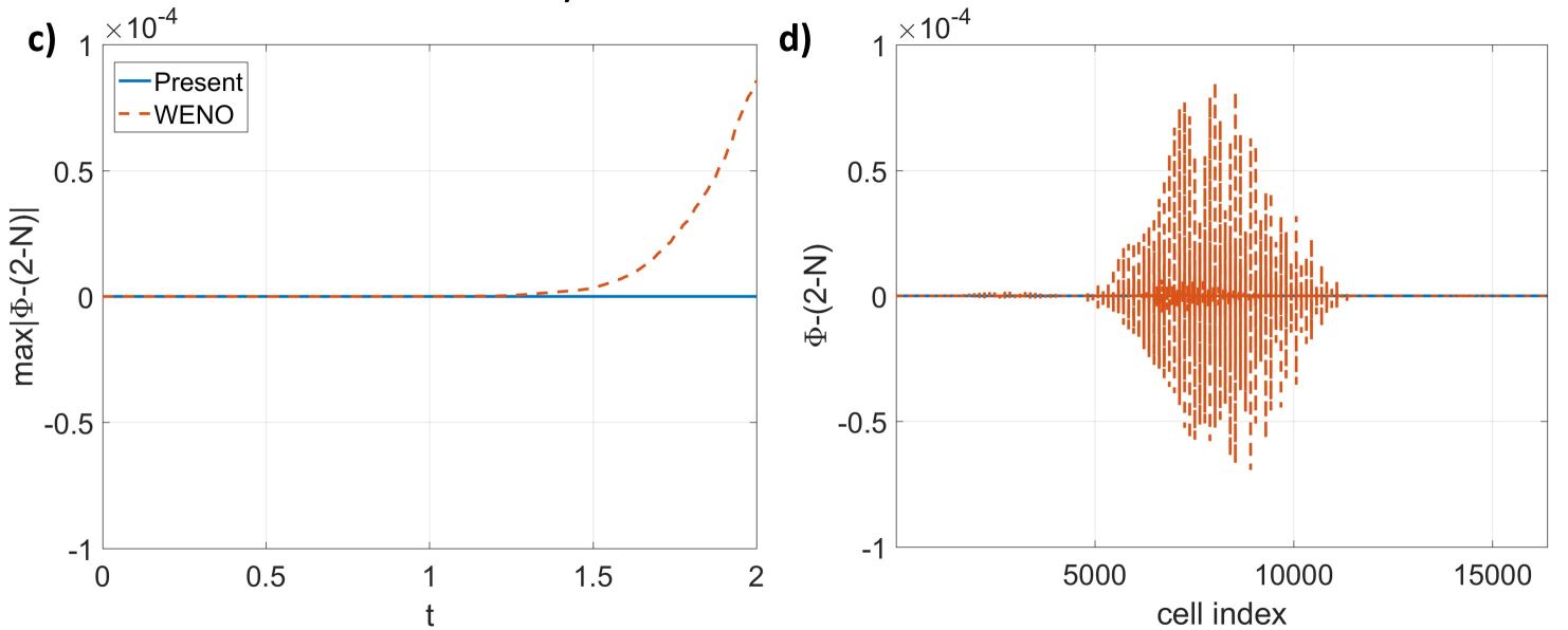
Figure 8: Validation of the mass conservation and summation of the order parameters. a) Time history of the change of $\mathrm{Mass}$($=\sum_{i,j}[\rho]_{i,j}\Delta\Omega$). b) Time histories of the change of $\mathrm{M}_{p}$($=\sum_{i,j}[\phi_{p}]_{i,j}\Delta\Omega$). c) Time histories of $\mathrm{max}|\Phi-(2-N)|$ ($\Phi=\sum_{p=1}^{N}\phi_{p}$) from the present scheme including the gradient-based phase selection procedure (Present) and the scheme using WENO only (WENO). d) Spatial distributions of $\Phi-(2-N)$ at $t=2$ from the present scheme and the scheme using WENO only. c) and d) share the same legend.

We now consider the momentum conservation on the discrete level. From Theorem 4.5 and Corollary 4.5.1 in Section 4.3.1, the momentum is conserved, i.e., $\mathrm{\mathbf{Momentum}}=\sum_{i,j}[\rho\mathbf{u}]_{i,j}\Delta\Omega$ does not change with time, if the conservative method is used to compute the surface force in Eq.(23). However, this is not necessarily true when the balanced-force method is implemented. Results in Fig.9 a) and b) confirm our analysis. The momentum from the balanced-force method increases with time in this case, although it is not significant. Quantitatively, the change of $\mathrm{Momentum}_{x}$ is less than $0.04\%$ of its initial value. On the other hand, the momentum from the conservative method does not change with time. Since the difference between the balanced-force method and the conservative method is in the order of the truncation error, the non-conservation of the momentum from the balanced-force method should be reduced under grid refinement, and this is also shown in Fig.9 a) and b). Fig.9 c) and d) show the snapshots of the three phases from the balanced-force method and the conservative method, respectively. The difference is very small. We summarize that, on the discrete level, the momentum is conserved by the present scheme if the conservative method is used, while it is essentially conserved if the balanced-force method is used.

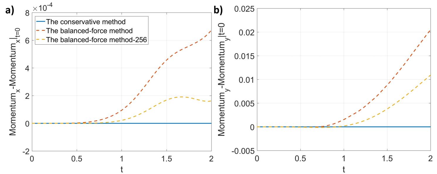
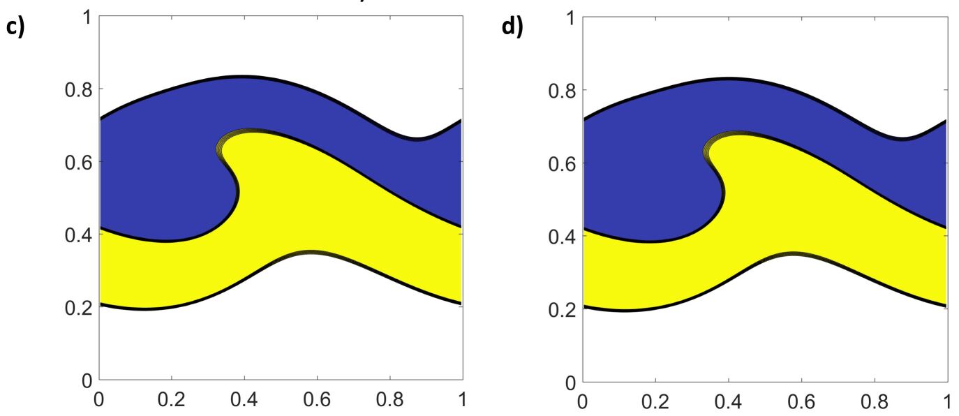
Figure 9: Validation of the momentum conservation. a) Time history of the change of $\mathrm{Momentum}_{x}$(=$\sum_{i,j}[\rho u]_{i,j}\Delta\Omega$). b) Time histories of the change of $\mathrm{Momentum}_{y}$(=$\sum_{i,j}[\rho v]_{i,j}\Delta\Omega$). a) and b) share the same legend, and “256” in the legend represents the results obtained from a finer cell size $h=\frac{1}{256}$. c) Snapshot of the phases at $t=2$ from the balanced-force method. d) Snapshot of the phases at $t=2$ from the conservative method. Blue: Phase 1, Yellow: Phase 2, White: Phase 3.

We finally consider the energy law of the present multiphase flow model, i.e., Eq.(22), on the discrete level. We will show through the following numerical experiments that the present scheme reproduces the behaviors of the energy law.

In the first case, where there is neither viscosity nor interfacial tension, the free energy is zero so the total energy is the same as the kinetic energy. From the energy law in Eq.(22), the total energy, the same as the kinetic energy in this case, does not change with time. However, in practice, the total energy is decreased due to numerical dissipation. Fig.10 shows the time histories of the kinetic, free, and total energies. The free energy is identically zero, while the kinetic energy and the total energy are decaying. When we refine the cell, the change of the kinetic energy is reduced, implying that the numerical dissipation is the source of changing the kinetic energy. The numerical dissipation comes from the backward difference in time, the WENO scheme for the interpolation, and the linearly interpolated pressure gradient in Eq.(63).

Figure 10: Time histories of the kinetic ($E_{K}$), free ($E_{F}$), and total ($E_{T}$) energies in the case without viscosity and interfacial tensions. “256” in the legend: Results obtained from a finer cell size $h=\frac{1}{256}$.

The second case has no viscosity but interfacial tensions. From Eq.(22), there is energy transfer between the kinetic energy and the free energy in this case, while the total energy should decrease. Fig.11 shows the results from the balanced-force method and the conservative method. Both methods produce results that respect the energy law, i.e., the total energy decreases with time, as shown in Fig.11 a) and b). We can also observe the energy transfer from the kinetic energy to the free energy due to the deformation of the initial flat interfaces. In Fig.11 c), although the total energies from the two methods are very close to each other, the kinetic energy from the conservative method decreases more than the one from the balanced-force method at a later time in this case. As a result, the free energy from the conservative method increases faster than the one from the balanced-force method. The difference between the two methods is much less after we refine the cell size, as shown in Fig.11 d).

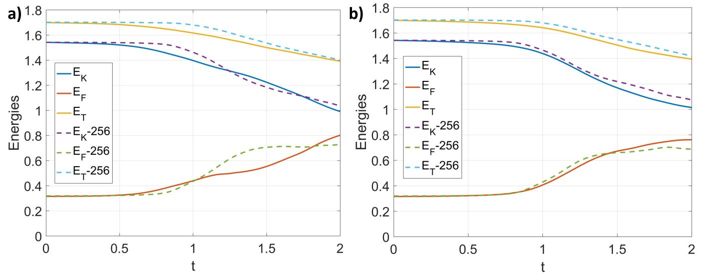
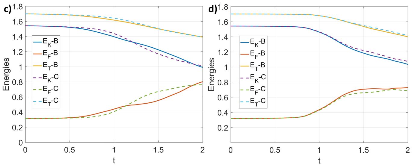
Figure 11: Time histories of the kinetic ($E_{K}$), free ($E_{F}$), and total ($E_{T}$) energies in the case without viscosity but with interfacial tensions. a) from the balanced-force method. b) from the conservative method. c) from the cell size $h=\frac{1}{128}$. d) from the cell size $h=\frac{1}{256}$. B: The balanced-force method, C: The conservative method, “256”: Results obtained from a finer cell size $h=\frac{1}{256}$.

The last case considered includes both viscosity and interfacial tensions, corresponding to the complete form of Eq.(22). The results are shown in Fig.12, and both the balanced-force method and the conservative method produce results that follow Eq.(22), as shown in Fig.12 a) and b). There is little difference between the default and the fine grid solutions, implying that the decay of the total energy results from the physical interaction in the multiphase flow model, instead of numerical dissipation. In addition, the difference between the two methods is hardly observable in both the default and the find grid solutions, as shown in Fig.12 c) and d).

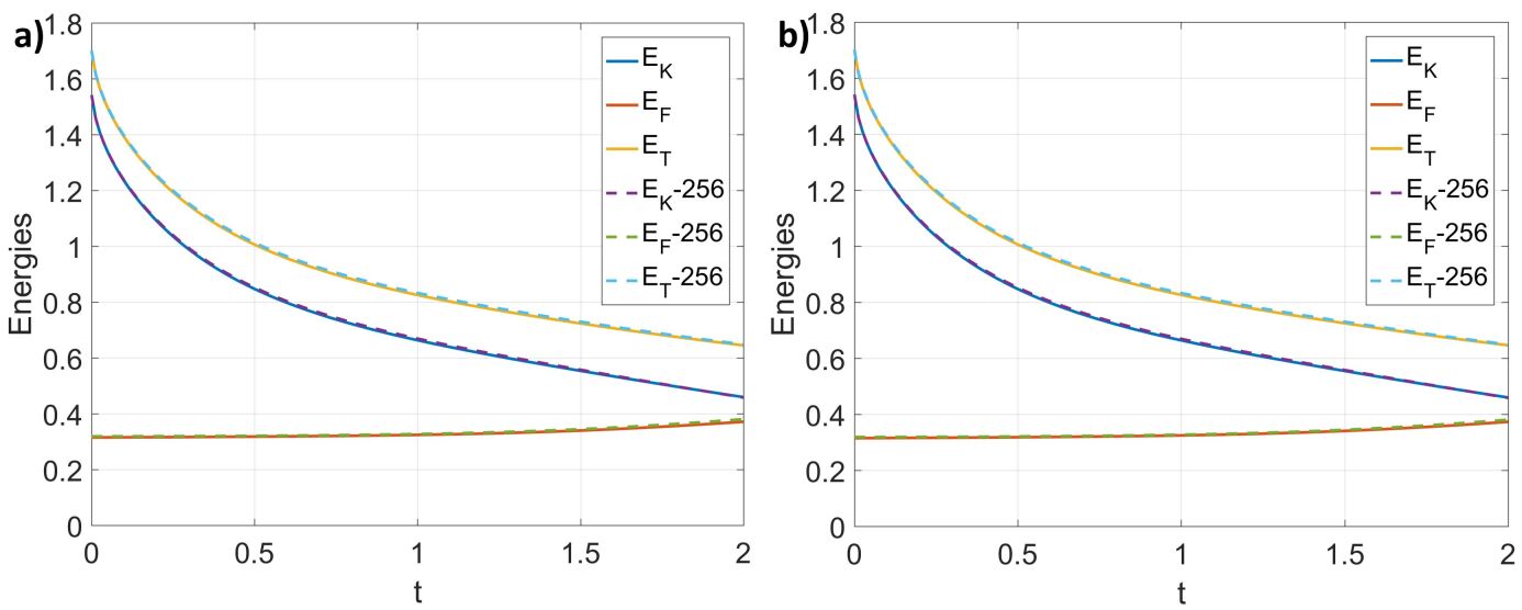
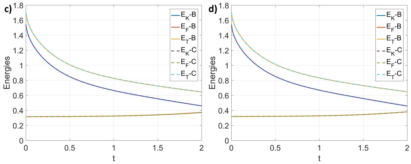
Figure 12: Time histories of the kinetic ($E_{K}$), free ($E_{F}$), and total ($E_{T}$) energies in the case with viscosity and interfacial tensions. a) from the balanced-force method. b) from the conservative method. c) from the cell size $h=\frac{1}{128}$. d) from the cell size $h=\frac{1}{256}$. B: The balanced-force method, C: The conservative method, “256”: Results obtained from a finer cell size $h=\frac{1}{256}$.

In summary, the following properties of the present scheme analyzed in Section 4 are validated. The present scheme satisfies the consistency of reduction, mass conservation, and summation of the order parameters. The momentum, on the discrete level, is conserved when the conservative method is used to compute the surface force, while it is essentially conserved when the balanced-force method is used. Moreover, the behaviors of the energy law of the present multiphase flow model is reproduced.

5.2 Application

In this section, we apply the present mutliphase flow model and scheme to various realistic multiphase flow problems to further verify their capability. The water, oil, and air have the material properties in Table 6, and the contact angles, if needed, are all $\frac{\pi}{2}$, unless otherwise specified. Results are reported in their dimensionless forms under $\eta=0.01$ and $M_{0}=10^{-7}$.

Table 6: Material properties of the water, air, and oil.

5.2.1 Three-phase Rayleigh-Taylor instability

We consider a three-phase Rayleigh-Taylor instability problem, where the heaviest phase (Phase 1) stays on the top of Phase 2, whose density is in the middle. At the bottom, there is the lightest phase (Phase 3). The Atwood number between Phases $p$ and $q$ is defined as $At_{p,q}=\frac{\rho_{p}-\rho_{q}}{\rho_{p}+\rho_{q}}$. The domain of interest is $1\times 6$. Its left and right boundaries are periodic while the top and bottom boundaries are free-slip. We use $128\times 768$ cells to discretize the domain and the time step is $\Delta t=10^{-3}$. The densities of the fluids are $\rho_{1}=4.5,\rho_{2}=3,\rho_{3}=1$, and their dynamic viscosities are all $10^{-3}$. As a result, we have $At_{1,2}=0.2$ and $At_{2,3}=0.5$. The pairwise interfacial tensions are $\sigma_{p,q}=10^{-12},p\neq q$. The gravity is pointing downward with a magnitude of unity, i.e., $\mathbf{g}=\{0,-1\}$. Here, the chosen material properties follow the setups in (Tryggvason1988, ; GuermondQuartapelle2000, ; Dingetal2007, ; Huangetal2019, ; Huangetal2020, ), so that we can compare interface locations from the present model to existing numerical data. Initially, the flow is stationary, and the interface between Phases 1 and 2 is at $y=4$ and that between 2 and 3 is at $y=2$. A horizontal sinusoidal perturbation is applied to both of the interfaces, whose amplitude is 0.1 and wavelength is $2\pi$.

Since the interfaces are initially far away separated, there is no interaction between them, and the three-phase Rayleigh-Taylor instability problem is actually a combination of two independent two-phase Rayleigh-Taylor instability problems at the beginning of the simulation. As a result, we can compare the locations of the interface between Phases 2 and 3 at the center and at the lateral edge of the domain to the two-phase results in (Tryggvason1988, ; GuermondQuartapelle2000, ; Dingetal2007, ; Huangetal2019, ; Huangetal2020, ), where the Atwood number $At$ is 0.5. The comparisons are shown in Fig.13, and the present results under a three-phase setup are hardly distinguished from the published ones under a two-phase setup.

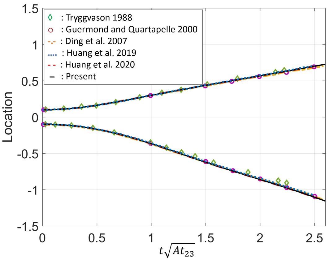
Figure 13: Locations of the interface between Phases 2 and 3 at the center (bottom curves) and at the lateral (top curves) of the domain in the three-phase Rayleigh-Taylor instability problem.

The evolution of the three phases is presented in Fig.14 up to $t=10$. Before $t=5$, the three-phase dynamics is not observed, and the interfaces between Phases 1 and 2 and between Phases 2 and 3 evolve independently, without noticing the existence of an additional phase. The configurations of the individual interfaces are almost identical to those reported in (Dingetal2007, ; Huangetal2019, ; Huangetal2020, ) where only two phases were considered. Phase 2 moves downward faster than Phase 1 because the Atwood number between Phases 2 and 3 is larger than that between Phases 1 and 2. We can observe multiple droplets and filaments being generated from Phase 2 before it reaches the bottom of the domain. After $t=5$, the three-phase dynamics begins. Phase 2 accumulates at the bottom of the domain, and then moves upward along the lateral edge of the domain. A channel of Phase 2 is built up in the middle of the domain and Phase 1 tries to move downward along this channel. As a result, the configuration of the interface between Phases 1 and 2 is shrunk compared to the two-phase one in (Huangetal2019, ). Phase 1 gradually fills up the middle channel, producing complex patterns resulting from its strong interactions with the other phases. Since Phase 1 is the heaviest, it takes the place of Phase 2 at the bottom and the lateral edge of the domain at the end of the simulation. As a result, Phase 2 is pushed to aggregate between the middle and lateral columns of Phase 1. The long-time dynamics of this problem is highly sophisticated because of the strong interactions between the three phases.

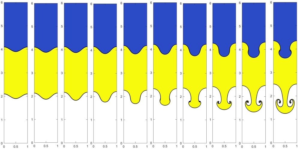
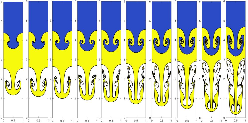
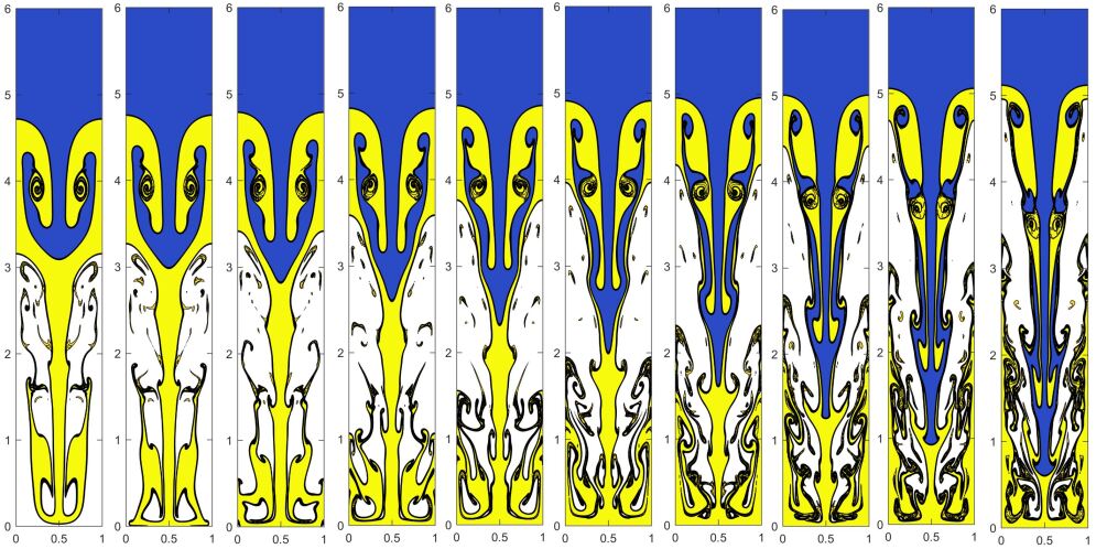
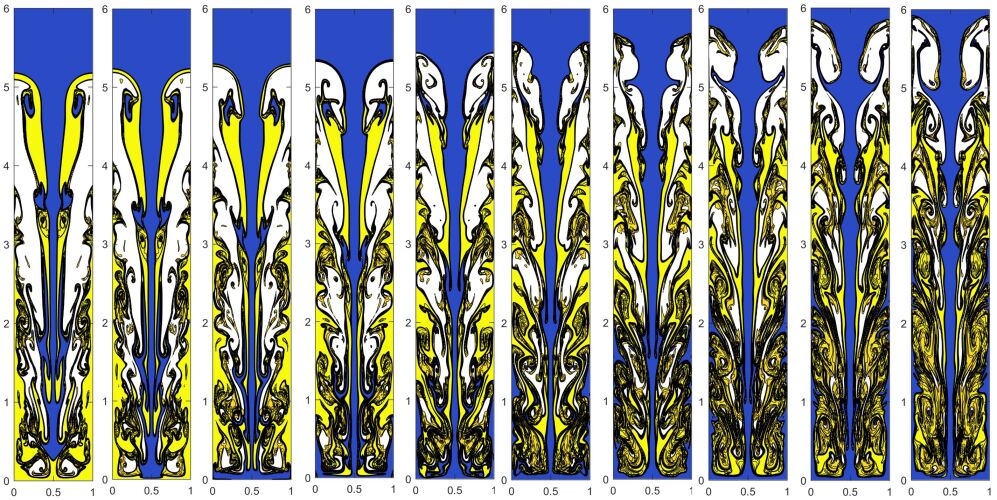
Figure 14: Evolution of the three phases in the three-phase Rayleigh-Taylor instability problem. From left to right, top to bottom, $t$ is 0.00, 0.50, 0.75, 1.00, …, 10.00. Blue: Phase1, Yellow: Phase2, and White: Phase3.

5.2.2 Floating liquid lens

We perform the floating liquid lens problem to investigate the equilibrium states of the multiphase flows. An oil drop (Phase 2) is floating on the interface between the water (Phase 1) at the bottom and the air (Phase 3) on the top. Because the forces are imbalanced at the triple points of the three phases, the drop will be stretched horizontally while compressed vertically and finally reaches its equilibrium state. If there is no gravity, we can derive an exact solution based on the force balance at the triple points, the normal stress balance at the interfaces, and the mass conservation. Details of the derivation are provided in Appendix. If the gravity is dominant, asymptotic analyses from Langmuir and de Gennes (Langmuir1933, ; deGennesetal2003, ) give the final thickness of the drop as

$$e_{d}=\sqrt{\frac{2(\sigma_{2,3}+\sigma_{1,2}-\sigma_{1,3})\rho_{1}}{\rho_{2}(\rho_{1}-\rho_{2})|\mathbf{g}|}}.$$ (67)

The material properties are listed in Table 6. Non-dimensionalization is performed based on a density scale $1.2041\mathrm{kg/m^{3}}$, a length scale $0.04\mathrm{m}$, and an acceleration scale $1\mathrm{m/s^{2}}$. After that, the domain considered is $[-1,1]\times[0,0.8]$ with periodic boundaries at the lateral and no-slip walls at the top and bottom. The domain is discretized by $[201\times 81]$ cells and the time step is $\Delta t=10^{-5}$. Initially, a circular oil drop (Phase 2) of a radius 0.2 is at $(0,0.4)$, floating on the horizontal interface between the water (Phase 1) and the air (Phase 3) at $y=0.4$. We consider three different magnitudes of the gravity, i.e., $|\mathbf{g}|=0,5,9.8$, and the direction of the gravity is pointing downward.

Fig.15 shows the final thickness of the oil drop (Phase 2) with respect to the magnitude of the gravity, along with the exact solution for the zero gravity and with the asymptotic solution Eq.(67). Our numerical results match both the exact and asymptotic solutions in the two limits very well.

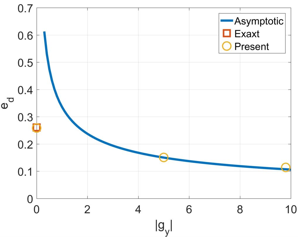
Figure 15: Final thickness of the drop vs. magnitude of the gravity in the floating liquid lens problem.

Fig.16 shows the initial and final shapes of the three phases. When there is no gravity, the drop becomes a combination of two circular segments, which agrees well with the exact solution. As the gravity increases, the drop is horizontally elongated and vertically compressed.

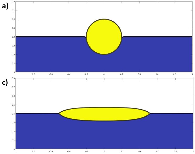
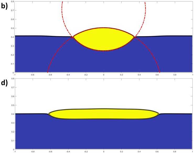
Figure 16: Initial and final shapes of the three phases in the floating liquid lens problem. a) Initial shapes. b) Final shapes with $|\mathbf{g}|=0$. c) Final shapes with $|\mathbf{g}|=5$. d) Final shapes with $|\mathbf{g}|=9.8$. Blue: Phase 1, Yellow: Phase 2, White: Phase 3. Red dash-dotted lines in b): Exact solution for $|\mathbf{g}|=0$.

5.2.3 Drops on a surface

In this case, we include the effect of the contact angles, and investigate the equilibrium shapes of the drops on a flat surface. Without considering the gravity, any semi-circular drop, whose radius is $R_{0}$, on a homogeneous solid wall will finally reach an equilibrium state that it becomes a circular segment with a radius $R$, height $H_{d}$, and spreading length $L_{d}$ as

$$R = R_{0}\sqrt{\frac{\pi/2}{\theta_{s}-\cos(\theta_{s})\sin(\theta_{s})}},$$ (68)

$$H_{d} = R\left(1-\cos(\theta_{s})\right),$$

$$L_{d} = 2R\sin(\theta_{s}),$$

where $\theta_{s}$, measured by radian, is the contact angle between the drop and the wall. The derivation of Eq.(68) is provided in Appendix. We consider three phases appearing in the domain, where the water (Phase 1) is in contact with the bottom wall, the oil (Phase 2) is in contact with the top wall, and the air (Phase 3) fills the rest of the domain. The material properties of the phases are the same as those in Table 6 except $\rho_{2}=870\mathrm{kg/m^{3}}$ and $\mu_{3}=1.78\times 10^{-4}\mathrm{Pa\cdot s}$ in this case. Non-dimensionalization is performed based on a density scale $1.2041\mathrm{kg/m^{3}}$, a length scale $0.04\mathrm{m}$, and an acceleration scale $1\mathrm{m/s^{2}}$. After that, the domain considered is $[-1,1]\times[0,0.5]$ with periodic boundaries at the lateral and no-slip walls at the top and bottom. The domain is discretized by $[200\times 50]$ cells and the time step is $\Delta t=10^{-4}$. Three sets of the contact angles between Phases 1 and 3 at the bottom wall and between Phases 2 and 3 at the top wall are $(45^{0},135^{0})$, $(120^{0},60^{0})$, and $(75^{0},105^{0})$. Initially, the centers of Phases 1 and 2 are at $(-0.5,0)$ and $(0.5,0.5)$, respectively, and both of them are semi-circular with a radius $R_{0}=0.2$.

Fig.17 shows the heights and the spreading lengths obtained from the numerical solutions under different contact angles, along with the exact solution from Eq.(68). Our numerical results agree well with the exact solution.

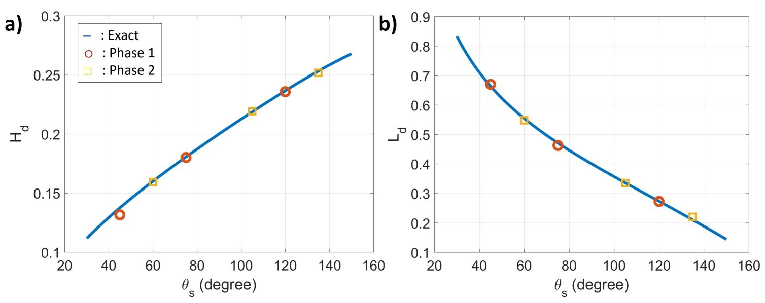
Figure 17: Heights and spreading lengths of the drops on a surface. a) Height ($H_{d}$) vs. contact angle ($\theta_{s}$). b) Spreading length ($L_{d}$) vs. contact angle ($\theta_{s}$). a) and b) share the same legend.

Fig.18 shows the initial and final shapes of the drops, along with the circular segments determined from Eq.(68). The interfaces between Phases 1 and 3 and between Phases 2 and 3 overlap onto those circular segments, which are the exact equilibrium shapes of the drops.

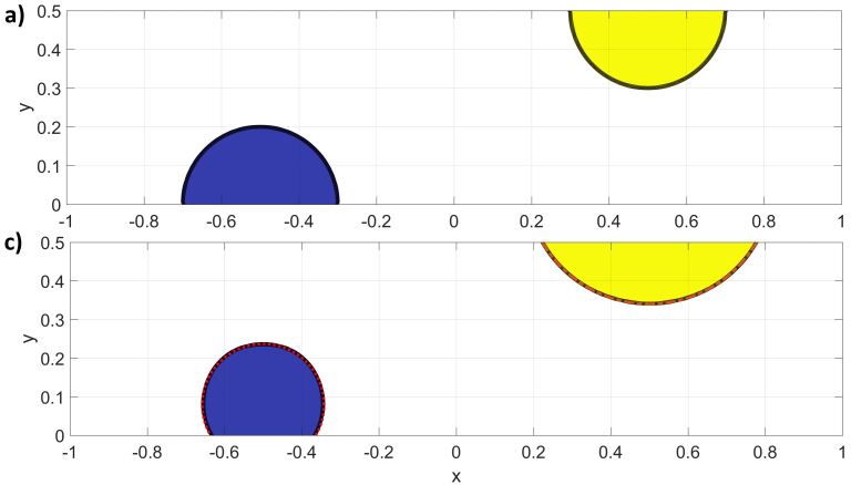
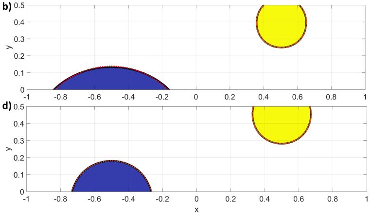
Figure 18: Initial and final shapes of the drops on a surface. a) Initial shapes. b) Final shapes with contact angles $(45^{0},135^{0})$. c) Final shapes with contact angles $(120^{0},60^{0})$. d) Final shapes with contact angles $(75^{0},105^{0})$. Blue: Phase 1, Yellow: Phase 2, White: Phase 3. Red dotted line: Exact equilibrium shape of Phase 1, Orange dash-dotted line: Exact equilibrium shape of Phase 2.

5.2.4 Three-phase dam break

We consider a three-phase dam break problem, where the water (Phase 1), oil (Phase 2), and air (Phase 3) interact with each other. Their material properties are listed in Table 6. Non-dimensionalization is performed based on a density scale $1.2041\mathrm{kg/m^{3}}$, a length scale $0.05715\mathrm{m}$, and an acceleration scale $9.8\mathrm{m/s^{2}}$. After that, the domain considered is $[8\times 2]$ and all the domain boundaries are no-slip. The domain is discretized by $[512\times 128]$ cells and the time step is $\Delta t=5\times 10^{-4}$. Initially, the water column has a unit height and is at the left of the domain, while the oil column is at the right, as high as the water column, and the fluids are stationary.

Because of the gravity, both the water and oil columns will collapse. Since the water and oil are initially separated far enough, the motion of the water should not be influenced by the oil at the beginning of the dynamics. Thus, we can compare the locations of the front $Z$ and the height $H$ of the water column to the experimental measurements by Martin and Moyce (MartinMoyce1952, ) and to the two-phase (water-air) results by Huang et al. (Huangetal2020, ). We calibrated the data by setting $Z=1.44$ at $t=0.8$ and $H=1$ at $t=0$, like those in (MartinMoyce1952, ). The comparisons are shown in Fig.19, and the present results not only agree well with the experimental measurements but also are almost the same as the two-phase solution.

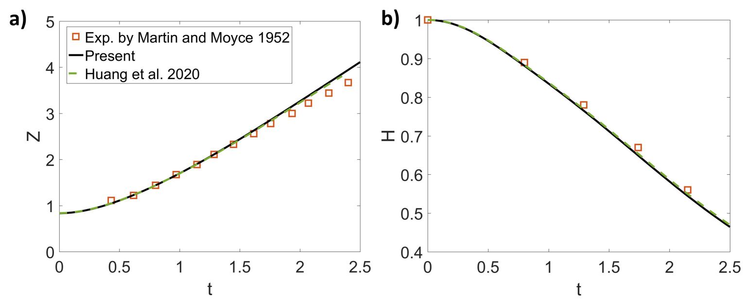
Figure 19: Front and height of the water column in the three-phase dam break problem. a) Front ($Z$) vs. $t$. b) Height ($H$) vs. $t$. a) and b) share the same legend.

The evolution of the three phases is shown in Fig.20 up to $t=10$. At the beginning, both the water (Phase 1) and oil (Phase 2) columns collapse towards the center of the domain, like two independent two-phase problems. Since the water is about a hundred times less viscous than the oil, the water front moves faster than the oil front. When the two fronts meet together, the oil front is squeezed upward, and the water moves below the oil, with some amount of air trapped by the water and oil. The oil is then pushed backward to the right wall. In the meantime, the squeezed oil front collapses again onto the water, breaking up into small droplets and filaments, and as a result, the trapped air is released. The interactions between the water, oil, and air are very strong and sophisticated in the long-time dynamics of the problem.

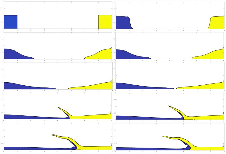
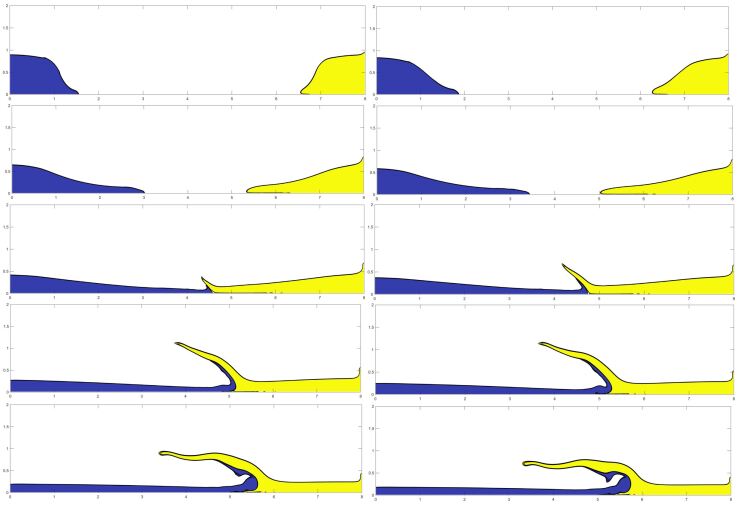
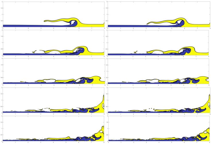
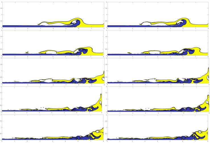
Figure 20: Evolution of the three phases in the three-phase dam break problem. From left to right, top to bottom, $t$ is 0.00, 0.50, 0.75, 1.00, …, 10.00. Blue: Water, Yellow: Oil, and White: Air.

5.2.5 Three-phase rising bubbles with moving contact lines

We consider a three-phase rising bubble problem with moving contact lines, where an air (Phase 1) bubble is surrounded by an oil (Phase 2) drop, inside a water (Phase 3) tank. The buoyancy effect drives both the air bubble and the oil drop to move upward. After they touch the top wall of the water tank, contact lines between the fluids and the wall are formed and they begin to slide along the wall. The material properties of the fluids are listed in Table 6. Non-dimensionalization is performed based on a density scale $1.2041\mathrm{kg/m^{3}}$, a length scale $0.01\mathrm{m}$, and an acceleration scale $1\mathrm{m/s^{2}}$. After that, the domain considered is $[-0.5,0.5]\times[0,1.5]$ and its boundaries are all no-slip. We use $[100\times 150]$ cells to discretize the domain and the time step is $\Delta t=2.5\times 10^{-5}$. Initially, the flow is stationary. Both the air bubble and the oil drop are circular, whose centers are at $(0,0.5)$. Their radii are $0.15$ and $0.3$, respectively. We consider three different sets of the contact angles at the top wall, which are $\theta_{1,2}^{T}=\theta_{2,3}^{T}=\frac{\pi}{2}$ in the first case, $\theta_{1,2}^{T}=\frac{\pi}{2}$ and $\theta_{2,3}^{T}=\frac{2\pi}{3}$ in the second case, and $\theta_{1,2}^{T}=\frac{\pi}{6}$ and $\theta_{2,3}^{T}=\frac{2\pi}{3}$ in the last case. The evolution of the three phases in the three cases are shown in Fig.21, Fig.22, and Fig.23, respectively, up to $t=2.5$.

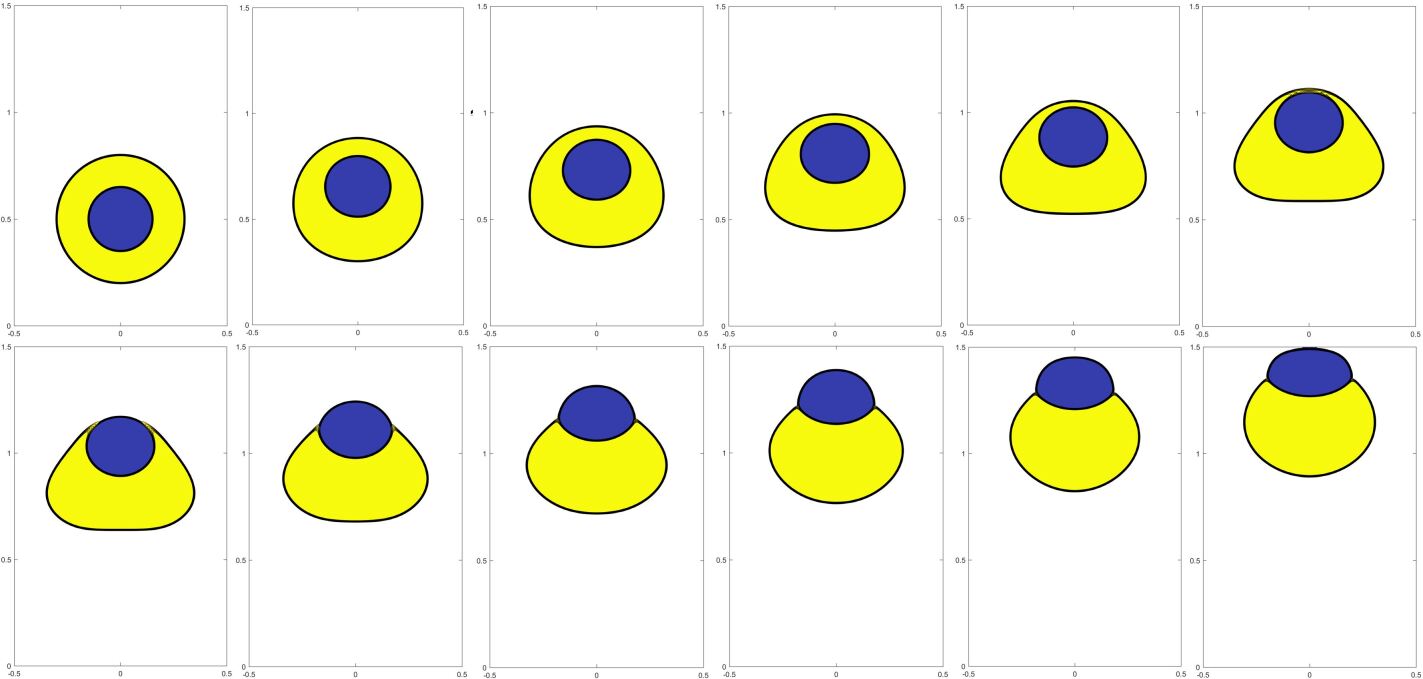
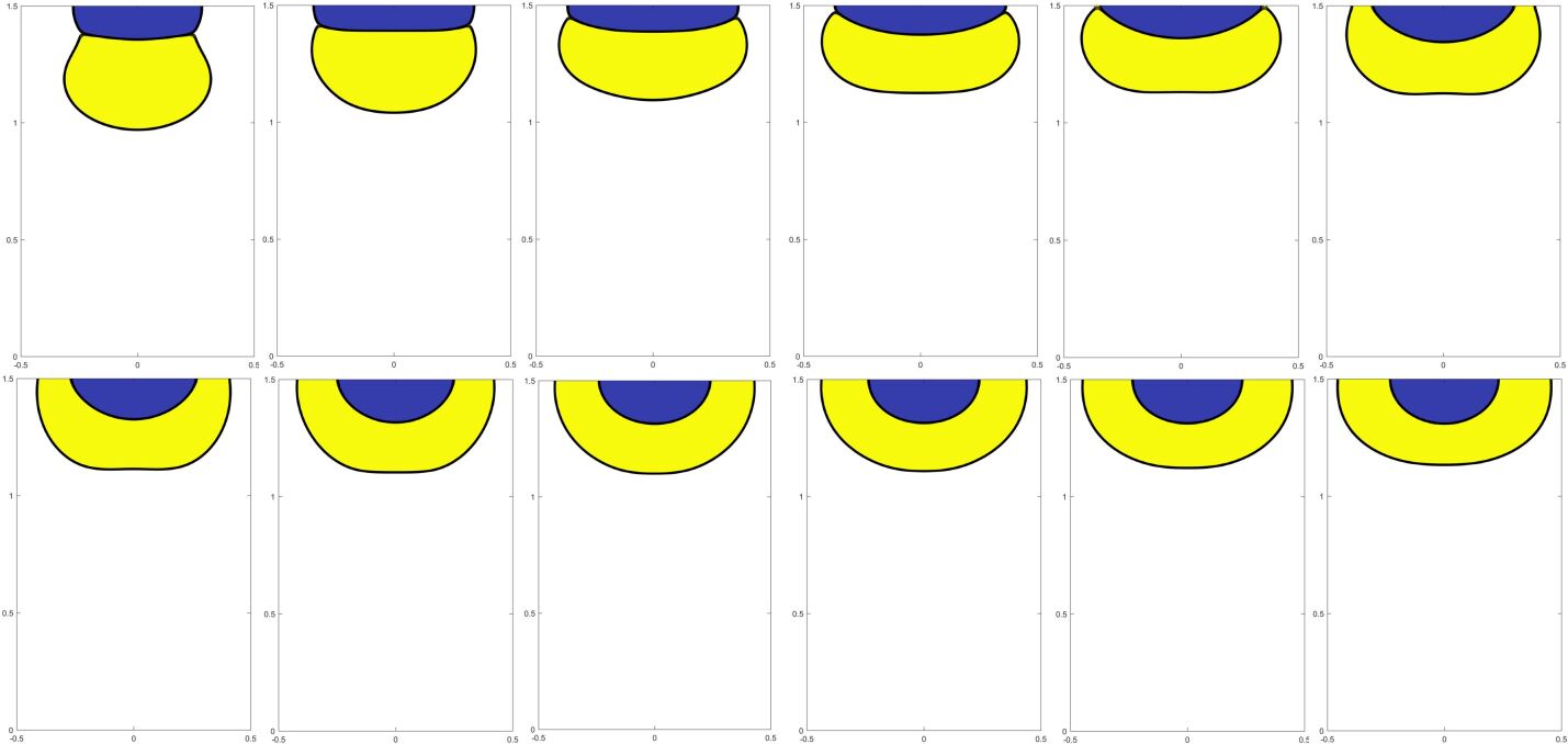
Figure 21: Evolution of the three phases in the three-phase rising bubble with moving contact lines, where $\theta_{1,2}^{T}=\frac{\pi}{2}$ and $\theta_{2,3}^{T}=\frac{\pi}{2}$. From left to right, top to bottom, $t$ is 0.00, 0.3, 0.4, 0.5, …, 2.5. Blue: Air (Phase 1), Yellow: Oil (Phase 2), and White: Water (Phase 3).

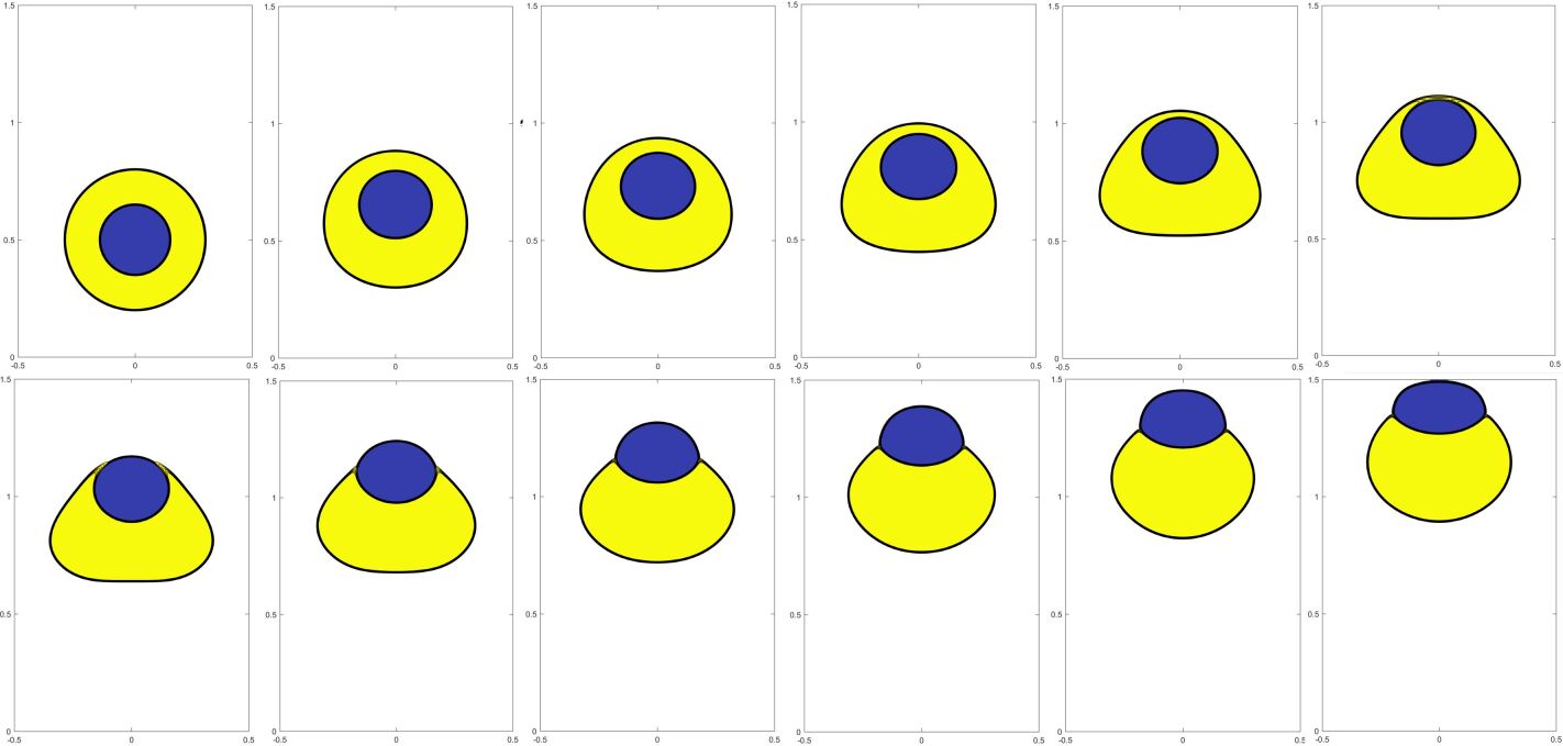
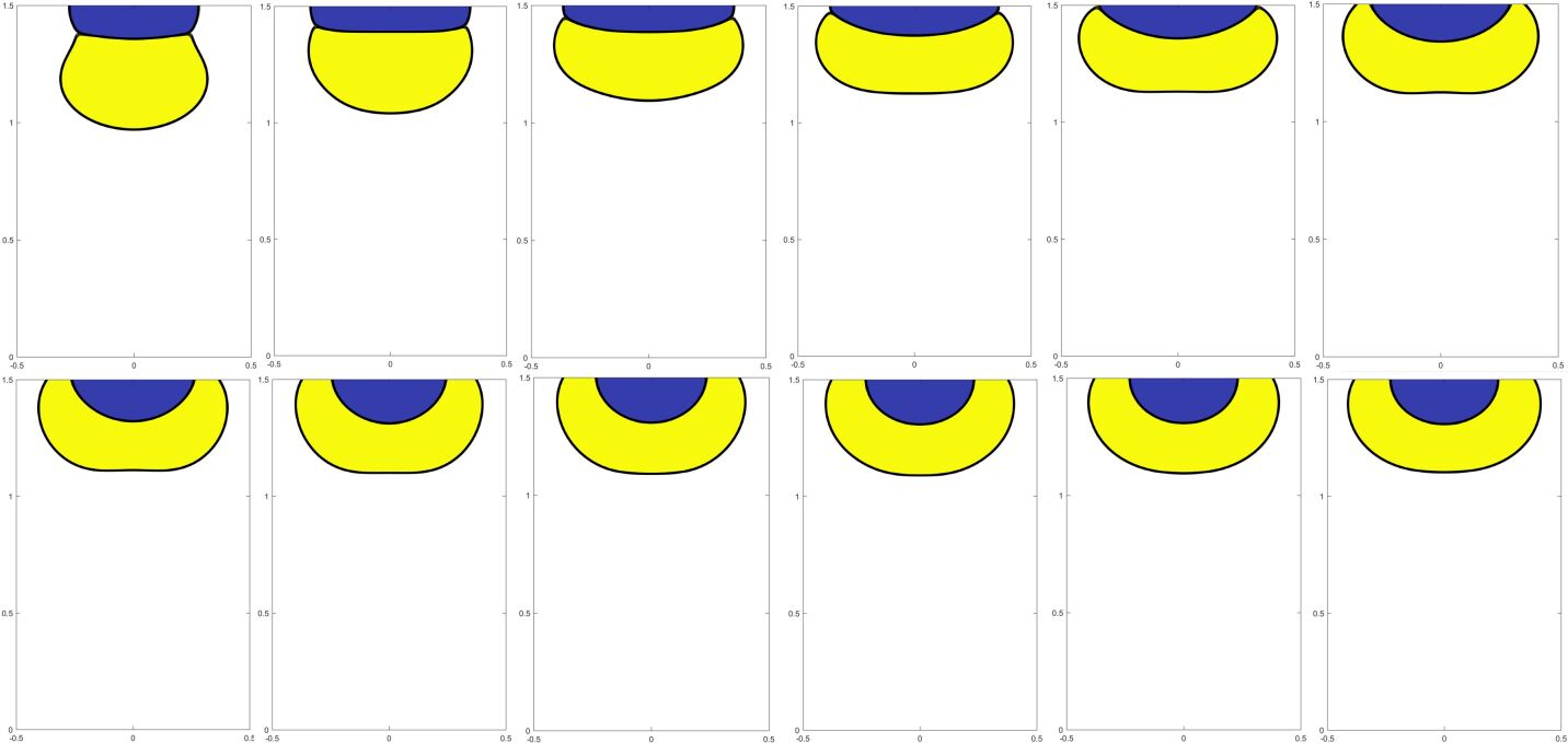
Figure 22: Evolution of the three phases in the three-phase rising bubble with moving contact lines, where $\theta_{1,2}^{T}=\frac{\pi}{2}$ and $\theta_{2,3}^{T}=\frac{2\pi}{3}$. From left to right, top to bottom, $t$ is 0.00, 0.3, 0.4, 0.5, …, 2.5. Blue: Air (Phase 1), Yellow: Oil (Phase 2), and White: Water (Phase 3).

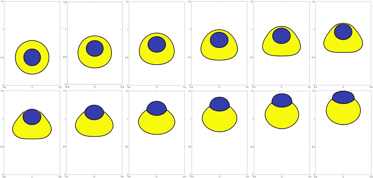
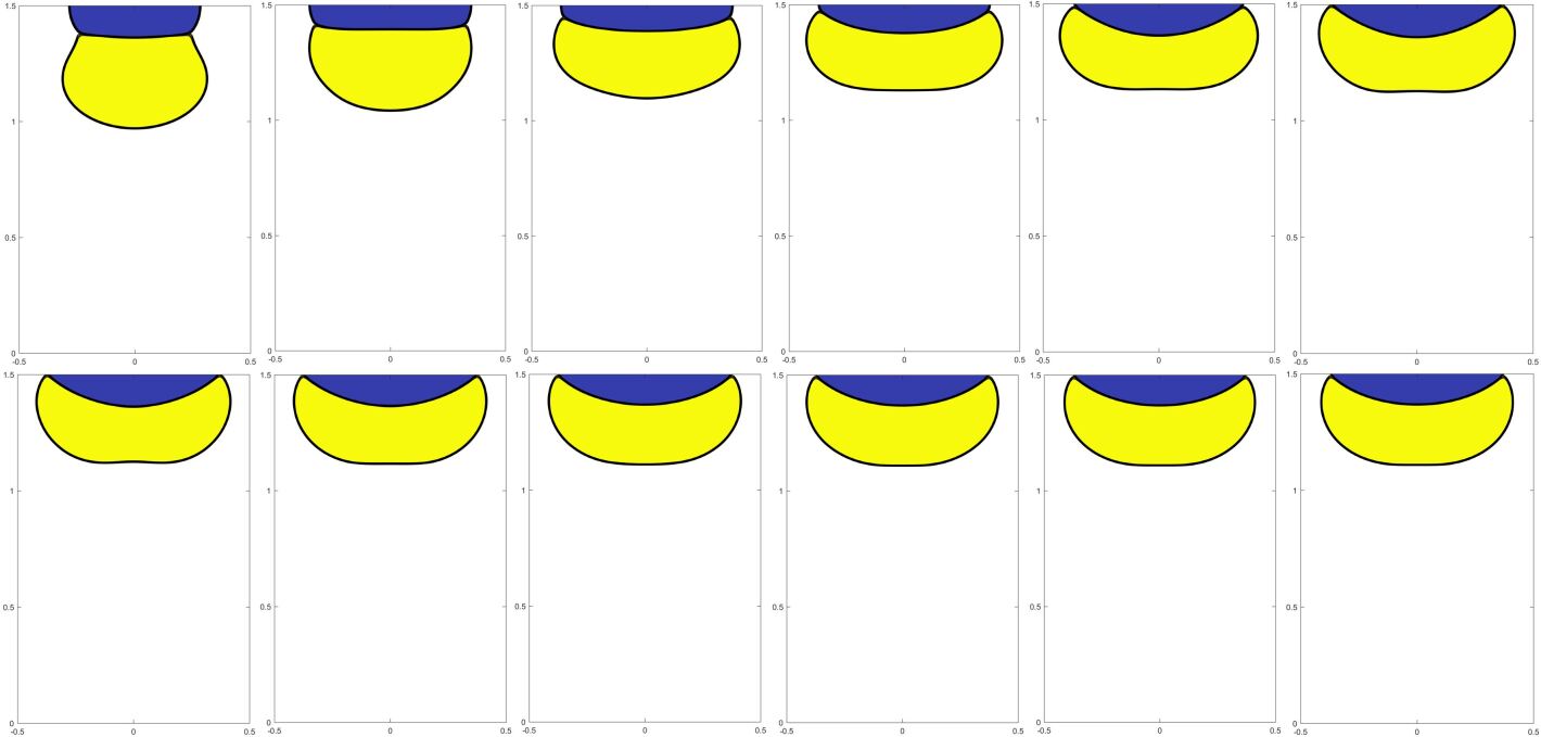
Figure 23: Evolution of the three phases in the three-phase rising bubble with moving contact lines, where $\theta_{1,2}^{T}=\frac{\pi}{6}$ and $\theta_{2,3}^{T}=\frac{2\pi}{3}$. From left to right, top to bottom, $t$ is 0.00, 0.3, 0.4, 0.5, …, 2.5. Blue: Air (Phase 1), Yellow: Oil (Phase 2), and White: Water (Phase 3).

There is no significant difference among Fig.21, Fig.22, and Fig.23 before $t=1.8$. This is expected since the contact angle boundary condition should only influence the dynamics close to the top wall. At the beginning, the air bubble moves upward, relative to the oil drop, driven by the buoyancy effect. The drag introduced by the relative motion between the air bubble and the oil drop, along with the buoyancy effect between the oil and the water, drives the oil drop moving upward. Since the density contrast between the air and the oil is much larger than that between the water and the oil, the motion of the air bubble is more pronounced, and as a result, the air bubble crosses the water-oil interface. After that, the triple points between the air, oil, and water is formed, and the three phases gradually reach an equilibrium configuration. This equilibrium configuration keeps moving upward without observable deformation until the air bubble touches the top wall. After touching the top wall, the air bubble quickly spreads along the top wall and is further compressed along the vertical direction because of the rising motion of the oil drop. The difference among the three cases begins with the oil drop touching the top wall, i.e., right after $t=1.8$, since the contact angle between the water and oil at the top wall varies from case to case. In Fig.21 and Fig.22, the spreading length of the oil drop is larger than that of the air bubble, and the compressed air bubble is relaxed to a shape close to a semi circle. In Fig.23, the spreading length of the oil drop is very close to that of the air bubble, and the relaxation of the air bubble is not obvious. Finally, both the air bubble and the oil drop stay at the top wall with the assigned contact angles.

6 Conclusions

In the present study, we develop a consistent and conservative Phase-Field method, including both the model and scheme, for the multiphase flows where there can be an arbitrary number of incompressible and immiscible phases.

The first important question answered is how to physically couple a mass conservative Phase-Field equation to the hydrodynamics. The consistency of mass conservation and the consistency of mass and momentum transport are implemented, based on a generic multiphase Phase-Field equation, to obtain the “actural” mass conservation equation and the consistent mass flux of the multiphase flow model, which can be different from the sharp-interface one particularly with a divergence-free velocity, and then the momentum equation that is compatible with the “actual” mass conservation equation and in general different from the Navier-Stokes equation. The direct consequence of satisfying these two consistency conditions is that the resulting momentum equation satisfies the Galilean invariance and implies the conservation of kinetic energy, which is independent of the Phase-Field equation. We further illustrate that the consistency of mass conservation and the consistency of mass and momentum transport produce the “optimal” coupling in the sense that failures of satisfying the second law of thermodynamics or the consistency of reduction of the multiphase flow model only result from the same failures of the Phase-Field equation but are not contributed by the newly obtained momentum equation from those two consistency conditions. The consistency conditions as well as the formulations derived from them can be physically explained using the control volume analysis and mixture theory. Moreover, those consistency conditions are valid to alternative mutliphase flow models whose velocity can be non-divergence-free, and the general formulations independent of the interpretation of the velocity are summarized. Specifically in the present study, we choose the Phase-Field equation in (Dong2018, ) to complete the present consistent and conservative multiphase flow model because it is fully reduction consistent, although the developed theory and formulations are directly applicable to other existing Phase-Field equations. The present multiphase flow model conserves the mass and momentum and assures the summation of the volume fractions to be unity, in addition to satisfying the consistency conditions mentioned.

Several novel numerical techniques are developed, which helps to preserve the physical properties of the multiphase flow model and therefore avoids unphysical behaviors due to numerical approximation. The gradient-based phase selection procedure is developed to address the issue of producing fictitious phases, local voids, or overfilling in the multiphase flows by the discretized convection term, and this procedure admits any numerical method to compute the convection flux. The balanced-force method and the conservative method are proposed to discretize the surface force, and the conservative method is a general mulitphase interfacial tension model that contributes to the discrete conservation of momentum. The general theorems are developed to address the difficulty of preserving the consistency conditions on the discrete level, and therefore discretely reproduce the physical coupling between the Phase-Field and momentum equations. Those theorems have no restrictions on the number of phases, the form of the Phase-Field equation, or the numerical scheme to solve the Phase-Field equation. They illustrate that the numerical operations in the fully discrete Phase-Field and momentum equations are not independent.

A consistent and conservative scheme is developed for the present multiphase flow model, based on the schemes in (Dong2018, ; Huangetal2020, ) for the Phase-Field and momentum equations, respectively, and with the help of the novel numerical techniques. The physical properties of the scheme are carefully analyzed, which were not performed in (Dong2018, ; Huangetal2020, ) or other works. The scheme is consistent because it satisfies the consistency of mass conservation, consistency of mass and momentum transport, and consistency of reduction. As a result, it solves advection (or translation) problems exactly regardless of the number, the material properties, or the interface shapes of the phases, eliminates the production of fictitious phases, and discretely recovers the single-phase Navier-Stokes dynamics in each bulk-phase region. The scheme is conservative, because it conserves the order parameters and therefore the mass of each phase and the mass of the fluid mixture, and the momentum if the surface force is either neglected or computed conservatively, e.g., using the newly developed conservative method. Besides, the scheme guarantees the summation of the volume fractions to be unity at every grid point so that no voids or overfilling are produced.

A series of numerical experiments are performed to validate all the aforementioned properties of the scheme, and the numerical results are consistent with our analyses. In addition, we observe the convergence of the numerical solution of the present multiphase flow model from the developed scheme to the sharp-interface solution with a rate between 1.5th- and 2nd-order, no matter whether the balanced-force or conservative method for the surface force is used. In the steady drop problem, the balanced-force method gives a smaller spurious current and faster convergence rate than the conservative method. As illustrated in the large-density-ratio advection problem, violating the consistency conditions results in unphysical velocity fluctuations and interface deformations and finally triggers numerical instability, while the physical result is well reproduced by our scheme even with an extremely large density ratio. In the horizontal shear layer problem, we demonstrate the generation of fictitious phases, local voids, or overfilling when the gradient-based phase selection procedure does not implemented. These unphysical behaviors disappear after the procedure is activated. Different from using the conservative method, the momentum is only essentially conserved with the balanced-force method, and the non-conservation is very small and is reduced after grid refinement. Although it is not shown in the analyses, our numerical results reproduce the behaviors of the energy law of the present multiphase flow model, i.e., Eq.(22). The conservative method performs better in the inviscid case when the grid is coarse, while the difference between the two methods is not significant in the fine-grid solution or in the case including viscosity. Therefore, both the balanced-force method and the conservative method are practical and effective for the multiphase flows. Various realistic multiphase flow problems are performed to verify and demonstrate the capability of the present multiphase flow model and scheme. The numerical results agree well with the exact/asymptotic solutions, other numerical results, and experimental measurements, in problems having significant density and/or viscosity ratios. The multiphase interface configuration is far more complicated than the two-phase one due to strong interactions among different phases in the long-time dynamics.

It is worth mentioning that all the analyses, theorems, and formulations in the present study are valid for an arbitrary number of phases and dimensions, although some of them are reported in two dimensions for a clear presentation. In summary, strong interactions among different phases produce complicated dynamics. Implementing the consistency conditions provides a practical and convenient way to directly obtain physical “mixture-level” models for the multiphase problems. The proposed scheme for the present multiphase flow model preserves many physical properties of the multiphase flows in a discrete sense. It is robust, accurate, and applicable to study various multiphase flows even when there are large differences of material properties.

Appendix

Equilibrium solution of the floating liquid lens

At the equilibrium state, the free energy of the floating lens is minimized. In other words, the area (or the length in 2D) of the interface of the drop should be minimized under the mass conservation (or the area constraint in 2D), the force balance at the triple points, and the normal stress balance at the interfaces. As a result, in 2D, the equilibrium shape of the drop is a combination of two circular segments, which satisfies the aforementioned constraints. As illustrated in Fig.24, the drop, called Phase 2, has an initial radius $R_{0}$. The interfacial tensions between Phases 1 and 2, Phases 1 and 3, and Phases 2 and 3 are $\sigma_{1,2}$, $\sigma_{1,3}$, and $\sigma_{2,3}$, respectively. When the drop reaches its equilibrium shape, the radius of the upper circular segment is $R_{2,3}$ and the angle between the circular segment and the horizontal line is $\theta_{2,3}$, while they are denoted by $R_{1,2}$ and $\theta_{1,2}$ for the lower circular segment.

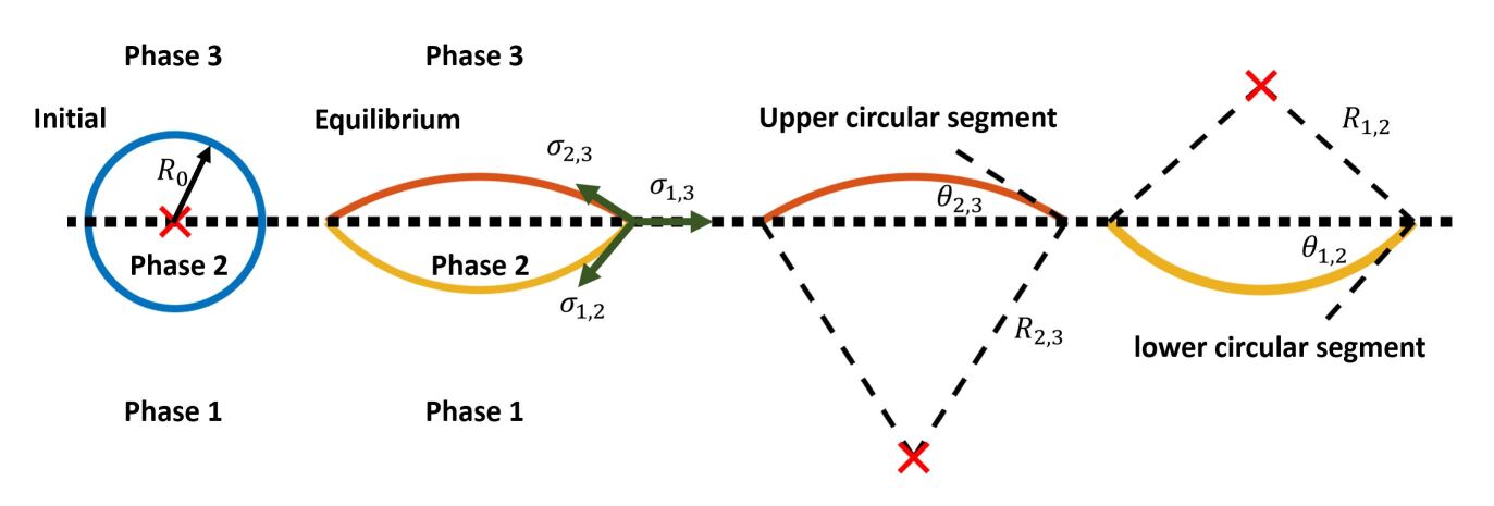
Figure 24: Schematic of a floating liquid lens.

First, we consider the force balance at the triple points, which are

$$\sigma_{2,3}\cos(\theta_{2,3})+\sigma_{1,2}\cos(\theta_{1,2})=\sigma_{1,3}$$ (69)

$$\sigma_{2,3}\sin(\theta_{2,3})=\sigma_{1,2}\sin(\theta_{1,2}),$$

and its solutions for $\theta_{1,2}$ and $\theta_{2,3}$ are

$$\theta_{1,2}=\cos^{-1}\left(\frac{\sigma_{1,3}^{2}+\sigma_{1,2}^{2}-\sigma_{2,3}^{2}}{2\sigma_{1,2}\sigma_{1,3}}\right),$$ (70)

$$\theta_{2,3}=\sin^{-1}\left(\frac{\sigma_{1,2}}{\sigma_{2,3}}\sin(\theta_{1,2})\right).$$

Second, we can compute the areas of the two circular segments as

$$S_{1,2}=R_{1,2}^{2}\left(\theta_{1,2}-\sin(\theta_{1,2})\cos(\theta_{1,2})\right)$$ (71)

$$S_{2,3}=R_{2,3}^{2}\left(\theta_{2,3}-\sin(\theta_{2,3})\cos(\theta_{2,3})\right).$$

The area constraint requires that

$$S_{1,2}+S_{2,3}=\pi R_{0}^{2}.$$ (72)

Third, the normal stress balances at the upper and lower circular segments are considered. By applying the Young-Laplace Law at the two circular segments, we have

$$\frac{\sigma_{1,2}}{R_{1,2}}=p_{1,2}=p_{drop}=p_{2,3}=\frac{\sigma_{2,3}}{R_{2,3}},$$ (73)

where $p_{1,2}$ is the pressure inside the drop and right beside the lower circular segment, $p_{2,3}$ is the pressure inside the drop and right beside the upper circular segment, and $p_{drop}$ is the pressure inside the drop. By combining the area constraint and the normal stress balances, $R_{1,2}$ and $R_{2,3}$ are obtained, i.e.,

$$R_{2,3}=R_{0}\sqrt{\frac{\pi}{(\theta_{2,3}-\sin(\theta_{2,3})\cos(\theta_{2,3}))+(\frac{\sigma_{1,2}}{\sigma_{2,3}})^{2}(\theta_{1,2}-\sin(\theta_{1,2})\cos(\theta_{1,2}))}}$$ (74)

$$R_{1,2}=R_{2,3}\frac{\sigma_{1,2}}{\sigma_{2,3}}.$$

Finally, it’s straightforward to obtain the equilibrium thickness of the drop,

$$e_{d}=R_{2,3}\left(1-\cos(\theta_{2,3})\right)+R_{1,2}\left(1-\cos(\theta_{1,2})\right)$$ (75)

Equilibrium solution of a drop on a homogeneous flat surface

At the equilibrium state, the free energy of a drop placed on a homogeneous surface is minimized. In other words, the area (or the length in 2D) of the interface of the drop should be minimized under the mass conservation (or the area constraint in 2D) and the contact angle constraint. As a result, in 2D, the equilibrium shape of the drop is a circular segment, which intersects the homogeneous flat surface with the given contact angle, and the enclosed area is the same as the initial one. As illustrated in Fig.25, the area enclosed by the circular segment is

$$S_{d}=R_{d}^{2}\left(\theta_{s}-\sin(\theta_{s})\cos(\theta_{s})\right),$$ (76)

where $R_{d}$ is the radius of the circular segment and $\theta_{s}$ is the contact angle between the drop and the surface. The area constraint requires that $S_{d}=\frac{\pi}{2}R_{0}^{2}$, where $R_{0}$ is the radius of the initial semi-circular drop. Thus, we can obtain

$$R_{d}=R_{0}\sqrt{\frac{\pi/2}{\theta_{s}-\sin(\theta_{s})\cos(\theta_{s})}}.$$ (77)

Once $R_{d}$ is found by given $R_{0}$ and $\theta_{s}$, the height and the spreading length of the equilibrium drop can be computed as

$$H_{d}=R_{d}\left(1-\cos(\theta_{s})\right),$$ (78)

$$L_{d}=2R_{d}\sin(\theta_{s}).$$ (79)

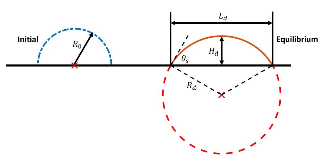
Figure 25: Schematic of a drop on a homogeneous flat surface.

References

- [1] H. Abels, H. Garcke, and G. Grun. Thermodynamically consistent, frame indifferent diffuse interface models for incompressible two-phase flows with different densities. Mathematical Models and Methods in Applied Sciences, 22:1150013, 2012.
- [2] S. Achanta, J.H. Cushman, and M.R. Okos. On multicomponent, multiphase thermomechanics with interfaces. International Journal of Engineering Science, 32(11):1717–1738, 1994.
- [3] H.A. Akhlaghi Amiri and A.A. Hamouda. Evaluation of level set and phase field methods in modeling two phase flow with viscosity contrast through dual-permeability porous medium. International Journal of Multiphase Flow, 52:22–34, 2013.
- [4] D.M. Anderson, G.B. McFadden, and A.A. Wheeler. Diffuse-interface methods in fluid mechanics. Annu. Rev. Fluid Mech., 30:139–165, 1998.
- [5] L.S. Bennethum and J.H. Cushman. Multicomponent, multiphase thermodynamics of swelling porous media with electroquasistatics: Ii. constitutive theory. Transport in Porous Media, 47(3):337–362, 2002.
- [6] M. Boger, J. Schlottke, C.D. Munz, and B. Weigand. Reduction of parasitic currents in the dns vof code fs3d. In 12th Workshop on Two-Phase Flow Predictions, 2010.
- [7] R.M. Bowen. Theory of Mixtures, Part I. Continuum Physics. Academic Press, New York, eringen, a.c. edition, 1976.
- [8] F. Boyer and C. Lapuerta. Study of a three component cahn-hilliard flow model. ESAIM: Mathematical Modelling and Numerical Analysis, 40(4):653–687, 2006.
- [9] F. Boyer, C. Lapuerta, S. Minjeaud, B. Piar, and M. Quintard. Cahn-hilliard/navier-stokes model for the simulation of three-phase flows. Transport in Porous Media, 82(3):463–483, 2010.
- [10] F. Boyer and S. Minjeaud. Hierarchy of consistent n-component cahn–hilliard systems. Math. Models Methods Appl. Sci., 24:2885–2928, 2014.
- [11] J.U. Brackbill, D.B. Kothe, and C. Zemach. A continuum method for modeling surface tension. J. Comput. Phys., 100:335–354, 1992.
- [12] M. Brassel and E. Bretin. A modified phase field approximation for mean curvature flow with conservation of the volume. Math. Methods Appl. Sci., 34:1157–1180, 2011.
- [13] M. Bussmann, D.B. Kothe, and J.M. Sicilian. Modeling high density ratio incompressible interfacial flows. In Proceedings of the ASME 2002 Joint U.S.-European Fluids Engineering Division Conference, Volume 1: Fora, Parts A and B. Montreal, Quebec, Canada. July 14–18, 2002, pages 707–713. ASME, 2002.
- [14] V.L. Chenadec and H. Pitsch. A monotonicity preserving conservative sharp interface flow solver for high density ratio two-phase flows. J. Comput. Phys., 249:185–203, 2013.
- [15] R. Chiodi and O. Desjardins. A reformulation of the conservative level set reinitialization equation for accurate and robust simulation of complex multiphase flows. J. Comput. Phys., 343:186–200, 2017.
- [16] P-G de Gennes, F. Brochard-Wyart, and D. Quere. Capillarity and Wetting Phenomena. Springer, 2003.
- [17] H. Ding, P.D.M. Spelt, and C. Shu. Diffuse interface model for incompressible two-phase flows with large density ratios. J. Comput. Phys., 226:2078–2095, 2007.
- [18] S. Dong. An efficient algorithm for incompressible n-phase flows. J. Comput. Phys., 276:691–728, 2014.
- [19] S. Dong. Physical formulation and numerical algorithm for simulating n immiscible incompressible fluids involving general order parameters. J. Comput. Phys., 836:98–128, 2015.
- [20] S. Dong. Wall-bounded multiphase flows of n immiscible incompressible fluids: Consistency and contact-angle boundary condition. J. Comput. Phys., 338:21–67, 2017.
- [21] S. Dong. Multiphase flows of n immiscible incompressible fluids: A reduction-consistent and thermodynamically-consistent formulation and associated algorithm. J. Comput. Phys., 361:1–49, 2018.
- [22] S. Dong and J. Shen. A time-stepping scheme involving constant coefficient matrices for phase-field simulations of two-phase incompressible flows with large density ratios. J. Comput. Phys., 231:5788–5804, 2012.
- [23] D.A. Drew. Mathematical modeling of two-phase flow. Annual review of fluid mechanics, 15(1):261–291, 1983.
- [24] R.P. Fedkiw, T. Aslam, B. Merriman, and S. Osher. A non-oscillatory eulerian approach to interfaces in multimaterial flows (the ghost fluid method). J. Comput. Phys., 152:457–492, 1999.
- [25] J. H. Ferziger and M. Perić. Computational Methods for Fluid Dynamics. Springer, 3 edition, 2002.
- [26] M.M. Francois. Recent numerical and algorithmic advances within the volume tracking framework for modeling interfacial flows. Procedia IUTAM, 15:270–277, 2015.
- [27] M.M. Francois, J.S. Cummins, E.D. Dendy, D.B. Kothe, M.J. Sicilian, and W.W. Williams. A balanced-force algorithm for continuous and sharp interfacial surface tension models within a volume tracking framework. J. Comput. Phys., 213:141–173, 2006.
- [28] F. Gibou, R. Fedkiw, and S. Osher. A review of level-set methods and some recent applications. J. Comput. Phys., 353:82–109, 2018.
- [29] W.G. Gray and S.M. Hassanizadeh. Unsaturated flow theory including interfacial phenomena. Water Resources Research, 27(8):1855–1863, 1991.
- [30] J.L. Guermond and L. Quartapelle. A projection fem for variable density incompressible flows. J. Comput. Phys., 165:167–188, 2000.
- [31] Z. Guo and P. Lin. A thermodynamically consistent phase-field model for two-phase flows with thermocapillary effects. Journal of Fluid Mechanics, 766:226–271, 2015.
- [32] C.W. Hirt and B.D. Nichols. Volume of fluid (vof) method for the dynamics of free boundaries. J. Comput. Phys., 39:201–225, 1981.
- [33] Z. Huang, G. Lin, and A.M. Ardekani. A mixed upwind/central weno scheme for incompressible two-phase flows. J. Comput. Phys., 387:455–480, 2019.
- [34] Z. Huang, G. Lin, and A.M. Ardekani. Consistent and conservative scheme for incompressible two-phase flows using the conservative allen-cahn model. J. Comput. Phys., 420:109718, 2020.
- [35] Z. Huang, G. Lin, and A.M. Ardekani. Consistent, essentially conservative and balanced-force phase-field method to model incompressible two-phase flows. J. Comput. Phys., 406:109192, 2020.
- [36] Z. Huang, G. Lin, and A.M. Ardekani. A consistent and conservative volume distribution algorithm and its applications to multiphase flows using phase-field models. International Journal of Multiphase Flow, 142:103727, 2021.
- [37] S. Hysing, S. Turek, D. Kuzmin, N. Parolini, E. Burman, S. Ganesan, and L. Tobiska. Quantitative benchmark computations of two-dimensional bubble dynamics. Int. J. Numer. Methods. Fluids, 60:1259–1288, 2009.
- [38] Satoshi Ii, Kazuyasu Sugiyama, Shintaro Takeuchi, Shu Takagi, Yoichiro Matsumoto, and Feng Xiao. An interface capturing method with a continuous function: The thinc method with multi-dimensional reconstruction. J. Comput. Phys., 231(5):2328–2358, 2012.
- [39] D. Jacqmin. Calculation of two-phase navier-stokes flows using phase-field modeling. J. Comput. Phys., 155:96–127, 1999.
- [40] D. Jamet, D. Torres, and J.U. Brackbill. On the theory and computation of surface tension: The elimination of parasitic currents through energy conservation in the second-gradient method. J. Comput. Phys., 182:262–276, 2002.
- [41] G-S Jiang and C-W Shu. Efficient implementation of weighted eno schemes. J. Comput. Phys., 126:202–228, 1996.
- [42] J. Kim. Phase field computations for ternary fluid flows. Comput. Methods Appl. Mech. Engre., 196:4779–4788, 2007.
- [43] J. Kim. A generalized continuous surface tension force formulation for phase-field models for multi-component immiscible fluid flows. Comput. Methods Appl. Mech. Engre., 198:3105–3112, 2009.
- [44] J. Kim. Phase-field models for multi-component fluid flows. Commun. Comput. Phys., 12:613–661, 2012.
- [45] J. Kim and H.G. Lee. A new conservative vector-valued allen-cahn equation and its fast numerical method. Comput. Phys. Commun., 221:102–108, 2017.
- [46] J. Kim and J. Lowengrub. Phase field modeling and simulation of three-phase flows. Interfaces Free Bound., 7:435–466, 2005.
- [47] S. Kim. A continuous surface tension force formulation for diffuse-interface models. J. Comput. Phys., 204:784–804, 2005.
- [48] B. Lalanne, L.R. Villegas, S. Tanguy, and F. Risso. On the computation of viscous terms for incompressible two-phase flows with level set/ghost fluid method. J. Comput. Phys., 301:289–307, 2015.
- [49] I. Langmuir. Oil lenses on water and the nature of monomolecular expanded films. J. Chem. Phys., 1:756–776, 1933.
- [50] L. Leal. Advanced Transport Phenomena: Fluid Mechanics and Convective Transport Processes. Cambridge University Press, 2007.
- [51] H.G. Lee and J. Kim. An efficient numerical method for simulating multiphase flows using a diffuse interface model. Physica A, 423:33–50, 2015.
- [52] J. Li and Q. Wang. A class of conservative phase field models for multiphase fluid flows. Journal of Applied Mechanics, 81(2):021004, 2014.
- [53] Frank Losasso, Tamar Shinar, Andrew Selle, and Ronald Fedkiw. Multiple interacting liquids. In ACM Transactions on Graphics (TOG), volume 25, pages 812–819. ACM, 2006.
- [54] John Lowengrub and Lev Truskinovsky. Quasi-incompressible cahn-hilliard fluids and topological transitions. Proceedings of the Royal Society of London. Series A: Mathematical, Physical and Engineering Sciences, 454(1978):2617–2654, 1998.
- [55] J.C. Martin and W.J. Moyce. An experimental study of the collapse of liquid columns on a rigid horizontal plane. Philosophical Transactions of the Royal Society of London, Series A, 244:312–324, 1952.
- [56] S. Mirjalili, C.B. Ivey, and A. Mani. Comparison between the diffuse interface and volume of fluid methods for simulating two-phase flows. Int. J. Multiph. Flow, 116:221–238, 2019.
- [57] Seyedshahabaddin Mirjalili. A novel diffuse interface method for two-phase flows and application in simulation of micro-bubble entrainment. PhD thesis, Stanford University, 2019.
- [58] Y. Morinishi, T.S. Lund, O.V. Vasilyev, and P. Moin. Fully conservative higher order finite difference schemes for incompressible flow. J. Comput. Phys., 143:90–124, 1998.
- [59] N. Nangia, E.G. Boyce, N.A. Patankar, and A.P.S. Bhalla. A robust incompressible navier-stokes solver for high density ratio multiphase flows. J. Comput. Phys., 390:548–594, 2019.
- [60] J.T. Oden, A. Hawkins, and S. Prudhomme. General diffuse-interface theories and an approach to predictive tumor growth modeling. Mathematical Models and Methods in Applied Sciences, 20(03):477–517, 2010.
- [61] E. Olsson and G. Kreiss. A conservative level set method for two phase flow. J. Comput. Phys., 210:225–246, 2005.
- [62] E. Olsson, G. Kreiss, and S. Zahedi. A conservative level set method for two phase flow ii. J. Comput. Phys., 225:785–807, 2007.
- [63] S. Osher and A.J. Sethian. Fronts propagating with curvature-dependent speed: Algorithms based on hamilton-jacobi formulations. J. Comput. Phys., 79:12–49, 1988.
- [64] M. Owkes and O. Desjardins. A mass and momentum conserving unsplit semi-lagrangian framework for simulating multiphase flows. J. Comput. Phys., 332:21–46, 2017.
- [65] A. Pathak and M. Raessi. A three-dimensional volume-of-fluid method for reconstructing and advecting three-material interfaces forming contact lines. J. Comput. Phys., 307:550–573, 2016.
- [66] S. Popinet. An accurate adaptive solver for surface-tension-driven interfacial flows. J. Comput. Phys., 228:5838–5866, 2009.
- [67] S. Popinet. Numerical models for surface tension. Annu. Rev. Fluid Mech., 50:49–75, 2018.
- [68] A. Prosperetti and G. Tryggvason. Computational Methods for Multiphase Flow. Cambridge University Press, 2007.
- [69] L. Qian, Y. Wei, and F. Xiao. Coupled thinc and level set method: A conservative interface capturing scheme with high-order surface representations. J. Comput. Phys., 373:284–303, 2018.
- [70] M. Raessi and H. Pitsch. Consistent mass and momentum transport for simulating incompressible interfacial flows with large density ratios using the level set method. Comput. Fluids, 63:70–81, 2012.
- [71] Abadi R.H.H., M.H. Rahimian, and A. Fakhari. Conservative phase-field lattice-boltzmann model for ternary fluids. J. Comput. Phys., 374:668–691, 2018.
- [72] C.M. Rhie and W.L. Chow. A numerical study of the turbulent flow past an isolated airfoil with trailing edge separation. In AIAA/ASME 3rd Joint Thermophysics, Fluids, Plasma and Heat Transfer Conference, pages AIAA–82–0998, 1982.
- [73] J. Rubinstein and P. Sternberg. Nonlocal reaction—diffusion equations and nucleation. IMA Journal of Applied Mathematics, 48(3):249–264, 1992.
- [74] M. Rudman. A volume-tracking method for incompressible multifluid flows with large density variations. Int. J. Numer. Methods. Fluids, 28:357–378, 1998.
- [75] R. Scardovelli and S. Zaleski. Direct numerical simulation of free-surface and interfacial flow. Annu. Rev. Fluid Mech., 31:567–603, 1999.
- [76] S.P. Schofield, R.V. Garimella, M.M. Francois, and R. Loubere. A second-order accurate material-order-independent interface reconstruction technique for multi-material flow simulations. J. Comput. Phys., 228:731–745, 2009.
- [77] S.P. Schofield, Christon M.A., V. Dyadechko, R.V. Garimella, R.B. Lowrie, and B.K. Swartz. Multi-material incompressible flow simulation using the moment-of-fluid method. Int. J. Numer. Meth. Fluids, 63:931–952, 2010.
- [78] J.A. Sethian and P. Smereka. Level set method for fluid interfaces. Annu. Rev. Fluid Mech., 35:341–372, 2003.
- [79] J Shen. Modeling and numerical approximation of two-phase incompressible flows by a phase-field approach. Multiscale Modeling and Analysis for Materials Simulation, 22:147–195, 2011.
- [80] Jie Shen, Xiaofeng Yang, and Qi Wang. Mass and volume conservation in phase field models for binary fluids. Communications in Computational Physics, 13(4):1045–1065, 2013.
- [81] L. Shen, H. Huang, P. Lin, Z. Song, and S. Xu. An energy stable c0 finite element scheme for a quasi-incompressible phase-field model of moving contact line with variable density. Journal of Computational Physics, 405:109179, 2020.
- [82] K.A. Smith, F.J. Solis, and D.L. Chopp. A projection method for motion of triple junctions by level sets. Interfaces Free Bound., 4:263–276, 2002.
- [83] D.P. Starinshak, S. Karni, and P.L. Roe. A new level set model for multimaterial flows. Interface and free boundaries, 4:263–276, 2002.
- [84] Y. Sun and C. Beckermann. Diffuse interface modeling of two-phase flows based on averaging: mass and momentum equations. Physica D: Nonlinear Phenomena, 198(3-4):281–308, 2004.
- [85] M. Sussman, P. Smereka, and S. Osher. A level set approach for computing solutions to incompressible two-phase flow. J. Comput. Phys., 114:146–159, 1994.
- [86] J. Towns, T. Cockerill, M. Dahan, I. Foster, K. Gaither, A. Grimshaw, V. Hazlewood, S. Lathrop, D. Lifka, R. Roskies, J.R. Scott, and W.-D. Nancy. Xsede: accelerating scientific discovery. Comput. Sci. Eng., 16:62–74, 2014.
- [87] G. Tryggvason. Numerical simulations of the rayleigh-taylor instability. J. Comput. Phys., 75:253–282, 1988.
- [88] G. Tryggvason, B. Bunner, A. Esmaeeli, D. Juric, N. Al-Rawahi, W. Tauber, J. Han, S. Nas, and Y.J. Jan. A front-tracking method for the computations of multiphase flow. J. Comput. Phys., 169:708–759, 2001.
- [89] G. Tryggvason, R. Scardovelli, and S. Zaleski. Direct Numerical Simulations of Gas-Liquid Multiphase Flows. Cambridge University Press, 2011.
- [90] S.O. Unverdi and G. Tryggvason. A front-tracking method for viscous, incompressible, multi-fluid flows. J. Comput. Phys., 100:25–37, 1992.
- [91] S. Wu and J. Xu. Multiphase allen-cahn and cahn-hilliard models and their discretizations with the effect of pairwise surface tensions. J. Comput. Phys., 343:10–32, 2017.
- [92] F Xiao, Y Honma, and T Kono. A simple algebraic interface capturing scheme using hyperbolic tangent function. Int. J. Numer. Meth. Fluids, 48(9):1023–1040, 2005.
- [93] B. Xie and F. Xiao. Toward efficient and accurate interface capturing on arbitrary hybrid unstructured grids: The thinc method with quadratic surface representation and gaussian quadrature. J. Comput. Phys., 349:415–440, 2017.
- [94] K. Yokoi. A practical numerical framework for free surface flows based on clsvof method, multi-moment methods, and density-scaled csf model: Numerical simulations of droplet splashing. J. Comput. Phys., 232:252–271, 2013.
- [95] C.Y. Zhang, H. Ding, P. Gao, and Y.L. Wu. Diffuse interface simulation of ternary fluids in contact with solid. J. Comput. Phys., 309:37–51, 2016.
- [96] Q. Zhang and X.P. Wang. Phase field modeling and simulation of three-phase flow on solid surfaces. J. Comput. Phys., 319:79–107, 2016.