Evolution of the density PDF in star forming clouds: the role of gravity.

Abstract

We derive an analytical theory of the PDF of density fluctuations in supersonic turbulence in the presence of gravity in star-forming clouds. The theory is based on a rigorous derivation of a combination of the Navier-Stokes continuity equations for the fluid motions and the Poisson equation for the gravity. It extends upon previous approaches first by including gravity, second by considering the PDF as a dynamical system, not a stationary one. We derive the transport equations of the density PDF, characterize its evolution and determine the density threshold above which gravity strongly affects and eventually dominates the dynamics of turbulence. We demonstrate the occurence of two power law tails in the PDF, with two characteristic exponents, corresponding to two different stages in the balance between turbulence and gravity. Another important result of this study is to provide a procedure to relate the observed column density PDFs to the corresponding volume density PDFs. This allows to infer, from the observation of column-densities, various physical parameters characterizing molecular clouds, notably the virial parameter. Furthermore, the theory offers the possibility to date the clouds in units of ${t}_{\rm coll}$, the time since a statistically significant fraction of the cloud started to collapse. The theoretical results and diagnostics reproduce very well numerical simulations and observations of star-forming clouds. The theory provides a sound theoretical foundation and quantitative diagnostics to analyze observations or numerical simulations of star-forming regions and to characterize the evolution of the density PDF in various regions of molecular clouds.

1 Introduction

It has been established by many studies that the volume-weighted Probability Density Function (PDF) of supersonic isothermal turbulence displays a nearly lognormal shape for solenoidally driven turbulence, at least for Mach numbers ${\cal M}\lesssim 30$ (Vazquez-Semadeni 1994; Passot & Vázquez-Semadeni 1998; Kritsuk et al. 2007; Federrath et al. 2008, 2010; Pan et al. 2019a) even in the presence of magnetic fields (Lemaster & Stone 2008; Collins et al. 2012). In dense star-forming regions, however, the line-of-sight extinction and inferred column density PDFs have been observed to develop a power-law tail at high densities, for extinctions $A_{V}\gtrsim 2$-5 (e.g. Kainulainen et al. 2006, 2009; Schneider et al. 2012, 2013 and references therein), a feature identified as the signature of gravity. Indeed, a similar feature of the PDF is found in numerical simulations of turbulence that include self-gravity (e.g. Kritsuk et al. 2010; Ballesteros-Paredes et al. 2011; Cho & Kim 2011; Collins et al. 2012; Federrath & Klessen 2013; Lee et al. 2015; Burkhart et al. 2016).

Whereas these two opposite signatures of the PDF, lognormal vs power-law, seem to be clearly identified, when and how precisely gravity starts affecting the dynamics of turbulence and thus the properties and the evolution of the PDF remains to be fully understood. Understanding the statistical properties of supersonic turbulence is at the heart of analytical theories of the star formation process, so understanding the physics governing the shape and the evolution of the density PDF of supersonic turbulence is of prime importance. A few attempts have been made to explain the development of power law tails in the density PDF (Girichidis et al., 2014; Guszejnov et al., 2018; Donkov & Stefanov, 2018). These approaches, however, focus only on the gravitationally unstable parts of a cloud, using self-similar gravitational collapse models and/or geometrical arguments. While these models derive asymptotic exponents of power-law tails, they lack a complete description of the density fluctuations, both in the gravitationally stable and unstable parts of the cloud, and treat the PDF as a static system, even though Girichidis et al. (2014) follow numerically its time evolution. A first attempt to derive a robust theoretical framework of density fluctuations in compressible turbulence has been addressed by Pan et al. (2018, 2019a) based on the formalism developed by Pope (1981, 1985) and Pope & Ching (1993) for the PDF of any quantity, expressed as the conditional expectations of its time derivatives. Within the framework of this formalism, Pan et al. (2019a) used a probabilistic approach of turbulence to derive a theoretical formulation of the PDF of density fluctuations at steady state from first principles. In this paper, we follow a similar approach and derive an analytical theory to describe the dynamics of turbulence in dense regions of MCs and its interplay with gravity. The approach generalizes the aforementioned ones in two ways. First, we include the impact of gravity on the cloud’s dynamics. Second we consider the density PDF not as a stationary system but as a one evolving with time, implying that the conditional expectation of the flow velocity divergence is time-dependent and non zero. The theory explains the evolution of the PDF and determines the density thresholds above which gravity strongly affects and eventually dominates the dynamics of the turbulence. We provide a procedure to relate the observed column density PDFs to the underlying volume density PDFs, allowing to infer various physical parameters characterizing molecular clouds from observations. The theory and its diagnostics are confronted to numerical simulations of gravoturbulent collapsing clouds and to various available observations.

2 Mathematical Framework

2.1 Description of a molecular cloud

We consider an isolated, turbulent, self-gravitating molecular cloud. Neglecting for now the magnetic field, the cloud’s evolution is given by the standard Navier-Stokes and Poisson equations:

$$\frac{\partial\rho}{\partial t}+\bm{\nabla}\cdot\left(\rho\bm{v}\right) = 0,$$ (1)

$$\frac{\partial\bm{v}}{\partial t}+\left(\bm{v}\cdot\bm{\nabla}\right)\bm{v} = -\frac{1}{\rho}\bm{\nabla}P+\bm{\mathcal{G}}+\frac{1}{\rho}\bm{\nabla}\cdot\underline{\underline{\bm{\sigma}_{\nu}}},$$ (2)

$$\bm{\nabla}\cdot\bm{\mathcal{G}} = -4\pi G\rho,$$ (3)

where $\rho$ and $P$ denote respectively the density and pressure of the gas in the cloud, $\bm{v}$ the velocity field, $\bm{\mathcal{G}}$ the gravity field and $\underline{\underline{\bm{\sigma}_{\nu}}}$ the viscous stress tensor. We close the system of equations by using a barotropic equation of state $P(\rho)\propto\rho^{\gamma}$ for the gas.

We separate the evolution of the background from the one of local density deviations. We thus split the velocity field $\bm{v}$ between the mean velocity $\bm{V}$ and the (turbulent) velocity $\bm{u}$ (Ledoux & Walraven 1958) and we introduce the logarithmic excess of local density $s$,

$$\bm{V} \equiv \frac{1}{\overline{\rho}}\overline{\rho\bm{v}},$$ (4)

$$\bm{u} \equiv \bm{v}-\bm{V},$$ (5)

$$\rho \equiv \overline{\rho}(\bm{x},t)\,\mathrm{e}^{s},$$ (6)

where $\overline{\Phi}(\bm{x},t)$ denotes the mathematical expectation, also called statistical average or mean, of any random field $\Phi$ (e.g. Pope 1985; Frisch 1995). We note that $\overline{\bm{u}}\neq 0$ a priori but $\overline{\rho\bm{u}}\equiv 0$ by definition (Eqs. 4-5). This ensures that on average there is no transfer of mass due to turbulence and the equation of continuity (1) remains valid for the mean field, i.e. for $\overline{\rho}$ and $\bm{V}$. Averaging Eq. (1)–(2) yields an evolution equation for the mean flow written in conservative form,

$$\frac{\partial\left(\overline{\rho}\,\bm{V}\right)}{\partial t}+\bm{\nabla}\cdot\left(\overline{\rho}\bm{V}\otimes\bm{V}\right) = -\bm{\nabla}\overline{P}+\overline{\rho\,\bm{\mathcal{G}}}+$$ (7)

$$\bm{\nabla}\cdot\left(\overline{\underline{\underline{\bm{\sigma}_{\nu}}}}-\overline{\rho\bm{u}\otimes\bm{u}}\right),$$

with all quantities replaced by their mean values, except for the appearance of the turbulent Reynolds stress tensor, $-\overline{\rho\bm{u}\otimes\bm{u}}$. The trace of this tensor corresponds to the turbulent pressure while its traceless part is related to the turbulent viscous tensor. We consider molecular viscous effects to be negligible in molecular clouds and thus neglect the viscous tensor $\underline{\underline{\bm{\sigma}_{\nu}}}$ in the general equations.

Having obtained the averaged evolution of the cloud, we can obtain the evolution of the density deviations by substraction. This yields a transport equation for $s$, written in a Lagrangian form:

$$\frac{\mathrm{D}s}{\mathrm{D}t}=-\bm{\nabla}\cdot\bm{u}-\left(\bm{u}\cdot\bm{\nabla}\right)\rm{ln}(\overline{\rho}),$$ (8)

where $\frac{\mathrm{D}}{\mathrm{D}t}=\frac{\partial}{\partial t}+\left(\bm{v}\cdot\bm{\nabla}\right)$ is the Lagrangian derivative.

2.2 Transport equations for the probability distribution function of logarithmic density fluctuations

Assuming that turbulent fields are statistically homogeneous one can derive two transport equations for the probability distribution function of logarithmic density fluctuations ($s$-PDF) $f$ (Pope, 1981, 1985; Pan et al., 2018, 2019b, 2019a):

$$\frac{\partial}{\partial t}f(s,t) = \left\{1+\frac{\partial}{\partial s}\right\}\left[\left<\left(\bm{\nabla}\cdot\bm{u}\right)|s\right>f\right],$$ (9)

$$\frac{\partial}{\partial t}\left[\left<\left(\bm{\nabla}\cdot\bm{u}\right)|s\right>f\right] = \left\{1+\frac{\partial}{\partial s}\right\}\left[\left<\left(\bm{\nabla}\cdot\bm{u}\right)^{2}|s\right>f\right]$$ (10)

$$+f\left<\frac{\mathrm{D}\bm{\nabla}\cdot\bm{u}}{\mathrm{D}t}|s\right>,$$

where terms of the form $\left<\Phi|s\right>\equiv\left<\Phi|s(\bm{x},t)=s\right>$ denote the conditional expectations of the random field $\Phi$ knowing that $s(\bm{x},t)=s$, and can be computed as the average of the field $\Phi$ in all regions where $s(\bm{x},t)\in[s,s+\mathrm{d}s[$.

2.3 Stationary solutions

Eqns. (9) and (10) give insights on the interplay between dynamical quantities and the steady state value of the density $s$PDF, $f$. Pan et al. (2018, 2019b, 2019a) have shown and tested numerically that,

1. $f$ is stationary if and only if $\left<\bm{\nabla}\cdot\bm{u}|s\right>=0$, $\forall s$,

2. At steady state, $f$ can be formally computed as

$$f(s)=\frac{C\mathrm{e}^{-s}}{\left<\left(\bm{\nabla}\cdot\bm{u}\right)^{2}|s\right>}\mathrm{exp}\left(-\int_{0}^{s}\frac{\left<\frac{\mathrm{D}\bm{\nabla}\cdot\bm{u}}{\mathrm{D}t}|s^{\prime}\right>}{\left<\left(\bm{\nabla}\cdot\bm{u}\right)^{2}|s^{\prime}\right>}\mathrm{d}s^{\prime}\right),$$ (11)

enabling us to discuss the impact of dynamical effects on the density PDF $f(s)$.

2.4 Effects of gravity on the density PDF

The effect of gravity on the density PDF without assuming a steady state can be inferred by recasting Eq. (10) as an equation for $\mathrm{ln}f$:

$$\left<\bm{\nabla}\cdot\bm{u}|s\right> \,\frac{\partial}{\partial t}\mathrm{ln}f-\left<(\bm{\nabla}\cdot\bm{u})^{2}|s\right>\frac{\partial}{\partial s}\mathrm{ln}f+\frac{\partial}{\partial t}\left<\bm{\nabla}\cdot\bm{u}|s\right>=\left<\frac{\mathrm{D}\bm{\nabla}\cdot\bm{u}}{\mathrm{D}t}|s\right>$$

$$+ \left\{1+\frac{\partial}{\partial s}\right\}\left<\left(\bm{\nabla}\cdot\bm{u}\right)^{2}|s\right>,$$ (12)

where the terms on the r.h.s. are then treated as source terms. We note that, due to Eq. (9), the term $\partial t\left<\bm{\nabla}\cdot\bm{u}|s\right>$ on the l.h.s of Eq. (12) is in fact seen as an operator acting on $f$, in a similar way the pressure gradient is seen as a non local operator acting on the velocity field in standard studies of incompressible hydrodynamics with periodic boundary conditions (see e.g. Frisch 1995). We then split $\left<\frac{\mathrm{D}\bm{\nabla}\cdot\bm{u}}{\mathrm{D}t}|s\right>$ as

$$\left<\frac{\mathrm{D}\bm{\nabla}\cdot\bm{u}}{\mathrm{D}t}|s\right>=S_{\rm turb}(s,t)+S_{\rm grav}(s,t)+S_{\rm th}(s,t)$$ (13)

with

$$S_{\rm grav}(s,t) \equiv -4\pi G\overline{\rho}\left(\mathrm{e}^{s}-1\right),$$ (14)

$$S_{\rm th}(s,t) \equiv -\left<\bm{\nabla}\cdot\left(\frac{1}{\rho}\bm{\nabla}P\right)|s\right>,$$ (15)

$$S_{\rm turb}(s,t) \equiv -\left<\bm{\nabla}\bm{u}:\bm{\nabla}\bm{u}|s\right>-2\left<\bm{\nabla}\bm{V}:\bm{\nabla}\bm{u}|s\right>,$$ (16)

where $\bm{\nabla}\bm{x}:\bm{\nabla}\bm{y}=(\partial_{i}x_{j})\,(\partial_{j}y_{i})$ using Einstein’s summation convention. Eqs. (14-16) are obtained by taking the divergence of Eq. (2) and subtracting its average, knowing that the turbulent fields $\rho$ and $\bm{u}$ are statistically homogeneous. Their explicit derivation is given in App. A. Then, using Eq. (12), the statistics of the flow within the cloud will be dominated by gravity (i.e. will differ from the statistics of pure gravitationless turbulence), whenever :

$$|S_{\rm grav}(s)|\gtrsim\mathrm{max}\left(|S_{turb}|,\,|S_{\rm th}|,\,\left|\left\{1+\partial_{s}\right\}\left<(\bm{\nabla}\cdot\bm{u})^{2}|s\right>\right|\right).$$ (17)

Note that if the dynamics is dominated by gravity, we expect $\left<(\bm{\nabla}\cdot\bm{u})|s\right>$ to be amplified in collapsing regions such that $|S_{\rm grav}(s)|\sim\left<(\bm{\nabla}\cdot\bm{u})^{2}|s\right>$ (see § 3.3).

Physically, Eq. (17) expresses the fact that gravity dominates whenever one of the two following conditions is fullfilled. (1) Either it overcomes thermal (pressure) or turbulent contributions to the dynamics of the cloud ($|S_{\rm grav}(s)|\gtrsim\mathrm{max}\left(|S_{turb}|,\,|S_{\rm th}|\right)$). (2) Or, either convergent flows are produced by gravitational collapse ($|S_{\rm grav}(s)|\sim\left<(\bm{\nabla}\cdot\bm{u})^{2}|s\right>$), or divergent flows are forced to collapse, indifferently from their initial expansion ($S_{\rm grav}(s)|>\left<(\bm{\nabla}\cdot\bm{u})^{2}|s\right>$).

As the aim of our study is to know when gravity will yield significant departures from pure (gravitationless) turbulence, we can evaluate the terms on the r.h.s. of Eq. (17) as for standard steady-state turbulence without gravity (we denote with the subscript $\not{\!\!{\mathrm{G}}}$):

$$|S_{\rm grav}(s)|\gtrsim\mathrm{max}\left(|S_{turb}|,\,|S_{\rm th}|,\,\left|\left\{1+\partial_{s}\right\}\left<(\bm{\nabla}\cdot\bm{u})^{2}|s\right>\right|\right)_{\not{\rm G}}.\quad$$ (18)

Pan et al. (2019a) performed such an analysis and found that $\left<(\bm{\nabla}\cdot\bm{u})^{2}|s\right>_{\not{\rm G}}\sim\overline{({\bm{\nabla}\cdot\bm{u}}^{2})}_{\not{\rm G}}$, while the other terms have no straightforward functional forms. To further simplify Eq. (18), we start from Eq. (12) for turbulence without gravity

$$-\left(\left<(\bm{\nabla}\cdot\bm{u})^{2}|s\right>\frac{\partial}{\partial s}\mathrm{ln}f\right)_{\not{\rm G}}=(S_{turb})_{\not{\rm G}}+(S_{\rm th})_{\not{\rm G}}+\left(\left\{1+\partial_{s}\right\}\left<(\bm{\nabla}\cdot\bm{u})^{2}|s\right>\right)_{\not{\rm G}},$$ (19)

then using the triangle inequality,

$$\left|\left<(\bm{\nabla}\cdot\bm{u})^{2}|s\right>\frac{\partial}{\partial s}\mathrm{ln}f\right|_{\not{\rm G}} \leq |S_{turb}|_{\not{\rm G}}+|S_{\rm th}|_{\not{\rm G}}$$ (20)

$$+\left|\left(\left\{1+\partial_{s}\right\}\left<(\bm{\nabla}\cdot\bm{u})^{2}|s\right>\right)_{\not{\rm G}}\right|,$$

yields for the condition given by Eq. (18):

$$|S_{\rm grav}(s)|\gtrsim\left|\left<(\bm{\nabla}\cdot\bm{u})^{2}|s\right>\frac{\partial}{\partial s}\mathrm{ln}f\right|_{\not{\rm G}}.$$ (21)

Making the standard approximation that $f_{\not{\rm G}}$ is a lognormal form of variance $\sigma_{s}$ yields the simplified condition:

$$\boxed{|S_{\rm grav}(s)|\gtrsim\overline{(\bm{\nabla}\cdot\bm{u})^{2}}_{\not{\rm G}}\times\left|\frac{s+\frac{1}{2}\sigma_{s}^{2}}{\sigma_{s}^{2}}\right|}\,,$$ (22)

where $\sigma_{s}$ is given in terms of the rms Mach number $\mathcal{M}$ and forcing parameter $b$ as (e.g. Federrath et al. 2008):

$$\sigma_{s}^{2}=\mathrm{ln}(1+(b\mathcal{M})^{2}).$$ (23)

Then, approximating $\overline{(\bm{\nabla}\cdot\bm{u})^{2}}_{\not{\rm G}}$ within an order of magnitude estimate as:

$$\overline{(\bm{\nabla}\cdot\bm{u})^{2}}_{\not{\rm G}}=\frac{1}{\overline{\rho}^{2}}\frac{\overline{(\Delta\rho)^{2}}}{\tau_{\rm turb}^{2}},$$ (24)

where $\overline{(\Delta\rho)^{2}}=\overline{(\rho-\overline{\rho})^{2}}\simeq(b\mathcal{M}\overline{\rho})^{2}$ and $\tau_{\rm turb}$ is a typical turbulent timescale, of the order of the crossing time $\tau_{\rm c}=L_{\rm c}/(2\sigma_{v})$, with $\sigma_{v}$ the 3D velocity dispersion and $L_{\rm c}$ the diameter of the cloud, Eq. (22) reduces to

$$|\mathrm{e}^{s}-1| \gtrsim (b\mathcal{M})^{2}\times\left(\frac{\tau_{\rm G,0}}{\tau_{\rm turb}}\right)^{2}\times\left|\frac{s+\frac{1}{2}\sigma_{s}^{2}}{\sigma_{s}^{2}}\right|$$

$$\gtrsim (b\mathcal{M})^{2}\times\alpha_{\rm vir}(t)\times\left|\frac{s+\frac{1}{2}\sigma_{s}^{2}}{\sigma_{s}^{2}}\right|,$$ (25)

where $\tau_{\rm G,0}=1/\sqrt{4\pi G\overline{\rho}}$ and $\alpha_{\rm vir}(t)=5\sigma_{v}^{2}/(\pi GL_{\rm c}^{2}\overline{\rho}(t))$ is the virial parameter, equal to $=2E_{\rm kin}/E_{\rm grav}$ for a homogeneous spherical cloud.

This equation introduces a new characteristic timescale, $\tau_{\rm G,0}\equiv 1/\sqrt{4\pi G\overline{\rho}}$. This timescale characterizes the impact of gravity upon turbulence in the PDF evolution of the cloud, as formalized by Eqns. (13) and (25). It it is roughly half the mean free-fall time of the cloud, $\tau_{\rm ff,0}\equiv\sqrt{\frac{3\pi}{32G\overline{\rho}}}$. Equation (25) then allows a determination, within a factor of a few, of the density above which gravity is expected to change significantly the statistics of turbulence.

Furthermore, following Pan et al. (2019a) and using Eq. (11), we see that because $S_{\rm grav}(s)<0$ when $s>0$ and $S_{\rm grav}(s)>0$ when $s<0$, respectively, gravity tends to broaden the PDF both at small and large densities, resulting in a larger variance compared with the case with no gravity. This can be understood by considering that gravity acts as an extra compressive forcing. This is equivalent to increasing ($b\mathcal{M}$) in compressible turbulent simulations (Eq. (23)).

Therefore, according to the present analysis, we expect to have typically 2 regions (in terms of density) with different contributions governing the statistics of turbulence:

- a first region, corresponding to $s<s_{\rm G}$, where $s_{\rm G}$ is given by Eq. (25), where the statistics is similar to the one of gravitationless turbulence but with a (more or less) increased variance due to gravity. The $s$-PDF in this region is lognormal-like,

- a second region, corresponding to densities $s>s_{\rm G}$, where gravity has a dominant impact on the statistics of turbulence, and the PDF will depart from (gaussian) lognormal statistics.

The threshold density, $s_{\rm G}$, between the two regions evolves with time on the same timescale $\bar{\tau}$ as the global, average properties of the cloud ($\overline{\rho}(t)$, $\alpha_{\rm vir}(t)$, $\overline{(\bm{\nabla}\cdot\bm{u})^{2}}(t)$), according to Eq. (25). However, as will be shown in §3, at densities $s>s_{\rm G}$, the PDF will start departing from a lognormal form and develop a power law on shorter timescales, of the order of a typical local free-fall time, $\tau_{\rm ff}(s)<\bar{\tau}$.

3 Evolution of the density PDF in star forming clouds

Observations of column-density PDFs in MCs show that regions where star formation has not occured yet exhibit lognormal PDFs whereas regions with numerous prestellar cores exhibit power-law tails at high column densities (Kainulainen et al., 2009; Schneider et al., 2013). Similarly, numerical simulations of star formation in turbulent clouds show that density PDFs develop power-law tails as the simulations evolve (Klessen, 2000; Federrath & Klessen, 2013). This suggests that the density PDF in star forming clouds is not stationary but evolves with time, implying $\left<\bm{\nabla}\cdot\bm{u}|s\right>\neq 0$ (see §2.3).

3.1 Mathematical derivation: equivalence of the velocity divergence and $s$-PDF power-law tail exponents.

Finding solutions of Eq. (9) for any function $\left<\bm{\nabla}\cdot\bm{u}|s,t\right>$ is not straightforward. Assuming, as a simplification, separability of the time and density variables $\left<\bm{\nabla}\cdot\bm{u}|s,t\right>=h(t)\times g(s)$ yields, from the method of characteristics, the solution

$$f(s,t)=\Phi\left(\int h\mathrm{d}t^{\prime}+\int\frac{1}{g}\mathrm{d}s^{\prime}\right)\frac{\mathrm{e}^{-s}}{g(s)},$$ (26)

with $\Phi$ any differentiable function.

We prove now that a non-stationary $s$-PDF develops a power-law tail of exponent $\alpha_{s}=a+1$, with $a>0$, if and only if the conditional expectation of the velocity divergence $\left<\bm{\nabla}\cdot\bm{u}|s\right>$ scales at large $s\gg 1$ as $\left<\bm{\nabla}\cdot\bm{u}|s,t\right>\approx h(t)\times\mathrm{e}^{as}$. Indeed, if for $s\geq s_{c}$, for some $s_{c}$, one has

$$\left<\bm{\nabla}\cdot\bm{u}|s,t\right>=h(t)\times\mathrm{e}^{as},$$ (27)

with $a>0$, then

$$f(s,t)=\Phi\left(a\int h\mathrm{d}t^{\prime}-\mathrm{e}^{-as}\right)\mathrm{e}^{-(1+a)s},$$ (28)

for $s>s_{c}$, from Eq. (27). Hence, as $a>0$, the PDF is expected to develop a power-law tail with an exponent $-(1+a)$ at a given time $t$ at $s>s_{c}$ sufficiently large such that $\Phi\left(a\int h\mathrm{d}t^{\prime}-\mathrm{e}^{-as}\right)\approx\Phi\left(a\int h\mathrm{d}t^{\prime}\right)$. The proof of the reciprocal of this result (Eqs 27-28) is given in Appendix B. Thus, observed power-law tails, $f(s,t)\propto e^{-\alpha_{s}s}$, with exponents $\alpha_{s}=3/2$ and $2$ correspond to an underlying expectation $\left<\bm{\nabla}\cdot\bm{u}|s,t\right>\propto e^{s/2}$ and $\left<\bm{\nabla}\cdot\bm{u}|s,t\right>\propto e^{s}$, respectively.

3.2 Physical interpretation: Transitory regime and short time evolution

At any time in a cloud, we can compute the threshold value $s_{\rm G}$ above which gravity starts altering significantly the statistics of fully developed turbulence. For diffuse, hot and/or turbulent clouds ($\alpha_{\rm vir}\gg 1$), however, this value can be so large that the probability $\mathcal{P}(s>s_{\rm G})$ of finding regions $s>s_{\rm G}$, becomes very small. In such cases, one can completely neglect the effect of gravity. To be more quantitative, let us assume that gravity can be neglected if $\mathcal{P}(s>s_{\rm G})\leq 10^{-9}$. Assuming a lognormal PDF, this yields $s_{\rm G}\geq 6\sigma_{s}-0.5\,\sigma_{s}^{2}$ (where $\sigma_{s}$ is the variance in Eq. (23)). In hot and turbulent clouds, where $T\sim 8000$ K, $(b\mathcal{M})\sim 1$ (e.g. Draco, Miville-Deschênes et al. 2017) this yields $\alpha_{\rm vir}\gtrsim 5.5$ from Eq. 25. As the cloud cools down and contracts, $\alpha_{\rm vir}$ decreases, resulting in a small enough value of $s_{\rm G}$ to observe significant departures from a lognormal PDF. We can thus define a time $t_{0}$ in the lifetime of the cloud as the time at which the volume fraction of the cloud corresponding to (dense) regions with $s>s_{\rm G}$, where the gas PDF starts departing from the statistics of pure turbulence, $\left<\bm{\nabla}\cdot\bm{u}|s\right>\simeq 0$, under the growing influence of gravity, becomes noticeable, i.e. statistically significative. This fixes the “zero of time” in star forming cloud lifetimes, whatever the (undefinable) time since which they have been formed. The time $t_{0}$ thus corresponds to the time at which some dense regions start to collapse and depart from the global evolution (contraction or expansion) of the cloud, which is described by the time variation of $\overline{\rho}(t)$. This time $t_{0}$ then enables us to determine a physically motivated value to fix the indefinite integral in Eq. 28, as the one being equal to $0$ at $t_{0}$.

For regions with $s>s_{\rm G}$, we expect from Eqs. (12-13) at short times $t=t_{0}+t_{\rm coll}$ after $t_{0}$, i.e. in the linear regime, to have $\left<\bm{\nabla}\cdot\bm{u}|s\right>\simeq-4\pi G\overline{\rho}\mathrm{e}^{s}(t-t_{0})=-4\pi G\overline{\rho}\mathrm{e}^{s}t_{\rm coll}$ (i.e. $a=1$ in Eq. (28)), yielding for the PDF $f$:

$$f(s,t)\simeq\tilde{\Phi}\left(\tau_{\rm G,0}^{-2}\,\frac{t_{\rm coll}^{2}}{2}+\mathrm{e}^{-s}\right)\mathrm{e}^{-2s}.$$ (29)

Therefore, for densities $s>s_{\rm G}$, we expect to see the onset of a first power law tail in the $s$-PDF, $f(s,t)\propto e^{-\alpha_{s}s}$, with a steep exponent $\alpha_{s}\simeq 2$ in a typical timescale $\tau_{\rm G}(s)=\tau_{\rm G,0}\,\mathrm{e}^{-s/2}$. As seen from Eq. (29), the onset of this first power-law tail occurs, for a given time $t$, at a density ${s_{t}}=\rho_{t}(t_{\rm coll})/\overline{\rho}\simeq(\tau_{\rm G,0}/t_{\rm coll})^{2}\simeq 0.25(\tau_{\rm ff,0}/t_{\rm coll})^{2}$, as found in numerical calculations (Girichidis et al., 2014). At later time (a few $\tau_{\rm ff}(s)$, see §3.3) for a given density or at higher densities for a given time, a second power-law develops with $\alpha_{s}=3/2$, signature of regions in free-fall collapse, as seen in §3.3.

3.3 Asymptotic case: evolution in regions of “free-fall” collapse

The densest regions in star forming clouds are expected to collapse under their own gravity on a timescale of the order of the local free-fall time $\tau_{\rm ff}(\rho)\propto(G\rho)^{-1/2}$. For these regions we thus expect a scaling:

$$-\left<\tau_{\rm ff}^{-1}(\rho)|s\right>\propto\left<\bm{\nabla}\cdot\bm{u}|s\right>=-c\sqrt{4\pi G\overline{\rho}}\,\mathrm{e}^{s/2},$$ (30)

where $c$ is a constant of proportionality of order unity. This yields, from Eq. (28):

$$f(s,t)=\Phi\left(\frac{c}{2}\sqrt{4\pi G}\int_{t_{0}}^{t}\sqrt{\overline{\rho}(t^{\prime})}\,\mathrm{d}t^{\prime}+\mathrm{e}^{-s/2}\right)\mathrm{e}^{-\frac{3}{2}s},$$ (31)

where $t=t_{0}+t_{\rm coll}$. Then, if the time after which a dense region of the cloud started to collapse, $t_{\rm coll}$, is short compared to the characteristic time of variation of $\overline{\rho}$ , $t_{\rm coll}\ll\bar{\tau}$, meaning that the global properties of the cloud did not have time to evolve significantly, we can write

$$f(s,t)\simeq\Phi\left(\frac{c}{2}\sqrt{4\pi G\,\overline{\rho}(t)}\,t_{\rm coll}+\mathrm{e}^{-s/2}\right)\mathrm{e}^{-\frac{3}{2}s}.$$ (32)

Therefore, the PDF develops a power-law tail with a specific exponent $-3/2$ for $s\geq s_{\rm G}$ within a typical time $t(s)\equiv 2\,c^{-1}\,\tau_{\rm G,0}\,\mathrm{e}^{-s/2}\simeq c^{-1}\tau_{\rm ff,0}\,\mathrm{e}^{-s/2}\simeq c^{-1}\tau_{\rm ff}(s)$.

This analysis thus shows that the onset of power-law tails, $f(s)\propto e^{-\alpha_{s}s}$, in the PDF reflects the growing impact of gravity on the turbulent flow, with a first power-law exponent $\alpha_{s}\lesssim 2$, reaching the asymptotic value $\alpha_{s}=3/2$ in free-fall collapsing regions.

4 From volume to column densities

Observations of dense MCs trace the density integrated along the line of sight, and thus reveal the PDF of the column density $\Sigma$ or its logarithmic deviations $\eta=\mathrm{ln}(\Sigma/\overline{\Sigma})$. Much efforts have been made to link the observed $\eta$-PDF to properties of the underlying $s$-PDF (Vazquez-Semadeni & Garcia, 2001; Brunt et al., 2010; Burkhart & Lazarian, 2012; Federrath & Klessen, 2013). In the present study, we will use the relation of Burkhart & Lazarian (2012) to illustrate our findings. Furthermore, we will adopt the relation given by Federrath & Klessen (2013) to link the exponents $\alpha_{\eta}$ and $\alpha_{s}$ of the $\eta$-PDF and $s$-PDF, respectively:

$$\alpha_{\eta}=-\frac{2}{1-\frac{3}{\alpha_{s}}}.$$ (33)

Hence, for regions in free-fall collapse we expect a power-law tail in the $\eta$-PDF with an asymptotic exponent $\alpha_{\eta}=2$ ($\alpha_{s}=3/2$), with a transition domain with $\alpha_{\eta}\geq 4$ ($\alpha_{s}\geq 2$) (see §3).

In order to make comparison between our theory and numerical simulations or observations for the $\eta$-PDF, we have derived a way to relate the volume density at which the $s$-PDF, $f(s)$, develops power-laws to the column density at which the $\eta$-PDF, $p(\eta)$, develops a similar behaviour. We call $s_{\rm crit}$ and $\eta_{\rm crit}$ the critical value corresponding to the beginning of a power-law tail in the two respective PDFs. Assuming ergodicity and statistical isotropy we obtain (see App. C for details)

$$\int_{\eta_{\rm crit}}^{\infty}p(\eta)\mathrm{d}\eta\simeq\left(\int_{s_{\rm crit}}^{\infty}f(s)\mathrm{d}s\right)^{2/3}.$$ (34)

In case there are 2 power-law tails, starting at $s_{1}$ and $s_{2}$, Eq. (34) remains a good approximation as long as $s_{2}-s_{1}\gtrsim 1$, so that the upper bound in the integrals has not much importance. This procedure is tested against numerical simulations in §5 and confronted to observations in §6. More details on how one obtains Eq. (34) are given in App. C.

5 Comparison with numerical simulations

5.1 Numerical set up

To understand how gravity affects the $s$ and $\eta$ PDFs in star forming clouds and compare with our theoretical formulation, we use the numerical simulations of isothermal self-gravitating turbulence on 3D periodic grids presented in Federrath & Klessen (2012, 2013), kindly provided by the authors. These simulations model isothermal self-gravitating magneto-hydrodynamic turbulence on 3D periodic grids with resolution $N_{\rm res}^{3}=128^{3}$ to $1024^{3}$. Here, we will only consider simulations with no magnetic field. In the simulations, turbulence is driven with solenoidal or compressive forcing or with a mixture of both. Sink particles are used (see Federrath & Klessen (2012) or our App. D for details).

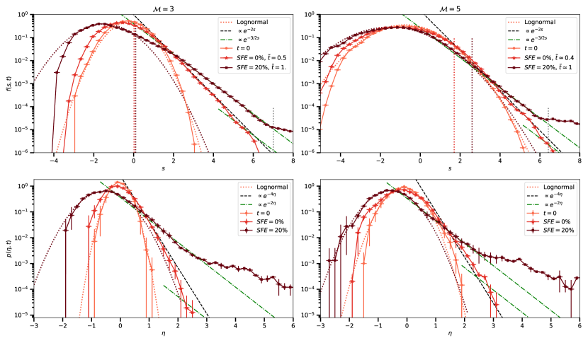
Figure 1: Evolution of the $s$ (top row) and $\eta$-PDFs (bottom row) for solenoidal simulations with $\mathcal{M}\simeq 3$, $N_{\rm res}=512$ (left) and $\mathcal{M}=5$, $N_{\rm res}=256$ (right) at $t=0$ (orange circles), SFE$=0\%$ (red stars) and SFE$=20\%$ (dark red squares). Horizontal error-bars represent bin spacing and vertical error-bars indicate the uncertainty in the $\eta$-PDFs corresponding to 3 different projection directions of the simulation box. Lognormal fits of the low density parts of PDFs at $t=0$ and SFE$=20\%$ are shown in dotted lines.The vertical dotted red lines corresponds to the value of $s_{\rm G}$ calculated from Eq. (35) with values of $(b\mathcal{M})$ and $\sigma_{s}$ calculated at time $\tilde{t}=t/\tau_{\rm ff,0}$. For $s>s_{\rm G}$ , the $s$-PDFs and $\eta$-PDFs first develop power-law tails with exponents $\alpha_{\eta}=2$, $\alpha_{\eta}=4$ (black dashed lines) and then $\alpha_{s}=3/2$, $\alpha_{\eta}=2$ (green dot-dashed lines) at higher density. The vertical dotted grey lines at $s>6$ correspond to $s_{\rm max}$ from Eq. (37).

After Eq. (25), we expect gravity to have a dominant contribution at densities $s>s_{\rm G}$, which yields here:

$$|\mathrm{e}^{s_{\rm G}}-1| \equiv (b\mathcal{M})^{2}\times\alpha_{\rm vir,0}\times\left|\frac{s_{\rm G}+\frac{1}{2}\sigma_{s}^{2}}{\sigma_{s}^{2}}\right|,$$ (35)

where $\alpha_{\rm vir,0}=5\sigma_{v}^{2}/(6GL_{\rm b}^{2}\rho_{0})$ is the virial parameter suited for a box of size $L_{\rm b}$ and 3D-velocity dispersion $\sigma_{v}$, as in Federrath & Klessen (2012, 2013). On the other hand, the maximum density $\rho_{\rm max}$ above which the simulations do not properly resolve the collapse and describe the statistics of the cloud reads (Truelove et al., 1997):

$$\rho_{\rm max}=\rho_{0}\,\mathrm{e}^{s_{\rm max}}=\frac{\pi c_{\rm s}^{2}}{16G\Delta x_{\rm min}^{2}},$$ (36)

with $\Delta x_{\rm min}$ the size of the most resolved cell. This condition can be rewritten

$$s_{\rm max}=\mathrm{ln}\left(\alpha_{\rm vir,0}\right)+2\,\mathrm{ln}\left(\frac{N_{res}}{\mathcal{M}}\right)+\mathrm{ln}\left(\frac{6\pi}{80}\right).$$ (37)

For $s>s_{\rm max}$, the lack of resolution will yield the development of shallow power-laws corresponding to the spurious fragmentation of these regions (see Fig. (1) below and Federrath & Klessen (2013)).

5.2 Evolution of the PDFs

Figure 2: $\eta_{\rm th}$, calculated from Eq. (34) and the $s$-PDF, vs. $\eta_{\rm mes}$, directly measured on the $\eta$-PDFs, for runs with $\mathcal{M}=3$, $5$, $10$ (light to dark red). Runs with $\mathcal{M}\sim 3$ and $\mathcal{M}=10$ have two values of $\eta_{\rm max}$, for each resolution $N_{\rm res}=256$ and $N_{\rm res}=512$. We note the excellent agreement between $\eta_{\rm mes}$ and $\eta_{\rm th}$.

Figure (1) compares our analytical calculations of the $s$ and $\eta$-PDFs with the solenoidal simulations for $\mathcal{M}\simeq 3$, $N_{\rm res}=512$ and $\mathcal{M}=5$, $N_{\rm res}=256$ at initial time $t=0$ (orange), and at star formation efficiencies SFE$=$0% (red) and SFE$=$20% (dark red). A major result of § 2.4 (Eqns. (25) and (35)) is the determination of a density threshold, $s_{\rm G}$ (resp. $\eta_{\rm G}$), above which the $s$-PDF (resp. $\eta$-PDF) is expected to develop power-law tails. Similarly, spurious shallow power-laws will develop above $s_{\rm max}$ (resp. $\eta_{\rm max}$). In both cases $\eta_{\rm G}$ and $\eta_{\rm max}$ can be obtained from the determination of the corresponding values on the $s$-PDF with Eq. (34). We note the excellent agreement between the theoretical and numerical curves over the whole range of densities. Notably, the theoretical determinations of $s_{\rm G}$ from Eq. (35), threshold of the gravity impacted domain, agree very well with the onset of a power law in the simulations. It is worth stressing that for the $\mathcal{M}\sim 3$ simulation, $s_{\rm G}\sim 0.1$ and $\alpha_{\rm vir}\ll 1$, and thus we do not expect the power law tail with exponent $\alpha_{s}=3/2$ to develop up to $s_{\rm G}$ in a time $\tilde{t}\simeq 1$ (since this requires typically a few $\tau_{\rm ff,0}$). However departures from a lognormal behavior are indeed seen to start at about $s\sim 0.1$.

Fig. (2) compares $\eta_{\rm mes}\equiv\eta_{\rm G_{\rm mes}},\,\eta_{\rm max_{\rm mes}}$, directly measured on various simulations, to $\eta_{\rm th}\equiv\eta_{\rm G_{\rm th}},\,\eta_{\rm max_{\rm th}}$ derived from Eq. (34) and the value of $s_{\rm G}$ and $s_{\rm max}$. As seen in the figure, the agreement between the theoretical value $\eta_{\rm th}$ and the measured one $\eta_{\rm mes}$ is remarkable.

6 Comparison with Observations

In this section, we confront our theory to observations of column density PDFs in various MCs. We use a simple model with one or two power-law tails, characterized by 1 or 2 transition densities, $s_{1}$ and $s_{2}$, between lognormal and power laws, as described in App. (E). From the determination of the variance $\sigma_{\rm s,\eta}$ in the lognormal parts of the PDF, we get an estimate of the product $(b\mathcal{M})$ (Eq. (23)), while from the determinations of $s_{1}$ and $s_{2}$ we get an estimate of $\alpha_{\rm vir}=5\sigma_{v}^{2}/(\pi GL_{\rm c}^{2}\overline{\rho})$, and of the time since the first regions started to collapse, in unit of mean free-fall time $\tilde{t}_{\rm coll}={t}_{\rm coll}/\tau_{\rm ff,0}$ (Eqs. (25), (32), (29)). The values are given in Table (1).

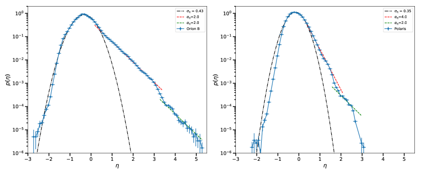
Figure 3: Left: Observed $\eta$-PDF of the cloud Orion B. Dash-dotted black line: lognormal fit of the low $\eta$ part of the PDF. Dashed red and green lines: power-law with exponent $\alpha_{\eta}=2$, corresponding to an underlying $s$-PDF with a power-law exponent $\alpha_{s}=3/2$, signature of collapsed regions. Right: Observed $\eta$-PDF of the cloud Polaris. Dash-dotted black line: lognormal fit of the low $\eta$ part of the PDF. Dashed red and green lines: power-laws respectively with exponents $\alpha_{\eta}=4$ and 2, corresponding to an underlying $s$-PDF transiting from a lognormal to power laws with exponents $\alpha_{s}=2$ and 3/2, respectively.

We apply our method to two different clouds: Orion B (Schneider et al., 2013; Orkisz et al., 2017) and Polaris (André et al., 2010; Miville-Deschênes et al., 2010; Schneider et al., 2013). The data were kindly provided by Nicola Schneider. For Orion B, the average column density is $\overline{N(H_{2})}=2.06\times 10^{21}\mathrm{cm}^{-2}$ and the cloud’s total mass and area above an extinction $A_{v}\geq 1$ are $M_{c,A_{v}\geq 1}=29.69\times 10^{3}M_{\odot}$ and $A_{c,A_{v}\geq 1}=651$ pc². For Polaris this yields $(\overline{N(H_{2})},M_{c,A_{v}\geq 1},A_{c,A_{v}\geq 1})=(1.73\,10^{21}\mathrm{cm}^{-2},1.21\times 10^{3}M_{\odot},3.9\,\mathrm{pc}^{2})$.

The first one, Orion B, contains numerous pre-stellar cores. Its $\eta$-PDF displays a lognormal part at low column densities and a power-law tail at high densities with exponent $\alpha_{\eta}\simeq 2$, corresponding to an underlying $s$-PDF with exponent $\alpha_{s}=3/2$, signature of collapsed regions, as seen in Fig. (3) (left). The power-law tail develops for $s>s_{1}=1.73^{+0.25}_{-0.23}$. We can thus estimate that in this cloud, (statistically significant, see §3) collapse of the densest regions has occured since $\tilde{t}_{\rm coll}\approx(2-5)\times\mathrm{e}^{-s_{1}/2}\gtrsim 1$ (see §3.3). Note here that $\tau_{\rm ff,0}$ corresponds to the region under study in the cloud, not to the global cloud itself. Estimation of $(b\mathcal{M})$ from the determination of $\sigma_{s}$ combined with estimation of $s_{1}$ yield $\alpha_{\rm vir}\sim 1$. The estimated $(b\mathcal{M})$ is compatible with mean Mach-numbers $\mathcal{M}=5.4^{+0.8}_{-0.8}$ for $b=1/3$ and $\mathcal{M}=3.6^{+0.5}_{-0.5}$ for $b=1/2$, in agreement with Orkisz et al. (2017).

Table 1: Properties of the clouds

Name	Func. form	$\sigma_{s}$	$(b\mathcal{M})$	$\mu$	$\alpha_{1}$	$\alpha_{2}$	$s_{1}$	$s_{2}$	$\alpha_{\rm vir}$	$\tilde{t}_{\rm coll}$
(1)	(2)	(3)	(4)	(5)	(6)	(7)	(8)	(9)	(10)	(11)
Orion B	Ln+1Pl	$1.2^{+0.09}_{-0.1}$	$1.8^{+0.26}_{-0.26}$	$-0.92^{+0.13}_{-0.11}$	$2$	$-$	$1.73^{+0.25}_{-0.23}$	$-$	$0.88^{+0.26}_{-0.23}$	$\gtrsim 1$
Polaris	Ln+2Pl	$0.98^{+0.07}_{-0.08}$	$1.27^{+0.16}_{-0.15}$	$-0.55^{+0.08}_{-0.07}$	$4$	$2$	$1.68^{+0.38}_{-0.34}$	$6.3^{+0.1}_{-0.15}$	$\lesssim 1.2$	$0.2\pm 0.1$

The second cloud, Polaris, where detectable star formation does not seem to have occurred yet, exhibits an extended power-law tail with a steep exponent, $\alpha_{\eta}\simeq 4$, corresponding to a $s$-PDF power-law tail of exponent $\alpha_{s}=2$ for $s>s_{1}$, before reaching the asymptotic values $\alpha_{\eta}\simeq 2$, i.e. $\alpha_{s}=3/2$ at high density, $s>s_{2}$, as seen in Fig. (3) (right). Carrying out the same analysis as for Orion B, we get $(s_{1},s_{2})=(1.68^{+0.38}_{-0.34},6.3^{+0.1}_{-0.15})$. The value of $s_{1}$ yields here $\tilde{t}_{\rm coll}\approx 0.5\,\mathrm{e}^{-s_{1}/2}=0.22^{+0.03}_{-0.04}$ for this cloud. The determination of the density $s_{2}$, which corresponds to collapsing regions, yields $\tilde{t}_{\rm coll}\approx$(2-5)$\times\mathrm{e}^{-s_{2}/2}\approx 0.09-0.21$, consistent with the above estimate of $\tilde{t}_{\rm coll}$, which we finally estimate as $\tilde{t}_{\rm coll}=0.2\pm 0.1$. The theory thus suggests that gravity has started dominating dense regions, corresponding to the onset of the first power law at $s=s_{1}$ only recently, i.e. for a short time $\tilde{t}_{\rm coll}$. According to these determinations, the quiescent Polaris region is quite young and has not even reached half its mean free-fall time yet. Eventually, we expect it to start forming detectable pre-stellar cores in a timescale of the order of its mean-free fall time, most likely in the “Saxophone” region, which entails most of the power-law part of its PDF (Schneider et al., 2013). Taking $s_{1}=s_{\rm G}$ yields an upper limit $\alpha_{\rm vir}\lesssim 1.2$. The estimated $(b\mathcal{M})$ for Polaris yields mean Mach numbers $\mathcal{M}=3.8^{+0.4}_{-0.4}$ and $\mathcal{M}=2.5^{+0.3}_{-0.3}$ for $b=1/3$ and $b=1/2$, respectively, consistent with the estimation of Schneider et al. (2013).

7 Conclusion

In this Letter, we have derived an analytical theory of the PDF of density fluctuations in supersonic turbulence in the presence of a gravity field in star-forming molecular clouds. The theory is based on a derivation of a combination of the coupled Navier-Stokes equations for the fluid motions and the Poisson equation for the gravity. The theory extends upon previous approaches (Pope, 1981, 1985; Pan et al., 2018, 2019b, 2019a) first by including gravity, second by considering the PDF as a dynamical system, not a stationary one. We derive rigorously the transport equations of the PDF, characterize its evolution and determine the density threshold above which gravity strongly affects and eventually dominates the dynamics of the turbulence. The theoretical results and diagnostics reproduce very well numerical simulations of gravoturbulent collapsing clouds (§5) and various available observations (§6).

A major result of the theory is the characterization of two density regions in the PDF (see §2.4). A low density region where gravity does not affect significantly the dynamics of turbulence so the PDF is the one of pure gravitationless turbulence, which resembles a lognormal form for isothermal, dominantly solenoidal turbulence. Then, above a density threshold, $s_{\rm G}$, given by Eqs. (25) and (35), gravity starts affecting significantly the turbulence, essentially by increasing the velocity dispersion (thus the variance). Above this threshold, $s>s_{\rm G}$, power-law tails develop over time in the $s$-PDF, $f(s,t)\propto e^{-\alpha_{s}s}$, i.e. $p(\eta,t)\propto e^{-\alpha_{\eta}\eta}$ for the $\eta$-PDF of the surface density, as a direct consequence of the rising impact of gravity upon turbulence (see §3). Within a typical timescale $\sim$$\tau_{\rm G}(s)=\tau_{\rm G,0}\,\mathrm{e}^{-s/2}$, with $\tau_{\rm G,0}\equiv 1/\sqrt{4\pi G\overline{\rho}}$, this yields the onset of a first power law tail with $\alpha_{s}\geq 2$, i.e. $\alpha_{\eta}\geq 4$. Later on, after a few $\tau_{\rm ff}(s)$ for a given density $s$, and/or at higher density, i.e. smaller scales, a second power law develops, with $\alpha_{s}=3/2$, i.e. $\alpha_{\eta}=2$. This is the signature of regions in free-fall collapse.

Another important result of this study is to provide a procedure to relate the observed thresholds in column density, corresponding to the onset of the two power-law tails in the $\eta$-PDF, to the corresponding ones in volume density in the $s$-PDF (see §4 and App. A). Combined with the results of §2.4 and §3, this allows to infer, from the observation of column-densities, various physical parameters characterizing molecular clouds (or regions of), notably the virial parameter $\alpha_{\rm vir}$. Moreover, the theory offers the possibility to date the clouds in units of $\tilde{t}_{\rm coll}$, i.e. the time since a statistically significant fraction of dense regions of the cloud started to collapse, normalized to the cloud’s mean free-fall time. This explains why clouds exhibiting $\eta$-PDF with steep power laws ($\alpha_{\eta}\geq 3$) or extended lognormal parts are quiescent, since they have a short “age” $\tilde{t}_{\rm coll}$. This applies to Polaris (André et al., 2010; Miville-Deschênes et al., 2010; Schneider et al., 2013) (§6) but could also explain the quiescence of Chamaelon III (De Oliveira et al., 2014).

The theory derived in this study allows the determination of the aforementioned volume and column density thresholds, $s_{G},\eta_{G}$, and the characteristic timescales $\tau_{\rm G}(s),\tilde{t}_{\rm coll}$ (Eqns (25),(32),(29),(34),(35)). This yields quantitative, predictive diagnostics, from either simulations or observations, to determine precisely the relative impact of gravity upon turbulence within star forming clouds/clumps and their evolutionary status. The theory thus provides a precise scale and clock to numericists and observers exploring star formation in MCs. It provides a sound theoretical foundation and quantitative diagnostics to analyze observations or numerical simulations of star-forming regions and to characterize the evolution of the density PDF in various regions of MCs. This theoretical framework provides a new vision on how gravitational collapse initiates and evolves within turbulent dense star-forming regions.

Appendix A Derivation of the expression of the source terms Eqs 14-16

To obtain the source terms Eqs. (14-16) that appear in Eq. (12), we start by taking the divergence of Eq. (2)

$$\partial_{t}\left(\bm{\nabla}\cdot\bm{v}\right)+\bm{\nabla}\cdot\left(\left\{\bm{v}\cdot\bm{\nabla}\right\}\bm{u}\right)+\bm{\nabla}\cdot\left(\left\{\bm{u}\cdot\bm{\nabla}\right\}\bm{V}\right)+\bm{\nabla}\cdot\left(\left\{\bm{V}\cdot\bm{\nabla}\right\}\bm{V}\right) = -4\pi\,G\,\rho-\bm{\nabla}\cdot\left(\frac{1}{\rho}\bm{\nabla}P\right).$$ (A1)

We then take the average of Eq. (A2) to obtain

$$\partial_{t}\left(\bm{\nabla}\cdot\bm{V}\right)+\bm{\nabla}\cdot\left(\left\{\bm{V}\cdot\bm{\nabla}\right\}\bm{V}\right) = -4\pi\,G\,\overline{\rho},$$ (A2)

where $\partial_{t}\left(\bm{\nabla}\cdot\bm{\overline{u}}\right)=\bm{\nabla}\cdot\left(\overline{\left\{\bm{v}\cdot\bm{\nabla}\right\}\bm{u}}\right)=\bm{\nabla}\cdot\left(\left\{\overline{\bm{u}}\cdot\bm{\nabla}\right\}\bm{V}\right)=\bm{\nabla}\cdot\left(\overline{\frac{1}{\rho}\bm{\nabla}P}\right)=0$, because the turbulent fields $\rho$ and $\bm{u}$ are statistically homogeneous and because of the barotropic E.O.S $P=P(\rho)$. Then, by subtraction, we obtain

$$\partial_{t}\left(\bm{\nabla}\cdot\bm{u}\right)+\bm{\nabla}\cdot\left(\left\{\bm{v}\cdot\bm{\nabla}\right\}\bm{u}\right)+\bm{\nabla}\cdot\left(\left\{\bm{u}\cdot\bm{\nabla}\right\}\bm{V}\right) = -4\pi\,G\,\overline{\rho}\left(\mathrm{e}^{s}-1\right)-\bm{\nabla}\cdot\left(\frac{1}{\rho}\bm{\nabla}P\right).$$ (A3)

We then note that $\bm{\nabla}\cdot\left(\left\{\bm{u}\cdot\bm{\nabla}\right\}\bm{V}\right)=\bm{u}\cdot\bm{\nabla}\left(\bm{\nabla}\cdot\bm{V}\right)+(\partial_{i}u_{j})(\partial_{j}V_{i})=(\partial_{i}u_{j})(\partial_{j}V_{i})=\bm{\nabla}\bm{V}:\bm{\nabla}\bm{u}$, because $\rho$ is homogeneous, and by expanding $\bm{\nabla}\cdot\left(\left\{\bm{v}\cdot\bm{\nabla}\right\}\bm{u}\right)$ we finaly obtain

$$\frac{\mathrm{D}\bm{\nabla}\cdot\bm{u}}{\mathrm{D}t}=-\bm{\nabla}\bm{u}:\bm{\nabla}\bm{u}-2\bm{\nabla}\bm{V}:\bm{\nabla}\bm{u}-4\pi\,G\,\overline{\rho}\left(\mathrm{e}^{s}-1\right)-\bm{\nabla}\cdot\left(\frac{1}{\rho}\bm{\nabla}P\right),$$ (A4)

giving the expression of the source terms Eqs. (14-16).

Appendix B Reciprocal of Eqs 27-28.

In §3 we have shown that a conditional expectation $\left<\bm{\nabla}\cdot\bm{u}|s,t\right>=h(t)\times\mathrm{e}^{as}$, with $a>0$, would produce a $s$-PDF with a power law tail with exponent $\alpha_{s}=a+1$, i.e $f(s)\propto\mathrm{e}^{-(a+1)s}$ (Eqs. 27-28). We show here the reciprocal.

Let us assume that the $s$-PDF, $f$, is non-static and has a power-law tail with exponent $\alpha_{s}=a+1$ with $a>0$. More precisely, let us assume that

$$f(s,t)=A(s,t)\,\mathrm{e}^{-(a+1)s},$$ (B1)

with a function $A(s,t)$ such as $A(s,t)\approx B(t)$ for $s\geq s_{c}$, for some $s_{c}$, where $B(t)$ is a $\mathcal{C}^{1}$ function of the time variable only, with a bounded derivative. Re-writing Eq. 9 as

$$\left\{\frac{\partial}{\partial s}+\frac{\partial\mathrm{ln}A}{\partial s}-a\right\}\left<\bm{\nabla}\cdot\bm{u}|s,t\right>=\frac{\partial\mathrm{ln}A}{\partial t},$$ (B2)

one obtains

$$\left<\bm{\nabla}\cdot\bm{u}|s,t\right>=C(t)\times A(s,t)^{-1}\times\mathrm{e}^{a\,s}+A(s,t)^{-1}\,\mathrm{e}^{as}\int_{s_{i}}^{s}\,\mathrm{e}^{-as^{\prime}}\frac{\partial A}{\partial t}(s^{\prime},t)\,\mathrm{d}s^{\prime},$$ (B3)

with $C(t)$ a function of the time variable only and $s_{i}$ some fixed density. As $f$ is not stationary, $\left<\bm{\nabla}\cdot\bm{u}|s,t\right>$ is not zero everywhere but, at any time $t$, there exists $s_{0}(t)$ such as $\left<\bm{\nabla}\cdot\bm{u}|s_{0}(t),t\right>=0$ to ensure $\overline{\bm{\nabla}\cdot\bm{u}}=0$. Then we can fix the function $C(t)$ to write without any loss of generality:

$$\left<\bm{\nabla}\cdot\bm{u}|s,t\right>=A(s,t)^{-1}\,\mathrm{e}^{as}\int_{s_{0}(t)}^{s}\,\mathrm{e}^{-as^{\prime}}\frac{\partial A}{\partial t}(s^{\prime},t)\,\mathrm{d}s^{\prime}.$$ (B4)

Then, because $a>0$ and $\partial_{t}B(t)$ is bounded, the integral on the r.h.s of Eq. B4 is bounded and converges rapidly towards $\int_{s_{0}(t)}^{+\infty}\,\mathrm{e}^{-as^{\prime}}\partial_{t}A(s^{\prime},t)\,\mathrm{d}s^{\prime}=I(t)$. The asymptotic behavior of $\left<\bm{\nabla}\cdot\bm{u}|s,t\right>$ for large $s\geq s_{c}$ is thus

$$\left<\bm{\nabla}\cdot\bm{u}|s,t\right>\approx I(t)\times B(t)^{-1}\times\mathrm{e}^{a\,s}=h(t)\times\mathrm{e}^{a\,s}.$$ (B5)

This shows that to a non-stationary $s$-PDF with a power-law tail of exponent $\alpha_{s}=a+1$ corresponds a conditional expectation $\left<\bm{\nabla}\cdot\bm{u}|s,t\right>\approx h(t)\times\mathrm{e}^{as}$ for $s\gg 1$.

Appendix C Transitions to power-law tails

In §4 we derived a way to relate the volume density at which the $s$-PDF, $f(s)$, develop power-laws to the column density at which the $\eta$-PDF, $p(\eta)$, develops a similar behaviour. We call $s_{\rm crit}$ the critical value corresponding to the beginning of a power-law tail in the $s$-PDF (Eq. (34).

Assuming ergodicity, we relate the volume fraction of regions with densities exceeding $s_{\rm crit}$ to the probability of finding a density exceeding $s_{\rm crit}$:

$$\frac{V\left(s\geq s_{\rm crit}\right)}{V(\mathrm{cloud})}=\int_{s_{\rm crit}}^{\infty}f(s)\mathrm{d}s.$$ (C1)

We now want to evaluate the projected area of this volume onto the plane perpendicular to the line of sight $S(s\geq s_{\rm crit})$. Assuming statistical isotropy we get :

$$\frac{S(s\geq s_{\rm crit})}{S(\mathrm{cloud})}\simeq\left(\frac{V\left(s\geq s_{\rm crit}\right)}{V(\mathrm{cloud})}\right)^{2/3}.$$ (C2)

We then identify regions on the observed area of the cloud contributing to the power-law in the $\eta$-PDF to regions included in the projected area $S(s\geq s_{\rm crit})$. This yields for the critical surface density $\eta_{\rm crit}$ at which the $\eta$-PDF transits to a power-law:

$$\int_{\eta_{\rm crit}}^{\infty}p(\eta)\mathrm{d}\eta=\frac{S(s\geq s_{\rm crit})}{S(\mathrm{cloud})}\simeq\left(\int_{s_{\rm crit}}^{\infty}f(s)\mathrm{d}s\right)^{2/3},$$ (C3)

which is Eq. (34).

Appendix D Numerical models

In each simulation, gravity is switched on and sink particles are allowed to form after a state of fully developed turbulence has been reached, which determines the initial conditions at $t=t_{0}=0$ in the simulation. The associated transport equations for these simulations are:

$$\bm{V} = 0,$$ (D1)

$$\overline{\rho} = \rho_{0},$$ (D2)

$$s = \mathrm{ln}\left(\rho/\rho_{0}\right),$$ (D3)

$$\frac{\mathrm{D}\bm{\nabla}\cdot\bm{u}}{\mathrm{D}t} = -\bm{\nabla}\bm{u}:\bm{\nabla}\bm{u}-4\pi G\rho_{0}\left(\mathrm{e}^{s}-1\right)\Theta(t)$$ (D4)

$$-c_{\rm s}^{2}\,\bm{\nabla}^{2}s+\bm{\nabla}\cdot\bm{F}_{\rm stir},$$

$$\frac{\partial}{\partial t}\left[\left<\left(\bm{\nabla}\cdot\bm{u}\right)^{n}|s\right>f\right] = \left\{1+\frac{\partial}{\partial s}\right\}\left[\left<\left(\bm{\nabla}\cdot\bm{u}\right)^{n+1}|s\right>f\right]$$ (D5)

$$+f\left<\frac{\mathrm{D}\left(\bm{\nabla}\cdot\bm{u}\right)^{n}}{\mathrm{D}t}|s\right>,$$

where $\rho_{0}$ is constant, $c_{\rm s}=0.2$ km.$\mathrm{s}^{-1}$ is the sound speed, $\bm{\nabla}\cdot\bm{F}_{\rm stir}$ is the divergence of the turbulent forcing, which is $0$ for a solenoidal driving, and $\Theta(t)$ is the Heaviside step function ensuring that gravity is plugged in at $t=0$. In all models the Mach number $\mathcal{M}$ slightly increases with time because of collapsing regions. For most models, this only amounts to a few percents except for the $\mathcal{M}\simeq 3$ simulations which start at $\mathcal{M}\simeq 2$ and end up at $\mathcal{M}\simeq 3-4$ because the virial parameter $\alpha_{\rm vir,0}=5\sigma_{v}^{2}/(6GL_{\rm b}^{2}\rho_{0})$ is very small (see their Table 1). We note that the aforementioned definition of $\alpha_{\rm vir,0}$ taken from Federrath & Klessen (2012, 2013) differs by the one we have introduced in §2.4 by a factor $\pi/6\simeq 1/2$, if the cloud size $L_{\rm c}$ is taken to be the box size $L_{\rm b}$. As there is no unique way of translating the dimension of a cubic box into that of a spherical cloud and in order to simplify the comparison between the simulations and our calculations, we keep their notation and definition.

Finally, to be consistent with the authors we describe the time evolution of the simulations by means of the reduced time $\tilde{t}=t/\tau_{\rm ff,0}$, which is the time in unit of mean free fall time $\tau_{\rm ff,0}\equiv\sqrt{\frac{3\pi}{32G\rho_{0}}}$, and by means of the star formation efficiency (SFE), which is set at $0\%$ at the formation of the first sink particle. The authors only extracted the PDFs up to SFE$=20\%$ which we will thus refer to as the “long time” of the runs.

Appendix E Model with one or two power-law tails.

In this section, we develop a simple model that allows to infer the global $s$-PDF of molecular clouds from the observations of $\eta$-PDFs. We assume that the PDFs are simply continuous and have only one power-law at high densities and a lognormal cutoff at low densities:

$$f(s) = A_{1}\,\mathrm{e}^{-\frac{(s-\mu)^{2}}{2\sigma_{s}^{2}}},\,\,s\leq s_{\rm crit}$$ (E1)

$$= A_{2}\,\mathrm{e}^{-\alpha_{s}\left(s-s_{\rm crit}\right)},\,\,s\geq s_{\rm crit}.$$

Enforcing the continuity and normalisation of $f$ as well as the necessary condition $\overline{\mathrm{e}^{s}}=1$ (from our definition of $s$ in Eq. (6)) we obtain:

$$A_{1} = A_{2}\,\mathrm{e}^{\frac{(s_{\rm crit}-\mu)^{2}}{2\sigma_{s}^{2}}}$$ (E2)

$$1 = \frac{1}{2}\,A_{1}\sqrt{2\pi\sigma_{s}^{2}}\,\left[1+\mathrm{erf}\left(\frac{s_{\rm crit}-\mu}{\sqrt{2}\sigma_{s}}\right)\right]+\frac{A_{2}}{\alpha_{s}}$$ (E3)

$$1 = A_{1}\sqrt{\frac{\pi}{2}\sigma_{s}^{2}}\,\mathrm{e}^{\mu+\frac{\sigma_{s}^{2}}{2}}\left[1+\mathrm{erf}\left(\frac{s_{\rm crit}-\mu-\sigma_{s}^{2}}{\sqrt{2}\sigma_{s}}\right)\right]$$ (E4)

$$+\frac{A_{2}\,\mathrm{e}^{s_{\rm crit}}}{\alpha_{s}-1}.$$

We now assume that the variance $\sigma_{s}$ in the lognormal part and the exponent $\alpha_{s}$ of the power-law tail are inferred from the observations of the $\eta$-PDF following §4. More precisely, to obtain the variance $\sigma_{s}$, we use the formula of Burkhart & Lazarian (2012), $\sigma_{\eta}^{2}=A_{\eta s}\times\sigma_{s}^{2}$, where $A_{\eta s}$ may depend on the forcing parameter $b$. For simulations of compressible turbulence without gravity and with solenoidal driving ($b=1/3$) they found from their best fit $A_{\eta s}\simeq 0.11$, while observations of molecular clouds yield a value $A_{\eta s}\simeq 0.12-0.16$ for a forcing parameter $b=0.5$, corresponding to a mixture of solenoidal and compressive driving. From §4, $A_{2}/\alpha_{s}$, thus $A_{2}$ is obtained from the observations. We are now left with a system of 3 equations for 3 unknown quantities, namely $s_{\rm crit}$, $\mu$ and $A_{1}$. We note that, in this model, the parameter $\mu$, that determines the peak of the lognormal part, is shifted to lower densities to ensure $\overline{\mathrm{e}^{s}}=1$. Injecting Eq. (E2) into Eq. (E3) yields a closed equation for the variable $x=\frac{s_{\rm crit}-\mu}{\sqrt{2}\sigma_{s}}$:

$$1=A_{2}\,\mathrm{e}^{x^{2}}\sqrt{2\pi\sigma_{s}^{2}}\,\Phi(x)+\frac{A_{2}}{\alpha_{s}},$$ (E5)

with $\Phi(x)=\frac{1}{2}\left[1+\mathrm{erf}(x)\right]$ the cumulative distribution function for the normal distribution. Eq. (E4) is then used to obtain $\mu$ and then $s_{\rm crit}$.

In case where the $\eta$-PDF exhibits two power-law tails with exponent $\alpha_{\eta}=4$ and $\alpha_{\eta}=2$ we simply assume the following functional form:

$$f(s) = A_{1}\,\mathrm{e}^{-\frac{(s-\mu)^{2}}{2\sigma_{s}^{2}}},\,\,s\leq s_{1}$$ (E6)

$$= A_{2}\,\mathrm{e}^{-\alpha_{1}\left(s-s_{1}\right)},\,\,s_{1}\leq s\leq s_{2}$$

$$= A_{2}\,\mathrm{e}^{-\alpha_{1}\left(s_{2}-s_{1}\right)}\,\mathrm{e}^{-\alpha_{2}\left(s-s_{2}\right)},\,\,s_{2}\leq s,$$

with $\alpha_{1}=2$ and $\alpha_{2}=3/2$, and change the procedure as follows. First, we build the $s$-PDF as if there was only one power-law with exponent $\alpha_{\eta}=4$ in the $\eta$-PDF with the aforementioned procedure to obtain $A_{1}$, $A_{2}$, $\mu$ and $s_{1}$. We then use Eq. (34) to obtain $s_{2}$:

$$\frac{A_{2}\,\mathrm{e}^{-\alpha_{1}\left(s_{2}-s_{1}\right)}}{\alpha_{2}}=\left(\int_{\eta_{2}}^{\infty}p(\eta)\mathrm{d}\eta\right)^{3/2},$$ (E7)

where $\eta_{2}$ is the column density at the beginning of the second power-law with exponent $\alpha_{\eta}=2$. This modified procedure, while simple to implement, is sufficiently accurate as $s_{2}$ is large and thus regions with $s>s_{2}$ only represent a particularly small fraction of the total volume ($\lesssim 10^{-5}$).

We confront this procedure to observations in §6. Errors arising from the determination of $\eta_{\rm crit}$ and $\sigma_{s}$ from the observations yield an error $\Delta s_{\rm crit}=\pm 0.3$ on $s_{\rm crit}$, which is reasonable.

References

- André et al. (2010) André, P., Men’shchikov, A., Bontemps, S., et al. 2010, Astronomy & Astrophysics, 518, L102
- Ballesteros-Paredes et al. (2011) Ballesteros-Paredes, J., Vázquez-Semadeni, E., Gazol, A., et al. 2011, Monthly Notices of the Royal Astronomical Society, 416, 1436
- Brunt et al. (2010) Brunt, C. M., Federrath, C., & Price, D. J. 2010, Monthly Notices of the Royal Astronomical Society, 403, 1507
- Burkhart & Lazarian (2012) Burkhart, B., & Lazarian, A. 2012, The Astrophysical Journal, 755, L19, doi: 10.1088/2041-8205/755/1/l19
- Burkhart et al. (2016) Burkhart, B., Stalpes, K., & Collins, D. C. 2016, The Astrophysical Journal Letters, 834, L1
- Cho & Kim (2011) Cho, W., & Kim, J. 2011, Monthly Notices of the Royal Astronomical Society: Letters, 410, L8
- Collins et al. (2012) Collins, D. C., Kritsuk, A. G., Padoan, P., et al. 2012, The Astrophysical Journal, 750, 13
- De Oliveira et al. (2014) De Oliveira, C. A., Schneider, N., Merín, B., et al. 2014, Astronomy & Astrophysics, 568, A98
- Donkov & Stefanov (2018) Donkov, S., & Stefanov, I. Z. 2018, Monthly Notices of the Royal Astronomical Society, 474, 5588
- Federrath & Klessen (2012) Federrath, C., & Klessen, R. S. 2012, ApJ, 761, 156, doi: 10.1088/0004-637X/761/2/156
- Federrath & Klessen (2013) —. 2013, The Astrophysical Journal, 763, 51
- Federrath et al. (2008) Federrath, C., Klessen, R. S., & Schmidt, W. 2008, The Astrophysical Journal Letters, 688, L79
- Federrath et al. (2010) Federrath, C., Roman-Duval, J., Klessen, R., Schmidt, W., & Mac Low, M.-M. 2010, Astronomy & Astrophysics, 512, A81
- Frisch (1995) Frisch, U. 1995, Turbulence: the legacy of AN Kolmogorov (Cambridge university press)
- Girichidis et al. (2014) Girichidis, P., Konstandin, L., Whitworth, A. P., & Klessen, R. S. 2014, The Astrophysical Journal, 781, 91
- Guszejnov et al. (2018) Guszejnov, D., Hopkins, P. F., & Grudić, M. Y. 2018, Monthly Notices of the Royal Astronomical Society, 477, 5139, doi: 10.1093/mnras/sty920
- Kainulainen et al. (2009) Kainulainen, J., Beuther, H., Henning, T., & Plume, R. 2009, Astronomy & Astrophysics, 508, L35
- Kainulainen et al. (2006) Kainulainen, J., Lehtinen, K., & Harju, J. 2006, Astronomy & Astrophysics, 447, 597
- Klessen (2000) Klessen, R. S. 2000, The Astrophysical Journal, 535, 869
- Kritsuk et al. (2007) Kritsuk, A. G., Norman, M. L., Padoan, P., & Wagner, R. 2007, The Astrophysical Journal, 665, 416
- Kritsuk et al. (2010) Kritsuk, A. G., Norman, M. L., & Wagner, R. 2010, The Astrophysical Journal Letters, 727, L20
- Ledoux & Walraven (1958) Ledoux, P., & Walraven, T. 1958, in Astrophysics II: Stellar Structure/Astrophysik II: Sternaufbau (Springer), 353–604
- Lee et al. (2015) Lee, E. J., Chang, P., & Murray, N. 2015, The Astrophysical Journal, 800, 49
- Lemaster & Stone (2008) Lemaster, M. N., & Stone, J. M. 2008, The Astrophysical Journal Letters, 682, L97
- Miville-Deschênes et al. (2010) Miville-Deschênes, M.-A., Martin, P., Abergel, A., et al. 2010, Astronomy & Astrophysics, 518, L104
- Miville-Deschênes et al. (2017) Miville-Deschênes, M.-A., Salomé, Q., Martin, P., et al. 2017, Astronomy & Astrophysics, 599, A109
- Orkisz et al. (2017) Orkisz, J. H., Pety, J., Gerin, M., et al. 2017, Astronomy & Astrophysics, 599, A99
- Pan et al. (2018) Pan, L., Padoan, P., & Nordlund, Å. 2018, The Astrophysical Journal Letters, 866, L17
- Pan et al. (2019a) —. 2019a, The Astrophysical Journal, 881, 155
- Pan et al. (2019b) —. 2019b, The Astrophysical Journal, 876, 90
- Passot & Vázquez-Semadeni (1998) Passot, T., & Vázquez-Semadeni, E. 1998, Physical Review E, 58, 4501
- Pope (1981) Pope, S. 1981, The Physics of Fluids, 24, 588
- Pope & Ching (1993) Pope, S., & Ching, E. S. 1993, Physics of Fluids A: Fluid Dynamics, 5, 1529
- Pope (1985) Pope, S. B. 1985, Progress in energy and combustion science, 11, 119
- Schneider et al. (2013) Schneider, N., André, P., Könyves, V., et al. 2013, The Astrophysical Journal Letters, 766, L17
- Schneider et al. (2012) Schneider, N. e. a., Csengeri, T., Hennemann, M., et al. 2012, Astronomy & Astrophysics, 540, L11
- Truelove et al. (1997) Truelove, J. K., Klein, R. I., McKee, C. F., et al. 1997, The Astrophysical Journal Letters, 489, L179
- Vazquez-Semadeni (1994) Vazquez-Semadeni, E. 1994, The Astrophysical Journal, 423, 681
- Vazquez-Semadeni & Garcia (2001) Vazquez-Semadeni, E., & Garcia, N. 2001, The Astrophysical Journal, 557, 727, doi: 10.1086/321688