HOLISMOKES - IV. Efficient mass modeling of strong lenses through deep learning

Modeling the mass distributions of strong gravitational lenses is often necessary in order to use them as astrophysical and cosmological probes. With the large number of lens systems ($\gtrsim$$10^{5}$) expected from upcoming surveys, it is timely to explore efficient modeling approaches beyond traditional Markov chain Monte Carlo techniques that are time consuming. We train a convolutional neural network (CNN) on images of galaxy-scale lens systems to predict the five parameters of the singular isothermal ellipsoid (SIE) mass model (lens center $x$ and $y$, complex ellipticity $e_{x}$ and $e_{y}$, and Einstein radius $\theta_{\text{E}}$). To train the network we simulate images based on real observations from the Hyper Suprime-Cam Survey for the lens galaxies and from the Hubble Ultra Deep Field as lensed galaxies. We tested different network architectures and the effect of different data sets, such as using only double or quad systems defined based on the source center and using different input distributions of $\theta_{\text{E}}$. We find that the CNN performs well, and with the network trained on both doubles and quads with a uniform distribution of $\theta_{\text{E}}$ $>0.5\arcsec$ we obtain the following median values with $1\sigma$ scatter: $\Delta x=(0.00^{+0.30}_{-0.30})\arcsec$, $\Delta y=(0.00^{+0.30}_{-0.29})\arcsec$, $\Delta\theta_{\text{E}}=(0.07^{+0.29}_{-0.12})\arcsec$, $\Delta e_{x}=-0.01^{+0.08}_{-0.09}$, and $\Delta e_{y}=0.00^{+0.08}_{-0.09}$. The bias in $\theta_{\text{E}}$ is driven by systems with small $\theta_{\text{E}}$. Therefore, when we further predict the multiple lensed image positions and time-delays based on the network output, we apply the network to the sample limited to $\theta_{\text{E}}>0.8\arcsec$. In this case the offset between the predicted and input lensed image positions is $(0.00_{-0.29}^{+0.29})\arcsec$ and $(0.00_{-0.31}^{+0.32})\arcsec$ for the $x$ and $y$ coordinates, respectively. For the fractional difference between the predicted and true time-delay, we obtain $0.04_{-0.05}^{+0.27}$. Our CNN model is able to predict the SIE parameter values in fractions of a second on a single CPU, and with the output we can predict the image positions and time-delays in an automated way, such that we are able to process efficiently the huge amount of expected galaxy-scale lens detections in the near future.

1 Introduction

Strong gravitational lensing has become a very powerful tool for probing various properties of the Universe. For instance, galaxy-galaxy lensing can help to constrain the total mass of the lens and, assuming a mass-to-light ratio (M/L) for the baryonic matter, also its dark matter (DM) fraction. By combining lensing with other methods like measurements of the lens’ velocity dispersion (e.g., Barnabè et al., 2011, 2012; Yıldırım et al., 2020) or the galaxy rotation curves (e.g., Hashim et al., 2014; Strigari, 2013), the dark matter can be better disentangled from the baryonic component and a 3D (deprojected) model of the mass density profile can be obtained. Such profiles are very helpful for probing cosmological models (e.g., Davies et al., 2018; Eales et al., 2015; Krywult et al., 2017).

Another application of strong lensing is to probe high-redshift sources thanks to the lensing magnification (e.g., Dye et al., 2018; Lemon et al., 2018; McGreer et al., 2018; Rubin et al., 2018; Salmon et al., 2018; Shu et al., 2018). In recent years, huge efforts have been made in reconstructing the surface brightness distribution of lensed extended sources. Together with redshift and kinematic measurements, these observations contain information about the evolution of galaxies at higher reshifts. If the mass profile of the lens is well constrained, the original unlensed morphology can be reconstructed (e.g., Warren & Dye, 2003; Suyu et al., 2006; Nightingale et al., 2018; Rizzo et al., 2018; Chirivì et al., 2020).

Lensed supernovae (SNe) and lensed quasars are very powerful cosmological probes. By measuring the time-delays of a lensing system with an object that is variable in brightness, one can use it to constrain, for example, the Hubble constant $H_{0}$ (e.g., Refsdal, 1964; Chen et al., 2019; Rusu et al., 2020; Wong et al., 2020; Shajib et al., 2020). This helps to assess the $4.4\sigma$ tension between the cosmic microwave background (CMB) analysis that gives $H_{0}=(67.36\pm 0.54)\leavevmode\nobreak\ \text{km s}^{-1}\text{Mpc}^{-1}$ for flat $\Lambda$ cold dark matter ($\Lambda$CDM; Planck Collaboration et al., 2018) and the local distance ladder with $H_{0}=(74.03\pm 1.42)\leavevmode\nobreak\ \text{km s}^{-1}\text{Mpc}^{-1}$ (SH0ES project; Riess et al., 2019). To date, time-delay lensing cosmography has been mainly based on lensed quasars as the chance of a lensed supernova (SN) is substantially lower. There are currently two lensed SNe known: one core-collapse SN behind a strong lensing cluster MACS J1149.5+222.3 (SN Refsdal; Kelly et al., 2015) and one SN type Ia behind an isolated lens galaxy (iPTF16geu; Goobar et al., 2017). Thanks to the upcoming wide field surveys in the next decades, like the Rubin Observatory Legacy Survey of Space and Time (LSST, Ivezic et al., 2008), this will change. LSST is expected to detect hundreds of lensed SNe (e.g., Goldstein et al., 2019; Wojtak et al., 2019). Therefore, it is important to be prepared for such exciting transient events in a fully automated and fast way. In particular, a fast estimation of time-delay(s) is important for optimizing the observing–monitoring strategy for time-delay measurements.

In addition to time-delay measurements, observing lensed SNe type Ia can help to answer outstanding questions about their progenitor systems (Suyu et al., 2020). The basic scenario is the single degenerate case where a white dwarf (WD) is stable until it reaches the Chandrasekhar mass limit (Whelan & Iben, 1973; Nomoto, 1982) by accreting mass from a nearby star. Today there are also alternative scenarios considered where the WD explodes before reaching the Chandrasekhar mass, the so-called sub-Chandrasekhar detonations (Sim et al., 2010). Another possibility for a SN Ia is the double-degenerated scenario where the companion is another WD (e.g., Pakmor et al., 2010) and both are merging to exceed the Chandrasekhar mass limit. It is still unclear which of the main scenarios is correct to describe the SN Ia formation, or if both are. To shed light on this debate, one possibility is to observe the SN Ia spectroscopically at very early stages, which is normally difficult because SN detections are often close to peak luminosity, past the early phase. If this SN is lensed, we can use the position of the first appearing image, together with a mass model of the underlying lens galaxy, to predict the position and time when the next images will appear. Here it is very important to react quickly, particularly to compute the mass model of the underlying lens galaxy based on imaging, as the time-delays of galaxy-galaxy strong lensing are typically on the order of days to weeks.

Since these strong lens observations are very powerful, several large surveys including the Sloan Lens ACS (SLACS) survey (Bolton et al., 2006; Shu et al., 2017), the CFHTLS Strong Lensing Legacy Survey (SL2S; Cabanac et al., 2007; Sonnenfeld et al., 2015), the Sloan WFC Edge-on Late-type Lens Survey (SWELLS; Treu et al., 2011), the BOSS Emission-Line Lens Survey (BELLS; Brownstein et al., 2012; Shu et al., 2016; Cornachione et al., 2018), the Dark Energy Survey (DES; Dark Energy Survey Collaboration et al., 2005; Tanoglidis et al., 2020), the Survey of Gravitationally-lensed Objects in HSC Imaging (SuGOHI; Sonnenfeld et al., 2018a; Wong et al., 2018; Chan et al., 2020; Jaelani et al., 2020), and surveys in the Panoramic Survey Telescope and Rapid Response System (Pan-STARRS; e.g., Lemon et al., 2018; Cañameras et al., 2020) have been conducted to find lenses. So far we have detected several thousand lenses, but mainly from the lower redshift regime. However, based on newer upcoming surveys like the LSST, which will target around $20,000$ $\text{deg}^{2}$ of the southern hemisphere in six different filters $(u,g,r,i,z,y)$, together with the Euclid imaging survey from space operated by the European Space Agency (ESA; Laureijs et al., 2011), we expect billions of galaxy images containing on the order of one hundred thousand lenses (Collett, 2015).

To deal with this huge amount of images there are ongoing efforts to develop fast and automated algorithms to find lenses in the first place. These methods are based on different identification properties, for instance on geometrical quantification (Bom et al., 2017; Seidel & Bartelmann, 2007), spectroscopic analysis (Baron & Poznanski, 2017; Ostrovski et al., 2017), or color cuts (Gavazzi et al., 2014; Maturi et al., 2014). Moreover, convolutional neural networks (CNNs) have also been extensively used in gravitational lens detection (e.g., Jacobs et al., 2017; Petrillo et al., 2017; Schaefer et al., 2018; Lanusse et al., 2018; Metcalf et al., 2019; Cañameras et al., 2020; Huang et al., 2020) as they do not require any measurements of the lens properties. Once a CNN is trained, it can classify huge amounts of images in a very short time, and is thus very efficient. Nonetheless, CNNs have limitations (e.g., completeness or accurate grading) and the performance strongly depends on the training set design as it encodes an effective prior (in the case of supervised learning). In this regard unsupervised or active learning might be promising future avenues for finding lenses.

However, these methods are only for finding the lenses; a mass model is necessary for further studies. Mass models of gravitational lenses are often described by parameterized profiles, where the parameters are optimized, for instance via Markov chain Monte Carlo (MCMC) sampling (e.g., Jullo et al., 2007; Suyu & Halkola, 2010; Sciortino et al., 2020; Fowlie et al., 2020). These techniques are very time and resource consuming as modeling one lens can take weeks or months, and they are thus difficult to scale up for the upcoming amount of data. With the success of CNNs in image processing, Hezaveh et al. (2017) showed the use of CNNs in estimating the mass model parameters of a singular isothermal ellipsoid (SIE) profile, and investigated further error estimations (Perreault Levasseur et al., 2017), analysis of interferometric observations (Morningstar et al., 2018), and source surface brightness reconstruction with recurrent inference machines (RIMs; Morningstar et al., 2019). While they mainly consider single-band images and subtract the lens light before processing the image with the CNN, Pearson et al. (2019) presented a CNN to model the image without lens light subtraction. However, for all deep learning approaches one needs a data set that contains the images and the corresponding parameter values for training, validation, and testing the network. As there are not that many real lensed galaxies known, both groups use mock lenses for their CNNs.

We recently initiated the Highly Optimized Lensing Investigations of Supernovae, Microlensing Objects, and Kinematics of Ellipticals and Spirals (HOLISMOKES) program (Suyu et al., 2020, hereafter HOLISMOKES I). After presenting our lens search project (Cañameras et al., 2020, hereafter HOLISMOKES II), we present in this paper a CNN for modeling strong gravitationally lensed galaxies with ground-based imaging, taking advantage of four different filters and not applying lens light subtraction beforehand. In contrast to Pearson et al. (2019), we use a mocked-up data set based on real observed galaxy cutouts since the performance of the CNN on real systems will be optimal when the mock systems used for training are as close to real lens observations as possible. Our mock lens images contain, by construction, realistic line-of-sight objects as well as realistic lens and source light distributions in the image cutouts. We use the Hyper Suprime-Cam (HSC) Subaru Strategic Program (SSP) images together with redshift and velocity dispersion measurements from the Sloan Digital Sky Survey (SDSS) for the lens galaxies, and images together with redshifts from the Hubble Ultra Deep Field (HUDF) survey for the sources (Beckwith et al., 2006; Inami et al., 2017).

The outline of the paper is as follows. We describe in Sect. 2 how we simulate our training data, and we give a short introduction and overview of the used network architecture in Sect. 3. The main networks are presented in Sect. 4, and we give details of further tests in Sect. 5. We also consider the image position and time-delay differences in Sect. 6 for a performance test, and compare them to other modeling techniques in Sect. 7. We summarize and conclude our results in Sect. 8. Throughout this work we assume a flat $\Lambda$CDM cosmology with a Hubble constant $H_{0}=72\,\text{km}\,\text{s}^{-1}\,\text{Mpc}^{-1}$ (Bonvin et al., 2017) and $\Omega_{\text{M}}=1-\Omega_{\Lambda}=0.32$ (Planck Collaboration et al., 2018). Unless specified otherwise, each quoted parameter estimate is the median of its 1D marginalized posterior probability density function, and the quoted uncertainties show the 16th and 84th percentiles (i.e., the bounds of a 68% credible interval).

2 Simulation of strongly lensed images

For training a neural network one needs, depending on the network size, from tens of thousands to millions of images, together with the expected network output, which in our case are the values of the SIE profile parameters corresponding to each image. Since there are far too few known lens systems, we need to mock up lens images. While previous studies are based on partly or fully generated light distributions (e.g., Hezaveh et al., 2017; Perreault Levasseur et al., 2017; Pearson et al., 2019), we aim to produce more realistic lens images by using real observed images of galaxies and simulating only the lensing effect with our own routine. We work with the four HSC filters, $g,r,i$, and $z$ (respectively matched to HST filters F435W ($\overline{\lambda}=4343.4\AA$), F606W ($\overline{\lambda}=6000.8\AA$), F775W ($\overline{\lambda}=7702.2\AA$), and F850LP ($\overline{\lambda}=9194.4\AA$)) to give the network the color information to distinguish better between lens and source galaxies. The images of HSC for these filters are very similar to the expected image quality of LSST, such that our tests and findings will also hold for LSST. Therefore, this work is in direct preparation for and an important step in modeling the expected 100,000 lens systems that will be detected with LSST in the near future.

2.1 Lens galaxies from HSC

For the lenses we use HSC SSP images from the second public data release (PDR2; Aihara et al., 2019) with a pixel size of $0.168\arcsec$. To calculate the axis ratio $q_{\text{light}}$ and position angle $\theta_{\text{light}}$ of the lens, we use the second brightness moments calculated for the $i$ band since redder filters follow better the stellar mass; however, the S/N is substantially lower in the $z$ band compared to the $i$ band. We cross-match the HSC catalog with the SDSS catalog to use only images of galaxies where we have SDSS spectroscopic redshifts and velocity dispersions. With this selection we end up with a sample containing 145,170 galaxies that is dominated by luminous red galaxies (LRGs). We show in Figure 1 a histogram of the lens redshifts used for the simulation (in gray). We already overplot the distribution of the mock samples discussed in Sect. 4.

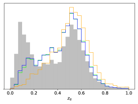
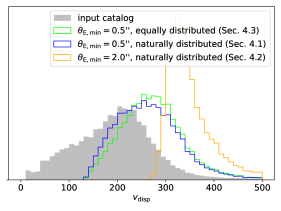
Figure 1: Distributions of the lens galaxy redshifts $z_{\text{d}}$ (top) and velocity dispersion $v_{\text{disp}}$ (bottom). Shown are the distributions of the input catalogs to the simulation code (in gray), and the distributions of the generated samples discussed in Sect. 4 (see inset for color-coding).

To describe the mass distribution of the lens, we adopt a SIE profile (Barkana, 1998) such that the convergence (dimensionless surface mass density) can be expressed as

$$\kappa(x,y)=\frac{\theta_{\text{E}}}{(1+q)r}$$ (1)

with elliptical radius

$$r=\sqrt{x^{2}+\frac{y^{2}}{q^{2}}},$$ (2)

where $x$ and $y$ are angular coordinates on the lens plane with respect to the lens center. In this equation $\theta_{\text{E}}$ denotes the Einstein radius and $q$ the axis ratio. The mass distribution is rotated by the position angle $\theta$. The Einstein radius is obtained from the velocity dispersion $v_{\text{disp}}$ with

$$\theta_{\text{E}}=4\pi\frac{v_{\text{disp}}^{2}}{c^{2}}\frac{D_{\text{ds}}}{D_{\text{s}}},$$ (3)

where $c$ is the speed of light, and $D_{\text{ds}}$ and $D_{\text{s}}$ are respectively the angular diameter distances between the lens (deflector) and source and the observer and source. The distribution of the velocity dispersion is shown in Figure 1 (bottom pannel, gray histogram). We compute the deflection angles of the SIE with the lensing software Glee (Suyu & Halkola, 2010; Suyu et al., 2012).

Based on the second brightness moments of the lens light distribution in the $i$ band, the axis ratio $q_{\text{light}}$ and position angle $\theta_{\text{light}}$ are obtained internally in our simulation code. Based on several studies (e.g, Sonnenfeld et al., 2018b; Loubser et al., 2020), the light traces the mass relatively well but not perfectly. Therefore, we add randomly drawn Gaussian perturbations on the light parameters, with a Gaussian width of $0.05\arcsec$ for the lens center, $0.05$ for the axis ratio, and $0.17$ radians (10 degrees) for the position angle, and adopt the resulting parameter values for the lens mass distribution. If the axis ratio of the mass $q$ (i.e., with Gaussian perturbation) is above 1, we draw a second realization of the Gaussian noise. If the resulting $q$ (from the second Gaussian perturbation) is $\leq 1$, then we keep this value; otherwise, we set $q$ to exactly 1.

While the simulation code assumes a parameterization in terms of axis ratio $q$ and position angle $\theta$, we parameterize for our network in terms of complex ellipticity $e_{\text{c}}$, which we define as $e_{\text{c}}=A\leavevmode\nobreak\ e^{2i\theta}=e_{x}+ie_{y}$ with

$$e_{x} = \frac{1-q^{2}}{1+q^{2}}\,\cos(2\theta),$$

$$e_{y} = \frac{1-q^{2}}{1+q^{2}}\,\sin(2\theta).$$ (4)

The back transformation is given by

$$\begin{array}[]{ll}q=&\sqrt{\frac{1-\sqrt{e_{x}^{2}+e_{y}^{2}}}{1+\sqrt{e_{x}^{2}+e_{y}^{2}}}}\\ \theta=&\left\{\begin{array}[]{ll}\frac{1}{2}\arccos\left(e_{y}\,\frac{1+q^{2}}{1-q^{2}}\right)&\text{ if }e_{x}>0\\ \frac{\pi}{2}+\left|\frac{1}{2}\arcsin\left(e_{x}\,\frac{1+q^{2}}{1-q^{2}}\right)\right|&\text{ if }e_{x}<0\end{array}.\right.\end{array}$$ (5)

This is in agreement with previous CNN applications to lens modeling (Hezaveh et al., 2017; Pearson et al., 2019).

2.2 Sources from HUDF

The images for the sources are taken from HUDF where the spectroscopic redshifts are also known (Beckwith et al., 2006; Inami et al., 2017). The cutouts are approximately $10\arcsec\times 10\arcsec$ with a pixel size of $0.03\arcsec$. This survey is chosen for its high spatial resolution, and we can adopt the images without point spread function (PSF) deconvolution. Moreover, it contains high-redshift galaxies such that we can achieve a realistic lensing effect. The 1,323 relevant galaxies are extracted with Source Extractor (Bertin & Arnouts, 1996) since the lensing effect is redshift dependent and we would otherwise lens the neighboring objects as if they were all at the same redshift, which would lead to incorrect lensing features. We show a histogram of the source redshifts in Figure 2 (gray histogram). Since we randomly select a background source (see Sect. 2.3 for details), the source galaxies can be used multiple times for one mock sample, and thus the redshift distribution varies slightly between the different samples (colored histograms; see details in Sect. 4).

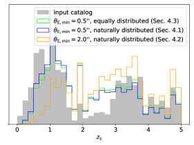
Figure 2: Distributions of the source redshifts $z_{\text{s}}$ of the input catalog to the simulation code (gray) and of the different mock samples (colors) discussed in Sect. 4.

2.3 Mock lens systems

To train our networks we use mock images based on real observed galaxies, and only generate the lensing effect. We use HSC galaxies as lenses (see Sect. 2.1 for details) and HUDF galaxies as background objects (see Sect. 2.2) to obtain mocks that are as realistic as possible. Figure 3 shows a diagram of the simulation pipeline. The input has three images: the lens, the unlensed source, and the lens PSF image (top row). Together with the provided redshifts of source and lens, as well as the velocity dispersion for calculating the Einstein radius with equation 3, the source image can be lensed onto the lens plane (second row). For this we place a random source from our catalog randomly in a specified region behind the lens and accept this position if we obtain a strongly lensed image. Since the source images have previously been extracted, we use the brightest pixel in the $i$ band to center the source. We have also implemented the option to just keep one of the two strong lens configurations, either quadruply or doubly imaged galaxies, classified based on the image multiplicity of the lensed source center. We also set a peak brightness threshold for the arcs based on the background noise of the lens. To estimate the background noise we take the corner with size 10%$\times$10% square of the full lens image (rounded to an integer of pixel) with the lowest maximum and compute from the patch the root mean square (RMS) value used as background noise. We take the lowest maximum for each corner separately and then compute the RMS of that one because there might be line-of-sight objects in the corners that would raise the RMS values. To avoid contamination to the background estimation from the lens, we use $40\arcsec\times 40\arcsec$ image cutouts such that each corner is $4\arcsec\times 4\arcsec$. The peak brightness of the lensed source must then be higher than the RMS to be accepted by the simulation code.

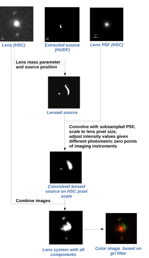
Figure 3: Diagram of the simulation pipeline.

In the next step the lensed source image with high resolution is convolved with the subsampled PSF of the lens, which is provided by HSC SSP PDR2 for each image separately. After binning the high-resolution lensed, convolved source image to the HSC pixel size and accounting for the different photometric zeropoints of the source telescope $\text{zp}_{\text{sr}}$ and lens telescope $\text{zp}_{\text{ls}}$, which gives a factor of $10^{0.4(\text{zp}_{\text{ls}}-\text{zp}_{\text{sr}})}$, the lensed source image is obtained as if it had been observed through the HSC instrument (third row in Figure 3), i.e., on the HSC 0.168″/pixel resolution. At this point we neglect the additional Poisson noise for the lensed arcs. Finally, the original lens and the mock lensed source images can be combined, which results in the final image (fourth row) that is cropped to a size of $64\times 64$ pixels ($10.8\arcsec\times 10.8\arcsec$). For better illustration, a color image based on the filters $g$, $r$, and $i$ is also shown, but we generate all mock images in four bands, which we use for the network training. We show more example images based on $gri$ filters in Figure 4. During this simulation, we set an upper limit on the Einstein radius of $5\arcsec$, which corresponds to the size of the biggest Einstein radius so far observed from galaxy-galaxy lensing (Belokurov et al., 2007).

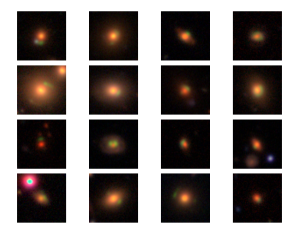
Figure 4: Examples of strong gravitational lens systems mocked up with our simulation code by using HUDF galaxies as sources behind HSC galaxies as lenses. Each image cutout is $10.8\arcsec\times 10.8\arcsec$.

We test the effect of different assumptions on the data set, like splitting up in quads-only or doubles-only, or different assumptions on the distribution of the Einstein radii since we found this to be crucial for the network performance. For this we generate with this pipeline new independent mock images that are based on the same lens and source images, but different combinations and alignments. The details of the different samples and the network trained on them will be discussed further in Sect. 4. For the set of quads-only and higher limit on the Einstein radius of 2″ we use a modification of the conventional data augmentation in deep learning. In particular, we rotate only the lens image before adding the random lensed source image, but not the whole final image (which is done normally for data augmentation). Thus, the ground truth values are also not exactly the same values given the change in position angle and another background source with different location and redshift.

3 Neural networks and their architecture

Neural networks (NNs) are extremely powerful tools for a wide range of tasks, and thus in recent years broadly used and explored. Additionally, the computational time can be reduced notably compared to other methods. There are generally two types of NNs: (1) classification, where the ground truth uses different labels to distinguish between the different classes, and (2) regression, where the ground truth consists of a set of parameters with specific values. The latter is the kind we use here, which means that the network predicts a numerical value for each of the five different SIE parameters ($x$, $y$, $e_{x}$, $e_{y}$, and $\theta_{\rm E}$).

Depending on the problem the network needs to solve, there are several different types of networks. Since we are using images as data input, typically convolutional layers followed by fully connected (FC) layers are used (e.g., Hezaveh et al., 2017; Perreault Levasseur et al., 2017; Pearson et al., 2019). The detailed architecture depends on attributes such as the specific task, the size of the images, or the size of the data set. We have tested different architectures and found an overall good network performance with two convolutional layers followed by three FC layers, but no significant improvement for the other network architectures. A sketch of this is shown in Figure 5. The input has four different filter images for each lens system and each image a size of $64\times 64\leavevmode\nobreak\ \text{pixels}$. The convolutional layers have a stride of 1 and a kernel size of $5\times 5\times C$, with $C=4$ for the first layer and $C=6$ for the second layer. Each convolutional layer is followed by a max-pooling layer of size $f\times f=2\times 2$ and stride 2. We use as activation function the rectified linear activation (ReLu) function. After the two convolutional layers, we obtain a data cube of size $13\times 13\times 16$, which is then passed through the FC layers after flattening to finally obtain the five output values. This network is coded with python 3.8.0 and uses pytorch modules (torch 1.5.1).

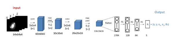
Figure 5: Overview of our main CNN architecture. The input has four different filter images for each lens system and each image a size of $64\times 64$ pixels. The network contains two convolutional layers (conv) each followed by a max-pooling layer (max pool) with kernel size $f$ and stride $S$ values indicated in the figure. This is then followed, after flattening the data cube, by three fully connected (FC) layers to finally obtain the five output values of the SIE $\eta$, containing the lens center $x$ and $y$, the complex ellipticity $e_{x}$ and $e_{y}$, and the Einstein radius $\theta_{\text{E}}$.

Independent of the exact network architecture, the network can contain hundreds of thousands of neurons or more. While initially the values of weight parameters and bias of each neuron are random, they are updated during the training. To see the network performance after the training, the data set is split into three samples: the training, the validation, and the test sets. We further divide those sets into random batches of size $N$. In each iteration the network predicts the output values for one batch (forward propagation), and after running over all batches from the training and validation sets, one epoch is finished. The error, which is called loss, is obtained for each batch with the loss function; we use the mean square error (MSE) defined as

$$L=\frac{1}{p\times N}\sum_{k=1}^{N}\sum_{l=1}^{p}(\eta^{\text{pred}}_{k,l}-\eta^{\text{tr}}_{k,l})^{2}\times w_{l}\,,$$ (6)

where $\eta_{k,l}^{\text{tr}}$ and $\eta_{k,l}^{\text{pred}}$ respectively denotes the $l{th}$ true and predicted parameter, in our case from $\{x,y,e_{x},e_{y},\theta_{\text{E}}\}$, of lens system $k$, and $p$ denotes the number of output parameters. We incorporated in our loss function $L$ weighting factors $w_{l}$, which are normalized such that $\sum_{l=1}^{p}w_{l}=p$ holds. This gives a weighting factor of 1 for all parameters if they are all weighted equally.

The loss value of that batch is then propagated to the weights and biases (back propagation) for an update based on a stochastic gradient descent algorithm to minimize the loss. This procedure is repeated in each epoch first for all batches of the training set and an average loss is obtained for the whole training set. Afterwards the steps are repeated for all batches of the validation set, while no update of the neurons is done, and an average loss for the validation set is obtained as well. The validation loss shows whether the network improved in that epoch or if a decreasing training loss is related to overfitting the neurons. A network is overfitting when it learns the training set, and not the features in the training set. After each epoch we reshuffle our whole training data to obtain a better generalization. This concludes one epoch, which is repeated iteratively to obtain a network with optimal accuracy.

This whole training corresponds to one so-called cross-validation run, where several cross-validation runs are performed by exchanging the validation set with another subset of the training set. For example, if the training set and validation set form five subsets {A, B, C, D, and E}, then we can have five independent runs of training where in each run the validation set is one of these five subsets and the training set contains the remaining four subsets. After the multiple runs, we can determine the optimal number of epochs for training by locating the epoch with the minimum average validation loss across the multiple runs. This procedure helps to minimize potential bias to certain types of lenses for a potentially unbalanced single split. The neural network trained on all five sets {A, B, C, D, E} up to that epoch is the final network, which is then applied to the test set that contains data the network has never seen before. In our case we used $\sim$56% of the data set as the training set, $\sim$14% as the validation set, and $\sim$30% as the test set in order to have a five-fold cross-validation for each network.

To find the best hyperparameter values for our specific problem, we test each network on its performance with several different variations of the hyperparameters. Independent of the data set, we train each cross validation run for 300 epochs, and apart from a few checks with different values, we fix the weight decay to 0.0005 and the momentum to 0.9. For the learning rate, batch size, and the initializations of the neurons, we perform a grid search, varying the learning rate $r_{\text{learn}}\in[0.1,0.05,0.01,0.008,0.005,0.001,0.0005,0.0001]$ and batch size as 32 or 64 images per batch, and exploring three different network initializations. For the weighting factors of the contribution to the loss we test two options, either all parameters contribute equally (i.e., $w_{l}=1\leavevmode\nobreak\ \forall\leavevmode\nobreak\ l$ in eq. 6) or the contribution of the Einstein radius is a factor of 5 higher ($w_{\theta_{\text{E}}}=5$). This already gives 96 different combinations of hyperparameters which we test with cross-validation and early stopping.

For a subset of the hyperparameter combinations, we test further possibilities. In particular, we explore the effect of drop-out (i.e., the omission of random neurons in every iteration) with a drop-out rate $p\in[0.1,0.3,0.5,0.7,0.9],$ but find no improvement. We further test different network architectures by adding an additional convolutional layer or fully connected layer, or by varying the number of neurons in the different layers. We also test a different weighting of the lens center parameters to the loss that is motivated by the results of our networks in Section 4.

In addition, we test the effect of five different scaling options of the input images for our data set, but assume here the learning rate $r_{\text{learn}}=0.001$ for simplicity. First, we boost the $r$ band by a factor of 10. Since the network is still able to recover the parameter values, we see that the network performance is not heavily affected by the absolute value of the images. Second, if we normalize each filter of one lens system independently of the other filters, the network fails to recover the correct parameter values. This shows us that the network is indeed able to extract the color information as the relative difference is much smaller, and thus needs the different filters. In the third and fourth option we normalize each filter with its maximum value or with the mean peak value of the different filters. Last, we also rescale the images by shifting them by the mean value and dividing by the standard deviation. Since we obtained no notable improvement with any one of these scalings, we use the images without rescaling to obtain our final networks.

4 Results

To train our modeling network we mock up lensing systems based on real observed galaxies with our simulation pipeline (see Sect. 2). Each lensing system is simulated in the four different filter $griz$ of HSC to give the network color information to distinguish better between lens galaxy and lensed arcs. The network architecture assumes, as described in Sect. 3 in detail, images 64 $\times$ 64 pixels in size, which corresponds to a size of around $10\arcsec\times 10\arcsec$.

During our network testing, we found that the distribution of Einstein radii in the training set is very important, especially as this is a key parameter of the model. Therefore, we trained a network under the assumption of different underlying data sets, for example a lower limit of the Einstein radius for the simulations or a different distribution of Einstein radii. We further tested the network performance by limiting to a specific configuration (i.e., only doubles or quads). We give an overview of the different data set assumptions in Table 1, as well as the best hyperparameter values that depend on the assumed data set.

Table 1: Overview of trained networks.

Natural distribution of Einstein radii of lenses
double	quad	$\theta_{\text{E,min}}$ [″]	$w_{\theta_{\text{E}}}$	loss	epoch	$r_{\text{learn}}$	$N$	seed	Section	Figures
✓	✓	0.5	1	0.0201	115	0.005	64	3	4.1
✓	✓	0.5	5	0.0496	123	0.001	64	3	4.1	6, 7, 8, 13, 14
✓	✓	2.0	1	0.0120	85	0.01	32	3	4.2
✓	✓	2.0	5	0.0209	85	0.008	32	2	4.2	7, 8, 9, 13, 14
✓		0.5	1	0.0193	242	0.008	64	1	5.1
✓		0.5	5	0.0474	117	0.001	64	3	5.1
✓		2.0	1	0.0118	163	0.05	64	3	5.1
✓		2.0	1	0.0118	96	0.01	32	2	5.1
✓		2.0	5	0.0217	62	0.008	32	3	5.1
	✓	0.5	1	0.0193	151	0.008	32	2	5.1
	✓	0.5	5	0.0441	69	0.001	32	2	5.1
	✓	2.0	1	0.0129	267	0.01	64	2	5.1
	✓	2.0	5	0.0268	285	0.005	32	1	5.1
Uniform distribution of Einstein radii of lenses
double	quad	$\theta_{\text{E,min}}$ [″]	$w_{\theta_{\text{E}}}$	loss	epoch	$r_{\text{learn}}$	$N$	seed	Section	Figures
✓	✓	0.5	1	0.0223	147	0.001	32	1	4.3
✓	✓	0.5	5	0.0528	112	0.0005	64	2	4.3	7, 8, 10, 11, 13, 14
	✓	0.5	1	0.0288	73	0.008	64	2	5.1
	✓	0.5	5	0.0688	56	0.001	32	2	5.1	12

Note. The first and second columns indicate if quads and/or doubles are included in the data set. The parameter $\theta_{\text{E,min}}$ represents the lower limit on the Einstein radius in the simulation, and $w_{\theta_{\text{E}}}$ is the weighting factor of the Einstein radius in the loss function. The other parameters (lens center, ellipticity) are always weighted by a factor of 1 and the sum of all five weighting factors is normalized to the number of parameters. The fifth and sixth columns give the value of the loss of the test set and the epoch with the best validation loss. This is followed by the specific hyperparameters: learning rate $r_{\text{learn}}$, batch size $N$, and seed for the random number generator. The last two columns list the sections and the figures that present the results of the corresponding network.

We present in the following subsections our CNN modeling results for various data sets.

4.1 Naturally distributed Einstein radii with lower limit $0.5\arcsec$

For this network we use 65,472 mock lens images simulated following the procedure described in Sect. 2. Here we assume a lower limit of the Einstein radii of $0.5\arcsec$ as otherwise the lensed source is totally blended with the lens and is not resolvable given the average seeing and image quality. The resulting redshift distributions are shown as the blue histograms for the lens in Figure 1 (top panel) and for the source in Figure 2. The lens redshift peaks at $z_{\text{d}}\sim 0.5$. Concerning the possible strong lensing configurations, the data set is dominated by doubles as expected. In addition, systems with smaller Einstein radii are more numerous than those with larger Einstein radii, as expected given the lens mass distribution, although the velocity dispersion (see Figure 1, bottom panel) peaks at around $v_{\text{disp}}\sim 280\,\text{km}\,\text{s}^{-1}$, and thus tends to include more massive galaxies than the input catalog (gray histogram). The distribution of the different parameters are shown in Figure 6, left panel; the red histogram depicts the true distribution and the blue one the predicted distribution. In the right panel we show the correlation between the true value and the predicted value for the five different parameters.

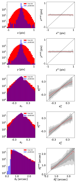
Figure 6: Network performance on the Einstein radius under the assumption of a lowest Einstein radius $\theta_{\text{E,min}}$ of 0.5″and a weighting factor of $w_{\theta_{\text{E}}}=5$. The left panel shows histograms of the ground truth (tr) in red and of the predicted values in blue. The right panel shows a direct comparison of the predicted against the true value, where the red line indicates the median of the distribution and the gray bands give the 1$\sigma$ (16th to 84th percentile) and 2$\sigma$ ( 2.5th to 97.5th percentile) ranges. From top to bottom are the five different model parameters, lens center $x$ and $y$, complex ellipticity $e_{x}$ and $e_{y}$, and Einstein radius $\theta_{\text{E}}$. For all plots 30 bins over the plotting range are used.

If we look at the performance on the lens center, which is measured in units of pixels with respect to the image cutout center, it seems as if the network fails totally in the first instance. We recall here how we obtain the lens mass center. In the simulation, we assume the lens light center to be the image center, and add a Gaussian variation (with standard deviation of $0.05\arcsec$) to shift to the lens mass center. Thus, the ground truth (red histogram in Figure 6) follows a Gaussian distribution, while the predicted lens center distribution (blue) is peakier. This suggests that the network does not obtain enough information from the slight shift or distortion in the lensed arcs to correctly predict the lens mass center. We test upweighting the contribution of the lens center to the loss with a higher fraction, which results in a better performance on these two parameters, but then the performance on the other parameter deteriorates. We thus refrain from upweighting the lens center. Further difficulties on the centroid parameters are caused by all systems having the exact same lens light center (which is at the center of the image). If we assume that the lens mass perfectly follows the light distribution and the lens light center is always the same, the lens (mass) center ground truth will become a delta distribution, and the network will perform much better.Accordingly, in many automated lens modeling architectures (e.g., Pearson et al., 2019) the lens center is not even predicted. Since the difference of the center for nearly all lens systems is smaller than $\pm 1$ pixel, it does not affect the model noticeably. We nonetheless keep five parameters for generality, and suggest investigating in future work more in this direction by relaxing the strict assumption of coincidence centers of image cutout and of lens light.

Looking at the performance on the ellipticity, it turns out that most of the lens systems are approximately round (i.e., $e_{x}\sim e_{y}\sim 0$) and that the network can recover them very well. If the lens is more elliptical, the network performance starts to drop. This might be an effect of the lower number of such lens systems in the sample especially since the position angle becomes relevant, and thus the number of systems in a particular direction is again lower. We note that $e_{x}=\pm 0.3$ and $e_{y}=0$ corresponds to an axis ratio $q=0.73$ (i.e., quite elliptical). If the absolute value of $e_{x}$ or $e_{y}$ were higher, the axis ratio would be even lower, which seldom occurs in nature.

We see that the network recovers the Einstein radius better for lens systems with lower image separation than with high image separation ($\theta_{\text{E}}\gtrsim 2\arcsec$), which is in the first instance counter-intuitive. If the lensed images are further separated, they are better resolved and less strongly blended with the lens, and we would expect better recovery of Einstein radii from the network. The worse network performance at larger Einstein radii can therefore only be explained by the relatively low numbers of these systems in the training data. We have more than two orders of magnitude more lens systems with $\theta_{\text{E}}\sim 0.5\arcsec$ than with $\theta_{\text{E}}\sim 2.0\arcsec$. Therefore, the network is trained to predict a small Einstein radius more often, and a larger Einstein radius less often. Since the lens systems with larger image separation are very interesting for a wide range of scientific applications, it is desirable to improve the network performance specifically on those lens systems. Therefore, we test a network with the same data set where the Einstein radius difference contributes a factor of 5 more to the loss than the other parameters. In the case of this weighted network, the prediction performance is very similar for the lens center and ellipticity, but slightly better for the Einstein radius. If we increase the contribution of the Einstein radius further, we notably worsen the performance on the other parameters.

As a further comparison of the ground truth with the predicted values of the test set, we show in Figure 7 the difference as normalized histograms (bottom row) and the 2D probability distributions (blue), where we find no strong correlation among the five parameters. The obtained median values with 1$\sigma$ uncertainties for the different parameters are, respectively, $(0.00^{+0.31}_{-0.30})\arcsec$ for $\Delta x$, $(-0.01^{+0.29}_{-0.31})\arcsec$ for $\Delta y$, $0.00^{+0.08}_{-0.09}$ for $\Delta e_{\text{x}}$, $0.01^{+0.09}_{-0.08}$ for $\Delta e_{\text{y}}$, and $(0.02^{+0.21}_{-0.18})\arcsec$ for $\Delta\theta_{\text{E}}$, where $\Delta$ denotes the difference between the predicted and ground truth values. As an example, a shift of $e_{x}=0.3$ to $e_{x}=0.15$ with fixed $e_{y}=0$ results in a shift from $q=0.73$ to $q=0.86$.

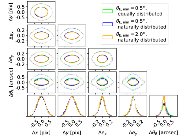
Figure 7: Comparison of the performance of the three networks described in Sect. 4. All samples include doubles and quads and a weighting factor of $w_{\theta_{\text{E}}}=5$, but different Einstein radius distributions or lower limits on the Einstein radius (see legend). In the bottom row are shown the normalized histograms of the difference between predicted values and ground truth for the five parameters and above the 2D correlations distribution: 1$\sigma$ contour (solid line) and 2$\sigma$ contour (dotted line).

Finally, we show in Figure 8 the difference in Einstein radii as a function of the logarithm of the ratio between lensed source intensity $I_{\text{s}}$ and lens intensity $I_{\text{l}}$ determined in the $i$ band, which we hereafter refer to as the brightness ratio. In the top right panel, we show the distribution of the brightness ratio. The lens intensity is defined as the sum of all the pixel values in the 64 pixels $\times$ 64 pixels cutout of the lens such that it is slightly overestimated due to light contamination from surrounding objects. The distribution peaks around $-2$ in logarithm to basis 10, which means that the lensed source flux is a factor 100 below that of the lens. The bottom left plot shows the median with 1$\sigma$ values of the Einstein radius differences for each brightness ratio bin. Focussing on the blue curve for this section, we find a bias in the Einstein radius which is driven by the small lensing systems with $\theta_{\text{E}}\lesssim 0.8\arcsec$ (compare Figure 6). Excluding these small lensing systems, we show the corresponding plot in the lower right panel. With this limitation, we no longer find a bias, and obtain a median with 1$\sigma$ values of $0.00_{-0.14}^{+0.17}$$\arcsec$ for the Einstein radius difference. We find a slight improvement of the performance with increasing brightness ratio for both the full sample (bottom left panel) and the sample with $\theta_{\text{E}}>0.8\arcsec$ (bottom right panel).

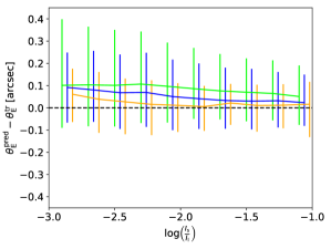
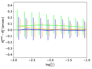
Figure 8: Comparison of the performance of the three networks described in Sect. 4. All samples include doubles and quads and a weighting factor of $w_{\theta_{\text{E}}}=5$, but different Einstein radius distribution or lower limits on the Einstein radius as indicated in the legend (upper left). The upper right panel shows the histogram of the brightness ratio of lensed source and lens. The bottom panel shows for the full sample (left) and limited to $\theta_{\text{E}}>0.8\arcsec$ (right) the difference in Einstein radius as a function of the brightness ratio with the 1$\sigma$ values. Shown are the Einstein radius difference in the range $-3\leq\text{log}\left(\frac{I_{s}}{I_{l}}\right)\leq-1$ (white area in the histogram) where there are enough data points, and the blue and orange bars have been shifted slightly to the right for better visualization.

To further improve the network performance for wide-separation lenses, we train separate networks for lens systems with Einstein radius $\theta_{\text{E}}>2.0\arcsec$ in Sect. 4.2, and for lens systems where we artificially boost the number of lenses at the high end of $\theta_{\text{E}}$ in Sect. 4.3.

4.2 Naturally distributed Einstein radii with lower limit $2.0\arcsec$

Since the network presented in Sect. 4.1 cannot easily recover a large Einstein radius ($\theta_{\text{E}}\gtrsim 2\arcsec$), we test the performance of a network specialized for the high end of the distribution and set the lower limit to $\theta_{\text{E,min}}=2\arcsec$. Because of the higher limit on the Einstein radii, the velocity dispersion (see orange histogram in Figure 1, bottom) is shifted towards the high end, which corresponds to more massive galaxies. We also find that the lens and source redshifts (orange histograms in Figure 1 and Figure 2, respectively) tend to slightly higher values. Since we use the natural distribution of Einstein radii as in Sect. 4.1, the image-separation distribution is again bottom-heavy and the number of mock lens systems is smaller (25,623), as shown in Figure 9. From the blue (predicted) histogram, we see that the true distribution (red histogram) is well recovered.

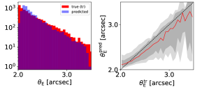
Figure 9: Network performance on the Einstein radius under the assumption of a smalles Einstein radius $\theta_{\text{E,min}}$ of $2.0\arcsec$. The left panel shows the histograms of the ground truth (tr) in red and of the predicted values in blue. The right panel is a 1:1 plot of predicted against true Einstein radius. The red line shows the median of the distribution and the gray bands give the 1$\sigma$ and 2$\sigma$ ranges. For both plots 30 bins over the plotting range are used.

In the right panel of Figure 9 we show the correlation of predicted and true Einstein radii. The red line, which follows quite well the diagonal dashed line, shows the median. The gray shaded regions show the $1\sigma$ and $2\sigma$ regions. We find that the network performs much better for $\theta_{\text{E}}\sim 2\arcsec$ than for the network trained in the full range (Sect. 4.1). However, this is again due to the number of lens systems that decreases towards $\theta_{\text{E}}\sim 4\arcsec$, and the scatter that increases dramatically for the high end of the data set.

We further show 1D and 2D probability distributions for this network in Figure 7 (orange) as well as the histogram of the brightness ratio, and the difference of the Einstein radii as function of the brightness ratio in Figure 8. While the performance for the lens center and complex ellipticity is very similar to the network presented in Sect. 4.1, we achieve an improvement for the Einstein radius. This is expected as the network is specifically trained for lens systems with large image separation. As we see from Figure 8, the larger systems do not have a higher brightness ratio on average as one might expect. As we have already seen, the network performs notably better on the Einstein radii over the whole brightness ratio range. We no longer overpredict the Einstein radius for $\log\left(\frac{I_{\text{s}}}{I_{\text{l}}}\right)\gtrsim-2.5$, and the 1$\sigma$ values are smaller as well.

4.3 Uniformly distributed Einstein radii with lower limit $0.5\arcsec$

Because of the extreme decrease in the number of systems towards large image separation, we test a network trained on a more uniformly distributed sample. For this, we generate more lens systems with high image separation by rotating the lens image by $n\pi/2$ with $n\in[0,1,2,3]$. Here we do not reuse the same lens in the same rotation to avoid producing multiple images of lens systems that are too similar. We note that the background source and position are always different such that the lensing effect varies (see Sect. 2 for further details on the simulation procedure). We limit the sample to a maximum of 8,000 lens systems per $0.1\arcsec$ bin resulting in a sample of 140,812 lens systems. This results in a more uniform distribution, though the bins with the largest image separation still have fewer lens systems since it is very difficult, and a very seldom occurrence, to obtain a lensing configuration with an image separation above $\sim$$2.5\arcsec$ due to the mass distribution of galaxy-scale lenses. The biggest image separation within this sample is $\sim$$4.5\arcsec$, which is about $10\%$ lower than the upper limit of 5$\arcsec$ that we set for our simulations (see Sect. 2.3). The redshift distributions, shown as green histograms in Figure 1 and Figure 2, are similar to that of the naturally distributed sample (blue), whereas the lens velocity dispersions (Figure 1, bottom panel) tend to be higher (i.e., more massive galaxies), as expected.

Similar to the networks trained with natural Einstein radius distribution (see Sect. 4.1 and Sect. 4.2), in Figure 10 we show histograms (left column) and a 1:1 comparison (right column), but now for all five SIE parameters (from top to bottom for the lens center $x$ and $y$, the complex ellipticity $e_{x}$ and $e_{y}$, and the Einstein radius $\theta_{\text{E}}$). For this network we obtain a median value with 1$\sigma$ scatter of $(0.00^{+0.30}_{-0.30})\arcsec$ for $\Delta x$, $(0.00^{+0.30}_{-0.29})\arcsec$ for $\Delta y$, $-0.01^{+0.08}_{-0.09}$ for $\Delta e_{\text{x}}$, $0.00^{+0.08}_{-0.09}$ for $\Delta e_{\text{y}}$, and $(0.07^{+0.29}_{-0.12})\arcsec$ for the Einstein radius $\Delta\theta_{\text{E}}$. Comparing the performance on the Einstein radius to the network from Sect. 4.1 with a natural Einstein radius distribution, we see a significant improvement for the systems with larger image separation. Therefore, we can confirm that the underprediction of the Einstein radius in Sect. 4.1 is due to the relatively small number of large-$\theta_{\text{E}}$ systems in the training data. On the other hand, based on this plot the new network seems to be slightly worse for the low-image separation systems. It tends to overpredict the Einstein radius at $\theta_{\text{E}}\lesssim 2.0\arcsec$ such that when we limit to $\theta_{\text{E}}>0.8\arcsec$ as in Sect. 4.1, we only get a slight improvement in reducing the scatter and obtain $\Delta\theta_{\text{E}}=(0.07_{-0.08}^{+0.25})\arcsec$. Therefore, it turns out that the performance depends sensitively on the training data distribution.

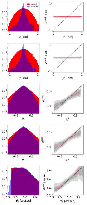
Figure 10: Network performance under the assumption of a lowest Einstein radius $\theta_{\text{E,min}}$ of $0.5\arcsec$ but a uniform distribution up to $\sim 2\arcsec$. The left panel shows histograms of the ground truth (tr) in red and of the predicted values in blue. The right panel shows a direct comparison of the predicted against the true value. From top to bottom are the five different model parameters, lens center $x$ and $y$, complex elliptcity $e_{x}$ and $e_{y}$, and Einstein radius $\theta_{\text{E}}$. For all plots 30 bins over the plotting range are used.

We find a very similar performance on the lens center and ellipticity as for the network with the natural distribution (see Sect. 4.1). This is expected since the only difference is the distribution in Einstein radii. This can be further visualized with the 1D and 2D probability contours in Figure 7 (green) that show that overall this network performs very similarly to the network trained on the naturally distributed sample (blue). For all three networks we find minimal correlation between the different parameters.

In analogy to the previously presented networks, we show in Figure 8 the histogram of the brightness ratio and the Einstein radius differences as function of the brightness ratio for this network. While the distribution matches that from the sample with naturally distributed Einstein radius, we overpredict the Einstein radius more than before. This is related to the overprediction at smaller Einstein radii (see Figure 10), which comes from weighting higher the fraction of systems with larger image separation. We still underestimate the Einstein radius at the very high end, as already noted, but this is negligible for the overall performance compared to the amount of overestimated systems as we still have a factor of $\sim$ 100 more of them in our sample. This is the reason why the network tends to overpredict more strongly than that trained on the naturally distributed sample (Sect. 4.1, and blue lines in Figure 7 and Figure 8).

Finally, we show the loss curve in Figure 11. The training losses (dotted lines) and validation losses (solid lines) in different colors correspond to the five different cross-validation runs. Additionally, we give the mean of the validation curves with a black solid line. This line is used to obtain the best epoch, which in this specific case is epoch 122 (vertical line). The corresponding loss is 0.0528 obtained with Eq. 6.

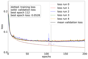
Figure 11: Loss curve of our best network under the assumption of equally distributed Einstein radii. The training loss is shown as dotted lines in five different colors for the five different cross-validation runs. In the same colors the validation loss is shown as solid lines together with the black curve, which is the average of the five validation curves from the cross-validation runs. From the minimum in the black curve, shown as the vertical gray line, the best epoch is found.

From the loss curve we see that the network does not overfit much to the training set since the validation curves do not increase much for higher epochs, but still enough to define the optimal epoch to terminate the final training. This is a sign that drop-out is not needed, which is supported by additional tests (see Sect. 3).

5 Further network tests

In addition to the networks described in Sect. 4, where we mainly investigated the effect of the Einstein radius distribution, in this section we discuss further tests on the training data set.

5.1 Data set containing double or quads only

We considered a specialized network for one of the two strong lensing options and limited our sample to either doubles or quads, where the image multiplicity is based on the centroid of the source (as the spatially extended parts of the source could have different image multiplicities depending on their positions with respect to the lensing caustics). In the case where we limited the sample to doubles only, we did our standard grid search for the different hyperparameter combinations for two samples with naturally distributed Einstein radii above $0.5\arcsec$ and above $2.0\arcsec$. With these networks we found no notable difference compared to the sample containing both doubles and quads (see Sect. 4.1 and Sect. 4.2), which was expected as the doubles dominate the sample including both doubles and quads by a factor of around 20-30 (for the different networks depending on the lower limit of the Einstein radii).

When we limited the sample to quads only, we performed our grid search again for the different hyperparameter combinations of both samples with naturally distributed Einstein radii above $0.5\arcsec$ and above $2.0\arcsec$ and also with equally distributed Einstein radii. Since the chance of obtaining four images is smaller than the chance of observing two images based on the necessary lensing configuration probability, the sample sizes are smaller with 42 063, 19 176, and 28 398 lensing systems. Therefore, the output has to be considered with care as this is much lower than typically used for such a network.

It turns out that these networks perform equally well on the lens center and ellipticity but better for the Einstein radius shown in Figure 12. By comparing this plot to Figure 10, we find the main improvement that the 1$\sigma$ and 2$\sigma$ scatters are substantially reduced and with smaller bias for systems with larger $\theta_{\rm E}$. An improvement on the Einstein radius is expected as the network gets the same information for the lens, but more for the lensed arcs. Even if one image is now too faint to be detected or is too blended with the lens there are three images from the quad left over to provide information on the Einstein radius.

To increase the sample we simulated a new quads-only batch with the source brightness boosted by one magnitude, which resulted in a $\sim 1.5$ times larger sample than before. This is still small compared to the other double or mixed samples. Now we have a brightness ratio peak at $\log\left(\frac{I_{\text{s}}}{I_{\text{l}}}\right)\sim-1.5$ instead of $\sim-2.0$ (as shown in Figure 8). The performance obtained with this trained network (the loss is 0.0673 for the network with $w_{\theta_{\text{E}}}=5$) is still similar to that for the quads-only network without magnitude boost (the loss is 0.0688) and no significant performance difference is observed for the individual parameters.

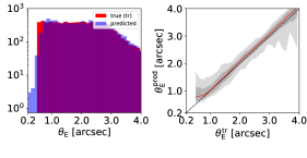
Figure 12: Network performance under the assumption of a lowest Einstein radius $\theta_{\text{E,min}}$ of $0.5\arcsec$ but a uniform distribution with quadruply lensed images. The left panel shows histograms of the ground truth (tr) in red and of the predicted values in blue. The right panel is a 1:1 plot of predicted against true Einstein radius. For both plots 30 bins over the plotting range are used.

5.2 Comparison to lens galaxy images only

As further proof of the network performance on the Einstein radius, we test how well the network is able to predict the parameters from images of only the lens galaxies (i.e., without lensed arcs). As expected, the network performs similarly well for the lens center and axis ratio, but much worse for the Einstein radius with a 1$\sigma$ value of $0.41\arcsec$. This shows us that the arcs are bright enough and sufficiently deblended from the lens galaxies to be detectable by the CNN.

6 Prediction of lensed image position(s) and time-delay(s)

After obtaining a network for different data sets (see Table 1), we compared the true and predicted parameter values directly. Since the main advantage of the network is the computational speed-up compared to recent methods and the fully automated application, the network is very useful for planning follow-up observations. This needs to be done quickly in case there is, for instance, a SN or a short-lived transient occurring in the background source. We explore below how accurately we can predict the positions and time-delays of the next appearing SN images.

We used the predicted SIE parameters from the networks to predict the image positions and time-delays and compared them to those obtained with the ground-truth SIE model parameter values. This gives us a better understanding of how well the network performs and if the obtained accuracy is sufficient for such an application. For this comparison we computed the image positions of the true source center based on the true SIE parameters obtained by the simulation for the sytsems of the test set (hereafter true image positions). After removing the central highly demagnified lensed image as this would not be observable (given its demagnification and the presence of the lens galaxy in the optical–infrared), we computed the time-delays for these systems (hereafter true time-delays $\Delta t^{\text{tr}}$) by using the known redshifts and our assumed cosmology. Based on these true image positions and time-delays, we were able to select the first-appearing image and use its true image position to predict the source position with our predicted SIE mass model. This source position was then used to predict the image positions (hereafter predicted image positions) of the next-appearing SN images based on the SIE parameter values predicted with our modeling network. The predicted image positions were then used to predict the time-delays (hereafter predicted time-delays $\Delta t^{\text{pred}}$) with the network predicted SIE parameter. We directly compared the image positions and time-delays that we obtained with the true and with the network predicted SIE parameters when we had the same number of multiple images. If the number of images did not match, which happened for 7.8% of the sample used for the network with equally balanced Einstein radii distribution containing double and quads, we omitted the candidate from this analysis as a fair comparison was not possible. Since we always remove the central image, we obtain for a double and quad, respectively, two and four images and one and three time-delays. Since the time-delays can be very different, we also compared the fractional difference between the true and predicted time-delays with respect to the true time-delays.

We chose again the three main networks from Sect. 4 for this comparison; they are shown in Figure 13. All three sets contain quads and doubles, and assume a loss weighting factor of 5 for the Einstein radius. The first set assumes a lower limit on the Einstein radius of 0.5″(blue), the second a lower limit of 2″(yellow), and the third a lower limit of again 0.5″ but with a uniform distribution on the Einstein radii instead of the natural distribution following the lensing probability (green). We plot the quantities as a function of the brightness ratio $\log\left(\frac{I_{\text{s}}}{I_{\text{l}}}\right)$ in analogy to Figure 7 and Figure 8.

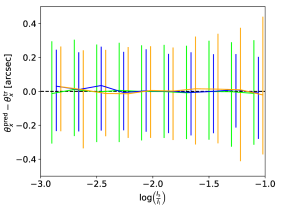
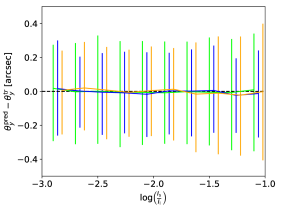
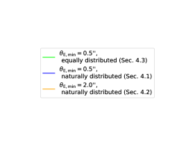
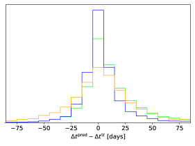
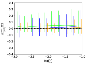
Figure 13: Precision of model network predictions as a function of the lens and lensed source brightness ratio in the range $-3\leq\text{log}\left(\frac{I_{s}}{I_{l}}\right)\leq-1$ for the three networks presented in Sect. 4 applied to the restricted sample with $\theta^{\text{tr}}_{\text{E}}>0.8\arcsec$. The upper row shows the image position offset for the $x$ coordinate (left) and $y$ coordinate (right). In the middle panel is the legend (left) and a histogram of the difference in time-delay (right), while in the bottom row is shown the fraction of the time-delay difference and the true time-delay (left) and the time-delay difference (right). The curves show the median and the vertical bars the 1$\sigma$ values. The blue and orange bars have been shifted slightly to the right for better visualization.

In detail, Figure 13 contains in the upper row the median difference in the image position for the $x$ coordinate (left) and $y$ coordinate (right) with the 1$\sigma$ value per brightness ratio bin, where only the additional image positions are taken into account as the first reference image is known, and thus they do not need to be predicted. We obtain for all three networks a median offset of nearly zero independent of the brightness ratio and whether we limit further in Einstein radii or not. The 1$\sigma$ values are around $0.25\arcsec$, corresponding to $\sim 1.5$ pixels. Explicitly, we find for the equally distributed sample applied to $\theta_{\text{E}}>0.8\arcsec$ a median image position offset of $(0.00_{-0.29}^{+0.29})\arcsec$ and $(0.00_{-0.31}^{+0.32})\arcsec$ for the $x$ and $y$ coordinate, respectively. Interestingly, the 1$\sigma$ values are slightly larger for quads than doubles as we would have expected that quads provide more information to constrain the SIE parameter values, and thus predict the image positions better. The reason for this is probably because quads generally have higher image magnification than doubles, and image offsets are larger with higher magnification.

The middle row of Figure 13 shows the legend (left) and a histogram of the difference between the predicted time-delay $\Delta t^{\text{pred}}$ and the true time-delay $\Delta t^{\text{true}}$. The bottom row shows the difference in time-delay divided by the absolute value of the true time-delay per brightness ratio bin (left) and the difference of the time-delays again per brightness ratio bin (right). In terms of time-delay difference, the network trained on the natural distribution (blue) performs better than that with uniform distribution (green), but especially for the network trained for lens systems with large Einstein radius (orange) we obtain notable differences. In detail, we obtain a median with 1$\sigma$ value for the naturally distributed sample (blue; see Sect. 4.1) for the time-delay difference of $2_{-6}^{+18}$ days and a fractional time-delay difference of $0.05_{-0.09}^{+0.47}$. Since we find a strong correlation between the offset in the Einstein radius and the time-delay offset (see Figure 14), we exclude again the very small Einstein radii systems ($\theta_{\text{E}}^{\text{tr}}<0.8\arcsec$) and obtain for the time-delay difference $1_{-11}^{+18}$ days and for the fractional difference $0.01_{-0.12}^{+0.19}$. For the equally distributed sample (green; see Sect. 4.3) we obtain, with $\theta_{\text{E}}>0.5\arcsec$ and $\theta_{\text{E}}>0.8\arcsec$, respectively, for the time-delay difference $7_{-6}^{+38}$ and $6_{-8}^{+36}$ days and for the fractional time-delay difference $0.06_{-0.05}^{+0.45}$ and $0.04_{-0.05}^{+0.27}$. This restriction is easily applicable in practice since individual lensing systems are only followed up at a given time, and it is possible to check by looking at the image of the individual system whether the Einstein radius is $>$$0.8\arcsec$. Depending on the predicted time-delay, the model can be further improved by using traditional manual maximum likelihood modeling methods to verify the predicted time-delay.

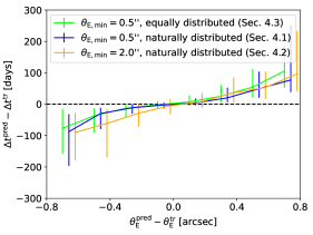
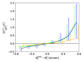
Figure 14: Correlation between Einstein radius offset in the range $-0.8\arcsec\leq\theta_{\text{E}}^{\text{pred}}-\theta_{\text{E}}^{\text{tr}}\leq 0.8\arcsec$ and time-delay difference (left panel) or fractional time-delay difference (right panel) by applying the different networks to their samples after limiting to $\theta_{\text{E}}^{\text{tr}}>0.8\arcsec$. The blue and orange bars have been shifted slightly to the right for better visualization.

The fractional offset in the predicted time-delays of $0.04_{-0.05}^{+0.27}$ that we achieve with our CNN for systems with $\theta_{\text{E}}>0.8\arcsec$ for the uniformly distributed $\theta_{\rm E}$ sample (i.e., with a symmetrized scatter of $\sim$$16\%)$ is close to the limit that would be achievable even with detailed and time-consuming MCMC models of ground-based images. This is because the assumption of the SIE introduces additional uncertainties on the predicted time-delays in practice, even though detailed MCMC models of images would typically yield more precise and accurate estimates for the SIE parameters than our CNN. While galaxy mass profiles are close to being isothermal, the intrinsic scatter in the logarithmic radial profile slope $\gamma^{\prime}$ (where the 3D mass density $\rho(r_{\rm 3D})\propto r_{\rm 3D}^{-\gamma^{\prime}}$) is around $\pm 0.15$, translating to $\sim\,15\%$ scatter in the time-delays (e.g., Koopmans et al., 2006; Auger et al., 2010; Barnabè et al., 2011). In other words, if a lens galaxy has a power-law mass slope of $\gamma^{\prime}=2.1$, then our assumed SIE mass profile (with $\gamma^{\prime}=2.0$) for it would predict time-delays that are $\sim$$10\%$ too high (e.g., Wucknitz, 2002; Suyu, 2012). While constraining the profile slope $\gamma^{\prime}$ with better precision than the intrinsic scatter for individual lenses is possible, this would require high-resolution imaging from space or ground-based adaptive optics (e.g., Dye & Warren, 2005; Chen et al., 2016). Given the difficulties of measuring the power-law mass slope $\gamma^{\prime}$ from seeing-limited ground-based images of lens systems (although see Meng et al., 2015, for the optimistic scenario when various inputs are known perfectly such as the point spread function), we conclude that our network prediction for the delays has uncertainties comparable to that due to the unknown $\gamma^{\prime}$. We expect these two sources of uncertainties to be the dominant ones in ground-based images.

We also find a decrease in the performance with increase in brightness ratio, which is in the first instance counterintuitive. If we consider the fractional offset in the left panel, we see a better performance for the sample with an Einstein radius lower limit of $\theta_{\text{E,min}}=2\arcsec$ (orange), especially in terms of the 1$\sigma$ scatter, when compared to the other two networks. This $\theta_{\text{E,min}}=2\arcsec$ network also has minimal bias, as shown by the median line. This is understandable as the time-delays are longer for systems with a bigger Einstein radius, and therefore the fractional uncertainty is smaller. The accuracy in time-delay difference (lower right plot) is good, although the 1$\sigma$ scatter is quite large, $\sim$$20$ days. With this reasoning, we can also understand the worse performance of the equally distributed sample (green) compared to the naturally distributed sample (blue) as it contains a much higher fraction of systems with bigger image separation. As a higher brightness ratio ($\log(I_{\rm s}/I_{\rm l}$)) tends to be associated with systems with higher $\theta_{\rm E}$, the prediction of delays thus has larger scatter, as shown in the bottom right panel. Moreover, we note that we find a better performance for doubles than quads, probably because of smaller image separation and shorter time-delays of quads.

During this evaluation of the networks we should keep in mind that the main advantage of these networks is the run time: we need only a few seconds to estimate the SIE model parameters, the image positions, and the corresponding time-delays. Therefore, it is expected that we do not reach the accuracy of current modeling techniques using MCMC sampling which can take weeks. Nonetheless, the network results can serve as input to conventional modeling and can help speed up the overall modeling.

7 Comparison to other modeling codes

There are already several modeling codes developed, and they can be separated into two main groups. The state-of-the-art codes that rely on MCMC sampling have been widely tested and used for most of the modeling so far. The advantage of such codes are their flexibility in image cutout size or pixel size and also in terms of profiles to describe the lens light or mass distribution. With the advantage of the variety of profiles comes the disadvantage that the codes require a lot of user input which limit the applicability of such codes to a very small sample, or specific lensing systems that are modeled. Moreover, based on the MCMC sampling of the parameter space is very computationally intensive, and thus can take up to weeks per lens system, although some steps can be parallelized and run on multiple cores.

Since the number of known lens systems has grown in the past few years and will increase substantially with upcoming surveys like LSST and Euclid, the codes used to analyze individual lens systems will no longer be sufficient. Thus, the modeling process must be more automated and a speed-up will be necessary. While some newer codes (e.g., Nightingale et al., 2018; Shajib et al., 2019; Ertl et al., in prep.) are automating the modeling steps to minimize the user input, they still rely on sampling the parameter space such that the run time remains on the order of days or weeks, and some user input per lens system. With these codes it should be possible to obtain results that are comparable with the current interactive modeling procedure.

The second new kind of modeling is based on machine learning such as that used in this work. The first network for modeling strong lens systems was presented by Hezaveh et al. (2017). While they use Hubble Space Telescope data quality, we use ground-based HSC images with similar quality to those used by Pearson et al. (2019) as most of the newly detected lens systems will be in first instance observed with ground-based facilities. Moreover, Hezaveh et al. (2017) suggest first removing the lens light and then only modeling the arcs with the network. Given the differences in the data quality, number of filters, and modeling procedure between Hezaveh et al. (2017) and our work, we cannot further compare the performance fairly.

Pearson et al. (2019) consider modeling with and without lens light subtraction, but found no notable difference; thus, we only consider modeling the lens system without an additional step to remove the lens light. Since we provide the image in four different filters, the network is able to distinguish internally between the lens galaxy and the surrounding arcs. In contrast to Pearson et al. (2019), we use the SIE profile with all five different parameters, while they only predict three parameters: axis ratio, position angle (equivalent to our complex ellipticity), and the Einstein radius. Moreover, they completely mock up their training data, assume a very conservative threshold of S/N$>$20 in at least one band, and do not include neighboring galaxies that can confuse the CNN; instead, we are more realistic by using real observed images as input for the simulation pipeline. We further assume an offset between lens mass distribution and lens light distribution, which complicates the CNN parameter inference further as the network has to predict the mass distribution only from the images. This way we have more realistic lens light and mass distributions and also include neighboring objects which the network has to learn to distinguish from the lensing system. Pearson et al. (2019) make use of a CNN (the same type of network that we use, and also Hezaveh et al. 2017), but they use slightly smaller input cutouts ($57\times 57$ pixels) and a different network architecture (six convolutional layers and two FC layers) than ours.They investigated mostly the effect of using a different number of filters and whether to use lens light subtraction, whereas we investigate the effect on the underlying samples and a simulation with real observed images, which means that we do not have a scenario that assumes the exact same properties. The closest scenario, from Pearson et al. (2019) the results from LSST-like $gri$ images including lens light and our results based on HSC $griz$ images with naturally distribution of the Einstein radii, shows that both networks are very similar in their overall performance.The reason that the performance on the Einstein radius by Pearson et al. (2019) is better and that they do not suffer from the same biases in $\theta_{\text{E}}^{\text{pred}}$, even with a non-flat $\theta_{\text{E}}^{\text{tr}}$ distribution in their simulations, is perhaps because they use idealized simplistic simulations (high S/N, well-resolved systems, no neighbors).

There are also other recent publications related to strong lens modeling with machine learning. Bom et al. (2019) suggest a new network that predicts four parameters: the Einstein radius $\theta_{\text{E}}$, the lens redshift $z_{\text{d}}$, the source redshift $z_{\text{s}}$, and the related quantity of the lens velocity dispersion $v_{\text{disp}}$. They adapt, as we do, a SIE profile to mock up their training data with an image quality similar to that from the Dark Energy Survey. Comparing their performance on the Einstein radius (Figure 8, left panel, assuming $\theta_{\text{E}}^{\text{tr}}$ on the $x$-axis and $\theta_{\text{E}}^{\text{pred}}$ on the $y$-axis) to our performance with the natural distribution (Figure 6), we find a similar trend. Both networks slightly overpredict at the very low end and underpredict at the high end. If we compare this to the network with equal distribution, we see a clear improvement of our network on the median line for $\theta_{\text{E}}\sim 2-3\arcsec$. Since this code only provides the Einstein radius instead of a full SIE model, the applicability is somewhat limited.

Madireddy et al. (2019) suggest a modular network to combine lens detection and lens modeling which to date have been done with complete independent networks. In detail, they have four steps. The first is to reduce the background noise (so-called image denoising), followed by a lens light subtracting step (the deblending step), before the next network decides whether this is a lens system or not. If it detects the input image to be a lens, the module is called to predict the mass model parameter values. Each module of the network is a very deep network and both modules for detection and modeling make use of the residual neural network (ResNet) approach. They use a sample of 120,000 images, with 60,000 lenses and 60,000 non-lenses, and split this into 90% and 10% for the training and test set, respectively, without making use of the cross-validation procedure. Madireddy et al. (2019) use, as do Pearson et al. (2019), completely mocked-up images based on a SIE profile with fixed centroid to the image center such that the modeling module predicts three quantities, Einstein radius, and the two components of the complex ellipticity. Based on the different assumptions a direct comparison of the lens modeling performance is not possible. However, we see that the performance is typical for the current state of CNNs based on Pearson et al. (2019).

Comparing the network-based modeling to the traditional model using MCMC on a concrete sample is difficult as first we have to obtain the mass models for that sample with both methods. However, in general it is expected that the MCMC models are typically more precise than those obtained with neural networks because of the interactive and individual modeling procedure. In the MCMC modeling, the image residuals can be inspected to see whether the model is good and trustworthy, or if the parameters need to be refined further and different mass profile adopted (e.g., SIE plus external shear). In contrast, the fully automated procedure with CNN does not inspect the individual images and residuals in detail. However, for upcoming surveys like LSST it is impossible to model all the expected $\sim$$100,000$ lens systems in the traditional MCMC way systematically given the computational time required. The only way to analyze the entire LSST lens sample will be a fully automated, fast procedure where a small fraction of outliers and (probably) slightly higher uncertainties are acceptable. Therefore, the substantial speed-up is a very important advantage of CNN modeling, as we can process one lens systems with our CNN in fractions of a second compared to weeks or months with MCMC methods. If one is interested in a specific lens system such as a lensed SN, one can consider starting with a CNN to get a good initial mass model and then refining with traditional methods to achieve a good balance between speed and accuracy.

8 Summary and conclusion

In this paper, we presented a convolutional neural network to model in a fully automated way and very quickly the mass distribution of galaxy-scale strong lens systems by assuming a SIE profile. The network is trained on images of lens systems generated with our newly developed code that takes real observed galaxy images as input for the source galaxy (in our case from the Hubble Ultra Deep Field), lenses the source onto the lens plane, and adds it to another real observed galaxy image for the lens galaxy (in our case from the HSC SSP survey). We chose the HSC images as lenses and adopted their pixel sizes of $0.168\arcsec$ as this is similar to the data quality expected from LSST. With this procedure we simulated different samples to train our networks where we distinguish between the lens types (quads+doubles, doubles-only, and quads-only) and on the lower limit of the Einstein radius range. Since we find a strong dependence on the Einstein radius distribution, we also consider a uniformly distributed sample and also a weighting factor of 5 for the Einstein radius’ contribution to the loss. With this we obtain eight different samples for each of the two different weighting assumptions summarized in Table 1.

For each sample we then perform a grid search to test different hyperparameter combinations to obtain the best network for each sample, although we find that the CNN performance depends much more critically on the assumptions of the mock training data (e.g., quads, doubles, both, or Einstein radius distribution) rather than on the fine-tuning of hyperparameters. From the different networks presented in Table 1, we find a good improvement for the networks trained with quads-only compared to the networks trained on both quads and doubles. If the system type is known, we therefore recommend using the corresponding network. Since the Einstein radius is a key parameter, we weighted its loss higher than for the others and, although the minimal validation loss is higher, we advocate these networks for modeling HSC-like lenses. With the network trained on both quads and doubles with the uniform distributed sample of $\theta_{\text{E}}$ $>0.5\arcsec$, we obtain for the five SIE parameters a median with 1$\sigma$ value as follows: $\Delta x=(0.00^{+0.30}_{-0.30})\arcsec$, $\Delta y=(0.00^{+0.30}_{-0.29})\arcsec$, $\Delta\theta_{\text{E}}=(0.07^{+0.29}_{-0.12})\arcsec$, $\Delta e_{x}=-0.01^{+0.08}_{-0.09}$, and $\Delta e_{y}=0.00^{+0.08}_{-0.09}$.

After comparing the network performance on the SIE parameter level, we tested the network performance on the lensed image and time-delay level. For this we used the first appearing image of the true mass model to predict the source position based on the predicted SIE parameter. From this source position and the network predicted SIE parameters, we then predicted the other image position(s) and time-delay(s). We find for the sample with doubles and quads a uniform distribution in Einstein radii and a weighting factor $w_{\theta_{\text{E}}}$ of five by applying the network to $\theta_{\text{E}}>0.8\arcsec$ an average image offset of $\Delta\theta_{x}=(0.00_{-0.29}^{+0.29})\arcsec$ and $\Delta\theta_{y}=(0.00_{-0.31}^{+0.32})\arcsec$, while we achieve the fractional time-delay difference of $0.04_{-0.05}^{+0.27}$.

This is very good given that we use a simple SIE profile and need only a few seconds per lens system in comparison to state-of-the-art methods that require at least days and some user input per lens system. We anticipate that fast CNN modeling such as the one developed here will be crucial for coping with the vast amount of data from upcoming imaging surveys. For future work, we suggest investigating further into creating even more realistic training data (e.g., allowing for an external shear component in the lens mass model) and also exploring the effect of deeper or more complex network architectures. The outputs of even the network presented here can be used to prune down the sample for specific scientific studies, which can then be followed up with more detailed conventional mass modeling techniques.

References

- Aihara et al. (2019) Aihara, H., AlSayyad, Y., Ando, M., et al. 2019, PASJ, 106
- Auger et al. (2010) Auger, M. W., Treu, T., Bolton, A. S., et al. 2010, ApJ, 724, 511
- Barkana (1998) Barkana, R. 1998, ApJ, 502, 531
- Barnabè et al. (2011) Barnabè, M., Czoske, O., Koopmans, L. V. E., Treu, T., & Bolton, A. S. 2011, MNRAS, 415, 2215
- Barnabè et al. (2012) Barnabè, M., Dutton, A. A., Marshall, P. J., et al. 2012, MNRAS, 423, 1073
- Baron & Poznanski (2017) Baron, D. & Poznanski, D. 2017, MNRAS, 465, 4530
- Beckwith et al. (2006) Beckwith, S. V. W., Stiavelli, M., Koekemoer, A. M., et al. 2006, AJ, 132, 1729
- Belokurov et al. (2007) Belokurov, V., Evans, N. W., Moiseev, A., et al. 2007, ApJ, 671, L9
- Bertin & Arnouts (1996) Bertin, E. & Arnouts, S. 1996, A&AS, 117, 393
- Bolton et al. (2006) Bolton, A. S., Burles, S., Koopmans, L. V. E., Treu, T., & Moustakas, L. A. 2006, ApJ, 638, 703
- Bom et al. (2019) Bom, C., Poh, J., Nord, B., Blanco-Valentin, M., & Dias, L. 2019, arXiv e-prints, arXiv:1911.06341
- Bom et al. (2017) Bom, C. R., Makler, M., Albuquerque, M. P., & Brand t, C. H. 2017, A&A, 597, A135
- Bonvin et al. (2017) Bonvin, V., Courbin, F., Suyu, S. H., et al. 2017, MNRAS, 465, 4914
- Brownstein et al. (2012) Brownstein, J. R., Bolton, A. S., Schlegel, D. J., et al. 2012, ApJ, 744, 41
- Cañameras et al. (2020) Cañameras, R., Schuldt, S., Suyu, S. H., et al. 2020, arXiv e-prints, arXiv:2004.13048
- Cabanac et al. (2007) Cabanac, R. A., Alard, C., Dantel-Fort, M., et al. 2007, A&A, 461, 813
- Chan et al. (2020) Chan, J. H. H., Suyu, S. H., Sonnenfeld, A., et al. 2020, A&A, 636, A87
- Chen et al. (2019) Chen, G. C. F., Fassnacht, C. D., Suyu, S. H., et al. 2019, MNRAS, 490, 1743
- Chen et al. (2016) Chen, G. C. F., Suyu, S. H., Wong, K. C., et al. 2016, MNRAS, 462, 3457
- Chirivì et al. (2020) Chirivì, G., Yıldırım, A., Suyu, S. H., & Halkola, A. 2020, arXiv e-prints, arXiv:2003.08404
- Collett (2015) Collett, T. E. 2015, ApJ, 811, 20
- Cornachione et al. (2018) Cornachione, M. A., Bolton, A. S., Shu, Y., et al. 2018, ApJ, 853, 148
- Dark Energy Survey Collaboration et al. (2005) Dark Energy Survey Collaboration et al. 2005, arXiv e-prints
- Davies et al. (2018) Davies, L. J. M., Robotham, A. S. G., Driver, S. P., et al. 2018, MNRAS, 480, 768
- Dye et al. (2018) Dye, S., Furlanetto, C., Dunne, L., et al. 2018, MNRAS, 476, 4383
- Dye & Warren (2005) Dye, S. & Warren, S. J. 2005, ApJ, 623, 31
- Eales et al. (2015) Eales, S., Fullard, A., Allen, M., et al. 2015, MNRAS, 452, 3489
- Ertl et al. (in prep.) Ertl et al. in prep.
- Fowlie et al. (2020) Fowlie, A., Handley, W., & Su, L. 2020, arXiv e-prints, arXiv:2006.03371
- Gavazzi et al. (2014) Gavazzi, R., Marshall, P. J., Treu, T., & Sonnenfeld, A. 2014, ApJ, 785, 144
- Goldstein et al. (2019) Goldstein, D. A., Nugent, P. E., & Goobar, A. 2019, ApJS, 243, 6
- Goobar et al. (2017) Goobar, A., Amanullah, R., Kulkarni, S. R., et al. 2017, Science, 356, 291
- Hashim et al. (2014) Hashim, N., De Laurentis, M., Zainal Abidin, Z., & Salucci, P. 2014, arXiv e-prints, arXiv:1407.0379
- Hezaveh et al. (2017) Hezaveh, Y. D., Perreault Levasseur, L., & Marshall, P. J. 2017, Nature, 548, 555
- Huang et al. (2020) Huang, X., Storfer, C., Gu, A., et al. 2020, arXiv e-prints, arXiv:2005.04730
- Inami et al. (2017) Inami, H., Bacon, R., Brinchmann, J., et al. 2017, A&A, 608, A2
- Ivezic et al. (2008) Ivezic, Z., Axelrod, T., Brandt, W. N., et al. 2008, Serbian Astronomical Journal, 176, 1
- Jacobs et al. (2017) Jacobs, C., Glazebrook, K., Collett, T., More, A., & McCarthy, C. 2017, MNRAS, 471, 167
- Jaelani et al. (2020) Jaelani, A. T., More, A., Oguri, M., et al. 2020, MNRAS, 495, 1291
- Jullo et al. (2007) Jullo, E., Kneib, J. P., Limousin, M., et al. 2007, New Journal of Physics, 9, 447
- Kelly et al. (2015) Kelly, P. L., Rodney, S. A., Treu, T., et al. 2015, Science, 347, 1123
- Koopmans et al. (2006) Koopmans, L. V. E., Treu, T., Bolton, A. S., Burles, S., & Moustakas, L. A. 2006, ApJ, 649, 599
- Krywult et al. (2017) Krywult, J., Tasca, L. A. M., Pollo, A., et al. 2017, A&A, 598, A120
- Lanusse et al. (2018) Lanusse, F., Ma, Q., Li, N., et al. 2018, MNRAS, 473, 3895
- Laureijs et al. (2011) Laureijs, R., Amiaux, J., Arduini, S., et al. 2011, arXiv e-prints, arXiv:1110.3193
- Lemon et al. (2018) Lemon, C. A., Auger, M. W., McMahon, R. G., & Ostrovski, F. 2018, MNRAS, 479, 5060
- Loubser et al. (2020) Loubser, S. I., Babul, A., Hoekstra, H., et al. 2020, MNRAS
- Madireddy et al. (2019) Madireddy, S., Li, N., Ramachandra, N., et al. 2019, arXiv e-prints, arXiv:1911.03867
- Maturi et al. (2014) Maturi, M., Mizera, S., & Seidel, G. 2014, A&A, 567, A111
- McGreer et al. (2018) McGreer, I. D., Clément, B., Mainali, R., et al. 2018, MNRAS, 479, 435
- Meng et al. (2015) Meng, X.-L., Treu, T., Agnello, A., et al. 2015, J. Cosmology Astropart. Phys., 2015, 059
- Metcalf et al. (2019) Metcalf, R. B., Meneghetti, M., Avestruz, C., et al. 2019, A&A, 625, A119
- Morningstar et al. (2018) Morningstar, W. R., Hezaveh, Y. D., Perreault Levasseur, L., et al. 2018, arXiv e-prints, arXiv:1808.00011
- Morningstar et al. (2019) Morningstar, W. R., Perreault Levasseur, L., Hezaveh, Y. D., et al. 2019, ApJ, 883, 14
- Nightingale et al. (2018) Nightingale, J. W., Dye, S., & Massey, R. J. 2018, MNRAS, 478, 4738
- Nomoto (1982) Nomoto, K. 1982, ApJ, 257, 780
- Ostrovski et al. (2017) Ostrovski, F., McMahon, R. G., Connolly, A. J., et al. 2017, MNRAS, 465, 4325
- Pakmor et al. (2010) Pakmor, R., Röpke, F., Hillebrandt, W., et al. 2010, in Progenitors and Environments of Stellar Explosions, 62
- Pearson et al. (2019) Pearson, J., Li, N., & Dye, S. 2019, MNRAS, 488, 991
- Perreault Levasseur et al. (2017) Perreault Levasseur, L., Hezaveh, Y. D., & Wechsler, R. H. 2017, ApJ, 850, L7
- Petrillo et al. (2017) Petrillo, C. E., Tortora, C., Chatterjee, S., et al. 2017, MNRAS, 472, 1129
- Planck Collaboration et al. (2018) Planck Collaboration, Aghanim, N., Akrami, Y., et al. 2018, arXiv e-prints, arXiv:1807.06209
- Refsdal (1964) Refsdal, S. 1964, MNRAS, 128, 307
- Riess et al. (2019) Riess, A. G., Casertano, S., Yuan, W., Macri, L. M., & Scolnic, D. 2019, ApJ, 876, 85
- Rizzo et al. (2018) Rizzo, F., Vegetti, S., Fraternali, F., & Di Teodoro, E. 2018, MNRAS, 481, 5606
- Rubin et al. (2018) Rubin, D., Hayden, B., Huang, X., et al. 2018, ApJ, 866, 65
- Rusu et al. (2020) Rusu, C. E., Wong, K. C., Bonvin, V., et al. 2020, MNRAS
- Salmon et al. (2018) Salmon, B., Coe, D., Bradley, L., et al. 2018, ApJ, 864, L22
- Schaefer et al. (2018) Schaefer, C., Geiger, M., Kuntzer, T., & Kneib, J. P. 2018, A&A, 611, A2
- Sciortino et al. (2020) Sciortino, F., Howard, N. T., Marmar, E. S., et al. 2020, arXiv e-prints, arXiv:2006.06798
- Seidel & Bartelmann (2007) Seidel, G. & Bartelmann, M. 2007, A&A, 472, 341
- Shajib et al. (2020) Shajib, A. J., Birrer, S., Treu, T., et al. 2020, MNRAS, 494, 6072
- Shajib et al. (2019) Shajib, A. J., Birrer, S., Treu, T., et al. 2019, MNRAS, 483, 5649
- Shu et al. (2016) Shu, Y., Bolton, A. S., Mao, S., et al. 2016, ApJ, 833, 264
- Shu et al. (2017) Shu, Y., Brownstein, J. R., Bolton, A. S., et al. 2017, ApJ, 851, 48
- Shu et al. (2018) Shu, Y., Marques-Chaves, R., Evans, N. W., & Pérez-Fournon, I. 2018, MNRAS, 481, L136
- Sim et al. (2010) Sim, S. A., Röpke, F. K., Hillebrandt, W., et al. 2010, ApJ, 714, L52
- Sonnenfeld et al. (2018a) Sonnenfeld, A., Chan, J. H. H., Shu, Y., et al. 2018a, PASJ, 70, S29
- Sonnenfeld et al. (2018b) Sonnenfeld, A., Leauthaud, A., Auger, M. W., et al. 2018b, MNRAS, 481, 164
- Sonnenfeld et al. (2015) Sonnenfeld, A., Treu, T., Marshall, P. J., et al. 2015, ApJ, 800, 94
- Strigari (2013) Strigari, L. E. 2013, Phys. Rep, 531, 1
- Suyu (2012) Suyu, S. H. 2012, MNRAS, 426, 868
- Suyu & Halkola (2010) Suyu, S. H. & Halkola, A. 2010, A&A, 524, A94
- Suyu et al. (2012) Suyu, S. H., Hensel, S. W., McKean, J. P., et al. 2012, ApJ, 750, 10
- Suyu et al. (2020) Suyu, S. H., Huber, S., Cañameras, R., et al. 2020, arXiv e-prints, arXiv:2002.08378
- Suyu et al. (2006) Suyu, S. H., Marshall, P. J., Hobson, M. P., & Blandford, R. D. 2006, MNRAS, 371, 983
- Tanoglidis et al. (2020) Tanoglidis, D., Drlica-Wagner, A., Wei, K., et al. 2020, arXiv e-prints, arXiv:2006.04294
- Treu et al. (2011) Treu, T., Dutton, A. A., Auger, M. W., et al. 2011, MNRAS, 417, 1601
- Warren & Dye (2003) Warren, S. J. & Dye, S. 2003, ApJ, 590, 673
- Whelan & Iben (1973) Whelan, J. & Iben, Icko, J. 1973, ApJ, 186, 1007
- Wojtak et al. (2019) Wojtak, R., Hjorth, J., & Gall, C. 2019, MNRAS, 487, 3342
- Wong et al. (2018) Wong, K. C., Sonnenfeld, A., Chan, J. H. H., et al. 2018, ApJ, 867, 107
- Wong et al. (2020) Wong, K. C., Suyu, S. H., Chen, G. C. F., et al. 2020, MNRAS
- Wucknitz (2002) Wucknitz, O. 2002, MNRAS, 332, 951
- Yıldırım et al. (2020) Yıldırım, A., Suyu, S. H., & Halkola, A. 2020, arXiv e-prints, arXiv:1904.07237