Nonlinear steering criteria for arbitrary two-qubit quantum systems

Abstract

Abstract: By employing Pauli measurements, we present some nonlinear steering criteria applicable for arbitrary two-qubit quantum systems and optimized ones for symmetric quantum states. These criteria provide sufficient conditions to witness steering, which can recover the previous elegant results for some well-known states. Compared with the existing linear steering criterion and entropic criterion, ours can certify more steerable states without selecting measurement settings or correlation weights, which can also be used to verify entanglement as all steerable quantum states are entangled.

I Introduction

Quantum steering describes the ability of one observer to nonlocally affect the other observer’s state through local measurements, which was first noted by Einstein, Podolsky and Rosen (EPR) for arguing the completeness of quantum mechanics in 1935 ein , and later introduced by Schrödinger in response to the well-known EPR paradoxsch . After being formalized by Wiseman et al. with a local hidden variable (LHV)-local hidden state model in 2007 wis , quantum steering has attracted increasing attention and been explored widely. Steerable states were shown to be advantageous for tasks involving secure quantum teleportation rei ; ros , quantum secret sharing walk ; kog , one-sided device-independent quantum key distribution bra and channel discrimination pia .

Quantum steering is one form of quantum correlations intermediate between quantum entanglement horo and Bell nonlocality bell . It has been demonstrated that a quantum state which is Bell nonlocal must be steerable, and a quantum state which is steerable must be entangled jone ; brun . One distinct feature of quantum steering which differs from entanglement and Bell nonlocality is asymmetry. That is, there exists the case when Alice can steer Bob’s state but Bob cannot steer Alice’s state, which is referred to as one-way steerable and has been demonstrated in theory bow and experiment han ; wol .

Quantum steering is the failure description of the local hidden variable-local hidden state models to reproduce the correlation between two subsystems, which can be witnessed by quantum steering criteria. Recently, a lot of steering criteria have been developed to distinguish steerable quantum states from unsteerable ones. In Ref. sau , the linear steering criteria was introduced for qubit states. In Ref. sch2 , the steering criteria from entropic uncertainty relations were derived, which can be applicable for both discrete and continuous variable systems. Subsequently, the steering criteria via covariance matrices of local observables ji and local uncertainty relations zhen in arbitrary-dimensional quantum systems were presented. Recently, Refs. zhe1 ; zhe2 generalized the linear steering criteria to high-dimensional systems. Although these criteria work well for a number of quantum states, most of them require constructing appropriate measurement settings or correlation weights in practice, which increases the complexities of the detecting inevitably. The development of the universal criterion to detect steering is still one vexed question.

In this paper, we first present some steering criteria applicable for arbitrary two-qubit quantum systems, then optimize them for symmetric quantum states, and finally we provide a broad class of explicit examples including two-qubit Werner states, Bell diagonal states, and Gisin states. Compared with the existing linear steering criterion and entropic criterion, ours can certify more steerable states without selecting measurement settings or correlation weights, which can also be used to verify entanglement as all steerable quantum states are entangled.

II Nonlinear steering criteria for arbitrary two-qubit quantum systems

Suppose two separate parties, Alice and Bob, share a two-qubit quantum state on a composite Hilbert space $\mathcal{H}=\mathcal{H}_{A}\otimes\mathcal{H}_{B}$. The steering is defined by the failure description of all possible local hidden variable-local hidden state models in the form wis ; jone

$$P(a,b|A,B;W)=\sum_{\lambda}P(a|A;\lambda)P(b|B;\rho_{\lambda})p_{\lambda},$$ (1)

where $P(a,b|A,B;W)$ are joint probabilities for Alice and Bob’s measurements $A$ and $B$, with the results $a$ and $b$, respectively; $p_{\lambda}$ and $P(a|A;\lambda)$ denote some probability distributions involving the LHV $\lambda$, and $P(b|B;\rho_{\lambda})$ denotes the quantum probability of outcome $b$ given measurement $B$ on state $\rho_{\lambda}$. $W$ represents the bipartite state under consideration. In other words, a quantum state will be steerable if it does not satisfy Eq.(1). Within the formulation, we propose a nonlinear steering criterion that can be used to certify a wide range of steerable quantum states for two-qubit quantum systems.

Theorem 1. If a given two-qubit quantum state is unsteerable from Alice to Bob (or Bob to Alice), the following inequality holds:

$$\sum\limits_{i=1}\limits^{3}\sum\limits_{j=1}\limits^{3}\langle\sigma_{i}\otimes\sigma_{j}\rangle^{2}\leq 1,$$ (2)

where $\sigma_{i,j}$ ($i,j=1,2,3$) are Pauli operators.

Proof. Suppose Alice and Bob share a two-qubit quantum state $\rho_{AB}$ on a composite Hilbert space, both of them perform $N$ measurements on their own states, which are denoted by $A_{k}$ and $B_{l}$, respectively. Here $B_{l}$ is a quantum observable while $A_{k}$ have no such constraint, $k(l)$ ($k(l)=1,2,\cdots,N$) labels the kth (lth) measurement setting for Alice (Bob). If the state is unsteerable from Alice to Bob, we have the following inequality

$$\sum\limits_{k=1}\limits^{N}\sum\limits_{l=1}\limits^{N}\langle A_{k}\otimes B_{l}\rangle^{2}$$ (3)

$$= \sum\limits_{k=1}\limits^{N}\sum\limits_{l=1}\limits^{N}\left(\sum\limits_{a_{k},b_{l}}a_{k}b_{l}P(a_{k},b_{l}|A_{k},B_{l};\rho_{AB})\right)^{2}$$

$$\leq \sum\limits_{\lambda}\left(p_{\lambda}\sum\limits_{k=1}\limits^{N}\left[\sum\limits_{a_{k}}a_{k}P(a_{k}|A_{k},\lambda)\right]^{2}\sum\limits_{l=1}\limits^{N}\left[\sum\limits_{b_{l}}b_{l}P(b_{l}|B_{l},\rho_{\lambda})\right]^{2}\right)$$

$$= \sum\limits_{\lambda}p_{\lambda}\left(\sum\limits_{k=1}\limits^{N}\langle A_{k}\rangle^{2}_{\lambda}\sum\limits_{l=1}\limits^{N}\langle B_{l}\rangle^{2}_{\rho_{\lambda}}\right)$$

$$\leq \eta\sum\limits_{\lambda}p_{\lambda}\left(\sum\limits_{k=1}\limits^{N}\langle A_{k}^{2}\rangle_{\lambda}\right)\max\limits_{\{\rho_{\lambda}\}}\left(\sum\limits_{l=1}\limits^{N}\langle B_{l}\rangle^{2}_{\rho_{\lambda}}\right)$$

$$= \eta\sum\limits_{k=1}\limits^{N}\langle A_{k}^{2}\rangle C_{B}=\eta C_{A}C_{B},$$

where $C_{A}=\sum\limits_{k=1}\limits^{N}\langle A_{k}^{2}\rangle,C_{B}=\max\limits_{\{\rho_{\lambda}\}}\left(\sum\limits_{l=1}\limits^{N}\langle B_{l}\rangle^{2}_{\rho_{\lambda}}\right)$. The parameter $\eta$ ($0\leq\eta\leq 1$) is a constant, which is used to adjust the value to the appropriate bound. The first inequality follows from the fact $\sum_{k=1}^{N}\sum_{l=1}^{N}(\alpha_{k}\beta_{l})^{2}\leq\sum_{k=1}^{N}\alpha_{k}^{2}\sum_{l=1}^{N}\beta_{l}^{2}$. The second inequality follows from the definition of $C_{B}$ and the fact $\langle A_{k}^{2}\rangle_{\lambda}\geq\langle A_{k}\rangle_{\lambda}^{2}$. If the observables $A_{k}$ and $B_{l}$ are restricted to Pauli matrices, i.e., $A_{k}(B_{l})=\{\sigma_{1},\sigma_{2},\sigma_{3}\}$, one has straightforwardly $C_{A}=3$ and $C_{B}=1$, so Eq.(3) reduces to

$$\sum\limits_{i=1}\limits^{3}\sum\limits_{j=1}\limits^{3}\langle\sigma_{i}\otimes\sigma_{j}\rangle^{2}\leq\eta^{\prime}.$$ (4)

where $\eta^{\prime}=3\eta$.

As we know, quantum entanglement, quantum steering, and Bell nonlocality are equivalent in the case of pure states wis ; jone ; ysx . For an arbitrary quantum steering criterion, it is preferable to be a sufficient and necessary condition to detect pure states zhe1 ; zhe2 ; zhen . In order to obtain the optimal value of the parameter $\eta^{\prime}$, we introduce the pure states as reference states. For any two-qubit state, it can be expressed as

$$\rho_{AB}=\frac{1}{4}(\mathbb{I}+\sum_{i=1}^{3}c_{i0}\sigma_{i}\otimes\mathbb{I}+\sum_{j=1}^{3}c_{0j}\mathbb{I}\otimes\sigma_{j}+\sum_{i=1}^{3}\sum_{j=1}^{3}c_{ij}\sigma_{i}\otimes\sigma_{j}),$$ (5)

where $|c_{ij}|\leq 1$ for $i,j=0,1,2,3$. For arbitrary pure states $\rho_{AB}$, one has straightforwardly $\sum_{i=1}^{3}c_{i0}^{2}+\sum_{j=1}^{3}c_{0j}^{2}+\sum_{i=1}^{3}\sum_{j=1}^{3}c_{ij}^{2}=3$ due to the fact $tr(\rho_{AB}^{2})=1$. Next we consider two cases, one is that $\rho_{AB}$ be pure separable states, then one achieves $\sum_{i=1}^{3}\langle\sigma_{i}\otimes\mathbb{I}\rangle^{2}=\sum_{i=1}^{3}c_{i0}^{2}=1,\sum_{i=1}^{3}\langle\mathbb{I}\otimes\sigma_{j}\rangle^{2}=\sum_{i=1}^{3}c_{0j}^{2}=1$, and $\sum_{i=1}^{3}\sum_{j=1}^{3}\langle\sigma_{i}\otimes\sigma_{j}\rangle^{2}=\sum_{i=1}^{3}\sum_{j=1}^{3}c_{ij}^{2}=1$, which result in $\eta^{\prime}\geq 1$ due to the fact that all pure separable states are unsteerable. The other is that $\rho_{AB}$ be pure entangled states, then one attains $\sum_{i=1}^{3}\langle\sigma_{i}\otimes\mathbb{I}\rangle^{2}=\sum_{i=1}^{3}c_{i0}^{2}<1,\sum_{i=1}^{3}\langle\mathbb{I}\otimes\sigma_{j}\rangle^{2}=\sum_{i=1}^{3}c_{0j}^{2}<1$, and $\sum_{i=1}^{3}\sum_{j=1}^{3}\langle\sigma_{i}\otimes\sigma_{j}\rangle^{2}=\sum_{i=1}^{3}\sum_{j=1}^{3}c_{ij}^{2}>1$, which result in $\eta^{\prime}\leq 1$ due to the fact that all pure entangled states are steerable zhe1 ; zhe2 ; zhen . So the optimal value of the parameter $\eta^{\prime}=1$. This gives the proof of Theorem 1.

In this way, we derive the steering criterion for arbitrary two-qubit quantum systems. Whatever strategies Alice and Bob choose, a violation of inequality (2) would imply steering.

In the following we further develop steering criterion by introducing quantum correlation matrix of local observables. Given a quantum state $\rho$ and observables $\{O_{k}\}(k=1,2,...,n)$, an $n\times n$ symmetric covariance matrix $\gamma$ is defined as ji

$$\gamma_{kk^{\prime}}(\rho)=(\langle O_{k}O_{k^{\prime}}\rangle+\langle O_{k^{\prime}}O_{k}\rangle)/2-\langle O_{k}\rangle\langle O_{k^{\prime}}\rangle.$$ (6)

Now, let us consider a composite system $\rho_{AB}$ and a set observables $\{O_{m}\}=\{\sigma_{i}\otimes\sigma_{j}\}(i,j=1,2,3,m=3(i-1)+j)$. Similarly, the covariance matrix can be constructed as

$$\gamma_{mm^{\prime}}(\rho_{AB})=(\langle O_{m}O_{m^{\prime}}\rangle+\langle O_{m^{\prime}}O_{m}\rangle)/2-\langle O_{m}\rangle\langle O_{m^{\prime}}\rangle.$$ (7)

Obviously, the diagonal elements of the covariance matrix stand for the variance of the observables $\{O_{m}\}$.

Corollary 1. If a given quantum state $\rho_{AB}$ is unsteerable, the sum of the eigenvalues of the covariance matrix $\gamma_{mm^{\prime}}(\rho_{AB})$ of the observables $\{O_{m}\}=\{\sigma_{i}\otimes\sigma_{j}\}(i,j=1,2,3,m=3(i-1)+j)$ must satisfied

$$\sum\limits_{k=1}\limits^{9}\lambda_{k}\geq 8,$$ (8)

where $\lambda_{k}$ is the eigenvalue of the covariance matrix $\gamma_{mm^{\prime}}(\rho_{AB})$.

Proof. For an unsteerable state $\rho_{AB}$, one has $\sum_{i=1}^{3}\sum_{j=1}^{3}\langle\sigma_{i}\otimes\sigma_{j}\rangle^{2}\leq 1$ according to Theorem 1, which results in $\sum_{i=1}^{3}\sum_{j=1}^{3}\delta^{2}(\sigma_{i}\otimes\sigma_{j})\geq 8$, where $\delta^{2}(\sigma_{i}\otimes\sigma_{j})=\langle(\sigma_{i}\otimes\sigma_{j})^{2}\rangle-\langle\sigma_{i}\otimes\sigma_{j}\rangle^{2}$ is the variance of the observable $\sigma_{i}\otimes\sigma_{j}$. To prove the corollary 1, we introduce the principal components analysis (PCA) pea ; hot ; jol , which is a mathematical procedure that transforms a number of possibly correlated variables into a number of uncorrelated variables called principal components. The first principal component accounts for as much of the variability in the data as possible, and each succeeding component accounts for as much of the remaining variability as possible. Similar to classical PCA, for the quantum covariance matrix $\gamma_{mm^{\prime}}(\rho_{AB})$, the variances of principal components correspond to the eigenvalues of the covariance matrix, i.e., $\sum_{k=1}^{9}\lambda_{k}=\sum_{k=1}^{9}\delta^{2}P_{k}$, where $P_{k}$ is the principal component of the covariance matrix $\gamma_{mm^{\prime}}(\rho_{AB})$, and $\sum_{k=1}^{9}\delta^{2}P_{k}=\sum_{i=1}^{3}\sum_{j=1}^{3}\delta^{2}(\sigma_{i}\otimes\sigma_{j})$, one has $\sum_{k=1}^{9}\lambda_{k}=\sum_{i=1}^{3}\sum_{j=1}^{3}\delta^{2}(\sigma_{i}\otimes\sigma_{j})$. So one attains $\sum_{k=1}^{9}\lambda_{k}\geq 8$ for an unsteerable state. A detailed proof is provided in the Appendix A.

III Optimized steering criteria for symmetric two-qubit quantum systems

Symmetry is another central concept in quantum theory gro , which can be used to simplify the study of the entanglement sometimes voll ; stoc ; toth . A bipartite quantum state $\rho$ is called symmetric if it is permutationally invariant, i.e., $F\rho F=\rho$, here $F=\sum_{ij}|ij\rangle\langle ji|$ is the flip operator. In the following we optimize the steering criterion for symmetric two-qubit quantum states.

Theorem 2. If a given symmetric two-qubit quantum state is unsteerable from Alice to Bob (or Bob to Alice), the following inequality holds:

$$\sum\limits_{i=1}\limits^{3}\langle\sigma_{i}\otimes\sigma_{i}\rangle^{2}\leq 1,$$ (9)

where $\sigma_{i}$ ($i=1,2,3$) are Pauli operators.

proof. For arbitrary symmetric two-qubit quantum state, one has $\langle\sigma_{i}\otimes\sigma_{j}\rangle=0$, where $i,j=1,2,3,i\neq j$. So Theorem 1 reduces to Theorem 2.

Corollary 2. If a given symmetric two-qubit quantum state $\rho_{AB}$ is unsteerable, the sum of the eigenvalues of the covariance matrix $\gamma_{mm^{\prime}}(\rho_{AB})$ of the observables $\{O_{i}\}=\{\sigma_{i}\otimes\sigma_{i}\}(i=1,2,3)$ must satisfy

$$\sum\limits_{k=1}\limits^{3}\lambda_{k}\geq 2,$$ (10)

where $\lambda_{k}$ is the eigenvalue of the covariance matrix $\gamma_{mm^{\prime}}(\rho_{AB})$. A brief proof of our theorem is specified below.

proof. For a symmetric unsteerable state $\rho_{AB}$, one has $\sum_{i=1}^{3}\delta^{2}\langle\sigma_{i}\otimes\sigma_{i}\rangle^{2}\leq 1$ from Eq.(9), which results in $\sum_{i=1}^{3}\delta^{2}(\sigma_{i}\otimes\sigma_{i})\geq 2$. For the quantum covariance matrix $\gamma_{mm^{\prime}}(\rho_{AB})$, one has $\sum_{k=1}^{3}\lambda_{k}=\sum_{i=1}^{3}\delta^{2}(\sigma_{i}\otimes\sigma_{i})$ according to PCA. So one get $\sum_{k=1}^{3}\lambda_{k}\geq 2$ for a symmetric unsteerable state .

IV Illustrations of generic examples

(i) Werner state. Consider two-qubit Werner states wern , which can be written as

$$\rho_{W}=p|\psi^{+}\rangle\langle\psi^{+}|+(1-p)\mathbb{I}/4,$$ (11)

where $|\psi^{+}\rangle=(1/\sqrt{2})(|00\rangle+|11\rangle)$ is Bell state and $\mathbb{I}$ is the identity, $0\leq p\leq 1$. The Werner states are entangled iff $p>1/3$, steerable iff $p>1/2$ wis , and Bell nonlocal if $p>1/\sqrt{2}$. According to symmetry of the Werner state and our Theorem 2, we achieve $p>\sqrt{3}/3$ for successful steering under the Pauli measurements $\{\sigma_{1},\sigma_{2},\sigma_{3}\}$. Our results are in agreement with the results of Ref. zhe1 ; zhe2 ; zhen , which implies that the nonlinear steering criterion is qualified for witnessing steering .

(ii) Bell diagonal states. Suppose now that Alice and Bob share a Bell diagonal state as follows:

$$\rho_{bd}=\frac{1}{4}(\mathbb{I}+\sum_{i=1}^{3}c_{i}\sigma_{i}\otimes\sigma_{i}),$$ (12)

where $\sigma_{i}$ $(i=1,2,3)$ are Pauli operators and $|c_{i}|\leq 1$ for $i=1,2,3$. According to Theorem 2, we find that $\rho_{bd}$ are steerable if $\sum_{i}c_{i}^{2}>1$. In this case, the local uncertainty relations steering criterion can be written as $\sum_{i}\delta^{2}(\sigma_{i}^{B})-C^{2}(\sigma_{i}^{A},\sigma_{i}^{B})/\delta^{2}(\sigma_{i}^{A})>2$ zhen , where $\delta^{2}(A)=\langle A^{2}\rangle-\langle A\rangle^{2}$ is the variance and $C(A,B)=\langle AB\rangle-\langle A\rangle\langle B\rangle$ is the covariance. The violation is $\sum_{i}c_{i}^{2}>1$ and the corresponding states are steerable. Likely for the linear criterion we have $|\sum_{i}\omega_{i}\langle\sigma_{i}^{A}\otimes\sigma_{i}^{B}\rangle|\geq\sqrt{3}$ with $\omega_{i}\in\{\pm 1\}$ sau , and the violation implies $|c_{1}\pm c_{2}\pm c_{3}|>\sqrt{3}$. For entropic criterion we have $\sum_{i}H(\sigma_{i}^{B}|\sigma_{i}^{A})>2$ sch2 , where $H(B|A)=\sum_{a}p(a|A)H(B|A=a)$ and $H(\cdot)$ denotes von Neumann entropy. The violation is $\sum_{i}(1+c_{i})log(1+c_{i})+(1-c_{i})log(1-c_{i})>2$. It can be checked that our criterion performs equivalently well as the local uncertainty relations steering criterion, which certifies more steerable states than the linear criterion and the entropic criterion (Fig.1).

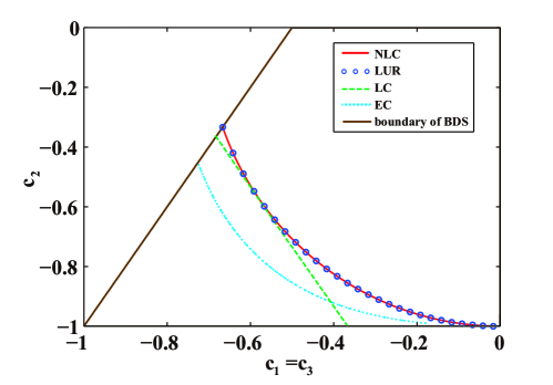
Figure 1: The performances of different quantum steering criteria for the Bell diagonal states under the conditions $c_{1}=c_{3}$. The area inside the brown solid lines denotes Bell diagonal states (BDS). The red solid line, blue circled line, green dashed line, cyan dotted line are given by the nonlinear steering criterion (NLC), local uncertainty relations criterion (LUR), linear criterion (LC), entropic criterion (EC), respectively. States in the left side of these lines are steerable. It is clear that the NLC performs equivalently well as the LUR criterion, which certifies more steerable states than the LC and EC.

(iii) Asymmetric entangled states. Let us consider Gisin states gis , which can be expressed as

$$\rho_{G}=p|\psi_{\theta}\rangle\langle\psi_{\theta}|+(1-p)\rho_{s},$$ (13)

where $\psi_{\theta}=sin\theta|01\rangle+cos\theta|10\rangle$, $\rho_{s}=\frac{1}{2}|00\rangle\langle 00|+\frac{1}{2}|11\rangle\langle 11|$. In Fig.2, we show the performances of the nonlinear steering criterion (Theorem 1), the local uncertainty relations steering criterion zhen , the linear criterion sau and the entropic criterion sch2 for the Gisin states. It follows from straightforward calculation that the nonlinear steering criterion certifies more steerable states than the linear criterion and entropic criterion.

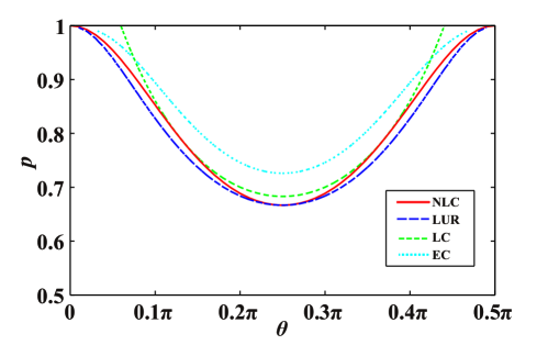
Figure 2: The performances of different quantum steering criteria for the Gisin states. The cyan dotted line, green dashed line, red solid line, blue dashed line are given by the EC, LC, NLC, LUR criterion, respectively. States above these lines are steerable. It is clear that the NLC certifies more steerable states than the LC and EC.

V Conclusion

In summary, we have proposed some nonlinear steering criteria applicable for arbitrary two-qubit quantum systems and optimized ones for symmetric quantum states. These criteria can be used to detect a wide range of steerable quantum states under Pauli measurements. Compared with the existing linear steering criterion and the entropic criterion, ours can certify more steerable states without selecting measurement settings or correlation weights, which can also be used to verify entanglement as all steerable quantum states are entangled.

Appendix A Proof of the equation $\sum_{k=1}^{9}\lambda_{k}=\sum_{i=1}^{3}\sum_{j=1}^{3}\delta^{2}(\sigma_{i}\otimes\sigma_{j})$

In order to prove the Eq. $\sum_{k=1}^{9}\lambda_{k}=\sum_{i=1}^{3}\sum_{j=1}^{3}\delta^{2}(\sigma_{i}\otimes\sigma_{j})$, we extend principal components analysis to quantum correlation matrix $\gamma_{mm^{{}^{\prime}}}(\rho_{AB})$ of local observables $\{O_{m}\}=\{\sigma_{i}\otimes\sigma_{j}\}(i,j=1,2,3,m=3(i-1)+j)$. As in classical correlation analysis, the principal components on a matrix space can be expressed as

$$P_{j}=a_{1j}O_{1}+a_{2j}O_{2}+...+a_{9j}O_{9},$$ (14)

where $j=1,2,...,9$. $\sum_{i}a_{ij}^{*}a_{ij}=1$, and $\sum_{i}a_{ij}^{*}a_{ik}=0$ for $j\neq k$.

To achieve the first principal component, we use the Lagrange multiplier technique to find the maximum of a function. The Lagrangean function is defined as

$$L(a)=tr[\rho(a_{11}O_{1}+a_{21}O_{2}+...+a_{91}O_{9})^{2}]-\{tr[\rho(a_{11}O_{1}+a_{21}O_{2}+...+a_{91}O_{9})]\}^{2}$$

$$+\lambda_{1}(1-a_{11}^{2}-a_{21}^{2}-...-a_{91}^{2}),\ \ \ \ \ \ \ \ \ \ \ \ \ \ \ \ \ \ \ \ \ \ \ \ \ \ \ \ \ \ \ \ \ \ \ \ \ \ \ \ \ \ \ \ \ \ \ \ \ \ \ \ \ \ \ \ \ \ \ \ \ \ \ \ \ \ \ \ \ \ \ \ \ \ \ \ \ \ \$$ (15)

where $\lambda_{1}$ are the Lagrange multipliers. The necessary conditions for the maximum are

$$\frac{\partial L}{\partial a_{11}}=0;\frac{\partial L}{\partial a_{21}}=0;...;\frac{\partial L}{\partial a_{91}}=0.$$ (16)

By using the properties of the trace, we obtain

$$\frac{\partial L}{\partial a_{i1}}=2a_{i1}tr(\rho O_{i}^{2})-2a_{i1}[tr(\rho O_{i})]^{2}+\sum\limits_{k=1,...,9,k\neq i}a_{k1}[tr(\rho O_{i}O_{k})+tr(\rho O_{k}O_{i})]$$

$$-\sum\limits_{k=1,...,9,k\neq i}a_{k1}[tr(\rho O_{i})tr(\rho O_{k})+tr(\rho O_{k})tr(\rho O_{i})]-2\lambda_{1}a_{i1}=0.\ \ \ \ \ \ \ \ \ \ \ \$$ (17)

By rearranging the above expression, we get

$$a_{i1}[tr(\rho O_{i}^{2})-(tr(\rho O_{i}))^{2}]+\{\sum\limits_{k=1,...,9,k\neq i}a_{k1}[tr(\rho O_{i}O_{k})+tr(\rho O_{k}O_{i})]\}/2$$

$$-\sum\limits_{k=1,...,9,k\neq i}a_{k1}tr(\rho O_{i})tr(\rho O_{k})=\lambda_{1}a_{i1}.\ \ \ \ \ \ \ \ \ \ \ \ \ \ \ \ \ \ \ \ \ \ \ \ \ \ \ \ \ \ \ \ \ \ \ \ \ \ \ \ \ \ \ \ \ \ \ \ \ \ \ \ \ \ \ \ \$$ (18)

For $i=1,...,9$, the following eigenvalue problem is obtained in compact form:

$$\gamma\textbf{\emph{a}}_{1}=\lambda_{1}\textbf{\emph{a}}_{1},$$ (19)

where $\textbf{\emph{a}}_{1}=(a_{11},a_{21},...,a_{91})^{\prime}$, $\gamma_{ij}=(\langle O_{i}O_{j}\rangle+\langle O_{j}O_{i}\rangle)/2-\langle O_{i}\rangle\langle O_{j}\rangle$, which is exactly the quantum covariance matrix as defined in Eq.(6). It shows that $\textbf{\emph{a}}_{1}$ should be chosen to be an eigenvector of the covariance matrix $\gamma$, with eigenvalue $\lambda_{1}$. The variance of the first principal component is

$$V(P_{1})=tr(\textbf{\emph{a}}_{1}^{\dagger}\gamma\textbf{\emph{a}}_{1})=\lambda_{1}.$$ (20)

Therefore, in order to obtain the maximum of the variance, $\textbf{\emph{a}}_{1}$ should be chosen as the eigenvector corresponding to the largest eigenvalue $\lambda_{1}$ of the covariance matrix. Similarly, for the second principal component, in order to obtain the second maximum of the variance, $\textbf{\emph{a}}_{2}$ should be chosen as the eigenvector corresponding to the second largest eigenvalue $\lambda_{2}$ of the covariance matrix. This is fully consistent with the classical principal components analysis since the variances correspond to the eigenvalues of the covariance matrix.

For a arbitrary covariance matrix $\gamma_{ij}(\rho_{AB})$ of local observables $\{O_{m}\}=\{\sigma_{i}\otimes\sigma_{j}\}(i,j=1,2,3,m=3(i-1)+j)$, the variance of the observables $O_{m}$ can be analytically given as $\sum_{m=1}^{9}\delta^{2}(O_{m})=\sum_{i=1}^{N}\delta^{2}P_{i}$ due to the fact $\sum_{j}a_{ij}^{*}a_{ij}=1$. As $\sum_{i=1}^{N}\delta^{2}P_{i}=\sum_{i=1}^{N}\lambda_{i}$, one achieves $\sum_{m=1}^{9}\delta^{2}(O_{m})=\sum_{i=1}^{9}\lambda_{i}$.

References

- (1) A. Einstein, B. Podolsky, and N. Rosen, Phys. Rev. 1935, 47, 777.
- (2) E. Schrödinger, Proc. Cambridge Philos. Soc. 1936, 32, 446.
- (3) H. M. Wiseman, S. J. Jones, and A. C. Doherty, Phys. Rev. Lett. 2007, 98, 140402.
- (4) M. D. Reid, Phys. Rev. A 2013, 88, 062338.
- (5) Q. He, L. Rosales-Zrate, G. Adesso, and M. D. Reid, Phys. Rev. Lett. 2015, 115, 180502.
- (6) N. Walk, S. Hosseini, J. Geng, O. Thearle, J. Y. Haw, S. Armstrong, S. M. Assad, J. Janousek, T. C. Ralph, T. Symul, H. M. Wiseman, and P. K. Lam, Optica 2016, 3,634.
- (7) I. Kogias, Y. Xiang, Q. He, and G. Adesso, Phys. Rev. A 2017, 95, 012315.
- (8) C. Branciard, E. G. Cavalcanti, S. P. Walborn, V. Scarani, and H. M. Wiseman, Phys. Rev. A 2012, 85, 010301(R).
- (9) M. Piani and J. Watrous, Phys. Rev. Lett. 2015, 114, 060404.
- (10) R. Horodecki, P. Horodecki, M. Horodecki, and K. Horodecki, Rev. Mod. Phys. 2009, 81, 865.
- (11) J. S. Bell, Physics 1964, 1, 195.
- (12) S. J. Jones, H. M. Wiseman, and A. C. Doherty, Phys. Rev. A 2007, 76, 052116.
- (13) N. Brunner, D. Cavalcanti, S. Pironio, V. Scarant, and S. Wehner, Rev. Mod. Phys. 2014, 86, 419.
- (14) J. Bowles, T. Vértesi, M. T. Quintino, and N. Brunner, Phys. Rev. Lett. 2014, 112, 200402.
- (15) V. Händchen, T. Eberle, S. Steinlechner, A. Samblowski, T. Franz, R. F. Werner, and R. Schnabel, Nature Photonics 2012, 6, 596.
- (16) S. Wollmann, N. Walk, A. J. Bennet, H. M. Wiseman, and G. J. Pryde, Phys. Rev. Lett. 2016, 116, 160403.
- (17) D. J. Saunders, S. J. Jones, H. M. Wiseman, and G. J. Pryde, Nat. Phys. 2010, 6, 845.
- (18) J. Schneeloch, C. J. Broadbent, S. P. Walborn, E. G. Cavalcanti, and J. C. Howell, Phys. Rev. A 2013, 87, 062103.
- (19) S. W. Ji, J. Lee, J. Park, and H. Nha, Phys. Rev. A 2015, 92, 062130.
- (20) Y. Z. Zhen, Y. L. Zheng, W. F. Cao, L. Li, Z. B. Chen, N. L. Liu, and K. Chen, Phys. Rev. A 2016, 93, 012108.
- (21) Y. L. Zheng, Y. Z. Zhen, Z. B. Chen, N. L. Liu, K. Chen, and J. W. Pan, Phys. Rev. A 2017, 95, 012142.
- (22) Y. L. Zheng, Y. Z. Zhen, W. F. Cao, L. Li, Z. B. Chen, N. L. Liu, and K. Chen, Phys. Rev. A 2017, 95, 032128.
- (23) S. X. Yu, Q. Chen, C. J. Zhang, C. H. Lai, and C. H. Oh, Phys. Rev. Lett. 109, 120402 (2012).
- (24) K. Pearson, The London, Edinburgh, and Dublin Philosophical Magazine and Journal of Science 1901, 2, 559.
- (25) H. Hotelling, Journal of Educational Psychology 1933, 24, 417.
- (26) I. T. Jolliffe, Principal Component Analysis, Series: Springer Series in Statistics, 2002, 2nd ed., Springer.
- (27) D. J. Gross, Phys. Today 1995, 48(12), 46 (1995).
- (28) K. G. H. Vollbrecht and R. F. Werner, Phys. Rev. A 2001, 64, 062307.
- (29) J. K. Stockton, J. M. Geremia, A. C. Doherty, and H. Mabuchi, Phys. Rev. A 2003, 67, 022112.
- (30) G. Táth and O. Gühne, Phys. Rev. Lett. 2009, 102, 170503.
- (31) R. F. Werner, Phys. Rev. A 1989, 40, 4277.
- (32) N. Gisin, Phys. Lett. A 1996, 210, 151.