Stage-wise Conservative Linear Bandits

Abstract

We study stage-wise conservative linear stochastic bandits: an instance of bandit optimization, which accounts for (unknown) “safety constraints" that appear in applications such as online advertising and medical trials. At each stage, the learner must choose actions that not only maximize cumulative reward across the entire time horizon, but further satisfy a linear baseline constraint that takes the form of a lower bound on the instantaneous reward. For this problem, we present two novel algorithms, stage-wise conservative linear Thompson Sampling (SCLTS) and stage-wise conservative linear UCB (SCLUCB), that respect the baseline constraints and enjoy probabilistic regret bounds of order $\mathcal{O}(\sqrt{T}\log^{3/2}T)$ and $\mathcal{O}(\sqrt{T}\log T)$, respectively. Notably, the proposed algorithms can be adjusted with only minor modifications to tackle different problem variations, such as, constraints with bandit-feedback, or an unknown sequence of baseline actions. We discuss these and other improvements over the state-of-the art. For instance, compared to existing solutions, we show that SCLTS plays the (non-optimal) baseline action at most $\mathcal{O}(\log{T})$ times (compared to $\mathcal{O}(\sqrt{T})$). Finally, we make connections to another studied form of “safety constraints" that takes the form of an upper bound on the instantaneous reward. While this incurs additional complexity to the learning process as the optimal action is not guaranteed to belong to the “safe set” at each round, we show that SCLUCB can properly adjust in this setting via a simple modification.

1 Introduction

With the growing range of applications of bandit algorithms for safety critical real-world systems, the demand for safe learning is receiving increasing attention Tucker et al., (2020). In this paper, we investigate the effect of stage-wise safety constraints on the linear stochastic bandit problem. Inspired by the earlier work of Kazerouni et al., (2017); Wu et al., (2016), the type of safety constraint we consider in this paper was first introduced by Khezeli and Bitar, (2019). As with the classic linear stochastic bandit problem, the learner wishes to choose a sequence of actions $x_{t}$ that maximize the expected reward over the horizon. However, here the learner is also given a baseline policy that suggests an action with a guaranteed level of expected reward at each stage of the algorithm. This could be based on historical data, e.g., historical ad placement or medical treatment policies with known success rates. The safety constraint imposed on the learner requires her to ensure that the expected reward of her chosen action at every single round be no less than a predetermined fraction of the expected reward of the action suggested by baseline policy. An example that might benefit from the design of stage-wise conservative learning algorithms arises in recommender systems, where the recommender might wish to avoid recommendations that are extremely disliked by the users at any single round. Our proposed stage-wise conservative constraints ensures that at no round would the recommendation system cause severe dissatisfaction for the user, and the reward of action employed by the learning algorithm, if not better, should be close to that of baseline policy. Another example is in clinical trials where the effects of different therapies on patients’ health are initially unknown. We can consider the baseline policy to be treatments that have been historically employed, with known effectiveness. The proposed stage-wise conservative constraint guarantees that at each stage, the learning algorithm suggests an action (a therapy) that achieves the expected reward close to that of the baseline treatment, and as such, this experimentation does not cause harm to any single patient’s health. To tackle this problem, Khezeli and Bitar, (2019) proposed a greedy algorithm called SEGE. They use the decomposition of the regret first proposed in Kazerouni et al., (2017), and show an upper bound of order $\mathcal{O}(\sqrt{T})$ over the number of times that the learning algorithm plays the baseline actions, overall resulting in an expected regret of $\mathcal{O}(\sqrt{T}\log T)$. For this problem, we present two algorithms, SCLTS and SCLUCB, and we provide regret bounds of order $\mathcal{O}(\sqrt{T}\log^{3/2}T)$ and $\mathcal{O}(\sqrt{T}\log T)$, respectively. As it is explained in details in Section 3, we improve the result of Khezeli and Bitar, (2019), i.e., we show our proposed algorithms play the (non-optimal) baseline actions at most $\mathcal{O}(\log{T})$ times, while also relaxing a number of assumptions made in Khezeli and Bitar, (2019). Moreover, we show that our proposed algorithms are adaptable with minor modifications to other safety-constrained variations of this problem. This includes the case where the constraint has a different unknown parameter than the reward function with bandit feedback (Section 3.1), as well as the setting where the reward of baseline action is unknown to the learner in advance (Section 4).

1.1 Conservative Stochastic Linear bandit (LB) Problem with Stage-wise Constraints

Linear Bandit. The learner is given a convex and compact set of actions $\mathcal{X}\subset\mathbb{R}^{d}$. At each round $t$, she chooses an action $x_{t}$ and observes a random reward

$$y_{t}=\langle x_{t},\theta_{\star}\rangle+\xi_{t},$$ (1)

where $\theta_{\star}\in\mathbb{R}^{d}$ is unknown but fixed reward parameter and $\xi_{t}$ is zero-mean additive noise. We let $r_{t}$ be the expected reward of action $x_{t}$ at round $t$, i.e., $r_{t}:=\mathbb{E}[y_{t}]=\langle x_{t},\theta_{\star}\rangle$.

Baseline actions and stage-wise constraint. We assume that the learner is given a baseline policy such that selecting the baseline action $x_{b_{t}}$ at round $t$, she would receive an expected reward $r_{b_{t}}:=\langle x_{b_{t}},\theta_{\star}\rangle$. We assume that the learner knows the expected reward of the actions chosen by the baseline policy. We further assume that the learner’s action selection rule is subject to a stage-wise conservative constraint of the form

$$r_{t}=\langle x_{t},\theta_{\star}\rangle\geq(1-\alpha)r_{b_{t}},$$ (2)

that needs to be satisfied at each round $t$. In particular, constraint (2) guarantees that at each round $t$, the expected reward of the action chosen by the learner stays above the predefined fraction $1-\alpha\in(0,1)$ of the baseline policy. The parameter $\alpha$, controlling the conservatism level of the learning process, is assumed known to the learner similar to Kazerouni et al., (2017); Wu et al., (2016). At each round $t$, an action is called safe if its expected reward is above the predetermined fraction of the baseline policy, i.e., $(1-\alpha)r_{b_{t}}$.

Remark 1.1.

It is reasonable to assume that the leaner has an accurate estimate of the expected reward of the actions chosen by baseline policy Kazerouni et al., (2017). However, in Section 4, we relax this assumption, and propose an algorithm to the case where the expected rewards of the actions chosen by baseline policy are unknown to the learner in advance.

Regret. The cumulative pseudo-regret of the learner up to round $T$ is defined as $R(T)=\sum_{t=1}^{T}\langle x_{\star},\theta_{\star}\rangle-\langle x_{t},\theta_{\star}\rangle$, where $x_{\star}$ is the optimal safe action that maximizes the expected reward,

$$x_{\star}=\arg\max_{x\in\mathcal{X}}\langle x,\theta_{\star}\rangle.$$ (3)

The learner’s objective is to minimize the pseudo-regret, while respecting the stage-wise conservative constraint in (2). For the rest of the paper, we use regret to refer to the pseudo-regret $R(T)$.

1.2 Previous work

Multi-armed Bandits. The multi-armed bandit (MAB) framework has been studied in sequential decision making problems under uncertainty. In particular, it captures the exploration-exploitation trade-off, where the learner needs to sequentially choose arms in order to maximize her reward over time while exploring to improve her estimate of the reward of each arm Bubeck and Eldan, (2016). Two popular heuristics exist for MAB: Following the optimism in face of uncertainty (OFU) principle Auer et al., (2002); Li et al., (2017); Filippi et al., (2010), the so-called Upper Confidence Bound (UCB) based approaches choose the best feasible action- environment pair according to their current confidence regions on the unknown parameter, and Thompson Sampling (TS) Thompson, (1933); Kaufmann et al., (2012); Russo and Van Roy, (2016); Moradipari et al., (2018), which randomly samples the environment and plays the corresponding optimal action.

Linear Stochastic Bandits. There exists a rich literature on linear stochastic bandits. Two well-known efficient algorithms for LB are Linear UCB (LUCB) and Linear Thompson Sampling (LTS). For LUCB, Dani et al., (2008); Rusmevichientong and Tsitsiklis, (2010); Abbasi-Yadkori et al., (2011) provided a regret guarantee of order $\mathcal{O}(\sqrt{T}\log T)$. For LTS, Agrawal and Goyal, (2013); Abeille et al., (2017) provided a regret bound of order $\mathcal{O}(\sqrt{T}\log^{3/2}T)$ in a frequentist setting, i.e., when the unknown parameter $\theta_{\star}$ is a fixed parameter. We need to note that none of the aforementioned heuristics can be directly adopted in the conservative setting. However, note that the regret guarantee provided by our extensions of LUCB and LTS for the safe setting matches those stated for the original setting.

Conservativeness and Safety. The baseline model adopted in this paper was first proposed in Kazerouni et al., (2017); Wu et al., (2016) in the case of cumulative constraints on the reward. In Kazerouni et al., (2017); Wu et al., (2016), an action is considered feasible/safe at round $t$ as long as it keeps the cumulative reward up to round $t$ above a given fraction of a given baseline policy. This differs from our setting, which is focused on stage-wise constraints, where we want the expected reward of the every single action to exceed a given fraction of the baseline reward at each time $t$. This is a tighter constraint than that of Kazerouni et al., (2017); Wu et al., (2016). The setting considered in this paper was first studied in Khezeli and Bitar, (2019), which proposed an algorithm called SEGE to guarantee the satisfaction of the safety constraint at each stage of the algorithm. While our paper is motivated by Khezeli and Bitar, (2019), there are a few key differences: 1) We prove an upper bound of order $\mathcal{O}(\log T)$ for the number of times that the learning algorithm plays the conservative actions which is an order-wise improvement with respect to that of Khezeli and Bitar, (2019), which shows an upper bound of order $\mathcal{O}(\sqrt{T})$; 2) In our setting, the action set is assumed to be a general convex and compact set in $\mathbb{R}^{d}$. However, in Khezeli and Bitar, (2019), the proof relies on the action set being a specific ellipsoid; 3) In Section 4, we provide a regret guarantee for the learning algorithm for the case where the baseline reward is unknown. However, the results of Khezeli and Bitar, (2019) have not been extended to this case; 4) In Section 3.1, we also modify our proposed algorithm and provide a regret guarantee for the case where the constraint has a different unknown parameter than the one in the reward function. However, this is not discussed in Khezeli and Bitar, (2019). Another difference between the two works is on the type of performance guarantees. In Khezeli and Bitar, (2019), the authors bound the expected regret. Towards this goal, they manage to quantify the effect of the risk level $\delta$ on the regret and constraint satisfaction. However, it appears that the analysis in Khezeli and Bitar, (2019) is limited to ellipsoidal action sets. Instead, in this paper, we present a bound on the regret that holds with high (constant) probability (parameterized by $\delta$) over all $T$ rounds of the algorithm. This type of results is very common in the bandit literature, e.g. Abbasi-Yadkori et al., (2011); Dani et al., (2008), and in the emerging safe-bandit literature Kazerouni et al., (2017); Amani et al., (2019); Sui et al., (2018).

Another variant of safety w.r.t a baseline policy has also been studied in Mansour et al., (2015); Katariya et al., (2018) in the multi-armed bandits framework. Moreover, there has been an increasing attention on studying the effect of safety constraints in the Gaussian process (GP) optimization literature. For example, Sui et al., (2015, 2018) study the problem of nonlinear bandit optimization with nonlinear constraints using GPs (as non-parametric models). The algorithms in Sui et al., (2015, 2018) come with convergence guarantees but no regret bound. Moreover, Ostafew et al., (2016); Akametalu et al., (2014) study safety-constrained optimization using GPs in robotics applications. A large body of work has considered safety in the context of model-predictive control, see, e.g., Aswani et al., (2013); Koller et al., (2018) and references therein. Focusing specifically on linear stochastic bandits, extension of UCB-type algorithms to provide safety guarantees with provable regret bounds was considered recently in Amani et al., (2019). This work considers the effect of a linear constraint of the form $x^{\top}B\theta_{\star}\leq C,$ where $B$ and $C$ are respectively a known matrix and positive constant, and provides a problem dependent regret bound for a safety-constrained version of LUCB that depends on the location of the optimal action in the safe action set. Notice that this setting requires the linear function $x^{\top}B\theta_{\star}$ to remain below a threshold $C$, as opposed to our setting which considers a lower bound on the reward. We note that the algorithm and proof technique in Amani et al., (2019) does not extend to our setting and would only work for inequalities of the given form; however, we discuss how our algorithm can be modified to provide a regret bound of order $\mathcal{O}(\sqrt{T}\log T)$ for the setting of Amani et al., (2019) in Appendix H. A TS variaent of this setting has been studied in Moradipari et al., (2020, 2019)

1.3 Model Assumptions

Notation. The weighted $\ell_{2}$-norm with respect to a positive semi-definite matrix $V$ is denoted by $\|x\|_{V}=\sqrt{x^{\top}Vx}$. The minimum of two numbers $a,b$ is denoted $a\wedge b$. Let $\mathcal{F}_{t}=(\mathcal{F}_{1},\sigma(x_{1},\xi_{1},\dots,x_{t},\xi_{t}))$ be the filtration ($\sigma$-algebra) that represents the information up to round $t$.

Assumption 1.

For all $t$, $\xi_{t}$ is conditionally zero-mean R-sub-Gaussian noise variables, i.e., $\mathbb{E}[\xi_{t}|\mathcal{F}_{t-1}]=0$, and $\mathbb{E}[e^{\lambda\xi_{t}}|\mathcal{F}_{t-1}]\leq\exp{(\frac{\lambda^{2}R^{2}}{2})},\forall\lambda\in\mathbb{R}^{d}$.

Assumption 2.

There exists a positive constant $S$ such that $\|\theta_{\star}\|_{2}\leq S$.

Assumption 3.

The action set $\mathcal{X}$ is a compact and convex subset of $\mathbb{R}^{d}$ that contains the unit ball. We assume that $\|x\|_{2}\leq L,\forall x\in\mathcal{X}$. Also, we assume $\langle x,\theta_{\star}\rangle\leq 1,\forall x\in\mathcal{X}$.

Let $\kappa_{b_{t}}=\langle x_{\star},\theta_{\star}\rangle-r_{b_{t}}$ be the difference between expected reward of the optimal and baseline actions at round $t$. As in Kazerouni et al., (2017), we assume the following.

Assumption 4.

There exist $0\leq\kappa_{l}\leq\kappa_{h}$ and $0<r_{l}\leq r_{h}$ such that, at each round $t$

$$\kappa_{l}\leq\kappa_{b_{t}}\leq\kappa_{h}\leavevmode\nobreak\ \text{and}\leavevmode\nobreak\ r_{l}\leq r_{b_{t}}\leq r_{h}.$$ (4)

We note that since these parameters are associated with the baseline policy, it can be reasonably assumed that they can be estimated accurately from data. This is because we think of the baseline policy as “past strategy”, implemented before bandit-optimization, thus producing large amount of data. The lower bound $0<r_{l}\leq r_{b_{t}}$ on the baseline reward ensures a minimum level of performance at each round. $\kappa_{h}$ and $r_{h}$ could be at most 1, due to Assumption 3. For simplicity, we assume the lower bound $\kappa_{l}$ on the sub-optimality gap $\kappa_{b_{t}}$ is known. If not, we can always choose $\kappa_{l}=0$ by optimality of $x_{\star}$.

2 Stage-wise Conservative Linear Thompson Sampling (SCLTS) Algorithm

In this section we propose a TS variant algorithm in a frequentist setting referred to as Stage-wise Conservative Linear Thompson Sampling (SCLTS) for the problem setting in Section 1.1. Our adoption of TS is due to its well-known computational efficiency over UCB-based algorithms, since action selection via the latter involves solving optimization problems with bilinear objective functions, whereas the former would lead to linear objectives. However, this choice does not fundamentally affect our approach. In fact, in Appendix G, we propose a Stage-wise Conservative Linear UCB (SCLUCB) algorithm, and we provide the regret guarantee for it. In particular, we show a regret of order $\mathcal{O}\left(d\sqrt{T}\log(\frac{TL^{2}}{\lambda\delta})\right)$ for SCLUCB, which has the same order as the lower bound proposed for LB in Dani et al., (2008); Rusmevichientong and Tsitsiklis, (2010).

At each round $t$, given a regularized least-square (RLS) estimate of $\hat{\theta}_{t}$, SCLTS samples a perturbed parameter $\tilde{\theta}_{t}$ with an appropriate distributional property. Then, it searches for the action that maximizes the expected reward considering the parameter $\tilde{\theta}_{t}$ as the true parameter while respecting the safety constraint (2). If any such action exists, it is played under certain conditions; else, the algorithm resorts to playing a perturbed version of the baseline action that satisfies the safety constraint. In order to guarantee constraint satisfaction (a.k.a safety of actions), the algorithm builds a confidence region $\mathcal{E}_{t}$ that contains the unknown parameter $\theta_{\star}$ with high probability. Then, it constructs an estimated safe set $\mathcal{X}_{t}^{s}$ such that all actions $x_{t}\in\mathcal{X}_{t}^{s}$ satisfy the safety constraint for all $v\in\mathcal{E}_{t}$. The summary of the SCLTS presented in Algorithm 1, and a detailed explanation follows.

1

2

3Input: $\delta,T,\lambda,\rho_{1}$

4Set $\delta^{\prime}=\frac{\delta}{4T}$

5 for $t=1,\dots,T$  do

6       Sample $\eta_{t}\sim\mathcal{H}^{\text{TS}}$

7      

8      Compute RLS-estimate $\hat{\theta}_{t}$ and $V_{t}$ according to (5)

9      Set $\tilde{\theta}_{t}=\hat{\theta}_{t}+\beta_{t}V_{t}^{-1/2}\eta_{t}$

10      

11      Build the confidence region $\mathcal{E}_{t}(\delta^{\prime})$ in (6)

12      Compute the estimated safe set $\mathcal{X}_{t}^{s}$ in (8)

13      

14      if the following optimization is feasible: $x(\tilde{\theta}_{t})=\text{argmax}_{x\in\mathcal{X}_{t}^{s}}\langle x,\tilde{\theta}_{t}\rangle$, then

15      Set $F=1$, else $F=0$

16      

17      if $F=1$ and $\lambda_{\text{min}}(V_{t})\geq\left(\frac{2L\beta_{t}}{\kappa_{l}+\alpha r_{b_{l}}}\right)^{2}$, then

18      Play $x_{t}=x(\tilde{\theta}_{t})$

19      else

20      Play $x_{t}=(1-\rho_{1})x_{b_{t}}+\rho_{1}\zeta_{t}$

21      Observe reward $y_{t}$ in (1)

22      

end for

Algorithm 1 Stage-wise Conservative Linear Thompson Sampling (SCLTS)

2.1 Algorithm description

Let $x_{1},\dots,x_{t}$ be the sequence of the actions and $r_{1},\dots,r_{t}$ be their corresponding rewards. For any $\lambda>0$, we can obtain a regularized least-squares (RLS) estimate $\hat{\theta}_{t}$ of $\theta_{\star}$ as follows

$$\hat{\theta}_{t}=V_{t}^{-1}\sum_{s=1}^{t-1}y_{s}x_{s},\leavevmode\nobreak\ \text{where}\leavevmode\nobreak\ V_{t}=\lambda I+\sum_{s=1}^{t-1}x_{s}x_{s}^{\top}.$$ (5)

Algorithm 1 construct a confidence region

$$\mathcal{E}_{t}(\delta^{\prime})=\mathcal{E}_{t}:=\{\theta\in\mathbb{R}^{d}:\|\theta-\hat{\theta}_{t}\|_{V_{t}}\leq\beta_{t}(\delta^{\prime})\},$$ (6)

where the ellipsoid radius $\beta_{t}$ is chosen according to the Proposition 2.1 in Abbasi-Yadkori et al., (2011) (restated below for completeness) in order to guarantee that $\theta_{\star}\in\mathcal{E}_{t}$ with high probability.

Proposition 2.1.

( Abbasi-Yadkori et al., (2011)) Let Assumptions 1, 2, and 3 hold. For a fixed $\delta\in(0,1)$, and

$$\beta_{t}(\delta)=R\sqrt{d\log\left(\frac{1+\frac{tL^{2}}{\lambda}}{\delta}\right)}+\sqrt{\lambda}S$$ (7)

with probability at least $1-\delta$, it holds that $\theta_{\star}\in\mathcal{E}_{t}$.

2.1.1 The estimated safe action set

Since $\theta_{\star}$ is unknown to the learner, she does not know whether an action $x\in\mathcal{X}$ is safe or not. Thus, she builds an estimated safe set such that each action $x_{t}\in\mathcal{X}_{t}^{s}$ satisfies the safety constraint for all $v\in\mathcal{E}_{t}$, i.e.,

$$\mathcal{X}_{t}^{s}:= \{x\in\mathcal{X}:\langle x,v\rangle\geq(1-\alpha)r_{b_{t}},\forall v\in\mathcal{E}_{t}\}=\{x\in\mathcal{X}:\min_{v\in\mathcal{E}_{t}}\langle x,v\rangle\geq(1-\alpha)r_{b_{t}}\}$$ (8)

$$=\{x\in\mathcal{X}:\langle x,\hat{\theta}_{t}\rangle-\beta_{t}(\delta^{\prime})\|x\|_{V_{t}^{-1}}\geq(1-\alpha)r_{b_{t}}\}.$$ (9)

Note that $\mathcal{X}_{t}^{s}$ is easy to compute since (9) involves a convex quadratic program. In order to guarantee safety, at each round $t$, the learner chooses her actions only from this estimated safe set in order to maximize the reward given the sampled parameter $\tilde{\theta}_{t}$, i.e.,

$$x(\tilde{\theta}_{t})=\arg\max_{x\in\mathcal{X}_{t}^{s}}\langle x,\tilde{\theta}_{t}\rangle,$$ (10)

where $\tilde{\theta}_{t}=\hat{\theta}_{t}+\beta_{t}V_{t}^{-1/2}\eta_{t}$, and $\eta_{t}$ is a random IID sample from a distribution $\mathcal{H}^{\text{TS}}$ that satisfies certain distributional properties (see Abeille et al., (2017) or Defn. C.1 in Appendix C for more details). The challenge with $\mathcal{X}_{t}^{s}$ is that it contains actions which are safe with respect to all the parameters in $\mathcal{E}_{t}$, and not only $\theta_{\star}$. Hence, there may exist some rounds that $\mathcal{X}_{t}^{s}$ is empty. In order to face this problem, the algorithm proceed as follows. At round $t$, if the estimated action set $\mathcal{X}_{t}^{s}$ is not empty, SCLTS plays the safe action $x(\tilde{\theta}_{t})$ in (10) only if the minimum eigenvalue of the Gram matrix $V_{t}$ is greater than $k_{t}^{1}=\left(\frac{2L\beta_{t}}{\kappa_{l}+\alpha r_{b_{l}}}\right)^{2}$, i.e., $\lambda_{\text{min}}(v_{t})\geq k_{t}^{1}$, where $k_{t}^{1}$ is of order $\mathcal{O}(\log t)$. Otherwise, it plays the conservative action which is presented next. We show in Appendix C that $\lambda_{\text{min}}(v_{t})\geq k_{t}^{1}$ ensures that for the rounds that SCLTS plays the action $x(\tilde{\theta}_{t})$ in (10), the optimal action $x_{\star}$ belongs to the estimated safe set $\mathcal{X}_{t}^{s}$, from which we can bound the regret of Term I in (12).

2.1.2 Conservative actions

In our setting, we assume that the learner is given a baseline policy that at each round $t$ suggests a baseline action $x_{b_{t}}$. We employ the idea proposed in Khezeli and Bitar, (2019), which is merging the baseline actions with random exploration actions under stage-wise safety constraint. In particular, at each round $t$, SCLTS constructs a conservative action $x_{t}^{\text{cb}}$ as a convex combination of the baseline action $x_{b_{t}}$ and a random vector $\zeta_{t}$ as follows:

$$x_{t}^{\text{cb}}=(1-\rho_{1})x_{b_{t}}+\rho_{1}\zeta_{t},$$ (11)

where $\zeta_{t}$ is assumed to be a sequence of independent, zero-mean and bounded random vectors. Moreover, we assume that $\|\zeta_{t}\|_{2}=1$ almost surely and $\sigma^{2}_{\zeta}=\lambda_{\text{min}}(\text{Cov}(\zeta_{t}))>0$. The parameters $\sigma_{\zeta}$ and $\rho_{1}$ control the exploration level of the conservative actions. In order to ensure that the conservative actions are safe, in Lemma 2.2, we establish an upper bound on $\rho_{1}$ such that for all $\rho_{1}\in(0,\bar{\rho})$, the conservative action $x_{t}^{\text{cb}}=(1-\rho_{1})x_{b_{t}}+\rho_{1}\zeta_{t}$ is guaranteed to be safe.

Lemma 2.2.

At each round $t$, given the fraction $\alpha$, for any $\rho\in(0,\bar{\rho})$, where $\bar{\rho}=\frac{\alpha r_{l}}{S+r_{h}}$, the conservative action $x_{t}^{\text{cb}}=(1-\rho)x_{b_{t}}+\rho\zeta_{t}$ is guaranteed to be safe almost surely.

For the ease of notation, in the rest of this paper, we simply assume that $\rho_{1}=\frac{r_{l}}{S+r_{h}}\alpha$.

At round $t$, SCLTS plays the conservative action $x_{t}^{\text{cb}}$ if the two conditions defined in Section 2.1.1 do not hold, i.e., either the estimated safe set $\mathcal{X}_{t}^{s}$ is empty or $\lambda_{\text{min}}(V_{t})<k_{t}^{1}$.

3 Regret Analysis

In this section, we provide a tight regret bound for SCLTS. In Proposition 3.1, we show that the regret of SCLTS can be decomposed into regret caused by choosing safe Thompson Sampling actions plus that of playing conservative actions. Then, we bound both terms separately. Let $N_{t-1}$ be the set of rounds $i<t$ at which SCLTS plays the action in (10). Similarly, $N_{t-1}^{c}=\{1,\dots,t-1\}-N_{t-1}$ is the set of rounds $j<t$ at which SCLTS plays the conservative actions.

Proposition 3.1.

The regret of SCLTS can be decomposed into two terms as follows:

$$R(T)\leq\underbrace{\sum_{t\in N_{T}}\left(\langle x_{\star},\theta_{\star}\rangle-\langle x_{t},\theta_{\star}\rangle\right)}_{\text{Term I}}+\underbrace{|N_{T}^{{c}}|\left(\kappa_{h}+\rho_{1}(r_{h}+S)\right)}_{\text{Term II}}$$ (12)

The idea of bounding Term I is inspired by Abeille et al., (2017): we wish to show that LTS has a constant probability of being "optimistic", in spite of the need to be conservative. In Theorem 3.2, we provide an upper bound on the regret of Term I which is of order $\mathcal{O}(d^{3/2}\log^{1/2}d\leavevmode\nobreak\ T^{1/2}\log^{3/2}T)$.

Theorem 3.2.

Let $\lambda,L\geq 1$. On event $\{\theta_{\star}\in\mathcal{E}_{t},\forall t\in[T]\}$, and under Assumption 4, we can bound Term I in (12) as:

Term I $$\leq(\beta_{T}(\delta^{\prime})+\gamma_{T}(\delta^{\prime})(1+\frac{4}{p}))\sqrt{2Td\log{(1+\frac{TL^{2}}{\lambda})}}+\frac{4\gamma_{T}(\delta^{\prime})}{p}\sqrt{\frac{8TL^{2}}{\lambda}\log{\frac{4}{\delta}}},$$ (13)

where $\delta^{\prime}=\frac{\delta}{6T}$, and $\gamma_{t}(\delta)=\beta_{t}(\delta^{\prime})\left(1+\frac{2}{C}\right)\sqrt{cd\log{(\frac{c^{\prime}d}{\delta})}}$

We note that the regret of Term I has the same bound as that of Abeille et al., (2017) in spite of the additional safety constraints imposed on the problem. As the next step, in order to bound Term II in (12), we need to find an upper bound on the number of times $|N_{T}^{c}|$ that SCLTS plays the conservative actions up to time $T$. We prove an upper bound on $|N_{T}^{c}|$ in Theorem 3.3.

Theorem 3.3.

Let $\lambda,L\geq 1$. On event $\{\theta_{\star}\in\mathcal{E}_{t},\forall t\in[T]\}$, and under Assumption 4, it holds that

$$|N_{T}^{c}|\leq\left(\frac{2L\beta_{T}}{\rho_{1}\sigma_{\zeta}(\kappa_{l}+\alpha r_{l})}\right)^{2}+\frac{2h_{1}^{2}}{\rho_{1}^{4}\sigma_{\zeta}^{4}}\log(\frac{d}{\delta})+\frac{2Lh_{1}\beta_{T}\sqrt{8\log(\frac{d}{\delta})}}{\rho_{1}^{3}\sigma_{\zeta}^{3}(\kappa_{l}+\alpha r_{l})},$$ (14)

where $h_{1}=2\rho_{1}(1-\rho_{1})L+2\rho_{1}^{2}$ and $\rho_{1}=(\frac{r_{l}}{S+r_{h}})\alpha$.

Remark 3.1.

The upper bound on the number of times SCLTS plays the conservative actions up to time T provided in Theorem 3.3 has the order $\mathcal{O}\left(\frac{L^{2}d\log(\frac{T}{\delta})\log(\frac{d}{\delta})}{\alpha^{4}(r_{l}^{2}\wedge r_{l}^{4})\kappa_{l}(\sigma_{\zeta}^{2}\wedge\sigma_{\zeta}^{4})}\right)$.

The first idea of the proof is based on the intuition that if a baseline action is played at round $\tau$, then the algorithm does not yet have a good estimate of the unknown parameter $\theta_{\star}$ and the safe actions played thus far have not yet expanded properly in all directions. Formally, this translates to small $\lambda_{\text{min}}(V_{\tau})$ and the upper bound $O(\log\tau)\geq\lambda_{\text{min}}(V_{\tau})$. The second key idea is to exploit the randomized nature of the conservative actions (cf. (11)) to lower bound $\lambda_{\text{min}}(V_{\tau})$ by the number of times ($N_{\tau}^{c}$) that SCLTS plays the baseline actions up to that round (cf. Lemma D.1 in the Appendix). Putting these together leads to the advertised upper bound $O(\log T)$ on the total number of times ($N_{T}^{c}$) the algorithm plays the baseline actions.

3.1 Additional Side Constraint with Bandit Feedback

We also consider the setting where the constraint depends on an unknown parameter that is different than the one in reward function. In particular, we assume the constraint of the form

$$\langle x_{t},\mu_{\star}\rangle\geq(1-\alpha)q_{b_{t}},$$ (15)

which needs to be satisfied by the action $x_{t}$ at every round $t$. In (15), $\mu_{\star}$ is a fixed, but unknown and the positive constants $q_{b_{t}}=\langle x_{b_{t}},\mu_{\star}\rangle$ are known to the learner. In Section 4, we relax this assumption and we consider the case where the learner does not know the value of $q_{b_{t}}$. Let $\nu_{b_{t}}=\langle x_{\star},\mu_{\star}\rangle-\langle x_{b_{t}},\mu_{\star}\rangle$. Similar to Assumption 4, we assume there exist constants $0\leq\nu_{l}\leq\nu_{h}$ and $0<r_{l}\leq r_{h}$ such that $\nu_{l}\leq\nu_{b_{t}}\leq\nu_{h}$ and $r_{l}\leq r_{b_{t}}\leq r_{h}$.

We assume that with playing an action $x_{t}$, the learner observes the following bandit feedback:

$$w_{t}=\langle x_{t},\mu_{\star}\rangle+\chi_{t},$$ (16)

where $\chi_{t}$ is assumed to be a zero-mean $R$-sub-Gaussian noise. In order to handle this case, we show how SCLTS should be modified, and we propose a new algorithm called SCLTS-BF. The details on SCLTS-BF are presented in Appendix E. In the following, we only mention the difference of SCLTS-BF with SCLTS, and show an upper bound on its regret.

The main difference is that SCLTS-BF constructs two confidence regions $\mathcal{E}_{t}$ in (6) and $\mathcal{C}_{t}$ based on the bandit feedback such that $\theta_{\star}\in\mathcal{E}_{t}$ and $\mu_{\star}\in\mathcal{C}_{t}$ with high probability. Then, based on $\mathcal{C}_{t}$, it constructs the estimated safe decision set denoted $\mathcal{P}_{t}^{s}=\{x\in\mathcal{X}:\langle x,v\rangle\geq(1-\alpha)q_{b_{t}},\forall v\in\mathcal{C}_{t}\}$. We note that SCLTS-BF only plays the actions from $\mathcal{P}_{t}^{s}$ that are safe with respect to all the parameters in $\mathcal{C}_{t}$.

We report the details on proving the regret bound for SCLTS-BF in Appendix E. We use the decomposition in Proposition 3.1, and we upper bound Term I similar to the Theorem 3.2. Then, we show an upper bound of order $\mathcal{O}\left(\frac{L^{2}d\log(\frac{T}{\delta})\log(\frac{d}{\delta})}{\alpha^{4}(q_{l}^{2}\wedge q_{l}^{4})\kappa_{l}(\sigma_{\zeta}^{2}\wedge\sigma_{\zeta}^{4})}\right)$ over the number of times that SCLTS-BF plays the conservative actions.

4 Unknown Baseline Reward

Inspired by Kazerouni et al., (2017), which studies this problem in the presence of safety constraints on the cumulative rewards, we consider the case where the expected reward of the action chosen by baseline policy, i.e., $r_{b_{t}}$ is unknown to the learner. However, we assume that the learner knows the value of $r_{l}$ in (4). We describe the required modifications on SCLTS to handle this case, and present a new algorithm called SCLTS2. Then, we prove the regret bound for SCLTS2, which has the same order as SCLTS.

Here, the learner does not know the value of $r_{b_{t}}$; however, she knows that the unknown parameter $\theta_{\star}$ falls in the confidence region $\mathcal{E}_{t}$ with high probability. Hence, we can upper bound the RHS of (2) with $\max_{v\in\mathcal{E}_{t}}\langle x_{b_{t}},v\rangle\geq r_{b_{t}}$. Therefore, any action $x$ that satisfies

$$\min_{v\in\mathcal{E}_{t}}\langle x(\tilde{\theta}_{t}),v\rangle\geq(1-\alpha)\max_{v\in\mathcal{E}_{t}}\langle x_{b_{t}},v\rangle,$$ (17)

is safe with high probability. In order to ensure safety, SCLTS2 only plays the safe actions from the estimated safe actions set $\mathcal{Z}_{t}^{s}=\{x\in\mathcal{X}:\min_{v\in\mathcal{E}_{t}}\langle x,v\rangle\geq(1-\alpha)\max_{v\in\mathcal{E}_{t}}\langle x_{b_{t}},v\rangle\}$. We report the details on SCLTS2 in Appendix F.

Next, we provide an upper bound on the regret of SCLTS2. To do so, we first use the decomposition in Proposition 3.1. The regret of Term I is similar to that of SCLTS (Theorem 3.2), and in Theorem 4.1, we prove an upper bound on the number of time SCLTS2 plays the conservative actions. Note that similar steps can be generalized to the setting of additional side constraints with bandit feedback.

Theorem 4.1.

Let $\lambda,L\geq 1$. On event $\{\theta_{\star}\in\mathcal{E}_{t},\forall t\in[T]\}$, and under Assumption 4, we can upper bound the number of times SCLTS2 plays the conservative actions, i.e., $|N_{T}^{c}|$ as:

$$|N_{T}^{c}|\leq\left(\frac{2L\beta_{T}(2-\alpha)}{\rho_{3}\sigma_{\zeta}(\kappa_{l}+\alpha r_{l})}\right)^{2}+\frac{2h_{3}^{2}}{\rho_{3}^{4}\sigma_{\zeta}^{4}}\log(\frac{d}{\delta})+\frac{2Lh_{3}\beta_{T}(2-\alpha)}{\rho_{3}^{3}\sigma_{\zeta}^{3}(\kappa_{l}+\alpha r_{l})}\sqrt{8\log(\frac{d}{\delta})},$$ (18)

where $h_{3}=2\rho_{3}(1-\rho_{3})L+2\rho_{3}^{2}$ and $\rho_{3}=(\frac{r_{l}}{S+1})\alpha$.

Remark 4.1.

The regret of SCLTS2 has order of $\mathcal{O}\left(\frac{L^{2}d\log(\frac{T}{\delta})\log(\frac{d}{\delta})(2-\alpha)^{2}}{\alpha^{4}(r_{l}^{2}\wedge r_{l}^{4})\kappa_{l}(\sigma_{\zeta}^{2}\wedge\sigma_{\zeta}^{4})}\right)$, which has the same rate as that of SCLTS. Therefore, the lack of information about the reward function only hurt the regret with a constant $(2-\alpha)^{2}$.

5 Numerical Results

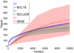
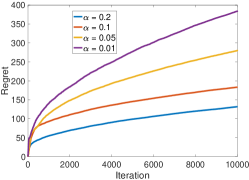
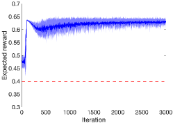
Figure 1: Left: comparison of the cumulative regret of SCLTS and SCLUCB versus SEGE algorithm in Khezeli and Bitar, (2019). Middle: average regret (over 100 runs) of SCLTS algorithm for different values of $\alpha$. Right: expected reward under SCLTS algorithm in the first $3000$ rounds for $\alpha=0.2$.

In this section, we investigate the numerical performance of SCLTS and SCLUCB on synthetic data, and compare it with SEGE algorithm introduced by Khezeli and Bitar, (2019). In all the implementations, we used the following parameters: $R=0.1,S=1,\lambda=1,d=2$. We consider the action set $\mathcal{X}$ to be a unit ball centered on the origin. The reward parameter $\theta_{\star}$ is drawn from $\mathcal{N}(0,I_{4})$. We generate the sequence $\{\zeta_{t}\}_{t=1}^{\infty}$ to be IID random vectors that are uniformly distributed on the unit circle. The results are averaged over 100 realizations.

In Figure 1(left), we plot the cumulative regret of the SCLTS algorithm and SCLUCB and SEGE algorithm from Khezeli and Bitar, (2019) for $\alpha=0.2$ over $100$ realizations. The shaded regions show standard deviation around the mean. In view of the discussion in Dani et al., (2008) regarding computational issues of LUCB algorithms with confidence regions specified with $\ell_{2}$-norms, we implement a modified version of Safe-LUCB which uses $\ell_{1}$-norms instead of $\ell_{2}$-norms. Figure 1(left) shows that SEGE algorithm suffers a high variance of the regret over different problem instances which shows the strong dependency of the performance of SEGE algorithm on the specific problem instance. However, the regret of SCLTS and SCLUCB algorithms do not vary significantly under different problem instances, and has a low variance. Moreover, the regret of SEGE algorithm grows faster in the beginning steps, since it heavily relies on the baseline action in order to satisfy the safety constraint. However, the randomized nature of SCLTS leads to a natural exploration ability that is much faster in expanding the estimated safe set, and hence it plays the baseline actions less frequently than SEGE algorithm even in the initial exploration stages.

In Figure 1(middle), we plot the average regret of SCLTS for different values of $\alpha$ over a horizon $T=10000$. Figure 1(middle) shows that, SCLTS has a better performance (i.e., smaller regret) for the larger value of $\alpha$, since for the small value of $\alpha$, SCLTS needs to be more conservative in order to satisfy the safety constraint, and hence it plays more baseline actions. Moreover, Figure 1(right) illustrates the expected reward of SCLTS algorithm in the first $3000$ rounds. In this setting, we assume there exists one baseline action $x_{b}=[0.6,0.5]$, which is available to the learner, $\theta_{\star}=[0.5,0.4]$ and the safety fraction $\alpha=0.2$. Thus, the safety threshold is $(1-\alpha)\langle x_{b},\theta_{\star}\rangle=0.4$ (shown as a dashed red line), which SCLTS respects in all rounds. In particular, in initial rounds, SCTLS plays the conservative actions in order to respect the safety constraint, which as shown have an expected reward close to 0.475. Over time as the algorithm achieves a better estimate of the unknown parameter $\theta_{\star}$, it is able to play more optimistic actions and as such receives higher rewards.

6 Conclusion

In this paper, we study the stage-wise conservative linear stochastic bandit problem. Specifically, we consider safety constraints that requires the action chosen by the learner at each individual stage to have an expected reward higher than a predefined fraction of the reward of a given baseline policy. We propose extensions of Linear Thompson Sampling and Linear UCB in order to minimize the regret of the learner while respecting safety constraint with high probability and provide regret guarantees for them. We also consider the setting of constraints with bandit feedback, where the safety constraint has a different unknown parameter than that of the reward function, and we propose the SCLTS-BF algorithm to handle this case. Third, we study the case where the rewards of the baseline actions are unknown to the learner. Lastly, our numerical experiments compare the performance of our algorithm to SEGE of Khezeli and Bitar, (2019) and showcase the value of the randomized nature of our exploration phase. In particular, we show that the randomized nature of SCLTS leads to a natural exploration ability that is faster in expanding the estimated safe set, and hence SCLTS plays the baseline actions less frequently as theoretically shown. For future work, natural extension of the problem setting to generalized linear bandits, and possibly with generalized linear constrains might be of interest.

7 Acknowledgment

This research is supported by NSF grant 1847096. C. Thrampoulidis was partially supported by the NSF under Grant Number 1934641.

8 Broader Impact

The main goal of this paper is to design and study novel “safe” learning algorithms for safety-critical systems with provable performance guarantees. An example arises in clinical trials where the effect of different therapies on patient’s health is not known in advance. We select the baseline actions to be the therapies that have been historically chosen by medical practitioners, and the reward captures the effectiveness of the chosen therapy. The stage-wise conservative constraint modeled in this paper ensures that at each round the learner should choose a therapy which results in an expected reward if not better, must be close to the baseline policy. Another example arises in societal-scale infrastructure networks such as communication/power/transportation/data network infrastructure. We focus on the case where the reliability requirements of network operation at each round depends on the reward of the selected action and certain baseline actions are known to not violate system constraints and achieve certain levels of operational efficiency as they have been used widely in the past. In this case, the stage-wise conservative constraint modeled in this paper ensures that at each round, the reward of action employed by learning algorithm if not better, should be close to that of baseline policy in terms of network efficiency, and the reliability requirement for network operation must not be violated by the learner. Another example is in recommender systems that at each round, we wish to avoid recommendations that are extremely disliked by the users. Our proposed stage-wise conservative constrains ensures that at no round would the recommendation system cause severe dissatisfaction for the users (consider perhaps how a really bad personal movie recommendation from a streaming platform would severely affect your view of the said platform).

Appendix A Proof of Proposition 3.1

From the definition of regret, we can write

$$R(T) =\sum_{t\in N_{T}}\left(\langle x_{\star},\theta_{\star}\rangle-\langle x_{t},\theta_{\star}\rangle\right)+\sum_{t\in N_{T}^{c}}\left(\langle x_{\star},\theta_{\star}\rangle-\langle(1-\rho_{1})x_{b_{t}}-\rho_{1}\zeta_{t},\theta_{\star}\rangle\right)$$

$$=\sum_{t\in N_{T}}\left(\langle x_{\star},\theta_{\star}\rangle-\langle x_{t},\theta_{\star}\rangle\right)+\sum_{t\in N_{T}^{c}}\bigg{(}\langle x_{\star},\theta_{\star}\rangle-\langle x_{b_{t}},\theta_{\star}\rangle+\rho_{1}\langle x_{b_{t}},\theta_{\star}\rangle+\rho_{1}\langle\zeta_{t},\theta_{\star}\rangle\bigg{)}$$

$$\leq\sum_{t\in N_{T}}\left(\langle x_{\star},\theta_{\star}\rangle-\langle x_{t},\theta_{\star}\rangle\right)+|N_{T}^{c}|\left(\kappa_{h}+\rho_{1}(r_{h}+S)\right).$$ (19)

Appendix B Proof of Lemma 2.2

In order to ensure that the conservative action $x_{t}=(1-\rho)x_{b_{t}}-\rho\zeta_{t}$ is safe, we need to show that it satisfies (2). Hence, it suffices to show that

$$\langle(1-\rho)x_{b_{t}}-\rho\zeta_{t},\theta_{\star}\rangle\geq(1-\alpha)r_{b_{t}}.$$ (20)

We can lower bound the LHS of (20) as follows:

$$\langle(1-\rho)x_{b_{t}}-\rho\zeta_{t},\theta_{\star}\rangle=r_{b_{t}}-\rho r_{b_{t}}-\rho\langle\zeta_{t},\theta_{\star}\rangle\geq r_{b_{t}}-\rho r_{b_{t}}-\rho S.$$

Recall that $\|\zeta_{t}\|_{2}=1$ almost surely, and due to Assumption 2, we know that $\|\theta_{\star}\|_{2}\leq S$. Hence, it suffices to show that

$$r_{b_{t}}-\rho r_{b_{t}}-\rho S\geq(1-\alpha)r_{b_{t}},$$

or equivalently,

$$\rho r_{b_{t}}+\rho S\leq\alpha r_{b_{t}}$$ (21)

From (21) we can write

$$\rho\leq\frac{\alpha r_{b_{t}}}{S+r_{b_{t}}}.$$ (22)

Therefore, for any $\rho$ satisfying (22), the conservative action $x_{t}=(1-\rho)x_{b_{t}}+\rho\zeta_{t}$ is guaranteed to be safe almost surely. Then, we lower bound the right hand side of (22) using Assumption 4, and we establish the following upper bound on $\rho$,

$$\rho\leq\frac{\alpha r_{l}}{S+r_{h}}.$$ (23)

Therefore, for any $\rho\in(0,\bar{\rho})$, where $\bar{\rho}=\frac{\alpha r_{l}}{S+r_{h}}$, the conservative actions are safe.

Appendix C Proof of Theorem 3.2

In this section, we provide an upper bound on the regret of Term I in (12). We first rewrite Term I as follows:

$$\sum_{t\in N_{T}}\left(\langle x_{\star},\theta_{\star}\rangle-\langle x_{t},\theta_{\star}\rangle\right)$$ (24)

Clearly, it would be beneficial to show that (24) is non-positive. However, as stated in Abeille et al., (2017) (in the case of linear TS applied to the standard stochastic linear bandit problem with no safety constraints), this cannot be the case in general. Instead, to bound regret in the unconstrained case, Abeille et al., (2017) argues that it suffices to show that (24) is non-positive with a constant probability. But what happens in the safety-constrained scenario? It turns out that once the above stated event happens with constant probability (in our case, in the presence of safety constraints), the rest of the argument by Abeille et al., (2017) remains unaltered. Therefore, our main contribution in the proof of Theorem 3.2 is to show that (24) is non-positive with a constant probability in spite of the limitations on actions imposed because of the safety constraints. To do so, let

$$\Theta_{t}^{\text{opt}}=\{\theta\in\mathbb{R}^{d}:\langle x(\theta),\theta\rangle\geq\langle x_{\star},\theta_{\star}\rangle\},$$ (25)

be the so-called set of optimistic parameters, where $x(\tilde{\theta}_{t})=\arg\max_{x\in\mathcal{X}_{t}^{s}}\langle x,\tilde{\theta}_{t}\rangle$ is the optimal safe action for the sampled parameter $\tilde{\theta}_{t}$ chosen from the estimated safe action set $\mathcal{X}_{t}^{s}$. LTS is considered optimistic at round $t$, if it samples the parameter $\tilde{\theta}_{t}$ from the set of optimistic parameters $\Theta_{t}^{\text{opt}}$ and plays the action $x(\tilde{\theta}_{t})$. In Lemma C.1, we show that SCLTS is optimistic with constant probability despite the safety constraints. Before that, let us restate the distributional properties put forth in Abeille et al., (2017) for the noise $\eta\sim\mathcal{H}^{\text{TS}}$ that are required to ensure the right balance of exploration and exploitation.

Definition C.1.

( Definition 1. in Abeille et al., (2017)) $\mathcal{H}^{\text{TS}}$ is a multivariate distribution on $\mathbb{R}^{d}$ absolutely continuous with respect to the Lebesgue measure which satisfies the following properties:

• (anti-concentration) there exists a strictly positive probability $p$ such that for any $u\in\mathbb{R}^{d}$ with $\|u\|_{2}=1$,

  $$\mathbb{P}_{\eta\sim\mathcal{H}^{\text{TS}}}\left(\langle u,\eta\rangle\geq 1\right)\geq p.$$ (26)

• (concentration) there exists positive constants $c,c^{\prime}$ such that $\forall\delta\in(0,1)$

  $$\mathbb{P}_{\eta\sim\mathcal{H}^{\text{TS}}}\left(\|\eta\|\leq\sqrt{cd\log(\frac{c^{\prime}d}{\delta})}\right)\geq 1-\delta.$$ (27)

Lemma C.1.

Let $\Theta_{t}^{\text{opt}}=\{\theta\in\mathbb{R}^{d}:\langle x(\theta),\theta\rangle\geq\langle x_{\star},\theta_{\star}\rangle\}$ be the set of the optimistic parameters. For round $t\in N_{T}$, SCLTS samples the optimistic parameter $\tilde{\theta}_{t}\in\Theta_{t}^{\text{opt}}$ and plays the corresponding safe action $x(\tilde{\theta}_{t})$ frequently enough, i.e.,

$$\mathbb{P}(\tilde{\theta}_{t}\in\Theta_{t}^{\text{opt}})\geq p.$$ (28)

Proof.

We need to show that for rounds $t\in N_{T}$

$$\mathbb{P}\left(\langle x(\tilde{\theta}_{t}),\tilde{\theta}_{t}\rangle\geq\langle x_{\star},\theta_{\star}\rangle\right)\geq p.$$ (29)

First, we show that for rounds $t\in N_{T}$, $x_{\star}$ falls in the estimated safe set, i.e., $x_{\star}\in\mathcal{X}_{t}^{s}$. To do so, we need to show that

$$\langle x_{\star},\hat{\theta}_{t}\rangle-\beta_{t}\|x_{\star}\|_{V_{t}^{-1}}\geq(1-\alpha)r_{b_{t}},$$ (30)

using $\|\theta_{\star}-\hat{\theta}_{t}\|_{V_{t}}\leq\beta_{t}$, it suffices that

$$\langle x_{\star},\theta_{\star}\rangle-2\beta_{t}\|x_{\star}\|_{V_{t}^{-1}}\geq(1-\alpha)r_{b_{t}}.$$ (31)

But we know that $\|x_{\star}\|_{V_{t}^{-1}}\leq\frac{\|x_{\star}\|_{2}}{\sqrt{\lambda_{\text{min}}(V_{t})}}\leq\frac{L}{\sqrt{\lambda_{\text{min}}(V_{t})}}$, where we also used Assumption 3 to bound $\|x_{\star}\|_{2}$. Hence, we can get

$$\langle x_{\star},\theta_{\star}\rangle-2\beta_{t}\|x_{\star}\|_{V_{t}^{-1}}\geq\langle x_{\star},\theta_{\star}\rangle-\frac{2\beta_{t}L}{\sqrt{\lambda_{\text{min}}(V_{t})}}.$$ (32)

By substituting (32) in (31), it suffices to show that

$$\kappa_{b_{t}}+\alpha r_{b_{t}}\geq\frac{2\beta_{t}L}{\sqrt{\lambda_{\text{min}}(V_{t})}},$$ (33)

or equivalently,

$$\lambda_{\text{min}}(V_{t})\geq\left(\frac{2L\beta_{t}}{\kappa_{t}+\alpha r_{b_{t}}}\right)^{2}.$$ (34)

To show (34), simply recall that $\lambda_{\text{min}}(V_{t})\geq k_{t}^{1}$, where $k^{1}_{t}=\left(\frac{2L\beta_{t}}{\kappa_{l}+\alpha r_{l}}\right)^{2}$. Therefore, $x_{\star}\in\mathcal{X}_{t}^{s}$ for $t\in N_{T}$. Note that we are not interested in expanding the safe set in all possible directions. Instead, what aligns with the objective of minimizing regret, is expanding the safe set in the “correct” direction, that of $x_{\star}$. Therefore, $\lambda_{\text{min}}(V_{t})\geq\mathcal{O}(\log t)$ provides enough expansion of the safe set to bound the Term I in (12).

The rest of the proof is similar as in (Abeille et al.,, 2017, Lemma 3); we include in here for completeness.

For rounds $t\in N_{T}$, we know that

$$\langle x(\tilde{\theta}_{t}),\tilde{\theta}_{t}\rangle\geq\langle x_{\star},\tilde{\theta}_{t}\rangle,$$

since $x(\tilde{\theta}_{t})=\arg\max_{x\in\mathcal{X}_{t}^{s}}\langle x,\tilde{\theta}_{t}\rangle$ and we have already shown that $x_{\star}\in\mathcal{X}_{t}^{s}$. Therefore, it suffices to show that

$$\mathbb{P}\left(\langle x_{\star},\tilde{\theta}_{t}\rangle\geq\langle x_{\star},\theta_{\star}\rangle\right)\geq p.$$ (35)

From the definition of $\tilde{\theta}_{t}$, we can rewrite (35) as

$$\mathbb{P}\left(\langle x_{\star},\hat{\theta}_{t}\rangle+\beta_{t}\langle x_{\star},V_{t}^{-1/2}\eta_{t}\rangle\geq\langle x_{\star},\theta_{\star}\rangle\right)\geq p,$$

or equivalently,

$$\mathbb{P}\left(\beta_{t}\langle x_{\star},V_{t}^{-1/2}\eta_{t}\rangle\geq\langle x_{\star},\theta_{\star}-\hat{\theta}_{t}\rangle\right)\geq p.$$ (36)

Then, we use Cauchy-Schwarz for the LHS of (36), and given the fact that $\|\theta_{\star}-\hat{\theta}_{t}\|_{V_{t}}\leq\beta_{t}$, we get

$$\mathbb{P}\left(\langle x_{\star},V_{t}^{-1/2}\eta_{t}\rangle\geq\|x_{\star}\|_{V_{t}^{-1/2}}\right)\geq p,$$

or equivalently,

$$\mathbb{P}\left(\langle u_{t},\eta_{t}\rangle\geq 1\right)\geq p,$$ (37)

where $u_{t}=\frac{x_{\star}V_{t}^{-1/2}}{\|x_{\star}\|_{V_{t}^{-1/2}}}$. Therefore, $\|u_{t}\|_{2}=1$ by construction. At last, we know that (37) is true thanks to the anti-concentration distributional property of the parameter $\eta_{t}$ in Definition C.1. ∎

As mentioned, after showing that SCLTS for rounds $t\in N_{T}$ samples from the set of optimistic parameters with a constant probability, the rest of the proof for bounding the regret of Term I is similar to that of Abeille et al., (2017). In particular, we conclude with the following bound

$$\text{Term I}:= \sum_{t\in N_{T}}\left(\langle x_{\star},\theta_{\star}\rangle-\langle x_{t},\theta_{\star}\rangle\right)$$

$$(\beta_{T}(\delta^{\prime})+\gamma_{T}(\delta^{\prime})(1+\frac{4}{p}))\sqrt{2|N_{T}|d\log{(1+\frac{|N_{T}|L^{2}}{\lambda})}}+\frac{4\gamma_{T}(\delta^{\prime})}{p}\sqrt{\frac{8|N_{T}|L^{2}}{\lambda}\log{\frac{4}{\delta}}},$$ (38)

where $\delta^{\prime}=\frac{\delta}{6|N_{T}|}$, and,

$$\gamma_{t}(\delta)=\beta_{t}(\delta^{\prime})\left(1+\frac{2}{C}\right)\sqrt{cd\log{(\frac{c^{\prime}d}{\delta})}},$$ (39)

and since $N_{T}\leq T$, the proof is completed.

Appendix D Proof of Theorem 3.3

In this section, we prove an upper bound of order $\mathcal{O}(\log T)$ on the number of times that SCLTS plays the conservative actions.

Let $\tau$ be any round that the algorithm plays the conservative action, i.e., at round $\tau$, either $F=0$ or $\lambda_{\text{min}}(V_{\tau})<k_{\tau}^{1}=\left(\frac{2L\beta_{\tau}}{\kappa_{\tau}+\alpha r_{b_{\tau}}}\right)^{2}$. By definition, if $F=0$, we have

$$\nexists x\in\mathcal{X}:\langle x,\hat{\theta}_{\tau}\rangle-\beta_{\tau}\|x\|_{V_{\tau}^{-1}}\geq(1-\alpha)r_{b_{\tau}},$$ (40)

and since we know that $x_{\star}\in\mathcal{X}$, and $\theta_{\star}\in\mathcal{E}_{t}$ with high probability, we can write

$$\langle x_{\star},\theta_{\star}\rangle-2\beta_{\tau}\|x_{\star}\|_{V_{\tau}^{-1}}\leq\langle x_{\star},\hat{\theta}_{\tau}\rangle-\beta_{\tau}\|x_{\star}\|_{V_{\tau}^{-1}}<(1-\alpha)r_{b_{\tau}}.$$ (41)

From (41), we can get

$$\kappa_{b_{\tau}}+\alpha r_{b_{\tau}}<2\beta_{\tau}\|x_{\star}\|_{V_{\tau}^{-1}}\leq\frac{2\beta_{\tau}L}{\sqrt{\lambda_{\text{min}}(V_{\tau})}},$$ (42)

and hence the following upper bound on minimum eigenvalue of the Gram matrix:

$$\lambda_{\text{min}}(V_{\tau})<\left(\frac{2\beta_{\tau}L}{\kappa_{b_{\tau}}+\alpha r_{b_{\tau}}}\right)^{2}\leq k^{1}_{\tau}.$$ (43)

Therefore, at any round $\tau$ that a conservative action is played, whether it is because $F=0$, or because we have $\{\lambda_{\text{min}}(V_{\tau})<k_{\tau}\}$, we can always conclude that

$$\lambda_{\text{min}}(V_{\tau})<k^{1}_{\tau}.$$ (44)

The remainder of the proof builds on two auxiliary lemmas. First, in Lemma D.1, we show that the minimum eigenvalue of the Gram matrix $V_{t}$ is lower bounded with the number of times SCLTS plays the conservative actions.

Lemma D.1.

Under Assumptions 1, 2, and 3, it holds that

$$\mathbb{P}(\lambda_{\text{min}}(V_{t})\leq t)\leq d\exp{\left(-\frac{(\rho_{1}^{2}|N_{t}^{c}|\sigma_{\zeta}^{2}-t)^{2}}{8|N_{t}^{c}|h_{1}^{2}}\right)},$$ (45)

where $h_{1}=2\rho_{1}(1-\rho_{1})L+2\rho_{1}^{2}$ and $\rho_{1}=(\frac{r_{l}}{S+r_{h}})\alpha$.

Using (44) and applying Lemma D.1, it can be checked that with probability $1-\delta$,

$$\left(\frac{2L\beta_{\tau}}{\kappa_{l}+\alpha r_{l}}\right)^{2}>\rho_{1}^{2}|N_{\tau}^{c}|\sigma_{\zeta}^{2}-\sqrt{8|N_{\tau}^{c}|h_{1}^{2}\log(\frac{d}{\delta})}.$$ (46)

This gives an explicit inequality that must be satisfied by $\tau$. Solving with respect to $\tau$ leads to the desired. In particular, we apply simple Lemma D.2 below.

Lemma D.2.

For any $a,b,c>0$, if $ax-\sqrt{bx}<c$, then the following holds for $x\geq 0$

$$0\leq x<\frac{2ac+b+\sqrt{b^{2}+4abc}}{2a^{2}}.$$ (47)

Using Lemma D.2 results in the following upper bound on the $|N_{\tau}^{c}|$

$$|N_{\tau}^{c}|\leq\left(\frac{2L\beta_{\tau}}{\rho_{1}\sigma_{\zeta}(\kappa_{l}+\alpha r_{l})}\right)^{2}+\frac{2h_{1}^{2}}{\rho_{1}^{4}\sigma_{\zeta}^{4}}\log(\frac{d}{\delta})+\frac{h_{1}2L\beta_{\tau}}{(\kappa_{l}+\alpha r_{l})\rho_{1}^{3}\sigma_{\zeta}^{3}}\sqrt{8\log(\frac{d}{\delta})}.$$ (48)

Therefore, we can upper bound $N_{T}^{c}$ with the following:

$$|N_{T}^{c}|\leq\left(\frac{2L\beta_{T}}{\rho_{1}\sigma_{\zeta}(\kappa_{l}+\alpha r_{l})}\right)^{2}+\frac{2h_{1}^{2}}{\rho_{1}^{4}\sigma_{\zeta}^{4}}\log(\frac{d}{\delta})+\frac{2Lh_{1}\beta_{T}\sqrt{8\log(\frac{d}{\delta})}}{\rho_{1}^{3}\sigma^{3}(\kappa_{l}+\alpha r_{l})},$$ (49)

which has order $\mathcal{O}\left(\frac{L^{2}d\log(\frac{T}{\delta})}{\alpha^{2}r_{l}^{2}(\kappa_{l}+\alpha r_{l})^{2}\sigma_{\zeta}^{2}}+\bigg{(}\frac{L^{2}}{\alpha^{2}r_{l}^{2}\sigma_{\zeta}^{4}}+d^{2}\bigg{)}\log(\frac{d}{\delta})\right)$, as promised.

D.1 Proof of Lemma D.1

Our objective is to establish a lower bound on $\lambda_{\text{min}}(V_{t})$ for all $t$. It holds that

$$V_{t} =\lambda I+\sum_{s=1}^{t}x_{s}x_{s}^{\top}$$

$$\succeq\sum_{s\in N_{t}^{c}}\left((1-\rho_{1})x_{b_{s}}-\rho_{1}\zeta_{s}\right)\left((1-\rho_{1})x_{b_{s}}-\rho_{1}\zeta_{s}\right)^{\top}$$

$$=\sum_{s\in N_{t}^{c}}\bigg{(}(1-\rho_{1})^{2}x_{b_{s}}x_{b_{s}}^{\top}-\rho_{1}(1-\rho_{1})x_{b_{s}}\zeta_{s}^{\top}-\rho_{1}(1-\rho_{1})\zeta_{s}x_{b_{s}}^{\top}+\rho_{1}^{2}\zeta_{s}\zeta_{s}^{\top}\bigg{)}$$

$$\succeq\sum_{s\in N_{t}^{c}}\bigg{(}-\rho_{1}(1-\rho_{1})x_{b_{s}}\zeta_{s}^{\top}-\rho_{1}(1-\rho_{1})\zeta_{s}x_{b_{s}}^{\top}+\rho_{1}^{2}\zeta_{s}\zeta_{s}^{\top}\bigg{)}$$

$$=\sum_{s\in N_{t}^{c}}\bigg{(}\rho_{1}^{2}\mathbb{E}[\zeta_{s}\zeta_{s}^{\top}]-\rho_{1}(1-\rho_{1})x_{b_{s}}\zeta_{s}^{\top}-\rho_{1}(1-\rho_{1})\zeta_{s}x_{b_{s}}^{\top}+\rho_{1}^{2}\zeta_{s}\zeta_{s}^{\top}-\rho_{1}^{2}\mathbb{E}[\zeta_{s}\zeta_{s}^{\top}]\bigg{)}$$

$$\succeq\rho_{1}^{2}\sigma_{\zeta}^{2}|N_{t}^{c}|I+\sum_{s\in N_{t}^{c}}U_{s},$$ (50)

where $U_{s}$ is defined as

$$U_{s}=\bigg{(}-\rho_{1}(1-\rho_{1})x_{b_{s}}\zeta_{s}^{\top}-\rho_{1}(1-\rho_{1})\zeta_{s}x_{b_{s}}^{\top}+\rho_{1}^{2}\zeta_{s}\zeta_{s}^{\top}-\rho_{1}^{2}\mathbb{E}[\zeta_{s}\zeta_{s}^{\top}]\bigg{)}.$$ (51)

Then, using Weyl’s inequality, it follows that

$$\lambda_{\text{min}}(V_{t})\geq\rho_{1}^{2}\sigma_{\zeta}^{2}|N_{t}^{c}|-\lambda_{\text{max}}(\sum_{s\in N_{t}^{c}}U_{s}).$$

Next, we apply the matrix Azuma inequality (see Theorem D.3) to find an upper bound on $\lambda_{\text{max}}(\sum_{s\in N_{t}^{c}}U_{s})$. For this, we first need to show that the sequence of matrices $U_{s}$ satisfies the conditions of Theorem D.3. By definition of $U_{s}$ in (51), it follows that $\mathbb{E}[U_{s}|\mathcal{F}_{s-1}]=0$, and $U_{s}^{\top}=U_{s}$. Also, we construct the sequence of deterministic matrices $A_{s}$ such that $U_{s}^{2}\preceq A_{s}^{2}$ as follows. We know that for any matrix $B$, $B^{2}\leq\|B\|_{2}^{2}I$, where $\|B\|_{2}$ is the maximum singular value of $B$, i.e.,

$$\sigma_{\text{max}}(B)=\max_{\|u\|_{1}=\|v\|_{2}=1}u^{\top}Bv.$$

Thus, we first show the following bound on the maximum singular value of the matrix $U_{s}$ defined in (51):

$$\max_{\|u\|_{1}=\|v\|_{2}=1}u^{\top}U_{s}v =-\rho_{1}(1-\rho_{1})(u^{\top}x_{b_{s}})(v^{\top}\zeta_{s})^{\top}-\rho_{1}(1-\rho_{1})(u^{\top}\zeta_{s})(v^{\top}x_{b_{s}})^{\top}+$$

$$\quad\quad\rho_{1}^{2}(u^{\top}\zeta_{s})(v^{\top}\zeta_{s})^{\top}-\rho_{1}^{2}\mathbb{E}\left[(u^{\top}\zeta_{s})(v^{\top}\zeta_{s})^{\top}\right]$$

$$\leq\rho_{1}(1-\rho_{1})\|x_{b_{s}}\|_{2}\|\zeta_{s}\|_{2}+\rho_{1}(1-\rho_{1})\|\zeta_{s}\|_{2}\|x_{b_{s}}\|_{2}+\rho_{1}^{2}\|\zeta_{s}\|_{2}^{2}+\rho_{1}^{2}\mathbb{E}\left[\|\zeta_{s}\|_{2}^{2}\right]$$

$$\leq 2\rho_{1}(1-\rho_{1})L+2\rho_{1}^{2},$$ (52)

where we have used Cauchy-Schwarz inequality and the last inequality comes from the fact that $\|\zeta_{s}\|_{2}=1$ almost surely, and $\|x_{b_{s}}\|_{2}\leq L$ by Assumption 3. From the derivations above, and choosing $A_{s}=h_{1}I$, with $h_{1}=2\rho_{1}(1-\rho_{1})L+2\rho_{1}^{2}$, it almost surely holds that $U_{s}^{2}\preceq\sigma_{\text{max}}(U_{s})^{2}I\preceq h_{1}^{2}I=A_{s}^{2}$. Moreover, using triangular inequality, it holds that

$$\|\sum_{s\in N_{t}^{c}}A_{s}^{2}\|\leq\sum_{s\in N_{t}^{c}}\|A_{s}^{2}\|\leq|N_{t}^{c}|h_{1}^{2}.$$

Now we apply the the matrix Azuma inequality, to conclude that for any $c\geq 0$,

$$\mathbb{P}\left(\lambda_{\text{max}}(\sum_{s\in N_{t}^{c}}U_{s})\geq c\right)\leq d\exp{\left(-\frac{c^{2}}{8|N_{t}^{c}|h_{1}^{2}}\right)}.$$

Therefore, it holds that with probability $1-\delta$, $\lambda_{\text{max}}(\sum_{s\in N_{t}^{c}}U_{s})\leq\sqrt{8|N_{t}^{c}|h_{1}^{2}\log(\frac{d}{\delta})}$, and hence with probability $1-\delta$,

$$\lambda_{\text{min}}(V_{t})\geq\rho^{2}|N_{t}^{c}|\sigma_{\zeta}^{2}-\sqrt{8|N_{t}^{c}|h_{1}^{2}\log(\frac{d}{\delta})},$$

or equivalently,

$$\mathbb{P}(\lambda_{\text{min}}(V_{t})\leq t)\leq d\exp{\left(-\frac{(\rho_{1}^{2}|N_{t}^{c}|\sigma_{\zeta}^{2}-t)^{2}}{8|N_{t}^{c}|h_{1}^{2}}\right)},$$

where $h_{1}=2\rho_{1}(1-\rho_{1})L+2\rho_{1}^{2}$ and $\rho_{1}=(\frac{r_{l}}{S+r_{h}})\alpha$. This completed the proof of lemma.

D.2 Matrix Azuma Inequality

Theorem D.3 (Matrix Azuma Inequality, Tropp, (2012)).

Consider a sequence $\{Y_{k}\}$ of independent, random matrices adapted to the filtration $\{\mathcal{F}_{k}\}$. Each $\{Y_{k}\}$ is a self-adjoint matrix such that $\mathbb{E}[Y_{k}\,|\,\mathcal{F}_{k-1}]=0$. Consider a fixed matrix $A_{k}$ such that $Y_{k}^{2}\preceq A_{k}^{2}$ holds almost surely. Then, for $t\geq 0$, it holds that

$$\mathbb{P}\left(\lambda_{\text{max}}\left(\sum_{k=1}^{s}Y_{k}\right)\geq t\right)\leq d\exp{\left(-\frac{t^{2}}{8\|\sum_{k=1}^{s}A_{k}^{2}\|}\right)}.$$ (53)

D.3 Numerical analysis

In order to numerically verify our results in Theorem 3.3, we plot the cumulative number of time that baseline actions played bt SCLTS until time $t$ for $t=1,\dots,1000$ over $100$ realizations. The solid line in Figure 2 depicts average over $100$ realizations and the shaded regions show standard deviation. The figure confirms the logarithmic trend predicted by theory.

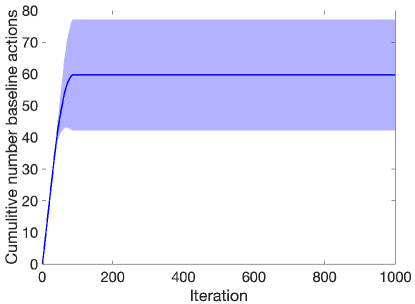
Figure 2: Cumulative number of times that the baseline actions played by SCLTS up to time $t$, for $t=1\dots,1000$ over 100 realizations.

Appendix E Upper Bounding the Regret of SCLTS-BF

In this section we provide the variation of our algorithm for the case of constraints with bandit feedback, which we refer to as SCLTS-BF in Algorithm 2. We then provide a regret bound for SCLTS-BF. The summary of SCLTS-BF is presented in Algorithm 2.

1

2

3Input: $\delta,T,\lambda,\rho$

4Set $\delta^{\prime}=\frac{\delta}{4T}$

5 for $t=1,\dots,T$  do

6       Sample $\eta_{t}\sim\mathcal{H}^{\text{TS}}$

7      

8      Compute RLS-estimate $\hat{\theta}_{t}$ and $V_{t}$ according to (5) and $\hat{\mu}_{t}$

9      Set $\tilde{\theta}_{t}=\hat{\theta}_{t}+\beta_{t}V_{t}^{-1/2}\eta_{t}$

10      

11      Build the confidence region $\mathcal{E}_{t}(\delta^{\prime})$ in (55) and $\mathcal{C}_{t}(\delta^{\prime})$ in (56)

12      Compute the estimated safe set $\mathcal{P}_{t}^{s}=\{x\in\mathcal{X}:\langle x,v\rangle\geq(1-\alpha)q_{b_{t}},\forall v\in\mathcal{C}_{t}\}$

13      

14      if the following optimization has a feasible solution: $x(\tilde{\theta}_{t})=\text{argmax}_{x\in\mathcal{P}_{t}^{s}}\langle x,\tilde{\theta}_{t}\rangle$, then

15      Set $F=1$, else $F=0$

16      

17      if $F=1$ and $\lambda_{\text{min}}(V_{t})\geq\left(\frac{2L\beta_{t}}{\nu_{l}+\alpha q_{l}}\right)^{2}$, then

18      Play $x_{t}=x(\tilde{\theta}_{t})$

19      else

20      play $x_{t}=x_{t}^{\text{cb}}$ defined in (59)

21      Observe reward $r_{t}$

22      

end for

Algorithm 2 SCLTS-BF

In this setting, we assume that at each round $t$, with playing an action $x_{t}$, the learner observes the reward $y_{t}=\langle x_{t},\theta_{\star}\rangle+\xi_{t}$ and the following bandit feedback:

$$w_{t}=\langle x_{t},\mu_{\star}\rangle+\chi_{t},$$ (54)

where $\chi_{t}$ is assumed to be a zero-mean $R$-sub-Gaussian noise.

The main difference of SCLTS-BF with SCLTS is in the definition of the estimated safe action set. In particular, at each round $t$, SCLTS-BF constructs the following confidence regions:

$$\mathcal{E}_{t}(\delta^{\prime})=\{\theta\in\mathbb{R^{d}}:\left\lVert\theta-\hat{\theta}_{t}\right\rVert_{V_{t}}\leq\beta_{t}(\delta^{\prime})\},$$ (55)

$$\mathcal{C}_{t}(\delta^{\prime})=\{v\in\mathbb{R^{d}}:\left\lVert v-\hat{\mu}_{t}\right\rVert_{V_{t}}\leq\beta_{t}(\delta^{\prime})\},$$ (56)

where $\hat{\mu}_{t}=V_{t}^{-1}\sum_{s=1}^{t-1}w_{s}x_{s}$ is the RLS-estimate of $\mu_{\star}$. The radius in (55) and (56) is chosen according to Proposition 2.1 such that $\theta_{\star}\in\mathcal{E}_{t}$ and $\mu_{\star}\in\mathcal{C}_{t}$ with high probability. In order to ensure safety at each round $t$, SCLTS-BF constructs the following estimated safe action set

$$\mathcal{P}_{t}^{s}=\{x\in\mathcal{X}:\langle x,v\rangle\geq(1-\alpha)q_{b_{t}},\forall v\in\mathcal{C}_{t}\}.$$ (57)

The challenge with $\mathcal{P}_{t}^{s}$ is that it contains all the actions that are safe with respect to all the parameters in $\mathcal{C}_{t}$. Thus, there may exist some rounds that $\mathcal{P}_{t}^{s}$ is empty. To handle this case, SCLTS-BF proceed as follows. At each round $t$, given the sampled parameter $\tilde{\theta}_{t}$, if the estimated safe action set $\mathcal{P}_{t}^{s}$ defined in (57) is not empty, SCLTS-BF plays the safe action

$$x(\tilde{\theta}_{t})=\arg\max_{x\in\mathcal{P}_{t}^{s}}\langle x,\tilde{\theta}_{t}\rangle$$ (58)

only if $\lambda_{\text{min}}(V_{t})\geq k^{2}_{t}$, where $k^{2}_{t}=\left(\frac{2L\beta_{t}}{\nu_{l}+\alpha q_{l}}\right)^{2}$. Otherwise, it plays the following conservative action

$$x_{t}^{\text{cb}}=(1-\rho_{2})x_{b_{t}}+\rho_{2}\zeta_{t},$$ (59)

where $\rho_{2}=\alpha(\frac{q_{l}}{S+q_{h}})$ in order to ensure that the conservative actions are safe.

Next, we provide a regret guarantee for SCLTS-BF. First, we use the following decomposition of regret:

$$R(T) =\sum_{t=1}^{T}\langle x_{\star},\theta_{\star}\rangle-\langle x_{t},\theta_{\star}\rangle$$

$$=\underbrace{\sum_{t\in N_{T}}\bigg{(}\langle x_{\star},\theta_{\star}\rangle-\langle x_{t},\theta_{\star}\rangle\bigg{)}}_{\text{Term I}}+\underbrace{\sum_{t\in N_{T}^{c}}\bigg{(}\langle x_{\star},\theta_{\star}\rangle-\langle(1-\rho)x_{b_{t}}-\rho\zeta_{t},\theta_{\star}\rangle\bigg{)}}_{\text{Term II}},$$ (60)

where $N_{t}^{c}$ is the set of rounds $i<t$ that SCLTS-BF plays the conservative actions, and $N_{t}=\{1,\dots,t\}-N_{t}^{c}$. In the following, we upper bound both Term I and Term II, separately.

Bounding Term I. Bounding Term I follows the same steps as that of Theorem 3.2. Here, we show that for SCLTS-BF, at rounds $t\in N_{T}$, the optimal action $x_{\star}$ belongs to the estimated safe safe, i.e., $x_{\star}\in\mathcal{P}_{t}^{s}$. Then, we conclude that regret of Term I similar to Theorem 3.2 has the order of $\mathcal{O}(d^{3/2}\log^{1/2}d\leavevmode\nobreak\ T^{1/2}\log^{3/2}T)$.

At rounds $t\in N_{T}$, we know

$$\lambda_{\text{min}}(V_{t})\geq k_{t}^{2}\geq\left(\frac{2L\beta_{t}}{\nu_{b_{t}}+\alpha q_{b_{t}}}\right)^{2}.$$ (61)

Then, in order to show that $x_{\star}\in\mathcal{X}_{t}^{s}$, we need to show

$$\langle x_{\star},\hat{\mu}_{t}\rangle-\beta_{t}\|x_{\star}\|_{V_{t}^{-1}}\geq\langle x_{\star},\mu_{\star}\rangle-2\beta_{t}\|x_{\star}\|_{V_{t}^{-1}}\geq(1-\alpha)q_{b_{t}}.$$ (62)

First inequality comes from the fact that $\|\mu_{\star}-\hat{\mu}_{t}\|_{V_{t}}\leq\beta_{t}$. Therefore, it suffices to show the second inequality holds. We use the fact that $\|x_{\star}\|_{V_{t}^{-1}}\leq\frac{\|x_{\star}\|_{2}}{\sqrt{\lambda_{\text{min}}(V_{t})}}\leq\frac{L}{\sqrt{\lambda_{\text{min}}(V_{t})}}$, where we use Assumption 3 to bound $\|x_{\star}\|_{2}$. Hence, we have

$$\langle x_{\star},\mu_{\star}\rangle-2\beta_{t}\|x_{\star}\|_{V_{t}^{-1}}\geq\langle x_{\star},\mu_{\star}\rangle-\frac{2\beta_{t}L}{\sqrt{\lambda_{\text{min}}(V_{t})}}.$$ (63)

Then, it suffices to show that

$$\nu_{b_{t}}+\alpha q_{b_{t}}\geq\frac{2\beta_{t}L}{\sqrt{\lambda_{\text{min}}(V_{t})}},$$ (64)

From (61), we know that (64) holds, and hence, $x_{\star}\in\mathcal{P}_{t}^{s}$. Therefore, we can use the result of Theorem 3.2, and obtain the desired regret bound.

Bounding Term II. First, we provide the formal statement of the theorem.

Theorem E.1.

Let $\lambda,L\geq 1$. On event $\bigg{\{}\{\theta_{\star}\in\mathcal{E}_{t},\forall t\in[T]\}\cap\{\mu_{\star}\in\mathcal{C}_{t},\forall t\in[T]\}\bigg{\}}$, and Assumptions 4, we can upper bound the number of times SCLTS-BF plays the conservative actions, i.e., $|N_{T}^{c}|$ as:

$$|N_{T}^{c}|\leq\left(\frac{2L\beta_{T}}{\rho_{2}\sigma_{\zeta}(\alpha q_{l}+\nu_{l})}\right)^{2}+\frac{2h_{2}^{2}}{\rho_{2}^{4}\sigma_{\zeta}^{4}}\log(\frac{d}{\delta})+\frac{2Lh_{2}\beta_{T}\sqrt{8\log(\frac{d}{\delta})}}{\rho_{2}^{3}\sigma_{\zeta}^{3}(\alpha q_{l}+\nu_{l})}$$ (65)

where $h_{2}=2\rho_{2}(1-\rho_{2})L+2\rho_{2}^{2}$ and $\rho_{2}=(\frac{q_{l}}{S+q_{h}})\alpha$.

In order to prove Theorem E.1, we proceed as follows:

$$\sum_{t\in N_{T}^{c}}\bigg{(}\langle x_{\star},\theta_{\star}\rangle-\langle(1-\rho_{2})x_{b_{t}}-\rho_{2}\zeta_{t},\theta_{\star}\rangle\bigg{)} =\sum_{t\in N_{T}^{c}}\langle x_{\star},\theta_{\star}\rangle-\langle x_{b_{t}},\theta_{\star}\rangle+\rho_{2}(\langle x_{b_{t}}+\zeta_{t},\theta_{\star}\rangle)$$

$$\leq\sum_{t\in N_{T}^{c}}\nu_{h}+\rho_{2}(q_{b_{t}}+S)\leq|N_{T}^{c}|(\nu_{h}+\alpha q_{l}),$$ (66)

where $q_{h}\geq q_{b_{t}}\geq q_{l}>0$ and $\nu_{h}\geq\nu_{b_{t}}\geq\nu_{l}$ for all $t$. Therefore, in order to bound Term II, it suffices to upper bound $|N_{T}^{c}|$ which is the number of rounds that SCLTS-BF plays the conservative actions up to round T. In order to do so, we proceed as follows:

Let $\tau$ be any round that the algorithm plays the conservative action.

If $F=0$, i.e.,

$$\nexists x\in\mathcal{X}:\langle x,\hat{\mu}_{\tau}\rangle-\beta_{\tau}\|x\|_{V_{\tau}^{-1}}\geq(1-\alpha)q_{b_{\tau}},$$ (67)

and since we know that $x_{\star}\in\mathcal{X}$, and $\mu_{\star}\in\mathcal{C}_{t}$ with high probability, we can write

$$\langle x_{\star},\mu_{\star}\rangle-2\beta_{\tau}\|x_{\star}\|_{V_{\tau}^{-1}}\leq\langle x_{\star},\hat{\mu}_{\tau}\rangle-\beta_{\tau}\|x_{\star}\|_{V_{\tau}^{-1}}<(1-\alpha)q_{b_{\tau}}.$$ (68)

Using (68), we can get

$$\nu_{b_{\tau}}+\alpha q_{b_{\tau}}<2\beta_{\tau}\|x_{\star}\|_{V_{\tau}^{-1}}\leq\frac{2\beta_{\tau}L}{\sqrt{\lambda_{\text{min}}(V_{\tau})}},$$ (69)

and hence the following upper bound on minimum eigenvalue of the Gram matrix:

$$\lambda_{\text{min}}(V_{\tau})<\left(\frac{2\beta_{\tau}L}{\nu_{b_{\tau}}+\alpha q_{b_{\tau}}}\right)^{2}\leq\left(\frac{2\beta_{\tau}L}{\nu_{l}+\alpha q_{l}}\right)^{2}=k_{\tau}$$ (70)

Therefore, we show that in the cases where either the event $\{\nexists x\in\mathcal{X}:\langle x,\hat{\mu}_{\tau}\rangle-\beta_{\tau}\|x\|_{V_{\tau}^{-1}}\geq(1-\alpha)q_{b_{\tau}}\}$ or the event $\{\lambda_{\text{min}}(V_{\tau})<k_{\tau}^{2}\}$ happen, we can conclude that at round $\tau$

$$\lambda_{\text{min}}(V_{\tau})<k_{\tau}^{2}.$$ (71)

From Lemma D.1, we know that the minimum eigenvalue of the Gram matrix, i.e., $\lambda_{\text{min}}(V_{t})$ is lower bounded with the number of times that SCLTS-BF plays the conservative actions, i.e., $|N_{T}^{c}|$. Therefore, using (71), we can get

$$|N_{T}^{c}|\leq\left(\frac{2L\beta_{T}}{\rho_{2}\sigma_{\zeta}(\alpha q_{l}+\nu_{l})}\right)^{2}+\frac{2h_{2}^{2}}{\rho_{2}^{4}\sigma_{\zeta}^{4}}\log(\frac{d}{\delta})+\frac{2Lh_{2}\beta_{T}\sqrt{2\log(\frac{d}{\delta})}}{\rho_{2}^{3}\sigma^{3}(\alpha q_{l}+\nu_{l})}$$ (72)

where $h_{2}=2\rho_{2}(1-\rho_{2})L+2\rho_{2}^{2}$ and $\rho_{2}=\alpha(\frac{q_{l}}{S+q_{h}})$.

Appendix F Proof of Theorem 4.1

In this section, we first present the SCLTS2 algorithm, for the case where the learner does not know the reward of the actions suggested by baseline policy in advance, i.e., $r_{b_{t}}$. The summary of SCLTS2 is presented in Algorithm 3.

The algorithm relies on the fact that we can find an upper bound over the value of $r_{b_{t}}$, using the fact that $\theta_{\star}\in\mathcal{E}_{t}$, i.e.,:

$$\max_{v\in\mathcal{E}_{t}}\langle x_{b_{t}},v\rangle\geq\langle x_{b_{t}},\theta_{\star}\rangle=r_{b_{t}}.$$ (73)

Then, we can write the safety constraint as follows:

$$\min_{v\in\mathcal{E}_{t}}\langle x(\tilde{\theta}_{t}),v\rangle\geq(1-\alpha)\max_{v\in\mathcal{E}_{t}}\langle x_{b_{t}},v\rangle.$$ (74)

It is easy to show that safety constraint (2) holds when (74) is true. Therefore, if we choose actions that satisfy (74), we can ensure that they are safe with respect to the safety constrain in (2).

Then we propose the estimated safe action set $\mathcal{Z}_{t}^{s}$ as:

$$\mathcal{Z}_{t}^{s} =\{x\in\mathcal{X}:\min_{v\in\mathcal{E}_{t}}\langle x,v\rangle\geq(1-\alpha)\max_{v\in\mathcal{E}_{t}}\langle x_{b_{t}},v\rangle\},$$ (75)

which contains actions that are safe with respect to all the parameter in $\mathcal{E}_{t}$. At each round $t$, SCLTS2 plays the safe action $x(\tilde{\theta}_{t})$ from $\mathcal{Z}_{t}^{s}$ that maximizes the expected reward given the sampled parameter $\tilde{\theta}_{t}$, i.e.,

$$x(\tilde{\theta}_{t})=\arg\max_{x\in\mathcal{Z}_{t}^{s}}\langle x,\tilde{\theta}_{t}\rangle$$ (76)

only if $\lambda_{\text{min}}(V_{t})\geq k_{t}^{3}$, where $k_{t}^{3}=\left(\frac{2L\beta_{t}(2-\alpha)}{\kappa_{l}+\alpha r_{l}}\right)^{2}$. Otherwise it plays the conservative action $x_{b_{t}}^{\text{cb}}$ as:

$$x_{t}^{\text{cb}}=(1-\rho_{3})x_{b_{t}}+\rho_{3}\zeta_{t},$$ (77)

where $\rho_{3}=\alpha(\frac{r_{l}}{S+1})$ such that the conservative action $x_{t}^{\text{cb}}$ is safe, where we use Assumption 3 for upper bounding the reward, i.e., $r_{b_{t}}\leq 1$.

1

2

3Input: $\delta,T,\lambda,\rho$

4Set $\delta^{\prime}=\frac{\delta}{4T}$

5 for $t=1,\dots,T$  do

6       Sample $\eta_{t}\sim\mathcal{H}^{\text{TS}}$

7      

8      Compute RLS-estimate $\hat{\theta}_{t}$ and $V_{t}$ according to (5)

9      Set $\tilde{\theta}_{t}=\hat{\theta}_{t}+\beta_{t}V_{t}^{-1/2}\eta_{t}$

10      

11      Build the confidence region $\mathcal{E}_{t}(\delta^{\prime})$ in (6)

12      Compute the estimated safe set $\mathcal{Z}_{t}^{s}=\{x\in\mathcal{X}:\min_{v\in\mathcal{E}_{t}}\langle x,v\rangle\geq(1-\alpha)\max_{v\in\mathcal{E}_{t}}\langle x_{b_{t}},v\rangle\}$

13      

14      if the following optimization is feasible: $x(\tilde{\theta}_{t})=\arg\max_{x\in\mathcal{Z}_{t}^{s}}\langle x,\tilde{\theta}_{t}\rangle$, then

15      Set $F=1$, else $F=0$

16      

17      if $F=1$ and $\lambda_{\text{min}}(V_{t})\geq\left(\frac{2L\beta_{t}(2-\alpha)}{\kappa_{l}+\alpha r_{l}}\right)^{2}$, then

18      Play $x_{t}=x(\tilde{\theta}_{t})$

19      else

20      play $x_{t}=x_{t}^{\text{cb}}$ defined in (77)

21      Observe reward $y_{t}$

22      

end for

Algorithm 3 SCLTS2

In order to bound the regret of SCLTS2, we first use the decomposition defined in Proposition 3.1. The regret of Term I is similar to that of SCLTS (i.e., Theorem 3.2). Hence, it suffices to upper bound the number of time SCLTS2 plays the conservative actions, i.e., $|N_{T}^{c}|$.

In order to bound $|N_{T}^{c}|$, we proceed as follows. Let $\tau$ be the round that SCLTS2 plays a conservative action. If $F=0$, i.e.,

$$\nexists x\in\mathcal{X}:\min_{v\in\mathcal{C}_{\tau}}\langle x,v\rangle\geq(1-\alpha)\max_{v\in\mathcal{C}_{\tau}}\langle x_{b_{\tau}},v\rangle.$$ (78)

Using the fact that $x_{\star}\in\mathcal{X}$, we can write

$$\langle x_{\star},\hat{\theta}_{\tau}\rangle-\beta_{\tau}\|x_{\star}\|_{V_{\tau}^{-1}}<(1-\alpha)\left(\langle x_{b_{\tau}},\hat{\theta}_{\tau}\rangle+\beta_{\tau}\|x_{b_{\tau}}\|_{V_{\tau}^{-1}}\right).$$ (79)

Then, since $\|\theta_{\star}-\hat{\theta}_{t}\|_{V_{t}}\leq\beta_{t}$, we can upper bound the RHS and lower bound the LHS of (79), and get

$$\langle x_{\star},{\theta}_{\star}\rangle-2\beta_{\tau}\|x_{\star}\|_{V_{\tau}^{-1}}<(1-\alpha)\left(\langle x_{b_{\tau}},{\theta}_{\star}\rangle+2\beta_{\tau}\|x_{b_{\tau}}\|_{V_{\tau}^{-1}}\right),$$ (80)

or equivalently,

$$\kappa_{b_{\tau}}+\alpha r_{b_{\tau}}<2\beta_{\tau}\|x_{\star}\|_{V_{\tau}^{-1}}+2(1-\alpha)\beta_{\tau}\|x_{b_{\tau}}\|_{V_{\tau}^{-1}}.$$ (81)

Then we can use the fact that $\|x_{\star}\|_{V_{\tau}^{-1}}\leq\frac{L}{\sqrt{\lambda_{\text{min}}(V_{\tau})}}$ and $\|x_{b_{\tau}}\|_{V_{\tau}^{-1}}\leq\frac{L}{\sqrt{\lambda_{\text{min}}(V_{\tau})}}$, where we use Assumption 3 for upper bounding $\|x_{\star}\|_{2}$. Thus, we upper bound the RHS of (81) as follows:

$$\kappa_{b_{\tau}}+\alpha r_{b_{\tau}}<2\beta_{\tau}\frac{L}{\sqrt{\lambda_{\text{min}}(V_{\tau})}}+2(1-\alpha)\beta_{\tau}\frac{L}{\sqrt{\lambda_{\text{min}}(V_{\tau})}},$$ (82)

and hence, we can get the following upper bound ${\lambda_{\text{min}}(V_{\tau})}$ as follows:

$${\lambda_{\text{min}}(V_{\tau})}<\left(\frac{2L\beta_{T}(2-\alpha)}{\kappa_{b_{\tau}}+\alpha r_{b_{\tau}}}\right)^{2}\leq\left(\frac{2L\beta_{T}(2-\alpha)}{\kappa_{l}+\alpha r_{l}}\right)^{2}=k_{\tau}^{3}.$$ (83)

Therefore, we show that whether the event $F=0$ happens or ${\lambda_{\text{min}}(V_{t})}<k_{t}^{3}$, we can achieve the upper bound provided in (83). Then, using the result of Lemma D.1, where we show that ${\lambda_{\text{min}}(V_{t})}$ is lower bounded with the number of times the algorithm plays the conservative actions, we obtain the following upper bound on the $|N_{\tau}^{c}|$

$$|N_{\tau}^{c}|\leq\left(\frac{2L\beta_{\tau}(2-\alpha)}{\rho_{3}\sigma_{\zeta}(\kappa_{l}+\alpha r_{l})}\right)^{2}+\frac{2h_{3}^{2}}{\rho_{3}^{4}\sigma_{\zeta}^{4}}\log(\frac{d}{\delta})+\frac{2Lh_{3}\beta_{\tau}(2-\alpha)}{\rho_{3}^{3}\sigma_{\zeta}^{3}(\kappa_{l}+\alpha r_{l})}\sqrt{2\log(\frac{d}{\delta})},$$ (84)

where $h_{3}=2\rho_{3}(1-\rho_{3})L+2\rho_{3}^{2}$ and $\rho_{3}=\alpha(\frac{r_{l}}{S+1})$.

Appendix G Stage-wise Conservative Linear UCB (SCLUCB) Algorithm

In this section we propose a UCB-based safe stochastic linear bandit algorithm called Stage-wise Conservative Linear-UCB (SCLUCB), which is a safe counterpart of LUCB for the stage-wise conservative bandit setting. In particular, at each round $t$, given the RLS-estimate $\hat{\theta}_{t}$ of $\theta_{\star}$, SCLUCB constructs the confidence region $\mathcal{E}_{t}$ as follows:

$$\mathcal{E}_{t}(\delta)=\{\theta\in\mathbb{R}^{d}:\|\theta-\hat{\theta}_{t}\|_{V_{t}}\leq\beta_{t}(\delta)\}.$$ (85)

The radius $\beta_{t}(\delta)$ is chosen as in Proposition 2.1 such that $\theta_{\star}\in\mathcal{E}_{t}(\delta)$ with probability $1-\delta$. Then, similar to SCLTS, it builds the estimated safe set $\mathcal{X}_{t}^{s}$ such that it includes actions that are safe with respect to all the parameter in $\mathcal{E}_{t}$, i.e.,

$$\mathcal{X}_{t}^{s}=\{x\in\mathcal{X}:\langle x,v\rangle\geq(1-\alpha)r_{b_{t}},\forall v\in\mathcal{E}_{t}\}.$$ (86)

Similar to SCLTS, the challenge with $\mathcal{X}_{t}^{s}$ is that there may exist some rounds that $\mathcal{X}_{t}^{s}$ is empty. In order to face this problem, SCLUCB proceed as follows. In order to guarantee safety, at each round $t$, if $\mathcal{X}_{t}^{s}$ is not empty, SCLUCB plays the action $\bar{x}_{t}$ as

$$(\bar{x}_{t},\bar{\theta}_{t})=\max_{x\in\mathcal{X}_{t}^{s}}\max_{v\in\mathcal{E}_{t}}\langle x,v\rangle$$ (87)

only if $\lambda_{\text{min}}(V_{t})\geq\left(\frac{2L\beta_{t}}{\kappa_{l}+\alpha r_{b_{l}}}\right)^{2}$, otherwise it plays the conservative action $x_{t}^{\text{cb}}$ defined in (11). The summary of SCLUCB is presented in Algorithm (4).

1

2

3Input: $\delta,T,\lambda,\rho$

4for $t=1,\dots,T$  do

5      

6      Compute RLS-estimate $\hat{\theta}_{t}$ and $V_{t}$ according to (5)

7      Build the confidence region $\mathcal{E}_{t}(\delta)$ in (85)

8      Compute the estimated safe set $\mathcal{X}_{t}^{s}$ in (86)

9      

10      if the following optimization is feasible: $\bar{x}_{t}=\arg\max_{x\in\mathcal{X}_{t}^{s}}\max_{v\in\mathcal{E}_{t}}\langle x,v\rangle$, then

11      Set $F=1$, else $F=0$

12      

13      if $F=1$ and $\lambda_{\text{min}}(V_{t})\geq\left(\frac{2L\beta_{t}}{\kappa_{l}+\alpha r_{b_{l}}}\right)^{2}$, then

14      Play $x_{t}=\bar{x}_{t}$

15      else

16      play $x_{t}=x_{t}^{\text{cb}}$ defined in (11)

17      Observe reward $y_{t}$

18      

end for

Algorithm 4 Stage-wise Conservative Linear UCB (SCLUCB)

Next, we provide the regret guarantee for SCLUCB. Recall, $N_{t-1}$ be the set of rounds $i<t$ at which SCLUCB plays the action in (10). Similarly, $N_{t-1}^{c}=\{1,\dots,t-1\}-N_{t-1}$ is the set of rounds $j<t$ at which SCLUCB plays the conservative actions.

Proposition G.1.

The regret of SCLUCB can be decomposed into two terms as follows:

$$R(T)\leq\underbrace{\sum_{t\in N_{T}}\left(\langle x_{\star},\theta_{\star}\rangle-\langle x_{t},\theta_{\star}\rangle\right)}_{\text{Term I}}+\underbrace{|N_{T}^{{c}}|\left(\kappa_{h}+\rho_{1}(r_{h}+S)\right)}_{\text{Term II}}$$ (88)

In the following, we bound both terms, separately.

Bounding Term I. The first Term in (88) is the regret caused by playing the safe actions that maximize the reward given the true parameter is $\bar{\theta}_{t}$. The idea of bounding Term I is similar to Abbasi-Yadkori et al., (2011). We use the fact that for $t\in N_{T}$, $x_{t}=\bar{x}_{t}$, and start with the following decomposition of the instantaneous regret for $t\in N_{T}$ :

$$\langle x_{\star},\theta_{\star}\rangle-\langle x_{t},\theta_{\star}\rangle=\underbrace{\langle x_{\star},\theta_{\star}\rangle-\langle\bar{x}_{t},\bar{\theta}_{t}\rangle}_{\text{Term A}}+\underbrace{\langle\bar{x}_{t},\bar{\theta}_{t}\rangle-\langle\bar{x}_{t},\theta_{\star}\rangle}_{\text{Term B}}$$ (89)

Bounding Term A. Since for round $t\in N_{t}$, we require that $\lambda_{\text{min}}(V_{t})\geq k_{t}^{1}$, where $k_{t}^{1}=\left(\frac{2L\beta_{t}}{\kappa_{l}+\alpha r_{b_{l}}}\right)^{2}$, we can conclude that $x_{\star}\in\mathcal{X}_{t}^{s}$. Therefore, due to (87), we have $\langle\bar{x}_{t},\bar{\theta}_{t}\rangle\geq\langle x_{\star},\theta_{\star}\rangle$, and hence Term A is not positive.

Bounding Term B. In order to bound Term B, we use the following chain of inequalities:

Term B $$:=\langle\bar{x}_{t},\bar{\theta}_{t}\rangle-\langle\bar{x}_{t},\theta_{\star}\rangle=\langle\bar{x}_{t},\bar{\theta}_{t}\rangle-\langle\bar{x}_{t},\hat{\theta}_{t}\rangle+\langle\bar{x}_{t},\hat{\theta}_{t}\rangle-\langle\bar{x}_{t},\theta_{\star}\rangle$$

$$\leq\|\bar{x}_{t}\|_{V_{t}^{-1}}\|\bar{\theta}_{t}-\hat{\theta}_{t}\|_{V_{t}}+\|\bar{x}_{t}\|_{V_{t}^{-1}}\|\hat{\theta}_{t}-\theta_{\star}\|_{V_{t}}$$

$$\leq 2\beta_{t}\|\bar{x}_{t}\|_{V_{t}^{-1}},$$ (90)

where the last inequality follows from Proposition 2.1. Recall, from Assumption 3, we have the following trivial bound:

$$\langle x_{\star},\theta_{\star}\rangle-\langle\bar{x}_{t},\theta_{\star}\rangle\leq 2.$$ (91)

Thus, we conclude the following

$$\text{Term B}\leq 2\min(\beta_{t}\|\bar{x}_{t}\|_{V_{t}^{-1}},1).$$ (92)

Next, we state a direct application of Lemma 11 in Abbasi-Yadkori et al., (2011).

Lemma G.2.

For $\lambda>0$, and under Assumptions 1, 2, and 3, we have

$$\sum_{t=1}^{T}\min(\|\bar{x}_{t}\|^{2}_{V_{t}^{-1}},1)\leq 2d\log\left(1+\frac{TL^{2}}{\lambda d}\right)$$ (93)

Therefore, from Lemma G.2, we can conclude the following bound on regret of Term B:

$$\sum_{t\in N_{T}}2\min(\beta_{t}\|\bar{x}_{t}\|_{V_{t}^{-1}},1)\leq 2\beta_{T}\sqrt{2d|N_{T}|\log(1+\frac{|N_{T}|L^{2}}{\lambda d})}.$$ (94)

Next, in Theorem G.3, we provide an upper bound on the regret of Term I which is of order $\mathcal{O}\left(d\sqrt{T}\log(\frac{TL^{2}}{\lambda\delta})\right)$.

Theorem G.3.

On event $\{\theta_{\star}\in\mathcal{E}_{t}\}$ for a fixed $\delta\in(0,1)$, with probability $1-\delta$, it holds that:

$$\sum_{t\in N_{T}}\left(\langle x_{\star},\theta_{\star}\rangle-\langle x_{t},\theta_{\star}\rangle\right)\leq 2\beta_{T}\sqrt{2dT\log(1+\frac{TL^{2}}{\lambda d})}$$ (95)

Bounding Term II. In order to bound Term II in (88), we need to find an upper bound on the number of times that SCLUCB plays the conservative actions up to time $T$, i.e., $|N_{T}^{c}|$. We prove an upper bound on $|N_{T}^{c}|$ in Theorem G.4 which has the order of $\mathcal{O}\left(\frac{L^{2}d\log(\frac{T}{\delta})\log(\frac{d}{\delta})}{\alpha^{4}(r_{l}^{2}\wedge r_{l}^{4})\kappa_{l}(\sigma_{\zeta}^{2}\wedge\sigma_{\zeta}^{4})}\right)$.

Theorem G.4.

Let $\lambda,L\geq 1$. On event $\{\theta_{\star}\in\mathcal{E}_{t},\forall t\in[T]\}$, and under Assumption 4, we can upper bound the number of times SCLUCB plays the conservative actions, i.e., $|N_{T}^{c}|$ as:

$$|N_{T}^{c}|\leq\left(\frac{2L\beta_{T}}{\rho_{1}\sigma_{\zeta}(\kappa_{l}+\alpha r_{l})}\right)^{2}+\frac{2h_{1}^{2}}{\rho_{1}^{4}\sigma_{\zeta}^{4}}\log(\frac{d}{\delta})+\frac{2Lh_{1}\beta_{T}\sqrt{8\log(\frac{d}{\delta})}}{\rho_{1}^{3}\sigma^{3}(\kappa_{l}+\alpha r_{l})},$$ (96)

where $h_{1}=2\rho_{1}(1-\rho_{1})L+2\rho_{1}^{2}$ and $\rho_{1}=(\frac{r_{l}}{S+r_{h}})\alpha$.

The proof is similar to that of Theorem 3.3, and we omit its proof here.

Appendix H Comparison with Safe-LUCB

In this section, we extend our results to an alternative safe bandit formulation proposed in Amani et al., (2019), where the algorithm Safe-LUCB was proposed. In order to do so, we first present the safety constraint in Amani et al., (2019), and then we show the required modification of SCLUCB to handle this case, which we refer to as SCLUCB2. Then, we provide a problem-dependent regret bound for SCLUSB2, and we show that it matches the problem dependent regret bound of Safe-LUCB in Amani et al., (2019). We need to note that in Amani et al., (2019), they also provide a general regret bound of order $\tilde{\mathcal{O}}({T^{2/3}})$ for Safe-LUCB which we do not discuss in this paper.

In Amani et al., (2019), it is assumed that the learner is given a convex and compact decision set $\mathcal{D}_{0}$ which contains the origin, and with playing the action $x_{t}$, she observes the reward of $y_{t}=x_{t}^{\top}\theta_{\star}+\eta_{t}$, where $\theta_{\star}$ is the fixed unknown parameter, and $\eta_{t}$ is $R$-sub-Gaussian noise. Moreover, The learning environment is subject to the linear safety constraint

$$x^{\top}B\theta_{\star}\leq C,$$ (97)

which needs to be satisfied at all rounds $t$ with high probability, and an action $x_{t}$ is called safe, if it satisfies (97). In (97), the matrix $B\in\mathbb{R}^{d\times d}$ and the positive constant $C$ are known to the learner. However, the learner does not receive any bandit feedback on the value $x^{\top}B\theta_{\star}$ and her information is restricted to those she receives from the reward.

Given the above constraint, the learner is restricted to choose actions from the safe set $\mathcal{D}_{0}^{s}$ as:

$$\mathcal{D}_{0}^{s}(\theta_{\star})=\{x\in\mathcal{D}_{0}:x^{\top}B\theta_{\star}\leq C\}.$$ (98)

Since $\theta_{\star}$ in unknown, the safe set $\mathcal{D}_{0}^{s}$ is unknown to the learner. Then, in Amani et al., (2019), they provide the problem-dependent regret bound (for the case where $\Delta:=C-x^{\top}B\theta_{\star}>0$) of order $\mathcal{O}(\sqrt{T}\log T)$. In the following, we present the required modification of SCLUSB to handle this safe bandit formulation, and propose the new algorithm called SCLUCB2 that we prove a problem dependnt regret bound of order $\mathbb{O}(\sqrt{T}\log T)$. We need to note that Amani et al., (2019) also provide a general regret bound of order $\tilde{\mathcal{O}}({T^{2/3}})$ for the case where $\Delta=0$; however, we do not discuss this case in this paper.

At each round $t$, given the RLS-estimate $\hat{\theta}_{t}$ of $\theta_{\star}$, SLUCB2 builds the confidence region $\mathcal{E}_{t}$ as:

$$\mathcal{E}_{t}=\{\theta\in\mathbb{R}^{d}:\|\theta-\hat{\theta}_{t}\|_{V_{t}}\leq\beta_{t}\},$$ (99)

and the radius $\beta_{t}$ is chosen according to Proposition 2.1 such that $\theta_{\star}\in\mathcal{E}_{t}$ with high probability. The learner does not know the safe set $\mathcal{D}_{0}^{s}$; however, she knows that $\theta_{\star}\in\mathcal{E}_{t}$ with high probability. Hence, SLUCB2 constructs the estimated safe set $\mathcal{D}_{t}^{s}$ such that it contains actions that are safe with respect to all the parameter in $\mathcal{E}_{t}$, i.e.,

$$\mathcal{D}_{t}^{s} =\{x\in\mathcal{D}_{0}:x^{\top}Bv\leq C,\forall v\in\mathcal{E}_{t}\}$$

$$=\{x\in\mathcal{D}_{0}:\max_{v\in\mathcal{E}_{t}}x^{\top}Bv\leq C\}$$

$$=\{x\in\mathcal{D}_{0}:x^{\top}B\hat{\theta}_{t}+\beta_{t}\|Bx\|_{V_{t}^{-1}}\leq C\}$$ (100)

Clearly, action $x=[0]^{d}$ (origin) is a safe action since $C>0$, and also $[0]^{d}\in\mathcal{D}_{0}$. Thus, $[0]^{d}\in\mathcal{D}_{t}^{s}$. Since $x=[0]^{d}$ is a known safe action, we define the conservative action $x_{0}^{\text{c}}$ as:

$$x_{0}^{\text{c}}=(1-\rho)[0]^{d}+\rho\zeta_{t}=\rho\zeta_{t},$$ (101)

where $\zeta_{t}$ is a sequence of IID random vectors such that $\|\zeta_{t}\|_{2}=1$ almost surly, and $\sigma_{\zeta}=\lambda_{\text{min}}(\text{Cov}(\zeta_{t}))>0$. We choose the constant $\rho$ according to the Lemma H.1 in order to ensure that the conservative action $x_{0}^{\text{c}}$ is safe.

Lemma H.1.

At each round $t$, for any $\rho\in(0,\bar{\rho})$, where

$$\bar{\rho}=\frac{C}{\|B\|S},$$ (102)

the conservative action $x_{0}^{\text{c}}=\rho\zeta_{t}$ is guaranteed to be safe almost surly.

We choose $\rho=\frac{C}{\|B\|S}$ for the rest of this section, and hence the conservative action is

$$x_{0}^{\text{c}}=\frac{C}{\|B\|S}\zeta_{t}.$$ (103)

Let $\Delta=C-x_{\star}^{\top}B\theta_{\star}$. We consider the case where $\Delta>0$. At each $t$, in order to guarantee safety, SCLUCB2 only chooses its action from the estimated safe set $\mathcal{D}_{t}^{s}$. The challenge with $\mathcal{D}_{t}^{s}$ is that it includes actions that are safe with respect to all parameter in $\mathcal{E}_{t}$, and not only $\theta_{\star}$. Thus, there may exist some rounds that $\mathcal{D}_{t}^{s}$ is empty. At round $t$, if $\mathcal{D}_{t}^{s}$ is not empty, SCLUCB2 plays the safe action

$$\bar{x}_{t}=\arg\max_{x\in\mathcal{D}_{t}^{s}}\max_{v\in\mathcal{E}_{t}}\langle x,v\rangle$$ (104)

only if $\lambda_{\text{min}}(V_{t})\geq\left(\frac{2L\beta_{t}\|B\|}{\Delta}\right)^{2}$, otherwise it plays the conservative action $x_{0}^{\text{c}}$ in (103). The summary of SCLUCB2 is presented in Algorithm 5.

1

2

3Input: $\delta,T,\lambda,\rho$

4for $t=1,\dots,T$  do

5      

6      Compute RLS-estimate $\hat{\theta}_{t}$ and $V_{t}$ according to (5)

7      Build the confidence region $\mathcal{E}_{t}(\delta)$ in (99)

8      Compute the estimated safe set $\mathcal{D}_{t}^{s}$ in (100)

9      

10      if the following optimization is feasible: $\bar{x}_{t}=\arg\max_{x\in\mathcal{D}_{t}^{s}}\max_{v\in\mathcal{E}_{t}}\langle x,v\rangle$, then

11      Set $F=1$, else $F=0$

12      

13      if $F=1$ and $\lambda_{\text{min}}(V_{t})\geq\left(\frac{2L\beta_{t}\|B\|}{\Delta}\right)^{2}$, then

14      Play $x_{t}=\bar{x}_{t}$

15      else

16      play $x_{t}=x_{0}^{\text{c}}$ defined in (103)

17      Observe reward $y_{t}$

18      

end for

Algorithm 5 SCLUCB2

In the following we provide the regret guarantee for SCLUCB2. Let $N_{t-1}$ be the set of rounds $i<t$ at which SCLUCB2 plays the action in (104). Similarly, $N_{t-1}^{c}=\{1,\dots,t-1\}-N_{t-1}$ is the set of rounds $j<t$ at which SCLUCB2 plays the conservative action in (103).

First, we use the following decomposition of the regret, then we bound each term separately.

Proposition H.2.

The regret of SCLUCB2 can be decomposed to the following two terms:

$$R(T) =\sum_{t=1}^{T}\langle x_{\star},\theta_{\star}\rangle-\langle x_{t},\theta_{\star}\rangle$$

$$={\sum_{t\in N_{T}}\bigg{(}\langle x_{\star},\theta_{\star}\rangle-\langle x_{t},\theta_{\star}\rangle\bigg{)}}+{\sum_{t\in N_{T}^{c}}\bigg{(}\langle x_{\star},\theta_{\star}\rangle-\langle x_{0}^{\text{c}},\theta_{\star}\rangle\bigg{)}},$$

$$\leq\underbrace{\sum_{t\in N_{T}}\bigg{(}\langle x_{\star},\theta_{\star}\rangle-\langle x_{t},\theta_{\star}\rangle\bigg{)}}_{\text{Term I}}+\underbrace{2|N_{t}^{c}|}_{\text{Term II}}.$$ (105)

Bounding Term I. In order to bound Term I, we proceed as follows. First, we show that at rounds $t\in N_{T}$, the optimal action $x_{\star}$ belongs to the estimated safe set $\mathcal{D}_{t}^{s}$, i.e., $x_{\star}\in\mathcal{D}_{t}^{s}$. To do so, we need to show that

$$x_{\star}^{\top}B\hat{\theta}_{t}+\beta_{t}\|Bx_{\star}\|_{V_{t}^{-1}}\leq C.$$ (106)

Since $\|\theta_{\star}-\hat{\theta}_{t}\|_{V_{t}}\leq\beta_{t}$, it suffices to show that:

$$x_{\star}^{\top}B\theta_{\star}+2\beta_{t}\|Bx_{\star}\|_{V_{t}^{-1}}\leq C,$$ (107)

or equivalently

$$2\beta_{t}\|Bx_{\star}\|_{V_{t}^{-1}}\leq\Delta,$$ (108)

where $\Delta=C-x_{\star}^{\top}B\theta_{\star}$. It is easy to see (106) is true whenever (107) holds. Using Assumption 3, we can get $\|Bx_{\star}\|_{V_{t}^{-1}}\leq\frac{\|B\|\|x_{\star}\|_{2}}{\sqrt{\lambda_{\text{min}}(V_{t})}}\leq\frac{\|B\|L}{\sqrt{\lambda_{\text{min}}(V_{t})}}$. Hence, from (108), it suffices to show that

$$\frac{2\beta_{t}\|B\|L}{\sqrt{\lambda_{\text{min}}(V_{t})}}\leq\Delta,$$ (109)

or equivalently

$$\lambda_{\text{min}}(V_{t})\geq\left(\frac{2\beta_{t}\|B\|L}{\Delta}\right)^{2}$$ (110)

that we know it is true for $t\in N_{T}$. Therefore, on event $\{\theta_{\star}\in\mathcal{E}_{t}\}$, $x_{\star}\in\mathcal{D}_{t}^{s}$. We can bound the regret of Term I in (105) similar to Theorem G.3, and get the regret of order $\mathcal{O}\left(d\sqrt{T}\log(\frac{TL^{2}}{\lambda\delta})\right)$.

Bounding Term II. We need to upper bound the number of times that SCLUCB2 plays the conservative action $x_{0}^{\text{c}}$, i.e., $|N_{T}^{c}|$. We prove an upper bound on $|N_{T}^{c}|$ in Theorem H.3 which has the order of $\mathcal{O}\left(\frac{L^{2}S^{2}\|B\|^{2}d\log(\frac{T}{\delta})\log(\frac{d}{\delta})}{\Delta^{2}(C\wedge C^{2})(\sigma_{\zeta}^{2}\wedge\sigma_{\zeta}^{4})}\right)$.

Theorem H.3.

Let $\lambda,L\geq 1$. On event $\{\theta_{\star}\in\mathcal{E}_{t},\forall t\in[T]\}$, we can upper bound the number of times SCLUCB2 plays the conservative actions, i.e., $|N_{T}^{c}|$ as:

$$|N_{T}^{c}|\leq\left(\frac{2LS\|B\|^{2}\beta_{T}}{C\Delta\sigma_{\zeta}}\right)^{2}+\frac{32\log(\frac{d}{\delta})}{\sigma_{\zeta}^{4}}+\frac{8LS\|B\|^{2}\beta_{T}\sqrt{2\log(\frac{d}{\delta})}}{C\Delta\sigma_{\zeta}^{3}}.$$ (111)

Proof.

Let $\tau$ be any round that the algorithm plays the conservative action, i.e., at round $\tau$, either $F=0$ or $\lambda_{\text{min}}(V_{\tau})<\left(\frac{2L\|B\|\beta_{\tau}}{\Delta}\right)^{2}$.

By definition, if $F=0$, we have

$$\nexists x\in\mathcal{X}:x^{\top}B\hat{\theta}_{\tau}+\beta_{\tau}\|Bx\|_{V_{\tau}^{-1}}\leq C,$$ (112)

and since we know that $x_{\star}\in\mathcal{X}$, and $\theta_{\star}\in\mathcal{E}_{t}$ with high probability, we can write

$$x_{\star}^{\top}B\theta_{\star}+2\beta_{\tau}\|Bx_{\star}\|_{V_{\tau}^{-1}}\geq\ x_{\star}^{\top}B\hat{\theta}_{\tau}+\beta_{\tau}\|Bx_{\star}\|_{V_{\tau}^{-1}}>C.$$ (113)

Then, using the LHS and RHS of (113), we can get

$$\frac{2L\|B\|\beta_{\tau}}{\sqrt{\lambda_{\text{min}}(V_{\tau})}}\geq 2\beta_{\tau}\|x_{\star}\|_{V_{\tau}^{-1}}\geq\Delta,$$

and hence the following upper bound on minimum eigenvalue of the Gram matrix:

$$\lambda_{\text{min}}(V_{\tau})<\left(\frac{2L\|B\|\beta_{\tau}}{\Delta}\right)^{2}.$$

Therefore, at any round $\tau$ that a conservative action is played, whether it is because $\{F=0\}$ happens or beccause we have $\{\lambda_{\text{min}}(V_{\tau})<\left(\frac{2L\|B\|\beta_{\tau}}{\Delta}\right)^{2}\}$, we can always conclude that

$$\lambda_{\text{min}}(V_{\tau})<\left(\frac{2L\|B\|\beta_{\tau}}{\Delta}\right)^{2}$$ (114)

The remaining of the proof builds on two auxiliary lemmas. First, in Lemma H.4, we show that the minimum eigenvalue of the Gram matrix $V_{t}$ is lower bounded with the number of times SCLUCB2 plays the conservative actions.

Lemma H.4.

On event $\{\theta_{\star}\in\mathcal{E}_{t}\}$, it holds that

$$\mathbb{P}(\lambda_{\text{min}}(V_{t})\leq t)\leq d\exp{\left(-\frac{(\rho^{2}\sigma_{\zeta}^{2}|N_{t}^{c}|-t)^{2}}{32\rho^{4}|N_{t}^{c}|}\right)},$$ (115)

where $\rho=\frac{C}{\|B\|S}$.

Using (114) and applying Lemma H.4, it can checked that with probability $1-\delta$

$$\left(\frac{2L\|B\|\beta_{\tau}}{\Delta}\right)^{2}>\rho^{2}\sigma_{\zeta}^{2}|N_{\tau}^{c}|-\sqrt{32\rho^{4}.|N_{\tau}^{c}|\log(\frac{d}{\delta})},$$

Then using Lemma D.2, we can conclude the following upper bound

$$|N_{\tau}^{c}|\leq\left(\frac{2LS\|B\|^{2}\beta_{\tau}}{C\Delta\sigma_{\zeta}}\right)^{2}+\frac{32\log(\frac{d}{\delta})}{\sigma_{\zeta}^{4}}+\frac{8LS\|B\|^{2}\beta_{\tau}\sqrt{2\log(\frac{d}{\delta})}}{C\Delta\sigma_{\zeta}^{3}}.$$

∎

H.1 Proof of Lemma H.4

Our objective is to establish a lower bound on $\lambda_{\text{min}}(V_{t})$ for all $t$. It holds that

$$V_{t} =\lambda I+\sum_{s=1}^{t}x_{s}x_{s}^{\top}$$

$$\succeq\sum_{s\in N_{t}^{c}}\left(\rho\zeta_{s}\right)\left(\rho\zeta_{s}\right)^{\top}$$

$$=\sum_{s\in N_{t}^{c}}\bigg{(}\rho^{2}\mathbb{E}[\zeta_{s}\zeta_{s}^{\top}]+\rho^{2}\zeta_{s}\zeta_{s}^{\top}-\rho^{2}\mathbb{E}[\zeta_{s}\zeta_{s}^{\top}]\bigg{)}$$

$$\succeq\rho^{2}\sigma_{\zeta}^{2}|N_{t}^{c}|I+\sum_{s\in N_{t}^{c}}G_{s},$$ (116)

where $G_{s}$ is defined as

$$G_{s}=\bigg{(}\rho^{2}\zeta_{s}\zeta_{s}^{\top}-\rho^{2}\mathbb{E}[\zeta_{s}\zeta_{s}^{\top}]\bigg{)}.$$ (117)

Thus, using Weyl’s inequality, it follows that

$$\lambda_{\text{min}}(V_{t})\geq\rho^{2}\sigma_{\zeta}^{2}|N_{t}^{c}|-\lambda_{\text{max}}(\sum_{s\in N_{t}^{c}}G_{s}).$$

Next, we apply the matrix Azuma inequality (see Theorem D.3) to find an upper bound on $\lambda_{\text{max}}(\sum_{s\in N_{t}^{c}}G_{s})$. For this, we first need to show that the sequence of matrices $G_{s}$ satisfies the conditions of Theorem D.3. By definition of $G_{s}$ in (117), it follows that $\mathbb{E}[G_{s}|\mathcal{F}_{s-1}]=0$, and $G_{s}^{\top}=G_{s}$. Also, we construct the sequence of deterministic matrices $A_{s}$ such that $G_{s}^{2}\preceq A_{s}^{2}$ as follows. We know that for any matrix $K$, $K^{2}\leq\|K\|_{2}^{2}I$, where $\|K\|_{2}$ is the maximum singular value of $K$, i.e.,

$$\sigma_{\text{max}}(K)=\max_{\|u\|_{1}=\|v\|_{2}=1}u^{\top}Kv.$$

Thus, we first show the following bound on the maximum singular value of the matrix $G_{s}$ defined in (117):

$$\max_{\|u\|_{1}=\|v\|_{2}=1}u^{\top}G_{s}v =\rho^{2}(u^{\top}\zeta_{s})(v^{\top}\zeta_{s})^{\top}-\rho^{2}\mathbb{E}\left[(u^{\top}\zeta_{s})(v^{\top}\zeta_{s})^{\top}\right]$$

$$\leq\rho^{2}\|\zeta_{s}\|_{2}^{2}+\rho^{2}\mathbb{E}\left[\|\zeta_{s}\|_{2}^{2}\right]$$

$$\leq 2\rho^{2},$$

where we have used Cauchy-Schwarz inequality and the last inequality comes from the fact that $\|\zeta_{s}\|_{2}=1$ almost surely. From the derivations above, and choosing $A_{s}=2\rho^{2}I$, it almost surely holds that $G_{s}^{2}\preceq\sigma_{\text{max}}(G_{s})^{2}I\preceq 4\rho^{4}I=A_{s}^{2}$. Moreover, using triangular inequality, it holds that

$$\|\sum_{s\in N_{t}^{c}}A_{s}^{2}\|\leq\sum_{s\in N_{t}^{c}}\|A_{s}^{2}\|\leq 4\rho^{4}|N_{t}^{c}|.$$

Now we can apply the matrix Azuma inequality, to conclude that for any $c\geq 0$,

$$\mathbb{P}\left(\lambda_{\text{max}}(\sum_{s\in N_{t}^{c}}G_{s})\geq c\right)\leq d\exp{\left(-\frac{c^{2}}{32\rho^{4}|N_{t}^{c}|}\right)}.$$

Therefore, it holds that with probability $1-\delta$, $\lambda_{\text{max}}(\sum_{s\in N_{t}^{c}}G_{s})\leq\sqrt{32\rho^{4}|N_{t}^{c}|\log(\frac{d}{\delta})}$, and hence with probability $1-\delta$,

$$\lambda_{\text{min}}(V_{t})\geq\rho^{2}\sigma_{\zeta}^{2}|N_{t}^{c}|-\sqrt{32\rho^{4}|N_{t}^{c}|\log(\frac{d}{\delta})},$$ (118)

or equivalently,

$$\mathbb{P}(\lambda_{\text{min}}(V_{t})\leq t)\leq d\exp{\left(-\frac{(\rho^{2}\sigma_{\zeta}^{2}|N_{t}^{c}|-t)^{2}}{32\rho^{4}|N_{t}^{c}|}\right)},$$ (119)

where $\rho=\frac{C}{\|B\|S}$. This completes the proof.

H.2 Simulation Results

In order to verify our results on the regret bound of SCLUCB2, we plot the Figure 3 which plots the cumulative regret of the two algorithms averaged over $100$ realizations. Therefore, the regret of SCLUCB2 matches the proposed problem-dependent upper bound in Amani et al., (2019).

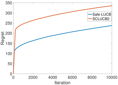
Figure 3: Cumulative regret of SCLUCB2 versus Safe-LUCB in Amani et al., (2019) averaged over $100$ realizations.

References

• Abbasi-Yadkori etΒ al., (2011) Abbasi-Yadkori, Y., PΓ‘l, D., and SzepesvΓ‘ri, C. (2011). Improved algorithms for linear stochastic bandits. In Advances in Neural Information Processing Systems, pages 2312–2320.
• Abeille etΒ al., (2017) Abeille, M., Lazaric, A., etΒ al. (2017). Linear thompson sampling revisited. Electronic Journal of Statistics, 11(2):5165–5197.
• Agrawal and Goyal, (2013) Agrawal, S. and Goyal, N. (2013). Thompson sampling for contextual bandits with linear payoffs. In International Conference on Machine Learning, pages 127–135.
• Akametalu etΒ al., (2014) Akametalu, A.Β K., Fisac, J.Β F., Gillula, J.Β H., Kaynama, S., Zeilinger, M.Β N., and Tomlin, C.Β J. (2014). Reachability-based safe learning with gaussian processes. In 53rd IEEE Conference on Decision and Control, pages 1424–1431.
• Amani etΒ al., (2019) Amani, S., Alizadeh, M., and Thrampoulidis, C. (2019). Linear stochastic bandits under safety constraints. In Advances in Neural Information Processing Systems, pages 9252–9262.
• Aswani etΒ al., (2013) Aswani, A., Gonzalez, H., Sastry, S.Β S., and Tomlin, C. (2013). Provably safe and robust learning-based model predictive control. Automatica, 49(5):1216–1226.
• Auer etΒ al., (2002) Auer, P., Cesa-Bianchi, N., and Fischer, P. (2002). Finite-time analysis of the multiarmed bandit problem. Mach. Learn., 47(2-3):235–256.
• Bubeck and Eldan, (2016) Bubeck, S. and Eldan, R. (2016). Multi-scale exploration of convex functions and bandit convex optimization. In Conference on Learning Theory, pages 583–589.
• Dani etΒ al., (2008) Dani, V., Hayes, T.Β P., and Kakade, S.Β M. (2008). Stochastic linear optimization under bandit feedback.
• Filippi etΒ al., (2010) Filippi, S., Cappe, O., Garivier, A., and SzepesvΓ‘ri, C. (2010). Parametric bandits: The generalized linear case. In Advances in Neural Information Processing Systems, pages 586–594.
• Katariya etΒ al., (2018) Katariya, S., Kveton, B., Wen, Z., and Potluru, V.Β K. (2018). Conservative exploration using interleaving. arXiv preprint arXiv:1806.00892.
• Kaufmann etΒ al., (2012) Kaufmann, E., Korda, N., and Munos, R. (2012). Thompson sampling: An asymptotically optimal finite-time analysis. In International Conference on Algorithmic Learning Theory, pages 199–213. Springer.
• Kazerouni etΒ al., (2017) Kazerouni, A., Ghavamzadeh, M., Abbasi, Y., and VanΒ Roy, B. (2017). Conservative contextual linear bandits. In Guyon, I., Luxburg, U.Β V., Bengio, S., Wallach, H., Fergus, R., Vishwanathan, S., and Garnett, R., editors, Advances in Neural Information Processing Systems 30, pages 3910–3919. Curran Associates, Inc.
• Khezeli and Bitar, (2019) Khezeli, K. and Bitar, E. (2019). Safe linear stochastic bandits. arXiv preprint arXiv:1911.09501.
• Koller etΒ al., (2018) Koller, T., Berkenkamp, F., Turchetta, M., and Krause, A. (2018). Learning-based model predictive control for safe exploration. In 2018 IEEE Conference on Decision and Control (CDC), pages 6059–6066. IEEE.
• Li etΒ al., (2017) Li, L., Lu, Y., and Zhou, D. (2017). Provably optimal algorithms for generalized linear contextual bandits. In Proceedings of the 34th International Conference on Machine Learning-Volume 70, pages 2071–2080. JMLR. org.
• Mansour etΒ al., (2015) Mansour, Y., Slivkins, A., and Syrgkanis, V. (2015). Bayesian incentive-compatible bandit exploration. In Proceedings of the Sixteenth ACM Conference on Economics and Computation, pages 565–582.
• Moradipari etΒ al., (2020) Moradipari, A., Alizadeh, M., and Thrampoulidis, C. (2020). Linear thompson sampling under unknown linear constraints. In ICASSP 2020 - 2020 IEEE International Conference on Acoustics, Speech and Signal Processing (ICASSP), pages 3392–3396.
• Moradipari etΒ al., (2019) Moradipari, A., Amani, S., Alizadeh, M., and Thrampoulidis, C. (2019). Safe linear thompson sampling with side information. arXiv, page arXiv:1911.02156.
• Moradipari etΒ al., (2018) Moradipari, A., Silva, C., and Alizadeh, M. (2018). Learning to dynamically price electricity demand based on multi-armed bandits. In 2018 IEEE Global Conference on Signal and Information Processing (GlobalSIP), pages 917–921. IEEE.
• Ostafew etΒ al., (2016) Ostafew, C.Β J., Schoellig, A.Β P., and Barfoot, T.Β D. (2016). Robust constrained learning-based nmpc enabling reliable mobile robot path tracking. The International Journal of Robotics Research, 35(13):1547–1563.
• Rusmevichientong and Tsitsiklis, (2010) Rusmevichientong, P. and Tsitsiklis, J.Β N. (2010). Linearly parameterized bandits. Mathematics of Operations Research, 35(2):395–411.
• Russo and VanΒ Roy, (2016) Russo, D. and VanΒ Roy, B. (2016). An information-theoretic analysis of thompson sampling. The Journal of Machine Learning Research, 17(1):2442–2471.
• Sui etΒ al., (2018) Sui, Y., Burdick, J., Yue, Y., etΒ al. (2018). Stagewise safe bayesian optimization with gaussian processes. In International Conference on Machine Learning, pages 4788–4796.
• Sui etΒ al., (2015) Sui, Y., Gotovos, A., Burdick, J.Β W., and Krause, A. (2015). Safe exploration for optimization with gaussian processes. In Proceedings of the 32Nd International Conference on International Conference on Machine Learning - Volume 37, ICML’15, pages 997–1005. JMLR.org.
• Thompson, (1933) Thompson, W.Β R. (1933). On the likelihood that one unknown probability exceeds another in view of the evidence of two samples. Biometrika, 25(3/4):285–294.
• Tropp, (2012) Tropp, J.Β A. (2012). User-friendly tail bounds for sums of random matrices. Foundations of computational mathematics, 12(4):389–434.
• Tucker etΒ al., (2020) Tucker, N., Moradipari, A., and Alizadeh, M. (2020). Constrained thompson sampling for real-time electricity pricing with grid reliability constraints. IEEE Transactions on Smart Grid, pages 1–1.
• Wu etΒ al., (2016) Wu, Y., Shariff, R., Lattimore, T., and SzepesvΓ‘ri, C. (2016). Conservative bandits. In International Conference on Machine Learning, pages 1254–1262.