Non-parametric regression for networks

Abstract

Network data are becoming increasingly available, and so there is a need to develop suitable methodology for statistical analysis. Networks can be represented as graph Laplacian matrices, which are a type of manifold-valued data. Our main objective is to estimate a regression curve from a sample of graph Laplacian matrices conditional on a set of Euclidean covariates, for example in dynamic networks where the covariate is time. We develop an adapted Nadaraya-Watson estimator which has uniform weak consistency for estimation using Euclidean and power Euclidean metrics. We apply the methodology to the Enron email corpus to model smooth trends in monthly networks and highlight anomalous networks. Another motivating application is given in corpus linguistics, which explores trends in an author’s writing style over time based on word co-occurrence networks.

1 Introduction

Networks are of wide interest and able to represent many different phenomena, for example social interactions and connections between regions in the brain (Kolaczyk,, 2009; Ginestet et al.,, 2017). The study of dynamic networks has recently increased as more data of this type is becoming available (Rastelli et al.,, 2018), where networks evolve over time. In this paper we develop some non-parametric regression methods for modelling and predicting networks where covariates are available. An application for this work is the study of dynamic networks derived from the Enron email corpus, in which each network corresponds to communications between employees in a particular month (Diesner et al.,, 2005). Another motivating application is the study of evolving writing styles in the novels of Jane Austen and Charles Dickens, in which each network is a representation of a novel based on word co-occurences, and the covariate is the time that writing of the novel began (Severn et al.,, 2020). In both applications, the goal is to model smooth trends in the structure of the dynamic networks as they evolve over time.

An example of previous work on dynamic network data is Friel et al., (2016) who embedded nodes of bipartite dynamic networks in a latent space, motivated by networks representing the connection of leading Irish companies and board directors. We will also use embeddings in our work, although the bipartite constraints are not present. Further approaches include object functional principal components analysis (Dubey and Mueller,, 2019) applied to time-varying networks from New York taxi trip data; multi-scale time-series modelling (Kang et al.,, 2017) applied to magnetoencephalography data in neuroscience; and quotient space space methodology applied to brain arterial networks (Guo and Srivastava,, 2020).

The analysis of networks is a type of object oriented data analysis (Marron and Alonso,, 2014), and important considerations are to decide what are the data objects and how are they represented. We consider datasets where each observation is a weighted network, denoted $G_{m}=(V,E)$, comprising a set of nodes, $V=\{v_{1},v_{2},\ldots,v_{m}\}$, and a set of edge weights, $E=\{w_{ij}:w_{ij}\geq 0,1\leq i,j\leq m\}$, indicating nodes $v_{i}$ and $v_{j}$ are either connected by an edge of weight $w_{ij}>0$, or else unconnected (if $w_{ij}=0$). An unweighted network is the special case with $w_{ij}\in\{0,1\}$. We restrict attention to networks that are undirected and without loops, so that $w_{ij}=w_{ji}$ and $w_{ii}=0$, then any such network can be identified with its graph Laplacian matrix $\mathbf{L}=(l_{ij})$, defined as

$$l_{ij}=\begin{cases}-w_{ij},&\text{if }i\neq j\\ \sum_{k\neq i}w_{ik},&\text{if }i=j\end{cases}$$

for $1\leq i,j\leq m$. The graph Laplacian matrix can be written as $\mathbf{L}=\mathbf{D}-\mathbf{A}$, in terms of the adjacency matrix, $\mathbf{A}=(w_{ij})$, and degree matrix $\mathbf{D}=\text{diag}(\sum_{j=1}^{m}w_{1j},\ldots,\sum_{j=1}^{m}w_{mj})=\text{diag}(\mathbf{A}\mathbf{1}_{m})$, where $\mathbf{1}_{m}$ is the $m$-vector of ones. The $i$th diagonal element of $\mathbf{D}$ equals the degree of node $i$. The space of $m\times m$ graph Laplacian matrices is of dimension $m(m-1)/2$ and is

$$\mathcal{L}_{m}=\{\mathbf{L}=(l_{ij}):\mathbf{L}=\mathbf{L}^{T};\,l_{ij}\leq 0\,\forall i\neq j;\,\mathbf{L}{\mathbf{1}_{m}}={\mathbf{0}_{m}}\},$$ (1)

where $\mathbf{0}_{m}$ is the $m$-vector of zeroes. In fact the space $\mathcal{L}_{m}$ is a closed convex subset of the cone of centred symmetric positive semi-definite $m\times m$ matrices and $\mathcal{L}_{m}$ is a manifold with corners (Ginestet et al.,, 2017).

Since the sample space $\mathcal{L}_{m}$ for graph Laplacian data is non-Euclidean, standard approaches to non-parametric regression cannot be applied directly. In this paper, we use the statistical framework introduced in Severn et al., (2020) for extrinsic analysis of graph Laplacian data, in which “extrinsic” refers to the strategy of mapping data into a Euclidean space, where analysis is performed, before mapping back to $\mathcal{L}_{m}$. The choice of mapping enables freedom in the choice of metric used for the statistical analysis, and in various applications with manifold-valued data analysis there is evidence of advantage in using non-Euclidean metrics (Dryden et al.,, 2009; Pigoli et al.,, 2014).

A summary of the key steps in the extrinsic approach is:

1. embedding to another manifold ${\mathcal{M}}_{m}$ by raising the graph Laplacian matrix to a power,

2. mapping from $\mathcal{M}_{m}$ to a (Euclidean) tangent space $T_{\nu}(\mathcal{M}_{m})$ in which to carry out statistical analysis,

3. inverse mapping from the tangent space $T_{\nu}(\mathcal{M}_{m})$ to the embedding manifold $\mathcal{M}_{m}$,

4. reversing the powering in i), and projecting back to graph Laplacian space $\mathcal{L}_{m}$,

which we explain in more detail as follows. First write $\mathbf{L}=\mathbf{U}\boldsymbol{\Xi}\mathbf{U}^{T}$ by the spectral decomposition theorem, with $\boldsymbol{\Xi}=\text{diag}(\xi_{1},\ldots,\xi_{m})$ and $\mathbf{U}=(\mathbf{u}_{1},\ldots,\mathbf{u}_{m})$, where $\{\xi_{i}\}_{i=1,\ldots,m}$ are the eigenvalues, which are non-negative as any $\mathbf{L}$ is positive semi-definite, and $\{\mathbf{u}_{i}\}_{i=1,\ldots,m}$ are the corresponding eigenvectors of $\mathbf{L}$. We consider the following map which raises the graph Laplacian to the power $\alpha>0$:

$$\begin{split}\text{F}_{\alpha}(\mathbf{L})&=\mathbf{L}^{\alpha}=\mathbf{U}\boldsymbol{\Xi}^{\alpha}\mathbf{U}^{T}:\mathcal{L}_{m}\rightarrow\operatorname{Image}(\mathcal{L}_{m})\subset\mathcal{M}_{m}.\\ \end{split}$$ (2)

In this paper we take ${\cal M}_{m}$ to be the Euclidean space of symmetric $m\times m$ matrices. In terms of $\text{F}_{\alpha}(\cdot)$ we define the power Euclidean distance between two graph Laplacians as

$$d_{\alpha}(\mathbf{L}_{1},\mathbf{L}_{2})=\|\text{F}_{\alpha}(\mathbf{L}_{1})-\text{F}_{\alpha}(\mathbf{L}_{2})\|,$$ (3)

where $\|\mathbf{X}\|=\sqrt{{\rm trace}(\mathbf{X}^{T}\mathbf{X})}$ is the Frobenius norm, also known as the Euclidean norm. For the special case $\alpha=1$, (3) is just the Euclidean distance. Severn et al., (2020) further considered a Procrustes distance which includes minimization over an orthogonal matrix, approximately allowing relabelling of the nodes, and in this case the embedding manifold $\mathcal{M}_{m}$ is a Riemannian manifold known as the size-and-shape space (Dryden and Mardia,, 2016, p.99). However, in this paper for simplicity and because the labelling is known, we shall just consider the power Euclidean metric.

After the embedding the data are mapped to a tangent space $T_{\nu}(\mathcal{M}_{m})$ of the embedding manifold at $\nu$ using the bijective transformation

$$\pi_{\nu}^{-1}:\mathcal{M}_{m}\to T_{\nu}(\mathcal{M}_{m}).$$

In our applications we take $\nu=0$ and the tangent co-ordinates are $\mathbf{v}={\rm vech}(\mathbf{H}\text{F}_{\alpha}(\mathbf{L})\mathbf{H}^{T})$, where ${\rm vech}()$ is the vector of elements above and including the diagonal and $\mathbf{H}$ is the Helmert sub-matrix (Dryden and Mardia,, 2016, p49). The main point of note is that the tangent space is a Euclidean space of dimension $m(m-1)/2$. Hence, multivariate linear statistical analysis can be carried out in $T_{\nu}(\mathcal{M}_{m})$; for example, Severn et al., (2020) considered estimation, two-sample hypothesis tests, and linear regression.

After carrying out statistical analysis, the fitted values are then transformed back to the graph Laplacian space as follows:

$$P_{\cal L}\circ\text{G}_{\alpha}\circ\pi_{\nu}:T_{\nu}(\mathcal{M}_{m})\to\mathcal{L}_{m}$$ (4)

where $\text{G}_{\alpha}:\mathcal{M}_{m}\to\mathcal{M}_{m}$ is a map that reverses the power, and $P_{\cal L}:\mathcal{M}_{m}\to\mathcal{L}_{m}$ is the projection to the closest point in graph Laplacian space using Euclidean distance. The projection $P_{\cal L}$ is obtained by solving a convex optimization problem using quadratic programming, and the solution is therefore unique. See Severn et al., (2020) for full details of this framework.

For visualising results, it is useful to map the data and fitted regression lines in $\mathcal{L}_{m}$ into $\mathbb{R}^{2}$. In this paper we do so using principal component analysis (PCA) such that the two plotted dimensions reflect the two orthogonal dimensions of greatest sample variability in the tangent space (Severn et al.,, 2020).

2 Nadaraya-Watson estimator for network data

2.1 Nadaraya-Watson estimator

We first review the classical Nadaraya-Watson estimator (Watson,, 1964; Nadaraya,, 1965) before defining an analogous version for data on $\mathcal{L}_{m}$. Consider the regression problem where we want to predict an unknown variable $y(\mathbf{x})\in\mathbb{R}$ with known covariate $\mathbf{x}\in\mathbb{R}^{p}$ for the dataset of independent and identically distributed random variables $(\{Y_{1},\mathbf{X}_{1}\},\dots,\{Y_{n},\mathbf{X}_{n}\})$ observed at $(\{y_{1},\mathbf{x}_{1}\},\dots,\{y_{n},\mathbf{x}_{n}\})$ with $E\{|Y|\}<\infty$. The aim is to estimate the regression function

$$m(\mathbf{x})=E[y(\mathbf{x})|\mathbf{x}].$$

The Nadaraya-Watson estimator is

$$\hat{m}(\mathbf{x})=\frac{\sum_{i=1}^{n}K_{h}(\mathbf{x}-\mathbf{x}_{i})y_{i}}{\sum_{i=1}^{n}K_{h}(\mathbf{x}-\mathbf{x}_{i})},$$ (5)

where $K_{h}\geq 0$ is a kernel function with bandwidth $h>0$.

Consider now a version of the regression problem with $y(\mathbf{x})$ replaced with an $m\times m$ graph Laplacian matrix $\mathbf{L}(\mathbf{x})\in\mathcal{L}_{m}$ with known covariates $\mathbf{x}\in\mathbb{R}^{p}$ and dataset $(\{\mathbf{L}_{1},\mathbf{x}_{1}\},\dots,\{\mathbf{L}_{n},\mathbf{x}_{n}\})$ with $E\{|(\mathbf{L})_{ij}|\}<\infty,i=1,\ldots,m;j=1,\ldots,m$. We wish to estimate the regression function

$$\boldsymbol{\Lambda}(x)=E[\mathbf{L}(\mathbf{x})|\mathbf{x}].$$

A natural analogue of $\hat{m}(\mathbf{x})$ in (5) for graph Laplacian data given covariate, $\mathbf{x}\in\mathbb{R}^{p}$, is

$$\hat{\mathbf{L}}_{NW}(\mathbf{x})=\frac{\sum_{i=1}^{n}K_{h}(\mathbf{x}-\mathbf{x}_{i})\mathbf{L}_{i}}{\sum_{i=1}^{n}K_{h}(\mathbf{x}-\mathbf{x}_{i})}=\sum_{i=1}^{n}W_{hi}(\mathbf{x})\mathbf{L}_{i},$$ (6)

where

$$W_{hi}(\mathbf{x})=\frac{K_{h}(\mathbf{x}-\mathbf{x}_{i})}{\sum_{i=1}^{n}K_{h}(\mathbf{x}-\mathbf{x}_{i})}\geq 0$$

and note that $\sum_{i=1}^{n}W_{hi}(\mathbf{x})=1$. A common choice of kernel function is the Gaussian kernel

$$K_{h}(\mathbf{u})=\frac{1}{h\sqrt{2\pi}}\exp\left(-\frac{\|\mathbf{u}\|^{2}}{2h^{2}}\right),$$ (7)

which is bounded above and strictly positive for all $\mathbf{u}$. We use a truncated version of (7) such that $K_{h}(\mathbf{u})=0$ for $\|\mathbf{u}\|>c$ (with $c$ large) in order that this truncated kernel has compact support, as required by theoretical results presented later. Wherever $\hat{\mathbf{L}}_{NW}$ is defined (meaning that at least one of the $K_{h}(\mathbf{x}-\mathbf{x}_{i})$ is non-zero) it is a sum of positively weighted graph Laplacians. Since the space $\mathcal{L}_{m}$ is a convex cone (Ginestet et al.,, 2017), itself defined as the sum of positively weighted graph Laplacians, thus $\hat{\mathbf{L}}_{NW}(\mathbf{t})\in\mathcal{L}_{m}$ as required.

The estimator in (6) can equivalently be written as the graph Laplacian that minimises a weighted sum of squared Euclidean, $d_{1}$, distances to the sample data

$$\hat{\mathbf{L}}_{NW}(\mathbf{x})=\arg\inf_{{\mathbf{L}}\in\mathcal{L}_{m}}\sum_{i=1}^{n}W_{hi}(\mathbf{x})d_{1}(\mathbf{L}_{i},\boldsymbol{\mathbf{L}})^{2}=\arg\inf_{{\mathbf{L}}\in\mathcal{L}_{m}}\sum_{i=1}^{n}W_{hi}(\mathbf{x})\|\mathbf{L}_{i}-\boldsymbol{\mathbf{L}}\|^{2},$$ (8)

using weighted least squares. In principle, the Euclidean distance $d_{1}$ in $\eqref{eq:manifold nadaraya euc}$ can be replaced with a different distance metric, $d$, though solving for the estimator entails an optimisation on the manifold $\mathcal{L}_{m}$, which can be theoretically and computationally challenging. Hence instead we generalise to other distances via an extrinsic approach, and define

$$\hat{\mathbf{L}}_{NW,d}(\mathbf{x})=\text{P}_{\mathcal{L}}\left(\arg\inf_{\boldsymbol{\mathbf{L}}\in\mathcal{M}_{m}}\sum_{i=1}^{n}W_{hi}(\mathbf{x})d(\mathbf{L}_{i},\boldsymbol{\mathbf{L}})^{2}\right),$$ (9)

which is simpler provided, as here, the embedding manifold $\mathcal{M}_{m}$ is chosen such that the optimisation is straightforward. The projection is needed to map back to graph Laplacian space ${\cal L}_{m}$. For the power Euclidean metric, $d_{\alpha}$, consider the Nadaraya-Watson estimator in the tangent space $T_{\nu}({\cal M}_{m})$,

$$\hat{\mathbf{L}}_{{\cal M}_{m},\alpha}(\mathbf{x})=\sum_{i=1}^{n}W_{hi}(\mathbf{x})\pi_{\nu}^{-1}(\text{F}_{\alpha}(\mathbf{L}_{i})),$$ (10)

in terms of which, after mapping back to ${\mathcal{L}}_{m}$ using (4), the resulting Nadaraya-Watson estimator in the graph Laplacian space is

$$\hat{\mathbf{L}}_{NW,\alpha}(\mathbf{x})=P_{\cal L}\circ\text{G}_{\alpha}\circ\pi_{\nu}\left(\hat{\mathbf{L}}_{{\cal M}_{m},\alpha}(\mathbf{x})\right).$$ (11)

When $\alpha=1$ this simplifies to (6).

2.2 Uniform weak consistency

First we show that the Nadaraya-Watson estimator for graph Laplacians (6) is uniformly weakly consistent.

Let

$$J_{n}=E\left\{\int\left\|\hat{\mathbf{L}}_{NW}(\mathbf{x})-\boldsymbol{\Lambda}(\mathbf{x})\right\|^{2}\mu(\mathrm{d}\mathbf{x})\right\}$$ (12)

where $\mu$ is the probability measure of $\mathbf{x}$.

Proposition 1.

Suppose the kernel function $K_{h}$ is non-negative on $\mathbb{R}^{p}$, bounded above, has compact support and is strictly positive in a neighbourhood of the origin. If $E\{\|\mathbf{L}\|^{2}\}<\infty$, as $h\to 0$ and $nh^{d}\to\infty$ it follows that $J_{n}\to 0$. Hence the Nadaraya-Watson estimator $\hat{\mathbf{L}}_{NW}(\mathbf{x})$ is uniformly weakly consistent for the true regression function $\boldsymbol{\Lambda}(\mathbf{x})$.

Proof.

Consider the univariate regression problem for the $(i,j)$th element of $\hat{\mathbf{L}}_{NW}(\mathbf{x})$. From Devroye and Wagner, (1980) we know that under the conditions of the proposition we have

$$J_{n,ij}=E\left\{\int\left|\left(\hat{\mathbf{L}}_{NW}(\mathbf{x})\right)_{ij}-\left(\boldsymbol{\Lambda}(\mathbf{x})\right)_{ij}\right|^{2}\mu(\mathrm{d}\mathbf{x})\right\}\to 0\;,\;i=1,\ldots,m;j=1,\ldots,m,$$

as $h\to 0$ and $nh^{d}\to\infty$; and since

$$J_{n}=\sum_{i=1}^{m}\sum_{j=1}^{m}J_{n,ij},$$

thus $J_{n}\rightarrow 0$. ∎

The result can be extended to the power Euclidean distance based Nadaraya-Watson estimator (11). Let

$$J_{n,\alpha}=E\left\{\int\left\|\hat{\mathbf{L}}_{NW,\alpha}(\mathbf{x})-\boldsymbol{\Lambda}(\mathbf{x})\right\|^{2}\mu(\mathrm{d}\mathbf{x})\right\}.$$ (13)

where $\mu$ is the probability measure of $X$.

Proposition 2.

Under the conditions of Proposition 1 it follows that $J_{n,\alpha}\to 0$. Hence the power Euclidean Nadaraya-Watson estimator $\hat{\mathbf{L}}_{\alpha}(\mathbf{x})$ is uniformly weakly consistent for the true regression function $\boldsymbol{\Lambda}(\mathbf{x})$.

Proof.

First embed the graph Laplacians in the Euclidean manifold ${\cal M}_{m}$ and map to a tangent space $T_{\nu}({\mathcal{M}}_{m})$. Consider the univariate regression problem for the $(i,j)$th element of $\pi_{\nu}^{-1}(\mathbf{F}_{\alpha}(\mathbf{L}(\mathbf{x})))$. Again from Devroye and Wagner, (1980); Spiegelman and Sacks, (1980) we know that under the conditions of the proposition we have uniform weak consistency in the tangent space.

$$J_{n,\alpha,ij}=E\left\{\int\left|\left(\hat{\mathbf{L}}_{{\mathcal{M}}_{m},\alpha}(\mathbf{x})\right)_{ij}-\pi_{\nu}^{-1}\left(\mathbf{F}_{\alpha}(\boldsymbol{\Lambda}(\mathbf{x}))\right)_{ij}\right|^{2}\mu(\mathrm{d}\mathbf{x})\right\}\to 0\;,\;i=1,\ldots,m;j=1,\ldots,m,$$

as $h\to 0$ and $nh^{d}\to\infty$. Also, using the continuous mapping theorem and Pythagorean arguments as in Severn et al., (2020), we have

$$J_{n,\alpha}\leq\sum_{i=1}^{m}\sum_{j=1}^{m}J_{n,\alpha,ij}\to 0,$$

as $h\to 0$ and $nh^{d}\to\infty$. ∎

2.3 Bandwidth selection

The result that the power Euclidean Nadaraya-Watson estimator is uniformly weakly consistent gives reassurance that the method is a sensible practical approach to non-parametric regression for predicting networks. The result is asymptotic, however, which leaves open the question of how to choose the bandwidth, $h$, in practice. One way to do so is to select it via cross validation (Efron and Tibshirani,, 1993) as follows. Denote by $\hat{\mathbf{L}}_{-i}(\mathbf{x};h)$ a Nadaraya-Watson estimator at $\mathbf{x}$, based on distance metric $d$, with bandwidth $h$, trained on all the training observations excluding the $i$th. Selection of bandwidth by cross validation then involves choosing $h$ to minimise the criterion

$$\sum_{i=1}^{n}d\left(\mathbf{L}_{i},\hat{\mathbf{L}}_{-i}(\mathbf{x}_{i};h)\right)^{2}.$$ (14)

3 Application: Enron email corpus

The Enron dataset was made public during the legal investigation of Enron by the Federal Energy Regulatory Commission (Klimt and Yang,, 2004) and an overview can be found in Diesner et al., (2005). Similar to Shetty and Adibi, (2004) we use this data to form social networks between $m=151$ employees and the data are available from Rossi and Ahmed, (2015). For each month we create a network with employees as nodes. The edges between nodes have weights that are the number of emails exchanged between the two employees in the given month. The networks we consider are for the whole months from June 1999 (month 1) to May 2002 (month 36), and we standardise by dividing by the trace of the graph Laplacian for each month. The aim is to model smooth trends in the structure of the dynamic networks as they evolve over time, and we also wish to highlight anomalous months where the network is rather unusual compared to the fitted trend.

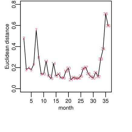
(a)

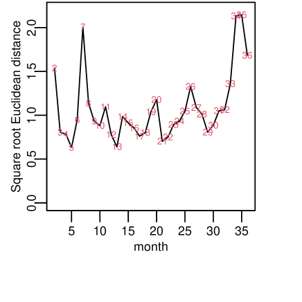
(b)

Figure 1: Distances, $d(\mathbf{L}_{i-1},\mathbf{L}_{i}),i=2,\ldots,36$, between consecutive observations for the monthly Enron networks for (a) the Euclidean metric, $d_{1}$, and (b) the square root Euclidean metric, $d_{\frac{1}{2}}$.

In Figure 1 we plot the distances between consecutive monthly graph Laplacians using Euclidean distance (a) and square root Euclidean distance (b). Some of the largest successive distances are at times $1-2,6-7,33-34,34-35,35-36$, and these are possible candidate positions for anomalous networks that are rather different.

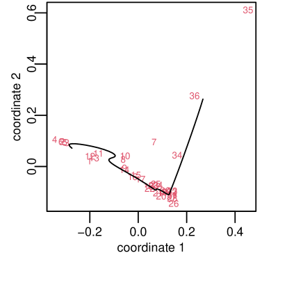
(a)

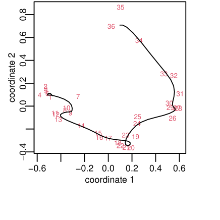
(b)

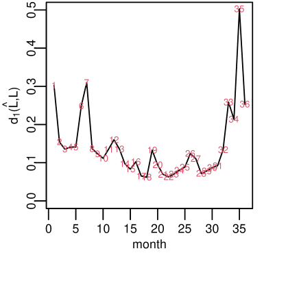
(c)

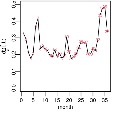
(d)

Figure 2: PCA plots showing the data and Nadaraya-Watson curves, and residual plots for the Enron network data. In each plot the red digits indicate the observation number (month index). In the upper plots the black lines show the Nadaraya-Watson regression curves in the space of the first two principal components, using (a) the Euclidean metric, $d_{1}$, and $h=2$; (b) the Square root Euclidean metric, $d_{\frac{1}{2}}$, and $h=1$. We performed the calculations for a various values $h=0.5,1,2,4,8$, and the chosen value of $h$ was whichever that was optimal with respect to (14). Plots (c) and (d) are corresponding residual plots showing distance $d(\hat{\mathbf{L}}_{i},{\mathbf{L}}_{i})$ between the fitted values $\hat{\mathbf{L}}_{i}$ and the observations ${\mathbf{L}}_{i}$.

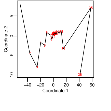
(a)

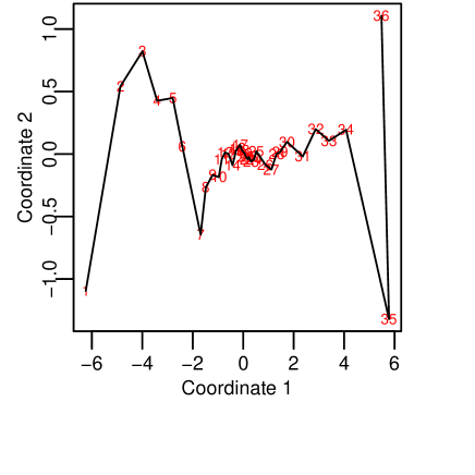
(b)

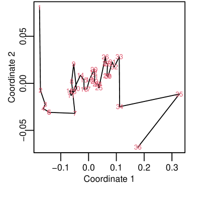
(c)

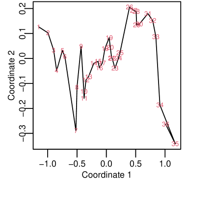
(d)

Figure 3: The red digits indicate the month of the data. MDS plots using the Mahalanobis metric for (a) the Enron data with $\alpha=1$ and (b) with $\alpha=\frac{1}{2}$ using an overall estimate from $\rho$, and the Mahalanobis metric when $\rho$ is estimated to maximize the variance explained by PC1 for (c) the Enron data with $\alpha=1$ and (d) with $\alpha=\frac{1}{2}$.

We provide a PCA plot of the first two PC scores in Figure 2(a),(b) and include the Nadaraya-Watson estimator projected into the space of the first two PCs. Here the bandwidth has been chosen by cross-validation as $h=2$ for the Euclidean case and $h=1$ for the square root metric. The Nadaraya-Watson estimator provides a smooth path through the data, and the structure is clearer in the square root metric plot.

We are interested in finding anomalies in the Enron dynamic networks and so we compute the distances from each network to the fitted value from the Nadaraya-Watson estimate. Figure 2 shows these residual distances of each graph Laplacian to the fitted Nadaraya-Watson values for (c) the Euclidean metric and (d) the square root metric. Some of the largest residuals are months 1,7,35 for Euclidean and 7,33,34,35 for the square root metric, and these are candidates for anomalies.

From Figure 2(b) it looks like there is an approximate horseshoe shape in the PC score plot which could be an example of the horseshoe effect (Kendall,, 1971; Diaconis et al.,, 2008; Morton et al.,, 2017). We might conclude there is a change point in the data around months 20-26 from these plots but this may be misleading (Kendall,, 1970). Explained in Mardia et al., (1979, page 412), the horseshoe effect occurs when the distances which are “large”, between data points, appear the same as those that are “moderate”. Morton et al., (2017) described this as a “saturation property” of the metric, and so on the PCA plot the point corresponding to a ‘large’ time is pulled in closer to time 1 than we intuitively would expect.

As an alternative to PCA, which seeks to address this horseshoe effect, we consider multidimensional scaling (MDS) with a Mahalanobis metric in the tangent space (Mardia et al.,, 1979, p.31) between two graph Laplacians $\mathbf{L}_{k}$ and $\mathbf{L}_{l}$, at times $k$ and $l$ respectively, which is:

$$\sqrt{(\pi_{0}^{-1}(\text{F}_{\alpha}(\mathbf{L}_{k}))-\pi_{0}^{-1}(\text{F}_{\alpha}(\mathbf{L}_{l}))-\boldsymbol{\mu})^{T}\boldsymbol{\Sigma}_{kl}^{-1}(\pi_{0}^{-1}(\text{F}_{\alpha}(\mathbf{L}_{k}))-\pi_{0}^{-1}(\text{F}_{\alpha}(\mathbf{L}_{l}))-\boldsymbol{\mu})},$$

where $\boldsymbol{\mu}$ and $\boldsymbol{\Sigma}_{kl}$ are the mean and covariance matrix of $\pi_{0}^{-1}(\text{F}_{\alpha}(\mathbf{L}_{k}))-\pi_{0}^{-1}(\text{F}_{\alpha}(\mathbf{L}_{l}))$ respectively. Here we take $\boldsymbol{\mu}$ as zero and consider an isotropic AR(1) model which has covariance matrix

$$\boldsymbol{\Sigma}_{kl}=\frac{\sigma^{2}\rho^{|k-l|}}{1-\rho}\mathbf{I}_{\frac{m(m-1)}{2}},$$

which is a diagonal matrix where the diagonal elements are the variance of elements and we have assumed a 0 covariance between any other elements. Writing $\mathbf{y}_{k}=\pi_{0}^{-1}(\text{F}_{\alpha}(\mathbf{L}_{k}))$ and $\mathbf{v}_{k}=\pi_{0}^{-1}(\text{F}_{\alpha}(\mathbf{L}_{k-1}))$ we estimate $\rho$ by least squares $\rho=\frac{\sum_{k=2}^{n}(\mathbf{y}_{k}^{T}\mathbf{v}_{k})}{\sum_{k=2}^{n}(\mathbf{v}_{k}^{T}\mathbf{v}_{k})},$ and we take $\sigma=1$ as this is just an overall scale parameter. The Mahalanobis metric between graph Laplacians, $\mathbf{L}_{k}$ and $\mathbf{L}_{l}$, can now be written as

$$=\sqrt{\frac{1-\rho}{\rho^{|k-l|}}(\pi_{0}^{-1}((\text{F}_{\alpha}(\mathbf{L}_{k}))-\pi_{0}^{-1}(\text{F}_{\alpha}(\mathbf{L}_{l})))^{T}(\pi_{0}^{-1}(\text{F}_{\alpha}(\mathbf{L}_{k}))-\pi_{0}^{-1}(\text{F}_{\alpha}(\mathbf{L}_{l})))}$$

$$=\sqrt{\frac{1-\rho}{\rho^{|k-l|}}}\|\pi_{0}^{-1}(\text{F}_{\alpha}(\mathbf{L}_{k}))-\pi_{0}^{-1}(\text{F}_{\alpha}(\mathbf{L}_{l}))\|=\sqrt{\frac{1-\rho}{\rho^{|k-l|}}}\|\text{F}_{\alpha}(\mathbf{L}_{k})-\text{F}_{\alpha}(\mathbf{L}_{l})\|=\sqrt{\frac{1-\rho}{\rho^{|k-l|}}}d_{\alpha}(\mathbf{L}_{k},\mathbf{L}_{l}).$$

The plot of MDS with the Mahalanobis distance are given in Figure 3(a)-(b). In both plots there are large distances between the first few and last few observations compared to the central observations, which is broadly in keeping with Figure 1(a),(b) although the middle observations do seem too close together in the MDS plots. We consider an alternative estimate in choosing $\rho$ that maximises the variance explained by the first PC scores for each example, shown in Figure 3(c)-(d). These final MDS plots are more in agreement with the distance plots of Figure 1. In particular in Figure 3(d) we see that months 7, 34, 35, 36 look rather different from the rest.

Finally we consider the main features of all the results from Figure 1-Figure 3 and we see that the 7th, 34th and 35th months stand out as strong anomalies. The 7th month corresponds to December 1999, and this is picked out to be an anomaly in Wang et al., (2014), believed to coincide with Enron’s tentative sham energy deal with Merrill Lynch created to meet profit expectations and boost the stock price. Month 34 and 35 correspond to March and April 2002 these correspond to the former Enron auditor, Arthur Andersen, being indicted for obstruction of justice (The Guardian,, 2006).

4 Application: 19th century novel networks

We consider an application where it is of interest to analyze dynamic networks from the novels of Jane Austen and Charles Dickens. The 7 novels of Austen and 16 novels of Dickens were represented as samples of network data by Severn et al., (2020). Each novel is represented by a network where each node of the network is a word, and edges are formed with weights proportional to the number of times a pair of words co-occurs closely in the text. For each novel we produce a network counting pairwise word co-occurrences, and words are said to co-occur if they appear within five words of each other in the text. A choice that needs to be made is if we allow co-occurrences over sentence boundaries and chapter boundaries (Evert,, 2008, Section 3), and for this dataset we allow it. The data are obtained from CLiC (Mahlberg et al.,, 2016).

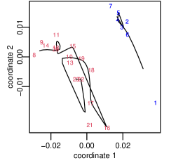
(a)

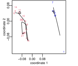
(b)

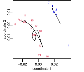
(c)

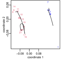
(d)

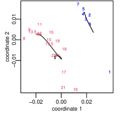
(e)

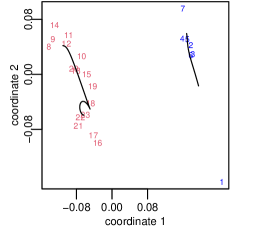
(f)

Figure 4: Regression paths for Austen novels (blue) between the years 1794 to 1815, numbered 1-7 according to chronology of the novels, and for Dickens novels (red) between the years 1836 to 1870, numbered 8-23; using (left to right) $d=d_{1}$ and $d=d_{\frac{1}{2}}$, with bandwidth (top to bottom) $h=1,\,2,\,4$, of which $h=4$ gave the smallest value of the cross-validation criterion (14).

We take the node set $V$ as the $m=1000$ most common words across all the novels of Austen and Dickens. A pre-processing step for the novels is to normalise each graph Laplacian, in order to remove the gross effects of different lengths of the novels, by dividing each graph Laplacian by its own trace, resulting in a trace of 1 for each novel. Our key statistical goal is to investigate the authors’ evolving writing styles, by carrying out non-parametric regression with a graph Laplacian response on the year $t$ that each novel was written.

We apply the Nadaraya-Watson regression to the Jane Austen and Charles Dickens networks separately to predict their writing styles at different times. The response is a graph Laplacian and the covariate is time $t$ for each novel, with a separate regression for each novelist. We compared using the metrics $d_{1}$ and $d_{\frac{1}{2}}$. For each author a Nadaraya-Watson estimate was produced for every 6 months within the period the author was writing. We compared different bandwidths, $h$, in the Gaussian kernel. The results are shown in Figure 4 plotted on the first and second principal component space for all the novels.

For both metrics for Dickens when $h=1$ the regression lines are not at all smooth. For both metrics with $h=2$ the regression line for Dickens appears to show an initial smooth trend, then a turning point around the years 1850 and 1851 (between David Copperfield and Bleak House which are novels 16 and 17 in Figure 4). After 1851 there is much less dependence on time. This change in structure is especially evident in the $h=4$ plot for both metrics, which has the smallest value of the cross-validation criterion (14) out of these choices $h\in\{1,2,4\}$. In the year 1851 Dickens had a tragic year including his wife having a nervous breakdown, his father dying and his youngest child dying (Charles Dickens Info,, 2020). We see that the possible turning point is around the same time as these significant events.

As there are far fewer novels written by Austen it is less obvious if there is any turning point in her writing, however it is clear that Lady Susan (novel 1) is an anomaly, not fitting with the regression curve that does follow Austen’s other works more closely. Lady Susan is Austen’s earliest work, and is a short novella published 54 years after Austen’s death.

5 Discussion

The two applications presented involve a scalar covariate, but the Nadaraya-Watson estimator is appropriate to more general covariates, e.g. spatial covariates. A further extension would be to adapt the method of kriging, also referred to as Gaussian process prediction. Kriging is a geospatial method for prediction at points on a random field (e.g. see Cressie,, 1993), and Pigoli et al., (2016) considered kriging for manifold-valued data. The kriging predictor of an unknown graph Laplacian $\mathbf{L}(\mathbf{x})$ on a random field with known coordinates $\mathbf{x}$ for the dataset $(\{\mathbf{L}_{1},\mathbf{x}_{1}\},\dots,\{\mathbf{L}_{n},\mathbf{x}_{n}\})$ is of the form $Z(\mathbf{x})=\sum_{i=1}^{n}b(\mathbf{x}_{i})\mathbf{L}_{i}$, where the weights, $b(\mathbf{x}_{i})$, are determined by minimizing the mean square prediction error for a given covariance function.

The Nadaraya-Watson estimator can also be applied in a reverse setting where some variable $\mathbf{t}_{i}$ is dependent on the graph Laplacian $\mathbf{L}_{i}$, this can be written as $\mathbf{t}_{i}=\mathbf{t}(\mathbf{L}_{i})$. This could be used if, for example, one had the times networks were produced and then wanted to predict the time a new network was produced. In this case the Nadaraya-Watson estimator is a linear combination of known $\mathbf{t}_{i}$ values, weighted by the graph Laplacian distances, given by

$$\hat{\mathbf{t}}(\mathbf{L})=\frac{\sum_{i=1}^{n}K_{h}(d(\mathbf{L},\mathbf{L}_{i}))\mathbf{t}_{i}}{\sum_{i=1}^{n}K_{h}(d(\mathbf{L},\mathbf{L}_{i}))},$$ (15)

where $d$ can be any metric between two graph Laplacians. Severn, (2019) provided an application of this approach using the Gaussian kernel defined in (7), predicting the time that a novel was written using the network graph Laplacian as a covariate.

Other metrics could also be used, for example the Procrustes metric of Severn et al., (2020). To solve (9) for the Procrustes metric, the algorithm for obtaining a weighted generalised Procrustes mean given in Dryden and Mardia, (2016, Chapter 7) can be implemented.

In Euclidean space there are more general results for the Nadaraya-Watson estimator including weak convergence in $L_{p}$ norm, rather than $p=2$ results that we have used (Devroye and Wagner,, 1980; Spiegelman and Sacks,, 1980). More general results also exist, e.g. see Walk, (2002), including strong consistency. It will be interesting to explore which of these results can be extended to graph Laplacians, although the additive properties of the $p=2$ case have been particularly important in our work.

References

- Charles Dickens Info, (2020) Charles Dickens Info (2020). Charles Dickens timeline. Perry Internet Consulting. https://www.charlesdickensinfo.com/life/timeline/ Last accessed on 2020-09-29.
- Cressie, (1993) Cressie, N. A. C. (1993). Statistics for Spatial Data, Revised Edition. Wiley, New York.
- Devroye and Wagner, (1980) Devroye, L. P. and Wagner, T. J. (1980). Distribution-free consistency results in nonparametric discrimination and regression function estimation. Ann. Statist., 8(2):231–239.
- Diaconis et al., (2008) Diaconis, P., Goel, S., and Holmes, S. (2008). Horseshoes in multidimensional scaling and local kernel methods. The Annals of Applied Statistics, 2(3):777–807.
- Diesner et al., (2005) Diesner, J., Frantz, T. L., and Carley, K. M. (2005). Communication networks from the Enron email corpus “it’s always about the people. Enron is no different”. Computational & Mathematical Organization Theory, 11(3):201–228.
- Dryden et al., (2009) Dryden, I. L., Koloydenko, A., and Zhou, D. (2009). Non-Euclidean statistics for covariance matrices, with applications to diffusion tensor imaging. Ann. Appl. Stat., 3(3):1102–1123.
- Dryden and Mardia, (2016) Dryden, I. L. and Mardia, K. V. (2016). Statistical shape analysis with applications in R. Wiley Series in Probability and Statistics. John Wiley & Sons, Ltd., Chichester, second edition.
- Dubey and Mueller, (2019) Dubey, P. and Mueller, H.-G. (2019). Functional models for time-varying random objects. Journal of the Royal Statistical Society, Series B. to appear.
- Efron and Tibshirani, (1993) Efron, B. and Tibshirani, R. (1993). An Introduction to the Bootstrap. Chapman and Hall, London.
- Evert, (2008) Evert, S. (2008). Corpora and collocations. Corpus linguistics. An international handbook, 2:1212–1248.
- Friel et al., (2016) Friel, N., Rastelli, R., Wyse, J., and Raftery, A. E. (2016). Interlocking directorates in Irish companies using a latent space model for bipartite networks. Proceedings of the National Academy of Sciences, 113(24):6629–6634.
- Ginestet et al., (2017) Ginestet, C. E., Li, J., Balachandran, P., Rosenberg, S., Kolaczyk, E. D., et al. (2017). Hypothesis testing for network data in functional neuroimaging. The Annals of Applied Statistics, 11(2):725–750.
- Guo and Srivastava, (2020) Guo, X. and Srivastava, A. (2020). Representations, metrics and statistics for shape analysis of elastic graphs. In 2020 IEEE/CVF Conference on Computer Vision and Pattern Recognition Workshops (CVPRW), pages 3629–3638, Los Alamitos, CA, USA. IEEE Computer Society.
- Kang et al., (2017) Kang, X., Ganguly, A., and Kolaczyk, E. D. (2017). Dynamic networks with multi-scale temporal structure. In 51st Asilomar Conference on Signals, Systems, and Computers (ACSSC 2017). IEEE Signal Processing Society.
- Kendall, (1970) Kendall, D. G. (1970). A mathematical approach to seriation. Philosophical Transactions of the Royal Society of London. Series A, Mathematical and Physical Sciences, 269(1193):125–134.
- Kendall, (1971) Kendall, D. G. (1971). Abundance matrices and seriation in archaeology. Probability Theory and Related Fields, 17(2):104–112.
- Klimt and Yang, (2004) Klimt, B. and Yang, Y. (2004). Introducing the Enron corpus. In Proceedings of the Conference on Email and Anti-Spam, Mountain View, CA.
- Kolaczyk, (2009) Kolaczyk, E. D. (2009). Statistical analysis of network data: methods and models. Springer Science & Business Media.
- Mahlberg et al., (2016) Mahlberg, M., Stockwell, P., de Joode, J., Smith, C., and O’Donnell, M. B. (2016). CLiC Dickens: novel uses of concordances for the integration of corpus stylistics and cognitive poetics. Corpora, 11(3):433–463.
- Mardia et al., (1979) Mardia, K. V., Kent, J. T., and Bibby, J. M. (1979). Multivariate Analysis. Academic Press, London.
- Marron and Alonso, (2014) Marron, J. S. and Alonso, A. M. (2014). Overview of object oriented data analysis. Biometrical Journal, 56(5):732–753.
- Morton et al., (2017) Morton, J. T., Toran, L., Edlund, A., Metcalf, J. L., Lauber, C., and Knight, R. (2017). Uncovering the horseshoe effect in microbial analyses. MSystems, 2(1):e00166–16.
- Nadaraya, (1965) Nadaraya, É. (1965). On non-parametric estimates of density functions and regression curves. Theory of Probability & Its Applications, 10(1):186–190.
- Pigoli et al., (2014) Pigoli, D., Aston, J. A. D., Dryden, I. L., and Secchi, P. (2014). Distances and inference for covariance operators. Biometrika, 101(2):409–422.
- Pigoli et al., (2016) Pigoli, D., Menafoglio, A., and Secchi, P. (2016). Kriging prediction for manifold-valued random fields. Journal of Multivariate Analysis, 145:117 – 131.
- Rastelli et al., (2018) Rastelli, R., Latouche, P., and Friel, N. (2018). Choosing the number of groups in a latent stochastic block model for dynamic networks. Network Science, 6(4):469–493.
- Rossi and Ahmed, (2015) Rossi, R. A. and Ahmed, N. K. (2015). The network data repository with interactive graph analytics and visualization. In AAAI. http://networkrepository.com.
- Severn, (2019) Severn, K. E. (2019). Manifold-valued data analysis of networks and shapes. PhD thesis, University of Nottingham.
- Severn et al., (2020) Severn, K. E., Dryden, I. L., and Preston, S. P. (2020). Manifold valued data analysis of samples of networks, with applications in corpus linguistics. arXiv e-prints, page arXiv:1902.08290.
- Shetty and Adibi, (2004) Shetty, J. and Adibi, J. (2004). The Enron email dataset database schema and brief statistical report. Information sciences institute technical report, University of Southern California, 4(1):120–128.
- Spiegelman and Sacks, (1980) Spiegelman, C. and Sacks, J. (1980). Consistent window estimation in nonparametric regression. Ann. Statist., 8(2):240–246.
-
The Guardian, (2006)
The Guardian (2006).
Timeline: Enron. Date of article: January 30th, 2006.
https://www.theguardian.com/business/2006/jan/30/corporatefraud.enron
Last accessed on 2020-09-29. - Walk, (2002) Walk, H. (2002). Almost sure convergence properties of Nadaraya-Watson regression estimates. In Dror, M., L’Ecuyer, P., and Szidarovszky, F., editors, Modeling Uncertainty: An Examination of Stochastic Theory, Methods, and Applications, pages 201–223, New York, NY. Springer US.
- Wang et al., (2014) Wang, H., Tang, M., Park, Y., and Priebe, C. E. (2014). Locality statistics for anomaly detection in time series of graphs. IEEE Transactions on Signal Processing, 62(3):703–717.
- Watson, (1964) Watson, G. S. (1964). Smooth regression analysis. Sankhya: The Indian Journal of Statistics, Series A (1961-2002), 26(4):359–372.