Asymptotic state transformations of continuous variable resources
Abstract
We study asymptotic state transformations in continuous variable quantum resource theories. In particular, we prove that monotones displaying lower semicontinuity and strong superadditivity can be used to bound asymptotic transformation rates in these settings. This removes the need for asymptotic continuity, which cannot be defined in the traditional sense for infinite-dimensional systems. We consider three applications, to the resource theories of (I) optical nonclassicality, (II) entanglement, and (III) quantum thermodynamics. In cases (II) and (III), the employed monotones are the (infinite-dimensional) squashed entanglement and the free energy, respectively. For case (I), we consider the measured relative entropy of nonclassicality and prove it to be lower semicontinuous and strongly superadditive. One of our main technical contributions, and a key tool to establish these results, is a handy variational expression for the measured relative entropy of nonclassicality. Our technique then yields computable upper bounds on asymptotic transformation rates, including those achievable under linear optical elements. We also prove a number of results which guarantee that the measured relative entropy of nonclassicality is bounded on any physically meaningful state and easily computable for some classes of states of interest, e.g., Fock diagonal states. We conclude by applying our findings to the problem of cat state manipulation and noisy Fock state purification.
I Introduction
In recent years, the paradigm of quantum resource theories has established itself as the main framework to analyze and assess the operational usefulness of quantum resources Bennett (2004); Coecke et al. (2016); Chitambar and Gour (2019). The general setting involves two sets of objects that are considered easily accessible: free states and free operations. Once these have been identified, the resource content of a state is determined by its transformation properties under free operations (Chitambar and Gour, 2019, Section V). In the long-established tradition of classical Shannon (1948); Cover and Thomas (2006) as well as quantum Bennett et al. (1996a); Plenio and Virmani (2007); Horodecki et al. (2009) information theory, in this work we consider ultimate limitations on those transformation properties, and thus look at the asymptotic setting. Namely, we study free approximate conversion of a large number of copies of the initial state into as many copies of the target state as possible, under the constraint that the approximation error vanishes asymptotically. The resulting transformation rate can be turned into a whole family of resource quantifiers: for a fixed resourceful state (respectively, ), the function (respectively, ) is a resource quantifier with a solid operational interpretation. In entanglement theory, for example, considering free all those transformations that can be implemented with local operations assisted by classical communication (LOCC) and choosing as fixed states Bell pairs, the above procedure leads to the distillable entanglement and the entanglement cost, respectively (Horodecki et al., 2009, Section XV).
Since exact computations of asymptotic transformation rates are often challenging, it is important to establish rigorous bounds on them. In finite-dimensional resource theories, it is possible do so as follows: if is a resource monotone, i.e., a function from quantum states to the set of nonnegative real numbers that does not increase under free operations, the inequality holds if is (i) additive on multiple copies of a state, and (ii) asymptotically continuous Vidal (2000); Horodecki et al. (2000); Donald et al. (2002); Horodecki (2001); Synak-Radtke and Horodecki (2006) (see also (Chitambar and Gour, 2019, Section VI.A.5)). Property (i) can be enforced by regularization (Chitambar and Gour, 2019, Section VI.A.4), and (ii) turns out to hold for many monotones in finite-dimensional systems. For infinite-dimensional resource theories, this approach is however not viable, because the conventional definition of asymptotic continuity, which involves the dimension of the underlying Hilbert space, becomes meaningless. And indeed, in infinite dimensions many monotones — especially those based on entropic quantities — are discontinuous everywhere Wehrl (1976, 1978); Eisert et al. (2002). A weaker version of asymptotic continuity can be restored by imposing an energy constraint Shirokov (2018, 2020a, 2020b); Eisert et al. (2002), yet doing so still does not result in any bound on the transformation rates, because the free operations employed are a priori not required to be (uniformly) energy-constrained. Due to this seemingly merely technical complication, we are not aware of any general technique to upper bound asymptotic transformation rates in infinite-dimensional quantum resource theories prior to our work. We dub this state of affairs the “asymptotic continuity catastrophe”.
This situation is particularly undesirable because infinite-dimensional systems, especially quantum harmonic oscillators, are ubiquitous in physics, and — as suggested by quantum field theory — perhaps fundamental. The optical modes that underlie the flourishing field of continuous variable (CV) quantum technologies Braunstein and van Loock (2005); Cerf et al. (2007); Weedbrook et al. (2012) are a prime example, but harmonic oscillators appear whenever the behavior of a physical system close to equilibrium is approximated to second order.
Here, we devise a simple yet general way to circumvent the asymptotic continuity catastrophe, and establish rigorous bounds on transformation rates that are equally valid for finite- and infinite-dimensional quantum resource theories. Our approach relies on monotones that satisfy, in addition to (i), also (ii’) lower semicontinuity, which is much weaker than (ii) and does not depend upon the Hilbert space dimension, and (iii) strong superaddivity, i.e., . We show how (i), (ii’), and (iii) combined imply the sought general bound on the transformation rate (Theorem 15).
We then study three main applications, to the infinite-dimensional resource theories of: (I) optical nonclassicality Sperling and Vogel (2015); Tan et al. (2017); Yadin et al. (2018); Tan and Jeong (2019); Lami et al. (2021); Regula et al. (2021); (II) quantum entanglement Bennett et al. (1996a); Plenio and Virmani (2007); Horodecki et al. (2009); and (III) continuous variable quantum thermodynamics Brandão et al. (2013); Goold et al. (2016). Each of these applications rests upon a different strongly superadditive monotone, namely (I) the measured relative entropy of nonclassicality, introduced and studied here, (II) the squashed entanglement Tucci (1999); Christandl and Winter (2004); Brandão et al. (2011); Li and Winter (2014); Shirokov (2016a), and (III) the free energy Brandão et al. (2013). Albeit strong subadditivity was known to hold for the latter two monotones, it is only thanks to our Theorem 15 that we are able to employ this mathematical property to deduce an upper bound on asymptotic transformation rates. To the extent of our knowledge, ours are the first such bounds for any and thus in particular the above infinite-dimensional resource theories.
From the technical standpoint, our main results are obtained in the context of nonclassicality (I). Here, one of our key contributions is the proof of a handy variational expression for the measured relative entropy of nonclassicality. This result relies on a careful application of Sion’s Theorem, based, in turn, on a crucial and carefully made choice of topology on the space of trace class operators acting on an infinite-dimensional Hilbert space. This variational expression has several implications, most notably: (a) it immediately implies strong superadditivity, allowing us to deduce (b) the sought bound on asymptotic transformation rates; and finally (c) it points to a technique for estimating, up to arbitrary precision, said upper bound. Another useful result established here is the finiteness of our nonclassicality monotones for any state with either finite energy or finite Wehrl entropy. Other nonclassicality monotones, such as the standard robustness of nonclassicality Lami et al. (2021); Regula et al. (2021), often diverge, giving little to no information about the actual resource content of a state.
This manuscript is organized as follows. In Section II we introduce the basic notation and concepts of quantum mechanics for infinite-dimensional systems that will be used in the remainder of the work. Then, Section III features a concise review of the mathematical framework of quantum resource theories. In Section IV we introduce our main results, in particular Theorems 15, 19, and 23, and briefly discuss their implications. The proofs start from Section V, where we initiate the study of our monotones. In Section VI we establish our first main result, Theorem 15, together with some of its consequences. Section VII is devoted instead to the more involved proof of Theorems 19 and 23. In Section VIII we explore further properties of our nonclassicality monotones. In the subsequent Section IX we apply them to study a wealth of examples, including noisy Fock states, Schrödinger cat states, and squeezed states; we also test our bounds on rates for the case of distillation and dilution of Fock states and cat states in the theory of nonclassicality. Appendix A is concerned with various restricted notions of asymptotic continuity for infinite-dimensional systems and with their limitations in proving general bounds on asymptotic transformation rates, which further motivates our analysis.
II Quantum mechanics for infinite-dimensional systems
With every quantum system one associates a Hilbert space ; in this work we will be mainly concerned with the case where , i.e., with infinite-dimensional quantum systems. When dealing with (both finite- and infinite-dimensional) open quantum systems, both physical states and observables are described in terms of linear self-adjoint operators acting on and fulfilling specific properties. As we will discuss in a moment, the structure of operator spaces is more complex in the infinite-dimensional case than in the finite-dimensional one, where many of them coincide. We start by setting the basic notation and definitions and introduce the objects that we will use in the following.
II.1 Notation and definitions
For a generic linear self-adjoint operator acting on a Hilbert space one can define the operator norm as follows:
Operators with finite operator norm, i.e., are said to be bounded. Moreover, an operator is said to be trace class if its trace norm
is finite, where is any orthogonal basis of . For trace class operators we can define the trace as:
which is independent of the choice of the orthogonal basis . The trace norm of a trace class operator can then be written as .
We are now ready to list below the most relevant operator spaces:
-
•
: the Banach space of bounded self-adjoint operators on ;
-
•
: the Banach space of self-adjoint trace class operators on ;
-
•
: the Banach space of self-adjoint compact operators on , defined as the closure with respect to the operator norm of ;
-
•
: the set of density operators (i.e., positive semidefinite trace class operators with trace ) on ;
-
•
: the cone of positive semidefinite (and hence self-adjoint) trace class operators on ;
-
•
: the cone of positive semidefinite (and hence self-adjoint) compact operators on ;
One has that , with equality iff is finite dimensional. Also, the duality relation holds at the level of Banach spaces. We remind the reader that the dual of a Banach space equipped with a norm is the vector space of all linear functionals such that , equipped with the norm .
A quantum state on a quantum system with Hilbert space is represented by a density operator . Quantum channels from to , where are quantum systems, are completely positive trace preserving maps . For a quantum channel , the adjoint is the linear map defined by for all and . Among the simplest examples of quantum channels are quantum measurements, represented by positive operator-valued measures (POVM), i.e., finite collections of positive semidefinite (bounded) operators that obey the normalization rule . Any quantum measurement can be written as a trace-preserving map by making use of classical flags : , where is the output state in case the outcome is measured.
It is well known that the topological structure of infinite-dimensional spaces is much richer than in the finite-dimensional case. There is a wealth of topologies that can be defined on infinite-dimensional Banach spaces, and in particular on the operator spaces discussed above Wikipedia contributors (2017). In light of this fact, and for later convenience, we provide here a quick guide:
-
•
the weak operator topology on (and hence on and ) is the coarsest topology that makes all functionals continuous, for all ;
-
•
the weak* topology on is the coarsest topology that makes all functionals continuous, for all ;
-
•
the weak topology on is the coarsest topology that makes all functionals continuous, for all ;
-
•
the trace norm topology on is the one induced by the trace norm ;
-
•
the operator norm topology on is the one induced by the operator norm .
The role of the weak* topology on will play a special role for us (cf. Lemma 38).
Remark 1.
The weak* topology is the topology induced by the Banach space on its dual . Therefore, by the Banach–Alaoglu theorem the unit ball of is weak* compact. This fact will be crucial for one of the main results of the work.
We conclude this section by stating some useful facts about operator topologies. We start by noting the following remarkable lemma, originally discovered by Davies (Davies, 1969, Lemma 4.3) — see also the ‘gentle measurement lemma’ by Winter (Winter, 1999, Lemma 9) for a refined version.
Lemma 2 ((Davies, 1969, Lemma 4.3)).
For a net111A net on some set is any function of the form , where is a directed set, i.e., a set equipped with a preorder such that for all there exists with the property that and . of positive semidefinite trace class operators, if in the weak operator topology, and moreover , then in norm.
Since two topologies are equal if and only if they have the same convergent nets, it is immediate to deduce the following.
Corollary 3.
The weak topology and the norm topology coincide on . They also coincide with the weak operator topology on .
Remark 4.
The norm topology does not coincide with the weak operator topology on . For instance, the sequence of Fock states converges to in the weak operator topology, but it is not convergent in the norm topology (for instance because it is not of Cauchy type).
II.2 Continuous variable systems
Among all infinite-dimensional quantum systems, a central role is played by continuous variable (CV) systems, and here, perhaps most notably, by finite collections of harmonic oscillators. The Hilbert space corresponding to an -mode CV system is composed of all square-integrable complex-valued functions on the Euclidean space , denoted with ; one can then identify . Note that we will adopt the convention hereafter. Then, the canonical operators and () satisfy the canonical commutation relations and , with denoting the identity over . It is customary to define the annihilation and creation operators by
| (1) |
In terms of , the canonical commutation relations take the form , .
On a single-mode system, Fock states are defined for by , where is the vacuum state. For , the associated coherent state takes the form Schrödinger (1926); Klauder (1960); Glauber (1963); Sudarshan (1963)
| (2) |
Extending these definitions to multimode systems is quite straightforward. For , one sets ; analogously, for , a multimode coherent state is defined by .
The displacement operators form a special family of unitary operators acting on . For , they are defined by
| (3) |
They satisfy the identity
| (4) |
called the Weyl form of the canonical commutation relations, for all , and they yield coherent states upon acting on the vacuum, i.e.,
| (5) |
For an arbitrary trace class operator , its characteristic function is given by
| (6) |
For a -mode quantum state , a quantity which is intimately related to its characteristic function is the Husimi -function , defined by Husimi (1940).
II.3 Entropies and relative entropies
The (von Neumann) entropy of some positive semidefinite trace class operator can be defined as
| (7) |
Note that this is a well-defined although possibly infinite quantity. One way to make sense of the expression (7) is via the infinite sum , where is the spectral decomposition of where we convene that . Since because is trace class, the terms of the above sum are eventually positive. Hence, the sum itself can be assigned a well-defined value, possibly . An alternative approach is to define is the Wehrl entropy instead:
| (8) |
It is well known that for any quantum state .
The relative entropy between two positive is usually written as Umegaki (1962); Ohya and Petz (2004)
| (9) |
Again, the above expression is well defined and possibly infinite Lindblad (1973). To see why, we represent it as the infinite sum , where and are the spectral decompositions of and , respectively, and we assume that only terms with and are included. As above, we follow the convention of setting , and we set if there exist two indices and with , , and . As detailed in Lindblad (1973), the convexity of implies that all terms of the above infinite sum are non-negative, making the expression well defined. In light of the above discussion, it is not difficult to realize that a necessary condition for to be finite is that . Thus, up to projecting everything onto a subspace we will often assume that is faithful, i.e., that . The relative entropy can be endowed with an operational interpretation in the context of asymmetric hypothesis testing Hiai and Petz (1991); Buscemi et al. (2019); Wang and Wilde (2019).
An alternative approach to the quest for defining a quantum relative entropy could be that of bringing the problem back to the classical setting by means of quantum measurements. Namely, for a state and a measurement , we define the associated outcome probability distribution on as . Remembering that for two classical probability distributions and the Kullback–Leibler divergence is given by Kullback and Leibler (1951), let us define the measured relative entropy between any two states and as Donald (1986); Hiai and Petz (1991)
| (10) |
It is known that for all pairs of states Donald (1986). Recently, extending a result by Petz Petz (1986), Berta et al. have shown that for finite-dimensional systems equality holds if and only if Berta et al. (2017).
III Quantum Resource Theories
In this section we introduce a general notion of quantum resource theory, and some related concepts and results. Note that our definition is slightly different from that in the recent review by Chitambar and Gour (Chitambar and Gour, 2019, Definition 1), in that we require also parallel composition (i.e., tensor product) of free operations to be free.
Definition 5.
A quantum resource theory (QRT) is a pair , where is a family of quantum systems that is closed under tensor products, in the sense that implies that ; and contains the trivial system with Hilbert space , while , called the set of free operations, is a mapping that assigns to every pair of systems a set of channels from system to . Such a set will be denoted with .222Here, classical registers are thought of as special -dimensional quantum systems () with the property that any free operation satisfies that , with being the dephasing map. In other words, if a quantum system plays the role of a classical register, then no state apart from those that are diagonal in a fixed orthonormal basis is ever accessible with free operations. We will require that the following three consistency conditions are satisfied:
-
(i)
for all , the identity is a free operation on , in formula ;
-
(ii)
free operations are closed under sequential compositions, namely, if and , , then also ;
-
(iii)
free operations are closed under parallel compositions, namely, if for one chooses and , then also .
If every system in is finite dimensional, we will say that itself is finite dimensional.
III.1 Monotones
Given a QRT as above, one defines the set of free states on the system as
| (11) |
Clearly, if partial traces are free, then . A central role in our paper is played by resource quantifiers, i.e., monotones. We define them as follows.
Definition 6.
Let be a resource theory. A mapping assigning to each a function on the set of states on that takes on values in the extended reals is called a resource monotone — or simply a monotone — if
-
(i)
holds for all states on and for all free operations , where is arbitrary;
-
(ii)
for all , with defined by (11).
A monotone is said to be:
-
(a)
faithful, if implies that ;
-
(b)
convex, if all functions are convex, i.e., for all and all statistical ensembles on ;
- (c)
-
(d)
lower semicontinuous, if is lower semicontinuous as a function on for all , i.e., if for a sequence of states on implies that ;
-
(e)
strongly superadditive, if holds for all and for all states ;
-
(f)
superadditive, if for all and for all states and ;
-
(g)
weakly superadditive, if for all , for all and all states , where denotes the joint system formed by copies of ;
-
(h)
additive, if for all and for all states and ;
-
(j)
weakly additive, if for all and all states , where denotes the joint system formed by copies of .
Remark 7.
In Definition 6, and .
Remark 8.
Any monotone is automatically invariant under free unitaries whose inverse is also free.
Remark 9.
The notions of upper semicontinuous, strongly subadditive, or subadditive monotone are obtained by reversing the inequalities and exchanging with in (d), (e), and (f) of Definition 6.
Note.
In what follows, with a slight abuse of notation we will often drop the subscript of specifying the system it refers to, and think of a monotone as a function defined directly on the collection of states on all possible systems .
III.2 Transformation rates
We continue by recalling the definition of asymptotic transformation rate.
Definition 10.
Let be a QRT. For any two systems and any two states and , the corresponding (standard) asymptotic transformation rate is given by
| (13) |
where denotes the system composed of copies of . Any number in the set on the right-hand side of (13) is called a (standard) achievable rate for the transformation .
The above definition captures the intuitive notion of maximum yield of copies of the target state that can be obtained per copy of the initial state by means of free operations and with asymptotically vanishing error. In Definition 10, we have measured the error using the global trace distance. However, it is possible and sometimes even reasonable to modify the error criterion. For instance, in a situation where the output copies are distributed to noninteracting parties, what is relevant is the maximum local error rather than the global one. This train of thought inspires the following definition.
Definition 11.
Let be a QRT. For any two systems and any two states and , the corresponding maximal asymptotic transformation rate is given by
| (14) |
where for a state defined on copies of we defined as the reduced state on the subsystem. Any number in the set on the right-hand side of (13) is called a maximally achievable rate for the transformation .
It is immediate to see that for any given pair of states the maximal rate always upper bounds the corresponding standard rate (Lemma 31).
III.3 Infinite-dimensional quantum resource theories
The prime example of a quantum resource theory is naturally that of entanglement Horodecki et al. (2009); Bennett et al. (1996a, b); Chitambar and Gour (2019). In spite of their central importance, very little is known about many fundamental operational questions in the infinite-dimensional case Eisert and Plenio (2003); Eisert et al. (2002); Shirokov (2016b, a), with a partial exception being the theory of Gaussian entanglement Werner and Wolf (2001); Giedke et al. (2001, 2003); Adesso and Illuminati (2007); Lami et al. (2018). We can formally define entanglement as a resource theory as follows.
Definition 12.
The resource theory of bipartite entanglement is defined by setting:
-
•
to be the family of all (possibly infinite-dimensional) quantum systems , where the colon indicates the bipartition in separate parties;
-
•
for any bipartite system , where denotes the closed (in trace norm topology) convex hull of a set;
-
•
is the set of all LOCC protocols from to .
Another important example is the resource theory of quantum thermodynamics Brandão et al. (2013); Narasimhachar et al. (2021); Serafini et al. (2020). Just as that of entanglement, it can be constructed for finite-dimensional systems as well. However, in accordance with the spirit of this work, we will focus on the continuous variable case from now on.
Definition 13.
The resource theory of quantum thermodynamics is defined by setting:
-
•
to be the family of all (possibly infinite-dimensional) quantum systems equipped with a Hamiltonian satisfying the Gibbs hypothesis, i.e., for any inverse temperature ; we also assume for any systems ;
-
•
once an inverse temperature has been fixed for all systems, , with
being the thermal state, for any system with Hamiltonian ;
-
•
to encompass all quantum channels such that for systems with thermal states and respectively (Gibbs-preserving operations).
In the case where the family contains only continuous variable quantum systems, other specific resource theories emerge naturally, as a result of operational or technological constraints. For example, the resource theory of optical nonclassicality Sperling and Vogel (2015); Tan et al. (2017); Yadin et al. (2018); Tan and Jeong (2019); Lami et al. (2021); Regula et al. (2021) is based on the premise that statistical mixtures of coherent states are easy to synthesize, hence free, and “classical”, as they most closely approximate classical electromagnetic waves. On the other hand, operationally, nonclassical states, such as Fock states Knill et al. (2001); Eisaman et al. (2011), squeezed states Kennard (1927); Walls (1983); Slusher et al. (1985); Andersen et al. (2016); Schnabel (2017), cat states Dodonov et al. (1974); Ralph et al. (2003); Lund et al. (2008); Joo et al. (2011); Facon et al. (2016); Brask et al. (2010); Lee and Jeong (2013); Sychev et al. (2017), or NOON states Sanders (1989); Dowling (2008), play an increasingly central role in applications. A formal definition of this resource theory is as follows.
Definition 14.
The resource theory of (optical) nonclassicality is defined by setting:
-
•
to be the family of all continuous variable quantum systems;
-
•
for any -mode system ;
-
•
, with being and -mode systems respectively, to encompass all quantum channels such that (classical operations).
The so-called classical operations comprise, but are possibly not limited to, channels that can be obtained through passive linear optics, destructive measurements, and feed-forward of measurement outcomes Tan et al. (2017); Yadin et al. (2018). Note that the set of classical states and that of classical channels are both convex.
IV Main results
In the present section we state the main results of our work. The starting point is the general bound on asymptotic transformation rates in Theorem 15. We then explore its consequences for the resource theories of entanglement and quantum thermodynamics in Corollaries 16 and 17, respectively. To apply it to the resource theory of nonclassicality, instead, we need to introduce and study two new monotones, the measured relative entropy of nonclassicality and its regularized version (Definition 18). One of our main technical contributions is the proof of a powerful variational expression for (Theorem 19), from which we deduce the lower semicontinuity and — most importantly — the strong superadditivity of the measured relative entropy of nonclassicality (Theorem 23).
IV.1 General bound on asymptotic rates
Our first result is a general bound on (maximal) transformation rates that works for all quantum resource theories, including infinite-dimensional ones. Formally, it is a generalization of a well-known bound holding for many monotones in finite dimensions (Chitambar and Gour, 2019, Section VI.A.5). In this simpler context, it is possible to prove that if a resource monotone is weakly additive and moreover asymptotically continuous (Definition 6, (j) and (c)) then the asymptotic transformation rate between any two states (Definition 10) satisfies that
| (15) |
provided that the right-hand side is well defined. This bound has been proved in (Horodecki, 2001, Theorem 4) (see also (Chitambar and Gour, 2019, Section VI.A.5)) using techniques developed in Horodecki et al. (2000) and Donald et al. (2002) — see especially (Donald et al., 2002, Propositions 19, 20, and 22) for a thorough discussion of many possible variations of the underlying hypotheses. In fact, the proof is so simple and enlightening that it is worth summarising it here. For any achievable rate , i.e., for any element of the set in (13), calling the systems to which pertain, we can construct the sequence of maps such that satisfies . Leveraging properties (j) and (c) in Definition 6, one then obtains that
| (16) |
where we called . Dividing by and taking the limit yields , and in turn (15) once one takes the supremum over .
Inequality (15), applied to different weakly additive and asymptotically continuous monotones, yields many of the commonly employed bounds on rates as far as finite-dimensional resources are concerned.333Notable exceptions are monotones based on the partial transpose in entanglement theory Vidal and Werner (2002); Plenio (2005); Lami and Regula (2021). Unfortunately, for infinite-dimensional systems the notion of asymptotic continuity becomes empty, and consequently the argument in (16) breaks down at the step marked as (c). In fact, prior to our work there seemed to be a lack of technical tools to address the approximation error allowed in the transformation (13) in the infinite-dimensional case. Due to this “asymptotic continuity catastrophe”, in the existing literature prior to our work we could not locate any upper bound on asymptotic transformation rates that holds for infinite-dimensional resource theories. The theorem below, whose proof is remarkably simple (and yet very different from that in (16)) but whose applicability is surprisingly wide, remedies this regrettable state of affairs at least in the case where the employed monotone is strongly superadditive. An alternative but ultimately less satisfactory approach to circumvent the asymptotic continuity catastrophe is sketched out in Appendix A, to which we refer the reader interested in more details on this point.
Theorem 15.
For a given QRT, not necessarily finite dimensional, let be a monotone that is strongly superadditive, weakly additive, and lower semicontinuous. Then, for all states , it holds that
| (17) |
whenever the rightmost side is well defined.
With the above result at hand, we can now establish rigorous bounds on transformation rates in operationally important examples of infinite-dimensional quantum resource theories.
IV.2 First consequences: resource theories of entanglement and quantum thermodynamics
We start with the QRT of entanglement. To the extent of our knowledge, there is no available technique to derive upper bounds on the transformation rate in terms of known monotones. Even the energy-constrained version of asymptotic continuity established by Shirokov Shirokov (2018, 2020a, 2020b) for many entanglement monotones does not suffice to this purpose. This is because we need continuity estimates on the output system, and — while the input, consisting of many copies of a known state, is naturally energy constrained — the output, being produced by a general unconstrained free channel, is not. We could of course impose such an energy constraint artificially, by enforcing the parties to operate with LOCCs that are uniformly energy-constrained; however, the operational motivation behind this assumption is somewhat dubious; this is especially so if energy is much cheaper than entanglement, which is often the case in experimental practice. We refer the reader to Appendix A for a more in-depth discussion of these points.
To apply Theorem 15 to the case at hand, we need an entanglement monotone that obeys strong superadditivity. The squashed entanglement, denoted , is a natural candidate Tucci (1999); Christandl and Winter (2004); Brandão et al. (2011); Li and Winter (2014). Shirokov Shirokov (2016a) has shown how to extend its definition to infinite-dimensional systems (Shirokov, 2016a, Eq. (17)). We report the definition of squashed entanglement later in Section VI.2. Applying Theorem 15 to it we deduce the following corollary.
Corollary 16.
Let and be two bipartite states such that
| (18) |
Then, in the QRT of entanglement it holds that
| (19) |
Another possible application of Theorem 15 is to the QRT of thermodynamics. The quantity , which coincides with the free energy difference between and when , can be seen to be strongly superadditive, additive and lower semicontinuous. We deduce the following.
Corollary 17.
In the QRT of thermodynamics, for all states it holds that
| (20) |
Let us stress that Corollary 17 extends the results of Brandão et al. Brandão et al. (2013), which are valid in finite-dimensional systems, to all quantum systems where a QRT of thermodynamics can be constructed. This is clearly a crucial improvement because of the ubiquity of harmonic oscillators in physical applications.
IV.3 Further consequences: resource theory of nonclassicality
Over the past decades, there have been proposals to quantify the nonclassicality of quantum states of light, e.g., by their distance from the set of classical states Hillery (1987); Dodonov et al. (2000); Marian et al. (2004); Brandão and Plenio (2008), by the amount of noise needed in order to make them classical Lee (1991); Lütkenhaus and Barnett (1995), by their potential for entanglement generation Asbóth et al. (2005); Vogel and Sperling (2014); Killoran et al. (2016) or for metrological advantage Kwon et al. (2019), by the negativity Kenfack and Życzkowski (2004); Tan et al. (2020), the variances Yadin et al. (2018) or other features Vogel (2000a); Diósi (2000); Vogel (2000b); Richter and Vogel (2002); Idel et al. (2016); Bohmann and Agudelo (2020) of their phase-space distributions, or by the minimum number of superposed coherent states needed to reproduce the target state Gehrke et al. (2012). Unfortunately, none of these monotones appears to yield bounds on asymptotic transformation rates, for they fail to satisfy asymptotic continuity. In fact, to the extent of our knowledge, no rigorous bounds on those rates are known for the resource theory of optical nonclassicality. Indeed, the transformations considered in Yadin et al. (Yadin et al., 2018, Theorems 2 and 3) are probabilistic but exact, and moreover single-shot rather than asymptotic. One could argue that especially their zero-error nature somewhat limits their operational relevance in applications.
We therefore pursue a different approach. In analogy to what was previously done for entanglement Vedral et al. (1997); Vedral and Plenio (1998), we use the relative entropies introduced in Section II.3 to construct nonclassicality measures.
Definition 18.
Let be an -mode state. The relative entropy of nonclassicality and the measured relative entropy of nonclassicality of are defined respectively as:
| (21) |
Note that our definition of differs from that of Marian et al. Marian et al. (2004), in that is allowed to be an arbitrary classical state, not necessarily Gaussian. It is not difficult to see that and are faithful and convex nonclassicality monotones (Lemma 28). Since is also subadditive (again, Lemma 28), its regularization is well defined by Fekete’s lemma Fekete (1923) and also subadditive (Corollary 29). We will show that both and are always finite on bounded-energy states (Proposition 30), but that there exist infinite-energy states such that (Proposition 39). Explicit computations or tight estimates for the measured relative entropy of nonclassicality for Fock-diagonal states, squeezed states, and cat states are reported in Sections IX.1–IX.2.
It might not be clear at this point why to introduce alongside with , given that the former quantity involves one more nested optimization than the latter. However, we now show that its computation can be notably simplified.
Theorem 19.
For all -mode finite-entropy states , it holds that
| (22) |
where ranges over all positive trace class operators on (equivalently, on all positive normalized states).
The proof of Theorem 19 involves two main ingredients. This first one is a generalization of the variational program for put forth by Berta et al. (Berta et al., 2017, Lemma 1) to the infinite-dimensional case, which may be of independent interest.
Lemma 20.
Let be a density operators on a (possibly infinite-dimensional) Hilbert space , and let be positive semidefinite and nonzero. Then
| (23) | ||||
| (24) | ||||
| (25) | ||||
| (26) | ||||
| (27) | ||||
| (28) |
The notation in the supremum in equations (25) and (26) means that is required to have eigenvalues bounded from below by a positive quantity, i.e., to satisfy for some , depending on .
Remark 21.
The above Lemma 20 is proved in Section VII.1. By applying it to the program in (21) we are left with a nested optimization of the form . Then, the second critical ingredient that is needed to arrive at a proof of Theorem 19 is an application of Sion’s minimax theorem Sion (1958) that allows us to exchange infimum and supremum in this resulting expression. This is technically challenging, as meeting the compactness hypothesis in Sion’s theorem requires a careful choice of topology on the domain of optimization. The crucial technical contribution here is Lemma 38, which establishes the compactness of the set of subnormalized classical states with respect to the weak*-topology (see Section II.1). Along the way, we introduce and study an auxiliary quantity (Definition 33 and Proposition 35).
An immediate consequence of Theorem 19 is the superadditivity of on finite-entropy states. This fact allows us to successfully construct the regularization .
Corollary 22.
When computed on finite-entropy states, is lower semicontinuous and strongly superadditive, meaning that
| (29) |
Therefore, for any finite-entropy state its regularization
| (30) |
is a well defined nonclassicality monotone. It is lower semicontinuous, strongly superadditive, and weakly additive. Furthermore,
| (31) |
holds whenever . In particular, both and are also faithful, at least on finite-entropy states.
The variational expression in Theorem 19 has many more consequences. For example, we use it to establish upper and lower bounds on and its regularization based on the Wehrl entropy (Proposition 40), which translate to tight estimates of these quantifiers for Gaussian states (Corollary 41). The most important application is however the following.
Theorem 23.
Let be two CV states with finite entropy, i.e., such that . Then the transformation rates in the resource theory of nonclassicality obey the inequalities
| (32) |
provided that the ratios on the right-hand sides are well defined.
To the best of our knowledge, (32) is the first explicit bound on asymptotic transformation rates in the context of CV nonclassicality. However, it would amount to a rather futile theoretical statement if not complemented with a systematic way of upper bounding the ratio . Note that can be estimated from above by simply making suitable ansatzes in (21). The a priori less trivial task of lower bounding can be carried out thanks to Theorem 19.
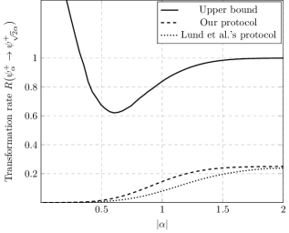
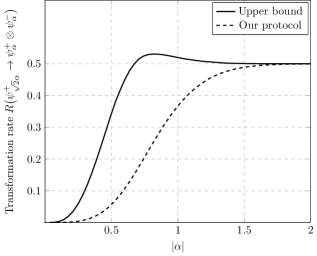
As an immediate application of Theorem 23, we consider the paradigmatic example of (Schrödinger) cat state manipulation Lund et al. (2004); Laghaout et al. (2013); Sychev et al. (2017, 2018); Wang et al. (2018); Oh and Jeong (2018). For , cat states are defined by Dodonov et al. (1974)
| (33) |
where are coherent states (2). The transformations we look at are (amplification) and (sign-randomized dilution). A protocol for amplification using linear optical elements and quadrature measurements has been designed by Lund et al. Lund et al. (2004). We present an ameliorated version of it (Proposition 48), together with a simple protocol for sign-randomized dilution (Proposition 49). The lower bounds on rates given by these explicit protocols are shown in Figure 1. The upper bound derived via Theorem 23 is asymptotically tight for the dilution task, but not in the case of amplification. This is due to the fact that our quantifiers all saturate to for cat states with .
V Preliminary results
Throughout this section we lay the ground for the proof of our main results, studying general properties of monotone regularization (Section V.1) and investigating in more detail nonclassicality monotones (Section V.2).
V.1 Generalities about monotone regularization
It turns out that any monotone can be made weakly additive by a procedure known as “regularization”.
Definition 24.
Let be a QRT equipped with a monotone . Then the functions
| (34) | ||||
| (35) |
are called the lower and upper regularizations of . On the domain of states such that one can speak of a unique regularization .
The following result is immediate from the definition.
Lemma 25.
Let be a QRT equipped with a monotone . Then the lower and upper regularizations and given by Definition 24 are also monotones. Moreover, is weakly additive on its domain, i.e., for a state implies that for all .
Proof.
Let us start by showing that, e.g., is a monotone. Since parallel composition of free operations is free, for all and for all , with , we obtain that
Moreover, if is free, also is so, and hence as well. This proves the first claim.
Now, by definition implies that the sequence has a limit. If that is the case, then clearly for all . ∎
A useful fact that is slightly less obvious is as follows.
Lemma 26.
Let be a QRT equipped with a monotone that is weakly superadditive. Then:
-
(i)
the regularization in Definition 24 exists for all states , i.e., for all with ; it is also weakly additive and satisfies ;
-
(ii)
If is also (strongly) superadditive, then is (strongly) superadditive as well;
-
(iii)
If is lower semicontinuous, then so is .
Remark 27.
The above result is still valid if we replace superadditivity with subadditivity, lower semicontinuity with upper semicontinuity, and reverse all inequalities.
Proof of Lemma 26.
Due to weak superadditivity, for all states the sequence defined by is superadditive, meaning that . Therefore, by Fekete’s lemma Fekete (1923) exists, and it satisfies that . Therefore,
is well defined for all , and satisfies . This proves (i).
Now we proceed to prove points (ii) and (iii). We already saw in Lemma 25 that is a weakly additive monotone, so it suffices to show that it is (strongly) superadditive if was such. This is immediate to establish (we prove it only for strong superadditivity, as the superadditivity case is completely analogous):
To see that is lower semicontinuous if so was , just notice that is the pointwise supremum of lower semicontinuous functions and thus must itself be lower semicontinuous. ∎
V.2 Nonclassicality monotones
If the reader is worried by the proliferation of regularized measures in Definition 18, they should not be. In fact, we will show that the regularizations are unique in all physically interesting cases. We are able to readily prove the equality between and , while a proof for and will be given at the end of Section VII.4. The first step is to prove that the quantity we just defined are actually good resource monotones.
Lemma 28.
The quantities and are faithful and convex nonclassicality monotones. They obey the inequality . Moreover, is subadditive.
Proof.
The argument is completely standard. The inequality is obvious, and follows from the same relation between the relative entropy and its measured version. Since both and obey the data processing inequality, for every classical channel we obtain that
and analogously for . This proves monotonicity.
Convexity descends from the fact that both and are defined as the infimum of a jointly convex function on a convex domain. For example,
The proof for is entirely analogous.
Faithfulness follows, e.g., from Pinsker’s inequality Pinsker (1964), which implies that
where in the last line we used the elementary fact that the trace distance is achieved by the (binary) measurement , with being the projector onto the positive subspace of .
To prove the subadditivity of , just notice that for all -mode CV systems it holds that
where in the third line we used the identity (Ohya and Petz, 2004, Eq. (5.22)). ∎
Corollary 29.
The functions are nonclassicality monotones. The regularization is unique and is a weakly additive nonclassicality monotone; it satisfies that .
We now argue that the monotones behave like useful resource quantifiers on states of physical interest. An essential basic feature is finiteness on bounded-energy states, where the energy is measured by the total photon number Hamiltonian.
Proposition 30.
Let be an -mode state with finite mean photon number . Then
| (36) |
where .
Proof.
It is well known that the entropy of an -mode state with finite mean photon number is at most , which indeed corresponds to the entropy of the thermal state with the same energy. Hence, has finite entropy, so that (31) holds. Thus, we only have to show that . For an arbitrary , let
| (37) |
be the single-mode thermal state of mean photon number . It is well known that , and hence , for all . Therefore,
where we used the variational representation
whose proof is elementary. ∎
Further results on our nonclassicality monotones will be given in Section VIII.
VI Proof of Theorem 15 and of Corollaries 16 and 17
VI.1 Proof of Theorem 15
In this section we prove our first main result, Theorem 15. We start with a simple lemma, which justifies the name of maximal asymptotic transformation rate given to the quantity in Definition 11 (cf. Definition 11).
Lemma 31.
Let be a QRT. For any two systems and any two states and , it holds that
| (38) |
Proof.
For all and all free operations , the data processing inequality for the trace norm Ruskai (1994) implies that
Therefore, a sequence of protocols that achieves a rate in (13) (i.e., that makes the global error vanish) achieves the same rate in (14) (because the maximum local error will also vanish). The claim follows. ∎
We are now ready to present the proof of Theorem 15.
Proof of Theorem 15.
It suffices to show that . For any sequence of free operations satisfying, for all , it holds that
Here, 1 holds due to weak additivity, even without the lim inf and for every ; 2 comes from monotonicity; 3 from strong superadditivity; in 4 we constructed a sequence of indices achieving the minimum; finally, 5 descends from lower semicontinuity and the assumption on . Then a supremum over yields the claim. ∎
Before moving on to the study of the applications, it is perhaps instructive to compare the above argument with the one we saw in (16), where the same bound on rates was proved (under different assumptions) in the finite-dimensional setting. The main difference lies in step 3, in which we exploit strong superadditivity to move the error analysis to the single-copy level, where it is ultimately tackled by means of lower semicontinuity (step 5). In (16), instead, asymptotic continuity was leveraged to carry out an error analysis directly at the many-copy level. This type of ideas had been previously exploited in (Lami, 2020, Theorem 4 and Remark 10).
VI.2 Proof of Corollary 16
We now apply Theorem 15 to the resource theory of entanglement. Let us start by fixing some terminology. The squashed entanglement of a bipartite state of a finite-dimensional bipartite system is defined by Tucci (1999); Christandl and Winter (2004); Brandão et al. (2011); Li and Winter (2014)
| (39) |
where the infimum is over all extensions of the state , i.e., over all tripartite states satisfying that , and
| (40) |
is the conditional mutual information. The problem with the above definition is that it cannot be extended directly to the infinite-dimensional case, because the right-hand side of (40) may contain the undefined expression Shirokov (2016a, b).
Fortunately, Shirokov has found a way out of this impasse. The first step is to construct the conditional mutual information via an alternative expression to (40), namely,
| (41) |
where the supremum is over all finite-dimensional projectors on . An equivalent expression is obtained by exchanging and in (41). Clearly, (41) reduces to (40) when is finite dimensional.
With (41) at hand, (39) can be extended without difficulty to the infinite-dimensional case (Shirokov, 2016a, Eq. (17)). In order for this to work, we have to keep in mind that the system could and in general will be infinite-dimensional.
An alternative strategy to generalize the squashed entanglement to infinite-dimensional systems could be that of truncating the state directly by means of local finite-dimensional projectors. This results in a different function , defined by (Shirokov, 2016a, Eq. (37))
| (42) |
where the infimum runs over all finite-dimensional projectors and . The nested optimizations hidden in (42) make a slightly less desirable quantity than . Nevertheless, we will find it useful in intermediate computations.
The main properties of the two functions and that we will use are as follows:
-
(a)
both and are strongly superadditive (Shirokov, 2016a, Propositions 2B and 3B);
-
(b)
both and are additive, and hence also weakly additive (Shirokov, 2016a, Propositions 2B and 3B);
-
(c)
is lower semicontinuous everywhere (Shirokov, 2016a, Proposition 3A);
-
(d)
on all states with (Shirokov, 2016a, Proposition 3C).
VI.3 Proof of Corollary 17
We now move on to the case of quantum thermodynamics at some (fixed) inverse temperature . The monotone Brandão et al. (2013)
| (43) |
is easily seen to be:
-
(a)
strongly superadditive, because
where the first identity is a consequence of the fact that , while the inequality follows from (Ohya and Petz, 2004, Corollary 5.21);
-
(b)
additive and hence weakly additive, since
finally,
-
(c)
lower semicontinuous, as follows, e.g., from (Ohya and Petz, 2004, Proposition 5.23).
VII The long march towards Theorems 19 and 23
Throughout this section, we introduce all the necessary technical tools to arrive at a proof of Theorems 19 and 23. Along the way, we prove also Lemma 20 (Section VII.1) and Corollary 22 (Section VII.4)
VII.1 Proof of the variational expression for the measured relative entropy (Lemma 20)
The main goal of this subsection is to prove Lemma 20, which extends to the infinite-dimensional case the variational expressions for the measured relative entropy introduced in Berta et al. (2017).
Let us start by highlighting the main differences and similarities between the six variational expressions reported in Lemma 20, reported here for the reader’s convenience:
| (23) | ||||
| (24) | ||||
| (25) | ||||
| (26) | ||||
| (27) | ||||
| (28) |
-
•
We see immediately that they can be grouped in pairs: (23) and (24); (25) and (26); finally, (27) and (28). The two expressions in each pair involve an optimization over exactly the same set, and differ only by the objective function, which contains a in (23), (25), and (27), and its linearized version in (24), (26), and (28).
- •
- •
- •
Proof of Lemma 20.
Following the above observations, we divide the proof in several smaller steps.
-
1.
Let us start by showing that (23) is equivalent to (24), (25) to (26), and (27) to (28). We only present the argument for the equivalence between (23) and (24), as the others are entirely analogous. First, from the inequality we see that
for any . At the same time, the expression (23) is manifestly invariant under transformations of the type for any . So, we can always choose a in both expressions such that , thus saturating the aforementioned inequality.
- 2.
-
3.
We now show that they also coincide with those in (27) and (28). Clearly, since the optimization in (27) is over a larger set than that in (25), its value cannot decrease. Therefore, to prove equality we only have to prove that
To this end, pick a bounded , and let us show how to construct a family of bounded such that
(44) Since the expression is clearly scale-invariant in , i.e., it takes the same value for and , for all , we can assume without loss of generality that . For , set .
Using the spectral theorem for bounded operators (Hall, 2013, Theorem 7.12), we can find a projection-valued measure on such that and therefore . Defining the real-valued measure on such that for all measurable sets , we have that
Since the functions are pointwise monotonically decreasing in , converge pointwise to , and all the functions involved are nonnegative, we can apply Beppo Levi’s monotone convergence theorem Levi (1906) (see also (Rudin, 1964, Theorem 11.28)) and conclude that
On the other hand, clearly converges to as . This proves (44), and thus allows us to conclude that the optimizations in (23)–(28) all coincide.
-
4.
We now show that the variational program in (26) actually yields the measured relative entropy . To begin, we prove that in (26) we can restrict to be of the form , with , without changing the value of the supremum. To this end, pick such that for some , and consider an arbitrary . Construct a finite-dimensional projector such that . Then,
Here, 1 follows because and (where is the operator norm), in 2 we applied the operator Jensen inequality Hansen and Pedersen (2003) to the operator-concave function , and 3 is an application of the estimate . We see that up to introducing an arbitrarily small error we can substitute , where .
Now, let be of finite rank, and denote with its spectral decomposition. Then , where and , and consequently
Here, the inequality in 4 comes from the estimate , (which can be proven simply by maximisation in ), while 5 is a consequence of the fact that for all . In 6, we introduced the measurement .
The converse is proved with exactly the same argument put forth by Berta et al. in the proof of (Berta et al., 2017, Lemma 1). Namely, let be a quantum measurement. If there exists such that , then on the one hand clearly . On the other, we see that the kernels of and obey , i.e., there exists a pure state . Setting and letting proves that the variational program in (26) is unbounded from above, as it should be.
We now consider the case where only when also . Introduce the set
and write:
where 7 is again an application of the operator Jensen inequality Hansen and Pedersen (2003) to the operator-concave function , and in 8 we defined , so that .
∎
VII.2 The monotone
In order to arrive at a proof of Theorem 19, we first formalize the definition of the quantity that appears on the right-hand side of (22).
Definition 33.
For an arbitrary -mode state , let us construct the quantity
| (45) | ||||
| (46) |
Note that since , there must exist some such that . Moreover, the two programs in (45) and (46) are equivalent, as can be verified by following the same strategy as in step 1 of the proof of Lemma 20. This ensures that is indeed well defined. Let us now establish some of its basic properties.
Lemma 34.
For an -mode state , we have that
| (47) | ||||
| (48) | ||||
| (49) | ||||
| (50) |
Proof.
The argument proceeds exactly as in steps 1–3 of the proof of Lemma 20. ∎
We deduce the following elementary but important properties of the function .
Proposition 35.
The function in Definition 33 is a convex, lower semicontinuous, strongly superadditive nonclassicality monotone. It holds that for all states .
Proof.
First of all, is convex and lower semicontinuous because it is the pointwise supremum of convex-linear and lower semicontinuous functions (cf. Definition 33). To see that it is a nonclassicality monotone, consider and a classical channel , and write
| (51) | ||||
The justification of the above derivation is as follows. 1: We used the definition of adjoint map, and observed that since is bounded and , it holds that . 2: We applied the operator Jensen inequality Hansen and Pedersen (2003) to the operator-concave function . 3: We restricted the inner supremum over to classical states of the form , with . 4: We observed that if then also , which can be seen by noticing that for all states .
We now prove that is strongly superadditive. To this end, we take an arbitrary -mode state and write
where in 5 we restricted the supremum to product operators . It remains to establish the inequality . This is done as follows:
Here, in 6 we employed the variational representation (27) for the measured relative entropy, in 7 we remembered that
holds for an arbitrary function on any product set , and finally in 8 we noted that since and the function is linear and trace-norm continuous (because is bounded), it achieves the maximum on the extreme points of , i.e., on coherent states. ∎
Corollary 36.
The regularization exists and is unique for all states . It is a lower semicontinuous, weakly additive, and strongly superadditive nonclassicality monotone, and it satisfies that .
VII.3 Two more technical lemmata
In order to prove Theorem 19, and from there deduce Theorem 23, we need two more technical lemmata. The first one tells us that provided a state has finite entropy, which will most definitely be the case in all situations of physical interest, we can take the operator in the variational program for to be not only bounded but also trace class.
Lemma 37.
On an -mode system, let
| (52) |
denote the set of subnormalized classical states. Then, the measured relative entropy of nonclassicality admits the variational expressions
| (53) | ||||
| (54) |
for all -mode states . Moreover, in both (53) and (54):
-
(i)
if , we can assume that is of trace class, and that ;
-
(ii)
if , we can assume that and hence , with the convention that is computed on the common support of and .
Proof.
As we have already seen, the expression (53) is obtained by plugging (28) into the definition (21) of measured relative entropy of nonclassicality. To see that also (54) holds, just notice that
where the last step is once again (28). We now prove claims (i) and (ii) for (53).
We start by observing that restricting the set of operators over which we optimize can only decrease the final value of the program. Thus, it suffices to establish the opposite inequality. We start from claim (i). Let be a finite-entropy -mode state with spectral decomposition . We can assume without loss of generality that , i.e., that forms a basis of the entire Hilbert space. Pick a bounded but not necessarily trace class operator that can enter the expression (53). Without loss of generality, we can assume that
| (55) |
In fact, if this is not the case the objective function evaluates to .
For a certain , construct the completely positive unital map given by , where is the projector onto the the linear span of the first eigenvectors of , and . Set , with and , and define the trace class operator . Then, we have that
| (56) | ||||
Here, in 1 we observed that , in 2 we used the easily verified fact that , in 3 we applied the operator Jensen inequality Hansen and Pedersen (2003), and finally in 4 we changed the component of the argument of the first logarithm on the subspace , which is irrelevant because the trace is against , whose support is orthogonal to that of . Now, since , we see that
| (57) |
Moreover, (55) implies that
| (58) |
Putting (56)–(58) together, we see that
| (59) |
On the other hand, since , we have that and therefore, by the gentle measurement lemma Davies (1969); Winter (1999) (see also (Seshadreesan and Wilde, 2015, Lemma 9.4.2)),
| (60) |
This immediately implies that
| (61) | ||||
Here, 5 comes from the fact that is bounded and also that , while 6 descends from (60) and from the elementary observation that since it follows that .
Finally, combining (59) and (61) we deduce that
Remembering that is a trace class operator, this in turn implies that
thus showing that in fact equality holds. The proof of claim (i) is now complete.
As for claim (ii), it suffices to repeat the above reasoning and observe that if then for sufficiently large , thus entailing that . ∎
Our second preliminary lemma presents a technical result whose topological content will be indispensable for a careful application of Sion’s minimax theorem to the variational program (53).
Lemma 38.
The cone
| (62) |
generated by the set of classical states is closed with respect to the weak* topology on . Therefore, the set of subnormalized classical states, defined in (52), is weak*-compact.
Proof.
Remember by Remark 1 that we can think of as the dual space to , the set of compact operators on . We now show that is in fact the dual of a set of compact operators, i.e.,
Dual sets turn out to be automatically weak*-closed. This can be seen, e.g., in the case of , by noting that it can be written as the intersection
where is defined by . Since the maps are weak*-continuous by definition, each set is weak*-closed, and therefore so is their intersection .
From now on, for the sake of readability we write everything for single-mode systems only. Set
where is the displacement operator (3). Note that every operator in is a finite linear combination of operators of the form , which are clearly compact (in fact, even trace class) as long as . It is also elementary to see that for every , because
where in 1 we used (5) and in 2 the Weyl form (4) of the canonical commutation relations multiple times. Since is convex and weak*-closed, and hence in particular closed with respect to the trace norm topology, we see that . Noting that is a cone, i.e., it is closed under multiplication by nonnegative scalars, we conclude that in fact .
Let us now prove the opposite inclusion, again in the single-mode case. Pick such that for all ; then
for all and , where the function defined by is the characteristic function (6) of . To prove 3, since is bounded (actually, unitary) it suffices to show that for all trace class . To see this, we decompose into its positive and negative parts , which are also trace class operators. Note that
thanks to Abel’s theorem, and therefore, by the gentle measurement lemma Davies (1969); Winter (1999) (see also (Seshadreesan and Wilde, 2015, Lemma 9.4.2)),
in turn implying that
We have just established that, for all , the matrix is positive semidefinite. This is known Richter and Vogel (2002) to imply that for some and some classical state , i.e., .
This latter claim can be also verified as follows. Applying the classical Bochner theorem, we see that the function is the Fourier transform of a positive measure. Since is well-known to be the Fourier transform of the -function (Bach and Lüxmann-Ellinghaus, 1986, Lemma 1), we conclude that the -function of is non-negative, i.e., is a non-negative multiple of a classical state.
We conclude that , and hence that is weak*-closed. The exact same argument in fact shows that is weak*-closed for any finite number of modes . Since the unit ball of is weak*-compact by the Banach–Alaoglu theorem (Megginson, 2012, Thm. 2.6.18),
is the intersection of a weak*-closed and a weak*-compact set, and hence it is itself weak*-compact. ∎
VII.4 Proof of Theorems 19 and 23
We are finally ready to present our main result about the measured relative entropy of nonclassicality.
Proof of Theorem 19.
Let us use Lemma 37(i) to write an improved form of (54) as
Now:
-
(i)
is weak*-compact by Lemma 38, and manifestly convex;
-
(ii)
is convex thanks to the operator concavity of the logarithm;
-
(iii)
is a convex (actually, convex-linear) function on for every fixed ; by definition of weak* topology it is also weak*-continuous (because is also compact);
-
(iv)
is a concave function on for all , because is operator concave; it is also upper semicontinuous with respect to the trace norm topology, because , and is lower semicontinuous with respect to the weak topology (Ohya and Petz, 2004, Corollary 5.12(i)) and hence (Corollary 3) with respect to the trace norm topology, too.
Since all assumptions of Sion’s minimax theorem Sion (1958) are satisfied, we can exchange infimum and supremum, and write
Here, 1 is Sion’s theorem Sion (1958), in 2 we simply extended the supremum, 3 comes from the fact that the extreme points of are either coherent states or , as it follows from (52), 4 holds because , 5 is proved by scale invariance of the expression on the sixth line exactly as in step 1 of the proof of Lemma 20, in 6 we extended the supremum to all , and finally 7 holds thanks to Lemma 34. Since Proposition 35 establishes that on all states, we have actually proved that
| (63) |
The fact that can be taken to be a state follows by scale invariance. ∎
Proof of Corollary 22.
Thanks to Theorem 19, the function inherits all properties of , as established in Proposition 35 and Corollary 36, on the whole set of finite-entropy states. Given such a state , the same Corollary 36 also shows that . On the other hand, regularizing the inequality (Lemma 28) we see that . Remembering that by Corollary 29 concludes the proof of (31). Faithfulness of and hence of on finite-entropy states follows from the fact that itself is faithful (Lemma 28). ∎
We conclude this section with the proof of Theorem 23.
Proof of Theorem 23.
VIII Further properties of our nonclassicality monotones
We now present some additional results which can be useful in actual applications of Theorem 15. In particular, we present two different and independent bounds on and , and a technique for approximating them in the case of infinite rank states, where analytical methods or even numerical simulations might not be enough.
VIII.1 Bounds on nonclassicality monotones
We start however with a little — hopefully instructive — detour. In light of Proposition 30, one may wonder whether and can take the value at all. We now set out to show that this may indeed be the case. Clearly, Proposition 30 implies that any state with this property must have infinite mean photon number.
Proposition 39.
There exists a single-mode (infinite-energy) state such that , i.e., for all classical states — including those of infinite energy!
Proof.
Let
| (64) |
be a modified “Basel-type state”, where the are Fock states. It is easy to see that has finite entropy. Then, because of Theorem 19 and Lemma 28, we see that
Now, set . Observe that
while
where the evaluation of the limit is made possible by the fact that
by Stirling’s formula, in the sense that the ratio between the left-hand and the right-hand sides tends to as . We conclude that
as claimed. Clearly, this construction is easily generalized to the multi-mode case, where it leads to the same conclusion. ∎
VIII.2 Estimates based on the Wehrl entropy
We now go back to the problem of estimating our nonclassicality monotones and , already tackled in Proposition 30. The next result gives another independent upper bound for and in terms of the Wehrl entropy (8).
Proposition 40.
For any finite-entropy -mode state , it holds that
| (65) |
where is the sup norm of . If instead , then as well.
Proof.
Let us start by proving that whenever . We are in the situation of Theorem 19, so that we can write
| (66) | ||||
Here, 1 is just Theorem 19, in 2 we applied the data processing inequality Lieb and Ruskai (1973a, b); Lieb (1973); Lindblad (1975) (see also (Ohya and Petz, 2004, Proposition 5.23(iv))) to the quantum-to-classical channel , which physically corresponds to a heterodyne detection (Serafini, 2017, 5.4.2) (for an independent proof, see Lemma A59), and finally in 3 we noted that and remembered that is a probability density function.
Since whenever has finite entropy, setting yields
where in the last step we used the additivity of both the von Neumann entropy and the Wehrl entropy.
To prove the lower bound on , we use Proposition 35 together with the expression (49) for . Start by denoting with the orthogonal projector onto the kernel of . Then for all we have that and moreover , and hence
Since it relies only on Proposition 35, this lower bound holds even if , in which case it implies that . This completes the proof. ∎
We can immediately draw some interesting consequences concerning Gaussian states. Following the conventions of the excellent monograph by Serafini Serafini (2017), for an -mode state we set , with and , and define the quantum covariance matrix by . Gaussian states are those whose characteristic function (6) is a multivariate Gaussian, and are uniquely characterized by the vector and the quantum covariance matrix .
Corollary 41.
Let be an arbitrary -mode Gaussian state with quantum covariance matrix . Then
Proof.
One just needs to remember that the Husimi function of a Gaussian state with quantum covariance matrix is a Gaussian with (classical) covariance matrix (to see this, just set and in (Serafini, 2017, Eq. (5.139))). This implies immediately that , and that the Wehrl entropy of satisfies
| (67) |
This concludes the proof. ∎
VIII.3 Symmetries
A notion that we will often exploit is that of symmetry. Its implications for the variational program in Theorem 19 are as follows.
Proposition 42.
Let be a classical operation on an -mode system, and let be an invariant state, in formula . Then we have that
| (68) |
If , then it also holds that
| (69) |
Proof.
The above result is particularly useful when the state under examination is invariant under a group action.
Corollary 43.
Let be a unitary representation of a compact group on the Hilbert space . Assume that maps coherent states to coherent states for all . Let be a finite-entropy state such that is invariant under , i.e., such that for all . Then
| (70) | ||||
| (71) |
where a superscript denotes that we restrict to -invariant operators.
Proof.
It suffices to apply Proposition 42 to the totally symmetrizing map
| (72) |
where denotes the left Haar measure on , and the integral on the right-hand side is to be underdstood in the Bochner sense. Note that is a classical channel, because each maps coherent states to coherent states, and the set of classical channels is convex. ∎
IX Applications
To get a feeling of how tight the estimates in Theorem 23 for asymptotic transformation rates in the QRT of nonclassicality really are, we need to design distillation protocols that can provide lower bounds on those rates. To do so, we have to first compute or bound the resource content of the states we work with. Before going on, we fix some notation. Consider a two-mode CV quantum system with annihilation operators , and pick . The beam splitter with transmissivity is represented by the unitary
| (73) |
Its action on operators and vectors is given by
| (74) | ||||
| (75) |
Therefore, thanks to (5) we see that
| (76) |
IX.1 Fock diagonal states
We now compute or estimate our nonclassicality monotones for some multimode Fock-diagonal states. Denoting with the Fock basis, as usual, define the totally dephasing map by
| (77) |
This is a classical channel because it is of the form (72), for and . In other words,
Clearly, the unitary , which is nothing but a phase space rotation, sends coherent states to coherent states.
Applying Corollary 43 to any finite-entropy Fock-diagonal state then yields
| (78) |
where the equalities comes from the fact that the optimal state , being Fock-diagonal, commutes with , and whenever ; thus, , which in turn makes the whole hierarchy (31) collapse.
We now look at single-mode Fock-diagonal states with finite rank, since these will commonly be encountered in experimental applications.
Proposition 44.
Let be a single-mode Fock-diagonal state with finite rank. Let . Then in (78) we can also take to have the same support as that of (and to be positive there only). In formula,
| (79) |
where , and is the projector onto the finite-dimensional space .
Proof.
We have that
Here: 1 follows because and hence (with a slight abuse of notation, we thought of as having the entire as codomain); 2 holds thanks to the fact that as both and are Fock-diagonal and hence commute; finally, in 3 we noticed that for and for the function
becomes monotonically decreasing in , essentially because it is a sum of monotonically decreasing functions. ∎
Remark 45.
From Corollary A58 we know that
| (80) |
where is the spectral truncation of the Fock-diagonal state . Therefore, in principle we can use Proposition 44 to approximate numerically for any Fock-diagonal state with arbitrary precision. Explicit estimates of the error associated with each truncation can be deduced from Corollary A58.
The simplest example of Fock diagonal states is naturally given by Fock states themselves.444LL acknowledges useful discussions with Andreas Winter and Krishna Kumar Sabapathy on the problem of calculating .
Lemma 46.
For a Fock state we have that
| (81) |
Proof.
The optimization in (79) involves a single parameter and is thus elementary. To deduce the asymptotic expansion on the righmost side, it suffices to apply Stirling’s formula. ∎
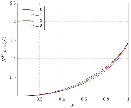
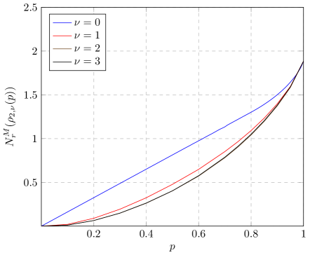
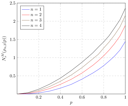
Another example of Fock diagonal state is a noisy Fock state, e.g., a Fock state mixed with a certain amount of thermal noise. These states, herafter called noisy Fock states, are defined by
| (82) |
where the thermal state is given in (37). In principle, we can approximate the exact value of with arbitrary precision for any and , as pointed out in Remark 45. Let us first consider the simpler case , which is a good approximation in certain regimes, e.g., optical frequencies at room temperature. The state then becomes , and thanks to Proposition 44 we can assume to be in the form (we already exploited the scale invariance). Now we have to perform just two nested optimizations over one real parameter each, that is,
| (83) |
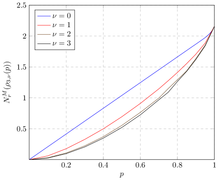
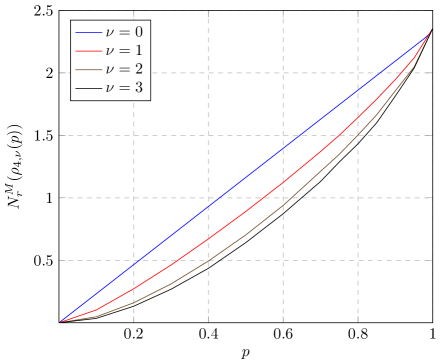
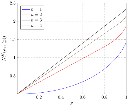
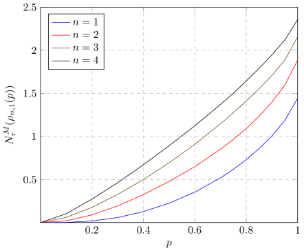
For the above program can even be solved analytically, since the inner maximization reduces to solving a -th order algebraic equation. For example, for one simply finds , and . The case of a nonzero temperature can be tackled by considering truncations of and performing numerical optimizations until some tolerance threshold is achieved. The results for different values of and are reported in Figures 2 and 3.

IX.2 Schrödinger cat states
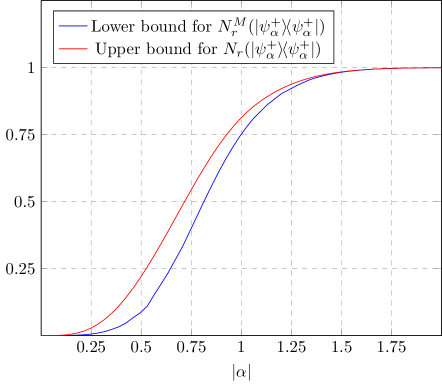
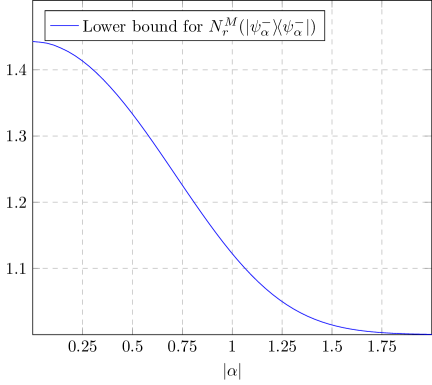
For , the associated Schrödinger cat states (or simply cat state) is defined by Dodonov et al. (1974)
| (84) |
It is a nonclassical state for all . Since a phase space rotation acts as , and all of our nonclassicality monotones are left invariant by such transformations, in what follows we can without loss of generality assume that . Now, for a cat state with real , we can consider the group and its representation given by the reflection with respect to the real and/or imaginary axis. Applying Corollary 43 to this setting (with ) shows immediately that (70)–(71) hold with and being the sets of classical states and bounded operators that are invariant under reflections with respect to the real and/or imaginary axis. A lower bound for can be easily computed by setting a maximum rank for in the second line of (71) and then optimizing numerically. When , in order to preserve the symmetry, must be supported on the subspace . Analogously, an upper bound for can be found with a classical belonging to . In Figure 4 we report these two bounds for the even cat state , and an analogous lower bound for .
IX.3 Squeezed states
A single-mode squeezed vacuum state is defined by (Barnett and Radmore, 2002, Eq. (3.7.5))
| (85) |
Since changing amounts to a simple rotation in phase space, and this cannot modify the value of any of our nonclassicality monotones, we will assume from now on. A squeezed state has always finite energy , and hence we can use Proposition 30 to get the upper bound
A second upper bound on can be found by considering a (classical) squeezed thermal state
where is the usual squeezing unitary with real parameter , and plugging it in the infimum that defines (cf. (21)), i.e.,
where . The rightmost side of the above expression can be easily optimized numerically. A lower bound on can be found from Corollary 41. All these estimates are plotted in Figure 5.
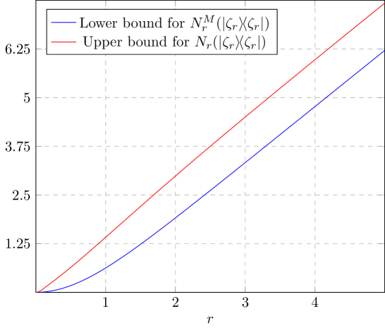
IX.4 Fock state dilution
Now we are ready to report an example in which the bound in Theorem 23 is (asymptotically) tight.
Proposition 47.
Proof.
We start with the lower bound. Consider the following protocol, implemented with only linear optics, destructive measurements, and feed forward.
-
(1)
We send into a beam splitter with transmissivity whose second mode’s initial state is the vacuum.
-
(2)
We perform photon counting on the ancillary mode.
-
(3)
If we measure 0 photons, the output state of the remaining mode is , with . We restart with step (1).
-
(4)
If we measure 1 photon, the output state of the remaining mode is , and we have succeeded.
-
(5)
If we measure 2 or more photons, the protocol is aborted.
Using the well-known formula Kim et al. (2002)
| (87) |
a lengthy but straightforward calculation shows that the global probability of success of this protocol is
| (88) |
Since we can take arbitrarily close to , we see that
which proves the lower bound.
IX.5 Cat state manipulation
Let us now discuss some protocols to transform cat states, enlarging or reducing their amplitude . Hereafter we take without loss of generality to be real. The first transformation we consider is amplification: . Lund et al. Lund et al. (2004) have provided a protocol that achieves exact conversion of two copies of the initial state with probability
| (89) |
Hence,
| (90) |
Mimicking the protocol of Lund et al. but employing slightly better (yet less realistic) measurements, we are able to obtain a better bound.
Proposition 48.
In the QRT of nonclassicality it is possible to achieve exact conversion with probability
| (91) |
Therefore,
| (92) |
Proof.
Consider the following protocol. Apply a beam splitter with trasmissivity to the initial state . Using (76), we obtain that
Carrying out on the second mode the measurement , with
yields
where the subscripts identify different modes. Computing the norm of the above vector yields (91) and this in turn (92). ∎
We now move on to cat state dilution. We consider the slightly simpler task of balanced dilution .
Proposition 49.
In the QRT of nonclassicality it holds that
| (93) |
Proof.
Consider the following protocol. Apply a beam splitter with trasmissivity to the initial state . Using one again (76), we obtain that
Therefore, measuring the second mode in the orthonormal basis whose first two elements are and , we obtain that
Computing the norms of the vectors on the right-hand side yields the estimates
Applying the above protocol to copies of yields, in the limit of large , at least copies of . Hence,
which completes the proof. ∎
X Acknowledgments
GF and LL dedicate this work to the memory of Piero Angela, whose career devoted to the popularization of science, spanning more than 50 years, was of immense inspiration for generations of Italian scientists Nosengo (2022). GF and LL contributed equally to this paper. LL is grateful to Krishna Kumar Sabapathy and Andreas Winter for enlightening discussions on the computation of the relative entropy of nonclassicality for Fock states. LL and MBP are supported by the ERC Synergy Grant BioQ (grant no. 319130) and HyperQ (grant no. 856432). LL thanks also the Alexander von Humboldt Foundation. GF acknowledges the support received from the EU through the ERASMUS+ Traineeship program and from the Scuola Galileiana di Studi Superiori.
Competing interest — The authors declare no competing interests.
Data availability — No data sets were generated during this study.
Appendix A Restricted asymptotic continuity in infinite dimensions
Among the many properties that a monotone may have, one of the most desirable is, in many scenarios, some form of continuity, since it allows to relate the resource content of a state to that of a “good” approximation of it. The most widely used notion of continuity, when it comes to resource monotones in finite-dimensional QRT, is that of asymptotic continuity Synak-Radtke and Horodecki (2006) (Definition 6(c)). Its popularity is due to its role in proving bounds on asymptotic rates. Of course, the notion of asymptotic continuity becomes empty in infinite dimensions, ultimately leading to the “asymptotic continuity catastrophe” discussed in the Introduction. In this Appendix, we show how asymptotic continuity can be defined in a certain sense for infinite-dimensional systems as well, why this extension presents some substantial limitations, and in which sense Theorem 15 overcomes such limitations.
A.1 Abstract approach
The traditional approach to the problem of bounding asymptotic transformation rates in infinite-dimensional QRTs makes use of the notion of restricted asymptotic continuity Eisert et al. (2002); Shirokov (2016a, 2018, 2020a, 2020b). Let us give a formal definition, taken from (Shirokov, 2016a, Corollary 7).
Definition A50.
Let be a QRT equipped with a monotone . For some , fix a family of states , with . We say that is weakly asymptotically continuous on if for all sequence of states and with and it holds that
| (A94) |
Formally, from the above definition the following can be deduced.
Proposition A51.
Let be a QRT equipped with a weakly additive monotone . Consider , and assume that there exists a family of states on which is weakly asymptotically continuous. Pick and with for all sufficiently large , and consider the modified asymptotic transformation rate
| (A95) |
Then it satisfies:
| (A96) |
whenever the right-hand side is well defined.555This just means that it does not contain the fractions or . We instead convene that and .
Proof.
For any sequence of free operations satisfying
it holds that
Here, 1 follows from weak additivity, 2 from monotonicity, and 3 from weak asymptotic continuity and again weak additivity. ∎
A.2 A physically interesting case: energy-constrained asymptotic continuity
The above definition may seem rather abstract. However, there is a physically very natural scenario where it can be applied. Let us assume that a certain system is equipped with a Hamiltonian (i.e., a self-adjoint operator) . Let us assume that the Hamiltonians add up without interaction terms upon taking multiple copies of , in formula . Now, for a real number , set
| (A97) |
Basically, we are considering states whose energy increases at most linearly in the number of systems . When the set (A97) is chosen in Definition A50, the corresponding notion of weakly asymptotic continuity becomes a physically relevant and indeed fruitful one.
Definition A52.
Let be a QRT endowed with a monotone . Let be equipped with a Hamiltonian . If for all the monotone is weakly asymptotically continuous on the set defined by (A97), then we say that it is asymptotically continuous in the presence of an energy constraint, or EC asymptotically continuous for short.
In practice, the above definition just means that whenever and are sequences of states with , (for a fixed but arbitrary real number ), and moreover , then
| (A98) |
This definition turns out to encompass a sufficiently wide set of monotones. For example, Shirokov has proved that many important entanglement monotones are EC asymptotically continuous, with respect to several physically relevant Hamiltonians Shirokov (2016a, 2018, 2020a, 2020b). To deduce a useful result from Proposition A51 we need to fix some terminology.
Definition A53 ((Winter, 2017, p. 9)).
Let be two quantum system equipped with Hamiltonians . A quantum channel from to is called -energy-limited if , with being the adjoint of . The set of such channels will be denoted with , where the choice of the Hamiltonians is not made explicit and assumed to be clear from the context.
In such a setting, directly from Proposition A51 we deduce the following.
Proposition A54.
Let be a QRT. Let be two Hamiltonians on , and let be a weakly additive monotone that is EC asymptotically continuous. Then for all and with finite energy (i.e., such that ) the uniformly energy-constrained (UEC) asymptotic transformation rate defined by
| (A99) |
satisfies that
| (A100) |
whenever the right-hand side is well defined.
Proof.
The reason why Proposition A54 is ultimately not satisfactory, and why we on the contrary deem Theorem 15 more compelling, is twofold. First, Proposition A54 only allows us to bound the standard asymptotic transformation rate (Definition 10), while we have seen that in certain settings the relevant quantity is the maximal asymptotic transformation rate (Definition 11). Secondly, the above result only takes into account sequences of protocols that are uniformly energy-constrained, meaning that the output energy is at most , with and fixed for the whole sequence. If each is -energy-limited for each , but or , the above method does not seem to tell us much about the corresponding rate, even when the initial and final states have a fixed (and finite) energy. Therefore, for instance, a sequence of free operations on CV systems where each involves either (a) a squeezing whose intensity increases with and tends to in the limit ; or (b) a displacement unitary whose parameter is superlinear in , are excluded from the bound in Proposition A54.
As we have seen, our Theorem 15 eliminates the need for both of these requirements, and instead provides ultimate bounds on maximal (instead of standard) asymptotic transformation rates, in a setting where the free protocols employed are otherwise totally unconstrained.
Appendix B Approximation by spectral truncation
Here we study the problem of approximating by truncating the input state. The forthcoming Corollary A58 has been used to check the numerical validity of the plots in Section IX.1 We state first a useful lemma, whose proof follows closely that of (Winter, 2016, Lemma 7), with some adaptations made to fit our infinite-dimensional case. In what follows, for a trace class operator with decomposition into positive and negative parts, we denote with its absolute value.
Lemma A55.
Let be two -mode states, and set . Assume that the operator has finite mean photon number . Then, for it holds that
| (A101) |
where .
Remark A56.
Recently, Shirokov Shirokov (2018) has put forward a more general technique that allows to obtain general continuity results for relative entropy distance measures in infinite dimensions, thus removing the need to make any assumption concerning the operator . While theoretically superior, his bounds are less tight and ultimately not suited for our practical purposes.
Proof of Lemma A55.
We start with the case where . Here we actually prove that
| (A102) |
for all -mode auxiliary states . Call the binary entropy function. Using the convexity of (Lemma 28) together with (Ohya and Petz, 2004, Proposition 5.24), it is not difficult to observe, as done by Winter (Winter, 2016, Lemma 7), that
| (A103) |
We now construct two states such that
In particular, the mean photon number of satisfies that
Now, set
Then, on the one hand
Here, the estimate in 1 comes from convexity (A103), while that in 2 is an application of the subadditivity of (Lemma 28) together with Proposition 30. On the other hand, we can write
where the inequality in 3 is the lower bound in (A103), and that in 4 holds because of the monotonicity of under the classical operation of tracing away subsystems. Putting all together we see that
Together with the corresponding inequality with and exchanged, this yields (A102), and in particular proves (A101) for .
Remark A57.
The application of Lemma A55 that is of interest to us is as follows.
Corollary A58.
Let be two -mode states, and set . Assume that and also . Then, for it holds that
| (A104) |
where again . In particular, denoting with the spectral decomposition of , the sequence of spectral truncations satisfies that
| (A105) |
Appendix C A technical lemma
The following result was invoked in the proof of Proposition 40 (more precisely, in step 3 of (66)) as an alternative to (Ohya and Petz, 2004, Proposition 5.23(iv)). For the sake of completeness, we include a proof.
Lemma A59.
Let us consider two -mode states , with . Then, it holds that
Proof.
At fist sight, the result might seem a trivial application of the definitions of measured relative entropy as given in (10) and of heterodyne detection as given in (Serafini, 2017, 5.4.2). The only obstacle is that, according to our definition, a POVM must be a finite collection of operators; this is also crucial for proving Lemma 20, and hence cannot be simply removed. The idea of the proof is precisely to show that an heterodyne detection, which corresponds to the decomposition of the identity , can be approximated, inside the Kullback–Leibler divergence, by a sequence of finite POVMs. Note that the hypothesis is needed to ensure that is a well-defined Lebesgue integral for any (possibly diverging to ).
Let us fix and consider the family of subsets of , , with a finite positive integer, constructed as follows:
-
•
-
•
For , is a subset of such that:
-
–
it is contained in a ball of radius ;
-
–
if ;
-
–
and , where is the -dimensional ball with radius and centered at the origin of .
-
–
-
•
.
Notice that we do not specify the dependence of upon and for ease of notation. It is clear from the definition that the set , with
is a proper, finite POVM.
For a fixed state we can compute the classical probability distribution
Since , we can always take big enough so that . Similarly we can always choose such that . Now, given another fixed state , we have:
Here, in 1 we have discarded two positive terms, in 2 we have used the fact that and , in 3 we have used the fact that and are uniformly continuous on any compact set and finally in 4 we have used the fact that also the logarithm is uniformly continuous on . Now, by taking the proper limits, i.e., and , we obtain precisely the generalized Riemann integral over of the function . Since , the function is absolutely integrable, and the generalized Riemann integral is well defined and coincides with the Lebesgue one. ∎
References
- Bennett (2004) C. H. Bennett, Quantum Inf. Comput. 4, 460 (2004).
- Coecke et al. (2016) B. Coecke, T. Fritz, and R. W. Spekkens, Inf. Comput. 250, 59 (2016).
- Chitambar and Gour (2019) E. Chitambar and G. Gour, Rev. Mod. Phys. 91, 025001 (2019).
- Shannon (1948) C. E. Shannon, Bell Syst. Tech. J. 27, 379 (1948).
- Cover and Thomas (2006) T. M. Cover and J. A. Thomas, Elements of Information Theory, Wiley Series in Telecommunications and Signal Processing (Wiley-Interscience, New York, NY, USA, 2006).
- Bennett et al. (1996a) C. H. Bennett, H. J. Bernstein, S. Popescu, and B. Schumacher, Phys. Rev. A 53, 2046 (1996a).
- Plenio and Virmani (2007) M. B. Plenio and S. Virmani, Quantum Inf. Comput. 7, 1 (2007).
- Horodecki et al. (2009) R. Horodecki, P. Horodecki, M. Horodecki, and K. Horodecki, Rev. Mod. Phys. 81, 865 (2009).
- Vidal (2000) G. Vidal, J. Mod. Opt. 47, 355 (2000).
- Horodecki et al. (2000) M. Horodecki, P. Horodecki, and R. Horodecki, Phys. Rev. Lett. 84, 2014 (2000).
- Donald et al. (2002) M. J. Donald, M. Horodecki, and O. Rudolph, J. Math. Phys. 43, 4252 (2002).
- Horodecki (2001) M. Horodecki, Quantum Inf. Comput. 1, 3 (2001).
- Synak-Radtke and Horodecki (2006) B. Synak-Radtke and M. Horodecki, J. Phys. A 39, L423 (2006).
- Wehrl (1976) A. Wehrl, Rep. Math. Phys. 10, 159 (1976).
- Wehrl (1978) A. Wehrl, Rev. Mod. Phys. 50, 221 (1978).
- Eisert et al. (2002) J. Eisert, C. Simon, and M. B. Plenio, J. Phys. A 35, 3911 (2002).
- Shirokov (2018) M. E. Shirokov, Rep. Math. Phys. 81, 81 (2018).
- Shirokov (2020a) M. E. Shirokov, Quantum Inf. Process. 19, 164 (2020a).
- Shirokov (2020b) M. E. Shirokov, Preprint arXiv:2007.00417 (2020b).
- Braunstein and van Loock (2005) S. L. Braunstein and P. van Loock, Rev. Mod. Phys. 77, 513 (2005).
- Cerf et al. (2007) N. J. Cerf, G. Leuchs, and E. S. Polzik, Quantum information with continuous variables of atoms and light (Imperial College Press, 2007).
- Weedbrook et al. (2012) C. Weedbrook, S. Pirandola, R. García-Patrón, N. J. Cerf, T. C. Ralph, J. H. Shapiro, and S. Lloyd, Rev. Mod. Phys. 84, 621 (2012).
- Sperling and Vogel (2015) J. Sperling and W. Vogel, Phys. Scr. 90, 074024 (2015).
- Tan et al. (2017) K. C. Tan, T. Volkoff, H. Kwon, and H. Jeong, Phys. Rev. Lett. 119, 190405 (2017).
- Yadin et al. (2018) B. Yadin, F. C. Binder, J. Thompson, V. Narasimhachar, M. Gu, and M. S. Kim, Phys. Rev. X 8, 041038 (2018).
- Tan and Jeong (2019) K. C. Tan and H. Jeong, AVS Quantum Sci. 1, 014701 (2019).
- Lami et al. (2021) L. Lami, B. Regula, R. Takagi, and G. Ferrari, Phys. Rev. A 103, 032424 (2021).
- Regula et al. (2021) B. Regula, L. Lami, R. Takagi, and G. Ferrari, Phys. Rev. Lett. 126, 110403 (2021).
- Brandão et al. (2013) F. G. S. L. Brandão, M. Horodecki, J. Oppenheim, J. M. Renes, and R. W. Spekkens, Phys. Rev. Lett. 111, 250404 (2013).
- Goold et al. (2016) J. Goold, M. Huber, A. Riera, L. del Rio, and P. Skrzypczyk, J. Phys. A 49, 143001 (2016).
- Tucci (1999) R. R. Tucci, Preprint arXiv:quant-ph/9909041 (1999).
- Christandl and Winter (2004) M. Christandl and A. Winter, J. Math. Phys. 45, 829 (2004).
- Brandão et al. (2011) F. G. S. L. Brandão, M. Christandl, and J. Yard, Commun. Math. Phys. 306, 805 (2011).
- Li and Winter (2014) K. Li and A. Winter, Commun. Math. Phys. 326, 63 (2014).
- Shirokov (2016a) M. E. Shirokov, J. Math. Phys. 57, 032203 (2016a).
- Wikipedia contributors (2017) Wikipedia contributors, “Operator topologies — Wikipedia, the free encyclopedia,” https://en.wikipedia.org/w/index.php?title=Operator_topologies&oldid=792420018 (2017), [Online; accessed 29-October-2019].
- Davies (1969) E. B. Davies, Commun. Math. Phys. 15, 277 (1969).
- Winter (1999) A. Winter, IEEE Trans. Inf. Theory 45, 2481 (1999).
- Schrödinger (1926) E. Schrödinger, Naturwissenschaften 14, 664 (1926).
- Klauder (1960) J. R. Klauder, Ann. Phys. (N. Y.) 11, 123 (1960).
- Glauber (1963) R. J. Glauber, Phys. Rev. 131, 2766 (1963).
- Sudarshan (1963) E. C. G. Sudarshan, Phys. Rev. Lett. 10, 277 (1963).
- Husimi (1940) K. Husimi, Proc. Phys.-Math. Soc. Jpn. 22, 264 (1940).
- Umegaki (1962) H. Umegaki, Kodai Math. Sem. Rep. 14, 59 (1962).
- Ohya and Petz (2004) M. Ohya and D. Petz, Quantum Entropy and Its Use, Theoretical and Mathematical Physics (Springer Berlin Heidelberg, 2004).
- Lindblad (1973) G. Lindblad, Commun. Math. Phys. 33, 305 (1973).
- Hiai and Petz (1991) F. Hiai and D. Petz, Comm. Math. Phys. 143, 99 (1991).
- Buscemi et al. (2019) F. Buscemi, D. Sutter, and M. Tomamichel, Quantum 3, 209 (2019).
- Wang and Wilde (2019) X. Wang and M. M. Wilde, Phys. Rev. Research 1, 033169 (2019).
- Kullback and Leibler (1951) S. Kullback and R. A. Leibler, Ann. Math. Statist. 22, 79 (1951).
- Donald (1986) M. J. Donald, Commun. Math. Phys. 105, 13 (1986).
- Petz (1986) D. Petz, Commun. Math. Phys. 105, 123 (1986).
- Berta et al. (2017) M. Berta, O. Fawzi, and M. Tomamichel, Lett. Math. Phys. 107, 2239 (2017).
- Bennett et al. (1996b) C. H. Bennett, G. Brassard, S. Popescu, B. Schumacher, J. A. Smolin, and W. K. Wootters, Phys. Rev. Lett. 76, 722 (1996b).
- Eisert and Plenio (2003) J. Eisert and M. B. Plenio, Int. J. Quantum Inf. 1, 479 (2003).
- Shirokov (2016b) M. E. Shirokov, Mat. Sb. 207, 724 (2016b).
- Werner and Wolf (2001) R. F. Werner and M. M. Wolf, Phys. Rev. Lett. 86, 3658 (2001).
- Giedke et al. (2001) G. Giedke, B. Kraus, M. Lewenstein, and J. I. Cirac, Phys. Rev. Lett. 87, 167904 (2001).
- Giedke et al. (2003) G. Giedke, J. Eisert, I. J. Cirac, and M. B. Plenio, Quantum Inf. Comput. 3, 211 (2003).
- Adesso and Illuminati (2007) G. Adesso and F. Illuminati, J. Phys. A 40, 7821 (2007).
- Lami et al. (2018) L. Lami, A. Serafini, and G. Adesso, New J. Phys. 20, 023030 (2018).
- Narasimhachar et al. (2021) V. Narasimhachar, S. Assad, F. C. Binder, J. Thompson, B. Yadin, and M. Gu, npj Quantum Inf. 7, 9 (2021).
- Serafini et al. (2020) A. Serafini, M. Lostaglio, S. Longden, U. Shackerley-Bennett, C.-Y. Hsieh, and G. Adesso, Phys. Rev. Lett. 124, 010602 (2020).
- Knill et al. (2001) E. Knill, R. Laflamme, and G. J. Milburn, Nature 409, 46 (2001).
- Eisaman et al. (2011) M. D. Eisaman, J. Fan, A. Migdall, and S. V. Polyakov, Rev. Sci. Instrum. 82, 071101 (2011).
- Kennard (1927) E. H. Kennard, Z. Phys. 44, 326 (1927).
- Walls (1983) D. F. Walls, Nature 306, 141 (1983).
- Slusher et al. (1985) R. E. Slusher, L. W. Hollberg, B. Yurke, J. C. Mertz, and J. F. Valley, Phys. Rev. Lett. 55, 2409 (1985).
- Andersen et al. (2016) U. L. Andersen, T. Gehring, C. Marquardt, and G. Leuchs, Phys. Scr. 91, 053001 (2016).
- Schnabel (2017) R. Schnabel, Phys. Rep. 684, 1 (2017).
- Dodonov et al. (1974) V. V. Dodonov, I. A. Malkin, and V. I. Man’ko, Physica 72, 597 (1974).
- Ralph et al. (2003) T. C. Ralph, A. Gilchrist, G. J. Milburn, W. J. Munro, and S. Glancy, Phys. Rev. A 68, 042319 (2003).
- Lund et al. (2008) A. P. Lund, T. C. Ralph, and H. L. Haselgrove, Phys. Rev. Lett. 100, 030503 (2008).
- Joo et al. (2011) J. Joo, W. J. Munro, and T. P. Spiller, Phys. Rev. Lett. 107, 083601 (2011).
- Facon et al. (2016) A. Facon, E.-K. Dietsche, D. Grosso, S. Haroche, J.-M. Raimond, M. Brune, and S. Gleyzes, Nature 535, 262 (2016).
- Brask et al. (2010) J. B. Brask, I. Rigas, E. S. Polzik, U. L. Andersen, and A. S. Sørensen, Phys. Rev. Lett. 105, 160501 (2010).
- Lee and Jeong (2013) S.-W. Lee and H. Jeong, Phys. Rev. A 87, 022326 (2013).
- Sychev et al. (2017) D. V. Sychev, A. E. Ulanov, A. A. Pushkina, M. W. Richards, I. A. Fedorov, and A. I. Lvovsky, Nat. Photonics 11, 379 (2017).
- Sanders (1989) B. C. Sanders, Phys. Rev. A 40, 2417 (1989).
- Dowling (2008) J. P. Dowling, Contemp. Phys. 49, 125 (2008).
- Vidal and Werner (2002) G. Vidal and R. F. Werner, Phys. Rev. A 65, 032314 (2002).
- Plenio (2005) M. B. Plenio, Phys. Rev. Lett. 95, 090503 (2005).
- Lami and Regula (2021) L. Lami and B. Regula, Preprint arXiv:2111.02438 (2021), 10.48550/arXiv.2111.02438.
- Hillery (1987) M. Hillery, Phys. Rev. A 35, 725 (1987).
- Dodonov et al. (2000) V. V. Dodonov, O. V. Man’ko, M. V. I., and A. Wünsche, J. Mod. Opt. 47, 633 (2000).
- Marian et al. (2004) P. Marian, T. A. Marian, and H. Scutaru, Phys. Rev. A 69, 022104 (2004).
- Brandão and Plenio (2008) F. G. S. L. Brandão and M. B. Plenio, Nat. Phys. 4, 873 (2008).
- Lee (1991) C. Lee, Phys. Rev. A 44, R2775 (1991).
- Lütkenhaus and Barnett (1995) N. Lütkenhaus and S. M. Barnett, Phys. Rev. A 51, 3340 (1995).
- Asbóth et al. (2005) J. K. Asbóth, J. Calsamiglia, and H. Ritsch, Phys. Rev. Lett. 94, 173602 (2005).
- Vogel and Sperling (2014) W. Vogel and J. Sperling, Phys. Rev. A 89, 052302 (2014).
- Killoran et al. (2016) N. Killoran, F. E. S. Steinhoff, and M. B. Plenio, Phys. Rev. Lett. 116, 080402 (2016).
- Kwon et al. (2019) H. Kwon, K. C. Tan, T. Volkoff, and H. Jeong, Phys. Rev. Lett. 122, 040503 (2019).
- Kenfack and Życzkowski (2004) A. Kenfack and K. Życzkowski, J. Opt. B 6, 396 (2004).
- Tan et al. (2020) K. C. Tan, S. Choi, and H. Jeong, Phys. Rev. Lett. 124, 110404 (2020).
- Vogel (2000a) W. Vogel, Phys. Rev. Lett. 84, 1849 (2000a).
- Diósi (2000) L. Diósi, Phys. Rev. Lett. 85, 2841 (2000).
- Vogel (2000b) W. Vogel, Phys. Rev. Lett. 85, 2842 (2000b).
- Richter and Vogel (2002) T. Richter and W. Vogel, Phys. Rev. Lett. 89, 283601 (2002).
- Idel et al. (2016) M. Idel, D. Lercher, and M. M. Wolf, J. Phys. A 49, 445304 (2016).
- Bohmann and Agudelo (2020) M. Bohmann and E. Agudelo, Phys. Rev. Lett. 124, 133601 (2020).
- Gehrke et al. (2012) C. Gehrke, J. Sperling, and W. Vogel, Phys. Rev. A 86, 052118 (2012).
- Vedral et al. (1997) V. Vedral, M. B. Plenio, M. A. Rippin, and P. L. Knight, Phys. Rev. Lett. 78, 2275 (1997).
- Vedral and Plenio (1998) V. Vedral and M. B. Plenio, Phys. Rev. A 57, 1619 (1998).
- Fekete (1923) M. Fekete, Math. Z. 17, 228 (1923).
- Sion (1958) M. Sion, Pacific J. Math. 8, 171 (1958).
- Lund et al. (2004) A. P. Lund, H. Jeong, T. C. Ralph, and M. S. Kim, Phys. Rev. A 70, 020101 (2004).
- Laghaout et al. (2013) A. Laghaout, J. S. Neergaard-Nielsen, I. Rigas, C. Kragh, A. Tipsmark, and U. L. Andersen, Phys. Rev. A 87, 043826 (2013).
- Sychev et al. (2018) D. V. Sychev, A. E. Ulanov, A. A. Pushkina, I. A. Fedorov, M. W. Richards, P. Grangier, and A. I. Lvovsky, AIP Conf. Proc. 1936, 020018 (2018).
- Wang et al. (2018) M. Wang, Z. Qin, M. Zhang, L. Zeng, X. Su, C. Xie, and K. Peng, in 2018 Conference on Lasers and Electro-Optics (CLEO) (2018) pp. 1–2.
- Oh and Jeong (2018) C. Oh and H. Jeong, J. Opt. Soc. Am. B 35, 2933 (2018).
- Pinsker (1964) M. S. Pinsker, Information and Information Stability of Random Variables and Processes, edited by A. Feinstein, Holden-Day series in time series analysis (Holden-Day, 1964).
- Ruskai (1994) M. B. Ruskai, Rev. Math. Phys. 06, 1147 (1994).
- Lami (2020) L. Lami, IEEE Trans. Inf. Theory 66, 2165 (2020).
- Hall (2013) B. C. Hall, Quantum Theory for Mathematicians, Graduate Texts in Mathematics (Springer New York, 2013).
- Levi (1906) B. Levi, Rendic. Istit. Lombardo XXXIX, 775 (1906).
- Rudin (1964) W. Rudin, Principles of mathematical analysis, International series in pure and applied mathematics (McGraw-Hill, 1964).
- Hansen and Pedersen (2003) F. Hansen and G. K. Pedersen, Bull. Lond. Math. Soc. 35, 553 (2003).
- Seshadreesan and Wilde (2015) K. P. Seshadreesan and M. M. Wilde, Phys. Rev. A 92, 042321 (2015).
- Bach and Lüxmann-Ellinghaus (1986) A. Bach and U. Lüxmann-Ellinghaus, Commun. Math. Phys. 107, 553 (1986).
- Megginson (2012) R. E. Megginson, An introduction to Banach space theory, Graduate Texts in Mathematics No. 183 (Springer Science & Business Media, 2012).
- Lieb and Ruskai (1973a) E. H. Lieb and M. B. Ruskai, Phys. Rev. Lett. 30, 434 (1973a).
- Lieb and Ruskai (1973b) E. H. Lieb and M. B. Ruskai, J. Math. Phys. 14, 1938 (1973b).
- Lieb (1973) E. H. Lieb, Adv. Math. 11, 267 (1973).
- Lindblad (1975) G. Lindblad, Commun. Math. Phys. 40, 147 (1975).
- Serafini (2017) A. Serafini, Quantum Continuous Variables: A Primer of Theoretical Methods (CRC Press, Taylor & Francis Group, 2017).
- Barnett and Radmore (2002) S. Barnett and P. M. Radmore, Methods in Theoretical Quantum Optics, Oxford Series in Optical and Imaging Sciences (Clarendon Press, 2002).
- Kim et al. (2002) M. S. Kim, W. Son, V. Bužek, and P. L. Knight, Phys. Rev. A 65, 032323 (2002).
- Nosengo (2022) N. Nosengo, Nat. Italy (2022), 10.1038/d43978-022-00102-4.
- Winter (2017) A. Winter, Preprint arXiv:1712.10267 (2017), 10.48550/arXiv.1712.10267.
- Winter (2016) A. Winter, Commun. Math. Phys. 347, 291 (2016).