Three-dimensional shear driven turbulence with noise at the boundary

Abstract.

We consider the incompressible 3D Navier-Stokes equations subject to a shear induced by noisy movement of part of the boundary. The effect of the noise is quantified by upper bounds on the first two moments of the dissipation rate. The expected value estimate is consistent with the Kolmogorov dissipation law, recovering an upper bound as in [DC92] for the deterministic case. The movement of the boundary is given by an Ornstein–Uhlenbeck process; a potential for over-dissipation is noted if the Ornstein–Uhlenbeck process were replaced by the Wiener process.

1. INTRODUCTION

Noise is added to turbulence models for a variety of reasons, both practical and theoretical. For example, the onset of turbulence is often related to the randomness of background movement [MR04]. In any turbulent flow there are unavoidably perturbations in boundary conditions and material properties; see [P00, Chapter 3]. The addition of noise in a physical model can be interpreted as a perturbation from the model. There is considerable evidence supporting the stabilization of solutions by noise (see, e.g., [B01, CLM01, FSQD19, K99]). However, the effect of noise in turbulent flow is far from completely understood.

This paper concerns the Kolmogorov dissipation law associated with the incompressible Navier-Stokes equations (NSE) in a 3-dimensional box $D=(0,L)^{2}\times(0,h)$ subject to a shear induced by noisy movement of one wall. Specifically, we consider the following differential equation,

(1.1) $$\begin{split}du+(u\cdot\nabla u-&\nu\Delta u+\nabla p)\,dt=0,\\ &\nabla\cdot u=0,\end{split}$$

with $L$-periodic boundary condition in the $x_{1}$ and $x_{2}$ directions and a random boundary condition given by the following: for all time $t\in\mathbb{R}_{+}$ and $(x_{1},x_{2})\in(0,L)^{2}$,

(1.2) $$\begin{split}u(x_{1},x_{2},0,t)=(\mathbb{X}_{t},0,0)^{\mathstrut\scriptscriptstyle\top}\hskip 18.0pt&\mbox{and}\hskip 18.0ptu(x_{1},x_{2},h,t)=(0,0,0)^{\mathstrut\scriptscriptstyle\top}\;.\end{split}$$

In the above, $\nu>0$ is a fixed real parameter representing the viscosity, and $\mathbb{X}=(\mathbb{X}_{t})_{t\in\mathbb{R}_{+}}$ is a given continuous-time, real-valued stochastic process. The stochastic processes $u$ and $p$ represent respectively the velocity field and the pressure.

The Kolmogorov dissipation law is tied to a phenomenon in turbulence called the energy cascade, which can be explained in 3 main steps. $1-$ In the absence of a body force, the kinetic energy is introduced into the large scales of the fluid between the parallel plates by the effects of the moving plate. This energy is called energy input. $2-$ The large eddies break up into smaller eddies through vortex stretching over an intermediate range, where the energy is transferred to smaller scales and the energy dissipation due to the viscous force is negligible. $3-$ At small enough scales (expected to be $\sim\text{Re}^{-3/4}$, where Re is the Reynolds number defined in (1.3)) dissipation dominates and the energy in those smallest scales decays to zero exponentially fast.

Based on the above description the dissipation is effective at the end of a sequence of processes. Therefore, the rate of dissipation, which measures the amount of energy lost by the viscous force, is determined by the first process in the sequence, which is the energy input. The persistent force driving the shear flow is the motion of the bottom wall $\{(x_{1},x_{2},0):\,(x_{1},x_{2})\in[0,L]^{2}\}$. The time averaged energy dissipation rate must balance the drag exerted by the walls on the fluid. In terms of the characteristic speed $U$, the large eddies have energy of order $U^{2}$ and time scale $\tau=h/U$, so the rate of energy input can be scaled as $U^{2}/\tau=U^{3}/h$. This suggests the Kolmogorov dissipation law for time-averaged energy dissipation rate $\varepsilon$ (Kolmogorov 1941);

$$\varepsilon\sim\frac{U^{3}}{h}.$$

Here $a\sim b$ means $a\lesssim b$ and $b\lesssim a$; $a\lesssim b$ means $a\leq c\,b$ for a nondimensional universal constant $c$.

The energy dissipation rate has been widely studied in the literature in the deterministic case [B70, DLPRSZ18, DF02, DR00, H72, L02, L16, AP17, AP19, AP20]. Doering and Constantin proved in [DC92] a rigorous asymptotic bound directly from the Navier-Stokes equations. Their bound is of the form

(1.3) $$\varepsilon\lesssim\frac{U^{3}}{h}\;,\quad\text{as}\ \text{Re}\to\infty,\quad\text{where}\quad\text{Re}=\frac{Uh}{\nu},\;$$

similar estimations have been proven by Kerswell [K97], Marchiano [M94], and Wang [W97] in more generality.

In this paper we choose $\mathbb{X}_{t}$ to be an Ornstein–Uhlenbeck process (OU process) satisfying (2.1). We derive an upper bound on the expected value of the energy dissipation rate as well as its second moment in terms of characteristics of the randomly moving bottom wall. Our estimate recovers (1.3) in the limit as the variance $\sigma^{2}$ of the noise tends to 0. The key to the analysis is the choice of a stochastic background flow and the treatment of a stochastic integral (with respect to the Wiener process) as a local martingale.

Since the work of Bensoussan and Temam [BT73] in 1973, there has been substantial advance in understanding the stochastic Navier-Stokes equations, see for example [BCPW19, B00, BP00, MR04, MR05, WW15] and the references therein. Recently in [CP20], the exact dissipation rate is obtained for the stochastically forced Navier-Stokes equations under an assumption of energy balance. In all those works the equation always contains noise as a forcing term. Other than the analysis of symmetries of a passive scalar advected by a shear flow in which a boundary moves as a stochastic process in [CamassaKilicMcLaughlin19], to the best of our knowledge, there is no other work concerning the equations of the motion with stochastic boundary conditions.

Organization of this paper

In section 2, we will introduce the necessary notation and preliminary results needed in the proceeding sections. In section 3, we will state the main result of this work. We will set up an almost sure bound starting from the energy equation in section 4. From there, we will derive an upper bound on the mean value and variance of the energy dissipation respectively in sections 5 and 6. The concluding Section 7 contains some open problems in this direction.

2. Definitions and Notations

In this paper, we choose $\mathbb{X}_{t}$ to be an Ornstein–Uhlenbeck process (OU process), which is a diffusion process solving the Itô stochastic differential equation

(2.1) $$d\mathbb{X}_{t}=\theta(U-\mathbb{X}_{t})dt+\sigma dW_{t},$$

where $W=(W_{t})_{t\in\mathbb{R}_{+}}$ is a standard Brownian motion (a.k.a. the Wiener process), and $\theta>0$ and $\sigma>0$ are parameters. A strong solution to (2.1) is given by

$$\mathbb{X}_{t}=\mathbb{X}_{0}\,e^{-\theta t}+U\,(1-e^{-\theta t})+\sigma\int_{0}^{t}e^{-\theta(t-s)}\,dW_{s}.$$

It is well known that $\mathbb{X}_{t}$ has stationary distribution given by the normal distribution $\mathcal{N}(U,\frac{\sigma^{2}}{2\theta})$ with mean $U$ and variance $\frac{\sigma^{2}}{2\theta}$. If the initial distribution satisfies $\mathbb{X}_{0}\sim\mathcal{N}(U,\frac{\sigma^{2}}{2\theta})$, then $\mathbb{X}_{t}\sim N(U,\frac{\sigma^{2}}{2\theta})$ for all $t\geq 0$ and we say $\mathbb{X}$ is a stationary OU process.

Intuitively, the OU process is a Wiener process plus a tendency to move towards a location $U$, where the tendency is greater when the process is further away from that location. In (2.1), $\theta$ is the decay-rate which measures how strongly the system reacts to perturbations, and $\sigma^{2}$ is the variation or the size of the noise. We will need the following basic properties of the stationary OU process (for a proof and additional properties see [Doob42]).

Proposition 2.1.

Let $\mathbb{X}_{t}$ be a stationary Ornstein–Uhlenbeck process satisfying (2.1). The following hold for all $t\geq 0$.

1. $\mathbb{X}_{t}\sim N(U,\frac{\sigma^{2}}{2\theta})$ ,

2. $[\mathbb{X}]_{t}=\sigma^{2}\,t$, where $[\mathbb{X}]_{t}$ is the quadratic variation of $\mathbb{X}$ on $[0,t]$.

Throughout this manuscript, the $L^{2}(D)$ norm and inner product will be denoted by $\|\cdot\|$ and $(\cdot,\cdot)$ respectively. For the sake of boundary conditions, we consider

$$H=\{v\in[L^{2}(D)]^{3}:\,\nabla\cdot v=0,\,v(x_{1},x_{2},0)=v(x_{1},x_{2},h)=0,\,v\text{ periodic in }x_{1},x_{2}\},$$

$$V=\{v\in[H^{1}(D)]^{3}:\,\nabla\cdot v=0,\,v(x_{1},x_{2},0)=v(x_{1},x_{2},h)=0,\,v\text{ periodic in }x_{1},x_{2}\},$$

$$C^{\infty}_{\text{div}}=\{v\in[C^{\infty}(D)]^{3}:\,\nabla\cdot v=0,\,v(x_{1},x_{2},0)=v(x_{1},x_{2},h)=0,\,v\text{ periodic in }x_{1},x_{2}\}.$$

Stochastic Background Flow

The difficulty in the analysis of the shear flow (1.2) is due to the effect of the random inhomogeneous boundary condition. We overcome this difficulty by constructing a carefully chosen stochastic background flow. This construction is based on the Hopf extension [H55].

Our key idea here is to choose the boundary layer thickness $\delta_{t}$ in the background flow to be random and time-dependent, namely,

(2.2) $$\delta_{t}=\delta(\mathbb{X}_{t}(\omega))=\frac{A}{|\mathbb{X}_{t}(\omega)|^{2}+B}$$

where $\delta:\,\mathbb{R}\to(0,\infty)$ is the function $\delta(z)=\frac{A}{z^{2}+B}$. We later choose $A=\nu U$ and $B=U^{2}$, so $\delta_{t}$ has the dimension of length and $\delta_{t}\in(0,h)$ if $\text{Re}=\frac{U\,h}{\nu}>1$; see Lemma 4.3 for precise requirements.

We then let $\phi:\,[0,h]\times\mathbb{R}\to\mathbb{R}$ be the function

$$\phi(a,z)=\left(1-\dfrac{a}{\delta(z)}\right)z\,1_{\{0\leq a\leq\delta(z)\}}.$$

By definition, we have (see Figure 1)

(2.3) $$\phi(x_{3},\mathbb{X}_{t}(\omega))=\left\{\begin{array}[]{ll}\left(1-\dfrac{x_{3}}{\delta_{t}}\right)\mathbb{X}_{t}(\omega)&\mbox{if }0\leq x_{3}\leq\delta_{t}\\ 0&\mbox{if }\delta_{t}\leq x_{3}\leq h\end{array}.\right.$$

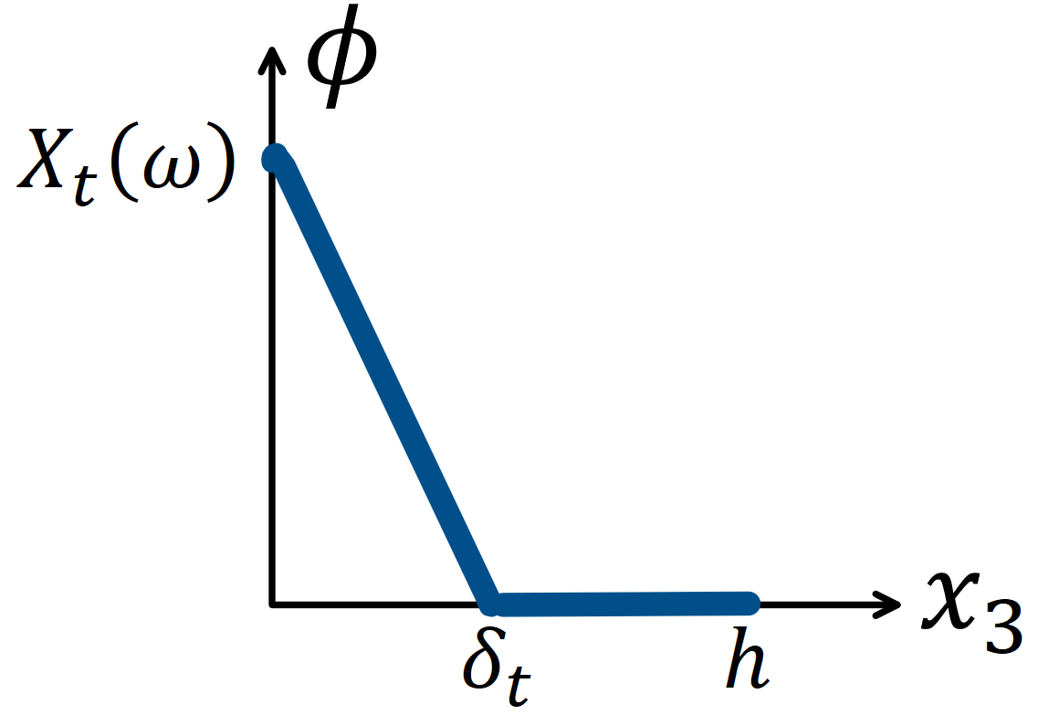
Figure 1. The graph of $x_{3}\mapsto\phi(x_{3},\mathbb{X}_{t}(\omega))$, where $\delta_{t}=\delta(\mathbb{X}_{t}(\omega))$ is the boundary layer thickness.

Finally, we define the stochastic background flow $\Phi=\Phi_{t}(x_{1},x_{2},x_{3};\omega)$ as

(2.4) $$\Phi_{t}(x_{1},x_{2},x_{3};\omega):=\big{(}\phi(x_{3},\mathbb{X}_{t}(\omega)),\;0,\;0\big{)}^{\mathstrut\scriptscriptstyle\top}.$$

There can be other choices for the function $\delta_{t}$, and our choice in (2.2) is motivated by the general analysis in (4.19). The boundary layer is denoted by $D_{\delta}=(0,L)^{2}\times(0,\delta_{t})$.

Martingale solutions

We follow the standard notion of martingale solutions for stochastic Naiver Stokes equations such as Flandoli and Gatarek [FG95, Definition 3.1], and define a martingale solution for our system (1.1)-(1.2). This notion is a probabilistically weak analogue of the Leray-Hopf weak solution to the deterministic Navier–Stokes equations.

Definition 2.1 (Martingale solution on compact intervals).

Let $T\in[0,\infty)$. A martingale solution to (1.1)-(1.2) on $[0,T]$ consists of a stochastic basis $\big{(}\Omega,\,(\mathcal{F}_{t})_{t\in[0,T]},\,\mathbb{P}\big{)}$ with a complete right-continuous filtration $(\mathcal{F}_{t})_{t\in[0,T]}$, a stationary OU process $(\mathbb{X}_{t})_{t\in[0,T]}$ adapted to $(\mathcal{F}_{t})_{t\in[0,T]}$, and with mean $U$ and variance $\frac{\sigma^{2}}{2\theta}$, and an $\mathcal{F}_{t}$-progressively measurable stochastic process

$$u:\;[0,T]\times\Omega\rightarrow[L^{2}(D)]^{3}$$

such that

• $u-\Phi$ has sample paths in $L^{2}\left([0,T];\,V\right)\cap L^{\infty}\left([0,T];\,H\right)$ almost surely,

• for all $t\in[0,T]$ and all $\varphi\in C^{\infty}_{\text{div}}$, the following identity holds almost surely,

  (2.5) $$(u(t),\varphi)+\nu\int_{0}^{t}(\nabla u(s),\nabla\varphi)\,ds+\int_{0}^{t}(u(s)\cdot\nabla u(s),\varphi)\,ds=(u(0),\varphi),$$

• the following holds

  (2.6) $$\mathbb{E}\left[\sup_{s\in[0,T]}\|u(s)\|^{2}+\int_{0}^{T}\|\nabla u(s)\|^{2}\,dt\right]\,<\infty.$$

Remark 2.2.

The existence of a martingale solution under the current assumptions can be derived by modifying a classical result of Flandoli and Gatarek [FG95] in the case when $\mathbb{X}_{t}=0$. As in the deterministic case, the uniqueness of such solutions is an open problem.

Remark 2.3.

Note that above solution is independent of the choice of $\Phi$ and depends only on the value of $\Phi$ on the boundary; see for instance [BH10, Chapter 9].

Essentially, a global solution has a fixed stochastic basis over $[0,\infty)$ which, when restricted to $[0,T]$, yields a solution as in Definition 2.1.

Definition 2.2 (Martingale solution).

A martingale solution to (1.1)-(1.2) consists of a stochastic basis $\big{(}\Omega,\,(\mathcal{F}_{t})_{t\in[0,\infty)},\,\mathbb{P}\big{)}$ with a complete right-continuous filtration $(\mathcal{F}_{t})_{t\in\mathbb{R}_{+}}$, a stationary OU process $\mathbb{X}=(\mathbb{X}_{t})_{t\in\mathbb{R}_{+}}$ with mean $U$ and variance $\frac{\sigma^{2}}{2\theta}$, and an $\mathcal{F}_{t}$-progressively measurable stochastic process

$$u\in[0,\infty)\times\Omega\rightarrow[L^{2}(D)]^{3}$$

such that $\left\{\big{(}\Omega,\,(\mathcal{F}_{t})_{t\in[0,T]},\,\mathbb{P}\big{)},\;(\mathbb{X}_{t})_{t\in[0,T]},\;u\big{|}_{[0,T]\times\Omega}\right\}$ is a martingale solution to (1.1)-(1.2) on $[0,T]$ for all $T\in[0,\infty)$.

Energy dissipation rate

In experiments, it is natural to take a long, but fixed time interval $[0,T]$ and compute the time-average

(2.7) $$\langle\epsilon\rangle_{T}:=\frac{1}{|D|}\,\frac{1}{T}\int_{0}^{T}\nu\|\nabla u(t,\cdot,\omega)\|_{L^{2}}^{2}\,dt\;.$$

It is shown in [FJMRT] that the effect of $T$ in finite-time averages of physical quantities in turbulence theory, including the energy dissipation rate, can be controlled by parameters such as Re. In our setting, this finite-time average in (6) is a random variable whose mathematical expectation can be approximated by taking an average over a number of samples in the experiments.

Definition 2.3.

We take the time-averaged expected energy dissipation rate for a martingale solution $u$ of (1.1)-(1.2) to be defined by

(2.8) $$\varepsilon\coloneqq\limsup\limits_{T\rightarrow\infty}\mathbb{E}[\langle\epsilon\rangle_{T}]=\limsup\limits_{T\rightarrow\infty}\mathbb{E}\left[\frac{1}{|D|}\,\frac{1}{T}\int_{0}^{T}\nu\|\nabla u(t,\cdot,\omega)\|_{L^{2}}^{2}\,dt\right]\;.$$

Our main result, Theorem 3.1 below, is an upper bound for $\varepsilon$ in terms of the characteristics of the noise added to the movement of the boundary. The variance $Var[\langle\epsilon\rangle_{T}]$ is bounded by the second moment $\mathbb{E}[\langle\epsilon\rangle_{T}^{2}]$. In this work, we obtain an upper bound for the limsup of $\mathbb{E}[\langle\epsilon\rangle_{T}^{2}]$. Our method can readily be generalized to give an upper bound for the $p$-th moment for all $p\geq 1$; see Remark 6.1.

Remark 2.4.

We note that by Fatou’s lemma

$$\limsup\limits_{T\rightarrow\infty}\mathbb{E}[\langle\epsilon\rangle_{T}]\leq\mathbb{E}\left[\limsup\limits_{T\rightarrow\infty}\langle\epsilon\rangle_{T}\right].$$

Hence our upper bound on $\varepsilon$ defined in (2.8) does not imply one when the order of the lim sup and expectation are reversed.

3. Statement of the Results

Theorem 3.1.

Suppose $\left\{\big{(}\Omega,\,(\mathcal{F}_{t})_{t\in[0,\infty)},\,\mathbb{P}\big{)},\;\mathbb{X},\;u\right\}$ is a martingale solution to (1.1)-(1.2), where $\mathbb{X}$ is a stationary Ornstein–Uhlenbeck process (2.1). Assume that $\text{Re}=\frac{U\,h}{\nu}>1$ and that the initial condition $u(0)$ is such that $\mathbb{E}[\|u(0)\|^{2}]<\infty$. Then the energy dissipation rate (2.8) satisfies

(3.1) $$\varepsilon=\limsup\limits_{T\rightarrow\infty}\mathbb{E}[\langle\epsilon\rangle_{T}]\leq 32\,\frac{U^{3}}{h}+2\left(6\,\frac{1}{\text{Re}}+28\,\frac{U}{h\,\theta}+12\,\frac{1}{\text{Re}^{2}}\,\frac{h\,\theta}{U}+24\frac{1}{\text{Re}^{2}}\,\frac{h\,\sigma^{2}}{U^{3}}+6\,\frac{\sigma^{2}}{h\,U\,\theta^{2}}\right)\,\sigma^{2}.$$

Moreover, the second moment of $\langle\epsilon\rangle_{T}$ satisfies

(3.2) $$\limsup\limits_{T\rightarrow\infty}\mathbb{E}[\langle\epsilon\rangle_{T}^{2}]\lesssim\frac{U^{6}}{h^{2}}+\sigma^{2}\,P(\sigma)$$

where $P(\sigma)=P_{U,\nu,\theta}(\sigma)$ is an explicit polynomial in $\sigma$ whose coefficients are explicit functions of $U,\,\nu$ and $\theta$.

In the above estimate on the mean of the dissipation rate (3.1), as the variance $\sigma$ of the disturbance from $U$ tends to $0$, we recover the upper bound in Kolmogorov’s dissipation law,

$$\lim_{\sigma\rightarrow 0}\,\varepsilon\lesssim\frac{U^{3}}{h},$$

which is also consistent with the rate proven for the Navier-Stokes equations in [DC92]. The constants suppressed by the use of $\lesssim$ in (3.2) is explicitly given in (6.3) for the second moment.

Remark 3.2.

Since $U$ is the mean velocity of the bottom wall, $\mathbb{X}_{t}$ has the dimension of velocity. Therefore, $\theta$ scales as $\frac{1}{\text{time}}$, and $\sigma$ has dimension $\frac{\text{velocity}}{\sqrt{\text{time}}}$. Therefore, one can check that the results in Theorem 3.1 are also dimensionally consistent.

4. An almost sure bound on the energy dissipation

In this section, we prove an almost sure upper bound for the energy dissipation. We will see that $\delta_{t}$ in (2.2) is determined so as to absorb a term involving $\|\nabla v\|$ in (4.19).

With $\delta(z)=\frac{A}{z^{2}+B}$, we let $\phi(x_{3},\mathbb{X}_{t}(\omega))=f(\mathbb{X}_{t}(\omega))$ where $f:\mathbb{R}\to\mathbb{R}$ is the smooth function,

(4.1) $$f(z)=f_{x_{3}}(z)=\left(1-\dfrac{x_{3}}{\delta(z)}\right)z\;,\quad\text{for}\quad x_{3}\in(0,\,\delta_{t})\;.$$

Itô’s rule asserts that $\mathbb{P}$-a.s. we have

(4.2) $$\begin{split}df(\mathbb{X}_{t})=&f^{\prime}(\mathbb{X}_{t})\,d\mathbb{X}_{t}\,+\,\frac{\sigma^{2}}{2}f^{\prime\prime}(\mathbb{X}_{t})\,dt\\ =&f^{\prime}(\mathbb{X}_{t})\,[\theta(U-\mathbb{X}_{t})dt+\sigma dW_{t}]\,+\,\frac{\sigma^{2}}{2}f^{\prime\prime}(\mathbb{X}_{t})\,dt\\ =&\mathcal{L}f(\mathbb{X}_{t})\,dt\,+\,\sigma f^{\prime}(\mathbb{X}_{t})dW_{t}\end{split}$$

for $t\geq 0$, where we used the equation (2.1) of the OU process in the second equality, and

(4.3) $$\mathcal{L}f(z)=f^{\prime}(z)\,\theta(U-z)+\frac{\sigma^{2}}{2}f^{\prime\prime}(z).$$

We can extend $\mathcal{L}$ to a differential operator which is the infinitesimal generator of the OU process.

Before proceedung to the main analysis, we gather some basic calculations in Lemma 4.1 below. First note that (4.1) implies that

$$f^{\prime}(z)= \,1-x_{3}\frac{\delta-z\delta^{\prime}}{\delta^{2}}$$

(4.4) $$f^{\prime\prime}(z)= \,x_{3}\frac{z\delta^{2}\delta^{\prime\prime}+2\delta^{2}\delta^{\prime}-2z\delta(\delta^{\prime})^{2}}{\delta^{4}}.$$

Lemma 4.1.

Consider $\delta(z)=\frac{A}{z^{2}+B}$ and $f(z)=f_{x_{3}}(z)=\left(1-\dfrac{x_{3}}{\delta(z)}\right)z$ as above. Then,

(4.5) $$\delta^{\prime}(z)=\frac{-2Az}{(z^{2}+B)^{2}}\quad\text{and}\quad\delta^{\prime\prime}(z)=\frac{2A(3z^{2}-B)}{(z^{2}+B)^{3}}.$$

Hence from (4.4) we have

(4.6) $$f^{\prime}(z)=1-x_{3}\frac{3z^{2}+B}{A}\quad\text{and}\quad f^{\prime\prime}(z)=-x_{3}\,\frac{6z}{A}.$$

A basic tool in the mathematical understanding of the dissipation rate is the energy inequality, which is obtained formally by taking the scalar product of the equations by a solution. However in the case of shear flow here, the viscosity term cannot be handled by integration by parts due to the effect of the inhomogeneous boundary condition. The key idea is to consider $u-\Phi$ which satisfies homogeneous boundary conditions, where $\Phi$ is the stochastic, incompressible background field (2.4), carrying the inhomogeneities of the problem. One can then proceed formally by taking the scalar product of the equation (1.1) by $u-\Phi$ to obtain the following $\mathbb{P}$-a.s. energy inequality,

(4.7) $$\int_{0}^{T}(du,u)+\nu\,\int_{0}^{T}\|\nabla u\|^{2}\,dt\leq\int_{0}^{T}(du,\Phi)+\int_{0}^{T}(u\cdot\nabla u,\Phi)\,dt+\nu\int_{0}^{T}(\nabla u,\nabla\Phi)\,dt.$$

We present the rest of the analysis based on $v=u-\Phi$ where $v$ is a fluctuating incompressible field which is unforced and hence of arbitrary amplitude. Making the substitution $u=v+\Phi$ in (1.1), we find the stochastic process $v$ satisfies,

(4.8) $$\begin{split}dv+d\Phi=-(v\cdot\nabla v+v\cdot\nabla\Phi+&\Phi\cdot\nabla v+\Phi\cdot\nabla\Phi-\nu\Delta v-\nu\Delta\Phi+\nabla p)\,dt,\\ &\nabla\cdot v=0,\end{split}$$

in the weak sense. The boundary conditions for $v$ are periodic in the $x_{1}$ and $x_{2}$ directions while in the $x_{3}$ direction,

$$v(x_{1},x_{2},0,t)=v(x_{1},x_{2},h,t)=0\;.$$

From (4.7), the energy-type inequality for $v$ is obtained as,

(4.9) $$\begin{split}\int_{0}^{T}\underbrace{(v,dv)}_{\textup{I}}+\underbrace{(v,d\Phi)}_{\textup{II}}\,+\,\nu\|\nabla v\|^{2}\,dt\leq\int_{0}^{T}\big{(}&\underbrace{(v\cdot\nabla v,v)}_{\textup{III}}+\underbrace{(v\cdot\nabla\Phi,v)}_{\textup{IV}}+\underbrace{(\Phi\cdot\nabla v,v)}_{\textup{V}}\\ &+\underbrace{(\Phi\cdot\nabla\Phi,v)}_{\textup{VI}}+\underbrace{\nu(\nabla v,\nabla\Phi)}_{\textup{VII}}\big{)}\,dt.\end{split}$$

We shall estimate each numbered term in (4.9).

Term I

Using (1.1) and (2.3)

$$dv=du-d\Phi=-(u\cdot\nabla u-\nu\Delta u+\nabla p)\,dt-\left\{\begin{array}[]{ll}\big{(}df(\mathbb{X}_{t}),\,0,\,0\big{)}^{\mathstrut\scriptscriptstyle\top}&\mbox{if }0\leq x_{3}\leq\delta_{t}\\ 0&\mbox{otherwise}\end{array}.\right.$$

By (4.2), the quadratic variation of $f(\mathbb{X}_{t})$ is $\int_{0}^{t}\sigma^{2}(f^{\prime}(\mathbb{X}_{s}))^{2}ds$. Hence by Itô’s product rule,

(4.10) $$v\cdot dv=\frac{1}{2}d(v\cdot v)-\,\frac{\sigma^{2}}{2}(f^{\prime}(\mathbb{X}_{t}))^{2}\,dt\;,\quad\text{for}\quad 0\leq x_{3}\leq\delta_{t}.$$

Recall that the boundary layer $D_{\delta}=(0,L)^{2}\times(0,\delta_{t})$. Using Proposition 2.1 (ii) and (4.10) together with a direct calculation, we have

(4.11) $$\begin{split}\int_{D}v\cdot dv\,dx&=\frac{1}{2}d\|v\|^{2}-\frac{\sigma^{2}}{2}\int_{D_{\delta}}(f^{\prime}(\mathbb{X}_{t}))^{2}\,dx\,dt.\end{split}$$

Term II

From (4.2) it follows that

(4.12) $$\begin{split}\int_{D}v\,d\Phi\,dx&=\int_{D_{\delta}}v_{1}\,df(\mathbb{X}_{t})\,dx\\ &=\int_{D_{\delta}}v_{1}\,\mathcal{L}f(\mathbb{X}_{t})\,dx\,dt\,+\,\sigma\int_{D_{\delta}}v_{1}f^{\prime}(\mathbb{X}_{t})dx\,dW_{t}.\end{split}$$

Term III

Using the incompressibility of $v$, along with integration by parts, we get

$$(v\cdot\nabla v,\,v)=0.$$

Term IV

Since $v_{1}$ vanishes on the bottom wall, we can write $v_{1}(x_{1},x_{2},x_{3})$ as $\int_{0}^{x_{3}}\frac{\partial v_{1}}{\partial\zeta}(x_{1},x_{2},\zeta)\,d\zeta$. Applying the Cauchy-Schwarz inequality (twice), we first estimate as

$$\left|\int_{0}^{L}\,\int_{0}^{L}v_{1}\,v_{3}dx_{1}dx_{2}\right| =\left|\int_{0}^{L}\,\int_{0}^{L}\int_{0}^{x_{3}}\frac{\partial v_{1}}{\partial\xi}(x_{1},x_{2},\xi)\ d\xi\,\int_{0}^{x_{3}}\frac{\partial v_{3}}{\partial\eta}(x_{1},x_{2},\eta)\ d\eta\,dx_{1}dx_{2}\right|$$

$$\leq x_{3}\|\frac{\partial v_{1}}{\partial x_{3}}\|\,\|\frac{\partial v_{3}}{\partial x_{3}}\|\;.$$

Using this together with Young’s inequality, we have

(4.13) $$\begin{split}|(v\cdot\nabla\Phi,v)|=\left|\int_{D_{\delta}}v_{1}v_{3}\frac{\partial\phi}{\partial x_{3}}dx\right|&\leq\left|\frac{\mathbb{X}_{t}}{\delta_{t}}\right|\,\left|\int_{0}^{L}\,\int_{0}^{L}\,\int_{0}^{\delta_{t}}v_{1}v_{3}\,dx_{1}dx_{2}dx_{3}\right|\\ &=\left|\frac{\mathbb{X}_{t}}{\delta_{t}}\right|\,\left|\int_{0}^{\delta_{t}}\,\left[\int_{0}^{L}\,\int_{0}^{L}v_{1}v_{3}\,dx_{1}dx_{2}\right]dx_{3}\right|\\ &\leq\left|\frac{\mathbb{X}_{t}}{\delta_{t}}\right|\,\left|\int_{0}^{\delta_{t}}\,\left[x_{3}\|\frac{\partial v_{1}}{\partial x_{3}}\|\,\|\frac{\partial v_{3}}{\partial x_{3}}\|\right]dx_{3}\right|\\ &=\left|\frac{\mathbb{X}_{t}}{\delta_{t}}\right|\,\frac{\delta_{t}^{2}}{2}\,\|\frac{\partial v_{1}}{\partial x_{3}}\|\,\|\frac{\partial v_{3}}{\partial x_{3}}\|\\ &\leq\frac{\delta_{t}}{2}|\mathbb{X}_{t}|\left[\frac{1}{2}\|\frac{\partial v_{1}}{\partial x_{3}}\|^{2}+\frac{1}{2}\|\frac{\partial v_{3}}{\partial x_{3}}\|^{2}\right]\\ &\leq\frac{\delta_{t}}{2}\,|\mathbb{X}_{t}|\,\|\nabla v\|^{2}.\end{split}$$

Term V

Using a pointwise calculation we have

$$\Phi\cdot\nabla v=\phi(x_{3},\mathbb{X}_{t})\frac{\partial v}{\partial x_{1}}.$$

Therefore, using integration by parts and then the periodicity of $v$, one can show that,

(4.14) $$\begin{split}(\Phi\cdot\nabla v,v)&=\frac{1}{2}\int_{D_{\delta}}\phi(x_{3},\mathbb{X}_{t})\frac{\partial}{\partial x_{1}}|v|^{2}\,dx\\ &=\frac{1}{2}\int_{0}^{\delta_{t}}\phi(x_{3},\mathbb{X}_{t})\,\int_{0}^{L}\left(\int_{0}^{L}\frac{\partial}{\partial x_{1}}|v|^{2}\,dx_{1}\right)\,dx_{2}\,dx_{3}\\ &=0.\end{split}$$

Term VI

A pointwise calculation leads to $\Phi\cdot\nabla\Phi=0$, hence,

$$(\Phi\cdot\nabla\Phi,v)=0.$$

Term VII

Direct calculation shows that $\frac{\partial\phi(x_{3},z)}{\partial x_{3}}=\frac{-z}{\delta(z)}$ for $0<x_{3}<\delta(z)$. Hence

(4.15) $$\|\frac{\partial\phi}{\partial x_{3}}\|=\frac{L}{\delta_{t}^{1/2}}\,|\mathbb{X}_{t}|.$$

Therefore using the Cauchy-Schwarz inequality and Young’s inequality, we find

(4.16) $$\begin{split}&|\nu(\nabla v,\nabla\Phi)|\leq\nu\int_{D}\left|\frac{\partial\phi}{\partial x_{3}}\right|\,\left|\frac{\partial v_{1}}{\partial x_{3}}\right|dx\\ &\leq\nu\|\frac{\partial\phi}{\partial x_{3}}\|\,\|\frac{\partial v_{1}}{\partial x_{3}}\|\\ &\leq\nu\,\frac{L}{\delta_{t}^{1/2}}\,|\mathbb{X}_{t}|\,\|\nabla v\|\\ &\leq\frac{\nu}{\delta_{t}}L^{2}|\mathbb{X}_{t}|^{2}+\frac{\nu}{4}\|\nabla v\|^{2}.\end{split}$$

Using the estimates for all the seven terms above in (4.9) yields,

(4.17) $$\begin{split}&\frac{1}{2}d\|v\|^{2}+\frac{3\nu}{4}\|\nabla v\|^{2}\,dt\,+\,\sigma\int_{D_{\delta_{t}}}v_{1}f^{\prime}(\mathbb{X}_{t})dx\,dW_{t}\\ &\leq\,\frac{\sigma^{2}}{2}\int_{D_{\delta}}(f^{\prime}(\mathbb{X}_{t}))^{2}\,dx\,dt+\left|\int_{D_{\delta}}v_{1}\,\mathcal{L}f(\mathbb{X}_{t})\,dx\right|\,dt+\left[\frac{\delta_{t}}{2}|\mathbb{X}_{t}|\,\|\nabla v\|^{2}+\nu L^{2}\frac{|\mathbb{X}_{t}|^{2}}{\delta_{t}}\right]\,dt,\end{split}$$

where we recall that $\delta_{t}=\delta(\mathbb{X}_{t})$, the function $f(z)=f_{x_{3}}(z)=\left(1-\dfrac{x_{3}}{\delta(z)}\right)z$ is defined in (4.1) and therefore has derivatives given by (4.4).

The second term on the right hand side of (4.17) can be bounded from above by using the next lemma, which is proved in the Appendix.

Lemma 4.2.

Let $G=(G_{t})_{t\in\mathbb{R}_{+}}$ be a stochastic process defined on the probability space in the martingale solution to (1.1)-(1.2). Then $\mathbb{P}$-a.s., we have for all $t\in\mathbb{R}_{+}$,

$$\left|\int_{D_{\delta}}v_{1}\,G_{t}\,dx\right|\leq\,\|\nabla v(t)\|\,\delta_{t}\,L\,\left(\int_{0}^{\delta_{t}}\left|G_{t}\right|^{2}dx_{3}\right)^{\frac{1}{2}}.$$

Applying Lemma 4.2 with $G_{t}=\mathcal{L}f(\mathbb{X}_{t})$ and then using Young’s inequality, we have

(4.18) $$\left|\int_{D_{\delta}}v_{1}\,\mathcal{L}f(\mathbb{X}_{t})\,dx\right| \leq\|\nabla v\|\,\delta_{t}\,L\,\left(\int_{0}^{\delta_{t}}\left|\mathcal{L}f(\mathbb{X}_{t})\right|^{2}dx_{3}\right)^{\frac{1}{2}}$$

$$\leq\frac{\nu}{4}\,\|\nabla v\|^{2}+\frac{1}{\nu}\delta_{t}^{2}\,L^{2}\,\left(\int_{0}^{\delta_{t}}\left|\mathcal{L}f(\mathbb{X}_{t})\right|^{2}dx_{3}\right)$$

Hence inserting estimate (4.18) in (4.17), and collecting terms that involve $\|\nabla v\|$, we have the following stochastic equation.

(4.19) $$\begin{split}&\frac{1}{2}d\|v\|^{2}+\left(\frac{1}{2}-\frac{\delta_{t}\,|\mathbb{X}_{t}|}{2\nu}\right)\nu\|\nabla v\|^{2}dt+\,\sigma\int_{D_{\delta_{t}}}v_{1}f^{\prime}(\mathbb{X}_{t})dx\,dW_{t}\\ \leq&\left[\frac{\sigma^{2}}{2}\int_{D_{\delta}}(f^{\prime}(\mathbb{X}_{t}))^{2}\,dx+{\nu L^{2}\frac{|\mathbb{X}_{t}|^{2}}{\delta_{t}}}+\,\frac{1}{\nu}\delta_{t}^{2}\,L^{2}\,\int_{0}^{\delta_{t}}\left|\mathcal{L}f(\mathbb{X}_{t})\right|^{2}dx_{3}\right]\,dt.\end{split}$$

All stochastic differential inequalities appearing in this paper should be interpreted in their corresponding integral forms.

We note that the calculations up to and including (4.19) work for a general $C^{2}$ function $\delta=\delta(z)$. For $\delta$ as in (2.2) it is crucial to choose $A$ and $B$ such that $\left(\frac{1}{2}-\frac{\delta_{t}\,|\mathbb{X}_{t}|}{2\nu}\right)$ in the second term of (4.19) to be strictly positive. Such conditions are summarized in the following lemma.

Lemma 4.3.

Let $\delta_{t}=\delta(\mathbb{X}_{t})$, where $\mathbb{X}_{t}$ is a stochastic process in $\mathbb{R}$ and $\delta(z)=\frac{A}{z^{2}+B}$. Suppose $A$ and $B$ are positive numbers such that $\frac{A}{B}<h$ and $A\leq\nu\sqrt{B}$. Then with probability one, for all $t\geq 0$ we have $\delta_{t}<h$ and

(4.20) $$\frac{1}{4}\leq\frac{1}{2}-\frac{\delta_{t}\,|\mathbb{X}_{t}|}{2\nu}\leq\frac{1}{2}.$$

These hold if, for instance, $A=\nu U$ and $B=U^{2}$ and $\frac{U\,h}{\nu}>1$.

Proof.

Note that $\delta_{t}\in(0,h)$ if $\frac{A}{B}<h$. Next, by the inequality $\frac{z}{z^{2}+B}\leq\frac{1}{2\sqrt{B}}$ for all $z\in\mathbb{R}$, we have

$$\frac{1}{2}-\frac{A}{4\nu\,\sqrt{B}}\leq\frac{1}{2}-\frac{\delta_{t}\,|\mathbb{X}_{t}|}{2\nu}.$$

The term on the left is at least $1/4$ if $A\leq\nu\sqrt{B}$. ∎

We summarize the above derivations in the following almost sure upper bound for the energy dissipation, which is the main result of this section.

Lemma 4.4.

Suppose $A$ and $B$ are positive constants such that $\frac{A}{B}<h$ and $A\leq\nu\sqrt{B}$. Then with probability one, the following inequality holds for all $T>0$.

(4.21) $$\int_{0}^{T}\,\nu\|\nabla v\|^{2}dt+4M_{T}\leq 2\|v(0)\|^{2}-2\|v(T)\|^{2}+Y_{T},$$

where

(4.22) $$M_{T}:=\sigma\int_{0}^{T}\int_{D_{\delta}}v_{1}\,\left(1-x_{3}\frac{3\mathbb{X}_{t}^{2}+B}{A}\right)\,dx\,dW_{t}.$$

and

(4.23) $$Y_{T}:=4\,L^{2}\,T\,\left[\frac{3}{2}\,\frac{A}{B}+\frac{6}{\nu}\,\left(\frac{A}{B}\right)^{3}\,\frac{\sigma^{2}}{B}\right]\,\sigma^{2}\,+\,4\,L^{2}\int_{0}^{T}\left(\nu\frac{|\mathbb{X}_{t}|^{2}}{\delta_{t}}+\,\frac{6}{\nu}\left(\frac{A}{B}\right)^{3}\,\theta^{2}\,|U-\mathbb{X}_{t}|^{2}\,\right)dt.$$

Proof.

The stochastic integral term in (4.19) is

$$\sigma\int_{D_{\delta}}v_{1}f^{\prime}(\mathbb{X}_{t})dx\,dW_{t}=\sigma\int_{D_{\delta}}v_{1}\,\left(1-x_{3}\frac{3\mathbb{X}_{t}^{2}+B}{A}\right)\,dx\,dW_{t}.$$

We now estimate terms on the right hand side of (4.19). For the first term, $\int_{D_{\delta}}(f^{\prime}(\mathbb{X}_{t}))^{2}\,dx=L^{2}\int_{0}^{\delta_{t}}(f^{\prime}(\mathbb{X}_{t}))^{2}\,dx_{3}$ and

$$\int_{0}^{\delta_{t}}(f^{\prime}(\mathbb{X}_{t}))^{2}\,dx_{3}= \,\int_{0}^{\delta_{t}}\left(1-x_{3}\frac{3\mathbb{X}_{t}^{2}+B}{A}\right)^{2}\,dx_{3}$$

$$= \,\delta_{t}-\delta_{t}^{2}\frac{3\mathbb{X}_{t}^{2}+B}{A}+\frac{\delta_{t}^{3}}{3}\left(\frac{3\mathbb{X}_{t}^{2}+B}{A}\right)^{2}$$

$$\leq \,\delta_{t}-\delta_{t}^{2}\frac{\mathbb{X}_{t}^{2}+B}{A}+\frac{\delta_{t}^{3}}{3}\,\frac{9}{\delta_{t}^{2}}$$

(4.24) $$\leq \,3\,\frac{A}{B},$$

where we used the fact that $\frac{3\mathbb{X}_{t}^{2}+B}{A}\leq\frac{3}{\delta_{t}}$ and $\delta(z)\leq\frac{A}{B}$ for all $z\in\mathbb{R}$.

Now we consider the term involving $\mathcal{L}f(\mathbb{X}_{t})$. By the definition (4.3) of $\mathcal{L}$ and the elementary inequality $(a+b)^{2}\leq 2(a^{2}+b^{2})$,

$$\mathcal{L}f(\mathbb{X}_{t})= \,f^{\prime}(\mathbb{X}_{t})\theta(U-\mathbb{X}_{t})+\frac{\sigma^{2}}{2}f^{\prime\prime}(\mathbb{X}_{t})$$

$$\left|\mathcal{L}f(\mathbb{X}_{t})\right|^{2}\leq \,2\,|f^{\prime}(\mathbb{X}_{t})|^{2}\,\theta^{2}\,(U-\mathbb{X}_{t})^{2}\,+\,\frac{\sigma^{4}}{2}\left(f^{\prime\prime}(\mathbb{X}_{t})\right)^{2}.$$

So using (4.24) and the expression $f^{\prime\prime}(\mathbb{X}_{t})=-6x_{3}\frac{\mathbb{X}_{t}}{A}$, we see that in the last term on the right of (4.19),

$$\int_{0}^{\delta_{t}}|\mathcal{L}f(\mathbb{X}_{t})|^{2}\,dx_{3} \leq 2\,\theta^{2}\,(U-\mathbb{X}_{t})^{2}\,\int_{0}^{\delta_{t}}(f^{\prime}(\mathbb{X}_{t}))^{2}\,dx_{3}\,+\,\frac{\sigma^{4}}{2}\int_{0}^{\delta_{t}}\left(f^{\prime\prime}(\mathbb{X}_{t})\right)^{2}\,dx_{3}$$

$$\leq 6\,\frac{A}{B}\,\theta^{2}\,(U-\mathbb{X}_{t})^{2}\,+\,6\sigma^{4}\,\frac{\mathbb{X}_{t}^{2}}{A^{2}}\,\delta_{t}^{3}$$

$$\leq 6\,\frac{A}{B}\,\theta^{2}\,(U-\mathbb{X}_{t})^{2}\,+\,6\sigma^{4}\,\frac{\delta_{t}^{2}}{A}$$

(4.25) $$\leq 6\,\frac{A}{B}\,\theta^{2}\,(U-\mathbb{X}_{t})^{2}\,+\,6\sigma^{4}\,\frac{A}{B^{2}}.$$

In the above, we used the fact that $|\mathbb{X}_{t}|^{2}\leq\frac{A}{\delta_{t}}$ and $\delta_{t}\leq\frac{A}{B}$.

Hence after using $\delta_{t}\leq\frac{A}{B}$, the right hand side of (4.19) (ignoring $dt$) is bounded above by

(4.26) $$\frac{3\,\sigma^{2}}{2}\,L^{2}\,\frac{A}{B}+\nu L^{2}\frac{|\mathbb{X}_{t}|^{2}}{\delta_{t}}+\,L^{2}\,\left(\frac{6}{\nu}\,\,\left(\frac{A}{B}\right)^{3}\,\theta^{2}\,(U-\mathbb{X}_{t})^{2}\,+\,\frac{6}{\nu}\,\,\left(\frac{A}{B}\right)^{3}\frac{\sigma^{4}}{B}\,\right)\;.$$

Applying (4.20) to the second term on the left of (4.19), and (4.26) to the right of (4.19), we obtain

(4.27) $$\begin{split}&\frac{1}{2}\|v(T)\|^{2}-\frac{1}{2}\|v(0)\|^{2}+\frac{1}{4}\,\int_{0}^{T}\,\nu\|\nabla v\|^{2}dt+\sigma\int_{0}^{T}\int_{D_{\delta}}v_{1}\,\left(1-x_{3}\frac{3\mathbb{X}_{t}^{2}+B}{A}\right)\,dx\,dW_{t}\\ \leq&L^{2}\int_{0}^{T}\left(\frac{3}{2}\frac{A}{B}\,\sigma^{2}+\nu\frac{|\mathbb{X}_{t}|^{2}}{\delta_{t}}+\frac{6}{\nu}\,\,\left(\frac{A}{B}\right)^{3}\,\theta^{2}\,(U-\mathbb{X}_{t})^{2}\,+\,\frac{6}{\nu}\,\,\left(\frac{A}{B}\right)^{3}\frac{\sigma^{4}}{B}\,\right)dt\\ =&L^{2}\,T\,\left[\frac{3}{2}\,\frac{A}{B}+\frac{6}{\nu}\,\left(\frac{A}{B}\right)^{3}\,\frac{\sigma^{2}}{B}\right]\,\sigma^{2}\,+\,L^{2}\int_{0}^{T}\left(\nu\frac{|\mathbb{X}_{t}|^{2}}{\delta_{t}}+\,\frac{6}{\nu}\left(\frac{A}{B}\right)^{3}\,\theta^{2}\,|U-\mathbb{X}_{t}|^{2}\,\right)dt.\end{split}$$

∎

Condition (2.6) ensures that the process $M$ defined in (4.22) is a martingale.

Lemma 4.5.

The process $(M_{t})_{t\geq 0}$ defined in (4.22) is a martingale whose quadratic variation satisfies

(4.28) $$[M]_{T}\leq \,3\sigma^{2}L^{2}\left(\frac{A}{B}\right)^{3}\int_{0}^{T}\,\|\nabla v\|^{2}\,dt\quad\text{ for}\quad T\geq 0.$$

Proof.

Applying Lemma 4.2 with $G_{t}=f^{\prime}(\mathbb{X}_{t})=1-x_{3}\frac{3\mathbb{X}_{t}^{2}+B}{A}$, and then (4.24), we have

(4.29) $$\left|\int_{D_{\delta}}v_{1}\,f^{\prime}(\mathbb{X}_{t})\,dx\right| \leq\,\|\nabla v\|\,\delta_{t}\,L\,\left(\int_{0}^{\delta_{t}}\left|f^{\prime}(\mathbb{X}_{t})\right|^{2}dx_{3}\right)^{\frac{1}{2}}$$

$$\leq\,\|\nabla v\|\,\delta_{t}\,L\,\left(\frac{3A}{B}\right)^{\frac{1}{2}}$$

$$\leq\,3^{1/2}\,\|\nabla v\|\,L\,\left(\frac{A}{B}\right)^{3/2}.$$

In the above, we used the fact that $\delta(z)\leq\frac{A}{B}$ for all $z\in\mathbb{R}$.

Hence the quadratic variation of $M_{T}$ is

$$[M]_{T}= \sigma^{2}\int_{0}^{T}\left[\int_{D_{\delta}}v_{1}\,\left(1-x_{3}\frac{3\mathbb{X}_{t}^{2}+B}{A}\right)\,dx\right]^{2}dt$$

$$\leq \sigma^{2}\int_{0}^{T}\left[3^{1/2}\,\|\nabla v\|\,L\,\left(\frac{A}{B}\right)^{3/2}\right]^{2}dt$$

$$\leq 3\sigma^{2}\left(\frac{A}{B}\right)^{3}L^{2}\int_{0}^{T}\,\|\nabla v\|^{2}\,dt.$$

∎

5. Estimation of the Mean Value

To construct the estimate on $\mathbb{E}[\langle\epsilon\rangle_{T}]$, we shall take the expected value of (4.21) with respect to $\mathbb{P}$, then average it over $[0,T]$, and finally take the limit superior as $T\rightarrow\infty$. Since $u=v+\Phi$, we obtain

(5.1) $$\int_{0}^{T}\,\|\nabla u\|^{2}dt=\int_{0}^{T}\,\|\nabla v+\nabla\Phi\|^{2}dt\leq 2\int_{0}^{T}\,\|\nabla v\|^{2}+\|\nabla\Phi\|^{2}dt.$$

The second term in the integrand is, from (4.15),

(5.2) $$\|\nabla\Phi\|^{2}=\|\frac{\partial\phi}{\partial x_{3}}\|^{2}=\frac{L^{2}}{\delta_{t}}\,\mathbb{X}_{t}^{2}=L^{2}\,\frac{\mathbb{X}_{t}^{4}+B\mathbb{X}_{t}^{2}}{A}$$

Hence

(5.3) $$\mathbb{E}\left[\int_{0}^{T}\,\|\nabla\Phi\|^{2}dt\right]=\frac{T\,L^{2}}{A}\,\mathbb{E}\left[\mathbb{X}_{t}^{4}+B\mathbb{X}_{t}^{2}\right]$$

which can be evaluated explicitly using (5.4) and (5.5) below. From Proposition 2.1,

(5.4) $$\mathbb{E}\left[|\mathbb{X}_{t}|^{2}\right]= U^{2}+\frac{\sigma^{2}}{2\theta},\qquad\qquad\qquad\mathbb{E}\left[|U-\mathbb{X}_{t}|^{2}\right]=\frac{\sigma^{2}}{2\theta},$$

(5.5) $$\mathbb{E}\left[|\mathbb{X}_{t}|^{4}\right]= U^{4}+6U^{2}\Big{(}\frac{\sigma^{2}}{2\theta}\Big{)}+3\Big{(}\frac{\sigma^{2}}{2\theta}\Big{)}^{2},\qquad\mathbb{E}\left[|U-\mathbb{X}_{t}|^{4}\right]=3\Big{(}\frac{\sigma^{2}}{2\theta}\Big{)}^{2}.$$

We now estimate the first term on the right of (5.1). From Lemma 4.5, $M_{T}$ is a martingale and hence

(5.6) $$\mathbb{E}[M_{T}]=0\quad\text{for all }T\in[0,\infty).$$

Therefore, taking the expectation $\mathbb{E}$ of both sides of (4.21) gives

(5.7) $$\mathbb{E}\int_{0}^{T}\,\nu\|\nabla v\|^{2}dt\leq\mathbb{E}\left[2\|v(0)\|^{2}+Y_{T}\right].$$

We shall estimate the expectation of the integral term in $Y_{T}$ defined in (4.23). To this end we need some standard properties for the stationary OU process and Gaussian random variables as stated in Proposition 2.1. Recall that, $\mathbb{X}_{t}$ has normal distribution with mean $U$ and variance $\frac{\sigma^{2}}{2\theta}$ for all $t\in\mathbb{R}_{+}$ under $\mathbb{P}$. Hence $U-\mathbb{X}_{t}$ is a centered normal variable with variance $\frac{\sigma^{2}}{2\theta}$.

Hence we can compute the expectation of the integral of (4.23) as follows.

$$\mathbb{E}\int_{0}^{T}\left(\nu\frac{|\mathbb{X}_{t}|^{2}}{\delta_{t}}+\,\frac{6}{\nu}\left(\frac{A}{B}\right)^{3}\,\theta^{2}\,|U-\mathbb{X}_{t}|^{2}\right)\,dt$$

$$= \mathbb{E}\int_{0}^{T}\left(\nu\frac{\mathbb{X}_{t}^{4}+B\mathbb{X}_{t}^{2}}{A}+\,\frac{6}{\nu}\left(\frac{A}{B}\right)^{3}\,\theta^{2}\,|U-\mathbb{X}_{t}|^{2}\,dt\right)$$

(5.8) $$= T\,\left\{\frac{\nu}{A}\left(U^{4}+6U^{2}\Big{(}\frac{\sigma^{2}}{2\theta}\Big{)}+3\Big{(}\frac{\sigma^{2}}{2\theta}\Big{)}^{2}\,+BU^{2}+B\frac{\sigma^{2}}{2\theta}\right)\,+\,\frac{6}{\nu}\left(\frac{A}{B}\right)^{3}\,\theta^{2}\,\frac{\sigma^{2}}{2\theta}\right\}.$$

Now we continue from (5.7). Divide both sides by $T$ and $|D|=L^{2}h$, and use (5.8) to obtain

$$\limsup_{T\to\infty}\frac{1}{TL^{2}h}\,\mathbb{E}\int_{0}^{T}\,\nu\|\nabla v\|^{2}dt$$

$$\leq \,\limsup_{T\to\infty}\frac{1}{TL^{2}h}\,\mathbb{E}[Y_{T}]$$

$$= \,\frac{4}{h}\,\left[\frac{3}{2}\frac{A}{B}+\,\frac{6}{\nu}\frac{\sigma^{2}}{B}\left(\frac{A}{B}\right)^{3}\right]\,\sigma^{2}$$

(5.9) $$\,+\,\frac{4}{h}\left\{\frac{\nu}{A}\left[U^{4}+6U^{2}\Big{(}\frac{\sigma^{2}}{2\theta}\Big{)}+3\Big{(}\frac{\sigma^{2}}{2\theta}\Big{)}^{2}+BU^{2}+B\frac{\sigma^{2}}{2\theta}\right]\,+\,\frac{6}{\nu}\left(\frac{A}{B}\right)^{3}\frac{\sigma^{2}\theta}{2}\right\}.$$

Finally, by (5.1) and (5.9), one obtains the estimate

$$\varepsilon\leq \,\limsup_{T\to\infty}\frac{2}{TL^{2}h}\,\mathbb{E}\int_{0}^{T}\,\nu\|\nabla v\|^{2}dt+\limsup_{T\to\infty}\frac{2}{TL^{2}h}\,\mathbb{E}\int_{0}^{T}\,\nu\|\nabla\Phi\|^{2}dt$$

$$\leq \,\frac{8}{h}\,\left[\frac{3}{2}\frac{A}{B}+\,\frac{6}{\nu}\frac{\sigma^{2}}{B}\left(\frac{A}{B}\right)^{3}\right]\,\sigma^{2}$$

$$\quad+\,\frac{8}{h}\left\{\frac{2\nu}{A}\left[U^{4}+6U^{2}\Big{(}\frac{\sigma^{2}}{2\theta}\Big{)}+3\Big{(}\frac{\sigma^{2}}{2\theta}\Big{)}^{2}+BU^{2}+B\frac{\sigma^{2}}{2\theta}\right]\,+\,\frac{6}{\nu}\left(\frac{A}{B}\right)^{3}\frac{\sigma^{2}\theta}{2}\right\}.$$

Taking $A=\nu U$, $B=U^{2}$ (which seem to be nearly optimal), in terms of the Reynolds number $\text{Re}=\frac{Uh}{\nu}$ , the above estimate can be written as,

(5.10) $$\varepsilon\leq 32\,\frac{U^{3}}{h}+2\left(6\,\frac{1}{\text{Re}}+28\,\frac{U}{h\,\theta}+12\,\frac{1}{\text{Re}^{2}}\,\frac{h\,\theta}{U}+24\frac{1}{\text{Re}^{2}}\,\frac{h\,\sigma^{2}}{U^{3}}+6\,\frac{\sigma^{2}}{h\,U\,\theta^{2}}\right)\,\sigma^{2}\;.$$

Remark 5.1 (Large noise regime).

When the noise is large compared to the mean of the OU process, $U$, one might interpret our estimate in terms of the alternative characteristic velocity $\widetilde{U}=\sigma/\sqrt{\theta}$ as

$$\varepsilon \lesssim\frac{1}{h}\left\{\left[\frac{h}{\widetilde{\text{Re}}}\frac{\widetilde{U}}{U}+\frac{h\theta}{\widetilde{\text{Re}}^{2}}\frac{\widetilde{U}^{4}}{U^{5}}\right]\theta\widetilde{U}^{2}+U^{3}+U\widetilde{U}^{2}+\frac{\widetilde{U}^{4}}{U}++\frac{h^{2}\theta^{2}}{\widetilde{\text{Re}}^{2}}\frac{\widetilde{U}^{4}}{U^{3}}\right\}$$

$$\sim\frac{1}{h}\left\{U^{3}+U\widetilde{U}^{2}+\frac{\widetilde{U}^{4}}{U}\right\}\quad\text{for large}\quad\widetilde{\text{Re}}=\widetilde{U}h/\nu\;.$$

Remark 5.2 (Over-dissipation).

If, in our analysis, we were to instead take $\mathbb{X}_{t}$ to be Brownian motion, i.e., $\mathbb{X}_{t}=W_{t}$, this would result in a potential over-dissipation of the model, since,

$$\frac{1}{T}\,\mathbb{E}\left[\int_{0}^{T}\,|\mathbb{X}_{t}|^{2}\,dt\right]=\frac{1}{T}\,\int_{0}^{T}\,\mathbb{E}\left[W_{t}^{2}\right]\,dt=\frac{1}{2}T\rightarrow\infty,\hskip 28.45274pt\text{as}\hskip 28.45274ptT\rightarrow\infty.$$

Remark 5.3.

If $\theta\rightarrow 0$, the estimate in (5.10) tends to infinity. Roughly speaking, this potential over-dissipation of the model is consistent with Remark 5.2. This because as $\theta\rightarrow 0$, the OU process (2.1) tends to $\sigma W$ which is a Wiener process with a constant time-change.

6. Estimation of higher moments

To estimate higher moments of

$$\langle\epsilon\rangle_{T}=\frac{1}{|D|}\,\frac{1}{T}\int_{0}^{T}\nu\|\nabla u(t,\cdot,\omega)\|_{L^{2}(D)}^{2}\,dt\;,$$

we shall need higher moments of the stationary OU process $\mathbb{X}_{t}$. By Proposition 2.1,

(6.1) $$\mathbb{E}\left[|\mathbb{X}_{t}|^{6}\right]= U^{6}+15U^{4}\frac{\sigma^{2}}{2\theta}+45U^{2}\left(\frac{\sigma^{2}}{2\theta}\right)^{2}+15\left(\frac{\sigma^{2}}{2\theta}\right)^{3},$$

(6.2) $$\mathbb{E}\left[|\mathbb{X}_{t}|^{8}\right]= U^{8}+28U^{6}\frac{\sigma^{2}}{2\theta}+210U^{4}\left(\frac{\sigma^{2}}{2\theta}\right)^{2}+420U^{2}\left(\frac{\sigma^{2}}{2\theta}\right)^{3}+105\left(\frac{\sigma^{2}}{2\theta}\right)^{4}.$$

More generally, for all integer $k\geq 1$, $\mathbb{E}\left[|\mathbb{X}_{t}|^{2k}\right]=U^{2k}+P_{k}(U^{2},\,\sigma^{2}/(2\theta))$for some polynomial $P_{k}$.

By (5.1), for all $p\in[1,\infty)$,

$$\mathbb{E}\left[\left|\int_{0}^{T}\,\|\nabla u\|^{2}dt\right|^{p}\right]\leq \,2^{p}\,\mathbb{E}\left[\left|\int_{0}^{T}\,\|\nabla v\|^{2}+\|\nabla\Phi\|^{2}dt\right|^{p}\right]$$

(6.3) $$\leq \,4^{p}\,\left(\mathbb{E}\left[\left|\int_{0}^{T}\,\|\nabla v\|^{2}dt\right|^{p}\right]+\mathbb{E}\left[\left|\int_{0}^{T}\,\|\nabla\Phi\|^{2}dt\right|^{p}\right]\right).$$

To bound the second term on the right of (6.3), from Hölder’s inequality we have

(6.4) $$\mathbb{E}\left[\left|\int_{0}^{T}\,\|\nabla\Phi\|^{2}dt\right|^{p}\right]\leq \,T^{p-1}\,\mathbb{E}\left[\int_{0}^{T}\,\|\nabla\Phi\|^{2p}dt\right].$$

We shall focus on the case $p=2$, even though our estimates below can be extended to any $p\in[1,\infty)$. From (6.4) and (5.2)

(6.5) $$\mathbb{E}\left[\left|\int_{0}^{T}\,\|\nabla\Phi\|^{2}dt\right|^{2}\right]\leq T\,\mathbb{E}\left[\int_{0}^{T}\,\|\nabla\Phi\|^{4}dt\right]\leq\frac{2\,T^{2}\,L^{4}}{A^{2}}\,\mathbb{E}\left[\mathbb{X}_{t}^{8}+B^{2}\mathbb{X}_{t}^{4}\right]$$

which can be computed explicitly using the moment formulas (5.5) and (6.2) for the OU process.

For the first term on the right of (6.3), we write

(6.6) $$\mathcal{E}_{T}:=\int_{0}^{T}\,\nu\|\nabla v\|^{2}dt.$$

Lemma 4.4 asserts that

(6.7) $$\mathcal{E}_{T}\leq 2\|v(0)\|^{2}+Y_{T}+|M_{T}|.$$

Hence

(6.8) $$\mathbb{E}\left[\left|\mathcal{E}_{T}\right|^{2}\right]\leq 3\,\mathbb{E}\left[4\|v(0)\|^{2}+|Y_{T}|^{2}+|M_{T}|^{2}\right].$$

6.1. Bounding $\mathbb{E}[M_{T}^{2}]$

By Lemma 4.5, Jensen’s inequality and then Young’s inequality, we obtain

$$3\mathbb{E}[M_{T}^{2}]=3\mathbb{E}[[M]_{T}]\leq \alpha\,\mathbb{E}[\mathcal{E}_{T}]$$

(6.9) $$\leq \alpha\sqrt{\mathbb{E}[|\mathcal{E}_{T}|^{2}]}\leq\frac{\alpha^{2}}{2}+\frac{\mathbb{E}[|\mathcal{E}_{T}|^{2}]}{2}$$

where $\alpha=\frac{9\sigma^{2}L^{2}}{\nu}\left(\frac{A}{B}\right)^{3}$ has the same dimension as that of $\mathcal{E}_{T}$ when we choose $A=\nu U$ and $B=U^{2}$.

6.2. Bounding $\mathbb{E}[|Y_{T}|^{2}]$

We apply the elementary inequality $(a+b)^{2}\leq 2(a^{2}+b^{2})$ and the Cauchy-Schwarz inequality to (4.23) and to obtain

$$|Y_{T}|^{2}\leq \,32\,L^{4}\,T^{2}\,\left[\frac{3}{2}\,\frac{A}{B}+\frac{6}{\nu}\,\left(\frac{A}{B}\right)^{3}\,\frac{\sigma^{2}}{B}\right]^{2}\,\sigma^{4}$$

(6.10) $$\,+\,32\,L^{4}\,T\,\int_{0}^{T}\left(\nu\frac{|\mathbb{X}_{t}|^{2}}{\delta_{t}}+\,\frac{6}{\nu}\left(\frac{A}{B}\right)^{3}\,\theta^{2}\,|U-\mathbb{X}_{t}|^{2}\right)^{2}\,dt.$$

Applying $(a+b)^{2}\leq 2(a^{2}+b^{2})$ again, the integrand in the second term is bounded above by

$$\left(\nu\frac{|\mathbb{X}_{t}|^{2}}{\delta_{t}}+\,\frac{6}{\nu}\left(\frac{A}{B}\right)^{3}\,\theta^{2}\,|U-\mathbb{X}_{t}|^{2}\right)^{2}\leq 2\left(\nu^{2}\frac{(\mathbb{X}_{t}^{4}+B\mathbb{X}_{t}^{2})^{2}}{A^{2}}+\,\frac{36}{\nu^{2}}\left(\frac{A}{B}\right)^{6}\,\theta^{4}\,|U-\mathbb{X}_{t}|^{4}\right)$$

$$\leq \frac{4\nu^{2}}{A^{2}}(\mathbb{X}_{t}^{8}+B^{2}\mathbb{X}_{t}^{4})+\,\frac{72}{\nu^{2}}\left(\frac{A}{B}\right)^{6}\,\theta^{4}\,|U-\mathbb{X}_{t}|^{4}$$

Hence

$$\mathbb{E}[|Y_{T}|^{2}]\leq \,32\,L^{4}\,T^{2}\,\left[\frac{3}{2}\,\frac{A}{B}+\frac{6}{\nu}\,\left(\frac{A}{B}\right)^{3}\,\frac{\sigma^{2}}{B}\right]^{2}\,\sigma^{4}$$

(6.11) $$\,+\,32\,L^{4}\,T^{2}\,\left(\frac{4\nu^{2}}{A^{2}}\mathbb{E}[\mathbb{X}_{t}^{8}+B^{2}\mathbb{X}_{t}^{4}]+\,\frac{72}{\nu^{2}}\left(\frac{A}{B}\right)^{6}\,\theta^{4}\,\mathbb{E}[|U-\mathbb{X}_{t}|^{4}]\right).$$

6.3. Summarizing

Putting (6.1) into (6.8), we obtain

$$\mathbb{E}[|\mathcal{E}_{T}|^{2}]\leq 12\,\mathbb{E}\left[\|v(0)\|^{2}\right]+\left(\frac{\alpha^{2}}{2}+\frac{\mathbb{E}[|\mathcal{E}_{T}|^{2}]}{2}\right)\,+\,3\mathbb{E}[|Y_{T}|^{2}].$$

Rearranging terms gives

(6.12) $$\mathbb{E}[|\mathcal{E}_{T}|^{2}]\leq 24\,\mathbb{E}\left[\|v(0)\|^{2}\right]+\alpha^{2}\,+\,6\mathbb{E}[|Y_{T}|^{2}].$$

Combining (6.12) with (6.3) (with $p=2$) gives

$$\mathbb{E}\left[\left|\int_{0}^{T}\,\nu\|\nabla u\|^{2}dt\right|^{2}\right]\leq \,16\,\left(\mathbb{E}\left[|\mathcal{E}_{T}|^{2}\right]+\mathbb{E}\left[\left|\int_{0}^{T}\,\nu\|\nabla\Phi\|^{2}dt\right|^{2}\right]\right)$$

$$\leq \,384\,\mathbb{E}[\|v(0)\|^{2}]+16\alpha^{2}+96\,\mathbb{E}[|Y_{T}|^{2}]+16\,\mathbb{E}\left[\left|\int_{0}^{T}\,\nu\|\nabla\Phi\|^{2}dt\right|^{2}\right].$$

Hence using (6.5) and (6.11), and recalling $|D|=L^{2}h$, we have

$$\limsup\limits_{T\rightarrow\infty}\mathbb{E}[\langle\epsilon\rangle_{T}^{2}]\,\leq \,16\limsup_{T\to\infty}\frac{\mathbb{E}[|\mathcal{E}_{T}|^{2}]}{|D|^{2}T^{2}}+16\limsup_{T\to\infty}\frac{1}{|D|^{2}T^{2}}\mathbb{E}\left[\left|\int_{0}^{T}\,\nu\|\nabla\Phi\|^{2}dt\right|^{2}\right]$$

$$\leq \,\frac{96}{|D|^{2}}\bigg{\{}32\,L^{4}\,\left[\frac{3}{2}\,\frac{A}{B}+\frac{6}{\nu}\,\left(\frac{A}{B}\right)^{3}\,\frac{\sigma^{2}}{B}\right]^{2}\,\sigma^{4}$$

$$\qquad\,+\,32\,L^{4}\,\left(\frac{4\nu^{2}}{A^{2}}\mathbb{E}[\mathbb{X}_{t}^{8}+B^{2}\mathbb{X}_{t}^{4}]+\,\frac{72}{\nu^{2}}\left(\frac{A}{B}\right)^{6}\,\theta^{4}\,\mathbb{E}[|U-\mathbb{X}_{t}|^{4}]\right)\bigg{\}}$$

$$\,+\frac{16\nu^{2}}{|D|^{2}}\,\frac{2\,L^{4}}{A^{2}}\,\mathbb{E}\left[\mathbb{X}_{t}^{8}+B^{2}\mathbb{X}_{t}^{4}\right]$$

$$\leq \,\frac{3072}{h^{2}}\bigg{\{}\left[\frac{3}{2}\,\frac{A}{B}+\frac{6}{\nu}\,\left(\frac{A}{B}\right)^{3}\,\frac{\sigma^{2}}{B}\right]^{2}\,\sigma^{4}$$

$$\qquad\,+\,\left(\frac{4\nu^{2}}{A^{2}}\mathbb{E}[\mathbb{X}_{t}^{8}+B^{2}\mathbb{X}_{t}^{4}]+\,\frac{72}{\nu^{2}}\left(\frac{A}{B}\right)^{6}\,\theta^{4}\,\mathbb{E}[|U-\mathbb{X}_{t}|^{4}]\right)\bigg{\}}$$

$$\,+\frac{32\nu^{2}}{h^{2}A^{2}}\,\mathbb{E}\left[\mathbb{X}_{t}^{8}+B^{2}\mathbb{X}_{t}^{4}\right]$$

$$\leq \,\frac{3072}{h^{2}}\bigg{\{}\left[\frac{3}{2}\,\frac{A}{B}+\frac{6}{\nu}\,\left(\frac{A}{B}\right)^{3}\,\frac{\sigma^{2}}{B}\right]^{2}\,\sigma^{4}\,+\,\frac{72}{\nu^{2}}\left(\frac{A}{B}\right)^{6}\,\theta^{4}\,\mathbb{E}[|U-\mathbb{X}_{t}|^{4}]\bigg{\}}$$

$$\,+\frac{12320\nu^{2}}{h^{2}A^{2}}\,\mathbb{E}\left[\mathbb{X}_{t}^{8}+B^{2}\mathbb{X}_{t}^{4}\right].$$

Now applying the moment formulas (5.5), (6.2) and setting $A=\nu U$ and $B=U^{2}$, the above upper bound is

(6.13) $$\,\limsup\limits_{T\rightarrow\infty}\mathbb{E}[\langle\epsilon\rangle_{T}^{2}]$$

$$\leq \frac{3072}{h^{2}}\bigg{\{}\left[\frac{3}{2}\,\frac{A}{B}+\frac{6}{\nu}\,\left(\frac{A}{B}\right)^{3}\,\frac{\sigma^{2}}{B}\right]^{2}\,\sigma^{4}\,+\,\frac{216}{\nu^{2}}\left(\frac{A}{B}\right)^{6}\,\theta^{4}\,\Big{(}\frac{\sigma^{2}}{2\theta}\Big{)}^{2}\bigg{\}}$$

$$\,+\frac{12320\nu^{2}}{h^{2}A^{2}}\,\bigg{\{}\left[U^{8}+28U^{6}\frac{\sigma^{2}}{2\theta}+210U^{4}\left(\frac{\sigma^{2}}{2\theta}\right)^{2}+420U^{2}\left(\frac{\sigma^{2}}{2\theta}\right)^{3}+105\left(\frac{\sigma^{2}}{2\theta}\right)^{4}\right]$$

$$\qquad\qquad\qquad+B^{2}\left[U^{4}+6U^{2}\Big{(}\frac{\sigma^{2}}{2\theta}\Big{)}+3\Big{(}\frac{\sigma^{2}}{2\theta}\Big{)}^{2}\right]\bigg{\}}$$

$$\leq \frac{3072}{h^{2}}\bigg{\{}\left[\frac{3}{2}\,\frac{\nu}{U}+\frac{6\sigma^{2}\nu^{2}}{U^{5}}\,\right]^{2}\,\sigma^{4}\,+\,\frac{216\nu^{4}}{U^{6}}\,\theta^{4}\,\Big{(}\frac{\sigma^{2}}{2\theta}\Big{)}^{2}\bigg{\}}$$

$$\,+\frac{12320}{h^{2}U^{2}}\,\bigg{\{}\left[2U^{8}+34U^{6}\frac{\sigma^{2}}{2\theta}+213U^{4}\left(\frac{\sigma^{2}}{2\theta}\right)^{2}+420U^{2}\left(\frac{\sigma^{2}}{2\theta}\right)^{3}+105\left(\frac{\sigma^{2}}{2\theta}\right)^{4}\right]$$

$$= \frac{24640U^{6}}{h^{2}}+\sigma^{2}\,P_{U,\nu,\theta}(\sigma)$$

where $P_{U,\nu,\theta}(\sigma)$ is an explicit polynomial in $\sigma$ whose coefficients are explicit functions of $U,\nu,\theta$.

Remark 6.1 (Higher moments).

One can readily obtain estimates for higher moments by following our method. Note that (6.3) and (6.4) still hold, and for all integer $k\geq 1$, $\mathbb{E}\left[|\mathbb{X}_{t}|^{2k}\right]=U^{2k}+P_{k}(U^{2},\,\sigma^{2}/(2\theta))$ for some polynomial $P_{k}$. For the martingale term (6.1), one can apply the Burkholder-Davis-Gundy Inequality. We expect that for all integer $k\geq 1$, the $2k$-th moment of $\langle\epsilon\rangle_{T}$ satisfies

(6.14) $$\limsup\limits_{T\rightarrow\infty}\mathbb{E}[\langle\epsilon\rangle_{T}^{2k}]\lesssim\frac{U^{6k}}{h^{2k}}+\sigma^{2}\,P(\sigma)$$

where $P(\sigma)=P_{U,\nu,\theta}(\sigma)$ is an explicit polynomial in $\sigma$ whose coefficients are explicit functions of $U,\nu,$ and $\theta$.

7. Conclusion and Commentary

In this paper we have derived uniform (in $T$) bounds for both the mean and the second moment of the energy dissipation rate for solutions of the incompressible Navier–Stokes equations with a boundary wall moving as a stationary Ornstein–Uhlenbeck process. As the variance of the OU process tends to 0, we recover an upper bound for the deterministic case as in [DC92]. A similar argument can be used to find higher moment bounds. A novelty of our method is the construction of a carefully chosen stochastic background flow $\Phi$ that depends on the stochastic forcing, as indicated in (2.2). Our technique can be readily generalized to obtain bounds for higher moments and to the case where the OU process is replaced by a gradient system of the form

(7.1) $$dX_{t}=-\nabla h(X_{t})\,dt+\sigma\,dW_{t},$$

where $h$ is a function and $\sigma\in\mathbb{R}$. The OU process (2.1) is the case where $h(x)=-\theta(x-U)^{2}/2$. It is well-known that if

$$Z^{(\sigma)}:=\int_{\mathbb{R}}\exp{\left(\frac{-2}{\sigma^{2}}h(x)\right)}\,dx<\infty\;,$$

then the 1-dimensional gradient system (7.1) has a unique invariant distribution given by the Gibbs measure

(7.2) $$\frac{1}{Z^{(\sigma)}}\exp{\left(\frac{-2}{\sigma^{2}}h(x)\right)}.$$

The analysis herein would allow for over-dissipation of the model if the noise at the boundary were taken to be the Wiener process, as noted in Remarks 5.2 and 5.3.

Finally, it was crucial to take the limit superior in time after the expectation. Our estimate does not provide a bound when the operations are taken in the reverse order. It remains to find a bound in the latter case, or quantify the difference in the two expressions describing the rate of dissipation.

8. Acknowledgments

The work of M. Jolly was supported in part by NSF grant DMS-1818754. W.T. Fan is partially supported by NSF grant DMS-1804492 and ONR grant TCRI N00014-19-S-B001.

9. Appendix

Proof of Lemma 4.2: we first write $v_{1}(x_{1},x_{2},x_{3})$ as $\int_{0}^{x_{3}}\frac{\partial v_{1}}{\partial\zeta}(x_{1},x_{2},\zeta)\,d\zeta$, and apply the Cauchy-Schwarz inequality to obtain

(9.1) $$\left|\int_{D_{\delta}}v_{1}\,G_{t}\,dx\right| =\left|\int_{0}^{L}\int_{0}^{L}\int_{0}^{\delta_{t}}G_{t}\,v_{1}\,dx_{3}dx_{2}dx_{1}\right|$$

$$=\left|\int_{0}^{L}\int_{0}^{L}\int_{0}^{\delta_{t}}G_{t}\,\left(\int_{0}^{x_{3}}\frac{\partial v_{1}}{\partial\eta}(x_{1},x_{2},\eta)d\eta\right)\,dx_{3}dx_{2}dx_{1}\right|$$

$$=\left|\int_{0}^{L}\int_{0}^{L}\int_{0}^{\delta_{t}}\int_{0}^{x_{3}}G_{t}\frac{\partial v_{1}}{\partial\eta}(x_{1},x_{2},\eta)\,d\eta dx_{3}dx_{2}dx_{1}\right|$$

$$\leq\left(\int_{0}^{L}\int_{0}^{L}\int_{0}^{\delta_{t}}\int_{0}^{x_{3}}\left|G_{t}\right|^{2}\,d\eta dx_{3}dx_{2}dx_{1}\right)^{\frac{1}{2}}\,\left(\int_{0}^{L}\int_{0}^{L}\int_{0}^{\delta_{t}}\int_{0}^{x_{3}}\left|\frac{\partial v_{1}}{\partial\eta}\right|^{2}\,d\eta dx_{3}dx_{2}dx_{1}\right)^{\frac{1}{2}}$$

Now we estimate the terms on the right hand side of (9.1) as,

$$\left(\int_{0}^{L}\int_{0}^{L}\int_{0}^{\delta_{t}}\left(\int_{0}^{x_{3}}\left|G_{t}\right|^{2}\,d\eta\right)dx_{3}dx_{2}dx_{1}\right)^{\frac{1}{2}} \leq\left(\int_{0}^{L}\int_{0}^{L}\int_{0}^{\delta_{t}}\left(\left|G_{t}\right|^{2}\int_{0}^{x_{3}}1\,d\eta\right)dx_{3}dx_{2}dx_{1}\right)^{\frac{1}{2}}$$

$$=L\,\left(\int_{0}^{\delta_{t}}\left|G_{t}\right|^{2}\,x_{3}\,dx_{3}\right)^{\frac{1}{2}}$$

$$\leq\delta_{t}^{\frac{1}{2}}\,L\,\left(\int_{0}^{\delta_{t}}\left|G_{t}\right|^{2}dx_{3}\right)^{\frac{1}{2}}$$

and,

$$\left(\int_{0}^{L}\int_{0}^{L}\int_{0}^{\delta_{t}}\int_{0}^{x_{3}}\left|\frac{\partial v_{1}}{\partial\eta}\right|^{2}\,d\eta dx_{3}dx_{2}dx_{1}\right)^{\frac{1}{2}} =\left(\int_{0}^{\delta_{t}}\int_{0}^{L}\int_{0}^{L}\int_{0}^{x_{3}}\left|\frac{\partial v_{1}}{\partial\eta}\right|^{2}\,d\eta dx_{2}dx_{1}dx_{3}\right)^{\frac{1}{2}}$$

$$\leq\left(\int_{0}^{\delta_{t}}\int_{0}^{L}\int_{0}^{L}\int_{0}^{\delta_{t}}\left|\frac{\partial v_{1}}{\partial\eta}\right|^{2}\,d\eta dx_{2}dx_{1}dx_{3}\right)^{\frac{1}{2}}$$

$$\leq\delta_{t}^{\frac{1}{2}}\,\|\nabla v\|.$$

Plugging the above two estimates in (9.1) yields the desired inequality.